Hadronic vacuum polarization contributions
to the muon $g$-2 in the space-like region 

Abstract

We present simple analytic expressions to compute the hadronic vacuum polarization contribution to the muon $g$-2 in the space-like region up to next-to-next-to-leading order. These results can be employed in lattice QCD calculations of this contribution as well as in space-like determinations based on scattering data, like that expected from the proposed MUonE experiment at CERN.

1 Introduction

The Muon $g$-2 (E989) experiment at Fermilab has recently presented its first measurement of the muon magnetic moment anomaly, $a_{\mu}=(g_{\mu}-2)/2$ [1, 2, 3, 4], confirming the earlier results of the E821 experiment at Brookhaven [5]. The E989 experiment is expected to reach a sensitivity four-times better than the E821 one. In addition, a new low-energy approach to measuring the muon $g$-2 is being developed by the E34 collaboration at J-PARC [6].

The present muon $g$-2 experimental average shows an intriguing $4.2\sigma$ discrepancy with the value of the Standard Model (SM) $a_{\mu}$ prediction quoted by the Muon $g$-2 Theory Initiative [7]. If confirmed with high significance, this discrepancy would be indirect evidence for new physics beyond the SM.

The main uncertainty of the muon $g$-2 SM prediction originates from its hadronic vacuum polarization (HVP) contribution, $a_{\mu}^{\rm HVP}$, which cannot be reliably calculated perturbatively in QCD and relies on experimental data as input to dispersion relations. Indeed, this contribution has been traditionally computed via a dispersive, or time-like, integral using hadronic production cross sections in low-energy electron-positron annihilation. The present time-like calculation of $a_{\mu}^{\rm HVP}$ includes the leading-order (LO), next-to-leading-order (NLO) and next-to-next-to-leading-order (NNLO) terms [8, 9, 10, 11, 12, 13, 14, 15, 16]. The NNLO term is comparable to the final uncertainty of the $a_{\mu}$ measurement expected from the Muon $g$-2 experiment at Fermilab.

An alternative determination of $a_{\mu}^{\rm HVP}$ can be provided by lattice QCD [17, 18, 19, 20, 21, 22, 23, 24, 25, 26]. Significant progress has been made in the last few years in first-principles lattice QCD calculations of its LO part, $a_{\mu}^{\rm HVP}({\rm LO})$, although the precision of these results is, in general, not yet competitive with that of the time-like determinations based on experimental data. Recently, the BMW collaboration presented the first lattice QCD calculation of $a_{\mu}^{\rm HVP}({\rm LO})$ with an impressive sub-percent (0.8%) relative accuracy [27]. This remarkable result weakens the long-standing discrepancy between the muon $g$-2 SM prediction and the experimentally measured value. However, this result shows a tension with the time-like data-driven determinations of $a_{\mu}^{\rm HVP}({\rm LO})$, being $2.2\sigma$ higher than the Muon $g$-2 Theory Initiative data-driven value. Moreover, shifts up of the $e^{+}e^{-}\to$ hadrons cross section, due to unforeseen missing contributions, to increase $a_{\mu}^{\rm HVP}({\rm LO})$ and solve the present muon $g$-2 discrepancy, lead to conflicts with the global electroweak fit if they occur at energies higher than $\sim$1 GeV (and below that energy they are deemed improbable given the large required increases in the hadronic cross section) [28, 29, 30, 31, 32]. A new and competitive determination of $a_{\mu}^{\rm HVP}$, possibly at NNLO accuracy, based on a method alternative to the time-like and lattice QCD ones, is therefore desirable.

A novel approach to determine the leading hadronic contribution to the muon $g$-2, measuring the effective electromagnetic coupling in the space-like region via scattering data, was proposed a few years ago [33]. The elastic scattering of high-energy muons on atomic electrons has been identified as an ideal process for this measurement, and a new experiment, MUonE, has been proposed at CERN to measure the shape of the differential cross section of muon-electron elastic scattering as a function of the space-like squared momentum transfer [34, 35, 36].

In this paper we investigate the HVP contributions to the muon $g$-2 in the space-like region. At LO, simple results are long known and form the basis for present lattice QCD and future MUonE determinations of $a_{\mu}^{\rm HVP}({\rm LO})$. Our goal is to provide simple analytic expressions to extend the space-like calculation of the $a_{\mu}^{\rm HVP}$ contribution to NNLO.

2 The HVP contribution at leading order

2.1 Time-like method

Consider the hadronic component of the vacuum polarization (VP) tensor with four-momentum $q$,

$$i\Pi_{\rm h}^{\mu\nu}(q) =i\Pi_{\rm h}(q^{2})\left(g^{\mu\nu}q^{2}-q^{\mu}q^{\nu}\right)$$

$$=\int{\rm d}^{4}x\,\,e^{iqx}\langle 0|T\left\{j^{\mu}_{\rm em}(x)j^{\nu}_{\rm em}(0)\right\}|0\rangle,$$ (1)

where $j^{\mu}_{\rm em}(x)$ is the electromagnetic hadronic current and $\Pi_{\rm h}(q^{2})$ is the renormalized HVP function satisfying the condition $\Pi_{\rm h}(0)=0$. The function $\Pi_{\rm h}(q^{2})$ cannot be calculated in perturbation theory because of the non-perturbative nature of the strong interactions at low energy. Yet, the optical theorem

$${\rm Im}\Pi_{\rm h}(s)=(\alpha/3)R(s),$$ (2)

where $\alpha$ is the fine-structure constant and the $R$-ratio is

$$R(s)\,=\,\frac{\sigma(e^{+}e^{-}\to\text{hadrons})}{4\pi\alpha^{2}/(3s)},$$ (3)

allows to express the imaginary part of the hadronic vacuum polarization in terms of the measured cross section of the process $e^{+}e^{-}\to$ hadrons as a function of the positive squared four-momentum transfer $s$. This result forms the basis for the time-like method.

The LO hadronic contribution to the muon $g$-2, due to the $\mathcal{O}(\alpha^{2})$ diagram shown in Fig. 1, can be calculated integrating experimental time-like (i.e. $q^{2}>0$) data using the well-known formula [37, 38, 39]

$$a_{\mu}^{\rm HVP}({\rm LO})=\frac{\alpha}{\pi^{2}}\int_{s_{0}}^{\infty}\frac{{\rm d}s}{s}\;K^{(2)}(s/m^{2})\;{\rm Im}\Pi_{\rm h}(s),$$ (4)

where $m$ is the muon mass and $s_{0}=m^{2}_{\pi^{0}}$ is the squared neutral pion mass. Defining

$$z=\frac{q^{2}}{m^{2}}$$ (5)

and the rationalizing variable

$$y(z)=\frac{z-\sqrt{z(z-4)}}{z+\sqrt{z(z-4)}},$$ (6)

the second-order function $K^{(2)}(z)$ for $z\geq 0$ is

$$K^{(2)}(z) =\frac{1}{2}-z+\left(\frac{z^{2}}{2}-z\right)\ln z$$

$$+\frac{\ln y(z)}{\sqrt{z(z-4)}}\left(z-2z^{2}+\frac{z^{3}}{2}\right).$$ (7)

For $z\geq 0$, $K^{(2)}(z)$ is real, positive and monotonic (it has no cut for $0\leq z\leq 4$). At $z=0$, $K^{(2)}(0)=1/2$, while for $z\to+\infty$ the asymptotic behaviour of this kernel function is $K^{(2)}(z)\to 1/(3z)$, therefore vanishing at infinity.

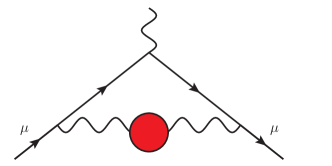
Figure 1: The leading, $\mathcal{O}(\alpha^{2})$, hadronic contribution to the muon $g$-2. The red blob indicates the HVP insertion.

2.2 Space-like method

The time-like expression for $a_{\mu}^{\rm HVP}({\rm LO})$ provided by Eq. (4) can be rewritten using the dispersion relation satisfied by $K^{(2)}(z)$ [40],

$$K^{(2)}(z)=\frac{1}{\pi}\int_{-\infty}^{0}\!{\rm d}z^{\prime}\,\frac{{\rm Im}K^{(2)}(z^{\prime})}{z^{\prime}-z},\quad z>0.$$ (8)

Indeed, replacing $K^{(2)}(s/m^{2})$ in Eq. (4) with Eq. (8) and integrating over $s$ via the subtracted dispersion relation satisfied by $\Pi_{\rm h}(q^{2})$,

$$\frac{\Pi_{\rm h}(q^{2})}{q^{2}}=\frac{1}{\pi}\int_{s_{0}}^{\infty}\frac{{\rm d}s}{s}\frac{{\rm Im}\Pi_{\rm h}(s)}{s-q^{2}},\quad q^{2}<0,$$ (9)

we obtain the space-like expression

$$a_{\mu}^{\rm HVP}({\rm LO})=-\frac{\alpha}{\pi^{2}}\int_{-\infty}^{0}\frac{{\rm d}t}{t}\,\Pi_{\rm h}(t)\,{\rm Im}K^{(2)}(t/m^{2}).$$ (10)

The function $K^{(2)}(z)$, real for any $z\geq 0$, has a cut along the negative real axis $z<0$ with the imaginary part

$${\rm Im}K^{(2)}(z+i\epsilon) =\pi\,\theta(-z)\!\left[\frac{z^{2}}{2}-z+\frac{z-2z^{2}+z^{3}/2}{\sqrt{z(z-4)}}\right]$$

$$=\pi\,\theta(-z)\,F^{(2)}(1/y(z)),$$ (11)

where

$$F^{(2)}(u)=\frac{u+1}{u-1}\,u^{2}.$$ (12)

The $i\epsilon$ prescription, with $\epsilon>0$, indicates that, in correspondence of the cut, the function Im$K^{(2)}(z)$ is evaluated approaching the real axis from above.

If in Eq. (10) one uses the explicit expression for ${\rm Im}K^{(2)}\!(t/m^{2})$ of Eq. (11) and changes the integration variable from $t$ to $x=1+1/y$ via the substitution

$$t(x)=\frac{m^{2}x^{2}}{x-1},$$ (13)

obtained from Eq. (6), one finds [41]

$$a_{\mu}^{\rm HVP}({\rm LO})=\frac{\alpha}{\pi}\int_{0}^{1}{\rm d}x\,\kappa^{(2)}(x)\,\Delta\alpha_{\rm h}(t(x)),$$ (14)

where the space-like kernel is remarkably simple,

$$\kappa^{(2)}(x)=1-x$$ (15)

and $\Delta\alpha_{\rm h}(t)=-\Pi_{\rm h}(t)$ is the (five-flavor) hadronic contribution to the running of the electromagnetic coupling in the space-like region, $\alpha(t)=\alpha/(1-\Delta\alpha(t))$.

Equation (14) (or forms equivalent to it) is used in lattice QCD calculations of $a_{\mu}^{\rm HVP}({\rm LO})$ (see e.g. [42] and a discussion in [7]) and forms the basis for the MUonE proposal to determine $a_{\mu}^{\rm HVP}({\rm LO})$ via muon-electron scattering data [33, 34, 35, 36].

We close this Section noting that, in Fig. 1, a virtual photon can be emitted and reabsorbed by the HVP insertion of the LO diagram. These irreducible hadronic contributions, although of higher order in $\alpha$, are normally incorporated into the time-like determination of $a_{\mu}^{\rm HVP}({\rm LO})$ via the inclusion of final-state radiation corrections in the $R$-ratio (see e.g. [7, 8]). For a comparison, also space-like evaluations of $a_{\mu}^{\rm HVP}({\rm LO})$ should therefore incorporate these higher-order corrections, including them in $\Delta\alpha_{\rm h}(t)$ in Eq. (14). In this respect, the fully inclusive measurement of $\Delta\alpha_{\rm h}(t)$ expected from MUonE is ideal [43].

3 The HVP contribution at NLO

The hadronic vacuum polarization contribution to the muon $g$-2 at NLO, $a_{\mu}^{\rm HVP}({\rm NLO})$ has been studied as early as in Ref. [44]. It is due to $\mathcal{O}(\alpha^{3})$ diagrams that can be classified as follows (see Fig. 2).

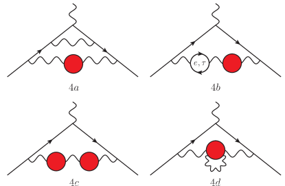
Figure 2: Sample $\mathcal{O}(\alpha^{3})$ diagrams contributing to the HVP corrections to the muon $g$-2.

Class $(4a)$ comprises diagrams with one single HVP insertion in one of the photon lines of the two-loop QED diagrams contributing to the muon $g$-2, without any VP insertion due to electron or tau loops. Class $(4b)$ contains diagrams with one HVP and one additional VP due to an electron or tau loop. Class $(4c)$ consists of the single diagram with two HVPs. Class $(4d)$ diagrams contain internal radiative corrections to the HVP. As discussed in the previous Section, this contribution is not considered as part of $a_{\mu}^{\rm HVP}({\rm NLO})$, although of the same order in $\alpha$, because it is already incorporated into $a_{\mu}^{\rm HVP}({\rm LO})$. Analogously, the $\mathcal{O}(\alpha^{4})$ contributions obtained by adding to the diagrams of classes $(4a)$, $(4b)$ and $(4c)$ a virtual photon emitted and reabsorbed by an HVP insertion, although of higher order in $\alpha$, should be incorporated into $a_{\mu}^{\rm HVP}({\rm NLO})$, either via the $R$-ratio (in the time-like approach) or via $\Delta\alpha_{\rm h}(t)$ (in the space-like one). If a second virtual photon is attached to the HVP insertion of class $(4d)$, the resulting contribution should be incorporated into $a_{\mu}^{\rm HVP}({\rm LO})$ (see also Section 4).

Numerically, class $(4a)$ yields the largest (negative) contribution, class $(4b)$ partially cancels it, and class $(4c)$ is small, as expected. Their sum

$$a_{\mu}^{\rm HVP}({\rm NLO})=a_{\mu}^{(4a)}+a_{\mu}^{(4b)}+a_{\mu}^{(4c)}$$ (16)

is negative and of $\mathcal{O}(10^{-9})$.

3.1 Class $(4a)$

The NLO HVP contribution of class $(4a)$ to the muon $g$-2 can be written in the time-like form [40]

$$a_{\mu}^{(4a)}=\frac{\alpha^{2}}{\pi^{3}}\int_{s_{0}}^{\infty}\frac{{\rm d}s}{s}\,2K^{(4)}(s/m^{2})\,{\rm Im}\Pi_{\rm h}(s).$$ (17)

The fourth-order function $K^{(4)}(z)$ was first computed by Barbieri and Remiddi in [40]. Its lengthy expression is reported in their Eq. (3.21) for $z>0$, where it is real and negative. An approximate series expansion for $K^{(4)}(s/m^{2})$ in the parameter $m^{2}/s$, with terms up to fourth order, can be found in [45].

Like $K^{(2)}(z)$, the function $K^{(4)}(z)$ is real for any $z\geq 0$, has a cut for $z<0$, and satisfies the dispersion relation

$$K^{(4)}(z)=\frac{1}{\pi}\int_{-\infty}^{0}\!{\rm d}z^{\prime}\,\frac{{\rm Im}K^{(4)}(z^{\prime})}{z^{\prime}-z},\quad z>0.$$ (18)

Just as we did for $a_{\mu}^{\rm HVP}({\rm LO})$, using the dispersion relations (9) and (18) the NLO hadronic contribution of class $(4a)$ can be cast in the space-like form

$$a_{\mu}^{(4a)}=-\frac{\alpha^{2}}{\pi^{3}}\int_{-\infty}^{0}\frac{{\rm d}t}{t}\,\Pi_{\rm h}(t)\,2{\rm Im}K^{(4)}(t/m^{2}).$$ (19)

The function ${\rm Im}K^{(4)}(t/m^{2})$ can be calculated from the $K^{(4)}(z)$ expression of Ref. [40]. Taking the imaginary parts of the polylogarithms of order 1, 2, and 3, we obtain

$${\rm Im}K^{(4)}(z+i\epsilon)=\pi\,\theta(-z)\,F^{(4)}(1/y(z)),$$ (20)

where

$$F^{(4)}(u) =R_{1}(u)+R_{2}(u)\ln(-u)$$

$$\,+R_{3}(u)\ln(1+u)+R_{4}(u)\ln(1-u)$$

$$\,+R_{5}(u)\big{[}4{\rm Li}_{2}(u)+2{\rm Li}_{2}(-u)$$

$$~{}~{}~{}~{}+\ln(-u)\ln\!\left((1-u)^{2}(1+u)\right)\!\big{]},$$ (21)

and the rational functions $R_{i}(u)$ $(i=1,\ldots,5)$ are

$$R_{1}\!= \frac{23u^{6}\!-\!37u^{5}\!+\!124u^{4}\!-\!86u^{3}\!-\!57u^{2}\!+\!99u\!+\!78}{72(u-1)^{2}u(u+1)},$$

$$R_{2}\!= \frac{12u^{8}\!-\!11u^{7}\!-\!78u^{6}\!+\!21u^{5}\!+\!4u^{4}\!-\!15u^{3}\!+\!13u\!+\!6}{12(u-1)^{3}u(u+1)^{2}},$$

$$R_{3}\!= \frac{(u+1)\left(-u^{3}+7u^{2}+8u+6\right)}{12u^{2}},$$

$$R_{4}\!= \frac{-7u^{4}-8u^{3}+8u+7}{12u^{2}},$$

$$R_{5}\!= -\frac{3u^{4}+5u^{3}+7u^{2}+5u+3}{6u^{2}}.$$ (22)

The dilogarithm is ${\rm Li}_{2}(u)=-\int_{0}^{u}({\rm d}v/v)\ln(1-v)$.

Using the explicit expression for ${\rm Im}K^{(4)}\!(t/m^{2})$ of Eq. (20), Eq. (19) can be conveniently expressed in terms of the variable $x=1+1/y$. We obtain

$$a_{\mu}^{(4a)}=\left(\frac{\alpha}{\pi}\right)^{2}\!\int_{0}^{1}{\rm d}x\,\kappa^{(4)}(x)\,\Delta\alpha_{\rm h}(t(x)),$$ (23)

where

$$\kappa^{(4)}(x)=\frac{2-x}{x\left(x-1\right)}\,2F^{(4)}(x-1).$$ (24)

For $0\leq x<1$, $z\leq 0$. Equation (23) is the analogue of Eq. (14) for the NLO contribution of class $(4a)$.

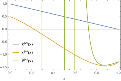
Figure 3: The space-like functions $\kappa^{(2)}(x)$ (blue), $\kappa^{(4)}(x)$ (orange) and $\tilde{\kappa}^{(4)}(x)$ (green).

Figure 3 shows the space-like functions $\kappa^{(2)}(x)$ and $\kappa^{(4)}(x)$ entering the $a_{\mu}^{\rm HVP}({\rm LO})$ and $a_{\mu}^{(4a)}$ expressions, respectively. We note that the function $\kappa^{(4)}(x)$ provides a stronger weight to $\Delta\alpha_{\rm h}(q^{2})$ at large negative values of $q^{2}$ than $\kappa^{(2)}(x)$. In particular, for $q^{2}\to-\infty$, $\kappa^{(2)}(1)=0$, whereas $\kappa^{(4)}(1)=-23/18$. Figure 4 shows the LO integrand $(\alpha/\pi)\kappa^{(2)}(x)\Delta\alpha_{\rm h}(t(x))$ of Eq. (14) and the NLO integrand $(\alpha/\pi)^{2}\kappa^{(4)}(x)\Delta\alpha_{\rm h}(t(x))$ of Eq. (23), multiplied by $10^{7}$ and $-10^{8}$, respectively. The LO integrand has a peak at $x\sim 0.914$, where $t\sim-(0.33{\rm GeV})^{2}$. On the other hand, the NLO integrand of class $(4a)$ increases monotonically with $x\to 1$ (i.e. with $t\to-\infty$) like $\sim\ln(1-x)$.

An approximate expression for the space-like formula in Eq. (23) was provided in Ref. [26]. To obtain it, the authors started considering the approximate fourth-order series expansion of Ref. [45] for the time-like function $K^{(4)}(s/m^{2})$ in the small parameter $r=m^{2}/s$. This series expansion contains only powers $r^{n}$ of degree $n=1,2,3,4$, multiplied by constants, $\ln r$, and $(\ln r)^{2}$ terms. Then, as suggested in [49], they exploited generating integral representations to fit the $r^{n}$ and $r^{n}\!\ln r$ terms of the approximate fourth-order series expansion for $K^{(4)}(1/r)$, but not the $r^{n}(\ln r)^{2}$ ones, and used the usual dispersion relation satisfied by $\Pi_{\rm h}(q^{2})$ to perform the integral over $s$. After simple changes of variables, their approximation can be compared with our exact function $\kappa^{(4)}(x)$. We repeated the analysis of Ref. [26] confirming their approximate result (in particular, their Eqs. (A1,A2)) which, translated in our notation, is called here $\tilde{\kappa}^{(4)}(x)$.

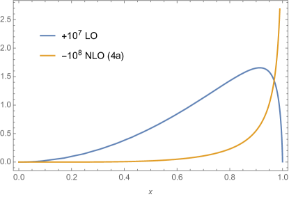
Figure 4: The integrands $(\alpha/\pi)\kappa^{(2)}(x)\Delta\alpha_{\rm h}(t(x))$ (blue) and $(\alpha/\pi)^{2}\kappa^{(4)}(x)\Delta\alpha_{\rm h}(t(x))$ (orange) of Eqs.(14) and (23), multiplied by $10^{7}$ and $-10^{8}$, respectively.

The approximate function $\tilde{\kappa}^{(4)}(x)$ is plotted in Fig. 3 (indicated by the green line). While the exact function $\kappa^{(4)}(x)$ varies smoothly over the entire region $0\leq x\leq 1$, $\tilde{\kappa}^{(4)}(x)$ strongly oscillates, leading to large numerical cancelations when employed in the integral of Eq. (23) instead of $\kappa^{(4)}(x)$. Using the Fortran libraries KNT18VP [50, 51, 52, 53, 54, 10] for the numerical implementation of $\Delta\alpha_{\rm h}(t(x))$ in the space-like region, we computed two numerical values for $a_{\mu}^{(4a)}$ in Eq. (23): one obtained using the exact function $\kappa^{(4)}(x)$ and a second one obtained replacing $\kappa^{(4)}(x)$ with the approximate $\tilde{\kappa}^{(4)}(x)$. The two values differ by about 3%. Adding to $a_{\mu}^{(4a)}$ the contributions $a_{\mu}^{(4b)}$ and $a_{\mu}^{(4c)}$ (discussed later), the total $a_{\mu}^{\rm HVP}({\rm NLO})$ contribution computed using the $\tilde{\kappa}^{(4)}(x)$ approximation differs from the one computed via our exact function $\kappa^{(4)}(x)$ by about 6%.

It is interesting to investigate the source of the above $\sim 6$% discrepancy. To improve the $\tilde{\kappa}^{(4)}(x)$ approximation, we proceeded in two directions. The first one consisted in repeating the analysis of Ref. [26], starting however from higher-order series expansions for the exact $K^{(4)}(s/m^{2})$ function of Barbieri and Remiddi [40] (we considered $n$ up to $n_{\rm max}=24$), rather than from the fourth-order (i.e. $n_{\rm max}=4$) series expansion for $K^{(4)}(s/m^{2})$ of Ref. [45]. Our second improvement consisted in exploiting generating integral representations to fit the $r^{n}$, $r^{n}\!\ln r$, as well as the $r^{n}(\ln r)^{2}$ terms which were omitted in the analysis of Ref. [26]. Our studies show that the inclusion of the $r^{n}(\ln r)^{2}$ terms greatly improves the $\kappa^{(4)}(x)$ approximations, even if the order $n_{\rm max}$ of the series expansion for $K^{(4)}(s/m^{2})$ is not increased above four. Calling $\bar{\kappa}^{(4)}(x,n_{\rm max})$ our improved approximations to $\kappa^{(4)}(x)$, obtained including $r^{n}(\ln r)^{2}$ terms and starting from series expansions for $K^{(4)}(s/m^{2})$ up to order $n_{\rm max}$, we verified that the total $a_{\mu}^{\rm HVP}({\rm NLO})$ contribution computed using our $\bar{\kappa}^{(4)}(x,4)$ differs by less than one per mille from the one computed via our exact function $\kappa^{(4)}(x)$. Even better agreements were reached increasing the order $n_{\rm max}$.

The authors of Ref. [26] added an $O(10\%)$ uncertainty to their final result to take into account the error induced by the omission of the $r^{n}(\ln r)^{2}$ terms. This uncertainty, which dominates the error of their final result, can be eliminated using the exact formula for $\kappa^{(4)}(x)$ provided in this paper.

3.2 Classes $(4b)$ and $(4c)$

The space-like expressions for the contributions of classes $(4b)$ and $(4c)$ to the muon $g$-2 are [8, 26]

$$a_{\mu}^{(4b)} =\frac{\alpha}{\pi}\int_{0}^{1}{\rm d}x\,\kappa^{(2)}(x)\,\Delta\alpha_{\rm h}(t(x))$$

$$~{}~{}~{}~{}~{}~{}~{}\times 2\left[\Delta\alpha_{e}^{(2)}(t(x))+\Delta\alpha_{\rm\tau}^{(2)}(t(x))\right],$$ (25)

$$a_{\mu}^{(4c)} =\frac{\alpha}{\pi}\int_{0}^{1}{\rm d}x\,\kappa^{(2)}(x)\,\left[\Delta\alpha_{\rm h}(t(x))\right]^{2},$$ (26)

where $\Pi_{\ell}^{(2)}(t)=-\Delta\alpha_{\ell}^{(2)}(t)$ is the renormalized one-loop QED VP function in the space-like region, with a lepton $\ell=e,\tau$ of mass $m_{\ell}$ in the loop,

$$\Pi_{\ell}^{(2)}(t)=\frac{\alpha}{\pi}\left[\frac{8}{9}-\frac{\beta_{\ell}^{2}}{3}+\beta_{\ell}\!\left(\frac{1}{2}-\frac{\beta^{2}_{\ell}}{6}\right)\!\ln\frac{\beta_{\ell}-1}{\beta_{\ell}+1}\right]$$ (27)

and $\beta_{\ell}=\sqrt{1-4m_{\ell}^{2}/t}$. Equations (3.2,26) can be immediately obtained from the time-like formulae of Ref. [45] using the usual dispersion relation satisfied by $\Pi_{\rm h}(t)$ and $\Pi_{\ell}^{(2)}(t)$ to perform the integrals over $s$ [41, 26].

Figure 5 shows the NLO integrands of Eqs. (23), (3.2), and (26), multiplied by $-10^{8}$, $10^{8}$, and $10^{8}$, respectively.

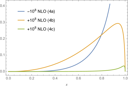
Figure 5: The NLO integrands of Eqs. (23) (blue), (3.2) (orange), and (26) (green), multiplied by $-10^{8}$, $10^{8}$, and $10^{8}$, respectively.

4 The HVP contribution at NNLO

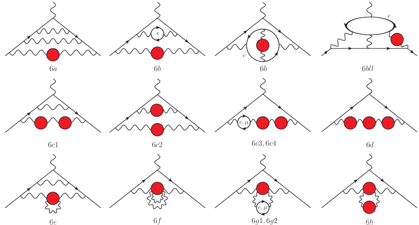
Figure 6: Sample $\mathcal{O}(\alpha^{4})$ diagrams contributing to the HVP corrections to the muon $g$-2.

The hadronic vacuum polarization contribution to the muon $g$-2 at NNLO, $a_{\mu}^{\rm HVP}({\rm NNLO})$, is due to several diagrams of $\mathcal{O}(\alpha^{4})$. We divide them into the following classes (see Fig. 6). Class $(6a)$ contains diagrams with one HVP insertion and up to two photons added to the LO QED Feynman graph; it also includes diagrams with one or two muon VP loops and the light-by-light graph with a muon loop. Class $(6b)$ comprises diagrams with one HVP insertion and one or two electron VP loops and additional photonic or muon VP corrections; it also includes diagrams with one electron VP loop with an HVP insertion inside it. Class $(6bll)$ diagrams have one HVP insertion and light-by-light graphs with an electron loop; in these diagrams, the external photon couples to the electron. Class $(6c)$ contains diagrams with two HVP insertions and additional photonic corrections and/or electron or muon VP loops. Class $(6d)$ consists of the diagram with three HVP insertions. All of these classes were studied in Ref. [16] in the time-like approach.

Class $(6e)$ diagrams are obtained by adding to those of classes $(4a)$, $(4b)$ and $(4c)$ a virtual photon emitted and reabsorbed by an HVP insertion. As discussed in the previous Section, their contribution should not be considered as part of $a_{\mu}^{\rm HVP}({\rm NNLO})$, although of the same order in $\alpha$, because it is already incorporated into $a_{\mu}^{\rm HVP}({\rm NLO})$ via the $R$-ratio (in the time-like approach) or via $\Delta\alpha_{\rm h}(t)$ (in the space-like one). Similarly, the corrections of class $(6f)$, where two photons are emitted and reabsorbed by the HVP insertion of the LO diagram, should be already included in $a_{\mu}^{\rm HVP}({\rm LO})$. The impact of class $(6f)$ can be roughly estimated considering the corresponding class of diagrams where the HVP insertion is replaced by a muon VP; that four-loop QED contribution to the muon $g$-2 is $1.44\times 10^{-12}$ [56]. The effect of class $(6f)$ can thus be roughly estimated to be of $\mathcal{O}(10^{-12})$. The contribution of class $(6g1)$ was recently studied in Ref. [55], where it was estimated to be $\lesssim 1\times 10^{-11}$. The impact of classes $(6g2)$ and $(6h)$ can be roughly estimated, once again, considering the corresponding four-loop QED contribution to the muon $g$-2 where the HVP insertions are replaced by muon VPs: $3.24\times 10^{-13}$ [56]. The effect of classes $(6g2)$ and $(6h)$ can thus be roughly estimated to be of $\mathcal{O}(10^{-13})$. Classes $(6f)$, $(6g1)$, $(6g2)$ and $(6h)$ should be incorporated into $a_{\mu}^{\rm HVP}({\rm LO})$.

The sum of the NNLO contributions is, therefore,

$$a_{\mu}^{\rm HVP}({\rm NNLO})=a_{\mu}^{(6a)}+a_{\mu}^{(6b)}+a_{\mu}^{(6bll)}+a_{\mu}^{(6c)}+a_{\mu}^{(6d)}.$$ (28)

It is positive and of $\mathcal{O}(10^{-10})$ [16].

4.1 Class $(6a)$

The contribution of class $(6a)$ can be written in the time-like form [16]

$$a_{\mu}^{(6a)}=\frac{\alpha^{3}}{\pi^{4}}\int_{s_{0}}^{\infty}\frac{{\rm d}s}{s}\,K^{(6a)}(s/m^{2})\,{\rm Im}\Pi_{\rm h}(s).$$ (29)

The sixth-order function $K^{(6a)}(z)$ is not known in exact form, but an approximate series expansion in the parameter $r=m^{2}/s$, with terms up to fourth order, was computed in [16]. This expansion contains powers $r^{n}$ of degree $n=1,2,3,4$, multiplied by constants, $\ln r$, $(\ln r)^{2}$ and $(\ln r)^{3}$ terms. Following a procedure similar to that described at NLO, we exploited generating integral representations to fit all the $r^{n}$, $r^{n}\!\ln r$, $r^{n}(\ln r)^{2}$, and $r^{n}(\ln r)^{3}$ terms of the $K^{(6a)}(s/m^{2})$ expansion,

$$K^{(6a)}(s/m^{2})=r\!\int_{0}^{1}\!\!{\rm d}\xi\!\left[\frac{L^{(6a)}(\xi)}{\xi+r}+\frac{P^{(6a)}(\xi)}{1+r\xi}\right]$$ (30)

where

$$L^{(6a)}(\xi)=G^{(6a)}(\xi)+H^{(6a)}(\xi)\ln\xi+J^{(6a)}(\xi)\ln^{2}\!\xi$$ (31)

and

$$G^{(6a)}(\xi) =g_{0}^{(6a)}\!+g_{1}^{(6a)}\xi+g_{2}^{(6a)}\xi^{2}\!+g_{3}^{(6a)}\xi^{3},$$

$$H^{(6a)}(\xi) =h_{0}^{(6a)}\!+h_{1}^{(6a)}\xi+h_{2}^{(6a)}\xi^{2}\!+h_{3}^{(6a)}\xi^{3},$$

$$J^{(6a)}(\xi) =j_{0}^{(6a)}\!+j_{1}^{(6a)}\xi+j_{2}^{(6a)}\xi^{2}\!+j_{3}^{(6a)}\xi^{3},$$

$$P^{(6a)}(\xi) =p_{0}^{(6a)}\!+p_{1}^{(6a)}\xi+p_{2}^{(6a)}\xi^{2}\!+p_{3}^{(6a)}\xi^{3},$$ (32)

obtaining the coefficients $g_{i}^{(6a)}$, $h_{i}^{(6a)}$, $j_{i}^{(6a)}$ and $p_{i}^{(6a)}$ ($i=0,1,2,3$) reported in Table 1.

Inserting the integral representation of Eq. (30) in Eq. (29), the integral over $s$ can be performed using the dispersion relation satisfied by $\Pi_{\rm h}(q^{2})$. With simple changes of variables we obtain

$$a_{\mu}^{(6a)}=\left(\frac{\alpha}{\pi}\right)^{3}\!\int_{0}^{1}{\rm d}x\,\bar{\kappa}^{(6a)}(x)\,\Delta\alpha_{\rm h}(t(x)),$$ (33)

where, for $0<x<x_{\mu}=(\sqrt{5}-1)/2=0.618\ldots$,

$$\bar{\kappa}^{(6a)}(x)\,=\,\frac{2-x}{x\left(1-x\right)}\,P^{(6a)}\!\!\left(\frac{x^{2}}{1-x}\right),$$ (34)

whereas, for $x_{\mu}<x<1$,

$$\bar{\kappa}^{(6a)}(x)\,=\,\frac{2-x}{x^{3}}\,L^{(6a)}\!\!\left(\frac{1-x}{x^{2}}\right).$$ (35)

We note that for $x=x_{\mu}$, $t=-m^{2}$. The uncertainty of Eq. (33) due to the series approximation of $K^{(6a)}$ is estimated to be less than $O(10^{-12})$.

4.2 Classes $(6b)$ and $(6bll)$

The contributions of classes $(6b)$ and $(6bll)$ can be calculated similarly to class $(6a)$. Indeed, in the time-like region, $a_{\mu}^{(6b)}$ and $a_{\mu}^{(6bll)}$ can be computed via Eq. (29) replacing $K^{(6a)}$ with $K^{(6b)}$ and $K^{(6bll)}$, respectively. For these sixth-order kernel functions, approximate series expansions in the parameters $r=m^{2}/s$ and $\rho=m_{e}/m$ were computed in [16]. The highest order expansion terms provided are of $O(\rho^{2}r^{4})$. Following the same procedure described in Subsection 4.1, we fit these expansions obtaining integral representations analogous to that of Eq. (30) with the coefficients $g_{i}^{(6b)}$, $h_{i}^{(6b)}$, $j_{i}^{(6b)}$, $p_{i}^{(6b)}$ and $g_{i}^{(6bll)}$, $h_{i}^{(6bll)}$, $j_{i}^{(6bll)}$, $p_{i}^{(6bll)}$ reported in Table 2 and 3, respectively. The contributions $a_{\mu}^{(6b)}$ and $a_{\mu}^{(6bll)}$ can then be calculated in the space-like region using Eqs. (33–35), mutatis mutandis. Their estimated uncertainties due to the series approximations are less than $O(10^{-12})$.

4.3 Class $(6c)$

The contribution of class $(6c)$ in the time-like region is given by [16]

$$a_{\mu}^{(6c)}=\,\, \frac{\alpha^{2}}{\pi^{4}}\int_{s_{0}}^{\infty}\frac{{\rm d}s}{s}\frac{{\rm d}s^{\prime}}{s^{\prime}}\,K^{(6c)}(s/m^{2},s^{\prime}/m^{2})\,\times$$

$$\times{\rm Im}\Pi_{\rm h}(s)\,{\rm Im}\Pi_{\rm h}(s^{\prime}).$$ (36)

As class $(6c)$ diagrams contain two HVP insertions, the time-like formula (36) for $a_{\mu}^{(6c)}$ requires two dispersive integrations of ${\rm Im}\Pi_{\rm h}(s)$. Asymptotic expansions were provided in Ref. [16] for the function $K^{(6c)}(s/m^{2},s^{\prime}/m^{2})$ in the limits $s^{\prime}\approx s\gg m^{2}$ and $s^{\prime}\gg s\gg m^{2}$, from which an approximation of $K^{(6c)}(s/m^{2},s^{\prime}/m^{2})$ valid for all values of $s^{\prime}$ and $s$ much larger than $m^{2}$ can be constructed.

In the time-like approach, the number of dispersive integrations of ${\rm Im}\Pi_{\rm h}(s)$ required to calculate the contribution of a diagram to the muon $g$-2 is given by the number of HVP insertions. On the other hand, the required dimension of the space-like integral of $\Delta\alpha_{\rm h}(t)$ (or powers of it) equals the number of photon lines with different momenta containing HVP insertions. To obtain a space-like formula for $a_{\mu}^{(6c)}$, it is therefore convenient to separate the diagrams of class $(6c)$ into the following four subclasses $(6c1)$, $(6c2)$, $(6c3)$, and $(6c4)$ (see Fig. 6).

The diagrams of subclass $(6c1)$ contain two HVP insertions in the same photon line and no other electron or muon loop. The exact space-like expression for their contribution to the muon $g$-2 is therefore given by the one-dimensional integral

$$a_{\mu}^{(6c1)}=\left(\frac{\alpha}{\pi}\right)^{2}\!\int_{0}^{1}{\rm d}x\,\lambda^{(4)}(x)\,\left[\Delta\alpha_{\rm h}(t(x))\right]^{2},$$ (37)

where the kernel function is

$$\lambda^{(4)}(x)\,=\,\kappa^{(4)}(x)\,-\,\frac{2\pi}{\alpha}\kappa^{(2)}(x)\,\Delta\alpha_{\mu}^{(2)}(t(x)),$$ (38)

$\kappa^{(4)}(x)$ is the exact fourth-order space-like kernel of Eq. (24) and $\kappa^{(2)}(x)$ is the lowest-order one of Eq. (15). In Eq. (37), the use of the subtracted kernel $\lambda^{(4)}(x)$ instead of $\kappa^{(4)}(x)$ guarantees the subtraction of the contribution, induced by $\kappa^{(4)}(x)$, of two diagrams containing two HVP and one muon VP in the same photon line.

The contribution of the three diagrams of subclass $(6c3)$, containing two HVP and one electron VP insertion in the same photon line, can be cast in the exact space-like one-dimensional integral form

$$a_{\mu}^{(6c3)}=\frac{3\alpha}{\pi}\int_{0}^{1}{\rm d}x\,\kappa^{(2)}(x)\left[\Delta\alpha_{\rm h}(t(x))\right]^{2}\!\Delta\alpha_{e}^{(2)}(t(x)).$$ (39)

Analogously, the exact contribution of subclass $(6c4)$, comprising three diagrams with two HVP and one muon VP insertion in the same photon line, can be simply obtained replacing $\Delta\alpha_{e}^{(2)}(t)$ with $\Delta\alpha_{\mu}^{(2)}(t)$ in Eq. (39).

Subclass $(6c2)$ consists of diagrams with two HVP insertions in two different photon lines. Contrary to the simple one-dimensional integral form of all the space-like expressions for the contributions to the muon $g$-2 discussed so far, the presence in $(6c2)$ of two different photon lines with HVP insertions requires a double space-like integration. We therefore proceeded in two steps. First, we computed the approximate time-like kernel $K^{(6c2)}(s/m^{2},s^{\prime}/m^{2})$ for the subclass $(6c2)$. This was obtained by calculating the exact time-like kernels $K^{(6c1)}(s/m^{2},s^{\prime}/m^{2})$, $K^{(6c3)}(s/m^{2},s^{\prime}/m^{2})$ and $K^{(6c4)}(s/m^{2},s^{\prime}/m^{2})$ from the exact space-like expressions of Eqs.(37,39), computing the series expansion of these kernels in the limits $s^{\prime}\approx s\gg m^{2}$ and $s^{\prime}\gg s\gg m^{2}$, and finally subtracting the obtained results from the $K^{(6c)}(s/m^{2},s^{\prime}/m^{2})$ approximation of Ref. [16]. As a second step, we matched the LO terms of the approximate time-like kernel $K^{(6c2)}(s/m^{2},s^{\prime}/m^{2})$ with those of the series expansion of a two-dimensional generating integral representation, generalising to two-dimensions the method used earlier to fit the $K^{(6a)}(s/m^{2})$ expansion. Our result for the space-like expression of the contribution of subclass $(6c2)$ to the muon $g$-2 is

$$a_{\mu}^{(6c2)}\,=\, \left(\frac{\alpha}{\pi}\right)^{2}\!\int_{x_{\mu}}^{1}\!{\rm d}x\int_{x_{\mu}}^{1}\!{\rm d}x^{\prime}\,\bar{\kappa}^{(6c2)}(x,x^{\prime})\,\times$$

$$\times\Delta\alpha_{\rm h}(t(x))\Delta\alpha_{\rm h}(t(x^{\prime})),$$ (40)

where, for $x_{\mu}<\{x,x^{\prime}\}<1$,

$$\bar{\kappa}^{(6c2)}(x,x^{\prime})\,=\,\frac{2-x}{x^{3}}\frac{2-x^{\prime}}{x^{\prime 3}}\,G^{(6c2)}\!\!\left(\frac{1-x}{x^{2}},\frac{1-x^{\prime}}{x^{\prime 2}}\right)$$ (41)

and

$$\!\!G^{(6c2)}(\xi,\xi^{\prime})\,=\,\,\frac{1}{4\left(32\pi^{2}-315\right)}\, \times$$

$$\times\biggl{[}\left(1855-188\pi^{2}\right) \,\frac{\min(\xi,\xi^{\prime})}{\max(\xi,\xi^{\prime})^{2}}\,+$$

$$+\left(988\pi^{2}-9765\right) \,\frac{\min(\xi,\xi^{\prime})^{2}}{\max(\xi,\xi^{\prime})^{3}}\,+$$

$$+24\left(435-44\pi^{2}\right) \,\frac{\min(\xi,\xi^{\prime})^{3}}{\max(\xi,\xi^{\prime})^{4}}\biggr{]}.$$ (42)

This contribution is of $O(10^{-12})$. We note that the limits of integration in Eq. (40) are $x_{\mu}$ and 1, corresponding to values of $t$ between $-m^{2}$ and $-\infty$, respectively.

Equation (40) completes the list of space-like expressions for the contributions of class $(6c)$,

$$a_{\mu}^{(6c)}=a_{\mu}^{(6c1)}+a_{\mu}^{(6c2)}+a_{\mu}^{(6c3)}+a_{\mu}^{(6c4)}.$$ (43)

The uncertainty of Eq. (43) due to the approximations of subclass $(6c2)$ is less than $O(10^{-12})$.

4.4 Class $(6d)$

The correction due to the single diagram of class $(6d)$ can be written in the time-like form [16]

$$a_{\mu}^{(6d)}\,=\,\, \frac{\alpha}{\pi^{4}}\int_{s_{0}}^{\infty}\frac{{\rm d}s}{s}\frac{{\rm d}s^{\prime}}{s^{\prime}}\frac{{\rm d}s^{\prime\prime}}{s^{\prime\prime}}\,K^{(6d)}(s,s^{\prime},s^{\prime\prime})\,\times$$

$$\times{\rm Im}\Pi_{\rm h}(s)\,{\rm Im}\Pi_{\rm h}(s^{\prime})\,{\rm Im}\Pi_{\rm h}(s^{\prime\prime}).$$ (44)

The kernel $K^{(6d)}(s,s^{\prime},s^{\prime\prime})$ for the triple hadronic insertion is provided in [16] in integral form. On the other hand, the space-like expression for $a_{\mu}^{(6d)}$ can be cast in the simple exact form [8]

$$a_{\mu}^{(6d)}\,=\,\frac{\alpha}{\pi}\int_{0}^{1}{\rm d}x\,\kappa^{(2)}(x)\,\left[\Delta\alpha_{\rm h}(t(x))\right]^{3}.$$ (45)

We note that three dispersive integrations of ${\rm Im}\Pi_{\rm h}(s)$ are required to compute $a_{\mu}^{(6d)}$ in the time-like approach, whereas the space-like Eq. (45) involves only a one-dimensional integral. Numerically, $a_{\mu}^{(6d)}$ is very small, of $O(10^{-13})$.

5 Conclusions

This paper provides simple analytic expressions to calculate the HVP contributions to the muon $g$-2 in the space-like region up to NNLO. These results can be employed in lattice QCD computations of $a_{\mu}^{\rm HVP}$ as well as in determinations based on scattering data, like those expected from the proposed MUonE experiment at CERN.

After a derivation of the space-like formula for the HVP contribution at LO, obtained using the dispersion relation satisfied by the LO time-like kernel $K^{(2)}(z)$, we presented simple exact analytic expressions to extend the space-like calculation of $a_{\mu}^{\rm HVP}$ to NLO. The shapes of the space-like integrands of the $a_{\mu}^{\rm HVP}({\rm NLO})$ contributions were found to differ significantly from the LO one. In particular, the exact NLO space-like kernel $\kappa^{(4)}(x)$ provides a stronger weight to $\Delta\alpha_{\rm h}(q^{2})$ at large negative values of $q^{2}$ than the LO kernel $\kappa^{(2)}(x)$. These different weights may help to shed light on the present tension between the lattice QCD determination of $a_{\mu}^{\rm HVP}({\rm LO})$ by the BMW collaboration and the time-like data-driven ones.

The approximation to the NLO space-like kernel $\kappa^{(4)}(x)$ obtained by the authors of Ref. [26] induced the largest source of uncertainty of their NLO lattice QCD calculation of $a_{\mu}^{\rm HVP}({\rm NLO})$. This uncertainty, of $O(10\%)$, can be eliminated using the exact expression for $\kappa^{(4)}(x)$ provided in this paper.

The NNLO HVP contribution to the muon $g$-2 is comparable to the final uncertainty expected from the Muon $g$-2 experiment at Fermilab. We presented simple analytic space-like expressions for all the classes of diagrams representing these corrections. For the diagrams composed of one- or two-loop QED vertices and two or more HVP insertions in the same photon line, we obtained exact space-like integral formulas. For the diagrams containing actual three-loop QED vertices, like e.g. electron or muon light-by-light graphs, exploiting generating integral representations to fit the large-$s$ approximate series expansions of the time-like kernels provided by Ref. [16], we found very good approximations to the space-like kernels. The uncertainty of $a_{\mu}^{\rm HVP}({\rm NNLO})$ due to these kernel approximations is estimated to be less than $O(10^{-12})$.

In the space-like approach, the minimum dimension of the space-like integral of $\Delta\alpha_{\rm h}(t)$ (or powers of it) required to calculate the contribution of a diagram to the muon $g$-2 is given by the number of photon lines with different momenta containing HVP insertions. The space-like kernels to compute $a_{\mu}^{\rm HVP}$ at LO and NLO are therefore one-dimensional. The same is true at NNLO, with the notable exception of the class of diagrams with two HVP insertions in two different photon lines. For this class, a two-dimensional kernel is required. Generalising to two dimensions the one-dimensional method used earlier, we derived a good approximate two-dimensional space-like kernel matching the approximate time-like kernel with the series expansion of a two-dimensional generating integral representation. Once again, the uncertainty due to the kernel approximation is less than $O(10^{-12})$.

The calculation of higher-order HVP corrections to the muon $g$-2 requires a precise treatment of the QED radiative corrections to the HVP function. Their leading effect, induced by the emission and reabsorption of a photon by the HVP insertion, is normally incorporated into the time-like approach via the inclusion of final-state radiation corrections in the $R$-ratio. This is a notoriously delicate issue, because of the experimental cuts imposed by the analyses. On the other hand, the fully inclusive measurement of $\Delta\alpha_{\rm h}(t)$ expected from MUonE will naturally include these leading corrections in the space-like approach.

In conclusion, the results presented in this paper allow to compare, for the first time, time-like and space-like calculations of $a_{\mu}^{\rm HVP}$ at NNLO accuracy. These eagerly anticipated comparisons will strengthen the SM prediction of the muon $g$-2 enhancing its potential to unveil new physics.

Acknowledgments We would like to thank V. Barigelli, G. Colangelo, M. Fael, M. Hoferichter, A. Keshavarzi, W. J. Marciano, M. Steinhauser and G. Venanzoni for useful discussions and correspondence. We are also grateful to all our MUonE colleagues for our stimulating collaboration. M. P. acknowledges partial support from the EU Horizon 2020 research and innovation programme under the Marie Sklodowska-Curie grant agreements 101006726 (aMUSE) and 789410 (HIDDeN).

$(6a)$
$j_{0}=0$; $j_{1}=-\frac{3793}{864}$; $j_{2}=\frac{35087}{21600}$; $j_{3}=\frac{1592093}{43200}$;	$h_{0}=-\frac{359}{36}$; $h_{1}=\frac{122293}{5184}$; $h_{2}=-\frac{43879427}{648000}$; $h_{3}=\frac{14388407}{48000}$;
$g_{0}=\frac{1301}{144}-\frac{19\pi^{2}}{9}$; $g_{1}=\frac{441277}{10368}+\pi^{2}\left(-\frac{355}{648}+\ln{4}\right)+\frac{25\ \zeta(3)}{2}$; $g_{2}=-\frac{5051645167}{38880000}+\pi^{2}\left(\frac{221411}{32400}-18\ln{2}\right)-\frac{3919\ \zeta(3)}{60}$; $g_{3}=\frac{14588342017}{38880000}+\pi^{2}\left(-\frac{2479681}{64800}+112\ln{2}\right)+\frac{3113\ \zeta(3)}{10}$;
$p_{0}=-\frac{1808080780513}{14580000}+\frac{41851\pi^{4}}{15}+\frac{8432\ln^{4}{2}}{3}+67456\ a_{4}+\frac{2085448\ \zeta(3)}{15}+$       $+\pi^{2}\left(-\frac{11944163099}{194400}+\frac{272}{3}\left(180-31\ln{2}\right)\ln{2}+\frac{115072\ \zeta(3)}{3}\right)-\frac{575360\ \zeta(5)}{3}$; $p_{1}=\frac{134017456919}{96000}-\frac{4481182\pi^{4}}{135}-\frac{98420\ln^{4}{2}}{3}-787360\ a_{4}+2255200\ \zeta(5)+$       $+\pi^{2}\left(\frac{23549054249}{32400}-201122\ln{2}+\frac{98420\ln^{2}{2}}{3}-451040\ \zeta(3)\right)-\frac{57189259\ \zeta(3)}{36}$; $p_{2}=-\frac{13069081405453}{3888000}+\frac{330073\pi^{4}}{4}+80790\ln^{4}{2}+1938960\ a_{4}+\frac{77371609\ \zeta(3)}{20}+$       $+\pi^{2}\left(-\frac{729995599}{405}+6\left(85313-13465\ln{2}\right)\ln{2}+1114360\ \zeta(3)\right)-5571800\ \zeta(5)$; $p_{3}=\frac{1274611832039}{583200}-\frac{986377\pi^{4}}{18}-53340\ln^{4}{2}-1280160\ a_{4}+\frac{11057200\ \zeta(5)}{3}+$       $+\pi^{2}\left(\frac{5809659289}{4860}+420\ln{2}\left(-823+127\ln{2}\right)-\frac{2211440\ \zeta(3)}{3}\right)-\frac{22833188\ \zeta(3)}{9}$;

Table 1: The coefficients $g_{i}^{(6a)}$, $h_{i}^{(6a)}$, $j_{i}^{(6a)}$, $p_{i}^{(6a)}$ ($i=0,1,2,3$). The superscript ${(6a)}$ has been dropped for simplicity. In the above coefficients, the Riemann zeta function $\zeta(k)=\sum_{n=1}^{\infty}1/n^{k}$ and $a_{4}=\sum_{n=1}^{\infty}1/(2^{n}n^{4})={\rm Li}_{4}(1/2)$.

$(6b)$
$j_{0}=0$; $j_{1}=\frac{11}{27}$; $j_{2}=\frac{41}{120}$; $j_{3}=-\frac{507}{40}$;	$h_{0}=\frac{65}{54}$; $h_{1}=-\frac{3559}{1296}+\rho^{2}+\frac{5}{18}\ln{\rho}$; $h_{2}=\frac{3917}{432}-\frac{82\rho^{2}}{3}+\frac{61}{10}\ln{\rho}$; $h_{3}=-\frac{4109}{80}+\frac{2211\rho^{2}}{10}-\frac{1763}{30}\ln{\rho}$;
$g_{0}=\frac{1}{108}\left(259-72\rho^{2}+276\ln{\rho}\right)$; $g_{1}=-\frac{9215}{1296}+\frac{65\pi^{2}}{162}-\frac{3\pi^{2}\rho}{4}+\frac{49\rho^{2}}{36}+\left(-\frac{301}{54}+8\rho^{2}\right)\ln{\rho}+\frac{4}{3}\ln^{2}{\rho}+2\ \zeta(3)$; $g_{2}=\frac{501971}{40500}-\frac{113\pi^{2}}{36}+\frac{270\pi^{2}\rho}{36}-\frac{8417\rho^{2}}{180}+\left(\frac{3479}{900}-44\rho^{2}\right)\ln{\rho}-8\ln^{2}{\rho}-12\ \zeta(3)$; $g_{3}=-\frac{2523823}{324000}+\frac{625\pi^{2}}{36}-49\pi^{2}\rho+\frac{84946\rho^{2}}{225}+\left(\frac{987}{50}+200\rho^{2}\right)\ln{\rho}+\frac{112}{3}\ln^{2}{\rho}+56\ \zeta(3)$;
$p_{0}=-\frac{95519053063}{486000}-7275\pi^{2}\rho+\left(-\frac{587150693}{5400}+\frac{75272\rho^{2}}{3}+\frac{120800\pi^{2}}{9}\right)\ln{\rho}+\left(\frac{1135508}{9}+96\rho^{2}\right)\zeta(3)+$       $+4720\ln^{2}{\rho}+\frac{1067115409\rho^{2}}{5400}+\pi^{2}(\frac{24382331}{810}-\frac{285184}{9}\ln{2})-32\pi^{2}\rho^{2}\left(687+\ln{4}\right)$; $p_{1}=\frac{279489728279}{121500}+\frac{179283\pi^{2}\rho}{2}+\left(\frac{2280933773}{1800}-309540\rho^{2}-\frac{1419328\pi^{2}}{9}\right)\ln{\rho}-\frac{10}{3}\left(446023+216\rho^{2}\right)\zeta(3)+$        $-\frac{174712}{3}\ln^{2}{\rho}-\frac{174350167\rho^{2}}{75}+\pi^{2}\left(-\frac{143574463}{405}+\frac{3352256\ln{2}}{9}\right)+\frac{16}{3}\pi^{2}\rho^{2}\left(48481+90\ln{2}\right)$; $p_{2}=-\frac{229560199193}{40500}-\frac{912495\pi^{2}\rho}{4}+\left(-\frac{1867939691}{600}+788488\rho^{2}+\frac{1168336\pi^{2}}{3}\right)\ln{\rho}+\left(\frac{11034553}{3}+1440\rho^{2}\right)\zeta(3)+$       $+148348\ln^{2}{\rho}+\frac{258653648\rho^{2}}{45}+\frac{4}{135}\pi^{2}(29597029-31048560\ln{2})-\frac{320}{3}\pi^{2}\rho^{2}\left(5989+\ln{512}\right)$; $p_{3}=\frac{72762177677}{19440}+154035\pi^{2}\rho-\frac{7}{108}\left(-31650719+3973440\pi^{2}+8220240\rho^{2}\right)\ln{\rho}-\frac{280}{9}\left(78283+27\rho^{2}\right)\zeta(3)+$       $-100240\ln^{2}{\rho}-\frac{513692207\rho^{2}}{135}+\frac{35}{162}\pi^{2}\left(-2687659+2816064\ln{2}\right)+\frac{140}{3}\pi^{2}\rho^{2}\left(9055+\ln{4096}\right)$;

Table 2: The coefficients $g_{i}^{(6b)}$, $h_{i}^{(6b)}$, $j_{i}^{(6b)}$, $p_{i}^{(6b)}$ ($i=0,1,2,3$). The superscript ${(6b)}$ has been dropped for simplicity. In the above coefficients, $\rho=m_{e}/m$, the Riemann zeta function $\zeta(k)=\sum_{n=1}^{\infty}1/n^{k}$, and $a_{4}=\sum_{n=1}^{\infty}1/(2^{n}n^{4})={\rm Li}_{4}(1/2)$.

$(6bll)$
$j_{0}=0$; $j_{1}=\frac{4}{27}-\frac{9\rho^{2}}{2}$; $j_{2}=-\frac{41}{48}+\frac{2201\rho^{2}}{216}$; $j_{3}=\frac{3037}{900}-\frac{5909\rho^{2}}{216}$;	$h_{0}=-\frac{9}{2}$; $h_{1}=\frac{59}{9}-\frac{275\rho^{2}}{36}-18\rho^{2}\ln{\rho}$; $h_{2}=-\frac{485}{32}+\frac{1351\rho^{2}}{48}+\frac{659\rho^{2}}{18}\ln{\rho}$; $h_{3}=\frac{282617}{6750}-\frac{10481\rho^{2}}{108}-\frac{851\rho^{2}}{9}\ln{\rho}$;
$g_{0}=\frac{43}{8}-4\pi^{2}\rho+15\rho^{2}+\pi^{2}\rho^{2}-18\rho^{2}\ln{\rho}+6\rho^{2}\ln^{2}{\rho}$; $g_{1}=-\frac{73}{81}+\frac{8\pi^{2}}{81}+\frac{40\pi^{2}\rho}{9}+\frac{2437\rho^{2}}{108}+\frac{17\pi^{2}\rho^{2}}{9}+\frac{607\rho^{2}}{18}\ln{\rho}-\frac{20\rho^{2}}{3}\ln^{2}{\rho}+\frac{2}{3}\zeta(3)+2\rho^{2}\zeta(3)$; $g_{2}=-\frac{385}{162}-\frac{41\pi^{2}}{72}-\frac{28\pi^{2}\rho}{3}-\frac{89873\rho^{2}}{5184}-\frac{997\pi^{2}\rho^{2}}{324}-\frac{1961\rho^{2}}{72}\ln{\rho}+14\rho^{2}\ln^{2}{\rho}-\frac{5}{2}\zeta(3)-\frac{16\rho^{2}}{3}\zeta(3)$; $g_{3}=\frac{2691761}{202500}+\frac{3037\pi^{2}}{1350}+24\pi^{2}\rho+\frac{655429\rho^{2}}{97200}+\frac{2359\pi^{2}\rho^{2}}{324}+\frac{6943\rho^{2}}{360}\ln{\rho}-36\rho^{2}\ln^{2}{\rho}+\frac{42}{5}\zeta(3)+15\rho^{2}\zeta(3)$;
$p_{0}=-\frac{343277101}{45000}-\frac{33156604927\rho^{2}}{583200}+\pi^{2}\left(-\frac{615427}{4050}+\frac{6776\rho}{3}+\frac{763121\rho^{2}}{972}\right)-\frac{4\pi^{4}}{135}\left(7817+3212\rho^{2}\right)+$       $+\left(-\frac{7290521}{3240}+\frac{49622\pi^{2}}{27}-\frac{128\pi^{4}}{9}\right)\rho^{2}\ln{\rho}+\left(-3388-\frac{80\pi^{2}}{3}\right)\rho^{2}\ln^{2}{\rho}+$        $+\left(25642+\frac{1515724\rho^{2}}{27}-128\pi^{2}\rho^{2}-160\rho^{2}\ln{\rho}\right)\zeta(3)-\frac{1280}{3}\rho^{2}\zeta(5)$; $p_{1}=\frac{89280434843}{972000}+\frac{248834878697\rho^{2}}{388800}-\frac{1}{324}\pi^{2}\left(-533001+9110736\rho+3110417\rho^{2}\right)+\frac{2}{135}\pi^{4}\left(180247+73530\rho^{2}\right)+$       $+\left(\frac{11101973}{1080}-\frac{193400\pi^{2}}{9}+\frac{320\pi^{4}}{3}\right)\rho^{2}\ln{\rho}+\frac{2}{3}\left(63269+300\pi^{2}\right)\rho^{2}\ln^{2}{\rho}+$        $+\frac{1}{45}\left(-13410977+100\left(-292301+432\pi^{2}\right)\rho^{2}+54000\rho^{2}\ln{\rho}\right)\zeta(3)+3200\rho^{2}\zeta(5)$; $p_{2}=-\frac{6209532853}{27000}-\frac{29997466847\rho^{2}}{19440}+\pi^{2}\left(-\frac{114521}{30}+71840\rho+\frac{1970140\rho^{2}}{81}\right)-\frac{4}{9}\pi^{4}\left(14685+6032\rho^{2}\right)+$        $-\frac{1}{54}\left(190613-2847360\pi^{2}+11520\pi^{4}\right)\rho^{2}\ln{\rho}-80\left(1347+5\pi^{2}\right)\rho^{2}\ln^{2}{\rho}+$       $-\frac{10}{9}\left(-658509+\left(-1431463+1728\pi^{2}\right)\rho^{2}+2160\rho^{2}\ln{\rho}\right)\zeta(3)-6400\rho^{2}\zeta(5)$; $p_{3}=\frac{49726331179}{324000}+\frac{7324831423\rho^{2}}{7290}+\pi^{2}\left(\frac{3897971}{1620}-\frac{145880\rho}{3}-\frac{3977785\rho^{2}}{243}\right)+\frac{14}{27}\pi^{4}\left(8269+3419\rho^{2}\right)+$        $+\frac{7}{81}\left(-81551-401520\pi^{2}+1440\pi^{4}\right)\rho^{2}\ln{\rho}+\frac{140}{3}\left(1563+5\pi^{2}\right)\rho^{2}\ln^{2}{\rho}+$       $+\frac{35}{27}\left(-371889+16\left(-50437+54\pi^{2}\right)\rho^{2}+1080\rho^{2}\ln{\rho}\right)\zeta(3)+\frac{11200}{3}\rho^{2}\zeta(5)$;

Table 3: The coefficients $g_{i}^{(6bll)}$, $h_{i}^{(6bll)}$, $j_{i}^{(6bll)}$, $p_{i}^{(6bll)}$ ($i=0,1,2,3$). The superscript ${(6bll)}$ has been dropped for simplicity. In the above coefficients, $\rho=m_{e}/m$, the Riemann zeta function $\zeta(k)=\sum_{n=1}^{\infty}1/n^{k}$, and $a_{4}=\sum_{n=1}^{\infty}1/(2^{n}n^{4})={\rm Li}_{4}(1/2)$.

References

- Abi et al. [2021] B. Abi, et al. (Muon g-2), Phys. Rev. Lett. 126 (2021) 141801. doi:10.1103/PhysRevLett.126.141801. arXiv:2104.03281.
- Albahri et al. [2021a] T. Albahri, et al. (Muon g-2), Phys. Rev. D 103 (2021a) 072002. doi:10.1103/PhysRevD.103.072002. arXiv:2104.03247.
- Albahri et al. [2021b] T. Albahri, et al. (Muon g-2), Phys. Rev. A 103 (2021b) 042208. doi:10.1103/PhysRevA.103.042208. arXiv:2104.03201.
- Albahri et al. [2021c] T. Albahri, et al. (Muon g-2), Phys. Rev. Accel. Beams 24 (2021c) 044002. doi:10.1103/PhysRevAccelBeams.24.044002. arXiv:2104.03240.
- Bennett et al. [2006] G. W. Bennett, et al. (Muon g-2), Phys. Rev. D 73 (2006) 072003. doi:10.1103/PhysRevD.73.072003. arXiv:hep-ex/0602035.
- Abe et al. [2019] M. Abe, et al., PTEP 2019 (2019) 053C02. doi:10.1093/ptep/ptz030. arXiv:1901.03047.
- Aoyama et al. [2020] T. Aoyama, et al., Phys. Rept. 887 (2020) 1--166. doi:10.1016/j.physrep.2020.07.006. arXiv:2006.04822.
- Jegerlehner [2017] F. Jegerlehner, The Anomalous Magnetic Moment of the Muon, volume 274, Springer, Cham, 2017. doi:10.1007/978-3-319-63577-4.
- Davier et al. [2017] M. Davier, A. Hoecker, B. Malaescu, Z. Zhang, Eur. Phys. J. C 77 (2017) 827. doi:10.1140/epjc/s10052-017-5161-6. arXiv:1706.09436.
- Keshavarzi et al. [2018] A. Keshavarzi, D. Nomura, T. Teubner, Phys. Rev. D 97 (2018) 114025. doi:10.1103/PhysRevD.97.114025. arXiv:1802.02995.
- Colangelo et al. [2019] G. Colangelo, M. Hoferichter, P. Stoffer, JHEP 02 (2019) 006. doi:10.1007/JHEP02(2019)006. arXiv:1810.00007.
- Hoferichter et al. [2019] M. Hoferichter, B.-L. Hoid, B. Kubis, JHEP 08 (2019) 137. doi:10.1007/JHEP08(2019)137. arXiv:1907.01556.
- Davier et al. [2020] M. Davier, A. Hoecker, B. Malaescu, Z. Zhang, Eur. Phys. J. C 80 (2020) 241. doi:10.1140/epjc/s10052-020-7792-2. arXiv:1908.00921, [Erratum: Eur.Phys.J.C 80, 410 (2020)].
- Keshavarzi et al. [2020] A. Keshavarzi, D. Nomura, T. Teubner, Phys. Rev. D 101 (2020) 014029. doi:10.1103/PhysRevD.101.014029. arXiv:1911.00367.
- Hoid et al. [2020] B.-L. Hoid, M. Hoferichter, B. Kubis, Eur. Phys. J. C 80 (2020) 988. doi:10.1140/epjc/s10052-020-08550-2. arXiv:2007.12696.
- Kurz et al. [2014] A. Kurz, T. Liu, P. Marquard, M. Steinhauser, Phys. Lett. B 734 (2014) 144--147. doi:10.1016/j.physletb.2014.05.043. arXiv:1403.6400.
- Chakraborty et al. [2018] B. Chakraborty, et al. (Fermilab Lattice, LATTICE-HPQCD, MILC), Phys. Rev. Lett. 120 (2018) 152001. doi:10.1103/PhysRevLett.120.152001. arXiv:1710.11212.
- Borsanyi et al. [2018] S. Borsanyi, et al. (Budapest-Marseille-Wuppertal), Phys. Rev. Lett. 121 (2018) 022002. doi:10.1103/PhysRevLett.121.022002. arXiv:1711.04980.
- Blum et al. [2018] T. Blum, P. A. Boyle, V. Gülpers, T. Izubuchi, L. Jin, C. Jung, A. Jüttner, C. Lehner, A. Portelli, J. T. Tsang (RBC, UKQCD), Phys. Rev. Lett. 121 (2018) 022003. doi:10.1103/PhysRevLett.121.022003. arXiv:1801.07224.
- Giusti et al. [2019] D. Giusti, V. Lubicz, G. Martinelli, F. Sanfilippo, S. Simula (ETM), Phys. Rev. D99 (2019) 114502. doi:10.1103/PhysRevD.99.114502. arXiv:1901.10462.
- Shintani and Kuramashi [2019] E. Shintani, Y. Kuramashi, Phys. Rev. D100 (2019) 034517. doi:10.1103/PhysRevD.100.034517. arXiv:1902.00885.
- Davies et al. [2020] C. T. H. Davies, et al. (Fermilab Lattice, LATTICE-HPQCD, MILC), Phys. Rev. D101 (2020) 034512. doi:10.1103/PhysRevD.101.034512. arXiv:1902.04223.
- Gérardin et al. [2019] A. Gérardin, M. Cè, G. von Hippel, B. Hörz, H. B. Meyer, D. Mohler, K. Ottnad, J. Wilhelm, H. Wittig, Phys. Rev. D100 (2019) 014510. doi:10.1103/PhysRevD.100.014510. arXiv:1904.03120.
- Aubin et al. [2020] C. Aubin, T. Blum, C. Tu, M. Golterman, C. Jung, S. Peris, Phys. Rev. D101 (2020) 014503. doi:10.1103/PhysRevD.101.014503. arXiv:1905.09307.
- Giusti and Simula [2019] D. Giusti, S. Simula, PoS LATTICE2019 (2019) 104. doi:10.22323/1.363.0104. arXiv:1910.03874.
- Chakraborty et al. [2018] B. Chakraborty, C. T. H. Davies, J. Koponen, G. P. Lepage, R. S. Van de Water, Phys. Rev. D 98 (2018) 094503. doi:10.1103/PhysRevD.98.094503. arXiv:1806.08190.
- Borsanyi et al. [2021] S. Borsanyi, et al., Nature 593 (2021) 51--55. doi:10.1038/s41586-021-03418-1. arXiv:2002.12347.
- Passera et al. [2008] M. Passera, W. J. Marciano, A. Sirlin, Phys. Rev. D 78 (2008) 013009. doi:10.1103/PhysRevD.78.013009. arXiv:0804.1142.
- Keshavarzi et al. [2020] A. Keshavarzi, W. J. Marciano, M. Passera, A. Sirlin, Phys. Rev. D 102 (2020) 033002. doi:10.1103/PhysRevD.102.033002. arXiv:2006.12666.
- Crivellin et al. [2020] A. Crivellin, M. Hoferichter, C. A. Manzari, M. Montull, Phys. Rev. Lett. 125 (2020) 091801. doi:10.1103/PhysRevLett.125.091801. arXiv:2003.04886.
- Malaescu and Schott [2021] B. Malaescu, M. Schott, Eur. Phys. J. C 81 (2021) 46. doi:10.1140/epjc/s10052-021-08848-9. arXiv:2008.08107.
- Colangelo et al. [2021] G. Colangelo, M. Hoferichter, P. Stoffer, Phys. Lett. B 814 (2021) 136073. doi:10.1016/j.physletb.2021.136073. arXiv:2010.07943.
- Carloni Calame et al. [2015] C. M. Carloni Calame, M. Passera, L. Trentadue, G. Venanzoni, Phys. Lett. B 746 (2015) 325--329. doi:10.1016/j.physletb.2015.05.020. arXiv:1504.02228.
- Abbiendi et al. [2017] G. Abbiendi, et al., Eur. Phys. J. C 77 (2017) 139. doi:10.1140/epjc/s10052-017-4633-z. arXiv:1609.08987.
- Abbiendi et al. [2019] G. Abbiendi, et al., Letter of Intent: The MUonE Project, CERN-SPSC-2019-026 / SPSC-I-252, 2019. http://cds.cern.ch/record/2677471/files/SPSC-I-252.pdf?version=1.
- Banerjee et al. [2020] P. Banerjee, et al., Eur. Phys. J. C 80 (2020) 591. doi:10.1140/epjc/s10052-020-8138-9. arXiv:2004.13663.
- Bouchiat and Michel [1961] C. Bouchiat, L. Michel, J. Phys. Radium 22 (1961) 121--121. doi:10.1051/jphysrad:01961002202012101.
- Brodsky and De Rafael [1968] S. J. Brodsky, E. De Rafael, Phys. Rev. 168 (1968) 1620--1622. doi:10.1103/PhysRev.168.1620.
- Lautrup and De Rafael [1968] B. E. Lautrup, E. De Rafael, Phys. Rev. 174 (1968) 1835--1842. doi:10.1103/PhysRev.174.1835.
- Barbieri and Remiddi [1975] R. Barbieri, E. Remiddi, Nucl. Phys. B 90 (1975) 233--266. doi:10.1016/0550-3213(75)90645-8.
- Lautrup et al. [1972] B. e. Lautrup, A. Peterman, E. de Rafael, Phys. Rept. 3 (1972) 193--259. doi:10.1016/0370-1573(72)90011-7.
- Blum [2003] T. Blum, Phys. Rev. Lett. 91 (2003) 052001. doi:10.1103/PhysRevLett.91.052001. arXiv:hep-lat/0212018.
- Fael and Passera [2019] M. Fael, M. Passera, Phys. Rev. Lett. 122 (2019) 192001. doi:10.1103/PhysRevLett.122.192001. arXiv:1901.03106.
- Calmet et al. [1976] J. Calmet, S. Narison, M. Perrottet, E. de Rafael, Phys. Lett. B 61 (1976) 283--286. doi:10.1016/0370-2693(76)90150-7.
- Krause [1997] B. Krause, Phys. Lett. B 390 (1997) 392--400. doi:10.1016/S0370-2693(96)01346-9. arXiv:hep-ph/9607259.
- Laporta [2021] S. Laporta, Talk given at the STRONG 2020 Virtual Workshop on ‘‘Spacelike and Timelike determination of the Hadronic Leading Order contribution to the Muon g-2", November 26, 2021. https://agenda.infn.it/event/28089.
- Passera [2021] M. Passera, Talk given at ‘‘Inspired by Precision", Symposium in honor of Professor Ettore Remiddi’s 80th birthday, Accademia delle Scienze, Bologna, Italy, December 10, 2021. https://agenda.infn.it/event/28554.
- Nesterenko [2022] A. V. Nesterenko, J. Phys. G 49 (2022) 055001. doi:10.1088/1361-6471/ac5d0a. arXiv:2112.05009.
- Groote et al. [2002] S. Groote, J. G. Korner, A. A. Pivovarov, Eur. Phys. J. C 24 (2002) 393--405. doi:10.1007/s10052-002-0958-2. arXiv:hep-ph/0111206.
- Harlander and Steinhauser [2003] R. V. Harlander, M. Steinhauser, Comput. Phys. Commun. 153 (2003) 244--274. doi:10.1016/S0010-4655(03)00204-2. arXiv:hep-ph/0212294.
- Hagiwara et al. [2004] K. Hagiwara, A. D. Martin, D. Nomura, T. Teubner, Phys. Rev. D 69 (2004) 093003. doi:10.1103/PhysRevD.69.093003. arXiv:hep-ph/0312250.
- Hagiwara et al. [2007] K. Hagiwara, A. D. Martin, D. Nomura, T. Teubner, Phys. Lett. B 649 (2007) 173--179. doi:10.1016/j.physletb.2007.04.012. arXiv:hep-ph/0611102.
- Actis et al. [2010] S. Actis, et al. (Working Group on Radiative Corrections, Monte Carlo Generators for Low Energies), Eur. Phys. J. C 66 (2010) 585--686. doi:10.1140/epjc/s10052-010-1251-4. arXiv:0912.0749.
- Hagiwara et al. [2011] K. Hagiwara, R. Liao, A. D. Martin, D. Nomura, T. Teubner, J. Phys. G 38 (2011) 085003. doi:10.1088/0954-3899/38/8/085003. arXiv:1105.3149.
- Hoferichter and Teubner [2022] M. Hoferichter, T. Teubner, Phys. Rev. Lett. 128 (2022) 112002. doi:10.1103/PhysRevLett.128.112002. arXiv:2112.06929.
- Laporta [2017] S. Laporta, Phys. Lett. B 772 (2017) 232--238. doi:10.1016/j.physletb.2017.06.056. arXiv:1704.06996.