Dynamic spin polarization in organic semiconductors with intermolecular exchange interaction

Abstract

It is shown that in organic semiconductors where organic magnetoresistance (OMAR) is observed, the exchange interaction between electrons and holes localized at different molecules leads to dynamic spin polarization in the direction of the applied magnetic field. The polarization appears even at room temperature due to the non-equilibrium conditions. The strong spin polarization requires exchange energy to be comparable with Zeeman energy in the external field and be larger or comparable with the energy of hyperfine interaction of electron and nuclear spins. The exchange interaction also modifies the lineshape of OMAR.

I Introduction

Organic semiconductors represent a novel class of materials that attracts significant interest nowadays. They are widely applied as light emitting diods Forrest (2004); Wei et al. (2018). The other possible applications are organic solar cells  Brabec et al. (2001); Zhou et al. (2019); Qiu et al. (2020) and organic transistors Allard et al. (2008); Di et al. (2013). These semiconductors are promising materials for spintronics due to the long spin relaxation times and spin diffusion lengths that can reach dozens of nanometers Xiong et al. (2004); Pramanik et al. (2007); Drew et al. (2009). In addition, the spin transport in organic semiconductors is related to several intriguing phenomena that are not always well-understood.

The organic spin-valves are unexpectedly easy to produce Dediu et al. (2009). The conductivity of organic semiconductors is usually much smaller than that of magnetic contacts that should exclude spin-valve magnetoresistance due to the spin injection Schmidt et al. (2000). The thickness of the devices often exceeds $100\,{\rm nm}$ and does not allow the tunneling through the organic layer Prezioso et al. (2011). However, the spin-valve magnetoresistance of the order of $10\%$ is measured in numerous experiments. Although an explanation related to exchange interaction between carriers localized on different molecules was provided by Z.G. Yu Yu (2013), the reason of strong spin-valve magnetoresistance in organic devices is still under discussion. While some groups report spin injection from magnetic contacts to organic semiconductors, other groups consider this injection to be impossible Grünewald et al. (2013). In this situation the non-transport detection of spin polarization in organics can be important. Such a detection was made with muon spin rotation and showed the existence of spin polarization in working organic spin-valve device Drew et al. (2009).

Another interesting property of spin transport in organic semiconductors is the so-called organic magnetoresistance (OMAR) Kalinowski et al. (2003); Mermer et al. (2005). It is the strong magnetoresistance observed in magnetic fields $\sim 10-100\,$mT both at low and room temperature. In contrast with the strong organic spin-valve effect this phenomenon is generally understood. Several mechanisms of OMAR were proposed Prigodin et al. (2006); Bobbert et al. (2007); Wagemans and Koopmans (2011). The magnetoresistance appears because out of the equilibrium the interaction between electrons and holes leads to correlations of electron and hole spins. These correlations can affect transport in organic semiconductors. Different mechanisms of OMAR are related to different non-equilibrium processes including exciton generation Prigodin et al. (2006) and electric current combined with possibility of double occupation of molecular orbitals Bobbert et al. (2007). The applied magnetic field suppresses the relaxation of spin correlations that is caused by the hyperfine interaction of electron and nuclear spins Yu et al. (2013). It modifies the statistics of spin correlations and leads to magnetoresistance.

The general understanding of OMAR requires only the interplay of non-equilibrium carrier statistics and the hyperfine interaction of electron and nuclear spins. However, in some cases the exchange interaction between electrons localized on neighbor molecules is invoked to describe the properties of OMAR in particular materials Nguyen et al. (2010, 2012).

In this paper it is shown that the interplay of the exchange interaction, hyperfine interaction of electron and nuclear spins and non-equilibrium phenomena in organic semiconductors leads to the polarization of electron spins. The polarization occurs when Zeeman energy is comparable to the energies of hyperfine and exchange interactions. The temperature is considered to be much larger than all these energies. To the best of author’s knowledge this phenomenon was never discussed in organic semiconductors. However the similar effect was recently observed in inorganic semiconductor quantum dots Smirnov et al. (2020); Shamirzaev et al. (2021) where the spin polarization can reach dozens of percents, and theoretically predicted in transition-metal dichalcogenides bilayers Smirnov (2021). The effect was called the dynamic spin polarization in contrast to the thermal spin polarization that requires Zeeman energy to be larger or comparable with temperature.

The paper is organized as follows. In Sec. II the model of organic semiconductor is introduced. This model includes the mechanisms of OMAR that are also responsible for the dynamic spin polarization when the exchange interaction is taken into account. In Sec. III the master equations are derived that describe the spin dynamics due to hopping, hyperfine and exchange interaction. In Sec. IV the effect of the exchange interaction on conductivity and exciton generation rate is described. In Sec. V the dynamic spin polarization is obtained by the numeric solution of equations derived before. In Sec. VI the specific “resonance” case is treated analytically. In Sec. VII the general discussion and conclusion of the results of this article are given.

II Model

Organic semiconductors are amorphous materials composed of single molecules or short polymers. The transport in these materials is due to the hopping of electron and hole polarons over molecular orbitals Fishchuk et al. (2013); Bässler and Köhler (2012). Typically the organic semiconductors are strongly disordered due to the distribution of the energies of molecular orbitals with the width exceeding $0.1\,{\rm eV}$ Sueyoshi et al. (2009); Lange et al. (2011) that is much larger than room temperature. Also the overlap integrals between neighbor molecules differ in orders on magnitude Massé et al. (2017) enhancing the disorder in organic semiconductors.

The following model of organic semiconductor is adopted in this paper. Two molecular orbitals in each molecule are considered: the highest occupied molecular orbital (HOMO) and the lowest unoccupied molecular orbital (LUMO). The charge transport is due to the hoping of electron polarons over LUMO, hopping of hole polarons over HOMO and in the case of bipolar devices due to the generation of excitons from electron-hole pairs and their subsequent recombination.

The strong disorder localize the current in rather sparse percolation cluster and the resistivity is controlled by rare bottlenecks in this cluster B. I. Shklovskii (1984); Cottaar et al. (2011). These bottlenecks are the pairs of molecular orbitals with relatively slow hopping rate between them. In the case of bipolar devices the bottlenecks can also be the pairs of HOMO and LUMO where electrons and holes recombine or form excitons.

The dynamic spin polarization is related to the same phenomena that lead to OMAR. The two most known mechanisms of OMAR are the electron-hole (or exciton) mechanism and the bipolaron mechanism. The electron-hole mechanism exists only in bipolar devices and is related to the different rates of singlet and triplet exciton generation or to the different rates of recombination of electron and hole composing singlet or triplet exciplet Prigodin et al. (2006). The bipolaron mechanism can also exist in unipolar devices but requires the possibility of double occupation of molecular orbitals. It is assumed that double occupation is possible only for electrons or holes in the spin-singlet state Bobbert et al. (2007). To describe OMAR and dynamic polarization the theory of hopping transport that includes correlation of spins and occupation numbers should be used. Such a theory developed in Shumilin et al. (2018); Shumilin and Beltukov (2019a, b); Shumilin (2020) is applied in this paper.

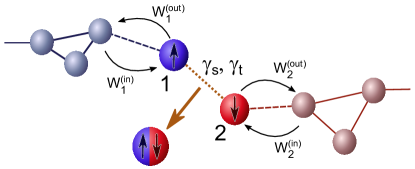
Figure 1: Electron-hole mechanism of OMAR. LUMO of molecules including the electron trapping site $1$ are shown with blue. HOMO including the hole trapping site $2$ are shown with red. Black arrows correspond to the rates of hopping to or from trapping sites. $\gamma_{s}$ and $\gamma_{t}$ are the rates of singlet and triplet exciton formation. The excitons never dissociate and recombine either radiatively or non-radiatively.

Both electron-hole and bipolaron mechanisms of OMAR are considered and the unified description for both the mechanisms is given when possible.

In the case of electron-hole mechanism the bottlenecks that control conductivity are considered to be the pairs of trapping sites for electron and hole (see Fig. 1). In such a pair the singlet exciton can be composed with the rate $\gamma_{s}$ and triplet one with the rate $\gamma_{t}$. After its generation the strong exchange interaction prevents exciton from changing its type. The singlet excitons then recombine radiatively. Triplet excitons recombine either due to phosphorescence Hoshino and Suzuki (1996); Baldo et al. (1998) or due to non-radiative processes. In the studied model the existing excitons do not affect the charge transport and formation of new excitons. The current $J$ through the bottleneck is proportional to the rate of exciton generation

$$J=e\gamma_{s}\frac{\overline{n_{1}n_{2}}-4\overline{s_{1}^{(\alpha)}s_{2}^{(\alpha)}}}{4}+e\gamma_{t}\frac{3\overline{n_{1}n_{2}}+4\overline{s_{1}^{(\alpha)}s_{2}^{(\alpha)}}}{4}$$ (1)

Here $\overline{n_{1}n_{2}}$ is the probability of the joint occupation of LUMO site $1$ with an electron and HOMO site $2$ with a hole. $\overline{s_{1}^{(\alpha)}s_{2}^{(\beta)}}$ is the averaged product of spin polarization on site $1$ along Cartesian direction $\alpha$ and spin polarization on site $2$ along the direction $\beta$. The sum over the repeating index $\alpha$ is assumed in Eq. (1).

Without average spin polarizations $\overline{s_{1}^{(\alpha)}s_{2}^{(\beta)}}$ describe the correlations of spin directions. They can be expressed in terms of spin density matrix $\rho_{s}$ as follows:

$$\overline{s_{1}^{(\alpha)}s_{2}^{(\beta)}}=\frac{1}{4}{\rm Tr}\left[\sigma_{1}^{(\alpha)}\sigma_{2}^{(\beta)}\rho_{s}\right]$$ (2)

Here $\sigma_{1}^{(\alpha)}$ is the Pauli matrix related to direction $\alpha$ and acting on the spin of trapping site $1$. $\sigma_{2}^{(\beta)}$ is the similar matrix for site $2$.

$\overline{s_{1}^{(\alpha)}s_{2}^{(\beta)}}$ are equal to zero in equilibrium because the temperature is large and $\rho_{s}$ is proportional to the identity matrix. It will be shown in Sec. III that $\overline{s_{1}^{(\alpha)}s_{2}^{(\beta)}}$ is proportional to $J$ and the current can be expressed as follows

$$J=e\gamma_{eh}(B)\overline{n_{1}n_{2}}$$ (3)

Here $\gamma_{eh}(B)$ is the effective exciton generation rate that depends on the applied magnetic field $B$.

The sites $1$ and $2$ are connected to other parts of the percolation cluster. The electron can be trapped on molecule $1$ with the rate $W_{1}^{(in)}$ and be released with rate $W_{1}^{(out)}$. $W_{2}^{(in)}$ and $W_{2}^{(out)}$ are similar rates for a hole to be trapped on site $2$ and leave it respectively (see Fig. 1 for the directions of hops corresponding to these rates). $W_{1,2}^{(in)}$ and $W_{1,2}^{(out)}$ are considered to be independent from magnetic field. It allows one to express magnetoresistance as a function of $\gamma_{eh}$. The corresponding derivations are provided in Appendix A. When the magnetoresistance is relatively small, it can be expressed as follows

$$\frac{R(B)-R(0)}{R(0)}=-\left\langle C_{eh}\frac{\gamma_{eh}(B)-\gamma_{eh}(0)}{\gamma_{eh}(0)}\right\rangle$$ (4)

Here $R(B)$ is the sample resistance, $\langle...\rangle$ describes the averaging over bottlenecks where exciton generation occurs. $C_{eh}$ is the constant that is derived in the Appendix A.

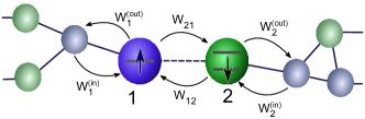
Figure 2: Bipolaron mechanism of OMAR. A-type LUMO are shown with blue color, B-type LUMO orbitals are shown with green color. Black arrows correspond to the rates of hopping to or from bottleneck.

The bipolaron mechanism of OMAR exists both in bipolar and unipolar devices. In this paper it is discussed for the unipolar devices with conductivity provided by electrons. It is assumed that LUMO can be double occupied by two electrons in spin-singlet state. The energy of double occupation is larger than the energy of single occupation by the Hubbard energy $E_{H}\gg T$. In this case all the molecular orbitals participating in hopping transport can de divided into the two types. The A-type orbitals can be unoccupied or single-occupied but are never double occupied due to the large Hubbard energy. The B-type orbitals have very low energy of single occupation and therefore are always occupied by at least one (resident) electron. Sometimes they are double occupied by electron pair in spin-singlet state. Note that both types of orbitals are LUMO.

The bottlenecks in the unipolar transport are the pairs of orbitals with the slowest hopping rates that are included into the percolation cluster. Only the pairs of LUMO with different types are important for the bipolaron mechanism of OMAR. Such a pair is shown in Fig. 2. I call the LUMO in bottleneck the hopping sites $1$ and $2$ with analogy to the trapping sites in electron-hole mechanism. The site $1$ corresponds to $A$-type molecular orbital and site $2$ has type $B$ for definiteness.

The current in the bottleneck can be expressed as follows

$$J=\frac{eW_{21}}{2}\left(\overline{n}_{1}-4\overline{s_{A}^{(\alpha)}s_{B}^{(\alpha)}}-\overline{n_{1}n_{2}}\right)\\ -2eW_{12}\overline{n_{2}(1-n_{1})}$$ (5)

Here $\overline{n_{1}n_{2}}$ is the probability of joint occupation. $W_{12}$ and $W_{21}$ are the rates of hops inside the bottleneck as shown in Fig. 2. Similarly to the electron-hole mechanism it will be shown that $\overline{s_{1}^{(\alpha)}s_{2}^{(\alpha)}}$ is proportional to the current $J$. It allows to express $J$ as follows

$$J=\kappa_{bp}(B)J_{0},$$ (6)

$$J_{0}=\frac{eW_{21}}{2}\overline{n_{1}(1-n_{2})}-2eW_{12}\overline{n_{2}(1-n_{1})}$$ (7)

Here $\kappa_{bp}(B)$ is the probability of electron to be transferred through the critical pair. It depends on the applied magnetic field leading to OMAR. When $|\kappa_{bp}(B)-\kappa_{bp}(0)|\ll\kappa_{bp}(0)$ the magnetoresistance can be expressed as follows

$$\frac{R(B)-R(0)}{R(0)}=-\left\langle\frac{\kappa_{bp}(B)-\kappa_{bp}(0)}{\kappa_{bp}(0)}\right\rangle$$ (8)

III Spin dynamics

In this section the dynamic of spin and spin correlations in the bottlenecks is described. The temperature is considered to be large compared to Zeeman energy of electron spins, energy of the hyperfine interaction and exchange energy, therefore in the equilibrium there is no spin polarization or correlations of spin directions. The spin correlations appear in the non equilibrium processes. For example if OMAR is controlled by electron-hole mechanism and the singlet exciton formation is more probable than the formation of triplet exciton, the triplet state of electron-hole pair in the bottleneck would be more probable than the singlet state. I assume that when electrons and holes leave the bottleneck sites to the percolation cluster they mix with other electrons and holes and the spin correlation is forgotten. It leads to an effective spin relaxation. Finally the spin correlations have coherent dynamics in the bottleneck due to hyperfine interaction with atomic nuclei and exchange interaction.

The kinetics of spin correlations can be expressed as follows:

$$\frac{d\overline{s_{1}^{(\alpha)}s_{2}^{(\beta)}}}{dt}=\frac{i}{\hbar}\overline{[H,s_{1}^{(\alpha)}s_{2}^{(\beta)}]}\\ +G\delta_{\alpha\beta}-R_{\alpha\beta;\alpha^{\prime}\beta^{\prime}}\overline{s_{1}^{(\alpha^{\prime})}s_{2}^{(\beta^{\prime})}}$$ (9)

Here the first term in r.h.s. describes the coherent spin dynamics due to hyperfine interaction with atomic nuclei, external magnetic field and the exchange interaction. $H$ is the Hamiltonian that includes all these energies. $G\delta_{\alpha\beta}$ stands for the generation of spin correlations due to the non-equilibrium processes. $R_{\alpha\beta;\alpha^{\prime}\beta^{\prime}}$ describes the relaxation of spin correlations due to electron transfer between bottleneck and other parts of the percolation cluster. $R_{\alpha\beta;\alpha^{\prime}\beta^{\prime}}$ also includes some contribution to relaxation of spin correlations due to the incoherent processes inside the bottleneck.

In the bipolaron mechanism the generation of spin correlations is proportional to the current

$$G=\frac{J}{4e}$$ (10)

and the relaxation is described with the expression

$$R_{\alpha\beta;\alpha^{\prime}\beta^{\prime}}=\left(W_{1}^{(out)}+W_{2}^{(in)}\right)\delta_{\alpha\alpha^{\prime}}\delta_{\beta\beta^{\prime}}\\ +\frac{W_{21}}{2}(\delta_{\alpha\alpha^{\prime}}\delta_{\beta\beta^{\prime}}-\delta_{\alpha\beta^{\prime}}\delta_{\beta\alpha^{\prime}}).$$ (11)

This expression shows that spin correlation is forgotten when electron leaves $A$-type site $1$ to the percolation cluster. The existence of the correlation assumes that $B$-type site $2$ is single occupied. It cannot lose its last electron. However, the correlation is forgotten when the second electron comes to site $2$ from the percolation cluster while the site $1$ is occupied. The hops from site $1$ to site $2$ are possible only in the singlet state of the spins. Even without net current it leads to the relaxation of coherent combination of singlet and triplet states Shumilin (2020). It is shown by the second term in r.h.s of Eq. (11).

In the electron-hole mechanism of OMAR the spin correlations appear due to the different rates of singlet and triplet exciton formation

$$G=(\gamma_{s}-\gamma_{t})\frac{\overline{n_{1}n_{2}}-4\overline{s_{1}^{(\gamma)}s_{2}^{(\gamma)}}}{16}.$$ (12)

Note that the probability of exciton decomposition is neglected, therefore the formation of exciton is possible only out of equilibrium. The relaxation of correlations for the electron hole mechanism of OMAR can be described as follows

$$R_{\alpha\beta;\alpha^{\prime}\beta^{\prime}}=(W_{1}^{(out)}+W_{2}^{(out)}+\gamma_{t})\delta_{\alpha\alpha^{\prime}}\delta_{\beta\beta^{\prime}}+\\ \gamma_{s}(\delta_{\alpha\alpha^{\prime}}\delta_{\beta\beta^{\prime}}-\delta_{\alpha\beta^{\prime}}\delta_{\beta\alpha^{\prime}}).$$ (13)

This expression shows that the correlation is forgotten when electron leaves site 1 or hole leaves site 2 to the percolation cluster. It is also transferred to the exciton in the process of triplet exciton formation. The singlet exciton formation is similar to the hop from $A$-type site to $B$-type site in the bipolaron mechanism and leads to the relaxation of the coherent combinations of singlet and triplet states.

The hamiltonian $H$ can be expressed with the same equation for both the OMAR mechanisms.

$$H=H_{B}+E_{ex}{\bf s}_{1}{\bf s}_{2}$$ (14)

Here $E_{ex}$ is the energy of exchange interaction of electron (or hole) spins on sites $1$ and $2$. $H_{B}$ describes the spin interaction with external magnetic field and atomic nuclei

$$H_{B}=\mu_{b}g\left({\bf B}+{\bf B}_{hf}^{(1)}\right){\bf s}_{1}+\mu_{b}g\left({\bf B}+{\bf B}_{hf}^{(2)}\right){\bf s}_{2}$$ (15)

Here ${\bf B}$ is the external magnetic field. ${\bf B}_{hf}^{(1)}$ and ${\bf B}_{hf}^{(2)}$ are the so-called hyperfine fields that describe hyperfine interaction with atomic nuclei on sites $1$ and $2$ respectively. It is presumed that on different sites the carrier spins interact with different nuclei, therefore ${\bf B}_{hf}^{(1)}$ and ${\bf B}_{hf}^{(2)}$ are independent. The distribution density of hyperfine fields is

$${\cal F}\left({\bf B}_{hf}^{(1,2)}\right)=\frac{1}{(\sqrt{2\pi}\Delta_{hf})^{3}}\exp\left(-\frac{\left|{\bf B}_{hf}^{(1,2)}\right|^{2}}{2\Delta_{hf}^{2}}\right)$$ (16)

Here $\Delta_{hf}\sim 10\,{\rm mT}$ is the typical hyperfine field. The description of hyperfine interaction with static hyperfine field corresponds to the limit of many nuclear spins interacting with a single electron spin.

The interaction with external and hyperfine fields leads to precession of electron and hole spins with frequencies ${\bm{\Omega}}_{1,2}=\mu_{b}g({\bm{B}}+{\bm{B}}_{hf}^{(1,2)})/\hbar$ related to sites $1$ and $2$

$$\frac{i}{\hbar}\overline{[H_{B},s_{1}^{(\alpha)}s_{2}^{(\beta)}]}=\epsilon_{\alpha\gamma\alpha^{\prime}}\Omega_{1}^{(\gamma)}\overline{s_{1}^{(\alpha^{\prime})}s_{2}^{(\beta)}}\\ +\epsilon_{\beta\gamma\beta^{\prime}}\Omega_{2}^{(\gamma)}\overline{s_{1}^{(\alpha)}s_{2}^{(\beta^{\prime})}}$$ (17)

The spin dynamics due to the exchange interaction can be described with the expression

$$\frac{i}{\hbar}E_{ex}\overline{[{\bf s}_{1}{\bf s}_{2},s_{1}^{(\alpha)}s_{2}^{(\beta)}]}=\\ \frac{1}{4}\frac{E_{ex}}{\hbar}\epsilon_{\alpha\beta\gamma}\left(\overline{s_{1}^{(\gamma)}s_{2}^{(0)}}-\overline{s_{1}^{(0)}s_{2}^{(\gamma)}}\right)$$ (18)

Here $\overline{s_{1}^{(0)}s_{2}^{(\gamma)}}$ describes the polarization of site $2$ in the direction $\gamma$ while the site $1$ is single occupied.

$$\overline{s_{1}^{(0)}s_{2}^{(\gamma)}}=\frac{1}{2}{\rm Tr}\left[\sigma_{1}^{(0)}\sigma_{2}^{(\gamma)}\rho_{s}\right]$$ (19)

which is similar to Eq. (2). $\sigma^{(0)}_{1}$ is the unit matrix that acts on single occupied states of site $1$. Therefore $s_{1}^{(0)}$ and $s_{2}^{(0)}$ are the operators of single occupation of sites $1$ and $2$ respectively.

For the electron-hole mechanism or for A-type sites in the bipolaron mechanism the “single occupation” and “occupation” are the same and $s_{1,2}^{(0)}=n_{1,2}$. In the considered model of bipolaron mechanism site $2$ is a $B$-type site and in this case $s_{2}^{(0)}=1-n_{2}$ because it is single-occupied when the second electron is absent. In what follows the notation $s_{1,2}^{(0)}$ is used when single-occupation is important for spin degrees of freedom, and $n_{1,2}$ is used for the description of current.

It is often assumed that statistics of spins is conserved when all the spins are reversed. If that would be the case $\overline{s_{1}^{(\gamma)}s_{2}^{(0)}}$ and $\overline{s_{1}^{(0)}s_{2}^{(\gamma)}}$ should be equal to zero. However, it will be shown that due to the exchange interaction even small external field $\sim 10-100\,{\rm mT}$ breaks the time reversal symmetry and leads to spin polarization in non-equilibrium conditions. To show it the kinetic equations for $\overline{s_{1}^{(\gamma)}s_{2}^{(0)}}$, $\overline{s_{1}^{(0)}s_{2}^{(\gamma)}}$ and the spin polarizations $\overline{s}_{1}^{(\alpha)}$, $\overline{s}_{1}^{(\alpha)}$ should be given.

I start from the expressions for spin polarizations in the electron-hole mechanism

$$\frac{d}{dt}\overline{s}_{1}^{(\alpha)}=-\frac{E_{ex}}{\hbar}\epsilon_{\alpha\beta\gamma}\overline{s_{1}^{(\beta)}s_{2}^{(\gamma)}}+\epsilon_{\alpha\beta\gamma}\Omega_{1}^{(\beta)}\overline{s_{1}^{(\gamma)}}-W_{1}^{(out)}\overline{s}_{1}^{(\alpha)}-\\ \gamma_{t}\overline{s_{1}^{(\alpha)}s_{2}^{(0)}}+\gamma_{s}\left(\overline{s_{1}^{(0)}s_{2}^{(\alpha)}}-\overline{s_{1}^{(\alpha)}s_{2}^{(0)}}\right),$$ (20)

$$\frac{d}{dt}\overline{s}_{2}^{(\alpha)}=\frac{E_{ex}}{\hbar}\epsilon_{\alpha\beta\gamma}\overline{s_{1}^{(\beta)}s_{2}^{(\gamma)}}+\epsilon_{\alpha\beta\gamma}\Omega_{2}^{(\beta)}\overline{s_{2}^{(\gamma)}}-W_{2}^{(out)}\overline{s}_{2}^{(\alpha)}-\\ \gamma_{t}\overline{s_{1}^{(0)}s_{2}^{(\alpha)}}+\gamma_{s}\left(\overline{s_{1}^{(\alpha)}s_{2}^{(0)}}-\overline{s_{1}^{(0)}s_{2}^{(\alpha)}}\right).$$ (21)

The first term in r.h.s. of Eqs. (20,21) describes the mutual precession of spins with frequency $E_{ex}/\hbar$. The second term stands for the spin precession in local fields. The third one shows that the spin polarization is lost when the electron or hole leaves the critical pair. The electron and hole spins can also be lost due to the formation of spin-polarized triplet exciton with the rate $\gamma_{t}$. Note that the recombination of the spin on site $1$ requires the hole on site $2$ therefore the relaxation of spin on site $1$ is proportional to $\overline{s_{1}^{(\alpha)}s_{2}^{(0)}}$. The singlet exciton formation cannot relax total spin but leads to re-distribution of spin polarization between the sites with the rate $\gamma_{s}$.

When the bipolaron mechanism is considered, $1\rightarrow 2$ hop is an analogue of the singlet exciton formation and $\gamma_{s}$ should be substituted with $W_{21}/2$. There is no analogue of triplet exciton formation in the bipolaron mechanism and $\gamma_{t}$ should be substituted with zero in Eqs. (20,21). Also $W_{2}^{(out)}$ should be substituted with $W_{2}^{(in)}$ in Eq. (21) because $B$-type site cannot lose it last electron but loses its spin polarization when it becomes double occupied.

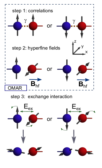
Figure 3: The three steps that lead to spin polarization of electrons and holes on the trapping sites. At the first step the spins become correlated due to the different rates of singlet and triplet exciton formation. At the second step the correlations are modified due to spin precession in effective on-site fields. It is shown with 90 degree rotation of the hole spin around x-axis. The modified correlations correspond to the coherent combination of singlet and triplet states. At the third step the spin polarization precess around the direction of the total spin. Initial rotation directions and the spin directions after 90 degree rotation are shown. Spin polarization along $x$ axis of both electron and hole (averaged over left and right sides of the picture) appears.

Note that the exchange interaction leads to spin polarization only when $\overline{s_{1}^{(\alpha)}s_{2}^{(\beta)}}-\overline{s_{1}^{(\beta)}s_{2}^{(\alpha)}}\neq 0$. Such correlations correspond to the coherent combination of singlet and triplet states of the electron-hole pair. Therefore the overall picture of dynamic spin polarizations can be described with the three steps that are shown in Fig. 3. At the first step the probabilities of singlet and triplet states of polaron pair become non-equilibrium due to the different rates of singlet and triplet exciton formation or due to the current and double occupation possibility. It means that spins of the carriers become correlated. In Fig. 3 it is schematically shown with both the spins directed either up or down. It is important that electron and hole spin polarizations averaged over left and right side of the figure are zero.

At the second step the spin precession with different frequencies ${\bm{\Omega}}_{1}$ and ${\bm{\Omega}_{2}}$ leads to a coherent combination of singlet and triplet states and to the correlations with $\overline{s_{1}^{(\alpha)}s_{2}^{(\beta)}}-\overline{s_{1}^{(\beta)}s_{2}^{(\alpha)}}\neq 0$. In Fig. 3 it is schematically shown with 90 degree rotation of hole spin on site 2 around $x$-axis. These two steps are common for the theory of OMAR.

At the third step exchange interaction leads to mutual precession of spins, or, which is the same, to precession of spins ${\bf s}_{1}$ and ${\bf s}_{2}$ around the direction of ${\bf s}_{1}+{\bf s}_{2}$. In Fig. 3 the initial direction of this precession is shown together with the result of such a precession over angle $\pi/2$. The electron has negative polarization in $x$ direction both on the left and on the right side of the figure. It means that averaged electron spin polarization appears.

At this point the polarizations of electron and hole are opposite because the first terms in r.h.s. of Eq. (20) and Eq. (21) have equal absolute values and different signs. However, other terms in r.h.s. of Eqs. (20,21) are different and the precession of spins with different frequencies $\bm{\Omega}_{1}$ and $\bm{\Omega}_{2}$ and different rates of electron and hole spin relaxation lead to non-zero averaged spin $\overline{\bf s}_{1}+\overline{\bf s}_{2}$. It appears that usually after the averaging over hyperfine fields the spin polarization on sites $1$ and $2$ have the same direction.

The kinetic equations for $\overline{s_{1}^{(\alpha)}s_{2}^{(0)}}$ and $\overline{s_{1}^{(0)}s_{2}^{(\alpha)}}$ are similar to the equations for $\overline{s}_{1}^{(\alpha)}$ and $\overline{s}_{1}^{(\alpha)}$. However the terms describing the transitions of electrons and holes between the bottleneck and other parts of the percolation cluster are different

$$\frac{d}{dt}\overline{s_{1}^{(\alpha)}s_{2}^{(0)}}=-\frac{E_{ex}}{\hbar}\epsilon_{\alpha\beta\gamma}\overline{s_{1}^{(\beta)}s_{2}^{(\gamma)}}+\epsilon_{\alpha\beta\gamma}\Omega_{1}^{(\beta)}\overline{s_{1}^{(\gamma)}s_{2}^{(0)}}\\ -(W_{1}^{(out)}+W_{2}^{(out)}+W_{2}^{(in)}+\gamma_{t})\overline{s_{1}^{(\alpha)}s_{2}^{(0)}}\\ +W_{2}^{(in)}\overline{s}_{1}^{(\alpha)}+\gamma_{s}\left(\overline{s_{1}^{(0)}s_{2}^{(\alpha)}}-\overline{s_{1}^{(\alpha)}s_{2}^{(0)}}\right),$$ (22)

$$\frac{d}{dt}\overline{s_{1}^{(0)}s_{2}^{(\alpha)}}=\frac{E_{ex}}{\hbar}\epsilon_{\alpha\beta\gamma}\overline{s_{1}^{(\beta)}s_{2}^{(\gamma)}}+\epsilon_{\alpha\beta\gamma}\Omega_{2}^{(\beta)}\overline{s_{1}^{(0)}s_{2}^{(\gamma)}}-\\ (W_{2}^{(out)}+W_{1}^{(in)}+W_{1}^{(out)}+\gamma_{t})\overline{s_{1}^{(0)}s_{2}^{(\alpha)}}\\ +W_{1}^{(in)}\overline{s}_{2}^{(\alpha)}+\gamma_{s}\left(\overline{s_{1}^{(\alpha)}s_{2}^{(0)}}-\overline{s_{1}^{(0)}s_{2}^{(\alpha)}}\right).$$ (23)

To consider the bipolaron mechanism one should substitute $\gamma_{s}$ with $W_{21}/2$, $\gamma_{t}$ with zero and mutually exchange $W_{2}^{(in)}$ and $W_{2}^{(out)}$.

Eqs. (9-23) compose a system of 21 linear equations that should be solved under stationary conditions together with Eqs. (1 - 5) that describe electric current and exciton generation. However, in any case all the spin correlations and polarizations are proportional to $G$. Therefore it is possible to express $\sum_{\alpha}\overline{s_{1}^{\alpha}s_{2}^{\alpha}}={\cal T}_{s}G$ where ${\cal T}_{s}$ has the dimensionality of time. It allows one to use Eqs. (3,6).

In the electron-hole mechanism the rate $G$ of generation of spin correlation can be expressed in terms of ${\cal T}_{s}$ as follows

$$G=\frac{1}{16}\frac{(\gamma_{s}-\gamma_{t})\overline{n_{1}n_{2}}}{1+{\cal T}_{s}(\gamma_{s}-\gamma_{t})/4}$$ (24)

Its substitution to Eq. (1) leads to Eq. (3) with

$$\gamma_{eh}=\gamma_{t}+\frac{(\gamma_{s}-\gamma_{t})}{4+{\cal T}_{s}(\gamma_{s}-\gamma_{t})}.$$ (25)

In the bipolaron mechanism the similar arguments lead to the expression

$$\kappa_{bp}=\frac{1}{1+W_{21}{\cal T}_{s}/2}.$$ (26)

IV Exciton formation rate and organic magnetoresistance

Exchange interaction modifies the shape of OMAR and the dependence of the exciton formation rate $\gamma_{eh}$ on applied magnetic field $B$. It can help to identify the situations when dynamic spin polarization occurs in organic semiconductor. Magnetoresistance and $\gamma_{eh}(B)$ dependence are related in the considered model in the electron-hole mechanism due to Eq. (4). The shape of OMAR in the bipolaron mechanism has similar properties. Therefore only the shape of $\gamma_{eh}(B)$ dependence is considered in this section for definiteness.

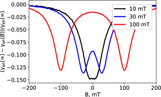
Figure 4: The shape of $\gamma_{eh}(B)$ dependence with different exchange fields $B_{ex}$ shown in legend.

The exciton formation rate is calculated with numeric solution of Eqs. (9 - 23). The typical value of hyperfine field $\Delta_{B}=10\,{\rm mT}$ is considered. The exchange interaction significantly modify OMAR when the “exchange field” $B_{ex}=E_{ex}/g\mu_{b}$ is larger or comparable with the hyperfine field $B_{ex}\gtrsim\Delta_{B}$. Therefore the values of $B_{ex}$ from $10$ to $100\,{\rm mT}$ are discussed in this section.

In Fig. 4 the calculated dependence $\gamma_{eh}(B)$ is shown. It is compared to the value $\gamma_{eh}(\infty)$ in high magnetic fields where the exciton generation rate is saturated. The singlet and triplet exciton formation rates are considered to be $\gamma_{s}=20\,{\rm\mu s}^{-1}$ and $\gamma_{t}=4\,{\rm\mu s}^{-1}$ respectively. These rates are $\sim 10$ times slower than the spin precession in the hyperfine field. The transitions of electrons and holes between the sites $1$ and $2$ and the rest of percolation cluster are described with the rates $W_{1}^{(in)}=30\,{\rm\mu s}^{-1}$, $W_{2}^{(in)}=100\,{\rm\mu s}^{-1}$, $W_{1}^{(out)}=5\,{\rm\mu s}^{-1}$, $W_{2}^{(out)}=1\,{\rm\mu s}^{-1}$. The relatively small values $W_{1}^{(out)}$ and $W_{2}^{(out)}$ show that the sites $1$ and $2$ are effective traps for electron and hole respectively. These parameters were considered to be the same for all the bottlenecks that control the transport. The averaging was made over $10^{4}$ random values of hyperfine fields ${\bf B}_{hf}^{(1)}$ and ${\bf B}_{hf}^{(2)}$.

The exchange interaction splits zero-field peak of $\gamma_{eh}(B)$ dependence. This splitting is small when ${B_{ex}\lesssim\Delta_{B}}$. This results qualitatively agrees with the calculations made in Ref. Nguyen et al. (2012) where it was compared with magnetoresistance measured in $\rm Alq_{3}$. When the exchange interaction is strong $B_{ex}\gtrsim 10\Delta_{B}$, $\gamma_{eh}(B)$ shape consists of two peaks at $B=\pm B_{ex}$. It can be explained with the following model (Fig. 5). At zero magnetic field the exchange interaction prevents the hyperfine interaction from mixing singlet and triplet states. In this case the hyperfine interaction does not affect the exciton formation and current. However the energy of singlet state $E_{s}$ does not depend of magnetic field while the energy of one of the triplet states $E_{t-}$ decreases with $B$. When $|B-B_{ex}|\lesssim\Delta_{hf}$, the singlet-triplet mixing due to hyperfine field becomes effective. It leads to the peak in $\gamma_{eh}(B)$ dependence.

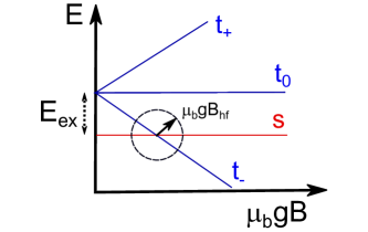
Figure 5: Energies of the triplet and singlet spin states in magnetic field. The circle shows where the hyperfine interaction can efficiently mix the states.

To the best of the authors knowledge such a resonance OMAR shape was never observed in experiment. However, it appears because the exchange interaction is considered to be the same for all the bottlenecks that control exciton formation. In organic semiconductor the inter-molecular exchange interaction has strong dependence on the overlap integrals that have the exponentially-broad distribution Massé et al. (2017). Therefore, one can expect the broad distribution of exchange energies. In real materials it should be determined with numeric simulation. Here I consider only a simplified model that shows that exchange energy $E_{ex}$ in the bottleneck can vary in order of magnitude

$$B_{ex}=B_{ex}^{(0)}\exp(-\xi)$$ (27a)

$${\cal F}_{\xi}(\xi)=\frac{1}{\xi_{max}},\quad\xi\in(0,\xi_{max})$$ (27b)

The exchange field is always smaller than $B_{ex}^{(0)}$. The value $\xi$ describes its suppression due to the small overlap integral between sites $1$ and $2$. The distribution density ${\cal F}_{\xi}$ of the suppression factor is flat between zero and $\xi_{max}$ that is the maximum suppression that still allows efficient exciton generation. The shape of $\gamma_{eh}(B)$ dependence for $B_{ex}^{(0)}=1T$ and $\xi_{max}=4$ and $8$ is shown in Fig. 6. The splitting of the peak is controlled by the smallest possible exchange energies. When $B_{ex}^{(0)}\exp(-\xi_{max})$ is large compared to $\Delta_{B}$ the splitting is clearly observable while for $B_{ex}^{(0)}\exp(-\xi_{max})<\Delta_{B}$ it is suppressed and $\gamma_{eh}(B)$ dependence has Lorentz shape.

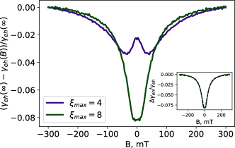
Figure 6: $\gamma_{eh}(B)$ dependence with the distribution of exchange fields described by Eqs. (27) with different $\xi_{max}$ described in legend. The inset shows the comparison between the results for $\xi_{max}=8$ (green curve) and Lorentz function $\gamma_{eh}(\infty)-\gamma_{eh}(B)\propto B^{2}/(B^{2}+B_{0}^{2})$ with $B_{0}=45\,{\rm mT}$ (black dashed curve).

V dynamic spin polarization

In the presence of exchange interaction the non-equilibrium phenomena that lead to OMAR also yield the spin-polarizations of electrons and holes in the bottleneck. It can be understood from non-zero values of $d\overline{s}_{1}^{(\alpha)}/dt$ and $d\overline{s}_{2}^{(\alpha)}/dt$ in Eqs. (20,21). The relative polarizations on sites $1$ and $2$ are defined as $P_{1}$ and $P_{2}$ respectively.

$$P_{1}=\frac{2\overline{s}_{1}^{(z)}}{\overline{s}_{1}^{(0)}},\quad P_{2}=\frac{2\overline{s}_{2}^{(z)}}{\overline{s}_{2}^{(0)}}.$$ (28)

The polarizations are normalized to the single occupation probabilities of sites $1$ and $2$. The averaged polarization is always directed along the axis of the applied magnetic field.

In the electron-hole mechanism of OMAR the produced triplet excitons are also spin-polarized and their polarization is

$$P_{ex}=\frac{\overline{s_{1}^{(z)}s_{2}^{(0)}}+\overline{s_{1}^{(0)}s_{2}^{(z)}}}{\overline{n_{1}n_{2}}}.$$ (29)

In both of the OMAR mechanisms spin current appears. It is different for the two parts of the percolation cluster connected to sites $1$ and $2$ because the spin is not conserved in the bottleneck. I assume that the electrons that come from the percolation cluster to the bottleneck are not spin-polarized. It leads to the following expressions for spin currents $J_{s}^{(1)}$ and $J_{s}^{(2)}$ in the bipolaron mechanism

$$J_{s}^{(1)}=W_{1}^{(out)}\overline{s}_{1}^{(z)},\quad J_{s}^{(2)}=-W_{2}^{(in)}\overline{s}_{2}^{(z)}.$$ (30)

The similar expressions for the spin currents in the electron-hole mechanism are

$$J_{s}^{(1)}=W_{1}^{(out)}\overline{s}_{1}^{(z)},\quad J_{s}^{(2)}=-W_{2}^{(out)}\overline{s}_{2}^{(z)}.$$ (31)

Because the spin currents are directly related to spin polarizations, I discuss only $P_{1}$, $P_{2}$ and $P_{ex}$. In this section the spin polarizations are calculated numerically under stationary conditions for the systems described in Sec. IV. In Fig. 7(a) magnetic field dependence of $P_{1}$, $P_{2}$ and $P_{ex}$ is shown for the exchange field $B_{ex}=30\,{\rm mT}$ and the other conditions corresponding to Fig. 4. The polarizations almost coincide in this situation. Some details about their coincidence are given in Sec. VI. Note that although the signs of $d\overline{s}_{1}^{(\alpha)}/dt$ and $d\overline{s}_{2}^{(\alpha)}/dt$ in Eqs. (20,21) are different when spin polarizations are zero, the resulting polarizations that take into account the spin transfer between molecules and (most important) the averaging over the hyperfine fields have the same sign. Inset in Fig. 7(a) shows the typical spin polarizations $P_{1}$ and $P_{2}$ without the averaging over hyperfine fields. They have the same sign when $B$ is close to $\pm B_{ex}$ and different signs otherwise.

Fig. 7(b) shows the triplet exciton polarization at different exchange fields. The shape of the dependence $P_{ex}(B)$ is almost independent of $B_{ex}$ when $B_{ex}\leq\Delta_{hf}$ while its amplitude grows with $B_{ex}$. For large exchange energy the shape of the dependence contains the two peaks at $B=\pm B_{ex}$ in agreement with Fig. 5.

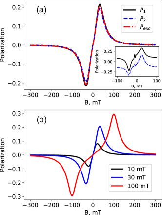
Figure 7: Dynamic spin polarization calculated numerically and averaged over $10^{4}$ hyperfine fields. (a) the spin polarization of electrons on site $1$, holes on site $2$ and triplet excitons for the exchange field $B_{ex}=30\,{\rm mT}$. The inset shows the typical spin polarizations without averaging over hyperfine fields. (b) The triplet exciton spin polarization at different exchange fields shown in legend.

The results for the broad distribution of exchange energies described with Eq. (27) are shown in Fig. 8. Similarly to $\gamma_{eh}(B)$ dependence shown in Fig. 6 the peaks in the dependence of polarization on the applied field are smeared due to the distribution of the exchange energies. However, even when the splitting of zero-field peak in $\gamma_{eh}(B)$ dependence is hardly observable (as it is in the case of $\xi_{max}=8$) the spin polarization is not completely suppressed. The splitting of the zero-field peak depends on the minimal possible exchange energy while the spin polarization in magnetic field $B$ depends on the probability for the exchange field to be $B_{ex}\sim B$.

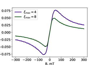
Figure 8: Dynamic polarization with the broad distribution of exchanged field described by Eq. (27) with $\xi_{max}$ shown in legend.

VI Spin polarization in resonance

The results of numeric simulation provided in Sec. V show that spin polarization is the strongest in the “resonance situation” when $B=B_{ex}\gg B_{hf}$. This situation is studied in details in this section. The electron-hole mechanism of OMAR is considered for definiteness.

To further simplify the theory I assume that singlet exciton formation rate is fast $\gamma_{s}\gg W_{1}^{(in)}+W_{1}^{(out)}+W_{2}^{(in)}+W_{2}^{(out)}$ and triplet exciton formation rate is very slow $\gamma_{t}\ll W_{1}^{(out)}+W_{2}^{(out)}$. The spin precession in hyperfine field is fast compared to hops and exciton formation rates $\mu_{b}gB_{hf}\gg\hbar\gamma_{s}$.

The singlet electron-hole pair forms exciton almost immediately after it appears. The electron-hole pair in the state $t_{-}$ can easily change its state to singlet and also form a singlet exciton. However the pairs in states $t_{+}$ and $t_{0}$ usually dissociate due to electron and hole leaving the sites $1$ and $2$. Sometimes, however, such a pair forms a triplet exciton due to the finite rate $\gamma_{t}$. Even at this point it is clear that the triplet excitons are strongly spin-polarized because no $t_{-}$ triplet excitons appear.

These assumptions allow to reduce the system (9 - 23) for 21 “spin variables” and the joint equations for “charge” variables $\overline{n}_{1}$, $\overline{n}_{2}$ and $\overline{n_{1}n_{2}}$ to the system of six linear equations. The new equations describe the system in terms of the following variables. $p_{+}$ and $p_{0}$ are the probabilities for the bottleneck to be occupied by the electron-hole pair in $t_{+}$ and $t_{0}$ states respectively. The probabilities of the bottleneck to be occupied by electrons and holes in singlet or $t_{-}$ states are neglected due to the fast singlet exciton generation rate and effective coupling between singlet and $t_{-}$ state. $p_{1}$ and $p_{2}$ are the probabilities for the occupation of sites $1$ and $2$ respectively while the second site is unoccupied. $p_{1s}$ is the difference between the probabilities for site $1$ to be occupied by spin-up and spin down electron while the site $2$ is empty. $p_{2s}$ is the similar quantity for the site $2$.

Polarizations $P_{1}$, $P_{2}$ and $P_{ex}$ are expressed in these notations as follows

$$P_{ex}=\frac{p_{+}}{p_{+}+p_{0}},$$ (32a)

$$P_{1}=\frac{p_{+}+p_{1s}}{p_{+}+p_{0}+p_{1}},\quad P_{2}=\frac{p_{+}+p_{2s}}{p_{+}+p_{0}+p_{2}}.$$ (32b)

Eqs. (32) show that triplet exciton polarization is related only to the states when both the sites of the bottleneck are occupied, while the polarizations $P_{1}$ and $P_{2}$ are also affected by states when only one of the sites is occupied.

The system of equations for $p_{\zeta}$ where $\zeta=+,0,1,2,1s,2s$ follows from the stationary conditions $dp_{\zeta}/dt=0$. The stationary conditions for $p_{+}$ yields

$$\frac{p_{1}+p_{1s}}{4}W_{2}^{(in)}+\frac{p_{2}+p_{2s}}{4}W_{1}^{(in)}\\ =(W_{1}^{(out)}+W_{2}^{(out)})p_{+}$$ (33)

The electron-hole pair in $t_{+}$ state can appear when electron or hole is trapped on the corresponding site of the bottleneck while the second site is occupied. When the occupied site is not spin-polarized (for example when $p_{1}=1$, $p_{1s}=0$ and the hole becomes trapped on site $2$) any of the four spin states of electron-hole pair appears with equal probability. When the site is fully spin-polarized ($p_{1}=p_{1s}=1$) the probability of $t_{+}$ state after the hole trapping is $1/2$. The electron-hole pair dissociates when electron or hole leaves the bottleneck. The probability of triplet exciton formation $\gamma_{t}$ is neglected in comparison to $W_{1}^{(out)}+W_{2}^{(out)}$.

The probability of appearance of $t_{0}$ state is not affected by spin polarization of trapping sites leading to the stationary condition for $p_{0}$

$$\frac{p_{1}}{4}W_{2}^{(in)}+\frac{p_{2}}{4}W_{1}^{(in)}=(W_{1}^{(out)}+W_{2}^{(out)})p_{0}$$ (34)

The stationary conditions for the probabilities $p_{1}$ and $p_{2}$ lead to the equations

$$W_{2}^{(out)}(p_{+}+p_{0})+W_{1}^{(in)}(1-p_{1}-p_{2}-p_{+}-p_{0})\\ =(W_{1}^{(out)}+W_{2}^{(in)})p_{1}$$ (35a)

$$W_{1}^{(out)}(p_{+}+p_{0})+W_{2}^{(in)}(1-p_{1}-p_{2}-p_{+}-p_{0})\\ =(W_{2}^{(out)}+W_{1}^{(in)})p_{2}$$ (35b)

The stationary conditions for $p_{1s}$ and $p_{2s}$ read

$$W_{2}^{(out)}p_{+}=(W_{1}^{(out)}+W_{2}^{(in)})p_{1s}$$ (36a)

$$W_{1}^{(out)}p_{+}=(W_{2}^{(out)}+W_{1}^{(in)})p_{2s}$$ (36b)

The system of equations (33-36) can be solved analytically but the solution is quite cumbersome. Here it is given for the specific “symmetrical” case $W_{1}^{(in)}=W_{2}^{(in)}=W^{(in)}$, $W_{1}^{(out)}=W_{2}^{(out)}=W^{(out)}$. In this case $p_{1}=p_{2}$ and $p_{1s}=p_{s2}$. All the $p_{\zeta}$ are functions of the ratio $w=W^{(out)}/W^{(in)}$.

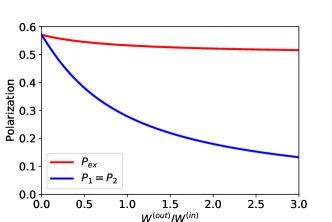
Figure 9: Spin polarizations $P_{ex}$, and $P_{1}=P_{2}$ under the resonance conditions.

The spin polarization $p_{1s}$ of the site $1$ is related to the triplet occupation number $p_{+}$ as follows

$$p_{1s}=\frac{wp_{+}}{w+1}$$ (37)

The triplet occupation probabilities are proportional to the probability $p_{1}$ of the occupation of a single site.

$$p_{0}=\frac{p_{1}}{4w},\quad p_{+}=\frac{p_{1}}{4w}\frac{1+w}{3/4+w}$$ (38)

The analytical expression for $p_{1}$ is

$$p_{1}=\frac{4w(4w+3)}{16w^{3}+52w^{2}+37w+7}$$ (39)

The spin polarizations $P_{1}$, $P_{2}$ and $P_{ex}$ than should be calculated from Eqs. (32). The result of such a calculation is shown in Fig. 9. When $W^{(in)}\gg W^{(out)}$ the polarizations $P_{1}=P_{2}$ and $P_{ex}$ coincide. Both of the trapping sites are almost always occupied and $p_{1}$ can be neglected in comparison to $p_{0}$ and $p_{+}$. $p_{+}$ is equal to $4p_{0}/3$ in this case leading to $P_{ex}=P_{1}=P_{2}=4/7$. It is the largest spin polarization possible in the discused model. Note that in Sec. V $W_{1}^{(in)}\gg W_{2}^{(out)}$ and $W_{2}^{(in)}\gg W_{2}^{(out)}$ were considered. Fig. 7 shows that polarizations $P_{1}$, $P_{2}$ and $P_{ex}$ coincide in this case even for non-resonance situation.

In the opposite limit $W^{(out)}\gg W^{(in)}$ the probabilities of $t_{+}$ and $t_{0}$ states are equal leading to $P_{ex}=1/2$. Polarizations $P_{1}$ and $P_{2}$ are small in this limit.

VII discussion

The dynamic spin polarization was observed in non-organic GaAs quantum dots due to the circular polarization of photoluminescence. It was possible due the strong spin-orbit intercation in GaAs that allows radiative recombination of excitons with angular momentum equal to unity. In organic semiconductors such a detection is not an easy task because usually only singlet excitons recombine radiatively. The radiative recombination of triplets in organic is called phosphorescence and can be achieved by the introduction of certain impurities (the so-called phosphors) to organic semiconductors. It makes the optical detection of dynamic spin polarization in organics possible at least in theory. However, such a detection is related to additional restrictions that are out of the scope of the provided model: the spin of a triplet exciton should be conserved during the transition to such a phosphor and the following recombination process.

However, organic semiconductors also have advantages over the quantum dots when dynamic spin polarization is considered. Spin-phonon interaction in non-organic semiconductors leads to fast spin relaxation that suppress circular polarization of luminescence in quantum dots at temperatures $T\gtrsim 10\,{\rm K}$ Smirnov et al. (2020). However, OMAR and strong spin-valve effect exist both at low and room temperatures due to the weak spin-orbit interaction in organic materials. It makes it possible for dynamic spin polarization to also exist at room temperature.

The long spin diffusion length measured in some organic semiconductors gives hope that the spin polarization can be detected in transport measurements in hybrid devices with ferromagnetic contacts. Another possibility is the muon spin rotation experiments that were able to detect spin-polarization in working spin-valve devices. Actually the author believes that it may be relevant to revisit organic spin-valve experiments in view of the results of this article. Usually only the two possibilities were considered for organic spin-valve: the spin is injected from the first ferromagnetic contact and is detected by the second one or the spin-valve is due to the tunneling through pin-holes in organic layer. Now the third assumption should be added: the spin can be generated inside organic layer. The external fields $\sim 100\,{\rm mT}$ required for such a generation can be related for example to fringe fields of magnetic contacts Wang et al. (2012).

The effective dynamic spin polarization requires exchange energies between electrons and holes on different molecules in the bottleneck to be larger or comparable with the energy of hyperfine interaction of electron and nuclear spins. The existing estimates of the exchange energy are quite controversial. In Nguyen et al. (2012) the value $B_{ex}=0.2\,{\rm mT}$ was extracted from the comparison of measured OMAR shape with theory. Such a value is clearly insufficient for the significant spin polarization. However such an estimate of the exchange energy can be complicated if $B_{ex}$ has broad distribution, as it follows from Fig. 6. The exchange interaction between electrons localized on different molecules was also invoked in Ref. Yu (2013) to describe the absence of Hanle effect in organic spin-valves. The exchange energies corresponding to $B_{ex}\gtrsim 0.1T$ where considered to be possible. Perhaps the typical exchange energies in organic semiconductor can be very different in different samples and depend not only on chemical structure but also on the concentration of injected charge carriers. The strong dynamic spin polarization can occur in the samples where the condition $B\sim B_{ex}\gtrsim B_{hf}$ is satisfied.

In conclusion it was shown that exchange interaction between electrons and holes localized on different molecules leads to spin polarization in organic semiconductors where OMAR is observed. For the polarization to be significant the exchange interaction should be comparable or larger than hyperfine interaction of electron and nuclear spins. The exchange interaction also modifies the shape of OMAR. However, such a modification can be masked by a broad distribution of exchange energies. This broad distribution does not completely suppress the spin polarization.

The author is grateful to D.S. Smirnov, V.V. Kabanov, V.I. Dediu and Y.M. Beltukov for many fruitful discussions. The support from Foundation for the Advancement of Theoretical Physics and Mathematics “Basis” is greatly acknowledged.

Appendix A Magnetoresistance in electron-hole mechanism

To calculate the magnetoresistance in electron-hole mechanism the current should be expressed as the rate of trapping in sites $1$ and $2$

$$J=e(1-\overline{n}_{1})W_{1}^{(in)}-eW_{1}^{(out)}\overline{n_{1}}$$ (40)

$$J=e(1-\overline{n}_{2})W_{2}^{(in)}-eW_{2}^{(out)}\overline{n_{2}}$$ (41)

Eq. (40) shows that the electron cannot be trapped on site $1$ if it is already occupied and that all the electrons that are trapped and do not leave site $1$ contribute to exciton generation and current. Eq. (41) is the similar expression for site $2$.

The current given by Eqs. (40,41) is equal to the current (3). This system of equation should be complemented by the master equation for joined occupation probability $\overline{n_{1}n_{2}}$

$$\frac{d}{dt}\overline{n_{1}n_{2}}=0=W_{1}^{(in)}\overline{n}_{2}+W_{2}^{(in)}\overline{n}_{1}\\ -\left[\widetilde{W}_{12}+\gamma_{eh}(B)\right]\overline{n_{1}n_{2}}$$ (42)

Here $\widetilde{W}_{12}=W_{1}^{(in)}+W_{1}^{(out)}+W_{2}^{(in)}+W_{2}^{(out)}$.

The solution of Eqs. (3, 40 - 42) yields the following expressions for $n_{1}$ and $n_{2}$:

$$\overline{n}_{1}=\frac{W_{1}^{(in)}-\widetilde{\gamma}\overline{n_{1}n_{2}}}{W_{1}^{C}}$$ (43)

$$\overline{n}_{2}=\frac{W_{2}^{(in)}-\widetilde{\gamma}\overline{n_{1}n_{2}}}{W_{2}^{C}}$$ (44)

Here $W_{1}^{C}=W_{1}^{(in)}+W_{1}^{(out)}$, $W_{2}^{C}=W_{2}^{(in)}+W_{2}^{(out)}$.

The current $J$ and joined occupation probability $\overline{n_{1}n_{2}}$ are expressed as follows:

$$J=\frac{e\gamma_{eh}W_{1}^{(in)}W_{2}^{(in)}\widetilde{W}_{12}}{W_{1}^{C}W_{2}^{C}\widetilde{W}_{12}+\gamma_{eh}{\cal W}}$$ (45)

$$\overline{n_{1}n_{2}}=\frac{W_{1}^{(in)}W_{2}^{(in)}\widetilde{W}_{12}}{W_{1}^{C}W_{2}^{C}\widetilde{W}_{12}+\gamma_{eh}{\cal W}}$$ (46)

Here ${\cal W}=W_{1}^{C}W_{2}^{C}+W_{1}^{C}W_{1}^{(in)}+W_{2}^{C}W_{2}^{(in)}$.

The magnetoresistance can be expressed as $(J(0)-J(B))/J(B)$. When the effect of spin correlations on conductivity is small, the magnetoresistance is also small ($|J(0)-J(B)|\ll J(0)$) and Eq. (4) can be derived from Eq. (45) with $C_{eh}$ equal to

$$C_{eh}=\frac{W_{1}^{C}W_{2}^{C}\widetilde{W}_{12}}{W_{1}^{C}W_{2}^{C}\widetilde{W}_{12}+\gamma_{eh}(0){\cal W}}$$ (47)

Here $\gamma_{eh}(0)$ is calculated in zero magnetic field.

References

- Forrest (2004) S. Forrest, Nature 428, 911 (2004).
- Wei et al. (2018) Q. Wei, N. Fei, A. Islam, T. Lei, L. Hong, R. Peng, X. Fan, L. Chen, P. Gao, and Z. Ge, Adv. Opt. Mat. 6, 1800512 (2018),
- Brabec et al. (2001) C. J. Brabec, N. S. Sariciftci, and J. C. Hummelen, Adv. Opt. Mat. 11, 15 (2001).
- Zhou et al. (2019) R. Zhou, Z. Jiang, C. Yang, J. Yu, J. Feng, M. A. Adil, D. Deng, W. Zou, J. Zhang, K. Lu, et al., Nat. Commun. 10, 5393 (2019)
- Qiu et al. (2020) B. Qiu, Z. Chen, S. Qin, J. Yao, W. Huang, L. Meng, H. Zhu, Y. M. Yang, Z.-G. Zhang, and Y. Li, Adv. Mat. 32, 1908373 (2020),
- Allard et al. (2008) S. Allard, M. Forster, B. Souharce, H. Thiem, and U. Scherf, Angewandte Chemie International Edition 47, 4070 (2008),
- Di et al. (2013) C.-a. Di, F. Zhang, and D. Zhu, Advanced Materials 25, 313 (2013),
- Xiong et al. (2004) Z. H. Xiong, D. Wu, Z. Valy Vardeny, and J. Shi, Nature 427, 821 (2004)
- Pramanik et al. (2007) S. Pramanik, C.-G. Stefanita, S. Patibandla, S. Bandyopadhyay, K. Garre, N. Harth, and M. Cahay, Nature Nanotechnology 2, 216 (2007)
- Drew et al. (2009) A. J. Drew, J. Hoppler, L. Schulz, F. L. Pratt, P. Desai, P. Shakya, T. Kreouzis, W. P. Gillin, A. Suter, N. A. Morley, et al., Nature Materials 8, 109 (2009),
- Dediu et al. (2009) V. A. Dediu, L. E. Hueso, I. Bergenti, and C. Taliani, Nature Materials 8, 707 (2009)
- Schmidt et al. (2000) G. Schmidt, D. Ferrand, L. W. Molenkamp, A. T. Filip, and B. J. van Wees, Phys. Rev. B 62, R4790 (2000),
- Prezioso et al. (2011) M. Prezioso, A. Riminucci, I. Bergenti, P. Graziosi, D. Brunel, and V. A. Dediu, Advanced Materials 23, 1371 (2011),
- Yu (2013) Z. G. Yu, Phys. Rev. Lett. 111, 016601 (2013),
- Grünewald et al. (2013) M. Grünewald, R. Göckeritz, N. Homonnay, F. Würthner, L. W. Molenkamp, and G. Schmidt, Phys. Rev. B 88, 085319 (2013),
- Kalinowski et al. (2003) J. Kalinowski, M. Cocchi, D. Virgili, P. Di Marco, and V. Fattori, Chem. Phys. Lett. 380, 710 (2003)
- Mermer et al. (2005) O. Mermer, G. Veeraraghavan, T. L. Francis, Y. Sheng, D. T. Nguyen, M. Wohlgenannt, A. Köhler, M. K. Al-Suti, and M. S. Khan, Phys. Rev. B 72, 205202 (2005),
- Prigodin et al. (2006) V. N. Prigodin, J. D. Bergeson, D. M. Lincoln, and A. J. Epstein, Synthetic Metals 156, 757 (2006),
- Bobbert et al. (2007) P. A. Bobbert, T. D. Nguyen, F. W. A. van Oost, B. Koopmans, and M. Wohlgenannt, Phys. Rev. Lett. 99, 216801 (2007),
- Wagemans and Koopmans (2011) W. Wagemans and B. Koopmans, physica status solidi (b) 248, 1029 (2011),
- Yu et al. (2013) Z. G. Yu, F. Ding, and H. Wang, Phys. Rev. B 87, 205446 (2013),
- Nguyen et al. (2010) T. D. Nguyen, G. Hukic-Markosian, F. Wang, L. Wojcik, X.-G. Li, E. Ehrenfreund, and Z. V. Vardeny, Nature Materials 9, 345 (2010),
- Nguyen et al. (2012) T. D. Nguyen, T. P. Basel, Y.-J. Pu, X.-G. Li, E. Ehrenfreund, and Z. V. Vardeny, Phys. Rev. B 85, 245437 (2012),
- Smirnov et al. (2020) D. S. Smirnov, T. S. Shamirzaev, D. R. Yakovlev, and M. Bayer, Phys. Rev. Lett. 125, 156801 (2020),
- Shamirzaev et al. (2021) T. S. Shamirzaev, A. V. Shumilin, D. S. Smirnov, J. Rautert, D. R. Yakovlev, and M. Bayer, Phys. Rev. B 104, 115405 (2021),
- Smirnov (2021) D. S. Smirnov, Phys. Rev. B 104, L241401 (2021),
- Fishchuk et al. (2013) I. I. Fishchuk, A. Kadashchuk, S. T. Hoffmann, S. Athanasopoulos, J. Genoe, H. Bässler, and A. Köhler, Phys. Rev. B 88, 125202 (2013),
- Bässler and Köhler (2012) H. Bässler and A. Köhler, Charge Transport in Organic Semiconductors (Springer Berlin Heidelberg, Berlin, Heidelberg, 2012), pp. 1–65, ISBN 978-3-642-27284-4,
- Sueyoshi et al. (2009) T. Sueyoshi, H. Fukagawa, M. Ono, S. Kera, and N. Ueno, Applied Physics Letters 95, 183303 (2009),
- Lange et al. (2011) I. Lange, J. C. Blakesley, J. Frisch, A. Vollmer, N. Koch, and D. Neher, Phys. Rev. Lett. 106, 216402 (2011),
- Massé et al. (2017) A. Massé, P. Friederich, F. Symalla, F. Liu, V. Meded, R. Coehoorn, W. Wenzel, and P. A. Bobbert, Phys. Rev. B 95, 115204 (2017),
- B. I. Shklovskii (1984) A. L. Efros B. I. Shklovskii, Electronic Properties of Doped Semiconductors (Springer, 1984), ISBN 978-3-662-02403-4.
- Cottaar et al. (2011) J. Cottaar, L. J. A. Koster, R. Coehoorn, and P. A. Bobbert, Phys. Rev. Lett. 107, 136601 (2011),
- Shumilin et al. (2018) A. V. Shumilin, V. V. Kabanov, and V. I. Dediu, Phys. Rev. B 97, 094201 (2018),
- Shumilin and Beltukov (2019a) A. V. Shumilin and Y. M. Beltukov, Phys. Rev. B 100, 014202 (2019a),
- Shumilin and Beltukov (2019b) A. V. Shumilin and Y. M. Beltukov, Physics of the Solid State 61, 2090 (2019b)
- Shumilin (2020) A. V. Shumilin, Phys. Rev. B 101, 134201 (2020),
- Hoshino and Suzuki (1996) S. Hoshino and H. Suzuki, Applied Physics Letters 69, 224 (1996),
- Baldo et al. (1998) M. A. Baldo, D. F. O’Brien, Y. You, A. Shoustikov, S. Sibley, M. E. Thompson, and S. R. Forrest, Nature 395, 151 (1998),
- Wang et al. (2012) F. Wang, F. Macià, M. Wohlgenannt, A. D. Kent, and M. E. Flatté, Phys. Rev. X 2, 021013 (2012),