BEBOP II: Sensitivity to sub-Saturn circumbinary planets using radial-velocities

Abstract

BEBOP is a radial-velocity survey that monitors a sample of single-lined eclipsing binaries, in search of circumbinary planets by using high-resolution spectrographs. Here, we describe and test the methods we use to identify planetary signals within the BEBOP data, and establish how we quantify our sensitivity to circumbinary planets by producing detection limits. This process is made easier and more robust by using a diffusive nested sampler. In the process of testing our methods, we notice that contrary to popular wisdom, assuming circular orbits in calculating detection limits for a radial velocity survey provides over-optimistic detection limits by up to $40\%$ in semi-amplitude with implications for all radial-velocity surveys. We perform example analyses using three BEBOP targets from our Southern HARPS survey. We demonstrate for the first time a repeated ability to reach a residual root mean squared scatter of $3~{}\rm m\,s^{-1}$ (after removing the binary signal), and find we are sensitive to circumbinary planets with masses down to that of Neptune and Saturn, for orbital periods up to $1000~{}\rm days$.

1 Introduction

Circumbinary planets are planets which orbit around both stars of a central binary system. Long postulated (e.g. Borucki & Summers, 1984; Schneider, 1994), most unambiguous discoveries have only been made in the past decade thanks to the transit method. In total, 14 circumbinary planets have been identified orbiting 12 main-sequence eclipsing binaries. The Kepler space telescope discovered 12 of these planets orbiting 10 binaries, Doyle et al. (2011); Welsh et al. (2012); Orosz et al. (2012a, b); Schwamb et al. (2013); Kostov et al. (2013, 2014); Welsh et al. (2015); Kostov et al. (2016); Orosz et al. (2019); Socia et al. (2020), and since two have been discovered in TESS photometry: EBLM J0608-68 b/TOI-1338 b (Kostov et al., 2020) and TIC 17290098 b (Kostov et al., 2021).

Despite these successes, circumbinary configurations remain largely elusive on account of their longer orbital periods. Martin (2018) and references therein, show how most circumbinary planets found to date lie just outside of the circumbinary stability limit, as described by Holman & Wiegert (1999), which incidentally places them often close or within the habitable-zones of their parent stars.

Binary-driven orbital precession means that most circumbinary planets find themselves in transiting configurations only $\approx 25\%$ of the time (Martin, 2017), while their presence would be visible $100\%$ of the time in radial velocity measurements. With sufficient precision, radial-velocities have the potential to be more efficient at detecting circumbinary planets than the transit method, particularly since the Doppler method is also much less sensitive to orbital inclination and period (e.g. Martin et al., 2019).

Despite these advantages, no circumbinary planet has been discovered by the Doppler method so far. Only one has been detected in follow-up, a recent recovery of Kepler-16 b by our project (Triaud et al. in prep). To unlock more information on circumbinary formation mechanisms the demographics of circumbinary planets need to increase, along with accurate physical and orbital parameters.

To this end, Konacki et al. (2009) launched a Doppler survey in an attempt to detect circumbinary planets with radial velocities alone, with ‘The Attempt To Observe Outer-planets In Non-single-stellar Environments’ (TATOOINE) survey. Unfortunately, TATOOINE was unable to discover any planetary companions during their survey. This is likely due to the type of binary stars that were observed. TATOOINE observed double-lined (SB2) binary star systems. With spectra from both stars visible within a spectrograph, complex deconvolution methods need to be applied to recover the individual components’ velocities with high precision and accuracy. Konacki et al. (2009) found their best binary target was HD 9939 ($V=7$). Their ten radial velocity measurements on this target from Keck HIRES have uncertainties of $1-4~{}\rm{m\,s^{-1}}$, but they find a residual root mean squared (RMS) scatter of $7~{}\rm{m\,s^{-1}}$. This RMS is calculated after the data have been fitted for binary Keplerian models, which we refer to as residual RMS for the remainder of this paper. To achieve this level of RMS scatter on an SB2 is impressive, though combining all their data on this target yielded a $99\%$ confidence detection limit of $\sim 1~{}\rm M_{Jup}$ (Konacki et al., 2009). Results on other targets typically yield residual RMS in excess of $10~{}\rm{m\,s^{-1}}$ In the end, Konacki et al. (2010) recommend that single-lined binaries might be the next step forward, a step that we took.

Martin et al. (2019) introduced our Binaries Escorted By Orbiting Planets (BEBOP) survey. BEBOP currently only targets proven single-lined (SB1) eclipsing binary targets, where only the spectrum of the primary star, typically an F or G dwarf, is visible. We note here, that whilst the binary mass ratios of the BEBOP and TATOOINE samples are biased towards low and high values, respectively, Martin (2019) showed that circumbinary planets exist around all mass ratios with no discernable preference. Our binary sample was identified while confirming transiting hot Jupiters with the Wide Angle Search for Planets (WASP) survey (Pollacco et al., 2006; Triaud et al., 2013, 2017). First we used the CORALIE spectrograph, on the 1.2 m Euler telescope at La Silla, Chile (Martin et al., 2019), and have now extended the survey to HARPS, at the ESO 3.6 m telescope, also in Chile (Pepe et al., 2002a), as well as with SOPHIE, at the OHP 193 cm telescope in France (Perruchot et al., 2008).

In this paper we detail and test our detection and observational protocols for the BEBOP survey, which have improved since Martin et al. (2019). To fit our data, we now use a diffusive nested sampler called kima (Faria et al., 2018). Contrary to our previous method, we now measure evidence for the presence of a circumbinary planet, accounting for Ockham’s razor, and can marginalise our results over as-of-yet undetected planets. With kima, we investigate our detection sensitivity to circumbinary planets, and we use it to produce robust detection limits. We also test our detection protocol by injecting circumbinary planets into our HARPS data and retrieve them with kima. We show that, after removing the binary signal, we repeatedly achieve a detection limit for circumbinary planets at masses as low as Neptune’s, paving our way to actual detections.

This paper is organised as follows. In Sect. 2 we describe our observing strategy for the BEBOP survey along with statistics of data gathered to date. Second in Sect. 3 we provide a brief overview of the kima diffusive nested sampling package, along with justification of its use within the BEBOP survey. In Sect. 4 the data analysis and simulation methods used are described. In Sect. 5 we display the results of our detection limit and simulation recovery analysis, and discuss the effect of the results on the BEBOP survey before concluding in Sect. 6.

2 Description of our observational protocol and data collection

The current BEBOP sample consists of a total of 113 single-lined eclipsing binaries which do not exhibit strong stellar activity, or the presence of a tertiary star. 54 in the Southern hemisphere, with HARPS, and 59 in the Northern hemisphere, with SOPHIE; observations still ongoing in each. The Southern sample was established from the EBLM programme, which identified low-mass eclipsing binaries from WASP false-positives (Triaud et al., 2013, 2017; Swayne et al., 2021). The data we use in this paper is exclusively from our Southern sample, for which we have now accumulated over 1200 HARPS spectra, an average $\sim 23$ individual radial-velocity measurements per target. The southern data are obtained from a preliminary proof-of-concept run (Prog.ID 099.C-0138) and a 78 night programme seeking planetary candidates that commenced between April 2018 and March 2020 (Prog.ID 1101.C-0721). BEBOP has been awarded a further large programme (Prog.ID 106.212H), which began in September 2020 to confirm a number of candidate planetary signals, the results of which will be published in future work.

2.1 Observational protocol

All systems are observed as homogeneously in time as is possible, with 1800s exposures, at an average cadence of one measurement every $\approx 6$ nights except when a system is no longer visible. All measurements are taken at airmass $<1.6$. We attempt to cover as much of the yearly visibility as is feasible. All measurements are taken using the Obj_AB mode of HARPS, which places the B fibre on the sky rather than on a simultaneous Fabry-Pérot calibration lamp, with the A fibre placed on our science target (Pepe et al., 2002a). Whilst the Obj_AB mode prevents us from reaching the most accurate mode of HARPS, this gives us a chance to subtract moonlight contamination from our spectra, which can introduce a secondary spectral component, something our sample is designed to avoid. Since most our systems have V magnitudes between 9 and 12, photon noise rarely reaches down to the $1~{}\rm m\,s^{-1}$ long-term stability of the instrument (Lovis & Pepe, 2007; Mayor et al., 2009), removing the need for simultaneous calibration. Calibration of the instrument is done at the start of night using Fabry-Pérot and Th-Ar calibration lamps as is now standard on HARPS (Coffinet et al., 2019).

The data is analysed on a bi-monthly basis for quality control (for instance verifying whether the residual residual RMS around the binary solution is low enough to allow exoplanet detections). Exoplanet candidate identification are done only once a year. We chose on purpose to perform those candidate searches rarely in order to avoid falling into observer’s bias. A homogeneously observed dataset also provides more robust detection limits. On account of the rather long orbital periods expected for circumbinary planets ($50+$ days; Martin, 2018), we are only now reaching the ability to confirm exoplanetary candidates.

A similar procedure is performed with SOPHIE, on the Northern sample. It will be more specifically described once SOPHIE data are presented for publication.

2.2 Data collection reduction, and outlier removal

Observations are obtained using the HARPS instrument on the ESO 3.6m telescope situated at the La Silla observatory in Chile (Mayor et al., 2003). Reduction of the spectroscopic data was carried out by the HARPS pipeline (Lovis & Pepe, 2007). A Cross Correlation Function (CCF; Baranne et al., 1996; Pepe et al., 2002b) is created by comparing the spectra obtained by the spectrograph with a G2 or K5 template mask spectra (depending on the spectral type of the primary star in question). We remind here, that our targets are chosen such that the spectra of the secondary star is too faint to be detected. Typically our primary stars are $>4$ magnitudes brighter than the secondaries. This allows us to safely ignore the secondary CCF and treat each system as a single-star system (spectroscopically speaking; Martin et al., 2019). The correlation is evaluated at $0.5~{}\rm{km\,s^{-1}}$ intervals and the CCF indicates with its lowest point the radial velocity at which the mask corresponds most closely with the targets’ spectra. The CCF is fit with an inverted Gaussian profile and its mean recorded as the radial-velocity.

Various shape metrics are obtained from the CCF itself, such as the span of the inverse of the mean bisector slope (bisector span) and the Full Width at Half Maximum (FWHM). These are often used as indicators of stellar activity (Queloz et al., 2001; Santos et al., 2002) but mainly they track the quality of our observation and whether any radial-velocity displacement is caused by a change in the shape of the CCF, or by a translation of the CCF, which is what we are after.

Eleven systems (9 on HARPS and 2 with SOPHIE) with particularly strong anti-correlation have been dropped from the observing schedule. A anti-correlation between bisector span and RV is likely caused by starspots on the surface of the target creating parasitic signals (e.g. Queloz et al., 2001).

Prior to fitting our radial-velocities we clean any obvious outliers from our data. First, we exclude any observations mistakenly obtained on a star other than our target. This is often seen as a significant difference in the spectrum’s signal-to-noise and in the FWHM. Second, we remove any measurement likely affected by the Rossiter-McLaughlin effect (e.g. Triaud, 2018). To find which measurements are affected, we fit a Keplerian binary model to the radial-velocities, and from the fit parameters compute when eclipses would happen.

In a third step, we examine the distribution of all bisector span and FWHM measurements of a given system, and exclude measurements that are further from the mean by more than $3\sigma$. We also perform target per target visual inspections of these metrics and flag systems where the bisector span and/or the FWHM appear to show a long term trend.

2.3 Choice of targets & observation summary

For this paper we select three systems from within the full BEBOP South sample. We choose our Southern sample for this exercise as we have obtained more high precision data with a longer baseline than what is currently available in BEBOP North. We select these three from the sample for several reasons. The first is that no planetary or stellar activity signal are currently visible.

Second, we select amongst the systems with the lowest radial-velocity uncertainty, and lowest RMS scatter, after having removed the contribution of the secondary star to the radial-velocities of the primary (that we refer to as residual RMS). We do this to specifically demonstrate BEBOP’s ability to recover circumbinary planets with signals of a few $\rm m\,s^{-1}$. Of our 41 Southern targets with more than the average of $23$ spectra we have identified $17$ with a residual RMS $<10~{}\rm{m\,s^{-1}}$, corresponding to roughly $42\%$ of the sample. While $27$ of these targets ($66\%$) have an RMS $<17~{}\rm{m\,s^{-1}}$. Three systems are selected from within these, which we now describe:

1) EBLM J0310-31 (J0310-31 thereafter) has been part of the preliminary survey for BEBOP on HARPS, and of the first extensive observing campaign. This is the target for which the largest number of spectra has been obtained. In total, 65 RV data points are available, obtained between 2017-07-09 and 2020-01-02. These measurements also have the lowest mean uncertainty of the survey $\rm\overline{\sigma_{RV}}~{}=~{}2.13~{}{m\,s^{-1}}$. J0310-31’s residual $\rm RMS~{}=~{}3.16~{}\rm m\,s^{-1}$, which is one of the smallest we obtain so far. All these make J0310-31 the ideal target to test our procedures to compute detection limits, as well as perform injection-recovery tests on. See figure 1 for a phased plot of our RV data for J0310-31, along with our best fit model and residuals.

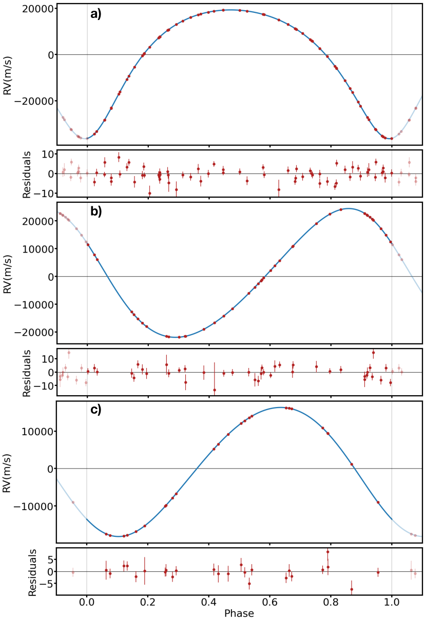
Figure 1: Best fit phased RV models for a) = J0310-31, b) = J1540-09, c) = J1928-38 with associated residuals. Doppler motion of the primaries seen here are caused by the secondary stars. Residuals have an RMS = $3.2$, $3.8$, and $3.0~{}\rm{m\,s^{-1}}$, respectively.

2) EBLM J1928-38 (J1928-38 for short). Its residual $\rm RMS~{}=~{}2.96~{}m\,s^{-1}$, better than J0310-31, close to its mean photon noise uncertainty $\rm\overline{\sigma_{RV}}~{}=~{}2.67~{}m\,s^{-1}$. Only $25$ measurements have been obtained on J1928-38 so far, which makes it more representative of the current state of the survey than J0310-31 is. These were collected between 2018-06-04 and 2019-09-14.

3) EBLM J1540-09 (henceforth J1540-09) has $\rm\overline{\sigma_{RV}}~{}=~{}3.86~{}m\,s^{-1}$, and $\rm RMS~{}=~{}3.75~{}m\,s^{-1}$, for 41 available spectra, observed from 2017-04-20 to 2020-03-06.

These targets were analysed using the kima RV analysis package (see next section). Their parameters can be found in Table 1. All data can be accessed in Tables 8 to Table 10. All measurements for these three systems are used, with no outliers found within those three datasets.

Table 1: Updated binary, system and derived parameters for the investigated binary systems. Uncertainties are given in the brackets, as the last two significant figures, except for $\sigma_{\rm jit}$ where uncertainties can be significantly asymmetric.

	EBLM J0310-31	EBLM J1540-09	EBLM J1928-38
System properties
TIC	89045042	32431480	469755925
TYC	7019-784-1	5600-377-1	7931-842-1
Gaia DR2	5057983496155992448	6317098582556256000	6739146911148825344
$\alpha$ [deg]1	03:10:22.62	15:40:08.99	19:28:58.85
$\delta$ [deg]1	-31:07:35.7	-09:29:02.2	-38:08:27.2
Vmag	9.33(02)2	10.865(38)3	11.20(12)2
Distance [pc]4	147.29(84)	206.0(1.8)	257.7(2.2)
$M_{\rm A}$ [$\rm M_{\odot}$]1	1.26(10)	1.18(10)	0.980(80)
Binary parameters
$P_{\rm bin}$ [day]	12.6427937(17)	26.338279(14)	23.322972(22)
$K_{\rm A}$ [$\rm{km\,s^{-1}}$]	27.87218(52)	23.17988(87)	17.26333(52)
$e_{\rm bin}$	0.308724(19)	0.120452(38)	0.073151(38)
$\omega_{\rm bin}$ [rad]	3.243410(80)	1.09802(37)	2.39117(75)
$T_{\rm peri}$ [BJD$-2,450,000$]	7934.64483(13)	7839.4468(15)	8258.5885(28)
System parameters
$\gamma$ [$\rm{km\,s^{-1}}$]	29116.0(10)	-55395.95(65)	16558.05(62)
$\sigma_{\rm jit}$ [$\rm m\,s^{-1}$]	2.77${}^{+0.45}_{-0.41}$	1.48${}^{+1.32}_{-1.45}$	0.089${}^{+1.153}_{-0.085}$
Derived parameters
$M_{\rm B}$ [$\rm M_{\odot}$]	0.408(20)	0.444(23)	0.268(14)
$a_{\rm bin}$ [$\rm AU$]	0.1260(31)	0.2037(53)	0.1720(44)
Notes: 1 - Martin et al. (2019), 2 - Høg et al. (2000), 3 - Munari et al. (2014), 4 - Gaia Collaboration (2018)

3 RV analysis with kima

For the analysis of the radial velocities and the calculation of detection limits, we use the kima package presented in Faria et al. (2018). The code models the RV timeseries with a sum of Keplerian functions from $N_{\rm p}$ orbiting planets, estimating the posterior distributions for all the orbital parameters.

To sample from the joint posterior distribution, kima uses the Diffusive Nested Sampling (DNS) algorithm from Brewer et al. (2011). Together with posterior samples, DNS provides an estimate for the marginal likelihood, or evidence, of the model, which can be used for model comparison (e.g. Brewer, 2014; Feroz et al., 2011). Fixing the values of $N_{\rm p}$ in sequence, we can use the ratio of the evidences to compare models with different number of planets. In addition, since DNS can be used in a trans-dimensional setting (Brewer & Donovan, 2015), the number of planets in the system $N_{\rm p}$ itself can be a free parameter in the analysis, and its posterior distribution can be estimated together with that of the orbital parameters. The posterior probability for each $N_{\rm p}$ value then allows for the same model comparison, with the advantage of being obtained from a single run of the algorithm.

The DNS algorithm samples from a mixture of distributions which is not directly the posterior. A total number of samples $N_{\rm s}$ from this target distribution results in a smaller number of effective samples $N_{\rm eff}$ from the posterior distribution. We obtain $N_{\rm eff}>20,000$ effective samples for each model, which is more than enough to accurately characterize the posterior.

Keplerian parameters are estimated from the effective posterior samples via the clustering algorithm HDBSCAN (McInnes et al., 2017). First, crossing orbits are removed from the posterior samples. Those are proposed Keplerian orbits that cross with each other, or those with an eccentricity which would cause their orbit to cross into the instability region of the binary and are therefore unphysical (e.g. Dvorak et al., 1989; Holman & Wiegert, 1999; Doolin & Blundell, 2011; Mardling, 2013). HDBSCAN is applied on the remaining posterior samples, highlighting dense regions in parameter space. The cluster corresponding to the Keplerian signal is plotted with the Corner package (Foreman-Mackey, 2016). Parameters are determined as the $50^{\rm th}$ percentile of the cluster, with $1\sigma$ uncertainties estimated from the $14^{\rm th}$ and $84^{\rm th}$ percentiles.

To decide between competing models that fit our data we use the Bayes factor. The Bayes factor (BF, here onwards) is the ratio of the Bayesian evidence of the two competing models, and provides a measure of the support in favour of one over the other (Robert E. Kass; Adrian E. Raftery, 1995; Trotta, 2008). Table 2 adapted from Trotta (2008) shows how the BF is measured and introduces the Jeffreys’ scale (Jeffreys, 1961) as a measure of evidence strength.

Table 2: Table of Bayes Factors (BF) along with corresponding probability, sigma values (standard deviations away from the mean of a normal distribution), and the “Jeffreys’ scale” adapted from Trotta (2008).

BF	Probability	sigma	Evidence strength
$\lesssim 3$	$<0.750$	$\lesssim 2.1$	Inconclusive
$3$	$0.750$	$2.1$	Weak
$12$	$0.923$	$2.7$	Moderate
$150$	$0.993$	$3.6$	Strong

To guide our identification of planetary candidates we follow the same Jeffreys’ scale, but use custom thresholds that affect what response we have to the system. Like Trotta (2008), we use $\rm BF=12$ as a threshold for ’moderate’ evidence. To identify planetary candidates worthy of additional follow-up (to apply for additional telescope time for instance), we use $\rm BF>6$. Regularly, $3\sigma$ marks a detection in Astronomy. To make sure we are over that value, we place a threshold at $\rm BF=35$. Any system reaching that level continues to be observed as any other, but we analyse its data more regularly than once a year. To visually track increasing evidence for a planetary signal, we place an additional division at $\rm BF=70$. Finally we place our upper threshold $\rm BF=140$, after which observations cease to be blind and we start to target specific epochs that represent poorly sampled orbital phases, or alternate solutions (eccentricity, $2\times P_{\rm p}$, etc). We use the thresholds described here in our insertion/recovery exercise below.

Contrary to a regular planetary system, a circumbinary SB1 system is dominated by the reflex motion caused by the secondary star (typically tens of $\rm km\,s^{-1}$) and extremely well constrained by the data. In addition, we know there cannot be a planet at an orbital period $\lesssim 4~{}P_{\rm bin}$ due to the instability region (Dvorak et al., 1989; Holman & Wiegert, 1999; Doolin & Blundell, 2011; Mardling, 2013). In contrast, we have no idea whether a planet is within the system, or what its parameters might be. By default kima applies a common prior for all the orbiting objects (secondary, or planet) in a given model, which is not well adapted to our case. Particularly, there is no doubt that there is a secondary star in the system, and as such no need for the nested sampler to test that hypothesis.

In this context, kima can instead use the so-called known object mode, where a specific set of priors can be placed on the binary properties, and another set of priors is used to explore the presence/parameters of putative planets. At each step kima then fits for the binary (the known object) and any additional Keplerian signal present in the data. Using this mode, the nested sampler only computes evidence for $\geq 1$ Keplerian function, therefore only testing for the presence of circumbinary planets ($\geq 0$ planets).

A typical kima run with $200,000$ saves, resulting in $N_{\rm eff}\approx 25,000-35,000$ posterior samples (depending on data-set) takes $\approx 180$ minutes on a standard laptop computer.

4 Methods & Simulations

Here, we describe our methods, which are used similarly on all the systems we monitor in the survey. First, we give a simple parameterisation of the model. Then, we detail and justify the priors we use within kima (see also Table 3). We then demonstrate using kima to produce robust and fully Bayesian detection limits. Following that, we perform a more traditional insertion-recovery test of static Keplerian signals to compare with our kima detection limits. We then test the validity of injecting static Keplerian signals in comparison to N-body simulations. Finally, we discuss how our process compares with previous methods for detection limits, both for single and binary stars.

4.1 Model setup

With kima we assume independent, static Keplerian orbits for the binary and any circumbinary planets. This neglects the fact that the orbits of the planet and binary will evolve through three-body interactions (e.g. Martin & Triaud 2014; Kostov et al. 2014). Martin et al. (2019) however found such interactions to be negligible with respect to the CORALIE BEBOP survey. We will briefly verify if this assumption still holds with our more precise HARPS data in Sect. 4.4, where we test the injection and retrieval of N-body simulated RV signals.

The Keplerian models we fit to the data are defined by the following parameters. For the binary we have $P_{\rm bin}$ (the orbital period), $K_{\rm A}$ (the semi-amplitude of the primary star, caused by the secondary), $e_{\rm bin}$ (the binary’s orbital eccentricity), $\omega_{\rm bin}$ (the argument of periastron) and $\phi_{\rm bin}$ (the starting phase of the orbit). We can calculate the time of periastron passage from these parameters using ${T_{\rm peri}}=t_{0}-(P\times\phi)/(2\pi)$, where $t_{0}$ is the chosen epoch. The number of planets in the system is referred to as $N_{\rm p}$. Planetary parameters are defined like for the binary, but written with a subscript p, e.g. $P_{\rm p}$ for a planet’s orbital period.

In addition, we fit for the systemic velocity $\gamma$, and for a jitter term, $\sigma_{\rm jit}$ that rescales the uncertainties on the data. An increase in this parameter is penalised when computing the likelihood. We can also fit for offsets in data between instruments, but this not necessary for the three systems we analyse here.

4.2 Prior distributions

We use priors similar to those laid out in Faria et al. (2020), but adapted to circumbinary planets. As described in Sect. 3, we treat the signal produced by the secondary star as a known object, taken to be obviously present in the data and place tight priors on its parameters. We only compute Bayesian evidence for any additional signals to the inner binary. This is an advantage of using kima, both the orbit of the binary and any additional signal are fit to the data simultaneously, each posterior sample obtained has a corresponding binary fit. Table 3 shows the prior distributions utilised in our analysis.

The secondary’s orbital parameters prior distributions are based on values from an initial fit. We take the mode of each binary parameter and set to the prior to uniformly explore a range around that value. That range is determined from fitting all of the binaries in our sample. For instance, we explore $\pm 0.01~{}\rm day$ around the orbital period, and $\pm 10~{}\rm m\,s^{-1}$ around the semi-amplitude (Table 3). While these might seem tight, the typical precision obtained on $P_{\rm bin}$ and $K_{\rm A}$ is $100\times$ less than the prior ranges we set (see Table 1). As such the binary priors we chose are wide enough to enclose the true parameters and their uncertainties.

To search for additional signals besides the binary (i.e. circumbinary planets), we use a uniform distribution for $\gamma$, $\phi$, $\omega$, and $N_{\rm p}$, as there is no reason to favour any particular value within these parameter spaces.

For planetary eccentricities, we utilise a Kumaraswamy distribution (Kumaraswamy, 1980), using values for our shape parameters as $\alpha=0.867$ and $\beta=3.03$ as justified in Kipping (2013), closely resembling the Beta distribution described there. A Kumaraswamy distribution favours lower values but still permits the exploration of higher eccentricities when the data allows.

The most sensitive parameter to sample when determining robust detection limits is planetary semi-amplitudes $K_{\rm p}$. For this reason, we use a transformed Log-Uniform (Jeffreys) prior. We cap the upper range, choosing $100~{}\rm m\,s^{-1}$ (any signal greater than this would be obvious in our data). Thanks to various tests, we noticed that setting a specific lower limit to $K_{\rm p}$ influenced our ability to recover planets and estimate robust detection limits. When we set the lower limit too high (e.g. $1~{}\rm{m\,s^{-1}}$) it excludes any signals $<1~{}\rm{m\,s^{-1}}$ in strength that could lie formally undetected in our data, but effectively ignoring any contribution they may have on other signals and parameters. If instead we set the limit too low (e.g. $0.01~{}\rm{m\,s^{-1}}$), the sampler does not explore the higher $K_{\rm p}$ sufficiently (since they become relatively less likely). This can bias the detection limit to lower $K_{\rm p}$ due to low number statistics in the posterior, producing over-confident detection limits.

Instead of setting a lower value we insert a knee, to give less priority to signals below a set value. Gregory (2005) advises using a knee at $1~{}\rm{m\,s^{-1}}$, which was $1/10$ of their typical RV uncertainty. As our survey utilises RV data from both SOPHIE, HARPS and ESPRESSO, our uncertainties approach $1~{}\rm{m\,s^{-1}}$, we set our knee to $0.1~{}\rm{m\,s^{-1}}$. For values of $0~{}<~{}K_{\rm p}<0.1~{}\rm{m\,s^{-1}}$ the distribution acts as a uniform prior, whereas for $K_{\rm p}\geq 0.1~{}\rm{m\,s^{-1}}$ the priors follow the usual Jeffreys prior (see Gregory, 2005).

For all other parameters we employ Log-Uniform (Jeffreys) priors since the range of values can span several orders of magnitudes. This goes for $\sigma_{\rm jit}$ and $P_{\rm p}$.

The lower limit for the $P_{\rm p}$ prior is set to $4\times P_{\rm bin}$, following the instability region (see Sect. 3). This is a slightly conservative estimate for the instability region. For completeness, we explored the effect of placing a lower limit at $P_{\rm p}<P_{\rm bin}$. Results were similar, with the only effect being that posterior samples were dispersed over a larger parameter space resulting in a coarser posterior.

We place the upper limit at $P_{\rm p}=$1\text{\times}{10}^{3}$~{}\rm{day}$, roughly the time-span of our longest observed systems: J0310-31. For simplicity and to allow for a fair comparison, this limit is used for all three systems. We increase the maximum limit to $$2\text{\times}{10}^{4}$~{}\rm{day}$ to generate detection limits, as described in Sect. 4.3, and witness how the detectable semi-amplitude increases with increasing orbital period after exceeding the time-span of the data. When seeking planetary candidates, we prefer using a maximum period of $$1\text{\times}{10}^{3}$~{}\rm{day}$, which saves computational power and ensures a finer sampling of the posterior. The presence of a planetary signal with $P_{\rm p}>$1\text{\times}{10}^{3}$~{}\rm{day}$ in our data would be identifiable as an over-density of posterior samples at the upper limit of this prior. In which case we adjust this limit as required. The limit on $P_{\rm p}$ will extended as we accumulate more data.

Table 3: Prior distributions used in RV model for binary and planetary signals in kima

Parameter	Unit	Prior distribution
		Binary	Planet
$N_{\rm p}$		$1$	$\pazocal{U}(0,3)$ or $1$
$P$	days	$\pazocal{U}(P_{\rm bin}\pm{0.01})$	$\pazocal{LU}(4\times P_{\rm bin},$1\text{\times}{10}^{3}$$ or $${10}^{4}$)$
$K$	$\rm{m\,s^{-1}}$	$\pazocal{U}(K_{\rm A}\pm{10})$	$\pazocal{MLU}(0.1,100)$
$e$		$\pazocal{U}(e_{\rm bin}\pm{0.0005})$	$\pazocal{K}(0.867,3.03)$
$\phi$		$\pazocal{U}(0,2\pi)$
$\omega$		$\pazocal{U}(0,2\pi)$
$\sigma_{\rm jit}$	$\rm{m\,s^{-1}}$	$\pazocal{LU}(0.001,10\times\rm{rms})$
$\gamma$	$\rm{m\,s^{-1}}$	$\pazocal{U}(V_{sys}\pm{100})$

• Notes: $N_{\rm p}$ denotes the Number of Planetary Keplerian signals to fit to the data. $P_{\rm bin}$ and $e_{\rm bin}$ denote the Period and eccentricity of the binary respectively. $K_{\rm A}$ denotes the semi-amplitude of the primary star, caused by the secondary. $\pazocal{U}$ denotes a uniform prior with an upper and lower limit, $\pazocal{LU}$ is a log-uniform (Jeffreys) prior with upper and lower limits, $\pazocal{MLU}$ is a modified log-uniform prior with a knee and upper limit, and $\pazocal{K}$ is a Kumaraswamy prior (Kumaraswamy, 1980) which takes two shape parameters.

4.3 Detection limit method

A unique feature of a diffusive nested sampler such as kima is that when forced to explore higher $N_{\rm p}$ than is formally detected, the sampler will produce a map of all signals that are compatible with the data. Since those proposed signals remain formally undetected, the posterior naturally produces a detection threshold. In our case this is made simpler by kima’s known object mode (see Sect. 3), and the fact that no planets have been detected in those three systems thus far. We describe in Sect. 5.3 how we calculate a detection limit when a planetary signal is already present in the data.

Later, we compare our results to a more traditional insertion-recovery test, the method of choice to assess detectability and measure occurrence rates in radial-velocities surveys (Cumming et al., 2008; Konacki et al., 2009; Bonfils et al., 2013; Martin et al., 2019; Rosenthal et al., 2021; Sabotta et al., 2021).

Using a diffusive nested sampler like kima also provides immediate advantages over insertion-recovery test. kima samples all orbital parameters in a fine manner. Particularly, this means that all orbital phases, all eccentricities and all periastra are sampled when typically only a small number of phases are tested, and that eccentricities are nearly always forced to zero. Detection limits obtained with kima marginalise over more orbital parameters than is computationally feasible with insertion-recovery tests, and kima assumes Keplerian signals, rather than sinusoidals (see next section).

To create a detection limit, we run kima with priors as in Table 3 except that we fix $N_{\rm p}=1$. kima marginalises over all allowed parameter space, searching for any possible Keplerian signals producing a reasonable likelihood, in the process ruling out Keplerians that would otherwise have been detected.

A key to producing a robust detection limit is to produce a well sampled posterior. For each system we compute three runs, ensuring $>20,000$ samples are obtained in each. To gather consistent results we set the number of saves in kima to $200,000$. The resulting ($K_{\rm p},P_{\rm p}$) posterior’s density is plotted in Figures 2 and 3 as a greyscale hexbin, with the detection limit being the top envelope.

To compute the detection limit, we separate the posterior in log-spaced bins in $P_{\rm p}$, and within each bin we evaluate the maximum $99^{\rm th}$ percentile of the $K_{\rm p}$ distribution. This is done with the caveat that $\geq 2$ posterior samples must lie above the chosen sample in a given bin. We do this to prevent the detection limit from being affected by small number statistics in individual bins. We calculate a detection limit for each of the three runs we perform on each system, which we show with faded blue lines in Figures 2 and 3. We also draw the detection limit obtained when combining all posterior samples from the three runs into a single sample, with a solid blue line. Proceeding this way allows us to produce a mean detection limit and to obtain a visual estimate of the uncertainty of that limit for each bin. Overall, all runs are compatible with one another. We stop computing the detection limit for all $P_{\rm p}$ exceeding the first $P_{\rm p}$ bin where the number of samples in the top $10\%$ of $K_{\rm p}$ prior is larger than three, which is where the posterior is affected by the upper limit set for the $P_{\rm p}$ prior.

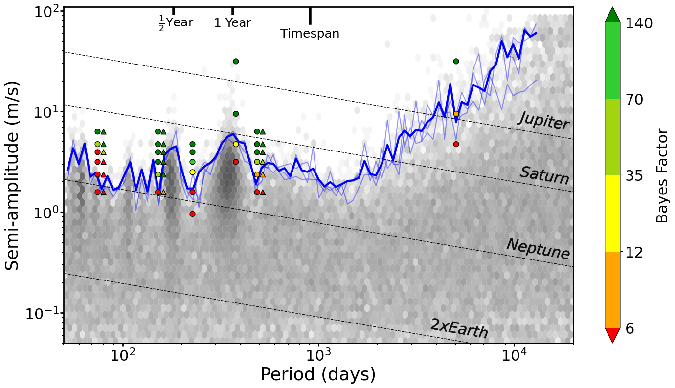
Figure 2: Hexbin plot denoting the density of posterior samples obtained from three separate kima runs on J0310-31 with $N_{\rm p}$ fixed $=1$, as a grayscale. Faded blue lines show detection limits calculated from each individual run on the system as described in the text. The solid blue line shows the detection limit calculated from all posterior samples combined. Coloured symbols indicate the Bayes factor results of injection/recovery tests and correspond to the colour bar on the right. Circles are for injected static Keplerian sinusoidal signals, whereas triangles are for N-body simulated injected signals. The Keplerian and N-body signals are injected at the same orbital periods but are represented slightly offset horizontally here for visual clarity. The faded red dashed lines show masses of solar system planets for comparison.

4.4 Injection and Recovery Tests

The seminal (single-star) radial-velocity surveys of Cumming et al. (2008); Mayor et al. (2011); Howard et al. (2010) used injection and recovery methods as a means of determining injection limits. First, all known planets are removed from the data. Then a sinusoid of varying amplitude, period and phase is used to model a putative exoplanet, and applied to the data. Following, that, a periodogram of the data (typically a Generalised Lomb-Scargle) is computed. If it produces a peak below a certain false alarm probability (typically $<1\%$) near the injected period, the simulated planet is considered “detected”. By reproducing this procedure over a grid of $P_{\rm p}$ and $K_{\rm p}$ inserted signal, it is possible find out for which values the planet is no-longer detectable. Martin et al. (2019) followed this approach for the CORALIE BEBOP survey, with one key difference that the planet signal was injected to a radial velocity data set where the binary signal had already been removed.

Whilst this traditional approach may appear similar to ours, in practice they are distinct. When we use our Bayesian approach with kima to produce detection limits we answer the question "what is compatible with the data?", whereas with an insertion-recovery test, we ascertain "can this specific signal be found?".

Here we create injection-retrieval tests for our three targets. There are two purposes of this. First, we investigate compatibility between our Bayesian kima-derived limit and the more traditional approach of injecting static Keplerian signals. Second, we follow the approach of Martin et al. (2019) to inject not just static sinusoids but an N-body derived signal using rebound, including all dynamical interactions between the planet and binary, to test the validity of the previous step.

We add one circumbinary planet signal to the original data, and do so for a number of planetary semi-amplitudes $K_{\rm p}$ and orbital periods $P_{\rm p}$. kima is then used to recover any Keplerian signals in the modified data-set with the resulting Bayes factors providing a measure of signal recovery success.

The choice of $K_{\rm p}$ and $P_{\rm p}$ at which we inject simulated signals is informed by the data itself. For $K_{\rm p}$, values are chosen as multiples of the residual RMS of each system. Values used can be found for each system in Tables 4-7.

For $P_{\rm p}$ there are three periods we test for all three targets. The first is $5.9\times P_{\rm bin}$, which is similar to known circumbinary systems (Martin, 2018) and slightly offset from the often unstable 6:1 mean motion resonance (Quarles et al., 2018). We also test $12\times P_{\rm bin}$ and $486~{}\rm{days}$ ($365\times 4/3$, to avoid but be close to the $1~{}\rm yr$ alias). In some cases, we also simulate specific orbital periods, coinciding with features of the detection limits described in Sect. 4.3.

Each inserted signal has an eccentricity $e_{\rm p}=0.01$ (small but non-zero), and argument of periastron $\omega_{\rm p}=0$.

Then, we run kima as described previously, using priors as in Table 3, including a uniform prior on $N_{\rm p}=U(0,3)$, reproducing how we conduct an open search of the system. Bayes factors are computed from each run and results are plotted in Figures 2 and 3 as coloured points. Their values can also be found in Tables 4 to 7.

The binary and putative circumbinary planets for the three chosen periods are then simulated for the J0310-31 system using the rebound N-body code (Rein & Liu, 2012), with the IAS15 integrator (Everhart, 1985; Rein & Spiegel, 2015). First we remove the best fit binary model from J0310-31’s observed radial-velocity measurements, producing residuals. Then we use rebound to simulate a radial-velocity model of the binary and putative planet at each epoch of observation. We add this model to the residuals. Doing this preserves the scatter, uncertainties and observational cadence obtained in reality. kima is ran once again on each N-body simulated dataset, and Bayes factors computed and compared to those resulting from the injected static Keplerian signals.We discuss the result of this test in Sect. 5.3. All Bayes factor values are plotted in Fig.  2 as coloured triangles offset to the right, and can also be found in table 5.

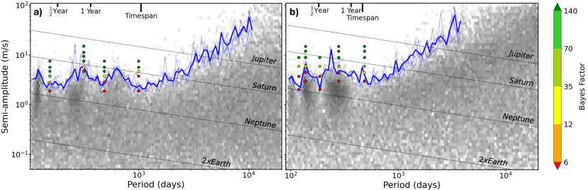
Figure 3: Same as in figure 2 but for three separate kima runs on J1540-09 (a), and J1928-38 (b) with $N_{\rm p}$ fixed $=1$. All injected signals here are static Keplerian sinusoidal.

5 Results and Discussion

We begin by providing updated parameters on the three binary systems investigated. Then, we discuss the calculated detection limits for each binary system, along with how they compare to our Keplerian injection and recovery tests. Following this we discuss and present our results from the comparison between Keplerian and N-body simulation injection and recovery. We discuss how nested sampling provides more robust detection limits. Particularly, we describe how traditional insertion-recovery exercises over-estimate their ability to retrieve planets by assuming zero eccentricity.

5.1 Updated Binary Parameters

Table 1 shows updated orbital parameters from our most recent data for the systems investigated in this work. We provide $1\sigma$ uncertainties for each parameter, in parenthesis. Uncertainties are symmetric and varying only in the second significant figure, where the largest of the two values were taken. $\sigma_{\rm jit}$ is the only parameter that demonstrated an asymmetric distribution (tending to zero), where we consequently provide asymmetric uncertainties. Values agree with Martin et al. (2019) to within $1-2\sigma$ for all parameters other than $\omega_{\rm bin}$ and correspondingly $T_{\rm peri}$. Improvements in parameter precision of around $70\%$ are be attributed to the increased number of high-precision measurements acquired using the HARPS spectrograph.

5.2 Detection limit results

Figures 2 and 3 show the results of our detection limit analysis for EBLM J0310-31, J1540-09, and J1928-39 respectively. The greyscale hexbins show the density of posterior samples from all kima runs on the targets. The faded blue lines are the calculated detection limit from three individual run containing $200,000$ saves, and $>20,000$ posterior samples. The solid blue line is calculated from all posterior samples combined. Coloured dots represent the results for each individual injection and recovery test as outlined in Sect. 4.4. The colour of these points represent the Bayes Factor (BF) discussed in Sect. 3, and measure the probability of recovery for the injected Keplerian signals. Every sample in the posterior used to compute detection limits involves a free fit of the binary as a well as a proposed planetary signal, producing a detection limit that marginalises over the binary parameters, an essential element for BEBOP.

From these plots, it is evident that different runs of kima produce consistent detection limits with one another. The only inconsistencies are due to a low number of samples within a particular bin, a situation easily resolved by increasing the number of saved posterior samples. We also note that the posterior below the limit is uniformly sampled across parameter space, an indication of the reliability of the method we followed.

The detection limit plots also show many features that are regularly seen in detection limits for exoplanets using the radial-velocity method. For all three systems we see an increased density of posterior samples, and a consequently raised detection limit near $0.5$ and $1~{}\rm yr$ orbital periods, corresponding to yearly aliases, caused by seasonal gaps in observations. In addition, we observe that our detection capability is broadly horizontal for $P_{\rm p}$ below the timespan of our data. Then, it increases linearly in log until it hits the upper limit of the $P_{\rm p}$ prior. For J0310-31, we reach a mean $K{\rm p}$ detection of $1.49~{}\rm m\,s^{-1}$, for J1540-09, we get $2.06~{}\rm m\,s^{-1}$, and $2.15~{}\rm m\,s^{-1}$ for J1928-38. For these three systems, we outperform any produced by the TATOOINE survey (Konacki et al., 2010) despite our systems being fainter by an average four magnitudes, validating our choice to monitor single-lined binaries to seek circumbinary exoplanets. These detection limits can be translated into masses, which are shown by additional lines in Figures 2 and 3. Typically, we are sensitive to planets with masses between Neptune’s and Saturn’s for orbital periods between 50 to 1000 days respectively, a milestone.

Injection-recovery test results are consistent with the detection limits obtained with kima at almost all orbital periods tested on each system. The largest deviation can be seen in Fig. 2 for J0310-31 at $74.59~{}\rm{d}$. Where the detection limit is approximately $2~{}\rm{m\,s^{-1}}$ lower than the recovered injected signal strength. This is the only location where such a deviation is observed.

Figure 4 is an example of how the value of the Bayes Factor evolves with the number of posterior samples during a kima run. Our example is J0310-31 data, with an injected planetary signal with $P_{\rm p}=227.57~{}\rm{d}$, and $K_{\rm p}=3.16~{}\rm{m\,s^{-1}}$. The uncertainty on the Bayes Factor (blue area) is estimated assuming a multinomial distribution. We use this figure as an indicator for fit convergence, i.e once the line asymptotes on a BF value the fit has converged.

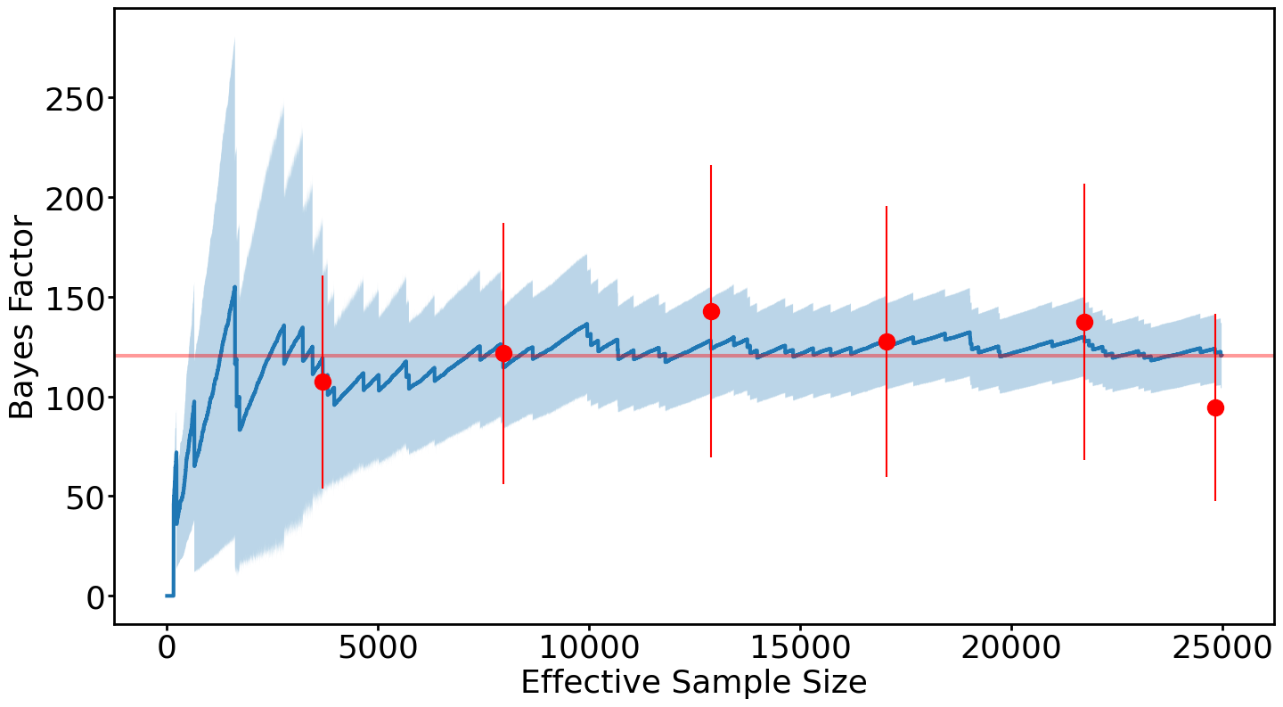
Figure 4: Plot of Bayes Factor (BF) vs number of posterior samples from a kima run with a $227.57~{}\rm{d}$, $3.16~{}\rm{m\,s^{-1}}$ injected signal in J0310-31. In blue, we show the cumulative Bayes factor as a function of the number of posterior samples. The blue line shows the BF values, and and their running uncertainty are drawn as the shaded blue region. We add one red dot after $10$ $N_{\rm p}=0$ samples to show the BF value then, with their uncertainties. The horizontal red line shows the final BF value calculated with all posterior samples.

We also check how often we recover the Keplerian signal we insert. We find that orbital parameters of injected signals detected with $\rm BF>35$ are typically recovered to within $3\sigma$ or $10\%$ of their original values, except those with periods close to one or half a year. This is true for injected Keplerian signals, as well as the rebound injected signals.

The chosen phase of the injected Keplerian signal could in principle cause the discrepancy between the methods seen at $P_{\rm p}=74.59~{}\rm day$ for J0310-31. Figure 5 shows the same posterior samples as those in Fig. 2 but split into five different phase bins, with a detection limit calculated for each. Doing this is simple with kima, we simply select all posterior sample within a specific phase bin and reproduce the method in Sect 4.3. As can be seen in the figure, varying phase has little effect on the detection limit, which is the case for each target investigated. This consistency seen between phase bins further demonstrates how robust and consistent our detection limits are. This also highlights the usefulness and importance of using nested samplers such as kima to compute detectability curves.

Figure 5: Hexbin plot of posterior samples for J0310-31 as in figure 2. The coloured lines here indicate the detection limits calculated with the posterior samples split into five even phase bins with the black line representing the phase bin containing $\phi=0$.

5.3 Rebound Simulation Results Comparison

Results from systems simulated using rebound are shown in Fig. 2, as coloured triangles offset to the right from similar, but Keplerian-only simulations. The only evident deviation between the two simulations occurs at the shortest period investigated ($74.59~{}\rm{day}$) here the Bayes factor for the rebound simulated data is higher for $K_{\rm p}=3.95~{}\rm{m\,s^{-1}}$.

The agreement in those results (see Table 5) confirms that assuming Keplerian functions has no obvious detriment to circumbinary planet detection within our current data just like for any planetary system so far, and as we had already seen in Martin et al. (2019) with more imprecise CORALIE data. This simply means that assuming a static Keplerian signal is sufficient for discovery. However, dynamical fits are known to be useful to constrain the physical and orbital parameters of circumstellar planetary systems (e.g. GJ 876; Correia et al., 2010), and would likely be the case for circumbinary systems, as they have been for HD 202206 (Correia et al., 2005; Couetdic et al., 2010), a system comparable to a circumbinary configuration.

To better understand the non-Keplerian signal, we visualise the amplitude of the Newtonian interactions in Fig. 6. We use rebound to simulate nightly RV data, for $K_{\rm p}=6.32~{}\rm m\,s^{-1}$ at $P_{\rm p}=74.59~{}\rm days$ (the shortest period and highest mass planetary signal simulated in this work, producing the largest Newtonian perturbation), over the timespan of our data on J0310-31. Figure 6 depicts the residuals after fitting and removing the Keplerian binary and planetary signals from the N-body simulated dataset. The residuals show that N-body model diverges from the Keplerian model due to apsidal precession ($\dot{\omega}_{\rm bin}$). However, for the timespan of our current data that divergence remains comparable to the residuals’ RMS. Assuming Newtonian effects are non-negligible will likely cease to be valid for longer time-series.

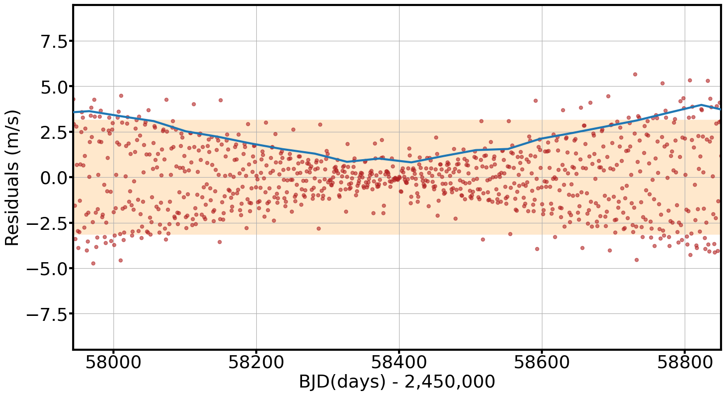
Figure 6: Plot of residual radial velocity amplitude as a function of time, after removing a Keplerian binary signal from N-body simulated J0310-31 radial-velocity dataset. Simulated data are computed with rebound including the binary and an orbiting circumbinary planet with $P_{\rm p}=74.59~{}\rm{d}$ and $K_{\rm p}=6.32~{}\rm{m\,s^{-1}}$. To reveal the Newtonian perturbation, we plot one point for each night over the entire duration of our dataset. The blue line depicts $1.3\times$ RMS within bins $45~{}\rm day$ wide. We use this line as a visual guide to the amplitude of the effect. The shaded orange region illustrates the RMS scatter obtained on the data we collected on J0310-31. The bow-tie shape of the residuals is caused by apsidal motion of the binary ($\dot{\omega}_{\rm bin}$), caused by the planet, which a Keplerian model does not include.

5.4 Post-Newtonian Effects

Radial velocity measurements of binary stars are also affected by weaker effects, such as tidal distortion, gravitational redshift, transverse Doppler and light time travel effects (Zucker & Alexander, 2007; Konacki et al., 2010; Arras et al., 2012; Sybilski et al., 2013). kima assumes purely Keplerian functions, ignoring these effects, here we explore what impact this may have on our fit, and particularly on our ability to retrieve planets.

We calculate the magnitude of tidal distortion on our RV measurements as in Arras et al. (2012), and find their amplitude is $<0.7~{}\rm m\,s^{-1}$ for the three systems we investigate in this paper, an insignificant contribution to the observed RV scatter. We do note however, that for the shortest period binaries in the BEBOP survey, the magnitude of this effect becomes significant (with respect to the RMS of the systems) and should be accounted for in any further analysis.

Computing equations from Zucker & Alexander (2007) for the parameters of each of our three systems, we find the magnitude of transverse Doppler effects to be $<2.2~{}\rm m\,s^{-1}$, and the peak to peak variation $<1.6~{}\rm m\,s^{-1}$. Similarly, we find the magnitude and peak to peak variation of light time travel effects is $<2.7~{}\rm m\,s^{-1}$. The only relativistic effect found to be greater than the RMS on these systems is that of gravitational redshift, with a maximum amplitude of $13.9~{}\rm m\,s^{-1}$ but a peak to peak variation of $<6.5~{}\rm m\,s^{-1}$.

To better asses the impact of these effects on our work, we simulate a purely Keplerian binary signal for J0310-31 using the same cadence as our observations were obtained in, and add these post-Newtonian effects. We then fit the data using kima. Figure 7a shows residuals after removing the best fit Keplerian model of the binary. The residuals have an amplitude of $\approx 0.1~{}\rm m\,s^{-1}$ and a signal phasing with the binary (as expected). This shows that most of the post-Newtonian effects are absorbed by the Keplerian fit.

We now use kima once more, to "search for a planet" in these residuals, in order to study how the algorithm behaves in the presence of additional coherent signals. The posterior of that fit is plotted in figure 7b, and demonstrates the periodicity of these remaining signals at harmonic periods of the binary with low semi-amplitude.

Individually these effects boast significant amplitudes, but as their functional forms resemble, and phase, with a Keplerian, only small differences are produced: Our simulations show that the majority of the post-Newtonian signals are absorbed into our fit. They are absorbed primarily into the systemic velocity, and lead to a small underestimation of the secondary’s semi-amplitude. For J0310-31, ignoring post-Newtonian effects in this experiment creates an underestimated $K_{\rm A}\approx 4~{}\rm m\,s^{-1}$, corresponding to a $0.01\%$ deviation. We conclude that these effects do not affect the detection limits of this paper greatly, and can be safely ignored for our purposes.

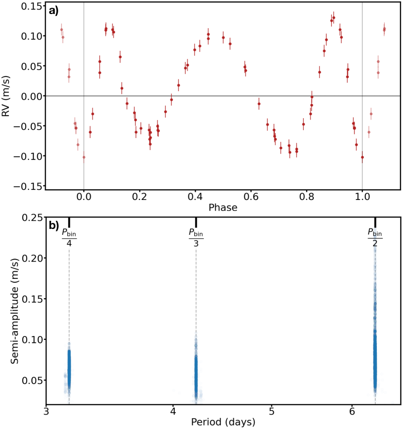
Figure 7: a) Phased RV residuals from the best fit model of J0310-31 simulated binary and additional post-Newtonian effects only. Residuals have an RMS $=~{}0.07~{}\rm m\,s^{-1}$. b) Semi-amplitude vs period plot of posterior samples from a kima run on the residuals seen in plot a). Posterior samples are located at half, third and a quarter of J0310-31’s binary orbital period.

5.5 Detection limits in the presence of planetary signals

Detection limits thus far are all generated from our current data on systems purposefully chosen with no candidate planetary signals. The ultimate goal of the BEBOP survey is to detect RV signals of circumbinary planets in our data. Once a system is found to have a planetary signal, a detection limit is required to rule out the presence of additional companions above our calculated mass limit. To this end, we calculate the detection limit for J0310-31 with our N-body simulated data-set containing an injected $4.74\rm m\,s^{-1}$, $486$ d signal. A signal of this strength is easily detected in the data (see Tab. 5 for its Bayes factor value). We identify the injected signal as in Sect. 4.4, with $N_{\rm p}$ varying uniformly from $0$ to $3$, as is standard for the survey. Figure 8 shows the resulting posterior samples, along with a green dot illustrating the semi-amplitude and orbital period of the injected signal. To obtain a recovered detection limit we subtract the Keplerian signal corresponding to the posterior model with the highest likelihood from the simulated data. Once subtracted, we run kima again as in Sect. 4.3 and calculate the red recovered detection limit from the resulting posterior samples. The blue line seen in Fig. 8 is taken from Fig. 2 for reference, and the recovered red line closely resembles the original blue detection limit. We note that while this approach is not strictly Bayesian, it recovers the correct detection limit, and is expected to affect only a few systems (with planets) within the survey.

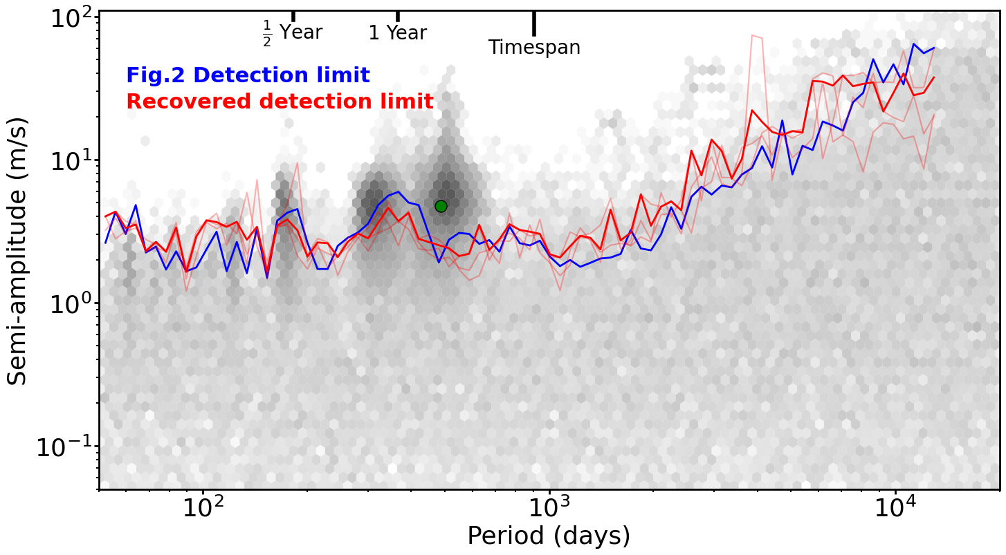
Figure 8: Hexbin plot of posterior samples obtained from three separate kima runs on J0310-31 with an additional $486$d signal located at the green point, with $N_{\rm p}$ free between $0$ and $3$. The blue line shows the detection limit as seen in Fig. 2. Faded red lines show detection limits calculated from each individual run on the system after having removed the most likely $N=1$ signal from the data. The solid red combines all these posterior samples together.

5.6 The Dangers of Assuming Circular Orbits

Thanks to our use of kima to produce detection limits we are able to explore the effect of assuming $e_{\rm p}=0$ on detection limits for exoplanet radial-velocity surveys.

Most often detection limits are produced with multiple insertion-recovery tests. To increase efficiency, and remain computationally tractable, a number of assumptions are made. Circular orbits are generally assumed in the inserted signals used to calculate detection limits because this removes two dimensions: $e_{\rm p}$ and $\omega_{\rm p}$ (e.g. Cumming et al., 2008; Zechmeister et al., 2009; Howard et al., 2010; Bonfils et al., 2011; Mayor et al., 2011; Bonfils et al., 2013; Martin et al., 2019; Sabotta et al., 2021). In addition, a short number of discrete planet phases $\phi_{\rm p}$ are usually sampled (e.g. 10; Martin et al. 2019 or 12; Zechmeister et al. 2009; Bonfils et al. 2011, 2013).

Commonly when orbits are assumed circular, investigators invoke Endl et al. (2002) as a justification. Endl et al. (2002) investigated the effect of eccentricity on their detection limit for HR 4979, using insertion and recovery. They test five planetary orbital periods $P_{\rm p}$, each with one corresponding semi-amplitude $K_{\rm p}$, and vary $e_{\rm p}$ over $9$ values and $\omega_{\rm p}$ over $4$, creating 180 $(P_{\rm p},K_{\rm p},e_{\rm p},\omega_{\rm p})$ signals. They only test one phase angle $\phi_{\rm p}$. At the time, producing these simulations represented a significant computational effort, however nowadays this appears as a rather coarse grid. From this exercise, Endl et al. (2002) conclude that eccentricity can affect detection limit calculations, but find that their detection limits assuming $e_{\rm p}=0$ are valid for $P_{\rm p}\gtrapprox 365~{}\rm days$, so long as the simulated Keplerian has $e_{\rm p}\lesssim 0.5$. More recently Cumming & Dragomir (2010) also concluded that assuming circular orbits provides a good agreement with upper semi-amplitude limits for $e_{\rm p}\lesssim 0.5$ when recovering signals with a periodogram. These particular results have been invoked to justify the assumption of circular orbits ever since.

Interestingly, for $P_{\rm p}\leq 365~{}\rm days$ (Endl et al., 2002) find their detection limit is only valid if the inserted signal has $e<0.3$. However this recommendation has not been followed, and assuming circular orbits for short period is prevalent throughout the literature. From our analysis, we can show how eccentricity affects the detection limit over the entire period range. Our kima runs contain $>70,000$ posterior samples that naturally explore all orbital parameters.

Figure 9 shows the same detection limit for EBLM J0310-31, as calculated before, in blue using all posterior samples. Alongside we plot a red detection limit produced in exactly the same way, except using only samples with $e_{\rm p}<0.1$, and green with $e_{\rm p}<0.5$ (the limit stated by Endl et al., 2002; Cumming & Dragomir, 2010). For the three systems explored in this work, the red detection limit is systematically lower, by an average of $24.7\%$ or $\sim 1~{}\rm m\,s^{-1}$ for periods $<1000~{}\rm day$. The green detection limit is also systematically lower by an average of $13.3\%$ or $\sim 0.6~{}\rm m\,s^{-1}$ for the same periods. Figure 10 demonstrates how the two lower detection limits differ from the original for J0310-31 with period. We note an increase in divergence from the original detection limit at $P_{\rm p}$ exceeding the timespan of the data ($>1000~{}\rm day$ here), to a maximum of $39.9\%$ at $\sim 4000~{}\rm days$. This maximum difference corresponds to $3.5~{}\rm m\,s^{-1}$ ($\sim 120~{}\rm M_{\oplus}$)! Our results are consistent with Wittenmyer et al. (2006) who are able to exclude planets with masses $\gtrsim 2~{}\rm M_{Jup}$ by assuming $e_{\rm p}=0$, and masses $\gtrsim 4~{}\rm M_{Jup}$ if instead they assume $e_{\rm p}=0.6$ at a given $P_{\rm p}\sim 4300\rm~{}days$, a $50\%$ difference, comparable to our $40\%$.

Here we remind the reader that we assume a Kumaraswamy distribution as our prior on $e_{\rm p}$, which already favours low $e_{\rm p}$, as is seen in observations (Kipping, 2013). Even though circumbinary planets discovered thus far are known to have relatively low eccentricities ($e<0.15$ Martin, 2018), we strongly caution against assuming circular orbits when calculating detection limits in any survey, particularly at long orbital periods. Fixing $e_{\rm p}=0$ when calculating detection limits over-estimates the success of the program by a significant amount (up to $120~{}\rm M_{\oplus}$ or $0.4~{}\rm M_{Jup}$ in our case).

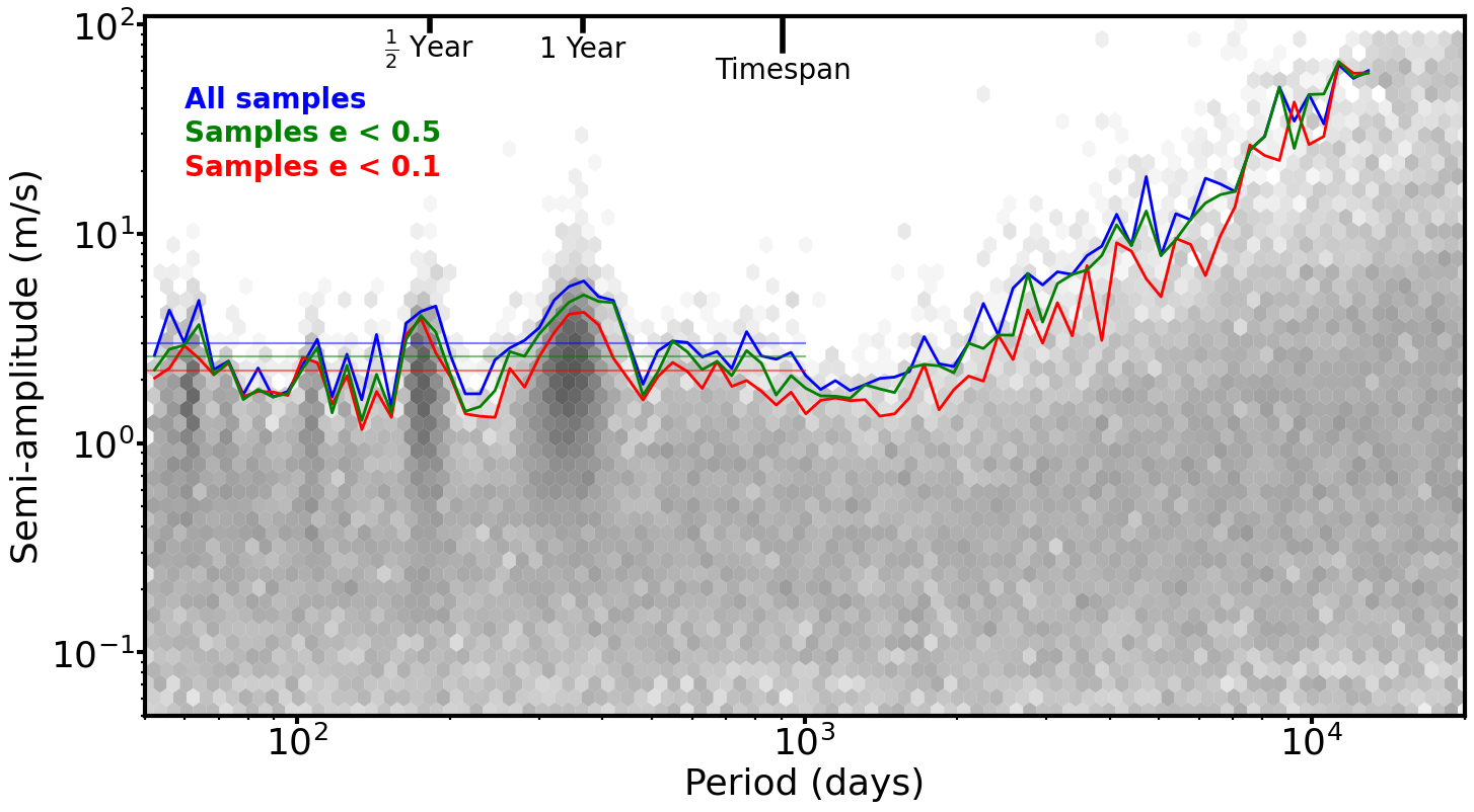
Figure 9: Hexbin plot of posterior samples and blue detection limit for J0310-31 as in figure 2. The Red and green lines here indicate the same limit calculated from posterior samples with eccentricities $<0.1$ and $<0.5$ respectively. Horizontal coloured lines show the mean semi-amplitude of the three coloured detection-limits out to $1000~{}\rm days$.

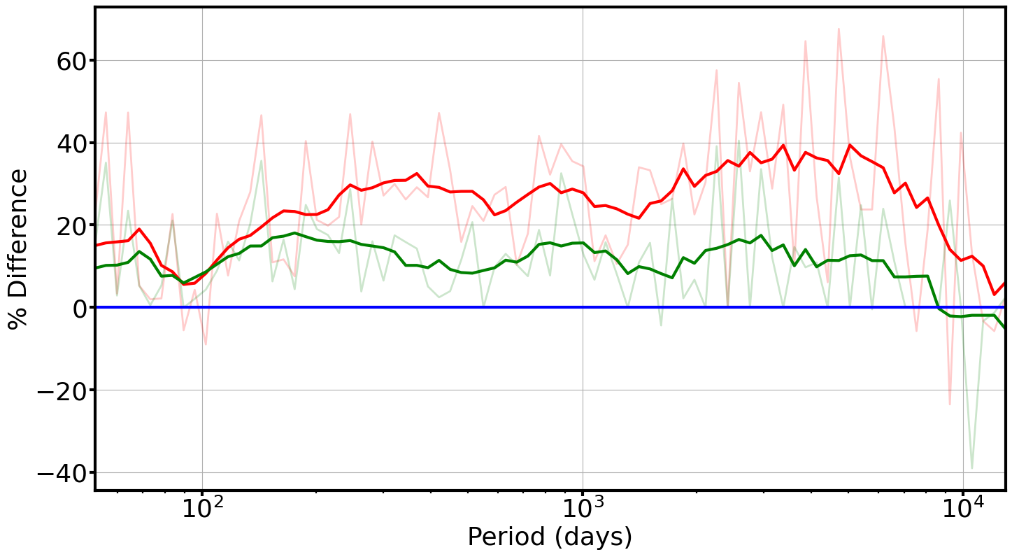
Figure 10: Plot of the percentage difference between detection limits calculated with all posterior samples, and posterior samples with eccentricities $<0.1$ and $<0.5$ in red and green respectively for J0310-31 from figure 9. Solid coloured lines represent a running mean taken on the faded coloured lines.

This exercise demonstrates the superiority of a diffusive nested sampler in establishing robust detection limits, which are crucial to infer the sensitivity of radial-velocity surveys, and consequently, the occurrence rates of exoplanets.

6 Conclusions

We analyse high-precision radial-velocities obtained as part of a large scale, ongoing, radial-velocity survey that seeks circumbinary planets using radial-velocities obtained with HARPS, ESPRESSO and SOPHIE, in both hemispheres, on single-lined eclipsing binaries. This survey is called BEBOP (Binaries Escorted By Orbiting Planets). We then detail an observing and Bayesian analysis protocol and test it on data collected for three single-lined binaries within the survey. Our analysis shows for the first time, a repeated ability to detect circumbinary planets with masses between Neptune’s and Saturn’s, for orbital periods within $1000$ days with as few as 25 spectra in the span of a year. Figure 11 displays a mass vs period plot of the detection limits from this work (blue) along with confirmed exoplanets (grey circles; NASA exoplanet archive), transiting circumbinary planets (magenta diamonds), and Solar System planets for comparison. This figure demonstrates our ability to detect sub-Saturn mass circumbinary planets at periods up to $1000$ days. Our data are able to detect a large fraction of currently known systems. We note though that many circumbinary planet detections made with eclipse timing variations are upper limits only.

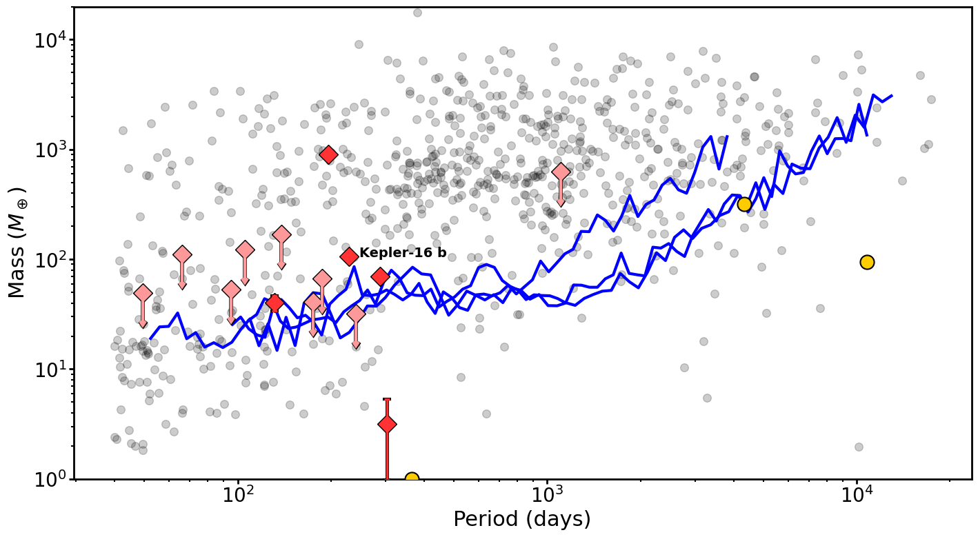
Figure 11: Mass vs period plot showing the three detection limits from this work as blue lines in comparison to confirmed exoplanets as grey circles, and transiting circumbinary planets as pink diamonds. Solar System planets are depicted as yellow dots for reference. Circumbinary planets in order of increasing period; Kepler-47 b, Kepler-413 b, TOI-1338 b, Kepler-38 b, Kepler-35 b, Kepler-64 b, Kepler-1661 b, Kepler-47 d, TIC-1729 b, Kepler-16 b, Kepler-453 b, Kepler-34 b, Kepler-47 c, Kepler-1647 b. Arrows illustrate planets with upper mass limits with the symbol placed to give a $2\sigma$ upper limit.

We also present a method to compute detection limits on radial-velocity data by using a diffusive nested sampler, without the need to assume circular orbits as is the norm. We then show that this method is superior than the usual injection-recovery tests. Assuming circular orbits when determining detection limits generates over-optimistic detection limits by an average of $\sim 1~{}\rm{m\,s^{-1}}$ ($24.7\%$) at periods $<1000~{}\rm day$, and up to $120~{}\rm M_{\oplus}$ at periods $>1000~{}\rm day$. We therefore strongly caution against assuming circular orbits when calculating detection limits, and suggest kima as a way for exoplanet surveys in general to extract accurate sensitivity limits and occurrence rates with fewer assumptions.

Thanks to the protocols and tests described in this paper, the BEBOP survey is now ready to produce circumbinary planet candidates following Bayesian evidence, and able to compute occurrence rates that can be compared to those already established from photometric methods (Armstrong et al., 2014; Martin & Triaud, 2014). Producing occurrence rates and upper limits on the occurrence of circumbinary planets will be done by simply combining all kima produced detection limits.

Data Availability

The data we used is available for download at the ESO public archive. Search for Prog.ID 099.C-0138 and 1101.C-0721.

Appendix A Injection and Recovery results and Radial Velocity data

Here we present the results of our insertion/recovery tests for each of our three target systems in tables 4 to 7, Numbers in the tables are Bayes factors calculated from our kima runs. We also present our RV data on the systems in tables 8 to 10.

Table 4: J0310-31 Keplerian insertion and recovery results

Semi-amplitudes			Periods
	$5.9\times P_{\rm bin}=74.59\rm{d}$	$12\times P_{\rm bin}=151.71\rm{d}$	$18\times P_{\rm bin}=227.57\rm{d}$	$30\times P_{\rm bin}=379.28\rm{d}$	$486.67\rm{d}$	$400\times P_{\rm bin}=5057.12\rm{d}$
$10\times\rm{RMS}=31.6\rm{m\,s^{-1}}$	-	-	-	-	-	inf
$3\times\rm{RMS}=9.48\rm{m\,s^{-1}}$	-	-	-	inf	-	$8.3$
$2\times\rm{RMS}=6.32\rm{m\,s^{-1}}$	inf	-	-	-	-	-
$1.5\times\rm{RMS}=4.74\rm{m\,s^{-1}}$	$39.7$	inf	-	$25.7$	$5946$	$0.8$
$1.25\times\rm{RMS}=3.95\rm{m\,s^{-1}}$	$3.2$	$5860$	$984.83$	-	$409.2$	-
$\rm{RMS}=3.16\rm{m\,s^{-1}}$	-	$1070.7$	$120.6$	$0.9$	$44.7$	-
$0.75\times\rm{RMS}=2.37\rm{m\,s^{-1}}$	-	$63.7$	$16.4$	-	$7.6$	-
$0.5\times\rm{RMS}=1.58\rm{m\,s^{-1}}$	-	$5.8$	$2.5$	-	-	-

Table 5: J0310-31 Rebound simulated N-body insertion and recovery results

Semi-amplitudes		Periods
	$5.9\times P_{\rm bin}=74.59\rm{d}$	$12\times P_{\rm bin}=151.71\rm{d}$	$486.67\rm{d}$
$2\times\rm{RMS}=6.32\rm{m\,s^{-1}}$	inf	-	-
$1.5\times\rm{RMS}=4.74\rm{m\,s^{-1}}$	$980$	inf	$1378.8$
$1.25\times\rm{RMS}=3.95\rm{m\,s^{-1}}$	$60.5$	inf	$264.5$
$\rm{RMS}=3.16\rm{m\,s^{-1}}$	$5.2$	$7020$	$41.5$
$0.75\times\rm{RMS}=2.37\rm{m\,s^{-1}}$	-	$217.4$	$7$
$0.5\times\rm{RMS}=1.58\rm{m\,s^{-1}}$	-	$11.3$	-

Table 6: J1540-09 Keplerian insertion and recovery results

Semi-amplitudes		Periods
	$5.9\times P_{\rm bin}=155.4\rm{d}$	$12\times P_{\rm bin}=316.06\rm{d}$	$486.67\rm{d}$	$999\rm{d}$
$3\times\rm{RMS}=11.25\rm{m\,s^{-1}}$	-	inf	-	-
$2.5\times\rm{RMS}=9.38\rm{m\,s^{-1}}$	-	inf	-	-
$2\times\rm{RMS}=7.5\rm{m\,s^{-1}}$	inf	$637.3$	inf	inf
$1.5\times\rm{RMS}=5.63\rm{m\,s^{-1}}$	$2811.7$	$14.5$	$1276.8$	$291$
$1.25\times\rm{RMS}=4.69\rm{m\,s^{-1}}$	$464.5$	$3.6$	$223.2$	$29.5$
$\rm{RMS}=3.75\rm{m\,s^{-1}}$	$72.6$	-	$23.2$	$3.7$
$0.75\times\rm{RMS}=2.81\rm{m\,s^{-1}}$	$8.4$	-	$3.6$	-
$0.5\times\rm{RMS}=1.88\rm{m\,s^{-1}}$	$1.5$	-	$0.9$	$0.7$

Table 7: J1928-38 Keplerian insertion and recovery results

Semi-amplitudes			Periods
	$5.1\times P_{\rm bin}=118.95\rm{d}$	$5.9\times P_{\rm bin}=137.61\rm{d}$	$8\times P_{\rm bin}=186.58\rm{d}$	$12\times P_{\rm bin}=279.87\rm{d}$	$486.67\rm{d}$
$5\times\rm{RMS}=14.8\rm{m\,s^{-1}}$	-	-	-	-	inf
$4\times\rm{RMS}=11.84\rm{m\,s^{-1}}$	-	inf	-	inf	inf
$3\times\rm{RMS}=8.88\rm{m\,s^{-1}}$	$2919$	$1362.6$	$6413$	inf	inf
$2\times\rm{RMS}=5.92\rm{m\,s^{-1}}$	$49.8$	$21$	$47.8$	$58.9$	$138.4$
$1.5\times\rm{RMS}=4.44\rm{m\,s^{-1}}$	-	$2.4$	-	$2.9$	$14.3$
$1.25\times\rm{RMS}=3.7\rm{m\,s^{-1}}$	$2.3$	-	$2.9$	-	-
$\rm{RMS}=2.96\rm{m\,s^{-1}}$	-	-	-	-	$2.4$

Table 8: Journal of Observations containing our HARPS data for J0310-31. Dates are given in BJD - 2,400,000. $V_{\rm rad}$ are the measured radial velocities with their uncertainties $\sigma_{V_{\rm rad}}$. FWHM is the Full With at Half Maximum of the Gaussian fitted to the cross correlation function, and contrast is its amplitude. bis. span is the span of the bisector slope. Uncertainties on FWHM and bis. span are $2\times\sigma_{V_{\rm rad}}$.

BJD	$V_{\rm rad}$	$\sigma_{V_{\rm rad}}$	FWHM	contrast	bis. span
	[km s-1]	[km s-1]	[km s-1]		[km s-1]
57943.892368	35.63948	0.00168	10.93301	31.049	0.02153
57944.923580	24.07411	0.00170	10.95037	31.088	0.02859
57945.885900	8.58139	0.00176	10.92966	31.091	0.01777
57946.876879	-6.07696	0.00185	10.92368	31.127	0.02400
57948.928854	18.35127	0.00199	10.92909	31.150	0.02186
57949.874496	32.36601	0.00376	10.93177	31.081	0.00910
57951.890174	46.34736	0.00245	10.92515	31.176	0.02321
57952.924664	48.32340	0.00184	10.93519	31.078	0.02634
57953.919672	47.93648	0.00224	10.93547	31.070	0.03302
57955.935525	40.23726	0.00148	10.92350	31.114	0.02441
57956.937097	31.73699	0.00242	10.90176	31.215	0.02218
57958.914371	1.85626	0.00250	10.90546	31.207	0.02907
57959.923988	-7.18919	0.00185	10.91742	31.126	0.02583
57960.925502	6.01245	0.00218	10.90108	31.196	0.01583
57962.941783	36.84076	0.00240	10.91809	31.103	0.02995
57967.873028	44.11773	0.00509	10.91773	31.108	0.03909
57968.862759	38.22158	0.00196	10.93156	31.078	0.02316
57970.834614	14.43370	0.00201	10.93765	31.107	0.02358
57971.887207	-3.14864	0.00203	10.90942	31.205	0.02815
57972.859262	-5.30070	0.00212	10.91962	31.137	0.02385
57973.874664	11.99910	0.00246	10.95580	31.021	0.03180
57974.855492	28.50055	0.00207	10.94437	31.112	0.01107
57979.910020	46.38457	0.00172	10.92281	31.125	0.03514
57980.907132	42.15442	0.00189	10.90393	31.195	0.03216
57981.912450	34.81087	0.00166	10.91749	31.142	0.02222
57993.897684	40.01640	0.00175	10.89351	31.237	0.02857
57994.868121	31.71289	0.00204	10.90854	31.176	0.01557
57995.913932	17.82943	0.00210	10.96594	31.005	0.02541
57996.900885	0.89748	0.00326	10.95410	31.062	0.01592
57998.846013	5.86085	0.00207	10.93080	31.128	0.03219
58000.814335	36.31122	0.00184	10.93406	31.090	0.02512
58001.825348	43.67481	0.00173	10.93076	31.065	0.03359
58002.875888	47.45290	0.00195	10.90752	31.138	0.02670
58008.865205	12.69217	0.00302	10.91455	31.160	0.02339
58010.891199	-4.13140	0.00193	10.93348	31.103	0.02658
58011.853533	12.96220	0.00186	10.93126	31.120	0.02981
58012.842881	29.29996	0.00194	10.93123	31.138	0.02439
58013.836117	39.60231	0.00231	10.89094	31.251	0.03815
58021.844325	6.77414	0.00237	10.88521	31.277	0.02190
58022.865563	-6.90867	0.00248	10.90068	31.182	0.02454
58023.861648	0.85340	0.00259	10.87215	31.286	0.01533
58026.843370	42.13524	0.00420	10.85961	31.323	0.03642
58027.851246	46.66027	0.00274	10.96376	30.975	0.03885
58292.935003	45.19779	0.00188	10.85673	31.290	0.03447
58295.939322	46.50750	0.00153	10.87040	31.248	0.02880
58336.906794	23.28586	0.00177	10.85126	31.372	0.01926
58338.851019	-6.42041	0.00176	10.85513	31.308	0.02670
58354.838158	36.55513	0.00227	10.87155	31.222	0.02979
58405.803761	39.90978	0.00460	10.85632	31.338	0.02138
58453.710487	0.74084	0.00138	10.90947	31.141	0.02863
58488.633260	23.11336	0.00169	10.86625	31.319	0.03055
58506.584524	36.86690	0.00139	10.91340	31.117	0.02021
58515.547144	-3.39784	0.00178	10.93431	31.069	0.02643
58519.564335	39.72933	0.00178	10.90851	31.130	0.02260
58692.848790	-6.41913	0.00154	10.90509	31.272	0.03065
58701.837991	40.38147	0.00167	10.91534	31.217	0.02113
58707.811668	23.67250	0.00297	10.91707	31.212	0.02879
58723.756754	47.90169	0.00143	10.91435	31.183	0.02889
58727.806796	35.08783	0.00171	10.91437	31.193	0.02715
58753.740711	28.24276	0.00219	10.92187	31.189	0.02651
58762.749317	48.28098	0.00163	10.91574	31.195	0.03644
58784.717703	36.78734	0.00202	10.89169	31.348	0.01632
58834.649676	29.63072	0.00147	10.95468	31.105	0.02506
58846.646146	19.74657	0.00175	10.95264	31.044	0.02730
58850.565260	48.32348	0.00127	10.92443	31.170	0.03143

Table 9: Journal of Observations containing our HARPS data for J1540-09. Columns are as in 8

BJD	$V_{\rm rad}$	$\sigma_{V_{\rm rad}}$	FWHM	contrast	bis. span
	[km s-1]	[km s-1]	[km s-1]		[km s-1]
57863.886017	-34.04435	0.00284	8.28287	34.515	0.03306
57865.839152	-43.91032	0.00232	8.29807	34.391	0.02892
57872.835002	-77.11478	0.00297	8.27285	34.583	0.02351
57875.857985	-74.41238	0.00535	8.29200	34.511	0.01455
57879.754279	-61.45253	0.00319	8.28987	34.441	0.03454
57923.573674	-73.41843	0.00409	8.25559	34.767	0.03070
57934.687091	-51.51693	0.00429	8.25721	34.747	0.03096
57942.695102	-33.38362	0.00351	8.30337	34.065	0.03405
57944.691282	-42.89582	0.00281	8.31499	34.146	0.02189
57945.660293	-49.29063	0.00272	8.30231	34.259	0.03662
57948.624456	-68.11507	0.00343	8.28781	34.553	0.01667
57951.646824	-76.94824	0.00745	8.26195	34.595	0.03799
57959.584739	-57.97578	0.00382	8.28518	34.608	0.03248
57964.618682	-36.33938	0.00429	8.31324	34.080	0.04210
57969.547587	-35.17730	0.00473	8.27743	34.448	0.04891
57979.581918	-76.95182	0.00272	8.29949	34.246	0.02375
57996.529560	-38.13035	0.00324	8.31348	34.277	0.04163
58001.510009	-69.13364	0.00302	8.30714	34.214	0.02582
58008.470052	-72.09597	0.02062	8.26838	34.398	0.07094
58012.493882	-56.95128	0.00442	8.28094	34.427	0.01261
58258.703952	-33.23617	0.00278	8.24429	34.880	0.03156
58272.646623	-69.65691	0.00254	8.25571	34.828	0.02267
58276.707794	-53.23456	0.00213	8.27952	34.650	0.02728
58278.649982	-44.46367	0.00270	8.26452	34.718	0.01897
58286.693559	-40.52268	0.00279	8.25444	34.814	0.04001
58291.571082	-70.64953	0.00291	8.26216	34.799	0.03911
58301.682725	-59.27470	0.00501	8.26292	34.601	0.04623
58334.515634	-32.95173	0.00224	8.26416	34.732	0.03756
58340.485380	-47.58266	0.00313	8.23341	34.979	0.02739
58356.492448	-49.72878	0.00241	8.25519	34.600	0.02249
58521.884427	-32.68384	0.00572	8.24942	34.789	0.03390
58548.884978	-34.78751	0.00269	8.27384	34.712	0.02978
58565.835269	-55.89578	0.00223	8.29513	34.526	0.02256
58584.849299	-77.25342	0.00212	8.30491	34.430	0.01920
58600.898483	-32.67798	0.00320	8.32099	34.343	0.03645
58611.764016	-76.90855	0.00584	8.28568	34.680	0.02539
58615.819016	-66.97010	0.00252	8.29986	34.518	0.01559
58644.693557	-56.58981	0.00235	8.29114	34.526	0.03632
58660.683192	-72.15472	0.00377	8.27641	34.651	0.03250
58673.679701	-44.66300	0.00441	8.27281	34.705	0.01648
58914.890985	-31.32791	0.00276	8.27327	34.612	0.03724

Table 10: Journal of Observations containing our HARPS data for J1928-38. Columns are as in 8

BJD	$V_{\rm rad}$	$\sigma_{V_{\rm rad}}$	FWHM	contrast	bis. span
	[km s-1]	[km s-1]	[km s-1]		[km s-1]
58273.834134	32.80650	0.00217	7.04698	48.100	-0.00888
58278.843949	17.69958	0.00355	7.07692	47.503	-0.00764
58284.752885	-1.49688	0.00232	7.04283	48.268	-0.00407
58288.745112	9.82687	0.00190	7.04846	48.270	-0.00610
58292.729051	25.70995	0.00326	7.02329	48.428	0.00265
58293.708035	28.62785	0.00290	7.03782	47.844	0.00469
58311.790430	8.67845	0.00209	7.05597	47.813	-0.00506
58334.565596	6.49932	0.00184	7.05307	48.138	0.00278
58338.621368	23.08744	0.00361	7.03939	48.057	-0.00714
58346.585986	27.43032	0.00176	7.05339	48.206	-0.01117
58355.645102	-0.30616	0.00228	7.06381	47.595	-0.00554
58550.896768	30.15923	0.00242	7.07663	47.847	-0.00196
58556.881115	26.03178	0.00374	7.06599	48.034	0.00072
58556.901788	25.94663	0.00338	7.06541	48.122	-0.01728
58564.890277	-1.28170	0.00189	7.06720	47.828	-0.00538
58586.899133	-1.30374	0.00203	7.07108	47.947	-0.00910
58612.855107	1.20469	0.00577	7.07242	47.921	-0.01711
58637.829855	6.75596	0.00257	7.07361	47.829	-0.00782
58643.837284	29.35475	0.00212	7.09607	47.618	0.00213
58664.803891	21.81645	0.00247	7.11147	47.332	0.00270
58667.703897	30.57137	0.00231	7.08125	47.868	0.00740
58670.740859	32.53833	0.00203	7.07063	47.896	-0.00829
58700.663044	7.52499	0.00187	7.07861	47.860	-0.00283
58726.538304	-0.92379	0.00392	7.05509	47.966	-0.00253
58740.520279	32.68685	0.00267	7.06985	47.567	-0.01475

References

- Armstrong et al. (2014) Armstrong D. J., Osborn H. P., Brown D. J. A., Faedi F., Gómez Maqueo Chew Y., Martin D. V., Pollacco D., Udry S., 2014, MNRAS, 444, 1873
- Arras et al. (2012) Arras P., Burkart J., Quataert E., Weinberg N. N., 2012, MNRAS, 422, 1761
- Baranne et al. (1996) Baranne A., et al., 1996, A&AS, 119, 373
- Bonfils et al. (2011) Bonfils X., et al., 2011, A&A, 528, A111
- Bonfils et al. (2013) Bonfils X., et al., 2013, A&A, 549, A109
- Borucki & Summers (1984) Borucki W. J., Summers A. L., 1984, Icarus, 58, 121
- Brewer (2014) Brewer B. J., 2014, arXiv e-prints, p. arXiv:1411.3921
- Brewer & Donovan (2015) Brewer B. J., Donovan C. P., 2015, MNRAS, 448, 3206
- Brewer et al. (2011) Brewer B. J., Pártay L. B., Csányi G., 2011, Statistics and Computing, 21, 649
- Coffinet et al. (2019) Coffinet A., Lovis C., Dumusque X., Pepe F., 2019, A&A, 629, A27
- Correia et al. (2005) Correia A. C. M., Udry S., Mayor M., Laskar J., Naef D., Pepe F., Queloz D., Santos N. C., 2005, A&A, 440, 751
- Correia et al. (2010) Correia A. C. M., et al., 2010, A&A, 511, A21
- Couetdic et al. (2010) Couetdic J., Laskar J., Correia A. C. M., Mayor M., Udry S., 2010, A&A, 519, A10
- Cumming & Dragomir (2010) Cumming A., Dragomir D., 2010, MNRAS, 401, 1029
- Cumming et al. (2008) Cumming A., Butler R. P., Marcy G. W., Vogt S. S., Wright J. T., Fischer D. A., 2008, PASP, 120, 531
- Doolin & Blundell (2011) Doolin S., Blundell K. M., 2011, MNRAS, 418, 2656
- Doyle et al. (2011) Doyle L. R., et al., 2011, Science, 333, 1602
- Dvorak et al. (1989) Dvorak R., Froeschle C., Froeschle C., 1989, A&A, 226, 335
- Endl et al. (2002) Endl M., Kürster M., Els S., Hatzes A. P., Cochran W. D., Dennerl K., Döbereiner S., 2002, A&A, 392, 671
- Everhart (1985) Everhart E., 1985, An efficient integrator that uses Gauss-Radau spacings. p. 185, doi:10.1007/978-94-009-5400-7_17
- Faria et al. (2018) Faria J. P., Santos N. C., Figueira P., Brewer B. J., 2018, The Journal of Open Source Software, 3, 487
- Faria et al. (2020) Faria J. P., et al., 2020, A&A, 635, A13
- Feroz et al. (2011) Feroz F., Balan S. T., Hobson M. P., 2011, MNRAS, 415, 3462
- Foreman-Mackey (2016) Foreman-Mackey D., 2016, The Journal of Open Source Software, 1, 24
- Gaia Collaboration (2018) Gaia Collaboration 2018, VizieR Online Data Catalog, p. I/345
- Gregory (2005) Gregory P. C., 2005, ApJ, 631, 1198
- Høg et al. (2000) Høg E., et al., 2000, A&A, 355, L27
- Holman & Wiegert (1999) Holman M. J., Wiegert P. A., 1999, AJ, 117, 621
- Howard et al. (2010) Howard A. W., et al., 2010, Science, 330, 653
- Jeffreys (1961) Jeffreys H., 1961, Theory of probability. Oxford University Press
- Kipping (2013) Kipping D. M., 2013, MNRAS, 434, L51
- Konacki et al. (2009) Konacki M., Muterspaugh M. W., Kulkarni S. R., Hełminiak K. G., 2009, ApJ, 704, 513
- Konacki et al. (2010) Konacki M., Muterspaugh M. W., Kulkarni S. R., Hełminiak K. G., 2010, ApJ, 719, 1293
- Kostov et al. (2013) Kostov V. B., Mccullough P. R., Hinse T. C., Tsvetanov Z. I., Hébrard G., Díaz R. F., Deleuil M., Valenti J. A., 2013, The Astrophysical Journal, 770, 52
- Kostov et al. (2014) Kostov V. B., et al., 2014, The Astrophysical Journal, 784, 14
- Kostov et al. (2016) Kostov V. B., et al., 2016, The Astrophysical Journal, 827, 86
- Kostov et al. (2020) Kostov V. B., et al., 2020, AJ, 159, 253
- Kostov et al. (2021) Kostov V. B., et al., 2021, arXiv e-prints, p. arXiv:2105.08614
- Kumaraswamy (1980) Kumaraswamy P., 1980, Journal of Hydrology, 46, 79
- Lovis & Pepe (2007) Lovis C., Pepe F., 2007, A&A, 468, 1115
- Mardling (2013) Mardling R. A., 2013, MNRAS, 435, 2187
- Martin (2017) Martin D. V., 2017, MNRAS, 465, 3235
- Martin (2018) Martin D. V., 2018, Populations of Planets in Multiple Star Systems. p. 156, doi:10.1007/978-3-319-55333-7_156
- Martin (2019) Martin D. V., 2019, MNRAS, 488, 3482
- Martin & Triaud (2014) Martin D. V., Triaud A. H. M. J., 2014, A&A, 570, A91
- Martin et al. (2019) Martin D. V., et al., 2019, A&A, 624, A68
- Mayor et al. (2003) Mayor M., et al., 2003, The Messenger, 114, 20
- Mayor et al. (2009) Mayor M., et al., 2009, A&A, 507, 487
- Mayor et al. (2011) Mayor M., et al., 2011, arXiv e-prints, p. arXiv:1109.2497
- McInnes et al. (2017) McInnes L., Healy J., Astels S., 2017, The Journal of Open Source Software, 2
- Munari et al. (2014) Munari U., et al., 2014, AJ, 148, 81
- Orosz et al. (2012a) Orosz J. A., et al., 2012a, Science, 337, 1511
- Orosz et al. (2012b) Orosz J. A., et al., 2012b, ApJ, 758, 87
- Orosz et al. (2019) Orosz J. A., et al., 2019, AJ, 157, 174
- Pepe et al. (2002a) Pepe F., et al., 2002a, The Messenger, 110, 9
- Pepe et al. (2002b) Pepe F., Mayor M., Galland F., Naef D., Queloz D., Santos N. C., Udry S., Burnet M., 2002b, A&A, 388, 632
- Perruchot et al. (2008) Perruchot S., et al., 2008, in McLean I. S., Casali M. M., eds, Society of Photo-Optical Instrumentation Engineers (SPIE) Conference Series Vol. 7014, Ground-based and Airborne Instrumentation for Astronomy II. p. 70140J, doi:10.1117/12.787379
- Pollacco et al. (2006) Pollacco D. L., et al., 2006, PASP, 118, 1407
- Quarles et al. (2018) Quarles B., Satyal S., Kostov V., Kaib N., Haghighipour N., 2018, ApJ, 856, 150
- Queloz et al. (2001) Queloz D., et al., 2001, A&A, 379, 279
- Rein & Liu (2012) Rein H., Liu S. F., 2012, A&A, 537, A128
- Rein & Spiegel (2015) Rein H., Spiegel D. S., 2015, MNRAS, 446, 1424
- Robert E. Kass; Adrian E. Raftery (1995) Robert E. Kass; Adrian E. Raftery 1995, Journal of the American Statistical Association, 90, 773
- Rosenthal et al. (2021) Rosenthal L. J., et al., 2021, arXiv e-prints, p. arXiv:2105.11583
- Sabotta et al. (2021) Sabotta S., et al., 2021, arXiv e-prints, p. arXiv:2107.03802
- Santos et al. (2002) Santos N. C., et al., 2002, A&A, 392, 215
- Schneider (1994) Schneider J., 1994, Planet. Space Sci., 42, 539
- Schwamb et al. (2013) Schwamb M. E., et al., 2013, The Astrophysical Journal, 768, 127
- Socia et al. (2020) Socia Q. J., et al., 2020, AJ, 159, 94
- Swayne et al. (2021) Swayne M. I., et al., 2021, arXiv e-prints, p. arXiv:2106.07276
- Sybilski et al. (2013) Sybilski P., Konacki M., Kozłowski S. K., Hełminiak K. G., 2013, MNRAS, 431, 2024
- Triaud (2018) Triaud A. H. M. J., 2018, The Rossiter-McLaughlin Effect in Exoplanet Research. p. 2, doi:10.1007/978-3-319-55333-7_2
- Triaud et al. (2013) Triaud A. H. M. J., et al., 2013, A&A, 549, A18
- Triaud et al. (2017) Triaud A. H., et al., 2017, A&A, 608, A129
- Trotta (2008) Trotta R., 2008, Contemporary Physics, 49, 71
- Welsh et al. (2012) Welsh W. F., et al., 2012, Nature, 481, 475
- Welsh et al. (2015) Welsh W. F., et al., 2015, ApJ, 809, 26
- Wittenmyer et al. (2006) Wittenmyer R. A., Endl M., Cochran W. D., Hatzes A. P., Walker G. A. H., Yang S. L. S., Paulson D. B., 2006, AJ, 132, 177
- Zechmeister et al. (2009) Zechmeister M., Kürster M., Endl M., 2009, A&A, 505, 859
- Zucker & Alexander (2007) Zucker S., Alexander T., 2007, ApJ, 654, L83