Supplemental Material:
“Quasiparticle poisoning in trivial and topological Josephson junctions”

I The low-energy spectrum of a Josephson junction based on a proximitized semiconducting nanowire with strong SOI close to the phase transition

In this section we provide a detailed analysis of the low-energy spectrum of a topological Josephson junction (JJ). We analyze the scaling of the phase potential amplitude ($E_{J}$ for trivial phase and $E_{M}$ for topological) with the normal state transmission amplitude $D_{N}$ to validate our analysis of phase evolution after the parity switch in the main text. Our starting point is a linearization procedure Klinovaja and Loss (2012) with subsequent calculation of the low-energy spectrum San-Jose et al. (2013); Murthy et al. (2020) for a JJ based on a semiconducting nanowire with strong Rashba spin-orbit interaction (SOI) of strength $\alpha$, as in this regime the junction is in the Andreev limit ($\Delta\ll E_{F}\sim m\alpha^{2}$, where $E_{F}$ is the Fermi energy measured from the bottom of conduction band and is set by the characteristic energy of SOI $\sim m\alpha^{2}$, where $m$ is the effective electron band mass). Two further ingredients are the Zeeman field $V_{Z}\ll m\alpha^{2}$ and the proximity gap $\Delta$. An additional assumption we make to simplify the analysis is that the Fermi level is exactly in the middle of the Zeeman gap. For the case of a short junction region, modelled as a delta-function barrier, one can write down the equation determining the bound states as Murthy et al. (2020):

$$\Lambda(E,\phi,D_{N},V_{Z})=0,$$ (1)

where $\Lambda$ is given by

$$\Lambda(E,\phi,D_{N},V_{Z})=\Lambda_{0}(E,\phi,V_{Z})+(1-D_{N})\Lambda_{1}(E,\phi,V_{Z})+(1-D_{N})^{2}\Lambda_{2}(E,\phi,V_{Z})+D_{N}\Lambda_{\gamma}(E,\phi,V_{Z})\sin^{2}\gamma;$$ (2)

$$\Lambda_{0}(E,\phi,V_{Z})=\left[\Delta^{2}\cos^{2}\frac{\phi}{2}-E^{2}\right]\left[\sqrt{\Delta_{-}^{2}-E^{2}}\sqrt{\Delta_{+}^{2}-E^{2}}\left(1+\cos^{2}\frac{\phi}{2}\right)-\left(E^{2}+\Delta_{-}\Delta_{+}\right)\sin^{2}\frac{\phi}{2}\right],$$ (3)

$$\Lambda_{1}(E,\phi,V_{Z})=\left[\left(E^{2}+\Delta_{-}\Delta_{+}\right)\left(2\Delta^{2}\cos^{2}\frac{\phi}{2}-E^{2}\right)-2\Delta^{2}E^{2}\right]\sin^{2}\frac{\phi}{2}$$

$$+\sqrt{\Delta^{2}-E^{2}}\sqrt{\Delta_{-}^{2}-E^{2}}\left[\Delta\Delta_{+}\cos^{2}\frac{\phi}{2}-E^{2}\right]+\sqrt{\Delta^{2}-E^{2}}\sqrt{\Delta_{+}^{2}-E^{2}}\left[\Delta\Delta_{-}\cos^{2}\frac{\phi}{2}-E^{2}\right]$$

$$-\sqrt{\Delta_{-}^{2}-E^{2}}\sqrt{\Delta_{+}^{2}-E^{2}}\left[2\Delta^{2}\cos^{4}\frac{\phi}{2}-E^{2}\left(1+\cos^{2}\frac{\phi}{2}\right)\right],$$ (4)

$$\Lambda_{2}(E,\phi,B)=\Delta^{2}\left(E^{2}+\Delta_{-}\Delta_{+}\right)\sin^{4}\frac{\phi}{2}+\frac{1}{2}\left(\Delta_{-}\Delta_{+}-E^{2}\right)\left[\Delta^{2}\cos\phi-E^{2}\right]$$

$$-\frac{1}{2}B^{2}E^{2}-\frac{1}{2}\sqrt{\Delta^{2}-E^{2}}\sqrt{\Delta_{-}^{2}-E^{2}}\left[\Delta\Delta_{+}\cos\phi-E^{2}\right]-\frac{1}{2}\sqrt{\Delta^{2}-E^{2}}\sqrt{\Delta_{+}^{2}-E^{2}}\left[\Delta\Delta_{-}\cos\phi-E^{2}\right]$$

$$+\frac{1}{2}\sqrt{\Delta_{-}^{2}-E^{2}}\sqrt{\Delta_{+}^{2}-E^{2}}\left[\Delta^{2}\left(1-\frac{1}{2}\sin^{2}\phi\right)-E^{2}\right],$$ (5)

$$\Lambda_{\gamma}(E,\phi,V_{Z})=\left[\Delta^{2}\cos^{2}\frac{\phi}{2}-E^{2}\right]\left[-\sqrt{\Delta_{-}^{2}-E^{2}}\sqrt{\Delta_{+}^{2}-E^{2}}+\Delta_{-}\Delta_{+}-E^{2}\right].$$ (6)

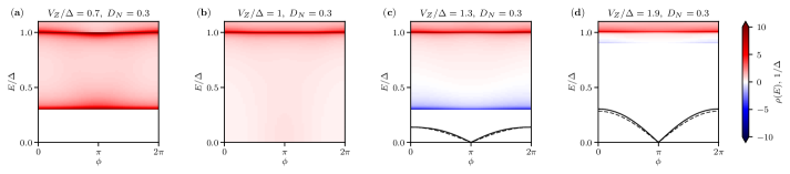
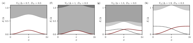
Figure 1: Upper panels (a-d) show the single-particle spectrum at different values of Zeeman field $V_{Z}$ as function of phase $\phi$, corresponding to (a) trivial phase, (b) transition, and (c, d) topological phase. The colour over $|V_{Z}-\Delta|$ indicates the local density of states, while the black line below the gap corresponds to the bound state. In the topological phase (c, d) the dashed line corresponds to our analytical solution; we note that both parity solutions are depicted, one before $\pi$ another one after $\pi$. In the trivial phase (a) the bound state is absent for small $D_{N}=0.3$. The lower panel (e-h) shows the many-body spectrum of the junction vs. $\phi$ at different values of $V_{Z}$; the solid red line represents the ground state, the grey area is the continuum, and the dotted line represents an odd-parity state. In the trivial state (e) at $V_{Z}/\Delta=0.7$ the spectrum consists of the ground state and no discrete excited states up to the continuum (since there are no bound states); panel (f) shows the gapless spectrum at the phase transition; panel (g) corresponds to the topological phase at $V_{Z}/\Delta=1.3$, each second local minimum of the ground state is suppressed by a $4\pi$-periodic contribution, and panel (h) corresponds to the topological phase at $V_{Z}/\Delta=1.9$, where only $4\pi$-periodic local minima remain.

Here $\Delta_{-}=|\Delta-V_{Z}|$, the gap of the system, and $\Delta_{+}=\Delta+V_{Z}$ are introduced for simplicity, $\gamma$ is the forward scattering phase, for the toy model of a point-like potential it is given by

$$\gamma=-\arctan\sqrt{\frac{1-D_{N}}{D_{N}}}.$$ (7)

In this system the continuum consisting of the scattering states above $|\Delta-V_{Z}|$ (or more generally the smallest gap in the system $\mathrm{min}\left[|\Delta-V_{Z}|,\Delta\right]$) should be taken into account, as it possesses a phase dependence (one can see it as a bound state merged into the continuum) and, therefore, affects the spectrum of the system already starting from the ground state. This phase-dependent contribution to the density of states in the continuum can be calculated via the same $\Lambda$ expression Murthy et al. (2020):

$$\delta\rho(E,\phi)=\frac{1}{2\pi{i}}\frac{\partial}{\partial{E}}\frac{\Lambda^{*}(E,\phi,D_{N},V_{Z})}{\Lambda(E,\phi,D_{N},V_{Z})}.$$ (8)

The spectrum in the high-transparency limit was analyzed in San-Jose et al. (2013); Murthy et al. (2020).

Here, we study the low-transparency limit, as it allows us to perform some estimations due to the simple cosine dependences on the phase (tunneling regime). To begin with, we expand

$$\sin^{2}\gamma=1-\frac{D_{N}}{4}+O(D_{N}^{2}).$$ (9)

Searching for the zeroes of $\Lambda(E,\phi,D_{N},V_{Z})$ numerically, we see that the lowest ABS sticks to the gap, as expected, while the second ABS is completely merged with the continuum. The remaining ABS does not scale linearly with $D_{N}$, as in a trivial spin-degenerate ABS, but rapidly decays to zero with increase of $V_{Z}$. For each transmission amplitude $D_{N}$ there is a value $V_{Z}^{bs}$, starting from which there is no bound state in the trivial phase, this value can be found as a solution of the equation:

$$\Lambda(\Delta-V_{Z}^{bs},\pi,D_{N},V_{Z}^{bs})=0.$$ (10)

From the numerical analysis we can conclude that in the low-transparency case, the system has no bound states in a large vicinity of the phase transition, i.e. for $D_{N}=0.3$ the bound state disappears already at $V_{Z}=0.4328\Delta$. Therefore, we state that in a large vicinity of the transition all the phase dependences of the low-energy spectrum are determined by the phase-dependent density of states of the continuum, which allows us to state (in the main text) that there are no effects due to quasiparticle poisoning around the phase transition. Moreover, what is also interesting is that the total contribution (ABSs plus continuum) to the ground state in the trivial phase has a weak dependence on the magnetic field, which can be seen as if the continuum is acquiring a phase-dependent contribution from the ABSs merged into it. On the contrary, in the topological phase the only bound state amplitude scales as $D_{N}$ at low transparency, as the continuum is gapped away from the bound state. We have calculated the amplitude in the low transparency limit expanding $\Lambda(E,\phi,D_{N},V_{Z})$ analytically in $D_{N}$ and $E/(V_{Z}-\Delta)$ (see Fig. 2):

$$E\approx 2\frac{D_{N}\Delta}{V_{Z}}(V_{Z}-\Delta)\cos\frac{\phi}{2},$$ (11)

which is Eq. (4) in the main text. What is a bit counterintuitive at first sight is the linear scaling with $D_{N}$, as naively it is expected to be the same as in Ref. Fu and Kane (2009) $\sim\sqrt{D_{N}}$, which corresponds to the single electron tunneling amplitude. The reason for this is that in Ref. Fu and Kane (2009) the edge states are supposed to carry only two helical modes, which is valid only at large Zeeman fields $V_{Z}\gg\Delta$ Murthy et al. (2020), where our formula is not applicable, as the SOI energy is no longer the largest energy scale in the system.

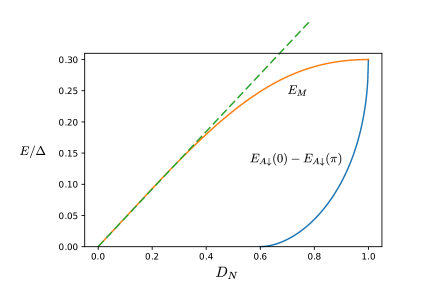
Figure 2: Dependence of the bound state amplitude on transmission amplitude $D_{N}$. The orange branch corresponds to the topological phase $V_{Z}=1.3\Delta$, green dashed line is the analytical solution for low transparency; blue curve represents lowest ABS energy amplitude in the trivial phase for $V_{Z}=0.7\Delta$ (difference of ABS energy at $\phi=0$, when it touches the gap, and at $\phi=\pi$, when it is minimal). One can see that there is no ABS for low $D_{N}$, then starting from some value of transmission the bound state amplitude grows up to the bulk gap size $\Delta_{c}=\Delta-V_{Z}$.

Now we can write down the many-body spectrum of the system. For the low-energy states it is described by the occupation of bound states and continuum states below the superconducting gap $\Delta$:

$$H(\phi)=E_{b}(\phi)\left(n_{b}-\frac{1}{2}\right)+\sum_{i}E_{i}(\phi)\left(n_{i}-\frac{1}{2}\right)+H_{0},$$ (12)

where $E_{b}(\phi)$ is the bound state energy - either the lowest ABS in the trivial phase, or the bound state formed by two MBSs in the topological phase - $n_{b}$ is the occupation of the state; $|\Delta-V_{Z}|<E_{i}(\phi)<\Delta$ are the energies of the continuum states, $n_{i}$ is the number operator for fermions in each continuum state; $H_{0}$ is the phase-independent contribution. From the numerical solution we deduce that a parity switch close to the phase transition can only slightly modify the phase dependence of the system energy, as $E_{b}$ is suppressed for small $D_{N}$ or absent completely (all ABSs merging with continuum) and the main contribution to the low-energy spectrum comes from the scattering states in the continuum between the system gap $\Delta-V_{Z}$ and superconducting gap $\Delta$. On the other side, deep inside the topological phase, a $4\pi$-periodic bound state contribution dominates over the continuum contribution and, therefore, each parity switching event significantly changes the phase dependence of the system energy. The full picture of the spectrum evolution with Zeeman field can be seen in Fig. 1.

In a junction based on proximitized semiconducting nanowires with weak SOI, the Andreev limit is violated. Therefore, the regime is very hard to analyze analytically, however, we expect the qualitative behaviour of the system to remain the same. At zero Zeeman field two degenerate ABSs are present, the significant difference with strong SOI regime is the absence of zero-energy crossings at $\phi=\pi$ even for perfect transparency of the junction $D_{N}=1$. In the presence of an external magnetic field, the ABSs split and get different amplitudes in the phase, as well as a phase-dependent contributions from the continuum appear. Close to the topological phase transition the continuum contribution to the ground state is dominating (on both sides of the transition). In the topological phase one would get $4\pi$-periodic term due to hybridization of the two MBSs on the junction, however, the amplitude is determined not by the superconducting gap and Zeeman field $\Delta_{c}=V_{Z}-\Delta$, as in the strong SOI limit, but also by the SOI energy scale $E_{SO}=m\alpha^{2}/2$ Klinovaja and Loss (2012); Cayao et al. (2017):

$$\Delta_{c}\approx 2\sqrt{\frac{E_{SO}}{V_{Z}}}\Delta.$$ (13)

Nevertheless, deep inside the topological phase the MBS contribution is again dominating in the phase potential, therefore, the spectrum has the same features which are crucial for the observation of the effects discussed in the main text.

II Finite-size effects in the topological phase

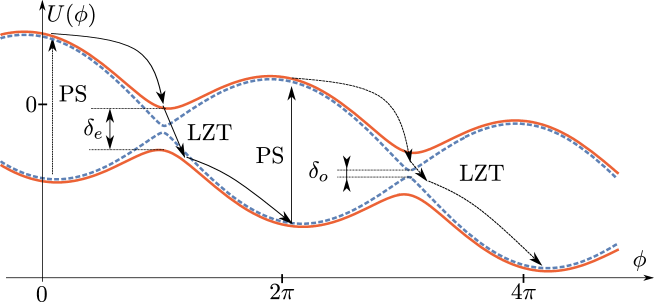
Figure 3: The phase potential $U$ for two different parities (solid red line for even parity and dashed blue for odd) as function of phase $\phi$. Here we have chosen smaller splittings in the odd state than in the even state $\delta_{o}<\delta_{e}$, however, this does not need to be the case in general. Arrows correspond to phase evolution: vertical arrows marked with PS correspond to parity switches, arrows along the phase potential branches represent phase relaxation, LZT represents Landau-Zener transitions at the anticrossings. All the solid arrows correspond to phase evolution in the even state (or starting in even state for phase switch), dashed arrows to that of the odd state.

Here we analyze finite-size effects in the setup discussed in the main text and show that they do not significantly affect the proposed measurement. If there is a finite overlap with the MBSs on the outer edges of the topological part of the system, crossings at $\phi\approx(2k+1)\pi$ turn into anticrossings Pikulin and Nazarov (2012); Domínguez et al. (2012). Strictly speaking, there are now four energy levels instead of two:

$$E^{e}_{\pm}=\pm\frac{1}{2}\sqrt{E_{M}^{2}\cos^{2}\frac{\phi}{2}+(\delta_{L}+\delta_{R})^{2}},$$ (14)

$$E^{o}_{\pm}=\pm\frac{1}{2}\sqrt{E_{M}^{2}\cos^{2}\frac{\phi}{2}+(\delta_{L}-\delta_{R})^{2}},$$ (15)

where the superscript $e$ ($o$) stands for even (odd) parity solution, $\delta_{L}$ ($\delta_{R}$) is the coupling with the MBS on the left (right) edge of the topological nanowire. What is important now is that the parity is the parity of the superposition of all four MBSs. Another issue worth mentioning is that $\delta_{R}$ and $\delta_{L}$ depend on the exact geometry of the nanowires forming the junction and can be both positive or negative. However, for each parity (which is fixed between parity switching events) the spectrum consist of two branches with fixed anticrossing $\delta=\left|\delta_{L}\pm\delta_{R}\right|$ (the sign of it being defined by the parity). If the phase evolution (relaxation) is fast enough in comparison to the splitting $\delta$ at the anticrossing, $\tau_{2\pi}^{-1}\gg\delta^{2}/(2E_{M})$, a Landau-Zener transition (LZT) would let the system reach the lower branch and relax to a new $2\pi$-shifted minimum as in the perfectly $4\pi$-periodic case. However, if $R/R_{Q}\ll\delta^{2}/E_{M}^{2}$, which can be the case for strongly overdamped junctions and for finite $\delta$, no LZT occurs and the state stays in the upper branch, thereby relaxing to the minimum at the anticrossing, giving rise to a voltage pulse of size $V=\frac{1}{2e}\frac{\pi}{\tau_{\pi}}$, where $\tau_{\pi}$ is the characteristic time for relaxation to a new $\pi$-shifted minimum. The next quasiparticle poisoning event will transfer the state to the lower branch with subsequent relaxation to a minimum, which also results in a $\pi$ phase shift. Therefore, the average voltage will be twice smaller than in the $4\pi$-periodic case [cf. Eq. (6) in the main text]:

$$\langle{V}\rangle\approx\frac{1}{2e}\frac{\pi}{\tau_{qp}^{top}}.$$ (16)

If one can fine tune the overlap of the MBSs so that in one parity state the splitting $\delta$ is large enough to suppress LZT and in another parity state it is very small (i.e. $\delta_{L}\approx\delta_{R}$ and $R/R_{Q}\ll 4\delta_{L}^{2}/E_{M}^{2}$), then it is possible to achieve an intermediate regime, where the average voltage is

$$\langle{V}\rangle\approx\frac{1}{2e}\frac{3\pi}{2\tau_{qp}^{top}},$$ (17)

as after the parity switch the phase will relax by $\pi$ or $2\pi$ depending on the parity.

III Voltage Pulses in the trivial phase

In this section we provide a detailed description of the quasiparticle poisoning effect in the trivial phase to supplement the discussion of the effect in the main text. If the junction is in the trivial phase, quasiparticles can be trapped in ABSs or recombine pairwise into the condensate of Cooper pairs. Both processes are rather slow (in comparison to getting trapped in the topological phase). Recombination is slow, since the recombination rate depends on the quasiparticle density quadratically ($\sim x^{2}_{qp}$, where $x_{qp}=n_{qp}/n_{cp}\ll 1$ is the ratio of quasiparticle density and Cooper pair density), while the trapping rate to an ABS is low due to the small energy gap between the ABS energy and the continuum edge. If the bias current is zero, $I=0$, the bound states touch the continuum edge at the phase values corresponding to the minima of the phase potential $\phi_{min}=2\pi k$ ($k$ is integer), therefore, a quasiparticle cannot be trapped. For small bias current, $I\ll I_{c}$, the minima of the phase potential are slightly shifted, i.e. $\phi_{min}\approx 2\pi k+\frac{I}{2eE_{J}}$, which results in a small energy gap between the continuum edge and the bound state $\epsilon=I^{2}/(4e^{2}E_{J})\ll\Delta$ at $\phi_{min}$, which allows quasiparticle trapping in the bound states. As a result, at zero magnetic field, when a quasiparticle is trapped in an ABS, the only conducting channel will get poisoned, which would result in a running (resistive) state with voltage $V=IR$. Subsequently the system will relax back to the ground state due to recombination of the trapped quasiparticle with a quasiparticle from the continuum on a time scale $\tau_{r}\ll\tau_{qp}^{triv}$. What is essential here is that the recombination rate of a quasiparticle trapped in the bound state with a quasiparticle from the continuum is linear in the quasiparticle density $\sim x_{qp}$, as only one quasiparicle from the continuum is required. Therefore, the rate of such a recombination is sufficiently larger than the recombination rate for quasiparticle pairs from the continuum. At the same time, this recombination process releases the energy $\sim\Delta$ (in the form of a phonon), which makes it significantly more probable than the trapping of another quasiparticle from the continuum into the second ABS (releasing a phonon with much smaller energy $\epsilon\ll\Delta$), as normally at low energies the phonon density-of-states is increasing with energy (usually for metals it is quadratic $\nu_{ph}\sim E^{2}$). This can be seen from a simple estimate of the rate for a quasiparticle getting trapped into an ABS with energy $E_{A}$ using a simplified model of a bulk superconductor Levenson-Falk et al. (2014):

$$\Gamma_{t}(\epsilon)=\pi x_{qp}\Delta\alpha_{e-ph}^{2}\nu_{ph}(\Delta-E_{A}),$$

where $\alpha_{e-ph}$ is the electron-phonon interaction matrix element. For recombination processes, when one quasiparticle is trapped to an ABS and another one is coming from the continuum edge, one can use the same formula for the recombination rate $\Gamma_{r}$, except replacing the phonon energy $\Delta-E_{A}=\epsilon$ by $\Delta+E_{A}\approx 2\Delta\gg\epsilon$. Under the assumption of a quadratic dependence of the phonon density-of-states on energy one gets the ratio:

$$\Gamma_{r}/\Gamma_{t}^{triv}\approx\frac{(2\Delta)^{2}}{\epsilon^{2}}\gg 1.$$ (18)

A similar formula can be used to estimate the ratio between quasiparticle trapping rates in the trivial and topological phases, which corresponds to Eq. (7) in the main text:

$$\Gamma_{t}^{top}/\Gamma_{t}^{triv}\approx\frac{(\mathrm{min}\left[V_{Z}-\Delta,\Delta\right]-E_{M})^{2}}{\epsilon^{2}}\approx\frac{(2e)^{4}E_{J}^{2}(1-D_{N})^{2}\Delta^{2}}{I^{4}}\gg 1,$$ (19)

since deep in the topological phase ($V_{Z}>2\Delta$) the bound state is always separated from the continuum (except for the case of perfect transparency), while the energy gap between the ABS and the continuum in the trivial phase is small: $\epsilon\approx I^{2}/(4e^{2}E_{J})\ll\Delta$. We should note that quasiparticle poisoning rates in the topological phase, $\Gamma_{t}^{top}$, and relaxation rates in the trivial phase, $\Gamma_{r}$, (due to recombination of the trapped quasiparticle) can be of the same order, since the released phonons carry away energy of the order of the gap in both cases.

Turning on a magnetic field lowers the continuum edge ($\Delta-V_{Z}$) as well as split the ABSs. As a result, with one quasiparticle being trapped in one of the ABSs, the phase potential is no longer linear. According to numerical results provided in Ref. San-Jose et al. (2013); Murthy et al. (2020) and the beginning of the supplemental material, for low fields a good approximation is to represent the energetically higher ABS plus continuum just as an effective higher ABS (which is merged in the continuum between $\Delta-B$ and $\Delta)$. Then, we can represent the lower ABS energy as $E_{A2}=\left(\Delta-V_{Z}\right)-E_{J2}(1-\cos\phi)$, while the combination of higher ABS and continuum contribution is given by $E_{A1}=\Delta-E_{J1}(1-\cos\phi)$. Moreover, in the Andreev limit we can express the amplitudes through the transmission coefficient $D_{N}$ (as in general $E_{A}=\Delta\sqrt{1-D_{N}\sin^{2}\frac{\phi}{2}}\approx\Delta-\frac{\Delta D_{N}}{4}\left(1-\cos\phi\right)$). Then, $E_{J2}\approx D_{N}\left(\Delta-V_{Z}\right)/4$, $E_{J1}\approx D_{N}\Delta/4.$ As a result, we can use $E_{J1}-E_{J2}\approx D_{N}V_{Z}/4$ for the low-transparency limit (in the high-transparency limit it is given by $E_{A1}(\pi)-E_{A2}(\pi)\approx V_{Z}$, which is also linear in $V_{Z}$). Then, in leading order the difference between the amplitudes of the ABSs is given by the Zeeman term $V_{Z}$. The effective phase potential takes the form:

$$U(\phi)=-\frac{1}{2}\left(E_{J1}+(-1)^{n}E_{J2}\right)\cos\phi-\frac{I\phi}{2e},$$ (20)

which corresponds to Eq. (2) of the main text with the $4\pi$-periodic term set to zero (no MBSs). Here $n=0,\,1$ denotes the occupation of the energetically lower lying ABS; we assume the occupation of the higher ABS to be constant (it sticks to the continuum edge in some vicinity of $\phi=2\pi k$). Then, for $n=0$, the potential has deep enough local minima to keep the phase localized, as we assume small currents $I\ll e\left(E_{J1}+E_{J2}\right)\approx eD_{N}\Delta/2$. However, the fist excited state $n=1$ may not have local minima, depending on the ratio $I/(eV_{Z}D_{N})$. At low fields the system is in the running state (no local minima). The effective critical current depends on the amplitude of the phase potential: $I_{c}=e\left(E_{J1}-E_{J2}\right)\approx eD_{N}V_{Z}/4$. For the running state in the RSJ model the phase evolution is given by the classical equation of motion:

$$\frac{d\phi}{dt}=2eI_{c}R\left(\frac{I}{I_{c}}-\sin\phi\right)$$ (21)

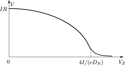
Figure 4: A schematic of the average voltage dependence on the applied magnetic field (Zeeman field $V_{Z}$) in the running state (excitation due to absorption of one quasiparticle). The blue dashed line is given by Eq. (22). The deviation from the dashed line is caused by thermal fluctuations, such as thermally activated phase slips, when the local minima of the phase potential are shallow.

The known solution for the average voltage in the running state is Tinkham (1996)

$$\left\langle V\right\rangle=R\sqrt{I^{2}-I_{c}^{2}}=R\sqrt{I^{2}-e^{2}V_{Z}^{2}D_{N}^{2}/16}\approx IR-\frac{e^{2}D_{N}^{2}V_{Z}^{2}}{32I}R,$$ (22)

which correspond to Eq. (3) in the main text for the case of $I\gg I_{c}$. One should note that now it is the average voltage in the running state, as it is varying in time, which can be easily seen from a simple model of a particle sliding down a one-dimensional washboard potential (without local minima) with friction. The higher the field is, the longer the system spends in the lower voltage regime (i.e the flatter parts of the washboard potential) with short intervals of voltages exceeding the average value (steeper parts of the phase potential). Moreover, we expect a smearing around $V_{Z}=4I/(eD_{N})$ in Eq. (22), where the voltage goes to zero according to the formula, due to thermal fluctuations (thermally activated phase slips for shallow local minima of the phase potential), see Fig 4.

As a result, in the trivial state with low magnetic fields quasiparticle poisoning would result in rare switching to the running state with a average voltage given by Eq. (22) and lasting for a short time $\tau_{r}=1/\Gamma_{r}\ll\tau_{qp}^{triv}$, where $\tau_{qp}^{triv}=1/\Gamma_{t}$ is the characteristic time between quasiparticle poisoning events (quasiparticles getting trapped in the lower ABS). However, for larger magnetic fields, $V_{Z}\gtrsim 4I/(eD_{N})$, no voltage will develop in the trivial phase.

References

- Klinovaja and Loss (2012) J. Klinovaja and D. Loss, Phys. Rev. B 86, 085408 (2012).
- San-Jose et al. (2013) P. San-Jose, J. Cayao, E. Prada, and R. Aguado, New J. Phys. 15, 075019 (2013).
- Murthy et al. (2020) C. Murthy, P. D. Kurilovich, V. D. and. Kurilovich, B. van Heck, L. I. Glazman, and C. Nayak, Phys. Rev. B. 101, 224501 (2020).
- Fu and Kane (2009) L. Fu and C. L. Kane, Phys. Rev. B 79, 161408 (2009).
- Cayao et al. (2017) J. Cayao, P. San-Jose, A. M. Black-Schaffer, R. Aguado, and E. Prada, Phys. Rev. B 96, 205425 (2017).
- Pikulin and Nazarov (2012) D. I. Pikulin and Y. V. Nazarov, Phys. Rev. B. 86, 140504(R) (2012).
- Domínguez et al. (2012) F. Domínguez, F. Hassler, and G. Platero, Phys. Rev. B. 86, 140503(R) (2012).
- Levenson-Falk et al. (2014) E. M. Levenson-Falk, F. Kos, R. Vijay, L. Glazman, and I. Siddiqi, Phys. Rev. Lett. 112, 047002 (2014).
- Tinkham (1996) M. Tinkham, in Introduction to Superconductivity (Second Edition, McGraw-Hill Book Co., 1996).