Graph-structured tensor optimization for
nonlinear density control and mean field games

Abstract

In this work we develop a numerical method for solving a type of convex graph-structured tensor optimization problems. This type of problems, which can be seen as a generalization of multi-marginal optimal transport problems with graph-structured costs, appear in many applications. In particular, we show that it can be used to model and solve nonlinear density control problems, including convex dynamic network flow problems and multi-species potential mean field games. The method is based on coordinate ascent in a Lagrangian dual, and under mild assumptions we prove that the algorithm converges globally. Moreover, under a set of stricter assumptions, the algorithm converges R-linearly. To perform the coordinate ascent steps one has to compute projections of the tensor, and doing so by brute force is in general not computationally feasible. Nevertheless, for certain graph structures we derive efficient methods for computing these projections. In particular, these graph structures are the ones that occur in convex dynamic network flow problems and multi-species potential mean field games. We also illustrate the methodology on numerical examples from these problem classes.

I Introduction

A strong trend in many research fields is the study of large-scale systems consisting of components that are subsystems with specific characteristics. Examples of such technological systems that are currently emerging include smart electric grids [farhangi2010path], and road networks with self-driving cars [meyer2014road]. There are also many such problems in biology, ecology, and social sciences, including, e.g., cell, animal, or human populations [watts1998collective]. A major challenge is to understand and control the macroscopic behavior of such complex large-scale systems.

Since the number of agents is often too large to model each agent individually, the overall system is typically viewed as a flow or density control problem. In this setting, the aggregate state information of the agents is often described by a distribution or density function, and classical problems of this form include, e.g., network flow problems. More recently, there has been a large interest in control and estimation of densities, and one key result is that certain density control problems of first-order integrators can be seen as optimal transport problems [benamou2000computational]. This correspondence can be extended to general dynamics, and thus the optimal transport problem can be interpreted as a density control problem of agents (subsystems) with general dynamics [hindawi2011mass, chen2017optimal, caluya2021wasserstein].

Even though optimal transport problems are linear programs, the number of variables is often very large and thus the problems can be computationally challenging. A computational breakthrough is the use of Sinkhorn’s method for computing an approximate solution. This builds on the insight that the entropy regularized problem can be efficiently solved using dual coordinate ascent [cuturi2013sinkhorn, peyre2019computational]. Interestingly, the entropy regularization term can also be interpreted in this setting as introducing stochasticity in the dynamics of the subsystems, and can in fact be shown to be equivalent to the Schrödinger bridge problem [leonard2012schrodinger, leonard2013schrodinger, chen2020stochastic].

Many density flow problems can be viewed as a two-marginal problem. However, many problems involve using a time grid in order to model, e.g., congestion, instantaneous costs, or observations [haasler2020optimal]. For such problems it is natural to use versions of the multi-marginal optimal transport problem, where marginals represent the distributions at different time points $j=1,\ldots,{\mathcal{T}}$. The multi-marginal optimal transport problem is an optimization problem where a nonnegative tensor is sought to minimize a linear cost subject to constraints on the marginals, where the marginals correspond to projections of the tensor on specific modes.

In this paper, we generalize the multi-marginal optimal transport problem and consider optimization problems on tensors with certain structures that appear in, e.g., density control problems and mean field games. More specifically, for such control problems with identical and indistinguishable agents, the Markov property may be used to separate the problem into ${\mathcal{T}}-1$ parts, where each part represents the evolution during time interval $[j,j+1]$ for $j=1,\ldots,{\mathcal{T}}-1$. The transition of the agents from time $j$ to time $j+1$ can thus be specified by the bimarginal projection of the tensor onto the joint two marginals $j$ and $j+1$, and thus this problem is a structured tensor problem with structure corresponding to a path graph (see, e.g., [chen2018state, elvander2020multi, haasler2021multimarginal]). However, when the agents have heterogeneous dynamics or objectives, the distribution at a given time does not contain all necessary information about the past and thus the Markov property does not hold. Nevertheless, many problems of interest can instead be modeled by introducing additional dependencies between marginals. For example, traffic flow problems with origin destination constraints can be formulated by introducing dependence between the initial and final node [haasler2020optimal], and Euler flow problems can be seen as a special case of this [benamou2015bregman]. By introducing an additional marginal representing different types of agents we can also formulate and solve multi-species dynamic flow problems and large multi-commodity problems [haasler2021scalable]. Interesting to note in this context is that the algorithms developed to solve this type of structured problems are closely related to the unified propagation and scaling algorithm for inference in graphical models [teh2002propagation].

Many of the problems in the previous paragraph can be formulated as linear optimization problems. Nevertheless, in many situations it is also natural to consider problems with convex costs, for example in potential mean field games [BenCarDiNen19], but standard convex optimization methods in general do not scale to this type of large-scale problems. The contribution of this paper is therefore to develop a theoretical framework for a type of convex structured tensor optimization problems, along with numerical solution methods and convergence results for these. We also illustrate how this type of problems can be used to model and solve, e.g., convex dynamic flow problems [ouorou2000survey], density control problems, and multi-species potential mean field games. An important observation is that the dual problem has a decomposable form, and can be efficiently solved using dual coordinate ascent [karlsson2017generalized] (cf. [peyre2019computational]). Moreover, the structure in these problems can be represented by a graph connecting the marginals, and by utilizing this graph we show how marginal and bimarginal projections of the tensor can be computed efficiently, thus alleviating the computational bottleneck of the algorithm (cf. [haasler2021scalable]).

The outline of the paper is as follows: in Section II we introduce some background material on optimal transport and convex optimization. The main results are presented in Section III, where we formulate the graph-structured tensor optimization problem of interest and present a primal-dual framework for solving it, together with a Sinkhorn-type algorithm for iteratively solving the dual problem. Conditions for convergence and R-linear convergence are also presented. Based on this, in Section IV and V we develop algorithms for solving two important types of problems: convex dynamic network flow problems and multi-species potential mean field games, respectively. This is done by casting the corresponding problem as a graph-structured tensor optimization problem and then specializing the general algorithm to the particular instance. Moreover, in each of the two sections we also present numerical examples to illustrate the use and performance of the algorithms. Finally, Section VI contains some concluding remarks. Some proofs are deferred to the appendix for improved readability. This paper builds on [ringh2021efficient], where we presented an algorithm, without proof of convergence, for the multi-species mean field game in a simplified setting (see also remark V.3).

II Background

This section presents background material, in particular on graph-structured multi-marginal optimal transport. We also introduce some concepts from convex analysis and convex optimization that are needed in this work.

II-A The graph-structured multi-marginal optimal transport problem

The optimal transport problem seeks a transport plan for how to move mass from an initial distribution to a target distribution with minimum cost. This topic has been extensively studied, see, e.g., the monograph [villani2003topics] and references therein. An extension of this problem is the multi-marginal optimal transport problem, in which a minimum-cost transport plan between several distributions is sought [ruschendorf1995optimal, gangbo1998optimal, ruschendorf2002n, pass2015multi, benamou2015bregman, nenna2016numerical, elvander2020multi]. In this work we consider the discrete case of the latter, where the marginal distributions are given by a finite set of ${\mathcal{T}}$ nonnegative vectors $\mu_{1},\ldots,\mu_{\mathcal{T}}\in{\mathbb{R}}^{N}_{+}$. The transport plan and the corresponding cost of moving mass are both represented by ${\mathcal{T}}$-mode tensors ${\bf M}\in{\mathbb{R}}^{N^{\mathcal{T}}}_{+}$ and ${\bf C}\in{\mathbb{R}}^{N^{\mathcal{T}}}$, respectively. More precisely, ${\bf M}_{i_{1}\ldots i_{\mathcal{T}}}$ and ${\bf C}_{i_{1}\ldots i_{\mathcal{T}}}$ are the transported mass and the cost of moving mass associated with the tuple $(i_{1},\ldots,i_{{\mathcal{T}}})$, respectively. The total cost of transport is therefore given by

$$\langle{\bf C},{\bf M}\rangle:=\sum_{i_{1},\ldots,i_{\mathcal{T}}}{\bf C}_{i_{1}\ldots i_{\mathcal{T}}}{\bf M}_{i_{1}\ldots i_{\mathcal{T}}}.$$

Moreover, for ${\bf M}$ to be a feasible transport plan, it must have the given distributions as its marginals. To this end, the marginal distributions of ${\bf M}$ are given by the projections $P_{j}({\bf M})\in{\mathbb{R}}^{N}_{+}$, where

$$(P_{j}({\bf M}))_{i_{j}}:=\sum_{i_{1},\ldots,i_{j-1},i_{j+1},i_{\mathcal{T}}}{\bf M}_{i_{1}\ldots i_{\mathcal{T}}},$$

and hence ${\bf M}$ is feasible if $P_{j}({\bf M})=\mu_{j}$ for $j=1,\ldots,{\mathcal{T}}$. A generalization of this optimization problem is to not necessarily impose marginal constraints on all projections $P_{j}({\bf M})$, but only for an index set $\Gamma\subset\{1,\ldots,{\mathcal{T}}\}$. The discrete multi-marginal optimal transport problem can thus be formulated as

$$\underset{{\bf M}\in{\mathbb{R}}^{N^{{\mathcal{T}}}}_{+}}{\text{minimize }} \quad\langle{\bf C},{\bf M}\rangle$$ (1a)

subject to $$\quad P_{j}({\bf M})=\mu_{j},\quad j\in\Gamma.$$ (1b)

Problem (1) is a linear program, however solving it can be computationally challenging due to the large number of variables. An approach for obtaining approximate solutions in the bimarginal case is to add a small entropy term to the cost function and solve the corresponding perturbed problem [cuturi2013sinkhorn] (see also [peyre2019computational]). This perturbed problem can be solved by using the so-called Sinkhorn iterations. The approach has been extended to the multi-marginal setting [benamou2015bregman, nenna2016numerical, elvander2020multi], however in this case it only partly alleviates the computational difficulty. More precisely, in the multi-marginal setting the entropy term is defined as

$$D({\bf M}):=\sum_{i_{1},\ldots,i_{\mathcal{T}}}\big{(}{\bf M}_{i_{1}\ldots i_{\mathcal{T}}}\log({\bf M}_{i_{1}\ldots i_{\mathcal{T}}})-{\bf M}_{i_{1}\ldots i_{\mathcal{T}}}+1\big{)},$$

and the optimal solution to the perturbed problem can be shown to take the form [benamou2015bregman, elvander2020multi]

$${\bf M}={\bf K}\odot{\bf U},$$

where ${\bf K}=\exp(-{\bf C}/\epsilon)$, $\odot$ denotes the elementwise product, and ${\bf U}$ is the rank-one tensor

$${\bf U}_{i_{1}\dots i_{\mathcal{T}}}=\prod_{j\in\Gamma}u_{j}^{(i_{j})},$$

i.e., ${\bf U}=(\otimes_{j\in\Gamma}u_{j})\otimes(\otimes_{j\in\{1,\ldots,{\mathcal{T}}\}\setminus\Gamma}{\bf 1})$, where $\otimes$ denotes the tensor product and ${\bf 1}$ denotes a vector of ones. In fact, the variables $u_{j}$ are the logarithms of the Lagrangian dual variables in a relaxation of the entropy-regularized version of (1). Moreover, the (multi-marginal) Sinkhorn iterations iteratively update $u_{j}$ to match the given marginals:

$$u_{j}\leftarrow u_{j}\odot\mu_{j}\oslash P_{j}({\bf K}\odot{\bf U}),\quad\text{ for }j\in\Gamma,$$

where $\oslash$ denotes elementwise division. However, in the multi-marginal case, computing $P_{j}({\bf K}\odot{\bf U})$ is challenging since the number of terms in the sum grows exponentially with the number of marginals, and the latter is also reflected in complexity bounds for the algorithm [lin2022complexity]. Nevertheless, in some cases when the underlying cost ${\bf C}$ is structured the projections can be computed efficiently. In particular, this is the case for certain graph-structured costs.

To this end, let ${\mathcal{G}}=({\mathcal{V}},{\mathcal{E}})$ be a connected graph with ${\mathcal{T}}=|{\mathcal{V}}|$ nodes, and consider the optimization problem

$$\underset{{\bf M}\in{\mathbb{R}}_{+}^{N^{{\mathcal{T}}}}}{\text{minimize }} \quad\langle{\bf C},{\bf M}\rangle+\epsilon D({\bf M})$$ (2a)

subject to $$\quad P_{t}({\bf M})=\mu_{t},\quad t\in\tilde{\mathcal{V}},$$ (2b)

where $\tilde{\mathcal{V}}\subset{\mathcal{V}}$ is a set of vertices. Moreover, consider cost tensor ${\bf C}$ with the structure

$${\bf C}_{i_{1}\ldots i_{\mathcal{T}}}=\sum_{(t_{1},t_{2})\in{\mathcal{E}}}C^{(t_{1},t_{2})}_{i_{t_{1}},i_{t_{2}}},$$ (3)

where $C^{(t_{1},t_{2})}\in{\mathbb{R}}^{N\times N}$, which in particular means that the linear cost term takes the form

$$\langle{\bf C},{\bf M}\rangle=\sum_{(t_{1},t_{2})\in{\mathcal{E}}}\langle C^{(t_{1},t_{2})},P_{t_{1},t_{2}}({\bf M})\rangle.$$

Here $P_{t_{1},t_{2}}({\bf M})\in{\mathbb{R}}_{+}^{N\times N}$ denotes the joint projection of the tensor ${\bf M}$ on the two marginals $t_{1}$ and $t_{2}$, given by

$$(P_{t_{1},t_{2}}({\bf M}))_{i_{t_{1}},i_{t_{2}}}:=\sum_{\{i_{1},\ldots,i_{\mathcal{T}}\}\setminus\{i_{t_{1}},i_{t_{2}}\}}{\bf M}_{i_{1}\ldots i_{\mathcal{T}}}.$$

Problem (2) with a cost tensor structured according to (3) is called a (entropy-regularized) graph-structured multi-marginal optimal transport problem [haasler2021scalable, haasler2021multimarginal, fan2022complexity]. Moreover, for many graph structures, the projections $P_{j}({\bf M})$ can be efficiently computed, see, e.g, [benamou2015bregman, haasler2020optimal, elvander2020multi, haasler2021multimarginal, haasler2021scalable, haasler2020multi, singh2020inference, altschuler2020polynomial, haasler2021control, fan2022complexity], and hence the Sinkhorn iterations can be used to efficiently solve such problems.

II-B Convex analysis and optimization

We need the following definitions and results from convex analysis and optimization. For extensive treatments of the topic, see, e.g., the monographs [rockafellar1970convex, luenberger1969optimization, bauschke2017convex]. To this end, let $f:{\mathbb{R}}^{n}\to{\bar{{\mathbb{R}}}}:={\mathbb{R}}\cup\{\pm\infty\}$ be an extended real-valued function. The epigraph of $f$ is defined as $\text{epi}(f):=\{(x,\eta)\in{\mathbb{R}}^{n}\times{\mathbb{R}}\mid f(x)\leq\eta\}$, and $f$ is called convex if $\text{epi}(f)\subset{\mathbb{R}}^{n+1}$ is a convex set. A function $f$ is lower-semicontinuous if and only if $\text{epi}(f)$ is closed [rockafellar1970convex, Thm. 7.1]. The effective domain of $f$ is defined as $\text{dom}(f):=\{x\in{\mathbb{R}}^{n}\mid f(x)<\infty\}$, and $f$ is called proper if $f(x)>-\infty$ for all $x\in{\mathbb{R}}^{n}$ and $\text{dom}(f)\neq\emptyset$. A convex set $C$ is called polyhedral if it can be written as the intersection of a finite number of closed half spaces. A convex function $f$ is called polyhedral if $\text{epi}(f)$ is polyhedral. The Fenchel conjugate of a function $f$ is defined as $f^{*}(x^{*}):=\sup_{x}\langle x^{*},x\rangle-f(x)$. A convex, proper, lower-semicontinuous function $f$ is called co-finite if $\text{epi}(f)$ contains no non-vertical half-lines, which is equivalent to that $f^{*}$ is finite everywhere, i.e., that $\text{dom}(f^{*})={\mathbb{R}}^{n}$, [rockafellar1970convex, Cor. 13.3.1].

The subdifferential of a function $f$ in a point $x$ is the set $\partial f(x):=\{u\in{\mathbb{R}}^{n}\mid\langle y-x,u\rangle+f(x)\leq f(y)\;\forall\,y\in{\mathbb{R}}^{n}\}$, and if $f$ is proper, convex, and differentiable in $x$ with gradient $\nabla f(x)$, then $\partial f(x)=\{\nabla f(x)\}$ [bauschke2017convex, Prop. 17.31]. A convex, proper, lower-semicontinuous function $f$ is called essentially smooth if i) it is differentiable on $\text{int}(\text{dom}(f))$, i.e., on the interior of the effective domain, and ii) $\lim_{\ell\to\infty}\|\nabla f(x_{\ell})\|\to\infty$ for any sequence $\{x_{\ell}\}_{\ell}\subset\text{int}(\text{dom}(f))$ that either converges to the boundary of $\text{int}(\text{dom}(f))$ or is such that $\|x_{\ell}\|\to\infty$. Finally, an operator $A:{\mathbb{R}}^{n}\to{\mathbb{R}}^{n}$ is called strongly monotone if there exists a $\gamma>0$ such that $\langle Ax-Ay,x-y\rangle\geq\gamma\|x-y\|^{2}$ for all $x,y\in{\mathbb{R}}^{n}$.

III Convex graph-structured tensor optimization

In this work, we consider a family of optimization problems that generalizes problems of the form (2). To this end, let ${\mathcal{G}}=({\mathcal{V}},{\mathcal{E}})$ be a connected graph with ${\mathcal{T}}=|{\mathcal{V}}|$ nodes, and let ${\bf C}\in{\bar{{\mathbb{R}}}}^{N^{\mathcal{T}}}$ be a cost tensor that takes the form (3). The convex graph-structured tensor optimization problems of interest are problems of the form

$$\underset{{\bf M}\in{\mathbb{R}}_{+}^{N^{{\mathcal{T}}}}}{\text{minimize }} \quad\langle{\bf C},{\bf M}\rangle+\epsilon D({\bf M})+\sum_{t\in{\mathcal{V}}}g^{(t)}(P_{t}({\bf M}))$$

$$\quad+\sum_{(t_{1},t_{2})\in{\mathcal{E}}}f^{(t_{1},t_{2})}(P_{t_{1},t_{2}}({\bf M})),$$ (4)

where $g^{(t)}$ and $f^{(t_{1},t_{2})}$ are proper, convex, and lower-semicontinuous functionals; further assumptions on these functionals will be imposed where needed. The reason for our interest in problems of the form (4) is that a number of different applications can be modeled as such problems. In particular, this is true for convex dynamic network flow problems, and potential multi-species mean field games. These two applications are studied in detail in Sections IV and V, respectively.

Remark III.1.

To see that problems of the form (4) is a generalization of the graph-structured optimal transport problem (2), let $I_{A}(\cdot)$ denote the indicator function on the set $A$, i.e., the function

$$I_{A}(x):=\begin{cases}0,&\text{if }x\in A\\ \infty,&\text{else,}\end{cases}$$

and note that this function is proper, convex, and lower-semicontinuous if and only if $A$ is a nonempty, closed, convex set. Now, (2) is recovered from (4) by taking $g^{(t)}(P_{t}({\bf M}))=I_{\{\mu_{t}\}}(P_{t}({\bf M}))$ for $t\in\tilde{{\mathcal{V}}}$ and $g^{(t)}(P_{t}({\bf M}))\equiv 0$ otherwise, and $f^{(t_{1},t_{2})}(P_{t_{1},t_{2}}({\bf M}))\equiv 0$ for all $(t_{1},t_{2})\in{\mathcal{E}}$. Another particular case of interest is a version of (2), but where some of the equality constraints are replaced by inequality constraints, cf. [haasler2021scalable].

Remark III.2.

In problem (4) the functions $f^{(t_{1},t_{2})}$ and the tensor ${\bf C}$ are defined on the same set of edges ${\mathcal{E}}$. This is done for convenience of notation, and is not a restrictive assumption. To see this, note that it is possible to define certain functions $f^{(t_{1},t_{2})}$ to be the zero function, or to take certain matrices $C^{(t_{1},t_{2})}$ in the decomposition (3) to be the zero-matrix.

Note that (4) is typically a large-scale problem, where the full set of variables may neither be stored nor manipulated directly. Therefore one must utilize the problem structure in order to compute the solution. In this section, we develop a method for such problems, based on generalized Sinkhorn iterations. This methodology for handling the problem builds on deriving the Lagrangian dual of an optimization problem that is equivalent to (4), and solving this dual using coordinate ascent. As we will see, the method exploits the graph structure and the algorithm is efficient when the graph is simple, i.e., the tree-width is low (cf. [haasler2021scalable, fan2022complexity, haasler2020multi]), and when the functionals $g^{(t)}$ and $f^{(t_{1},t_{2})}$ are in some sense simple.

III-A An equivalent problem and existence of solution

We first introduce and analyze a problem that is equivalent to (4), and give conditions under which the latter has an optimal solution. To this end, introducing the variables $\mu_{t}$, $t\in{\mathcal{V}}$, and $R_{t_{1},t_{2}}$, $(t_{1},t_{2})\in{\mathcal{E}}$, problem (4) can be rewritten as

$$\underset{\begin{subarray}{c}{\bf M}\in{\mathbb{R}}_{+}^{N^{{\mathcal{T}}}},\;\mu_{t}\in{\mathbb{R}}^{N},\;t\in{\mathcal{V}}\\ R_{t_{1},t_{2}}\in{\mathbb{R}}^{N\times N},\;(t_{1},t_{2})\in{\mathcal{E}}\end{subarray}}{\text{minimize }} \langle{\bf C},{\bf M}\rangle+\epsilon D({\bf M})+\sum_{t\in{\mathcal{V}}}g^{(t)}(\mu_{t})$$

$$\;+\sum_{(t_{1},t_{2})\in{\mathcal{E}}}f^{(t_{1},t_{2})}(R_{t_{1},t_{2}})$$ (5a)

subject to $$\;P_{t}({\bf M})=\mu_{t},\;t\in{\mathcal{V}}$$ (5b)

$$\;P_{t_{1},t_{2}}({\bf M})=R_{t_{1},t_{2}},\;(t_{1},t_{2})\in{\mathcal{E}}.$$ (5c)

In order for this to be a well-posed problem, we impose the following assumptions on the functionals involved.

Assumption A.

Assume that all elements of ${\bf C}$ are strictly larger than $-\infty$, and that $g^{(t)}$, $t\in{\mathcal{V}}$, and $f^{(t_{1},t_{2})}$, $(t_{1},t_{2})\in{\mathcal{E}}$, are all proper, convex, and lower-semicontinuous, Moreover, assume that there exists a feasible point to (5) with finite objective function value, i.e., a nonnegative tensor ${\bf M}$ such that $\langle{\bf C},{\bf M}\rangle<\infty$, and with marginals and bimarginals as in (5b)-(5c), respectively, such that

$$g^{(t)}(\mu_{t})<\infty,\quad\text{ for all }t\in{\mathcal{V}},$$

$$f^{(t_{1},t_{2})}(R_{t_{1},t_{2}})<\infty,\quad\text{ for all }(t_{1},t_{2})\in{\mathcal{E}}.$$

In fact, this assumption ensures that (5) has an optimal solution, as stated in the following lemma.

Lemma III.3.

If Assumption A holds, then there exists a unique optimal solution to problem (5).

Proof.

See Appendix -A. ∎

Remark III.4.

A necessary condition for Assumption A to hold is that there exist vectors $\mu_{t}\in{\mathbb{R}}_{+}^{N}\cap\text{dom}(g^{(t)})$, for all $t\in{\mathcal{V}}$, matrices $R_{t_{1},t_{2}}\in{\mathbb{R}}_{+}^{N\times N}\cap\text{dom}(f^{(t_{1},t_{2})})$, for all $(t_{1},t_{2})\in{\mathcal{E}}$, and a constant $\gamma\geq 0$ such that

$$\mu_{t}^{T}{\bf 1}=\gamma,\quad\text{ for all }t\in{\mathcal{V}}$$

$$R_{t_{1},t_{2}}{\bf 1}=\mu_{t_{1}},\;R_{t_{1},t_{2}}^{T}{\bf 1}=\mu_{t_{2}},\quad\text{ for all }(t_{1},t_{2})\in{\mathcal{E}},$$

$$\langle C^{(t_{1},t_{2})},R_{t_{1},t_{2}}\rangle<\infty,\quad\text{ for all }(t_{1},t_{2})\in{\mathcal{E}}.$$

However, unless the graph $({\mathcal{V}},{\mathcal{E}})$ is a tree, this is not a sufficient condition for the existence of a tensor that fulfills Assumption A. More precisely, the existence of marginals and bimarginals that are consistent with each other does, in general, not guarantee that there exists a tensor that matches the marginals and bimarginals. A counterexample can be found in [haasler2021multimarginal, Rem. 3].

III-B Form of the optimal solution and Lagrangian dual

Next, we derive the Lagrangian dual of (5) and show that there is no duality gap between the primal and the dual problem.

Theorem III.5.

A Lagrangian dual of (5) is, up to a constant, given by

$$\sup_{\begin{subarray}{c}\lambda_{t}\in{\mathbb{R}}^{N},\;t\in{\mathcal{V}}\\ \Lambda_{t_{1},t_{2}}\in{\mathbb{R}}^{N\times N},\;(t_{1},t_{2})\in{\mathcal{E}}\end{subarray}} \quad-\epsilon\langle{\bf K},{\bf U}\rangle-\sum_{t\in{\mathcal{V}}}(g^{(t)})^{*}(-\lambda_{t})$$

$$\quad-\sum_{(t_{1},t_{2})\in{\mathcal{E}}}(f^{(t_{1},t_{2})})^{*}(-\Lambda_{t_{1},t_{2}}),$$ (6)

where ${\bf K}$ and ${\bf U}$ are given by

$${\bf K}_{i_{1}\ldots i_{{\mathcal{T}}}} =\exp(-{\bf C}_{i_{1}\ldots i_{{\mathcal{T}}}}/\epsilon),$$ (7a)

$${\bf U}_{i_{1}\ldots i_{{\mathcal{T}}}} =\prod_{t\in{\mathcal{V}}}u_{t}^{(i_{t})}\prod_{(t_{1},t_{2})\in{\mathcal{E}}}U_{t_{1},t_{2}}^{(i_{t_{1}},i_{t_{2}})}$$

$$=\prod_{t\in{\mathcal{V}}}\exp\left(\lambda_{t}^{(i_{t})}/\epsilon\right)\prod_{(t_{1},t_{2})\in{\mathcal{E}}}\exp\left(\Lambda_{t_{1},t_{2}}^{(i_{t_{1}},i_{t_{2}})}/\epsilon\right).$$ (7b)

Moreover, under Assumption A, the minimum in (5) equals the supremum in (6) (up to the discarded constant). Finally, if the dual (6) has an optimal solution, then the optimal solution to the primal problem takes the form ${\bf M}^{\star}={\bf K}\odot{\bf U}^{\star}$, where ${\bf U}^{\star}$ is obtained via (7b) from an optimal solution to (6).

Proof.

Relaxing each constraint (5b) and (5c) with a multiplier $\lambda_{t}\in{\mathbb{R}}^{N}$ and $\Lambda_{t_{1},t_{2}}\in{\mathbb{R}}^{N\times N}$, respectively, we get the Lagrangian

$$L({\bf M},\mu,R,\lambda,\Lambda):=\langle{\bf C},{\bf M}\rangle+\epsilon D({\bf M})+\sum_{t\in{\mathcal{V}}}g^{(t)}(\mu_{t})$$

$$\quad+\sum_{(t_{1},t_{2})\in{\mathcal{E}}}f^{(t_{1},t_{2})}(R_{t_{1},t_{2}})+\sum_{t\in{\mathcal{V}}}\lambda_{t}^{T}(\mu_{t}-P_{t}({\bf M}))$$

$$\quad+\sum_{(t_{1},t_{2})\in{\mathcal{E}}}\text{tr}[\Lambda_{t_{1},t_{2}}^{T}(R_{t_{1},t_{2}}-P_{t_{1},t_{2}}({\bf M}))],$$ (8)

where $\mu$ denote $(\mu_{t})_{t\in{\mathcal{V}}}$, and similar for all other variables. The dual function is given by $\inf L$ over ${\bf M}$, $\mu$, and $R$, but the Lagrangian decouples over ${\bf M}$, $\mu_{t}$, and $R_{t_{1},t_{2}}$. For the inf over $\mu_{t}$ we have that

$$\inf_{\mu_{t}}\lambda_{t}^{T}\mu_{t}+g^{(t)}\!(\mu_{t})\!=\!-\!\sup_{\mu_{t}}(-\!\lambda_{t})^{T}\!\mu_{t}-g^{(t)}\!(\mu_{t})\!=\!-(g^{(t)})^{*}(-\!\lambda_{t})$$

where $\mbox{}^{*}$ denotes the Fenchel conjugate; and analogous result follows for $f^{(t_{1},t_{2})}$ and the inf over $R_{t_{1},t_{2}}$. This means that

$$\inf_{{\bf M}\geq 0,\mu,R}L({\bf M},\mu,R,\lambda,\Lambda)=\inf_{{\bf M}\geq 0}\mathcal{L}({\bf M},\lambda,\Lambda)$$

$$\quad-\sum_{t\in{\mathcal{V}}}(g^{(t)})^{*}(-\lambda_{t})-\sum_{(t_{1},t_{2})\in{\mathcal{E}}}(f^{(t_{1},t_{2})})^{*}(-\Lambda_{t_{1},t_{2}})$$ (9)

where $\mathcal{L}({\bf M},\lambda,\Lambda)$ is defined as

$$\langle{\bf C},{\bf M}\rangle+\epsilon D({\bf M})-\sum_{t\in{\mathcal{V}}}\lambda_{t}^{T}P_{t}({\bf M})-\sum_{(t_{1},t_{2})\in{\mathcal{E}}}\text{tr}[\Lambda_{t_{1},t_{2}}^{T}P_{t_{1},t_{2}}({\bf M})].$$

Now, noticing that

$$\lambda_{t}^{T}P_{t}({\bf M})=\sum_{i_{t}=1}^{N}\lambda_{t}^{(i_{t})}\!\!\!\!\!\sum_{i_{1},\ldots,i_{{\mathcal{T}}}\setminus\{i_{t}\}}\!\!\!{\bf M}_{i_{1}\ldots i_{{\mathcal{T}}}}=\!\!\!\sum_{i_{1},\ldots,i_{{\mathcal{T}}}}\!\!\!\lambda_{t}^{(i_{t})}{\bf M}_{i_{1}\ldots i_{{\mathcal{T}}}},$$

$$\text{tr}[\Lambda_{t_{1},t_{2}}^{T}P_{t_{1},t_{2}}({\bf M})]=\sum_{i_{1},\ldots,i_{{\mathcal{T}}}}\Lambda_{t_{1},t_{2}}^{(i_{t_{1}},i_{t_{2}})}{\bf M}_{i_{1}\ldots i_{{\mathcal{T}}}},$$

$\mathcal{L}({\bf M},\lambda,\Lambda)$ decouples over the elements of the tensor. Therefore, the inf in each element is either attained in $0$, or found by setting the first variation to $0$. If ${\bf C}_{i_{1}\ldots i_{{\mathcal{T}}}}=\infty$, then the trivial case ${\bf M}_{i_{1}\ldots i_{{\mathcal{T}}}}=0$ holds. Otherwise, setting the first variation equal to $0$ gives

$$0={\bf C}_{i_{1}\ldots i_{{\mathcal{T}}}}+\epsilon\log({\bf M}_{i_{1}\ldots i_{{\mathcal{T}}}})-\sum_{t\in{\mathcal{V}}}\lambda_{t}^{(i_{t})}-\!\!\sum_{(t_{1},t_{2})\in{\mathcal{E}}}\Lambda_{t_{1},t_{2}}^{(i_{t_{1}},i_{t_{2}})}$$

from which it can be seen that the optimum is such that ${\bf M}_{i_{1}\ldots i_{{\mathcal{T}}}}>0$. Moreover, solving for ${\bf M}_{i_{1}\ldots i_{{\mathcal{T}}}}$ gives that ${\bf M}={\bf K}\odot{\bf U}$, where ${\bf K}$ and ${\bf U}$ are given in (7). Note that this form for ${\bf M}$ also holds for the elements of ${\bf C}$ that are infinite. Plugging this back into $\mathcal{L}({\bf M},\lambda,\Lambda)$ we get that $\inf_{{\bf M}\geq 0}\mathcal{L}({\bf M},\lambda,\Lambda)=-\epsilon\langle{\bf K},{\bf U}\rangle+N^{\mathcal{T}}\epsilon$, which, after removing the constant, together with (9) gives the dual problem (6).

Finally, for improved readability the detailed proof of that there is no duality gap is deferred to Lemma .2 in Appendix -A. ∎

By using the change of variables implicit in (7b), problem (6) can be expressed equivalently as

$$\underset{\begin{subarray}{c}u_{t}\in{\mathbb{R}}^{N}_{+},\;t\in{\mathcal{V}}\\ U_{t_{1},t_{2}}\in{\mathbb{R}}^{N\times N}_{+},\;(t_{1},t_{2})\in{\mathcal{E}}\end{subarray}}{\text{sup }} -\epsilon\langle{\bf K},{\bf U}\rangle-\sum_{t\in{\mathcal{V}}}(g^{(t)})^{*}\big{(}-\epsilon\log(u_{t})\big{)}$$

$$\!\!\!\!\!\!\!\!-\sum_{(t_{1},t_{2})\in{\mathcal{E}}}(f^{(t_{1},t_{2})})^{*}\big{(}-\epsilon\log(U_{t_{1},t_{2}})\big{)}.$$ (10)

Moreover, under a Slater-type condition of for the primal problem, i.e., that the relative interior (denoted ri) of the effective domains of the cost functions in (4) have a nonempty intersection, we have that the suprema in (6) and (10) are attained.

Assumption B.

Assume that there exists an ${\bf M}>0$ such that $\langle{\bf C},{\bf M}\rangle<\infty$, and with marginals and bimarginals $(\mu_{t})_{t\in{\mathcal{V}}}$ and $(R_{t_{1},t_{2}})_{(t_{1},t_{2})\in{\mathcal{E}}}$ satisfying (5b) and (5c), respectively, so that

• for all $g^{(t)}$ and $f^{(t_{1},t_{2})}$ that are polyhedral, $\mu_{t}\in\text{dom}(g^{(t)})$ and $R_{t_{1},t_{2}}\in\text{dom}(f^{(t_{1},t_{2})})$,

• for all $g^{(t)}$ and $f^{(t_{1},t_{2})}$ that are not polyhedral, $\mu_{t}\in\text{ri}(\text{dom}(g^{(t)}))$ and $R_{t_{1},t_{2}}\in\text{ri}(\text{dom}(f^{(t_{1},t_{2})}))$.

Corollary III.6.

Given Assumption B the conclusions of Theorem III.5 holds, with the addition that the dual (6) is guaranteed to have a nonempty set of optimal solutions.

Proof.

The result follows from [rockafellar1970convex, Ch. 29 and 30]. ∎

Nevertheless, even if the Slater-type condition in Assumption B is not fulfilled, the form ${\bf M}={\bf K}\odot{\bf U}$ will be important in deriving a convergent algorithm for solving (5).

Remark III.7.

For the unregularized problem, i.e., problem (4) without the term $\epsilon D({\bf M})$, the dual can be obtained by a slight modification of the above argument. More precisely, it is given by

$$\sup_{\begin{subarray}{c}\lambda_{t}\in{\mathbb{R}}^{N},\;t\in{\mathcal{V}}\\ \Lambda_{t_{1},t_{2}}\in{\mathbb{R}}^{N\times N},\;(t_{1},t_{2})\in{\mathcal{E}}\end{subarray}} -\sum_{t\in{\mathcal{V}}}(g^{(t)})^{*}(-\lambda_{t})$$ (11)

$$-\sum_{(t_{1},t_{2})\in{\mathcal{E}}}(f^{(t_{1},t_{2})})^{*}(-\Lambda_{t_{1},t_{2}})$$

subject to $$\sum_{t\in{\mathcal{V}}}\lambda_{t}^{(i_{t})}+\sum_{(t_{1},t_{2})\in{\mathcal{E}}}\Lambda_{t_{1},t_{2}}^{(i_{t_{1}},i_{t_{2}})}\leq{\bf C}_{i_{1}\ldots i_{\mathcal{T}}}.$$

In fact, the term $-\epsilon\langle{\bf K},{\bf U}\rangle$ in (6) can be interpreted as a barrier term for the constraint in (11) in the sense that when $\epsilon\to 0$ then the term $-\epsilon\langle{\bf K},{\bf U}\rangle\to-\infty$ if the constraint in (11) is not fulfilled. Nevertheless, for the unregularized problem one need to impose further assumptions in order to guarantee the existence of an optimal solution. To see this, note that for a problem instance where $g^{(t)}(\mu_{t})\equiv 0$, $t\in{\mathcal{V}}$, $f^{(t_{1},t_{2})}(R_{t_{1},t_{2}})\equiv 0$, $(t_{1},t_{2})\in{\mathcal{E}}$, and where ${\bf C}$ has at least one element which is negative, the primal problem is unbounded from below.

III-C Coordinate ascent iterations for solving the dual problem

In this section we derive an efficient solution method for (5), based on performing coordinate ascent in the dual problem (6) (or, equivalently, in (10)). To this end, let $\phi((\lambda_{t})_{t\in{\mathcal{V}}},(\Lambda_{t_{1},t_{2}})_{(t_{1},t_{2})\in{\mathcal{E}}})$ denote the objective function in the dual problem (6). Given an iterate $((\lambda_{t}^{k})_{t\in{\mathcal{V}}},(\Lambda_{t_{1},t_{2}}^{k})_{(t_{1},t_{2})\in{\mathcal{E}}})$, in a coordinate ascent step we cyclically select an element $j\in{\mathcal{V}}$ or $(j_{1},j_{2})\in{\mathcal{E}}$ and compute an update to the corresponding variable by taking $\lambda_{j}^{k+1}$ to be in

$$\operatorname*{arg\,max}_{\lambda_{j}\in{\mathbb{R}}^{N}}\quad\phi(\lambda_{j},(\lambda_{t}^{k})_{t\in{\mathcal{V}}\setminus\{j\}},(\Lambda_{t_{1},t_{2}}^{k})_{(t_{1},t_{2})\in{\mathcal{E}}}),$$ (12a)

or $$\Lambda_{j_{1},j_{2}}^{k+1}$$ to be in

$$\operatorname*{arg\,max}_{\Lambda_{j_{1},j_{2}}\in{\mathbb{R}}^{N\times N}}\phi(\Lambda_{j_{1},j_{2}},(\lambda_{t}^{k})_{t\in{\mathcal{V}}},(\Lambda_{t_{1},t_{2}}^{k})_{(t_{1},t_{2})\in{\mathcal{E}}\setminus\{(j_{1},j_{2})\}}),$$ (12b)

respectively, while taking $\lambda_{t}^{k+1}=\lambda_{t}^{k}$ and $\Lambda_{t_{1},t_{2}}^{k+1}=\Lambda_{t_{1},t_{2}}^{k}$ for all other elements. In order for this to be a well-defined algorithm, we need that the set of maximizing arguments in (12) is always nonempty. To guarantee this, we impose the following assumption (which is milder than Assumption B).

Assumption C.

Assume that ${\bf C}<\infty$ and that for each index $j\in{\mathcal{V}}$ there exists a $\mu_{j}>0$ so that

• if $g^{(j)}$ is polyhedral, then $\mu_{j}\in\text{dom}(g^{(j)})$,

• if $g^{(j)}$ is not polyhedral, then $\mu_{j}\in\text{ri}(\text{dom}(g^{(j)}))$,

and analogously for each index $(j_{1},j_{2})\in{\mathcal{E}}$, $R_{j_{1},j_{2}}$, and $f^{(j_{1},j_{2})}$.

Lemma III.8.

Under Assumptions A and C, the subproblems in (12) always have a nonempty set of maximizers.

Proof.

To prove the lemma, we restrict our attention to one subproblem of the form (12a); for subproblems of the form (12b) it follows analogously. Now, note that problem (12a) can be see as the Lagrangian dual of the primal problem

$$\underset{{\bf M}\in{\mathbb{R}}_{+}^{N^{{\mathcal{T}}}},\;\mu_{j}\in{\mathbb{R}}^{N}}{\text{minimize }} \;\langle{\bf C},{\bf M}\rangle+\epsilon D({\bf M})+g^{(j)}(\mu_{j})-\!\!\!\sum_{t\in{\mathcal{V}}\setminus\{j\}}\!\!(\lambda_{t}^{k})^{T}P_{t}({\bf M})$$

$$\quad-\sum_{(t_{1},t_{2})\in{\mathcal{E}}}\text{tr}[(\Lambda_{t_{1},t_{2}}^{k})^{T}P_{t_{1},t_{2}}({\bf M})]$$

subject to $$\;P_{j}({\bf M})=\mu_{j}.$$

Moreover, using Assumption C we have that $\mu_{j}>0$ and ${\bf M}=\mu_{j}\otimes(\otimes_{t\in{\mathcal{V}}\setminus\{j\}}{\bf 1})>0$ is a point fulfilling Slater’s condition for the above problem. Therefore, following [rockafellar1970convex, Ch. 29 and 30] we have that strong duality holds between these two problems, and in particular that the dual (12a) has a nonempty set of maximizers (cf. [tseng1993dual, Lem. 3.1]). ∎

By the above lemma, the coordinate ascent steps in (12) are well-defined. Moreover, since each problem is concave and unconstrained, the optimal solution is where the subgradient is zero. To compute the subgradients, first note that

$$P_{j}({\bf K}\odot{\bf U})\oslash u_{j}=\!\!\sum_{i_{1},\ldots,i_{{\mathcal{T}}}\setminus i_{j}}\!\!{\bf K}_{i_{1}\ldots i_{\mathcal{T}}}\!\!\prod_{t\in{\mathcal{V}}\setminus\{j\}}\!\!u_{t}^{(i_{t})}\!\!\prod_{(t_{1},t_{2})\in{\mathcal{E}}}\!\!U_{t_{1},t_{2}}^{(i_{t_{1}},i_{t_{2}})}$$

is a well-defined vector which is independent of $u_{j}$. We therefore define

$$w_{j}:=P_{j}({\bf K}\odot{\bf U})\oslash u_{j},$$ (13a)

and note that this means that $$P_{j}({\bf K}\odot{\bf U})=u_{j}\odot w_{j}$$. Analogously, we also define

$$W_{j_{1},j_{2}}:=P_{j_{1},j_{2}}({\bf K}\odot{\bf U})\oslash U_{j_{1},j_{2}},$$ (13b)

which in the same way is a well-defined matrix, independent of $U_{j_{1},j_{2}}$, and hence $P_{j_{1},j_{2}}({\bf K}\odot{\bf U})=U_{j_{1},j_{2}}\odot W_{j_{1},j_{2}}$.

Next, note that

$$\frac{\partial}{\partial\lambda_{j}^{(i_{j})}}\langle{\bf K},{\bf U}\rangle=-\exp\left(\lambda_{j}^{(i_{j})}/\epsilon\right)w_{j}^{(i_{j})}=-u_{j}^{(i_{j})}w_{j}^{(i_{j})}$$

with ${\bf K}$ and ${\bf U}$ given as in (7) and $w_{j}$ as in (13a). Thus, in each update of the variable $\lambda_{j}$ one has to solve the inclusion problem

$$0\in\partial_{\lambda_{j}}\phi\!=\!-\exp\left(\lambda_{j}/\epsilon\right)\odot w_{j}+\partial(g^{(j)})^{*}(-\lambda_{j}),$$ (14a)

where $$\partial_{\lambda_{j}} \lambda_{j} \Lambda_{j_{1},j_{2}}$$ denotes the subdifferential with respect to . By an analogous derivation, in each update of the variable one has to solve the inclusion problem

$$0\in\partial_{\Lambda_{j_{1},j_{2}}}\phi= -\exp\left(\Lambda_{j_{1},j_{2}}/\epsilon\right)\odot W_{j_{1},j_{2}}$$

$$+\partial(f^{(j_{1},j_{2})})^{*}(-\Lambda_{j_{1},j_{2}}).$$ (14b)

These inclusions, and hence the updates, can be reformulated in terms of the transformed dual variables $u_{j}$ and $U_{j_{1},j_{2}}$, in which case they read

$$0\in-u_{j}\odot w_{j}+\partial(g^{(j)})^{*}\big{(}-\epsilon\log(u_{j})\big{)},$$ (15a)

$$0\in-U_{j_{1},j_{2}}\odot W_{j_{1},j_{2}}+\partial(f^{(j_{1},j_{2})})^{*}\big{(}-\!\epsilon\log(U_{j_{1},j_{2}})\big{)}.$$ (15b)

This is summarized in Algorithm 1. However, note that directly computing $w_{j}$ and $W_{j_{1},j_{2}}$ needed in (15) by brute-force is computationally demanding, and effectively numerically infeasible for large-scale problems. Therefore, from this perspective Algorithm 1 is an “abstract algorithm”. Nevertheless, for many graph structures it is possible to compute the projections efficiently by sequentially eliminating the modes of the tensor, see [benamou2015bregman, haasler2020optimal, elvander2020multi, haasler2021multimarginal, haasler2021scalable, haasler2020multi, haasler2021control, singh2020inference, altschuler2020polynomial]. In fact, storing and using intermediate results of eliminated modes, the procedure can also be understood as a message-passing scheme [haasler2020multi]. Moreover, the examples of applications presented in Sections IV and V can be effectively solved in this way, and for each of these we present an implementable algorithm (see Algorithms 2 and 3). Finally, under relatively mild assumptions, Algorithm 1 is convergent in the following sense.

1:  Give: graph ${\mathcal{G}}=({\mathcal{V}},{\mathcal{E}})$, cost tensor ${\bf C}$ that decouples according to ${\mathcal{G}}$, functions $(g^{(t)})^{*}$, for $t\in{\mathcal{V}}$, and $(f^{(t_{1},t_{2})})^{*}$, for $(t_{1},t_{2})\in{\mathcal{E}}$, nonnegative initial guesses $(u_{t}^{0})_{t\in{\mathcal{V}}}$ and $(U_{t_{1},t_{2}}^{0})_{(t_{1},t_{2})\in{\mathcal{E}}}$.

2:  $k=0$

3:  while Not converged do

4:     $k=k+1$

5:     for $j\in{\mathcal{V}}$ and $(j_{1},j_{2})\in{\mathcal{E}}$ do

6:        Update $u_{j}^{k}$ by solving (15a) with $w_{j}$ as in (13a).

7:        Update $U_{j_{1},j_{2}}^{k}$ by solving (15b) with $W_{j_{1},j_{2}}$ as in (13b).

8:     end for

9:  end while

10:  return  $(u_{t}^{k})_{t\in{\mathcal{V}}}$ and $(U_{t_{1},t_{2}}^{k})_{(t_{1},t_{2})\in{\mathcal{E}}}$.

Algorithm 1 Generalized Sinkhorn method for solving (5).

Theorem III.9.

Given that Assumptions A and C hold, and assume further that

1. $g^{(t)}$, $t\in{\mathcal{V}}$, and $f^{(t_{1},t_{2})}$, $(t_{1},t_{2})\in{\mathcal{E}}$, are all continuous on $\text{dom}(g^{(t)})$ and $\text{dom}(f^{(t_{1},t_{2})})$, respectively,

2. for all $g^{(t)}$, $t\in{\mathcal{V}}$, and $f^{(t_{1},t_{2})}$, $(t_{1},t_{2})\in{\mathcal{E}}$, that are not polyhedral, the feasible point in Assumption A is such that $\mu_{t}\in\text{ri}(\text{dom}(g^{(t)}))$ and $R_{t_{1},t_{2}}\in\text{ri}(\text{dom}(f^{(t_{1},t_{2})}))$, respectively.

Let $(u_{t}^{k})_{t\in{\mathcal{V}}}$ and $(U_{t_{1},t_{2}}^{k})_{(t_{1},t_{2})\in{\mathcal{E}}}$ be the iterates of Algorithm 1 at iteration $k$, and let ${\bf U}^{k}$ be the corresponding tensor as in (7b). Moreover, let ${\bf M}^{k}={\bf K}\odot{\bf U}^{k}$. Then $({\bf M}^{k})_{k}$ is a bounded sequence that converges to the optimal solution to (5). Furthermore, if the set of optimal solutions to (6) is nonempty and bounded, then $((u_{t}^{k})_{t\in{\mathcal{V}}},(U_{t_{1},t_{2}}^{k})_{(t_{1},t_{2})\in{\mathcal{E}}})_{k}$ is a bounded sequence and every cluster point is an optimal solution to (10).

Proof.

To prove the theorem, we define

$$h({\bf M}):=\langle{\bf C},{\bf M}\rangle+\epsilon D({\bf M}).$$

This is a strictly convex function, since the entropy term is strictly convex [bauschke2017convex, Ex. 9.35]. Moreover $\text{dom}(h)={\mathbb{R}}_{+}^{N^{\mathcal{T}}}$, and hence polyhedral. Next, the Fenchel conjugate of $h$ can be obtained by using [bauschke2017convex, Ex. 13.2] and [bauschke2017convex, Prop 13.23], which gives

$$h^{*}({\bf T}) =-\epsilon\sum_{i_{1}\ldots i_{\mathcal{T}}}\exp(({\bf T}_{i_{1}\ldots i_{\mathcal{T}}}-{\bf C}_{i_{1}\ldots i_{\mathcal{T}}})/\epsilon)-1$$

$$=-\epsilon\langle{\bf K},\exp({\bf T}/\epsilon)\rangle+n^{\mathcal{T}}\epsilon,$$

(compare with the expression $\inf_{{\bf M}}\mathcal{L}({\bf M},\lambda,\Lambda)=-\epsilon\langle{\bf K},{\bf U}\rangle+N^{\mathcal{T}}\epsilon$ in the proof of Theorem III.5). Hence, $h$ is co-finite. Therefore, following along the lines of [tseng1993dual, Sec. 6], we have that $({\bf M}^{k})_{k}$ is a bounded sequence and that every cluster point is an optimal solution to (5). In particular, [tseng1993dual, Thm. 3.1] imposes some slightly stronger assumptions, but it is readily checked in all places where these stronger assumptions are invoked that the same conclusions hold true in this particular case under the weaker assumptions. For brevity, we omit the details.

Next, since $({\bf M}^{k})_{k}$ is a bounded sequence and every cluster point is optimal to (5), by the uniqueness of the optimal solution ${\bf M}^{\star}$ the sequence must converge to it. To see this, for $\delta>0$ let $B_{\delta}({\bf M}^{\star})$ denote a ball of radius $\delta$ around ${\bf M}^{\star}$. If there is an infinite number of points of $({\bf M}^{k})_{k}$ outside of $B_{\delta}({\bf M}^{\star})$, since the corresponding subsequence is also bounded there is a converging subsubsequence, i.e., the subsubsequence has a cluster point; call this cluster point ${\bf M}^{\infty}$. Since this is also a cluster point of the original sequence, we must have ${\bf M}^{\infty}={\bf M}^{\star}$, but we must also have that ${\bf M}^{\infty}\not\in B_{\delta}({\bf M}^{\star})$, which is a contradiction. Therefore, for every $\delta>0$ there can only be a finite number of points in the sequence $({\bf M}^{k})_{k}$ that do not belong to $B_{\delta}({\bf M}^{\star})$, and hence the entire sequence converges to ${\bf M}^{\star}$.

Finally, the last statement of the theorem follows similarly from [tseng1993dual, Thm. 3.1(b)]. ∎

The above theorem guarantees convergence, but does not guarantee how fast the iterates converge. In particular, in order to guarantee R-linear convergence (for the definition, see, e.g., [ortega1970iterative, Sec. 9.2] or [nocedal2006numerical, pp. 619-620]) we need to impose further assumptions on the functions involved.

Theorem III.10.

Given Assumption A, further assume that there exists an ${\bf M}>0$ with marginals and bimarginals $(\mu_{t})_{t\in{\mathcal{V}}}$ and $(R_{t_{1},t_{2}})_{(t_{1},t_{2})\in{\mathcal{E}}}$ satisfying (5b) and (5c), respectively, and that all functions $g^{(t)}$ and $f^{(t_{1},t_{2})}$ are such that either

1. the function is a polyhedral indicator function and $\mu_{t}\in\text{dom}(g^{(t)})$ or $R_{t_{1},t_{2}}\in\text{dom}(f^{(t_{1},t_{2})})$, respectively, or

2. the function is co-finite, essentially smooth, continuous on the effective domain, and the gradient operator is strongly monotone and Lipschitz continuous on any compact convex subset of the interior of the effective domain, and so that $\mu_{t}\in\text{int}(\text{dom}(g^{(t)}))$ or $R_{t_{1},t_{2}}\in\text{int}(\text{dom}(f^{(t_{1},t_{2})}))$, respectively.

Under these assumptions, let $(u_{t}^{k})_{t\in{\mathcal{V}}}$ and $(U_{t_{1},t_{2}}^{k})_{(t_{1},t_{2})\in{\mathcal{E}}}$ be the iterates of Algorithm 1, and let ${\bf M}^{k}={\bf K}\odot{\bf U}^{k}$. Then ${\bf M}^{k}\to{\bf M}^{\star}$ at least R-linearly, where ${\bf M}^{\star}$ is the unique optimal solution to (5), and the cost function in (10), evaluated in $(u_{t}^{k})_{t\in{\mathcal{V}}}$ and $(U_{t_{1},t_{2}}^{k})_{(t_{1},t_{2})\in{\mathcal{E}}}$, converges to the optimal value of (5) at least R-linearly.

Proof.

Assume first that all functions are as in ii). In this case, note that (5a) is separable in the different variables, and that $E$ in [luo1993convergence, Eq. (1.1)] is of the form

$$E^{T}=\left[\begin{array}[]{ccc|ccc}\mathtt{P}_{1}^{T}&\ldots&\mathtt{P}_{{\mathcal{T}}}^{T}&\mathtt{P}_{1,2}^{T}&\ldots&\mathtt{P}_{{\mathcal{T}},{\mathcal{T}}-1}^{T}\\ \hline\cr&-I&&&0\\ \hline\cr&0&&&-I\end{array}\right]$$

where $\mathtt{P}_{t}$ is a matrix so that $\mathtt{P}_{t}\text{vec}({\bf M})$ is the projection on the $t$th marginal and $\mathtt{P}_{t_{1},t_{2}}$ is a matrix such that $\mathtt{P}_{t_{1},t_{2}}\text{vec}({\bf M})$ is the projection on the $(t_{1},t_{2})$-bimarginal. This means that $\mathtt{P}_{t}^{T}$ and $\mathtt{P}_{t_{1},t_{2}}^{T}$ are the corresponding back-projections. Now, under the given assumptions the results in [luo1993convergence, Thm 6.1] are directly applicable.

In the case that some of the functions are of the form as in i), this cost function can be replaced by a finite number of inequality constraints. By adding the corresponding inequalities in the matrix $E$ above, the above argument show R-linear convergence of the algorithm. ∎

Remark III.11.

One of the assumptions in Theorem III.10 is that all functions $g^{(t)}$ and $f^{(t_{1},t_{2})}$ (that are not polyhedral indicator functions) are such that they are differentiable on the interior of their effective domains. Under this assumption, all inclusions in (14) and (15) are in fact equalities on the interior of the effective domain.

Example III.12.

Here, we consider a small bimarginal example to illustrate some of the differences between the results presented so far. To this end, let ${\bf M},{\bf C}\in{\mathbb{R}}^{2\times 2}$, and consider the problem

$$\underset{{\bf M}\in{\mathbb{R}}_{+}^{2\times 2}}{\text{minimize }}\;D({\bf M})\;\text{ subject to }\;P_{1}({\bf M})\leq\begin{bmatrix}1\\ 2\end{bmatrix},\;P_{12}({\bf M})\geq\begin{bmatrix}1&0\\ 0&0\end{bmatrix},$$

where we for simplicity have taken ${\bf C}=0$ and $\epsilon=1$. The two constraints together imply that ${\bf M}_{12}=0$ for any feasible solution, and hence neither the conditions in Assumption B nor the ones in Theorem III.10 are fulfilled. Nevertheless, the conditions in Assumption A are fulfilled, and hence the problem has a unique optimal solution (Lemma III.3). Moreover, the conditions in Assumption C are fulfilled, and hence each step in the algorithm is therefore well-defined (Lemma III.8). In fact, the conditions in Theorem III.9 are fulfilled, which guarantees that the dual ascent algorithm is converging to the optimal solution; the latter is given by

$${\bf M}^{\star}=\begin{bmatrix}1&0\\ 1&1\end{bmatrix}.$$

Moreover, for suitable initial conditions the coordinate ascent method gives the iterates

$$u_{1}^{k}=\begin{bmatrix}1/(\exp(k)+1)\\ 1\end{bmatrix},\qquad U_{1,2}^{k}=\begin{bmatrix}\exp(k)&1\\ 1&1\end{bmatrix},$$

and the corresponding dual cost converges towards the optimal value as $k\to\infty$. However, the dual problem does not attain an optimal solution since $(U_{1,2}^{k})_{k}$ diverges. Finally, by evaluating $\|{\bf M}^{k}-{\bf M}^{\star}\|_{2}$ it can be seen that in fact the iterates converge R-linearly, which indicates that there might be room for improvement with respect to the conditions in Theorem III.10.

As a final remark, note that Assumption B implicitly and Assumption C explicitly enforce that we must have ${\bf C}<\infty$. Similarly, the functions $g^{(t)}$ and $f^{(t_{1},t_{2})}$ must have effective domains that include marginals and bimarginals that are elementwise strictly positive, and hence they cannot, e.g., be indicator functions on singletons with zero elements. For some applications this is not fulfilled, and in particularly this is the case for the examples in Sections IV and V. Nevertheless, the assumptions can be weakened somewhat to accommodate for this, similar to [haasler2021scalable, Sec. 4.1]. More specifically, if any element ${\bf C}_{i_{1}\ldots i_{\mathcal{T}}}=\infty$, then we can fix ${\bf M}_{i_{1}\ldots i_{\mathcal{T}}}=0$ and remove it from the set of variables. This means that ${\bf M}$ is technically no longer a tensor, but the marginal and bimarginal projections can still be defined, and the above derivations carry over to this setting. Similarly, if $\text{dom}(g^{(j)})$ is such that $\mu_{j}^{(i_{j})}=0$, then we can remove all the variables ${\bf M}_{i_{1}\ldots i_{\mathcal{T}}}$ with indices $\{(i_{1},\ldots,i_{j-1},i_{j},i_{j+1},\ldots,i_{\mathcal{T}})\mid i_{t}=1,\ldots,N\text{ for }t\neq j\}$, and analogously for $f^{(j_{1},j_{2})}$ and the bimarginals. From the perspective of Algorithm 1, it is interesting to note that in the first case ${\bf K}_{i_{1}\ldots i_{\mathcal{T}}}=0$, and in the second case we can take $u_{j}^{(i_{j})}=0$.

III-D Extension to multiple costs on each marginal

In some problems, certain marginals or bimarginals are associated with cost functions for which there is no simple Fenchel conjugate. However, sometimes these functions can be split into simpler components. In particular, this is often the case when a marginal is associated with both a cost and has to satisfy an inequality constraint. To handle such cases, we consider a modified version of problem (5) that takes the form

$$\underset{\begin{subarray}{c}{\bf M}\in{\mathbb{R}}_{+}^{N^{{\mathcal{T}}}},\;\mu_{t,k_{1}}\in{\mathbb{R}}_{+}^{N},\\ R_{t_{1},t_{2},k_{2}}\in{\mathbb{R}}_{+}^{N\times N}\\ t\in{\mathcal{V}}\text{ and }k_{1}=1,\ldots,\kappa_{1}\\ (t_{1},t_{2})\in{\mathcal{E}}\text{ and }k_{2}=1,\ldots,\kappa_{2}\end{subarray}}{\text{minimize }} \langle{\bf C},{\bf M}\rangle+\epsilon D({\bf M})+\sum_{t\in{\mathcal{V}}}\sum_{k_{1}=1}^{\kappa_{1}}g^{(t)}_{k_{1}}(\mu_{t,k_{1}})$$

$$\quad+\!\!\sum_{(t_{1},t_{2})\in{\mathcal{E}}}\sum_{k_{2}=1}^{\kappa_{2}}f^{(t_{1},t_{2})}_{k_{2}}(R_{t_{1},t_{2},k_{2}})$$ (16)

subject to $$\quad P_{t}({\bf M})=\mu_{t,k_{1}},\;k_{1}=1,\ldots,\kappa_{1},\;t\in{\mathcal{V}}$$

$$\quad P_{t_{1},t_{2}}({\bf M})=R_{t_{1},t_{2},k_{2}},\;k_{2}=1,\ldots,\kappa_{2},$$

$$\quad\qquad\;(t_{1},t_{2})\in{\mathcal{E}}.$$

For ease of notation, we have the same number of functions $\kappa_{1}$ and $\kappa_{2}$ associated with each marginal and bimarginal, respectively, however this can easily be relaxed. Moreover, note that the constraints implicitly ensure that for any feasible point we have $\mu_{t,k_{1}}=\mu_{t,k_{1}^{\prime}}$ for all $k_{1},k_{1}^{\prime}=1,\ldots,\kappa_{1}$ and all $t\in{\mathcal{V}}$, and similarly for the bimarginals. Next, by modifying the arguments in the previous sections it is straightforward to derive a Lagrangian dual of (16). In particular, similar to before, if the dual problem has an optimal solution then the optimal solution to (16) is of the form ${\bf M}={\bf K}\odot{\bf U}$, where ${\bf K}$ is as before (see (7a)) and ${\bf U}$ has the form

$${\bf U}_{i_{1}\ldots i_{{\mathcal{T}}}}=\left(\prod_{t\in{\mathcal{V}}}\prod_{k_{1}=1}^{\kappa_{1}}u_{t,k_{1}}^{(i_{t})}\right)\left(\prod_{(t_{1},t_{2})\in{\mathcal{E}}}\prod_{k_{2}=1}^{\kappa_{2}}U_{t_{1},t_{2},k_{2}}^{(i_{t_{1}},i_{t_{2}})}\right)$$

$$=\left(\prod_{t\in{\mathcal{V}}}\prod_{k_{1}=1}^{\kappa_{1}}\exp\left(\lambda_{t,k_{1}}^{(i_{t})}/\epsilon\right)\right)\!\!\left(\prod_{(t_{1},t_{2})\in{\mathcal{E}}}\prod_{k_{2}=1}^{\kappa_{2}}\exp\left(\Lambda_{t_{1},t_{2},k_{2}}^{(i_{t_{1}},i_{t_{2}})}/\epsilon\right)\right).$$

Note that this structure is similar to the one in (7b). In fact, it can be interpreted as splitting $u_{t}$ as $u_{t}=\odot_{k_{1}=1}^{\kappa_{1}}u_{t,k_{1}}$, and similarly $U_{t_{1},t_{2}}=\odot_{k_{2}=1}^{\kappa_{2}}U_{t_{1},t_{2},k_{2}}$. Moreover, this means that the coordinate ascent inclusion for $u_{j,\tilde{k}_{1}}$ is given by

$$0\in-u_{j,\tilde{k}_{1}}\odot\!\Big{(}\bigodot_{k_{1}\neq\tilde{k}_{1}}u_{j,k_{1}}\!\Big{)}\!\odot w_{j}+\partial(g^{(j)}_{\tilde{k}_{1}})^{*}\big{(}-\epsilon\log(u_{j,\tilde{k}_{1}})\big{)},$$

where $w_{j}$ is defined analogously to (13a) as

$$w_{j} =P_{j}({\bf K}\odot{\bf U})\oslash\Big{(}\bigodot_{k_{1}=1}^{\kappa_{1}}u_{j,k_{1}}\Big{)}$$ (17)

Similar expressions hold for the inclusion problem for $U_{t_{1},t_{2},k_{2}}$. Furthermore, reexamining the proof of Theorem III.9 and III.10, it can be readily seen that by modifying the assumptions accordingly, i.e., stating the assumptions in terms of each function $g^{(t)}_{k_{1}}$ and $f^{(t_{1},t_{2})}_{k_{2}}$, the results can be extended to this setting. For brevity, we omit explicitly stating these results.

Finally, by reexamining the argument of sequentially eliminating the modes of the tensor as in [elvander2020multi, haasler2021multimarginal, haasler2021scalable], one can see that the efficiency in computing $w_{j}$ and $W_{j_{1},j_{2}}$ in (17) only depends on the underlying graph structure $({\mathcal{V}},{\mathcal{E}})$, and not on the number of cost functions associated with each marginal and bimarginal. Therefore, we can still efficiently solve the inclusions for “simple functions” and graph structures for which the projections can be easily computed.

IV Convex dynamic network flow problems

Given a network $G=(V,E)$ with nodes $V$ and edges $E$, a minimum-cost flow problem is to determine the cheapest way to transport a commodity from a set of sources $S^{+}\subset V$ to a set of sinks $S^{-}\subset V$. In the simplest case, when the cost is specified as a linear cost $c_{e}$ per unit for using edge $e\in E$ in the transportation, and the flow on each edge $e$ is limited by the capacity $d_{e}\in{\mathbb{R}}_{+}$, the problem can be formulated as a linear programming problem [bertsekas1998network]. However, in many cases the costs associated with using edges are in fact nonlinear functions of the flows, i.e., given by some $g_{e}:{\mathbb{R}}_{+}\to{\mathbb{R}}$ for $e\in E$. Here, we will restrict our attention to the case when $g_{e}$ is convex for all $e\in E$, cf. [orlin1984minimum, bertsekas1998network, ouorou2000survey]. In a dynamic network flow problem, the travel times on the edges are also taken into account [ford1958constructing, aronson1989survey, fleischer2003minimum, skutella2009introduction]. These types of flow problems have many applications, for example in production planning, vehicle routing, and scheduling [powell1995stochastic, orlin1984minimum, como2017resilient]. A common way to solve dynamic network flow problems is to formulate a corresponding static problem on the time-expanded network [ford1958constructing]. However, in many applications the time-expanded network becomes large and hence intractable to work with. Here, we will develop a (approximate) solution algorithm for convex dynamic network flow problems by casting it as a graph-structured tensor-optimization problem (4) and using the results in Section III. For results and algorithms corresponding to the linear case, see [haasler2021scalable].

IV-A Solution method for convex dynamic network flow problems

On a network where the flow time on all edges are the same, one way to formulate a dynamic network flow problem is as follows [haasler2021scalable]: consider the time points $t=1,\ldots,{\mathcal{T}}$, let $N_{1}:=|E|$ be the number of edges in the network, $N_{2}:=|S^{+}|$ be the number of sources, and $N_{3}:=|S^{-}|$ be the number of sinks. Furthermore, let $N:=N_{1}+N_{2}+N_{3}$ and consider the tensor ${\bf M}\in{\mathbb{R}}_{+}^{N^{\mathcal{T}}}$. This means that the projection $P_{t}({\bf M})=\mu_{t}\in{\mathbb{R}}_{+}^{N}$ can be interpreted as the vector representing the flow at time $t$ ($N_{1}$ elements), together with the amount that is left in the sources ($N_{2}$ elements) and the amount that has reached the sinks ($N_{3}$ elements) at that time point $t$, for $t=1,\ldots,{\mathcal{T}}$. Since the initial and final distribution of the commodity are known and fixed, the marginals $\mu_{1}$ and $\mu_{\mathcal{T}}$ are given.

Next, note that the tensor ${\bf M}$ represents all flows which are possible from a combinatorial perspective. However, the set of feasible flows is much smaller. In particular, a flow needs to start in a source, end in a sink, and can only take a path which is feasible according to the network $G$. This flow feasibility is implicitly imposed using the cost tensor. To this end, let $C\in{\bar{{\mathbb{R}}}}_{+}^{N\times N}$ be a cost matrix that encodes the topology of the network $G$. This means that $C_{ik}=0$ if state $i$ connects to state $k$, i.e., 1) if the indices $i$ and $k$ represent edges connected via a node, 2) if $i$ represents a source node and $k$ an edge connected to it, or 3) if $k$ represents a sink node and $i$ an edge connected to it. Otherwise, $C_{ik}=\infty$. Expressed differently,

$$C_{ik}=\!\begin{cases}0&\!\text{if }i\in E\cup S^{+}\text{ connects to }k\in E\cup S^{+}\cup S^{-},\\ 0&\!\text{if }i\in E\cup S^{+}\cup S^{-}\text{ connects to }k\in E\cup S^{-},\\ \infty&\!\text{else.}\end{cases}$$ (18a)

Now, let

$${\bf C}_{i_{1}\ldots i_{\mathcal{T}}}=\sum_{t=1}^{{\mathcal{T}}-1}C_{i_{t}i_{t+1}}.$$ (18b)

This means that

$$\langle{\bf C},{\bf M}\rangle=\sum_{i_{1},\ldots,i_{\mathcal{T}}}\left(\sum_{t=1}^{{\mathcal{T}}-1}C_{i_{t}i_{t+1}}(P_{t,t+1}({\bf M}))_{i_{t},i_{t+1}}\right),$$

and hence $\langle{\bf C},{\bf M}\rangle$ is finite if and only if ${\bf M}$ has support only on feasible flows. To see this, note that the bimarginal projection $P_{t,t+1}({\bf M})$ describes how the flow at time $t$ transitions to the flow at time $t+1$, i.e., the element $(P_{t,t+1}({\bf M}))_{i_{t},i_{t+1}}$ is the amount of flow that transitions from state $i_{t}$ (i.e., the corresponding edge, source or sink) at time $t$ to state $i_{t+1}$ at time $t+1$. Since by construction we have that $C_{i_{t},i_{t+1}}$ is $\infty$ for transitions which are not compatible with the network $G$, we have that $\langle{\bf C},{\bf M}\rangle=\infty$ if and only if the flow described by ${\bf M}$ is not compatible with $G$. With this in mind, it is also clear that one can model linear costs associated with using edges, or for staying in sources or sinks, by changing the corresponding zero-values of the cost matrix in (18a) to non-zero values.

Finally, defining the convex function $g:{\mathbb{R}}_{+}^{N}\to{\mathbb{R}}$ by $g:x\mapsto\sum_{e\in E}g_{e}(x_{e})$, where $g_{e}:{\mathbb{R}}_{+}\to{\mathbb{R}}$ is the convex cost associate with edge $e\in E$, the convex dynamic network flow problem can be formulated as

$$\underset{{\bf M}\in{\mathbb{R}}_{+}^{N^{\mathcal{T}}}}{\text{minimize }} \;\langle{\bf C},{\bf M}\rangle+\sum_{t=2}^{{\mathcal{T}}-1}g(P_{t}({\bf M}))$$ (19a)

subject to $$\;P_{1}({\bf M})=\mu_{1},\quad P_{\mathcal{T}}({\bf M})=\mu_{\mathcal{T}}.$$ (19b)

This is a problem of the form (4), with no costs imposed on the bimarginals and with underlying graph structure ${\mathcal{G}}$ given by a path-graph, except that it does not have an entropy term $\epsilon D({\bf M})$. The latter can be introduced in order to derive efficient algorithms for approximately solving (19). However, it has also been shown that the introduction of the entropy term in (19) can be interpreted as finding robust transport plans [chen16network, CheGeoPavTan17, chen2019relaxed]. In any case, the corresponding projections needed to solve the inclusion problems (15) can be efficiently computed [elvander2020multi, Prop. 2] (see also [haasler2021multimarginal, haasler2021scalable]), and hence Algorithm 1 can be adapted to solve the entropy-regularized version of (19).

IV-B Convex dynamic network flow problems with origin-destination constraint

The above formulation (19) of a convex dynamic network flow problem finds an optimal way of steering the commodity from the sources to the sinks. However, the formulation only models aggregate distributions and flows, and does not take any individual behaviors into account. While this is adequate when all agents in the ensemble are indistinguishable, in some applications the latter is not true. One example is in traffic networks, where agents have specific destinations. One way to solve this is to consider multi-commodity flow problems [bertsimas2000traffic, kennington1978survey, haasler2021scalable]. However, following along the lines of [haasler2020optimal], origin-destination constraints can also be included in this framework by simply changing the constraints in (19b) to a bimarginal constraint.

To this end, note that, as mentioned above, the bimarginal projection $P_{t_{1},t_{2}}({\bf M})$ describes how the flow at time $t_{1}$ transitions to the flow at time $t_{2}$. In particular, this means that $P_{1,{\mathcal{T}}}({\bf M})$ describes how the initial flow distribution transitions to the final flow distribution. Introducing the origin-destination matrix $\mathfrak{R}\in{\mathbb{R}}^{N\times N}_{+}$ (cf. [van1980most]) with elements

$$\mathfrak{R}_{ik}=\begin{cases}\xi_{ik}&\text{if }i\in S^{+}\text{ and }k\in S^{-}\\ 0&\text{else,}\end{cases}$$

by imposing the bimarginal constraint $P_{1,{\mathcal{T}}}({\bf M})=\mathfrak{R}$ the element $\xi_{ik}\geq 0$ represents how much of the commodity that starts in source $i\in S^{+}$ will go to sink $k\in S^{-}$. Therefore, an entropy-regularized convex dynamic network flow problem with origin-destination constraint matrix $\mathfrak{R}$ can be formulated as

$$\underset{{\bf M}\in{\mathbb{R}}_{+}^{N^{\mathcal{T}}}}{\text{minimize }} \;\langle{\bf C},{\bf M}\rangle+\epsilon D({\bf M})+\sum_{t=2}^{{\mathcal{T}}-1}g(P_{t}({\bf M}))$$ (20a)

subject to $$\;P_{1,{\mathcal{T}}}({\bf M})=\mathfrak{R}.$$ (20b)

The underlying graph structure ${\mathcal{G}}$ for (20) is no longer a path-graph, but contains a cycle. The latter is illustrated in Figure 1. Nevertheless, the projections needed to solve the inclusion problems (15) can be efficiently computed as follows.

Figure 1: Illustration of the graph ${\mathcal{G}}$ for the convex dynamic network flow problem with origin-destination constraint. Grey circles correspond to known densities, and white circles correspond to densities which are to be optimized over.

Proposition IV.1 ([haasler2020optimal, Thm. 2 and Cor. 1]).

For $\epsilon>0$, let ${\bf K}=\exp(-{\bf C}/\epsilon)$ and let $K=\exp(-C/\epsilon)$, with ${\bf C}$ and $C$ defined as in (18), and let

$${\bf U}_{i_{1}\ldots i_{\mathcal{T}}}=U_{i_{1},i_{\mathcal{T}}}\prod_{t=2}^{{\mathcal{T}}-1}u_{t}^{(i_{t})}.$$

Define

$$\hat{\Psi}_{j}=\begin{cases}K,&j=2,\\ \hat{\Psi}_{j-1}\mathrm{diag}(u_{j-1})K,&j=3,\dots,{\mathcal{T}},\end{cases}$$

and

$$\Psi_{j}=\begin{cases}K,&j={\mathcal{T}}-1,\\ K\mathrm{diag}(u_{j+1})\Psi_{j+1},&j=1,\dots,{\mathcal{T}}-2.\end{cases}$$

Then the projections of the tensor ${\bf K}\odot{\bf U}$ are given by

$$P_{1,{\mathcal{T}}}({\bf K}\odot{\bf U})=U\odot\Psi_{1},$$

$$P_{j}({\bf K}\odot{\bf U})=u_{j}\odot\left(\hat{\Psi}_{j}^{T}\odot(\Psi_{j}U^{T})\right){\bf 1},$$

for $j=2,\dots,{\mathcal{T}}-1$.

Finally, Algorithm 1 can now be adapted to solve (20) efficiently; the latter is given in Algorithm 2. The origin-destination constraint is a first step towards introducing heterogeneity among the transported commodity. A larger degree of heterogeneity can be introduced by considering the multi-commodity case. The model and solution algorithm described above can be extended to this case, along the same lines as in Section V-C (cf. [haasler2021scalable]).

0:  Initial guess $u_{2},\dots,u_{{\mathcal{T}}-1}$, $U$

1:  $\Psi_{{\mathcal{T}}-1}\leftarrow K$

2:  for  $j={\mathcal{T}}-2,\dots,1$ do

3:     $\Psi_{j}\leftarrow K\mathrm{diag}(u_{j+1})\Psi_{j+1}$

4:  end for

5:  while Not converged do

6:     $U\leftarrow\mathfrak{R}\oslash\Psi_{1}$

7:     $\hat{\Psi}_{2}\leftarrow K$

8:     for  $j=2,\dots,{\mathcal{T}}-1$ do

9:        $w_{j}\leftarrow(\hat{\Psi}_{j}^{T}\odot(\Psi_{j}U^{T})){\bf 1}$

10:        Update $u_{j}$ by $0=-u_{j}\odot w_{j}+\partial g^{*}(-\epsilon\log(u_{j}))$.

11:        $\hat{\Psi}_{j+1}\leftarrow\hat{\Psi}_{j}\mathrm{diag}(u_{j})K$

12:     end for

13:     $\Psi_{{\mathcal{T}}-1}\leftarrow K$

14:     for  $j={\mathcal{T}}-2,\dots,1$ do

15:        $\Psi_{j}\leftarrow K\mathrm{diag}(u_{j+1})\Psi_{j+1}$

16:     end for

17:  end while

17:  $u_{2},\dots,u_{{\mathcal{T}}-1}$, $U$

Algorithm 2 Method for solving the entropy-regularized convex dynamic network flow problem (20).

IV-C Numerical examples

In this section we consider numerical examples of convex dynamic network flow problems with origin-destination constraint. To this end, consider the transportation network $G=(V,E)$ depicted in Figure 2(a). This network has $150$ undirected edges, and hence the corresponding directed network has $|E|=2\cdot 150=300$ edges. Moreover, the network has $|V|=57$ nodes and we consider the flow over ${\mathcal{T}}-1=29$ time steps. Next, on each edge we introduce a maximum capacity given by $d_{e}$ which is equal to 20 times the length of the edge for normal edges, and 100 times the length of the edge for the thick edges, since the latter represent highways.

IV-C1 Performance comparison

In this numerical experiment, as cost on an edge $e\in E$ we consider the convex function $g_{e}:x_{e}\mapsto(x_{e}/d_{e})^{2}+I_{[0,d_{e}]}(x_{e})$, i.e., a quadratic function normalized with the capacity on the edge and a hard constraint on not exceeding maximum capacity on the edge. We consider a problem with an origin-destination constraint, which can be modeled as a multi-commodity flow problem when formulated on a time-expanded network. More precisely, for each commodity, there is one source node in which we let $10|V|=570$ units start, and 10 units of the commodity are sent to each node in the network. No two commodities share the same source node, and we solve the problem for $1,2,\ldots,57$ commodities. This can be formulated as an instance of the problem (20), where the origin-destination matrix $\mathfrak{R}$ has elements $\xi_{ik}=10$ for all $i\in S^{+}\subseteq V$ and all $k\in S^{-}=V$. Finally, we also introduce an incentive for goods to arrive early by in the cost matrix in (18a) setting $C_{ii}=-0.01$ for $i\in S^{-}$; this can be handled in a formulation on a time-expanded network by introducing extra nodes and edges, where the edges are associated with a linear cost of $-0.01$.

The problem is solved for $\epsilon=10^{-2}$, using Algorithm 2, where the latter is adapted as in Section III-D to handle both the quadratic cost and the capacity constraint; for details on the corresponding Fenchel conjugates, see Table I. The solution times for the proposed method is compared with the solution times obtained when solving the problem on a time-expanded network using the commercial solver Gurobi [gurobi]. Solution times for both methods, with a varying number of commodities, are shown in Figure 2(b). As can be seen in the figure, our method outperforms Gurobi as the number of commodities increases.

IV-C2 Illustration with non-quadratic cost

Next, we illustrate a solution on the same transportation network $G$ but for a problem with non-quadratic cost on the edges. More precisely, as cost on each edge $e\in E$, we consider the convex function

$$g_{e}:x_{e}\mapsto\frac{x_{e}}{d_{e}-x_{e}}+I_{[0,d_{e}]}(x_{e}).$$ (21)

This is used to minimize the total congestion in the network, cf. [ouorou2000survey]. We use a similar setup as in the previous example: the origin-destination matrix $\mathfrak{R}$ is taken to have nonzero elements $\xi_{ik}=10$ for all $i\in S^{+}=V$ and all $k\in S^{-}=V$, which means that $10|V|=570$ units start in each node, and that each node receives $10|V|=570$ units; for the cost matrix in (18a) we set $C_{ii}=-0.01$ for $i\in S^{-}$ as an incentive for goods to arrive early. The problem is solved for $\epsilon=10^{-2}$, using Algorithm 2. For details on the Fenchel conjugate of (21), see Table I. The flow at a number of different time points is illustrated in Figure 2(c). In particular, in Figure 2(c) the width of each edge is proportional to the logarithm of $1+$ the flow on that edge at that time point. Moreover, the maximum capacity utilization, i.e., the value $\max_{e\in E}\{x_{e}/d_{e}\}$, varies between $0.8106$ and $0.8339$ for time points $t=2,\ldots,29$.

TABLE I: List of some functions together with their Fenchel conjugates. In particular, for the $p$-norm, $p\in(1,\infty)$ and $1/p+1/q=1$.

$\displaystyle\text{Function }f(x)$	$\displaystyle\text{Fenchel conjugate }f^{*}(x^{*})$
$\displaystyle 0$	$\displaystyle I_{\{0\}}(x^{*})$
$\displaystyle I_{\{\hat{x}\}}(x)$	$\displaystyle\langle x^{*},\hat{x}\rangle$
$\displaystyle I_{[\alpha,\beta]}(x)$	$\displaystyle\sum_{i=1}^{n}\Big{(}x^{*}_{(i)}\beta_{i}I_{{\mathbb{R}}_{+}}(x^{*}_{(i)})+x^{*}_{(i)}\alpha_{i}I_{{\mathbb{R}}_{-}}(x^{*}_{(i)})\Big{)}$
$\displaystyle\sigma\|x-y\|_{p}^{p}$	$\displaystyle\langle x^{*},y\rangle+\frac{1}{q\,\sigma^{q-1}\,p^{q-1}}\|x^{*}\|_{q}^{q}$
$\displaystyle\frac{x}{\beta-x}+I_{[0,\beta]}(x)$	$\displaystyle\begin{cases}0&\text{if }x^{*}\leq 1/\beta\\ x^{*}\beta-2\sqrt{x^{*}\beta}+1&\text{if }x^{*}\geq 1/\beta\end{cases}$

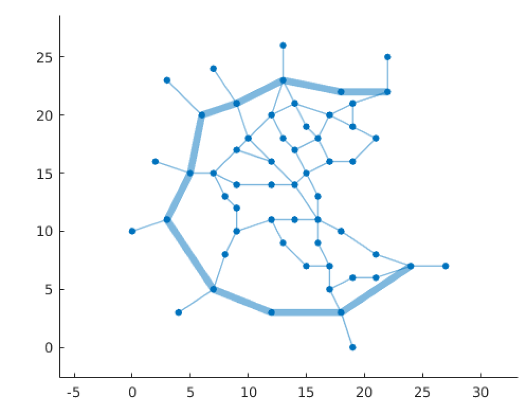
(a) Flow network $G$.

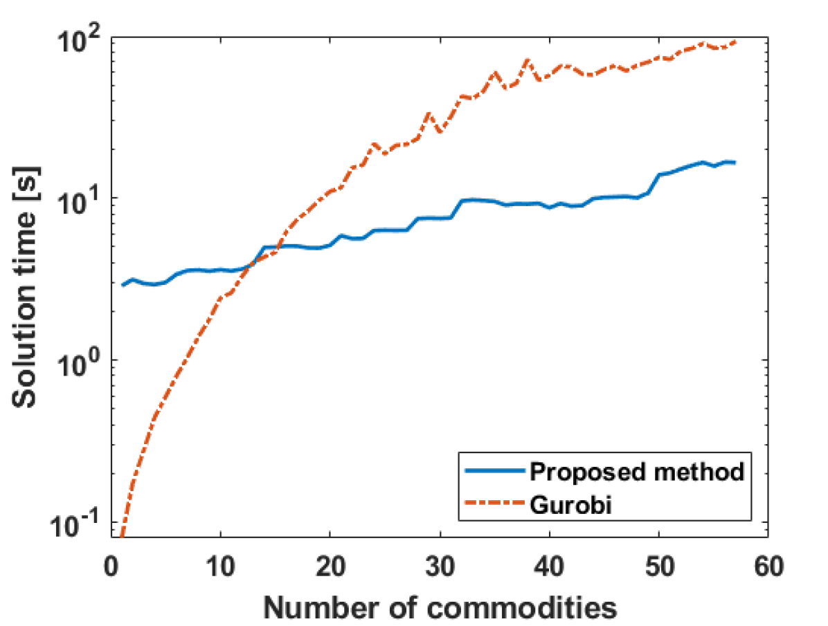
(b) Solution times for the proposed method and for Gurobi, when solving the problem in Section IV-C1.

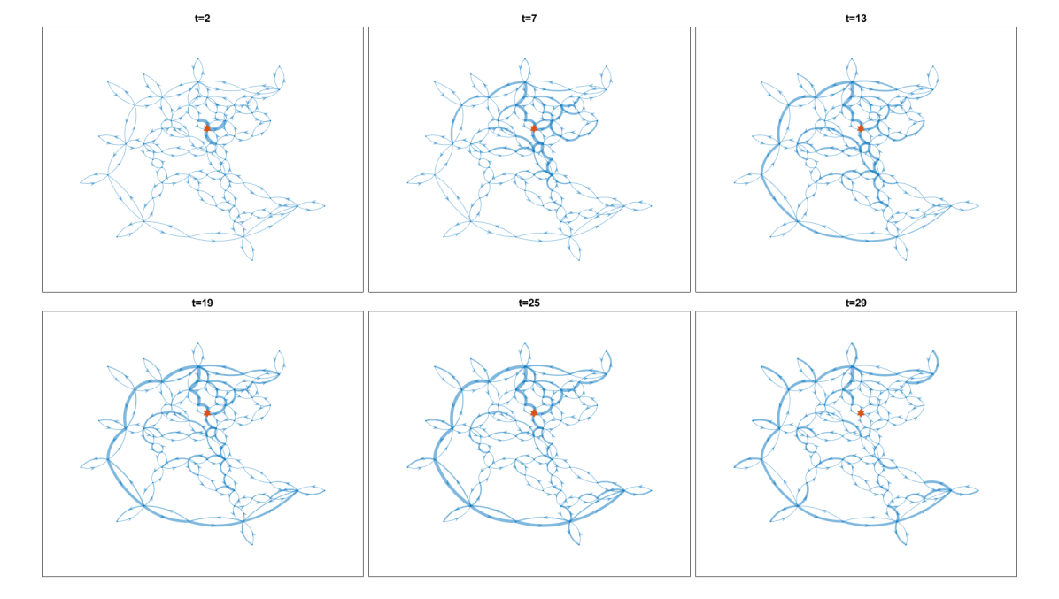
(c) An illustration of the optimal flow, using the setup in Section IV-C2, from one of the sources at a number of different time points. The width of each edge is proportional to the logarithm of $1+$ the flow on that edge at the given time point.

Figure 2: Figures for the numerical examples in Section IV-C.

V Multi-species potential mean field games

An important tool for analyzing and controlling systems of systems, which has emerged during the last decades, is mean field games [jovanovic1988anonymous, huang2006large, lasry2007mean, huang2012social, caines2018mean, djehiche2017mean]. Mean field games are models of dynamic games where each player’s action is negligible to other players at the individual level, but where the actions are significant when aggregated. A subclass of such games are potential mean field games. These can be seen as density control problems, where the density abides to a controlled Fokker-Planck equation with distributed control [lasry2007mean]. This type of control problems have been studied in, e.g., [cardaliaguet2015second, bensoussan2013mean, chen2018steering]. An important generalization of mean field games is the multi-species setting, where the population consists of several different types of agents or species [huang2006large, lasry2007mean, lachapelle2011mean, achdou2017mean, cirant2015multi, bensoussan2018mean]. In this section, we show that discretizations of potential multi-species mean field games take the form of a convex graph-structured tensor optimization problem (5). By also deriving efficient methods for computing the corresponding projections needed in Algorithm 1, we here develop an efficient numerical solution algorithm for solving such problems. In order to do so, we will first consider the nonlinear density control problem obtained in the single-species setting, and its corresponding discretization.

V-A The single-species problem

Let $X\subset{\mathbb{R}}^{n}$ be a state space, and consider a set of infinitesimal agents on $X$ which obeys the (Itô) stochastic differential equation

$$dx(t)=f(x(t))dt+B(x(t))\big{(}v(x(t),t)dt+\sqrt{\epsilon}dw\big{)},$$ (22)

subject to the initial condition $x(0)=x_{0}\sim\rho_{0}(x)$. More precisely, we assume that $f:X\to{\mathbb{R}}^{n}$ and $B:X\to{\mathbb{R}}^{n\times n}$ are continuously differentiable with bounded derivatives, in which case, under suitable conditions on the (Markovian) feedback $v$, there exists a unique solution to (22) a.s., see, e.g, [fleming1975deterministic, Thm. V.4.1], [bensoussan2013mean, pp. 7-8]. Moreover, under suitable regularity conditions [bensoussan2013mean, cardaliaguet2015second] the density $\rho(t,\cdot)$ which describe the distribution of particles at time point $t$ exists and is the solution of a controlled Fokker-Planck equation (cf. [astrom1970introduction, p. 72]). A potential mean field game can then be reformulated as the density optimal control problem [lasry2007mean]

$$\underset{\rho,v}{\text{minimize }} \int_{0}^{1}\!\!\!\int_{X}\!\frac{1}{2}\|v\|^{2}\!\rho dxdt+\!\!\int_{0}^{1}\!\!\!\mathcal{F}_{t}(\rho(t,\cdot))dt+\mathcal{G}(\rho(1,\cdot))$$ (23a)

subject to $$\,\frac{\partial\rho}{\partial t}+\nabla\cdot((f+Bv)\rho)-\frac{\epsilon}{2}\sum_{i,k=1}^{n}\frac{\partial^{2}(\sigma_{ik}\rho)}{\partial x_{i}\partial x_{k}}=0$$ (23b)

$$\,\rho(0,\cdot)=\rho_{0}.$$ (23c)

Here, $\sigma(x):=B(x)B(x)^{T}$. Moreover, $\mathcal{F}_{t}$ and $\mathcal{G}$ are functionals on $L_{2}\cap L_{\infty}$, and we assume that they are proper, convex, and lower-semicontinuous. We also assume that $\mathcal{F}_{t}$ is piece-wise continuous with respect to $t$.

To discretize problem (23), we rewrite it as a problem over path space. To this end, let ${\mathcal{P}}^{v}$ denote the distribution on path space, i.e., a probability distribution over $C([0,1],X)$ := the set of continuous functions from $[0,1]$ to $X$, induced by the controlled process (22). In particular, this means that for the marginal of ${\mathcal{P}}^{v}$ corresponding to time $t$, denoted ${\mathcal{P}}^{v}_{t}$, we have that ${\mathcal{P}}^{v}_{t}=\rho(t,\cdot)$, where $\rho$ is the solution to (23b) and (23c). Moreover, let ${\mathcal{P}}^{0}$ denote the corresponding (uncontrolled) Wiener process with initial density $\rho_{0}$. By the Girsanov theorem (see, e.g., [Follmer88, pp. 156-157], [dai1991stochastic, p. 321]), we have that

$$\frac{1}{2}\!\int_{X}\!\int_{0}^{1}\!\|v\|^{2}\rho dtdx\!=\!\frac{1}{2}{\mathbb{E}}_{{\mathcal{P}}^{v}}\left\{\int_{0}^{1}\!\|v\|^{2}dt\right\}\!=\!\epsilon{\rm KL}({\mathcal{P}}^{v}\|{\mathcal{P}}^{0})$$ (24)

where ${\rm KL}(\cdot\|\cdot)$ is the Kullback-Leibler divergence, see, e.g., [chen2016relation, gentil2017analogy, chen2018steering, BenCarDiNen19, leonard2012schrodinger, leonard2013schrodinger]. To ensure that (24) holds, it is important that the control signal and the noise enter the system through the same channel, as in (22) [chen2016optimalPartI, chen2017optimal]. Moreover, the link between stochastic control and entropy provided by (24) has recently led to several novel applications of optimal control [chen2016relation, chen2016optimalPartI, chen2017optimal, chen2020stochastic, caluya2021wasserstein].

By using (24), the problem (23) can be reformulated as

$$\underset{{\mathcal{P}}^{v}}{\text{minimize }} \quad\epsilon\,{\rm KL}({\mathcal{P}}^{v}\|{\mathcal{P}}^{0})+\int_{0}^{1}\mathcal{F}_{t}({\mathcal{P}}^{v}_{t})dt+\mathcal{G}({\mathcal{P}}^{v}_{1})$$

subject to $$\quad{\mathcal{P}}^{v}_{0}=\rho_{0}.$$

Next, we discretize this problem in both time and space. More precisely, discretizing over time into the time points $0,\Delta t,2\Delta t,\ldots,1$, where $\Delta t=1/{\mathcal{T}}$, and over space into the grid points $x_{1},\ldots,x_{N}$, the problem becomes

$$\underset{\begin{subarray}{c}{\bf M}\in{\mathbb{R}}_{+}^{N^{{\mathcal{T}}+1}}\\ \mu_{1},\ldots,\mu_{\mathcal{T}}\in{\mathbb{R}}_{+}^{N}\end{subarray}}{\text{minimize }} \;\langle{\bf C},{\bf M}\rangle+\epsilon D({\bf M})+\Delta t\!\sum_{j=1}^{{\mathcal{T}}-1}F_{j}(\mu_{j})+G(\mu_{\mathcal{T}})$$ (25a)

subject to $$\;P_{j}({\bf M})=\mu_{j},\;j=1,2,\ldots,{\mathcal{T}},$$ (25b)

$$\;P_{0}({\bf M})=\mu_{0}.$$ (25c)

Here, ${\bf M}$ is a nonnegative $({\mathcal{T}}+1)$-mode tensor that represents the flow of the agents, $\mu_{0}$ is a discrete approximation of $\rho_{0}$, and $\mu_{j}$ is the distribution of agents at time point $j$. Moreover, ${\bf C}$ is a $({\mathcal{T}}+1)$-mode tensor that represents the cost of moving agents. Since the cost of moving agents depends only on the current time step, the cost tensor takes the form

$${\bf C}_{i_{0},\ldots,i_{\mathcal{T}}}=\sum_{j=0}^{{\mathcal{T}}-1}C_{i_{j},i_{j+1}},$$ (26a)

where $$C N\times N C_{ik} x_{i} x_{k}$$ is a matrix defining the transition costs. More precisely, the elements are the (optimal) cost of moving mass from discretization point to discretization point in one time step, given by

$$C_{ik}\;=\;\begin{cases}\displaystyle\;\underset{v\in L_{2}([0,\Delta t])}{\text{minimize }}&\;\displaystyle\int_{0}^{\Delta t}\frac{1}{2}\|v\|^{2}dt\\ \;\text{subject to }&\;\displaystyle\dot{x}=f(x)+B(x)v\\ &\;\displaystyle x(0)=x_{i},\quad x(\Delta t)=x_{k}.\end{cases}$$ (26b)

The optimal control problem (26b) can typically not be solved analytically, except in the linear-quadratic case. Nevertheless, a numerical solution to the problem suffices, and the computation of the cost function $C$ can be done off-line before solving (25). In order to guarantee that the elements (26b) are all finite, we typically impose the following assumption: that the deterministic counterpart to system (22) is controllable in the (rather strong) sense that for all $x_{0},x_{1}\in X$ and for all $t>0$ there exists a control signal in $L_{2}([0,t])$ that transitions the system from the initial state $x(0)=x_{0}$ to the final state $x(t)=x_{1}$. By allowing the matrix $C$ to have elements with value $\infty$, this assumption may be relaxed. However, in this case one has to assure that (25) has a feasible solution with finite object function value, i.e., that there is an ${\bf M}\in{\mathbb{R}}_{+}^{N^{{\mathcal{T}}+1}}$ that fulfills (25b) and (25c) and is such that (25a) is finite (cf. Assumption A).

Finally, note that the problem (25)–(26) is a convex graph-structured tensor optimization problem of the form (5) on a path-graph.

Remark V.1.

Another solution method for solving problems of the form (25), for agents that follow the dynamics of a first-order integrator, has been presented in [BenCarDiNen19]. The two methods are similar, and the main difference is that the computational method developed in [BenCarDiNen19] is based on a variable elimination technique, in contrast to the belief-propagation-type technique used here; see the discussion just before Theorem III.9.

V-B The multi-species problem

A multi-species mean field game is an extension of mean field games to a set of heterogeneous agents, and the idea was already presented in the seminal work [huang2006large, lasry2007mean]. Here, we consider a multi-species potential mean field game which has $L$ different populations, each of which can be associated with different costs and constraints, and where each infinitesimal agent of species $\ell$ obeys the dynamics

$$dx_{\ell}(t)=f(x_{\ell})dt+B(x_{\ell})\big{(}v_{\ell}dt+\sqrt{\epsilon}dw_{\ell}\big{)}.$$

Next, let $\rho_{\ell}(t,\cdot)$ denote the distribution of species $\ell$ at time point $t$, and note that a multi-species potential mean field game can, analogously to the single species game, be formulated as an optimal control problem over densities. More precisely, the problem of interest here takes the form

$$\underset{\begin{subarray}{c}\rho,\rho_{\ell},v_{\ell}\end{subarray}}{\text{minimize }} \;\int_{0}^{1}\!\!\!\int_{X}\sum_{\ell=1}^{L}\frac{1}{2}\|v_{\ell}\|^{2}\rho_{\ell}\,dxdt+\!\int_{0}^{1}\!\!\mathcal{F}_{t}(\rho(t,\cdot))dt+\mathcal{G}(\rho(1,\cdot))$$

$$\quad+\sum_{\ell=1}^{L}\left(\int_{0}^{1}\mathcal{F}^{\ell}_{t}(\rho_{\ell}(t,\cdot))dt+\mathcal{G}^{\ell}(\rho_{\ell}(1,\cdot))\right)$$ (27a)

subject to $$\;\frac{\partial\rho_{\ell}}{\partial t}+\nabla\cdot((f(x)+B(x)v_{\ell})\rho_{\ell})$$

$$\quad-\frac{\epsilon}{2}\sum_{i,k=1}^{n}\frac{\partial^{2}(\sigma_{ik}\rho_{\ell})}{\partial x_{i}\partial x_{k}}=0,\quad\ell=1,\ldots L,$$ (27b)

$$\;\rho_{\ell}(0,\cdot)=\rho_{0,\ell},\quad\rho(t,x)=\sum_{\ell=1}^{L}\rho_{\ell}(t,x),$$ (27c)

where we impose the same assumptions on $\mathcal{F}^{\ell}_{t}$ and $\mathcal{G}^{\ell}$ as on $\mathcal{F}_{t}$ and $\mathcal{G}$, respectively. The functionals $\int_{0}^{1}\mathcal{F}_{t}(\cdot)dt$ and $\mathcal{G}(\cdot)$ are the cooperative part of the cost, which connects the different species. In particular, for $\mathcal{F}_{t}\equiv 0$, $\mathcal{G}\equiv 0$, (27) reduces to $L$ independent single-species problems. Moreover, the functionals $\int_{0}^{1}\mathcal{F}_{t}^{\ell}(\cdot)dt$ and $\mathcal{G}^{\ell}(\cdot)$ are the ones that give rise to the heterogeneity among the species.

V-C Numerical algorithm for solving the multi-species problem

To derive a numerical algorithm for solving (27), analogously to the single-species problem we first discretize the problem over time and space. To this end, by adapting the arguments in the previous section, we arrive at the discrete problem

$$\underset{\begin{subarray}{c}{\bf M}_{\ell},\mu_{j},\mu_{j}^{(\ell)}\\ j=1,\ldots,{\mathcal{T}}\\ \ell=1,\ldots,L\end{subarray}}{\text{minimize }} \;\sum_{\ell=1}^{L}\big{(}\langle{\bf C},{\bf M}_{\ell}\rangle+\epsilon D({\bf M}_{\ell})\big{)}+\Delta t\sum_{j=1}^{{\mathcal{T}}-1}F_{j}(\mu_{j})+G(\mu_{\mathcal{T}})$$

$$\;+\sum_{\ell=1}^{L}\left(\Delta t\sum_{j=1}^{{\mathcal{T}}-1}F_{j}^{\ell}(\mu_{j}^{(\ell)})+G^{\ell}(\mu_{\mathcal{T}}^{(\ell)})\right)$$ (28a)

subject to $$\;P_{j}({\bf M}_{\ell})=\mu_{j}^{(\ell)},\;j=1,\ldots,{\mathcal{T}},\,\ell=1,\ldots,L,$$ (28b)

$$\;P_{0}({\bf M}_{\ell})=\mu_{0,\ell},\;\ell=1,\ldots,L,$$ (28c)

$$\;\sum_{\ell=1}^{L}\mu_{j}^{(\ell)}=\mu_{j},\;j=0,\ldots,{\mathcal{T}}$$ (28d)

where ${\bf C}$ still has the form (26), and where $\mu_{0,\ell}$ are discrete approximations of $\rho_{0,\ell}$. In particular, note that the second line in the cost (28a) is the discretization of the second line in (27a). Moreover, also note that (28) consists of $L$ coupled multi-marginal optimal transport problems, coupled via the constraint (28d) and the cost imposed on $\mu_{j}$, for $j=1,\ldots,{\mathcal{T}}$, in (28a).

Next, we reformulate (28) into one single entropy-regularized multi-marginal transport problem (cf. [haasler2021scalable]). To this end, let ${\bf M}\in{\mathbb{R}}^{L\times N^{{\mathcal{T}}+1}}$ be the $({\mathcal{T}}+2)$-mode tensor such that ${\bf M}_{\ell i_{0}\dots i_{\mathcal{T}}}=({\bf M}_{\ell})_{i_{0}\dots i_{\mathcal{T}}}$, i.e., ${\bf M}_{\ell i_{0}\dots i_{\mathcal{T}}}$ is the amount of mass of species $\ell$ that moves along the path $x_{i_{0}},\dots,x_{i_{\mathcal{T}}}$. For this tensor ${\bf M}$, we will use the index $-1$ to denote the “species index”. This means that $(P_{-1}({\bf M}))_{\ell}=\sum_{i_{0},\ldots,i_{\mathcal{T}}}({\bf M}_{\ell})_{i_{0}\dots i_{\mathcal{T}}}$, for $\ell=1,\ldots,L$, and hence the elements of the additional marginal $\mu_{-1}\in{\mathbb{R}}_{+}^{L}$ are the total mass of the densities of the different species. Moreover, this means that $P_{j}({\bf M})$ is the total distribution $\mu_{j}$ at time $j\Delta t$, as defined by (28d), while the bimarginal projection $P_{-1,j}({\bf M})$ gives the $L\times N$ matrix $[\mu_{j}^{(1)},\ldots,\mu_{j}^{(L)}]^{T}$. By introducing the matrix

$$\mathfrak{R}^{(-1,0)}=[\mu_{0,1},\ldots,\mu_{0,L}]^{T}\in{\mathbb{R}}_{+}^{L\times N},$$

the constraint (28c) can be imposed by requiring that $P_{-1,0}({\bf M})=\mathfrak{R}^{(-1,0)}$. Next, by defining the functions $\mathscr{F}_{j}^{L}:{\mathbb{R}}^{L\times N}\to{\mathbb{R}}$ as

$$\mathscr{F}_{j}^{L}(R^{(-1,j)})=\sum_{\ell=1}^{L}\Delta tF_{j}^{\ell}(\mu_{j}^{(\ell)})\quad j=1,\ldots,{\mathcal{T}},$$

and similarly for $\mathscr{G}^{L}$, the last term in the cost (28a) can be written as functionals applied to the bimarginal projections. Finally, by noting that $\sum_{\ell=1}^{L}D({\bf M}_{\ell})=D({\bf M})$, we can write the problem as

$$\underset{\begin{subarray}{c}{\bf M},\mu_{j},R^{(-1,j)}\\ j=1,\ldots,{\mathcal{T}}\end{subarray}}{\text{minimize }} \;\langle\tilde{{\bf C}},{\bf M}\rangle+\epsilon D({\bf M})+\Delta t\sum_{j=1}^{{\mathcal{T}}-1}F_{j}(\mu_{j})+G(\mu_{\mathcal{T}})$$

$$\;+\sum_{j=1}^{{\mathcal{T}}-1}\mathscr{F}_{j}^{L}(R^{(-1,j)})+\mathscr{G}^{L}(R^{(-1,{\mathcal{T}})})$$ (29a)

subject to $$\;P_{j}({\bf M})=\mu_{j},\quad j=1,\ldots,{\mathcal{T}},$$ (29b)

$$\;P_{-1,j}({\bf M})=R^{(-1,j)},\quad j=1,\ldots,{\mathcal{T}},$$ (29c)

$$\;P_{-1,0}({\bf M})=\mathfrak{R}^{(-1,0)}$$ (29d)

where

$$\tilde{{\bf C}}_{\ell i_{0}\ldots i_{\mathcal{T}}}=\sum_{j=0}^{{\mathcal{T}}-1}C_{i_{j},i_{j+1}}.$$ (29e)

The problem (29) is readily seen to be a graph-structured entropy-regularized multi-marginal optimal transport problem of the form (5), and can hence be solved using Algorithm 1. In particular, the iterates of the transport plan produced by Algorithm 1 are of the form ${\bf M}^{k}={\bf K}\odot{\bf U}^{k}$, where ${\bf K}=\exp(-\tilde{{\bf C}}/\epsilon)$ and where

$${\bf U}_{\ell i_{0}\dots i_{\mathcal{T}}}=U_{-1,0}^{(\ell,i_{0})}\prod_{j=1}^{\mathcal{T}}U_{-1,j}^{(\ell,i_{j})}\prod_{j=1}^{\mathcal{T}}u_{j}^{(i_{j})}.$$ (30)

The underlying graph-structure is illustrated in Figure 3, and by adapting the arguments in [haasler2021scalable], marginal and bimarginal projections needed in the inclusion problems (15) can be computed efficiently as follows.

Theorem V.2.

Let ${\bf K}=\exp(-\tilde{{\bf C}}/\epsilon)$, with $\tilde{{\bf C}}$ defined as in (29e) and $\epsilon>0$, and let ${\bf U}$ be as in (30). Define $K=\exp(-C/\epsilon)$, and let

$$\hat{\Psi}_{j}=\begin{cases}U_{-1,0}K,&j=1,\\ \left(\hat{\Psi}_{j-1}\odot U_{-1,j-1}\right)\mathrm{diag}(u_{j-1})K,&j=2,\dots,{\mathcal{T}},\end{cases}$$

and

$$\Psi_{j}=\begin{cases}U_{-1,{\mathcal{T}}}\,\mathrm{diag}(u_{\mathcal{T}})K^{T},&j={\mathcal{T}}-1,\\ \left(\Psi_{j+1}\odot U_{-1,j+1}\right)\mathrm{diag}(u_{j+1})K^{T},&j=0,\dots,{\mathcal{T}}-2.\end{cases}$$

Then we have the following expressions for projections of the tensor ${\bf K}\odot{\bf U}$

$$P_{-1,0}({\bf K}\odot{\bf U})=U_{-1,0}\odot\Psi_{0},$$

$$P_{-1,j}({\bf K}\odot{\bf U})=\hat{\Psi}_{j}\odot\Psi_{j}\odot U_{-1,j}\mathrm{diag}(u_{j}),$$

$$P_{-1,{\mathcal{T}}}({\bf K}\odot{\bf U})=U_{-1,{\mathcal{T}}}\mathrm{diag}(u_{\mathcal{T}})\odot\hat{\Psi}_{{\mathcal{T}}},$$

$$P_{\mathcal{T}}({\bf K}\odot{\bf U})=u_{\mathcal{T}}\odot\left(\hat{\Psi}_{{\mathcal{T}}}\odot U_{-1,{\mathcal{T}}}\right)^{T}{\bf 1},$$

$$P_{j}({\bf K}\odot{\bf U})=u_{j}\odot\left(\hat{\Psi}_{j}\odot\Psi_{j}\odot U_{-1,j}\right)^{T}{\bf 1},$$

for $j=1,\dots,{\mathcal{T}}-1$.

Proof.

See Appendix -A. ∎

Finally, using Theorem V.2 and specializing Algorithm 1 to solving the particular problem (29), an algorithm for solving discretized multi-species potential mean field games is given in Algorithm 3.

Remark V.3.

The algorithms in [ringh2021efficient] are special instances of Algorithm 3. In particular, if $\mathscr{F}_{j}^{L}(\cdot)=\langle C_{j},\cdot\rangle$ for some $C_{j}\in{\mathbb{R}}^{L\times N}$, then $(\mathscr{F}_{j}^{L})^{*}(\cdot)=I_{\{C_{j}\}}(\cdot)$. Hence, $U_{-1,j}$ must equal $K_{j}:=\exp(-C_{j}/\epsilon)$. Similarly, if $\mathscr{G}^{L}(\cdot)=\langle C_{\mathcal{T}},\cdot\rangle$, we get that $U_{-j,{\mathcal{T}}}$ must be equal to $K_{\mathcal{T}}$, from which we recover [ringh2021efficient, Alg. 1]. On the other hand, if $\mathscr{G}^{L}(\cdot)=I_{\{\mathfrak{R}^{(-1,{\mathcal{T}})}\}}(\cdot)$ for some given $\mathfrak{R}^{(-1,{\mathcal{T}})}$, then the marginal $\mu_{\mathcal{T}}$ is also known and any cost associated with it is a constant and can hence be removed. Moreover, $(\mathscr{G}^{L})^{*}(\cdot)=\langle\mathfrak{R}^{(-1,{\mathcal{T}})},\cdot\rangle$, from which we recover [ringh2021efficient, Alg. 2].

0:  Initial guess $u_{1},\dots,u_{{\mathcal{T}}}$, $U_{-1,0},\ldots,U_{-1,{\mathcal{T}}}$

1:  $\Psi_{{\mathcal{T}}-1}\leftarrow U_{-1,{\mathcal{T}}}\,\mathrm{diag}(u_{\mathcal{T}})K^{T}$

2:  for  $j={\mathcal{T}}-2,\dots,0$ do

3:     $\Psi_{j}\leftarrow(\Psi_{j+1}\odot U_{-1,j+1})\mathrm{diag}(u_{j+1})K^{T}$

4:  end for

5:  while Not converged do

6:     $U_{-1,0}\leftarrow\mathfrak{R}^{(-1,0)}\oslash\Psi_{0}$

7:     $\hat{\Psi}_{1}\leftarrow U_{-1,0}K$

8:     for  $j=1,\dots,{\mathcal{T}}-1$ do

9:        $W_{-1,j}\leftarrow(\hat{\Psi}_{j}\odot\Psi_{j})\mathrm{diag}(u_{j})$

10:        Update $U_{-1,j}$ by $0=-U_{-1,j}\odot W_{-1,j}+\partial(\mathscr{F}_{j}^{L})^{*}(-\epsilon\log(U_{-1,j}))$.

11:        $w_{j}\leftarrow(\hat{\Psi}_{j}\odot\Psi_{j}\odot U_{-1,j})^{T}{\bf 1}$

12:        Update $u_{j}$ by $0=-u_{j}\odot w_{j}+\partial(\Delta tF_{j})^{*}(-\epsilon\log(u_{j}))$.

13:        $\hat{\Psi}_{j+1}\leftarrow(\hat{\Psi}_{j}\odot U_{-1,j})\mathrm{diag}(u_{j})K$

14:     end for

15:     $W_{-1,{\mathcal{T}}}\leftarrow\hat{\Psi}_{{\mathcal{T}}}\mathrm{diag}(u_{\mathcal{T}})$

16:     Update $U_{-1,{\mathcal{T}}}$ by $0=-U_{-1,{\mathcal{T}}}\odot W_{-1,{\mathcal{T}}}+\partial(\mathscr{G}^{L})^{*}(-\epsilon\log(U_{-1,{\mathcal{T}}}))$.

17:     $w_{{\mathcal{T}}}\leftarrow(\hat{\Psi}_{{\mathcal{T}}}\odot U_{-1,{\mathcal{T}}})^{T}{\bf 1}$

18:     Update $u_{\mathcal{T}}$ by $0=-u_{{\mathcal{T}}}\odot w_{{\mathcal{T}}}+\partial G^{*}(-\epsilon\log(u_{\mathcal{T}}))$.

19:     $\Psi_{{\mathcal{T}}-1}\leftarrow U_{-1,{\mathcal{T}}}\,\mathrm{diag}(u_{\mathcal{T}})K^{T}$

20:     for $j={\mathcal{T}}-1,\dots,1$ do

21:        $\Psi_{j-1}\leftarrow(\Psi_{j}\odot U_{-1,j})\mathrm{diag}(u_{j})K^{T}$

22:     end for

23:  end while

23:  $u_{1},\dots,u_{{\mathcal{T}}}$, $U_{-1,0},\ldots,U_{-1,{\mathcal{T}}}$

Algorithm 3 Method for solving the multi-species potential mean field game (29).

Figure 3: Illustration of the graph ${\mathcal{G}}$ for the multi-species density optimal control problem. Grey circles correspond to known densities, and white circles correspond to densities which are to be optimized over.

V-D Numerical example

In this section we demonstrate Algorithm 3 on a two-dimensional numerical example with $L=4$ different species. To this end, we consider the state space $[0,3]\times[0,3]$ and uniformly discretize it into $100\times 100$ grid points; the latter are denoted $x_{i,k}$ for $i,k=1,\ldots,100$. No points are placed on the boundary of the state space, which means that the cell size is $\Delta x=0.03^{2}$. Moreover, time is discretized into ${\mathcal{T}}+1=40$ time steps, i.e., with a discretization size $\Delta t=1/39$ and with time index $j=0,\ldots,39$. The dynamics of the agents is taken to be $f(x)\equiv 0$ and $B(x)=I$. This means that the cost matrix, with elements (26b), is time-independent and given by $C=[\|x_{i_{1},k_{1}}-x_{i_{2},k_{2}}\|^{2}]_{i_{1},i_{2},k_{1},k_{2}=1}^{100}$. This corresponds to the squared Wasserstein-2 distance on the discrete grid.

For $\epsilon=10^{-2}$, we consider the discrete problem

$$\underset{\begin{subarray}{c}{\bf M}_{\ell}\in{\mathbb{R}}_{+}^{100^{40}},\\ \mu_{j}^{(\ell)}\in{\mathbb{R}}_{+}^{100}\\ j=1,\ldots,39,\;\ell=1,2,3,4\end{subarray}}{\text{minimize }} \quad\sum_{\ell=1}^{4}\Big{(}\langle{\bf C},{\bf M}_{\ell}\rangle+\epsilon D({\bf M}_{\ell})\Big{)}$$

$$\quad+\sum_{j=1}^{39}\langle c_{3},\mu_{j}^{(3)}\rangle+0.1\sum_{j=1}^{39}\|\mu_{j}^{(4)}-\tilde{\mu}^{(4)}\|_{2}^{2}$$

$$\quad+3\|\mu_{19}-\tilde{\mu}_{1}\|^{2}_{2}+3\|\mu_{39}-\tilde{\mu}_{2}\|^{2}_{2}$$ (31a)

subject to $$\quad P_{j}({\bf M}_{\ell})=\mu_{j}^{(\ell)},\quad j=0,\ldots,39,$$

$$\quad\phantom{P_{j}({\bf M}_{\ell})=\mu_{j}^{(\ell)},}\quad\ell=1,2,3,4,$$ (31b)

$$\quad\sum_{\ell=1}^{4}\mu_{j}^{(\ell)}=\mu_{j},\quad j=0,\ldots,39,$$ (31c)

$$\quad\mu_{j}\leq\kappa_{j},\quad j=1,\ldots,39,$$ (31d)

$$\quad\mu_{j}^{(1)}\leq\kappa^{(1)},\quad j=1,\ldots,39.$$ (31e)

Here, $\tilde{\mu}_{1}$ and $\tilde{\mu}_{2}$ are the two distributions given in Figure 4(a). Moreover, the linear cost $c_{3}$, associated with species $3$, and the target distribution $\tilde{\mu}^{(4)}$, associated with species $4$, are both given in Figure 4(b). Finally, for the capacity constraint (31d), $\kappa_{j}$ is illustrated in Figure 4(c), while for the capacity constraint (31e), $\kappa^{(1)}$ is zero in the lower half of the domain and infinite for the upper half.

The multi-marginal optimal transport reformulation of (31) was solved using Algorithm 3. The latter is adapted as in Section III-D to handle both the costs on the total marginals in (31a) and the inequality constraints in (31d); details on the Fenchel conjugates of the functions involved can be found in Table I. Results are shown in Figure 5, where the initial distributions $\mu_{0}^{(\ell)}$ for the different agents can be seen in the left-most column (showing time point $j=0$).

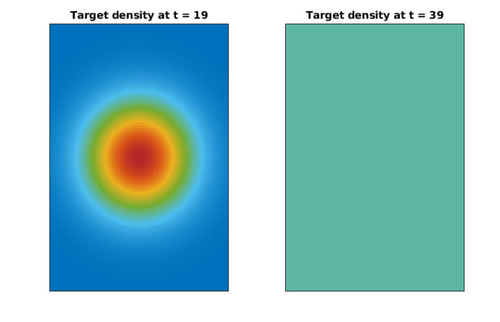
(a) Target densities $\tilde{\mu}_{1}$ (left) and $\tilde{\mu}_{2}$ (right) for the total density at time points $j=19$ and $j=39$, respectively.

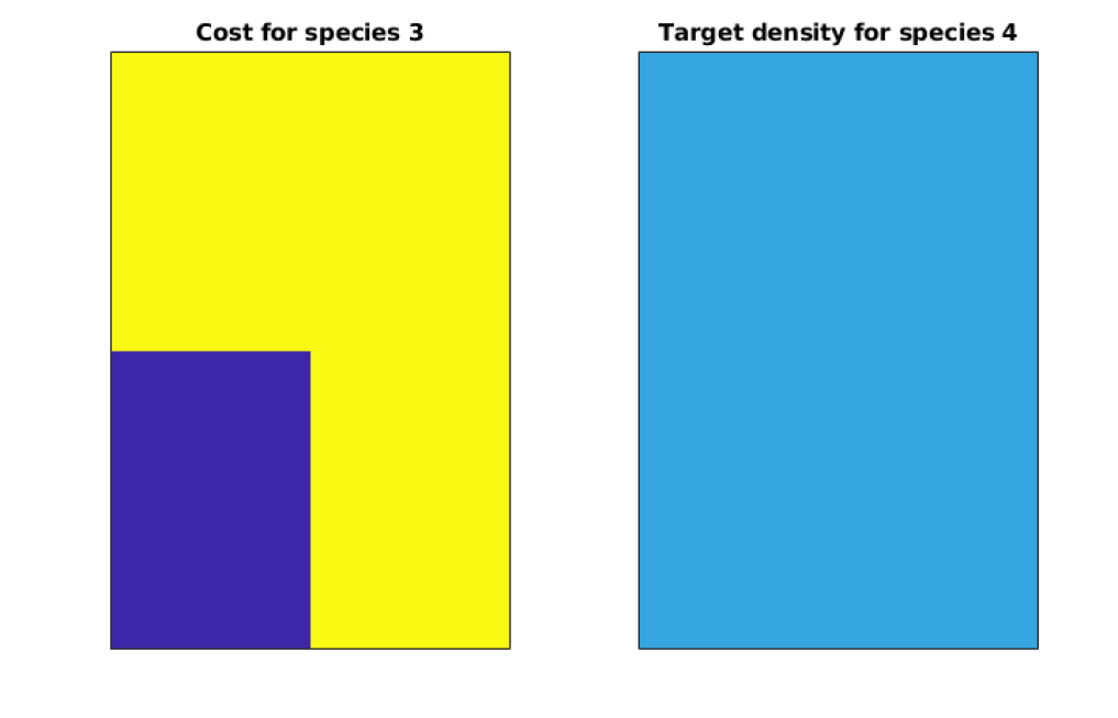
(b) The left plot shows the linear cost $c_{3}$ for species $3$, where blue means cost 0 and yellow means a cost of $390\Delta x\Delta t$. The right plots shows the target distributions $\tilde{\mu}^{(4)}$ for species $4$.

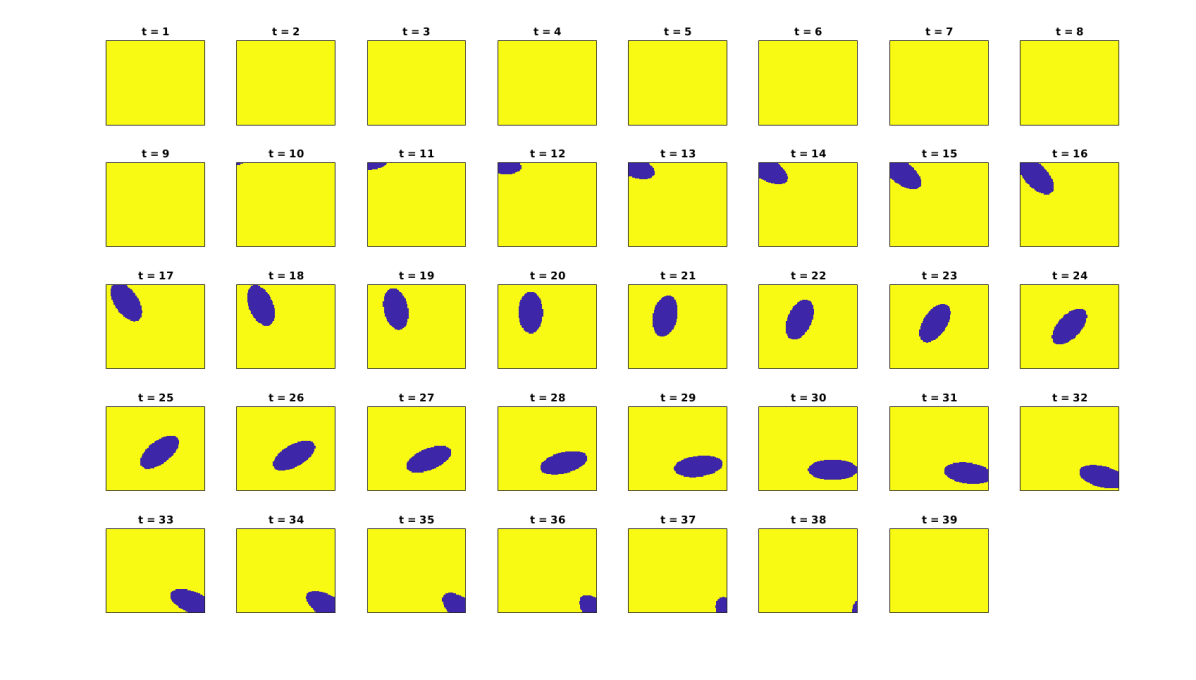
(c) Illustration of the capacity constraints $\kappa_{j}$ at the different time points $j$: blue means zero capacity (obstacle) while yellow means infinite capacity.

Figure 4: Figures describing the setup in the numerical example in Section V-D.

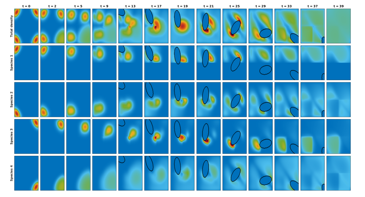
Figure 5: Time evolution of total density and densities of the individual species, for the numerical example in Section V-D.

VI Conclusions

In this paper we have seen that graph structured tensor optimization problems naturally appear in several areas in systems and control. We have developed numerical algorithms for these problems based on dual coordinate ascent that utilize the fact that the dual problems decouple according to the graph structure. We also showed that under mild conditions these algorithms are globally convergent, and in certain cases the convergence is R-linear. We believe that these methods are useful for addressing many other types of problems, e.g., in flow problems where the nodes or edges also have dynamics (cf. [como2017resilient]). Moreover, we also believe that these methods can be extended to handle, e.g., multi-species potential mean field games where each species also has different dynamics.

-A Deferred proofs

Proof of Lemma III.3.

By Assumption A, there is a feasible point to (5) with finite objective function value, and since problems (5) and (4) are equivalent, this means that the objective function in (4) is proper. To show that the minimum for the latter is attained, note that $g^{(t)}$, $t\in{\mathcal{V}}$, and $f^{(t_{1},t_{2})}$, $(t_{1},t_{2})\in{\mathcal{E}}$, are all proper, convex, and lower-semicontinuous, and hence they all have a continuous affine minorant [bauschke2017convex, Thm. 9.20]. However, and since the entropy term $\epsilon D({\bf M})$ is radially unbounded and grows faster towards $\infty$ than linearly, we have that the objective function in (4) is radially unbounded. Since the entire objective function is also proper, convex, and lower-semicontinuous, the minimum is attained [rockafellar1970convex, Thm. 27.2], and it is unique since $D({\bf M})$ (and hence the entire objective function in (4)) is strictly convex. ∎

Lemma .1.

Let $f:{\mathbb{R}}^{n}\to{\bar{{\mathbb{R}}}}$ be proper, convex, and lower-semicontinuous, then $\text{ri}(\text{dom}(f^{*}))\neq\emptyset$.

Proof.

Since $f$ is proper, convex, and lower-semicontinuous, so is $f^{*}$ [bauschke2017convex, Cor. 13.38]. $\text{dom}(f^{*})$ is therefore nonempty, and by [bauschke2017convex, Prop. 8.2] it is convex. Using [bauschke2017convex, Fact 6.14(i)], the result follows. ∎

Lemma .2.

There is no duality gap between (5) and (6).

Proof.

To prove it, we derive a Lagrangian dual to an equivalent problem to (6), and show that for the latter strong duality holds with (5). To this end, note that a problem with the same set of globally optimal solutions as (6) is the constrained optimization problem

$$\underset{{\bf U},\lambda,\Lambda}{\text{sup }} \;-\epsilon\langle{\bf K},{\bf U}\rangle-\sum_{t\in{\mathcal{V}}}(g^{(t)})^{*}(-\lambda_{t})-\!\!\!\!\sum_{(t_{1},t_{2})\in{\mathcal{E}}}(f^{(t_{1},t_{2})})^{*}(-\Lambda_{t_{1},t_{2}})$$

s.t. $$\quad\log({\bf U}_{i_{1}\ldots i_{{\mathcal{T}}}})=\frac{1}{\epsilon}\left(\sum_{t\in{\mathcal{V}}}\lambda_{t}^{(i_{t})}+\!\sum_{(t_{1},t_{2})\in{\mathcal{E}}}\Lambda_{t_{1},t_{2}}^{(i_{t_{1}},i_{t_{2}})}\right).$$

However, the latter is nonconvex due to the nonaffine equality constraint. Nevertheless, since ${\bf K}\geq 0$ the cost function is nonincreasing in ${\bf U}$, and since the logarithm is a monotone increasing function, the above problem has the same globally optimal solution as the relaxed, convex problem with the equality changed for an inequality $\geq$. Moreover, for this convex problem, by using Lemma .1 it is easily seen that Slater’s condition is fulfilled, and hence strong duality holds. Next, relaxing the convex inequality constraints with multipliers $\mathbf{Q}_{i_{1}\ldots i_{{\mathcal{T}}}}\geq 0$ we get the Lagrangian

$$-\epsilon\langle{\bf K},{\bf U}\rangle-\sum_{t\in{\mathcal{V}}}(g^{(t)})^{*}(-\lambda_{t})-\sum_{(t_{1},t_{2})\in{\mathcal{E}}}(f^{(t_{1},t_{2})})^{*}(-\Lambda_{t_{1},t_{2}})$$

$$+\!\!\sum_{i_{1}\ldots i_{{\mathcal{T}}}}\!\mathbf{Q}_{i_{1}\ldots i_{{\mathcal{T}}}}\!\!\left(\!\log({\bf U}_{i_{1}\ldots i_{{\mathcal{T}}}})-\frac{1}{\epsilon}\!\left(\sum_{t\in{\mathcal{V}}}\lambda_{t}^{(i_{t})}+\!\!\!\!\sum_{(t_{1},t_{2})\in{\mathcal{E}}}\!\!\!\!\Lambda_{t_{1},t_{2}}^{(i_{t_{1}},i_{t_{2}})}\!\right)\!\!\right)$$

which separates over $\lambda_{t}$, $\Lambda_{t_{1},t_{2}}$, and ${\bf U}$. Moreover, we have that $\sum_{i_{1}\ldots i_{{\mathcal{T}}}}\mathbf{Q}_{i_{1}\ldots i_{{\mathcal{T}}}}\frac{1}{\epsilon}\lambda_{t}^{(i_{t})}=\langle 1/\epsilon P_{t}(\mathbf{Q}),\lambda_{t}\rangle$, and therefore when taking the supremum over $\lambda_{t}$ we get

$$\sup_{\lambda_{t}\in{\mathbb{R}}^{N}}-(g^{(t)})^{*}(-\lambda_{t})-\langle 1/\epsilon P_{t}(\mathbf{Q}),\lambda_{t}\rangle =(g^{(t)})^{**}(1/\epsilon P_{t}(\mathbf{Q}))$$

$$=g^{(t)}(1/\epsilon P_{t}(\mathbf{Q})),$$

where the last equality follows from [bauschke2017convex, Thm. 13.37]; an analogous result holds for $(f^{(t_{1},t_{2})})^{*}$ and $\Lambda_{t_{1},t_{2}}$. The remaining part of the Lagrangian is $\sup_{{\bf U}\in{\mathbb{R}}^{N^{\mathcal{T}}}}-\epsilon\langle{\bf K},{\bf U}\rangle+\langle\mathbf{Q},\log({\bf U})\rangle$, and to find this supremum we first note that if ${\bf K}_{i_{1}\ldots i_{{\mathcal{T}}}}=0$, then we must have $\mathbf{Q}_{i_{1}\ldots i_{{\mathcal{T}}}}=0$ or else the cost function is unbounded. For all other elements, we take the derivative with respect to ${\bf U}_{i_{1}\ldots i_{{\mathcal{T}}}}$ and set it equal to zero, from which it follows that ${\bf U}_{i_{1}\ldots i_{{\mathcal{T}}}}=\mathbf{Q}_{i_{1}\ldots i_{{\mathcal{T}}}}/(\epsilon{\bf K}_{i_{1}\ldots i_{{\mathcal{T}}}})>0$, which is hence the supremum. Plugging this back into the cost, we get

$$-\epsilon\langle{\bf K},{\bf U}\rangle+\langle\mathbf{Q},\log({\bf U})\rangle$$

$$\quad=\sum_{i_{1}\ldots i_{{\mathcal{T}}}}-\mathbf{Q}_{i_{1}\ldots i_{{\mathcal{T}}}}+\langle\mathbf{Q},\log(\mathbf{Q})\rangle-\langle\mathbf{Q},\log(\epsilon{\bf K})\rangle$$

$$\quad=\sum_{i_{1}\ldots i_{{\mathcal{T}}}}-\mathbf{Q}_{i_{1}\ldots i_{{\mathcal{T}}}}+\langle\mathbf{Q},\log(\mathbf{Q})-\log(\epsilon)\rangle+(1/\epsilon)\langle\mathbf{Q},{\bf C}\rangle,$$

together with the constraints that $\mathbf{Q}_{i_{1}\ldots i_{{\mathcal{T}}}}=0$ if ${\bf K}_{i_{1}\ldots i_{{\mathcal{T}}}}=0$. But for any element such that ${\bf K}_{i_{1}\ldots i_{{\mathcal{T}}}}=0$ we have that ${\bf C}_{i_{1}\ldots i_{{\mathcal{T}}}}=\infty$, and the constraints can thus be removed since they are implicitly enforced by the cost function. Therefore, with the change of variable $\mathbf{Q}=\epsilon{\bf M}$ we recover, up to a constant, the primal problem (4). Since (4) has the same optimal value as (5), the result follows. ∎

Proof of Theorem V.2.

Note that ${\bf K}_{\ell i_{0}\ldots i_{\mathcal{T}}}=\prod_{t=0}^{{\mathcal{T}}-1}K_{i_{t},i_{t+1}}$. Together with (30), this means that

$$(P_{-1,j}({\bf K}\odot{\bf U}))_{\ell,i_{j}}=\sum_{\begin{subarray}{c}i_{0},\ldots i_{j-1}\\ i_{j+1},\ldots i_{{\mathcal{T}}}\end{subarray}}\Bigg{(}\left(\prod_{t=0}^{{\mathcal{T}}-1}K_{i_{t},i_{t+1}}U_{-1,0}^{(\ell,i_{0})}\right)$$

$$\;\left(\prod_{t=1}^{\mathcal{T}}U_{-1,t}^{(\ell,i_{t})}\right)\left(\prod_{t=1}^{\mathcal{T}}u_{t}^{(i_{t})}\right)\Bigg{)}=U_{-1,j}^{(\ell,i_{j})}u_{j}^{(i_{j})}\hat{\Psi}_{j}^{(\ell,j)}\Psi_{j}^{(\ell,j)},$$

where

$$\hat{\Psi}_{j}^{(\ell,i_{j})} =\sum_{i_{0},\ldots i_{j-1}}U_{-1,0}^{(\ell,i_{0})}K_{i_{0},i_{1}}\prod_{t=1}^{j-1}U_{-1,t}^{(\ell,i_{t})}u_{t}^{(i_{t})}K_{i_{t},i_{t+1}},$$

$$\Psi_{j}^{(\ell,i_{j})} =\!\sum_{i_{j+1},\ldots i_{{\mathcal{T}}}}\!U_{-1,{\mathcal{T}}}^{(\ell,i_{{\mathcal{T}}})}u_{\mathcal{T}}^{(i_{\mathcal{T}})}K_{i_{{\mathcal{T}}-1},i_{{\mathcal{T}}}}\!\prod_{t=j+1}^{{\mathcal{T}}-1}\!U_{-1,t}^{(\ell,i_{t})}u_{t}^{(i_{t})}K_{i_{t-1},i_{t}}.$$

A direct calculation gives that $\hat{\Psi}_{j}$ and $\Psi_{j}$ above fulfill the recursive definitions in the theorem, which proves the form of the bimarginal projection for $j=1,\ldots,{\mathcal{T}}-1$. Next, the form of the bimarginal projections for $j=0$ and ${\mathcal{T}}$ can be readily verified analogously. Finally, note that

$$(P_{j}({\bf K}\odot{\bf U}))_{i_{j}}=\sum_{\ell=1}^{L}(P_{-1,j}({\bf K}\odot{\bf M}))_{\ell,i_{j}},$$

which gives the result for the projections and proves the theorem. ∎