Copy, Right? A Testing Framework for Copyright Protection of Deep Learning Models

Abstract

Deep learning models, especially those large-scale and high-performance ones, can be very costly to train, demanding a considerable amount of data and computational resources. As a result, deep learning models have become one of the most valuable assets in modern artificial intelligence. Unauthorized duplication or reproduction of deep learning models can lead to copyright infringement and cause huge economic losses to model owners, calling for effective copyright protection techniques. Existing protection techniques are mostly based on watermarking, which embeds an owner-specified watermark into the model. While being able to provide exact ownership verification, these techniques are 1) invasive, i.e., they need to tamper with the training process, which may affect the model utility or introduce new security risks into the model; 2) prone to adaptive attacks that attempt to remove/replace the watermark or adversarially block the retrieval of the watermark; and 3) not robust to the emerging model extraction attacks. Latest fingerprinting work on deep learning models, though being non-invasive, also falls short when facing the diverse and ever-growing attack scenarios.

In this paper, we propose a novel testing framework for deep learning copyright protection: DeepJudge. DeepJudge quantitatively tests the similarities between two deep learning models: a victim model and a suspect model. It leverages a diverse set of testing metrics and efficient test case generation algorithms to produce a chain of supporting evidence to help determine whether a suspect model is a copy of the victim model. Advantages of DeepJudge include: 1) non-invasive, as it works directly on the model and does not tamper with the training process; 2) efficient, as it only needs a small set of seed test cases and a quick scan of the two models; 3) flexible, i.e., it can easily incorporate new testing metrics or test case generation methods to obtain more confident and robust judgement; and 4) fairly robust to model extraction attacks and adaptive attacks. We verify the effectiveness of DeepJudge under three typical copyright infringement scenarios, including model finetuning, pruning and extraction, via extensive experiments on both image classification and speech recognition datasets with a variety of model architectures.

I Introduction

Deep learning models, e.g., deep neural networks (DNNs), have become the standard models for solving many complex real-world problems, such as image recognition [18], speech recognition [15], natural language processing [7], and autonomous driving [5]. However, training large-scale DNN models is by no means trivial, which requires not only large-scale datasets but also significant computational resources. The training cost can grow rapidly with task complexity and model capacity. For instance, it can cost $1.6 million to train a BERT model on Wikipedia and Book corpora (15 GB) [37]. It is thus of utmost importance to protect DNNs from unauthorized duplication or reproduction.

One concerning fact is that well-trained DNNs are often exposed to the public via remote services (APIs), cloud platforms (e.g., Amazon AWS, Google Cloud and Microsoft Azure), or open-source toolkits like OpenVINO. It gives rise to adversaries (e.g., a model “thief”) who attempt to steal the model in stealthy ways, causing copyright infringement and economic losses to the model owners. Recent studies have shown that stealing a DNN can be done very efficiently without leaving obvious traces [38, 33]. Arguably, unauthorized finetuning or pruning is the most straightforward way of model stealing, if the model parameters are publicly accessible (for research purposes only) or the adversary is an insider. Even when only the API is exposed, the adversary can still exploit advanced model extraction techniques [38, 33, 32, 21, 45] to steal most functionalities of the hidden model. These attacks pose serious threats to the copyright of deep learning models, calling for effective protection methods.

A number of defense techniques have been proposed to protect the copyright of DNNs, where DNN watermarking [40, 47, 1, 9] is one major type of technique. DNN watermarking embeds a secret watermark (e.g., logo or signature) into the model by exploiting the over-parameterization property of DNNs [1]. The ownership can then be verified when the same or similar watermark is extracted from a suspect model. The use of watermarks has an obvious advantage, i.e., the owner identity can be embedded and verified exactly, given that the watermark can be fully extracted. However, these methods still suffer from certain weaknesses. Arguably, the most concerning one is that they are invasive, i.e., they need to tamper with the training procedure to embed the watermark, which may compromise model utility or introduce new security threats into the model [25, 41, 10, 17].

More recently, DNN fingerprinting [2, 27] has been proposed as a non-invasive alternative to watermarking. Lying at the design core of fingerprinting is uniqueness — the unique feature of a DNN model. Specifically, fingerprinting extracts a unique identifier (or fingerprint) from the owner model to differentiate it from other models. The ownership can be claimed if the identifier of the owner model matches with that of a suspect model. However, in the context of deep learning, a single fingerprinting feature/metric can hardly be sufficient or flexible enough to handle all the randomness in DNNs or against different types of model stealing and adaptive attacks (as we will show in our experiments). In other words, there exist many scenarios where a DNN model can easily lose its unique feature or property (i.e., fingerprint).

In this work, we propose a testing approach for DNN copyright protection. Instead of solely relying on one metric, we propose to actively test the “similarities” between a victim model and a suspect model from multiple angles. The core idea is to 1) carefully construct a set of test cases to comprehensively characterize the victim model, and 2) measure how similarly the two models behave on the test cases. Intuitively, if a suspect model is a stolen copy of the victim model, it will behave just like the victim model in certain ways. An extreme case is that the suspect is the exact duplicate of the victim model, and in this case, the two models will behave identically on these test cases. This testing view creates a dilemma for the adversary as better stealing will inevitably lead to higher similarities to the victim model. We further identify two major challenges for testing-based copyright protection: 1) how to define comprehensive testing metrics to fully characterize the similarities between two models, and 2) how to effectively generate test cases to amplify the similarities. The set of similarity scores can be viewed as a proof obligation that provides a chain of strong evidence to judge a stolen copy.

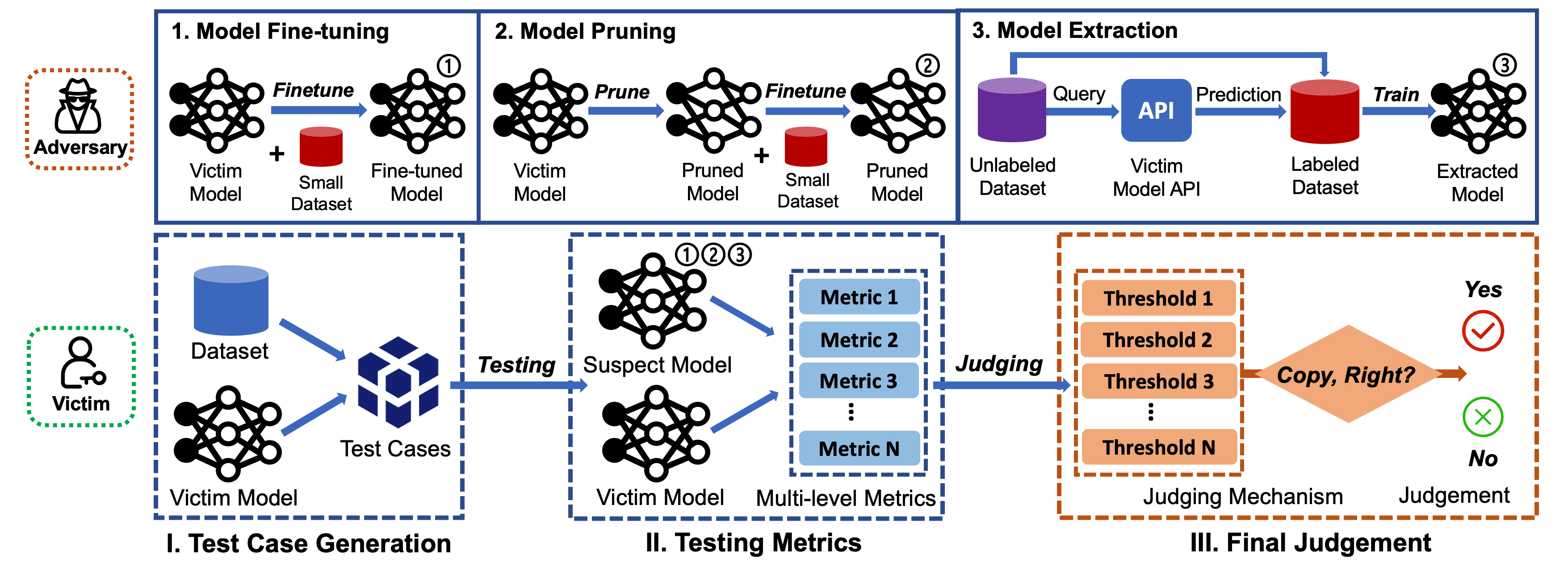
Following the above idea, we design and implement DeepJudge, a novel testing framework for DNN copyright protection. As illustrated in Fig. 1, DeepJudge is composed of three core components. First, we propose a set of multi-level testing metrics to fully characterize a DNN model from different angles. Second, we propose efficient test case generation algorithms to magnify the similarities (or differences) measured by the testing metrics between the two models. Finally, a ‘yes’/‘no’ (stolen copy) judgment will be made for the suspect model based on all similarity scores.

The advantages of DeepJudge include 1) non-invasive: it works directly on the trained models and does not tamper with the training process; 2) efficient: it can be done very efficiently with only a few seed examples and a quick scan of the models; 3) flexible: it can easily incorporate new testing metrics or test case generation methods to obtain more evidence and reliable judgement, and can be applied in both white-box and black-box scenarios with different testing metrics; 4) robust: it is fairly robust to adaptive attacks such as model extraction and defense-aware attacks. The above advantages make DeepJudge a practical, flexible, and extensible tool for copyright protection of deep learning models.

We have implemented DeepJudge as an open-source self-contained toolkit and evaluated DeepJudge on four benchmark datasets (i.e., MNIST, CIFAR-10, ImageNet and Speech Commands) with different DNN architectures, including both convolutional and recurrent neural networks. The results confirm the effectiveness of DeepJudge in providing strong evidence for identifying the stolen copies of a victim model. DeepJudge is also proven to be more robust to a set of adaptive attacks compared to existing defense techniques.

In summary, our main contributions are:

• We propose a novel testing framework DeepJudge for copyright protection of deep learning models. DeepJudge determines whether one model is a copy of the other depending on the similarity scores obtained from a comprehensive set of testing metrics and test case generation algorithms.

• We identify three typical scenarios of model copying including finetuned copy, pruned copy, and extracted copy; define positive and negative suspect models for each scenario; and consider both white-box and black-box protection settings. DeepJudge can produce reliable evidence and judgement to correctly identify the positive suspects across all scenarios and settings.

• DeepJudge is a self-contained open-source tool for robust copyright protection of deep learning models and a strong complement to existing techniques. DeepJudge can be flexibly applied in different DNN copyright protection scenarios and is extensible to new testing metrics and test case generation algorithms.

Figure 1: The overview of DeepJudge Testing Framework.

II Background

II-A Deep Neural Network

A DNN classifier is a decision function $f:X\rightarrow Y$ mapping an input ${\bm{x}}\in X$ to a label $y\in Y=\{1,2,\cdots,C\}$, where $C$ is the total number of classes. It comprises of $L$ layers: $\{f^{1},f^{2},\cdots,f^{L-1},f^{L}\},$ where $f^{1}$ is the input layer, $f^{L}$ is the probability output layer, and $f^{2},\cdots,f^{L-1}$ are the hidden layers. Each layer $f^{l}$ can be denoted by a collection of neurons: $\{n_{l,1},n_{l,2},\cdots,n_{l,N_{l}}\},$ where $N_{l}$ is the total number of neurons at that layer. Each neuron is a computing unit that computes its output by applying a linear transformation followed by a non-linear operation to its input (i.e., output from the precedent layer). We use $\phi_{l,i}({\bm{x}})$ to denote the function that returns the output of neuron $n_{l,i}$ for a given input ${\bm{x}}\in X$. Then, we have the output vector of layer $f^{l}$ ($2\leq l\leq L$): $f^{l}({\bm{x}})=\left\langle\phi_{l,1}({\bm{x}}),\phi_{l,2}({\bm{x}}),\cdots,\phi_{l,N_{l}}({\bm{x}})\right\rangle$. Finally, the output label $f({\bm{x}})$ is computed as $f({\bm{x}})=\operatorname*{arg\,max}f^{L}({\bm{x}})$.

II-B DNN Watermarking

A number of watermarking techniques have been proposed to protect the copyright of DNN models [1, 9, 23, 40, 47, 20]. Similar to traditional multimedia watermarking, DNN watermarking works in two steps: embedding and verification. In the embedding step, the owner embeds a secret watermark (e.g., a signature or a trigger set) into the model during the training process. Depending on how much knowledge of the model is available in the verification step, existing watermarking methods can be broadly categorized into two classes: a) white-box methods for the case when model parameters are available; and b) black-box methods when only predictions of the model can be acquired.

White-box watermarking embeds a pre-designed signature (e.g., a string of bits) into the parameter space of the model via certain regularization terms [9, 40]. The ownership could be claimed when the extracted signature from a suspect model is similar to that of the owner model. Black-box watermarking usually leverages backdoor attacks [16] to implant a watermark pattern into the owner model by training the model with a set of backdoor examples (also known as the trigger set) relabeled to a secret class [23, 47]. The ownership can then be claimed when the defender queries the suspect model for examples attached with the watermark trigger and receives the secret class as predictions.

II-C DNN Fingerprinting

Recently, DNN fingerprinting techniques have been proposed to verify model ownership via two steps: fingerprint extraction and verification. According to the categorization rule for watermarking, fingerprinting methods [2, 27] are all black-box techniques. Moreover, they are non-invasive, which is in sharp contrast with watermarking techniques. Instead of modifying the training procedure to embed identities, fingerprinting directly extracts a unique feature or property of the owner model as its fingerprint (i.e., a unique identifier). The ownership can then be verified if the fingerprint of the owner model matches with that of the suspect model. For example, IPGuard [2] leverages data points close to the classification boundary to fingerprint the boundary property of the owner model. A suspect model is determined to be a stolen copy of the owner model if it predicts the same labels for most boundary data points. [27] proposes a Conferrable Ensemble Method (CEM) to craft conferrable (a subclass of transferable examples) adversarial examples to fingerprint the overlap between two models’ decision boundaries or adversarial subspaces. CEM fingerprinting demonstrates robustness to removal attacks including finetuning, pruning and extraction attacks, except several adapted attacks like adaptive transfer learning and adversarial training [27]. It is the closest work to our DeepJudge. However, as a fingerprinting method, CEM targets uniqueness, while as a testing framework, our DeepJudge targets completeness, i.e., comprehensive characterization of a model with multi-level testing metrics and diverse test case generation methods. Note that CEM fingerprinting can be incorporated into our framework as a black-box metric.

III DNN Copyright Threat Model

We consider a typical attack-defense setting with two parties: the victim and the adversary. Here, the model owner is the victim who trains a DNN model (i.e., the victim model) using private resources. The adversary attempts to steal a copy of the victim model, which 1) mimics its functionality while 2) cannot be easily recognized as a copy. Following this setting, we identify three common threats to DNN copyright: 1) model finetuning, 2) model pruning, and 3) model extraction. The three threats are illustrated in the top row of Fig. 1.

Threat 1: Model Finetuning. In this case, we assume the adversary has full knowledge of the victim model, including model architecture and parameters, and has a small dataset to finetune the model [1, 40]. This occurs, for example, when the victim open-sourced the model for academic purposes only, but the adversary attempts to finetune the model to build commercial products.

Threat 2: Model Pruning. In this case, we also assume the adversary has full knowledge of the victim model’s architecture and parameters. Model pruning adversaries first prune the victim model using some pruning methods, then finetune the model using a small set of data [26, 35].

Threat 3: Model Extraction. In this case, we assume the adversary can only query the victim model for predictions (i.e., the probability vector). The adversary may be aware of the architecture of the victim model but has no knowledge of the training data or model parameters. The goal of model extraction adversaries is to accurately steal the functionality of the victim model through the prediction API [21, 38, 33, 32, 45]. To achieve this, the adversary first obtains an annotated dataset by querying the victim model for a set of auxiliary samples, then trains a copy of the victim model on the annotated dataset. The auxiliary samples can be selected from a public dataset [8, 32] or synthesized using some adaptive strategies [33, 21].

IV Testing for DNN Copyright Protection

In this section, we present DeepJudge, the proposed testing framework that produces supporting evidence to determine whether a suspect model is a copy of a victim model. The victim model can be copied by model finetuning, pruning, or extraction, as discussed in Section III. We identify the following criteria for a reliable copyright protection method:

1. Fidelity. The protection or ownership verification process should not affect the utility of the owner model.

2. Effectiveness. The verification should have high precision and recall in identifying stolen model copies.

3. Efficiency. The verification process should be efficient, e.g., taking much less time than model training.

4. Robustness. The protection should be resilient to adaptive attacks.

DeepJudge is a testing framework designed to satisfy all the above criteria. In the following three subsections, we will first give an overview of DeepJudge, then introduce its multi-level testing metrics and test case generation algorithms.

IV-A DeepJudge Overview

As illustrated in the bottom row of Fig. 1, DeepJudge consists of two components and a final judgement step: i) test case generation, ii) a set of multi-level distance metrics for testing, and iii) a thresholding and voting based judgement mechanism. Alg. 1 depicts the complete procedure of DeepJudge with pseudocode. It takes the victim model $\mathcal{O}$, a suspect model $\mathcal{S}$, and a set of data $\mathcal{D}$ associated with the victim model as inputs and returns the values of the testing metrics as evidence as well as the final judgement. The set of data $\mathcal{D}$ can be provided by the owner from either the training or testing set of the victim model. At the test case generation step, it selects a set of seeds from the input dataset $\mathcal{D}$ (Line 1) and carefully generates a set of extreme test cases from the seeds (Line 2). Based on the test cases generated, DeepJudge computes the distance (dissimilarity) scores defined by the testing metrics between the suspect and victim models (Line 3). The final judgement of whether the suspect is a copy of the victim can be made via a thresholding and voting mechanism according to the dissimilarity scores between the victim and a set of negative suspect models (Line 4).

Input: owner model $\mathcal{O}$, suspect model $\mathcal{S}$, data set $\mathcal{D}$

Output: judgement $\mathcal{J}$, evidence $\mathcal{E}$

// Test case generation (Section IV-C)

1 $Seeds$ $\leftarrow$ SelectSeeds $(\mathcal{O},\mathcal{D})$

2${T}$ $\leftarrow$ GenerateTestCases $(\mathcal{O},Seeds)$

// Testing metrics (Section IV-B)

3 $\mathcal{E}$ $\leftarrow$ ComputeMetrics $(\mathcal{O},\mathcal{S},{T})$

// Final judgement (Section IV-D)

$\mathcal{J}$ $\leftarrow$ Judging $(\mathcal{E})$ // Copy, Right? Yes or No.

4

return $\mathcal{J},\mathcal{E}$

Algorithm 1 $\textsc{DeepJudge}(\mathcal{O},\mathcal{S},\mathcal{D})$

IV-B Multi-level Testing Metrics

We first introduce the testing metrics for two different settings respectively: white-box and black-box. 1) White-box Setting: In this setting, DeepJudge has full access to the internals (i.e., intermediate layer outputs) and the final probability vectors of the suspect model $\mathcal{S}$. 2) Black-box Setting: In this setting, DeepJudge can only query the suspect model $\mathcal{S}$ to obtain the probability vectors or the predicted labels. In both settings, we assume the model owner is willing to provide full access to the victim model $\mathcal{O}$, including the training and test datasets, and the training details if necessary.

TABLE I: Proposed multi-level testing metrics.

Level	Metric	Defense Setting
Property-level	Robustness Distance (RobD)	Black-box
Neuron-level	Neuron Output Distance (NOD)	White-box
	Neuron Activation Distance (NAD)	White-box
Layer-level	Layer Outputs Distance (LOD)	White-box
	Layer Activation Distance (LAD)	White-box
	Jensen-Shanon Distance (JSD)	Black-box

The proposed testing metrics are summarized in Table I, with their suitable defense settings highlighted in the last column. DeepJudge advocates evidence-based ownership verification of DNNs via multi-level testing metrics that complement each other to produce more reliable judgement.

IV-B1 Property-level metrics

There is an abundant set of model properties that could be used to characterize the similarities between two models, such as the adversarial robustness property [11, 4, 2, 27] and the fairness property [30]. Here, we consider the former and define the robustness distance to measure the adversarial robustness discrepancy between two models on the same set of test cases. We will test more properties in our future work.

Denote the function represented by the victim model $\mathcal{O}$ by $f$, given an input ${\bm{x}}_{i}$ and its ground truth label $y_{i}$, an adversarial example ${{\bm{x}}^{\prime}_{i}}$ can be crafted by slightly perturbing ${\bm{x}}_{i}$ towards maximizing the classification error of $f$. This process is known as the adversarial attack, and $f({\bm{x}}^{\prime}_{i})\neq y_{i}$ indicates a successful attack. Adversarial examples can be generated using any existing adversarial attack methods such as FGSM [14] and PGD [28]. Given a set of test cases, we can obtain its adversarial version $T=\{{\bm{x}}^{\prime}_{1},{\bm{x}}^{\prime}_{2},\cdots\}$, where ${\bm{x}}^{\prime}_{i}$ denotes the adversarial example of ${\bm{x}}_{i}$. The robustness property of model $f$ can then be defined as its accuracy on $T$:

$$Rob(f,T)=\frac{1}{|T|}\sum_{i=1}^{|T|}(f({\bm{x}}^{\prime}_{i}))=y_{i}).$$

Robustness Distance (RobD). Let $\hat{f}$ be the suspect model, we define the robustness distance between $f$ and $\hat{f}$ by the absolute difference between the two models’ robustness:

$$RobD(f,\hat{f},T)=|Rob(\hat{f},T)-Rob(f,T)|.$$

The intuition behind RobD is that model robustness is closely related to the decision boundary learned by the model through its unique optimization process, and should be considered as a type of fingerprint of the model. RobD requires minimal knowledge of the model (only its output labels).

IV-B2 Neuron-level metrics

Neuron-level metrics are suitable for white-box testing scenarios where the internal layers’ output of the model is accessible. Intuitively, the output of each neuron in a model follows its own statistical distribution, and the neuron outputs in different models should vary. Motivated by this, DeepJudge uses the output status of neurons to capture the difference between two models and defines the following two neuron-level metrics NOD and NAD.

Neuron Output Distance (NOD). For a particular neuron $n_{l,i}$ with $l$ being the layer index and $i$ being the neuron index within the layer, we denote the neuron output function of the owner’s victim model and the suspect copy model by $\phi_{l,i}$ and $\hat{\phi}_{l,i}$ respectively. NOD measures the average neuron output difference between the two models over a given set $T=\{{\bm{x}}_{1},{\bm{x}}_{2},\cdots\}$ of test cases:

$$NOD(\phi_{l,i},\hat{\phi}_{l,i},T)=\frac{1}{|T|}\sum_{{\bm{x}}\in T}|\phi_{l,i}({\bm{x}})-\hat{\phi}_{l,i}({\bm{x}})|.$$

Neuron Activation Distance (NAD). Inspired by the Neuron Coverage [34] for testing deep learning models, NAD measures the difference in activation status (‘activated’ vs. ‘not activated’) between the neurons of two models. Specifically, for a given test case ${\bm{x}}\in T$, the neuron $n_{l,i}$ is determined to be ‘activated’ if its output value $\phi_{l,i}({\bm{x}})$ is larger than a pre-specified threshold. The NAD between the two models with respect to neuron $n_{l,i}$ can then be calculated as:

$$NAD(\phi_{l,i},\hat{\phi}_{l,i},T)=\frac{1}{|T|}\sum_{{\bm{x}}\in T}|S({\phi_{l,i}({\bm{x}})})-S({\hat{\phi}_{l,i}({\bm{x}})})|,$$

where the step function $S(\phi_{l,i}({\bm{x}}))$ returns $1$ if $\phi_{l,i}({\bm{x}})$ is greater than a certain threshold, $0$ otherwise.

IV-B3 Layer-level metrics

The layer-wise metrics in DeepJudge take into account the output values of the entire layer in a DNN model. Compared with neuron-level metrics, layer-level metrics provide a full-scale view of the intermediate layer output difference between two models.

Layer Output Distance (LOD). Given a layer index $l$, let $f^{l}$ and $\hat{f}^{l}$ represent the layer output functions of the victim model and the suspect model, respectively. LOD measures the $L^{p}$-norm distance between the two models’ layer outputs:

$$LOD(f^{l},\hat{f}^{l},T)=\frac{1}{|T|}\sum_{{\bm{x}}\in T}||f^{l}({\bm{x}})-\hat{f}^{l}({\bm{x}})||_{p},$$

where $||\cdot||_{p}$ denotes the $L^{p}$-norm ($p=2$ in our experiments).

Layer Activation Distance (LAD). LAD measures the average NAD of all neurons within the same layer:

$$LAD(f^{l},\hat{f}^{l},T)=\frac{1}{|N_{l}|}\sum_{i=1}^{|N_{l}|}NAD(\phi_{l,i},\hat{\phi}_{l,i},T),$$

where $N_{l}$ is the total number of neurons at the $l$-th layer, and $\phi_{l,i}$ and $\hat{\phi}_{l,i}$ are the neuron output functions from $f^{l}$ and $\hat{f}^{l}$.

Jensen-Shanon Distance (JSD). JSD [13] is a metric that measures the similarly of two probability distributions, and a small JSD value implies the two distributions are very similar. Let $f^{L}$ and $\hat{f}^{L}$ denote the output functions (output layer) of the victim model and the suspect model, respectively. Here, we apply JSD to the output layer as follows:

$$JSD(f^{L},\hat{f}^{L},T)=\frac{1}{2|T|}\sum_{{\bm{x}}\in T}K(f^{L}({\bm{x}}),q)+K(\hat{f}^{L}({\bm{x}}),q),$$

where $q=(f^{L}({\bm{x}})+\hat{f}^{L}({\bm{x}}))/2$ and $K(\cdot,\cdot)$ is the Kullback-Leibler divergence. JSD quantifies the similarity between two models’ output distributions, and is particularly more powerful against model extraction attacks where the suspect model is extracted based on the probability vectors (distributions) returned by the victim model.

IV-C Test Case Generation

To fully exercise the testing metrics defined above, we need to magnify the similarities between a positive suspect and the victim model, while minimizing the similarities of a negative suspect to the victim model. In DeepJudge, this is achieved by smart test case generation methods. Meanwhile, test case generation should respect the model accessibility in different defense settings, i.e., black-box vs. white-box.

IV-C1 Black-box setting

Figure 2: DeepJudge uses adversarial examples of the victim model to probe the difference in models’ decision boundary.

When only the input and output of a suspect model are accessible, we populate the test set $T$ using adversarial inputs generated by existing adversarial attack methods on the victim model. We consider three widely used adversarial attack methods, including Fast Gradient Sign Method (FGSM) [14], Projected Gradient Descent (PGD) [28], and Carlini & Wagner’s (CW) attack [4], where FGSM and PGD are $L^{\infty}$-bounded adversarial methods, and CW is an $L^{2}$-bounded attack method. This gives us more diverse test cases with both $L^{\infty}$- and $L^{2}$-norm perturbed adversarial test cases. The detailed description and exact parameters used for adversarial test case generation are provided in Appendix A-D.

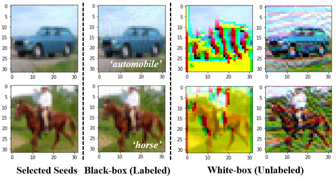
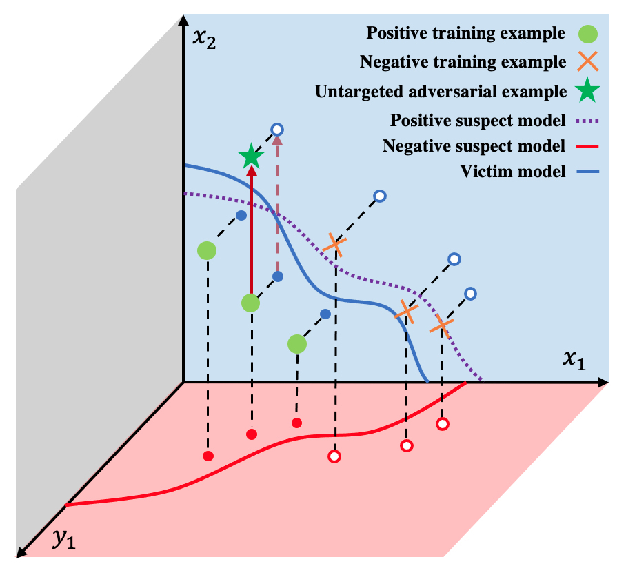
Fig. 2 illustrates the rationale behind using adversarial examples as test cases. Finetuned and pruned model copies are directly derived from the victim model, thus they share similar decision boundaries (purple line) as the victim model. However, the negative suspect models are trained from scratch on different data or with different initializations, thus having minimum or no overlapping with the victim model’s decision boundary. By subverting the model’s predictions, adversarial examples cross the decision boundary from one side to the other (we use untargeted adversarial examples). Although the extracted models by model extraction attacks are trained from scratch by the adversary, the training relies on the probability vectors returned by the victim model, which contains information about the decision boundary. This implies that the extracted model will gradually mimic the decision boundary of the victim model. From this perspective, the decision boundary (or robustness) based testing imposes a dilemma to model extraction adversaries: the better the extraction, the more similar the extracted model to the victim model, and the easier it to be identified by our decision boundary based testing.

IV-C2 White-box setting

In this case, the internals of the suspect model are accessible, thus a more fine-grained approach for test case generation becomes feasible. As shown in Fig. 3, given a seed input and a specified layer, DeepJudge generates one test case for each neuron, and the corner case of the neuron’s activation is of our particular interest.

Figure 3: DeepJudge tests each neuron and generates a test case to explore the corner region of its output distribution.

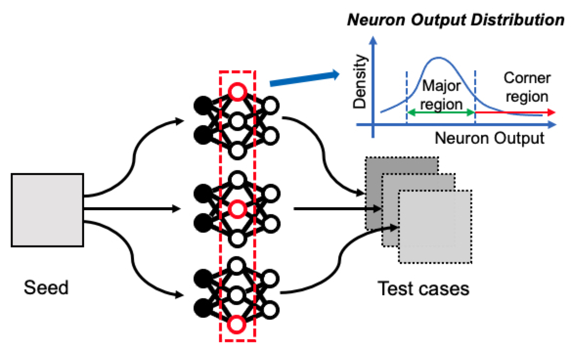
The test generation algorithm is described in Alg. 2. It takes the owner’s victim model $\mathcal{O}$ and a set of selected seeds $Seeds$ as input, and returns the set of generated test cases $T$. $T$ is initialized to be empty (Line 1). The main content of the algorithm is a nested loop (Lines 2-13), in which for each neuron $n_{l,i}$ required by the metrics in Section IV-B, the algorithm searches for an input that activates the neuron’s output $\phi_{l,i}({\bm{x}}^{\prime})$ more than a threshold value. At each outer loop iteration, an input is sampled from the $Seeds$ (Lines 3-4). It is then iteratively perturbed in the inner loop following the neuron activation’s gradient update (Lines 6-7), until an input ${\bm{x}}^{\prime}$ that can satisfy the threshold condition is found and is added into the test suite $T$ (Lines 8-11) or when the maximum number of iterations is reached. The parameter $lr$ (Line 7) is used to control that the search space of the input with perturbation is close enough to its seed input. Finally, the generated test suite $T$ is returned.

We discuss how to configure the specific threshold $k$ for a neuron $n_{l,i}$ used in Alg. 2. Since the statistics may vary across different neurons, we pre-compute the threshold $k$ based on the training data and the owner model, which is the maximum value (upper bound) of the corresponding neuron output over all training samples. The final threshold value is then adjusted by a hyper-parameter $m$ to be used in Alg. 2 for more reasonable and adaptive thresholds. Note that the thresholds for all interested neurons can be calculated once by populating layer by layer across the model.

Input: owner model $\mathcal{O}$, a set of seed inputs $Seeds$

Output: test suite $T$

1 Initialize test suite $T\leftarrow\emptyset$

2for each neuron $n_{l,i}$ do

3      

4      Sample a seed input ${\bm{x}}\leftarrow$ $Seeds.choice()$

5      ${\bm{x}}^{\prime}\leftarrow copy({\bm{x}})$

6      for $iter=1$ to $iters$ do

7            

8            Calculate gradients $grads\leftarrow\frac{\nabla\phi_{l,i}({\bm{x}}^{\prime})}{\nabla{\bm{x}}^{\prime}}$

9            Perturb input ${\bm{x}}^{\prime}\leftarrow{\bm{x}}^{\prime}+lr\cdot grads$

10            if $\phi_{l,i}({\bm{x}}^{\prime})>$ threshold $k$ then

11                   Add new test case $T\leftarrow T\cup\{{\bm{x}}^{\prime}\}$

12                   break

13             end if

14            

15       end for

16      

17 end for

return $T$

Algorithm 2 GenerateTestCases($\mathcal{O}$, $Seeds$)

IV-D Final Judgement

The judgment mechanism of DeepJudge has two steps: thresholding and voting. The thresholding step determines a proper threshold for each testing metric based on the statistics of a set of negative suspect models (see Section V-A3 for more details). The voting step examines a suspect model against each testing metric, and gives it a positive vote if its distance to the victim model is lower than the threshold of that metric. The lower a measured metric value, the more likely the suspect model is a copy of the victim, according to this metric. The final judgment can then be made based on the votes: the suspect model will be identified as a positive suspect if it receives more positive votes, and a negative suspect otherwise.

For each testing metric $\lambda$, we set the threshold adaptively using an $\varepsilon$-difference strategy. Specifically, we use one-tailed T-test to calculate the lower bound $LB_{\lambda}$ based on the statistics of the negative suspect models at the 99% confidence level. If the measured difference $\lambda(\mathcal{O},\mathcal{S},T)$ is lower than $LB_{\lambda}$, $\mathcal{S}$ will be a copy of $\mathcal{O}$ with high probability. The threshold for each metric $\lambda$ is defined as: $\tau_{\lambda}=\alpha_{\lambda}\cdot LB_{\lambda}$, where $\alpha_{\lambda}$ is a user-specified relaxing parameter controlling the sensitivity of the judgement. As $\alpha_{\lambda}$ decreases, the false positive rate (the possibility of misclassifying a negative suspect as a stolen copy) will also increase. We empirically set $\alpha=0.9$ for black-box metrics and $\alpha=0.6$ for white-box metrics respectively, depending on the negative statistics.

DeepJudge makes the final judgement by voting below:

$$p_{copy}(\mathcal{O},\mathcal{S},T)=\frac{1}{|\Lambda|}\sum_{\lambda\in\Lambda}\mathbbm{1}\big{(}\lambda(\mathcal{O},\mathcal{S},T)\leq\tau_{\lambda}\big{)},$$

where $\mathbbm{1}$ in the indicator function and $\Lambda$ denotes the set of DeepJudge testing metrics, i.e., {RobD, NOD, NAD, LOD, LAD, JSD}. Note that, depending on the defense setting (white-box vs. black-box), only a subset of the testing metrics can be applied and the averaging can only be applied on the available metrics. DeepJudge identifies a positive suspect copy if $p_{copy}$ is larger than 0.5 and a negative one otherwise. Arguably, voting is the most straightforward way of making the final judgement. While this simple voting strategy works reasonably well in our experiments, we believe more advanced judgement rules can be developed for diverse real-world protection scenarios.

IV-E DeepJudge vs. Watermarking & Fingerprinting

TABLE II: A comparison of different copyright protection methods.

Method	Type	Non-invasive	Evaluated Settings		Evaluated Attacks
			Black-box	White-box	Finetuning	Pruning	Extraction
Uchida et al. [40]	Watermarking	✗	✗	✓	✓	✓	✗
Merrer et al. [23]	Watermarking	✗	✓	✗	✓	✓	✗
Adi et al. [1]	Watermarking	✗	✓	✗	✓	✗	✗
Zhang et al. [47]	Watermarking	✗	✓	✗	✓	✓	✗
Darvish et al. [9]	Watermarking	✗	✓	✓	✓	✓	✗
Jia et al. [20]	Watermarking	✗	✓	✗	✓	✓	✓
Cao et al. [2]	Fingerprinting	✓	✓	✗	✓	✓	✗
Lukas et al. [27]	Fingerprinting	✓	✓	✗	✓	✓	✓
DeepJudge (Ours)	Testing	✓	✓	✓	✓	✓	✓

Here, we briefly discuss why our testing approach is more favorable in certain settings and how it complements existing defense techniques. Table II summarizes the differences of DeepJudge to existing watermarking and fingerprinting methods, from three aspects: 1) whether the method is non-invasive (i.e., independent of model training); 2) whether it is particularly designed for or evaluated in different defense settings (i.e., white-box vs. black-box); and 3) whether the method is evaluated against different attacks (i.e., finetuning, pruning and extraction). DeepJudge is training-independent, able to be flexibly applied in either white-box or black-box settings, and evaluated (also proven to be robust) against all three types of common copyright attacks including model finetuning, pruning and extraction, with empirical evaluations and comparisons deferred to Section V-B3.

Watermarking is invasive (training-dependent), whereas fingerprinting and testing are non-invasive (training independent). The effectiveness of watermarking depends on how well the owner model memorizes the watermark and how robust the memorization is to different attacks. While watermarking can be robust to finetuning or pruning attacks [40, 47], it is particularly vulnerable to the emerging model extraction attack (see Section V-C2). This is because model extraction attacks only extract the key functionality of the model, however, watermarks are often task-irrelevant. Despite the above weaknesses, watermarking is the only technique that can embed the owner identity/signature into the model, which is beyond the functionalities of fingerprinting or testing.

Fingerprinting shares certain similarities with testing. However, they differ in their goals. Fingerprinting aims for “uniqueness”, i.e., a unique fingerprint of the model, while testing aims for “completeness”, i.e., to test as many dimensions as possible to characterize not only the unique but also the common properties of the model. Arguably, effective fingerprints are also valid black-box testing metrics. But as a testing framework, our DeepJudge is not restricted to a particular metric or test case generation method. Our experiments in Section VI show that a single metric or fingerprint is not sufficient to handle the diverse and adaptive model stealing attacks. In Section VI-B, we will also show that our DeepJudge can survive those adaptive attacks that break fingerprinting by dynamically changing the test case generation strategy. We anticipate a long-running arms race in deep learning copyright protection between model owners and adversaries, where watermarking, fingerprinting and testing methods are all important for a comprehensive defense.

V Experiments

We have implemented DeepJudge as a self-contained toolkit in Python. In the following, we first evaluate the performance of DeepJudge against model finetuning and model pruning (Section V-B), which are two threat scenarios extensively studied by watermarking methods [1, 9]. We then examine DeepJudge against more challenging model extraction attacks in Section V-C. Finally, we test the robustness of DeepJudge under adaptive attacks in Section VI. Overall, we evaluated DeepJudge with 11 attack methods, 3 baselines, and over 300 deep learning models trained on 4 datasets.

V-A Experimental Setup

V-A1 Datasets & Victim Models

We run the experiments on three image classification datasets (i.e., MNIST [24], CIFAR-10 [22] and ImageNet [36]) and one audio recognition dataset (i.e., SpeechCommands [42]). The models used for the four datasets are summarized in Table III, including three convolutional architectures and one recurrent neural network. For each dataset, we divide the training data into two subsets. The first subset (50% of the training examples) is used to train the victim model. More detailed experimental settings can be found in Appendix A-A.

V-A2 Positive suspect models

Positive suspect models are derived from the victim models via finetuning, pruning, or model extraction. These models are considered as stolen copies of the owner’s victim model. DeepJudge should provide evidence for the victim to claim ownership.

V-A3 Negative suspect models

Negative suspect models have the same architecture as the victim models but are trained independently using either the remaining 50% of training data or the same data but with different random initializations. The negative suspect models serve as the control group to show that DeepJudge will not claim wrong ownership. These models are also used to compute the testing thresholds ($\tau$). The same training pipeline and the setting are used to train the negative suspect models. Specifically, “Neg-1” are trained with different random initializations while “Neg-2” are trained using a separate dataset (the other 50% of training samples).

V-A4 Seed selection

Seed selection prepares the $Seeds$ examples used to generate the test cases. Here, we apply the sampling strategy used in DeepGini [12] to select a set of high-confidence seeds from the test dataset (details are in Appendix A-B). The intuition is that high-confidence seeds are well-learned by the victim model, thus carrying more unique features of the victim model. More adaptive seed selection strategies are explored in the adaptive attack section VI-B1.

V-A5 Adversarial example generation

We use three classic attacks including FGSM [14], PGD [28] and CW [4] to generate adversarial test cases as introduced in Section IV-C1.

TABLE III: Datasets and victim models.

Dataset	Type	Model	#Params	Accuracy
MNIST	Image	LeNet-5	107.8 K	98.5%
CIFAR-10	Image	ResNet-20	274.4 K	84.8%
ImageNet	Image	VGG-16	33.65 M	74.4%
SpeechCommands	Audio	LSTM(128)	132.4 K	94.9%
#Params: number of parameters

V-B Defending Against Model Finetuning & Pruning

As model finetuning and pruning threats are similar in processing the victim model (see Section III), we discuss them together here. These two are also the most extensively studied threats in prior watermarking works [1, 40].

V-B1 Attack strategies

Given a victim model and a small set of data in the same task domain, we consider the following four commonly used model finetuning & pruning strategies: a) Finetune the last layer (FT-LL). Update the parameters of the last layer while freezing all other layers. b) Finetune all layers (FT-AL). Update the parameters of the entire model. c) Retrain all layers (RT-AL). Re-initialize the parameters of the last layer then update the parameters of the entire model. d) Parameter pruning (P-r%). Prune $r$ percentage of the parameters that have the smallest absolute values, then finetune the pruned model to restore the accuracy. We test both low ($r$=$20\%$) and high ($r$=$60\%$) pruning rates. Typical data-augmentations are also used to strengthen the attacks. More details of these attacks are in Appendix A-C.

TABLE IV: Performance of DeepJudge against model finetuning and pruning attacks in the black-box setting. PGD [28] is used to generate the adversarial test cases. ACC is the validation accuracy. For each metric, the values below (indicating ‘copy’) or above (indicating ‘not copy’) the threshold $\tau_{\lambda}$ (the last row) are highlighted in red (copy alert) and green (no alert), respectively. ‘Yes (2/2)’: two of the metrics vote for ‘copy’ ($p_{copy}=100\%$); ‘No (0/2)’: none of the metrics vote for ‘copy’ ($p_{copy}=0\%$).

Model Type		MNIST				CIFAR-10
		ACC	RobD	JSD	Copy?	ACC	RobD	JSD	Copy?
Victim Model		98.5%	–	–	–	84.8%	–	–	–
Positive Suspect Models	FT-LL	98.8$\pm$0.0%	0.019$\pm$0.003	0.016$\pm$0.002	Yes (2/2)	82.1$\pm$0.1%	0.000$\pm$0.000	0.002$\pm$0.001	Yes (2/2)
	FT-AL	98.7$\pm$0.1%	0.045$\pm$0.016	0.033$\pm$0.010	Yes (2/2)	79.9$\pm$1.4%	0.192$\pm$0.028	0.162$\pm$0.014	Yes (2/2)
	RT-AL	98.4$\pm$0.2%	0.298$\pm$0.039	0.151$\pm$0.017	Yes (2/2)	79.4$\pm$0.8%	0.237$\pm$0.055	0.197$\pm$0.027	Yes (2/2)
	P-20%	98.7$\pm$0.1%	0.058$\pm$0.014	0.035$\pm$0.009	Yes (2/2)	81.7$\pm$0.2%	0.155$\pm$0.032	0.128$\pm$0.018	Yes (2/2)
	P-60%	98.6$\pm$0.1%	0.172$\pm$0.024	0.097$\pm$0.010	Yes (2/2)	81.1$\pm$0.6%	0.318$\pm$0.036	0.233$\pm$0.019	Yes (2/2)
Negative Suspect Models	Neg-1	98.4$\pm$0.3%	0.968$\pm$0.014	0.614$\pm$0.016	No (0/2)	84.2$\pm$0.6%	0.920$\pm$0.021	0.603$\pm$0.016	No (0/2)
	Neg-2	98.3$\pm$0.2%	0.949$\pm$0.029	0.600$\pm$0.020	No (0/2)	84.9$\pm$0.5%	0.926$\pm$0.030	0.615$\pm$0.021	No (0/2)
	$\tau_{\lambda}$	–	0.852	0.538	–	–	0.816	0.537	–

Model Type		ImageNet				SpeechCommands
		ACC	RobD	JSD	Copy?	ACC	RobD	JSD	Copy?
Victim model		74.4%	–	–	–	94.9%	–	–	–
Positive Suspect Models	FT-LL	73.2$\pm$0.4%	0.034$\pm$0.007	0.009$\pm$0.003	Yes (2/2)	95.2$\pm$0.1%	0.104$\pm$0.007	0.036$\pm$0.006	Yes (2/2)
	FT-AL	70.8$\pm$0.9%	0.073$\pm$0.011	0.043$\pm$0.011	Yes (2/2)	95.8$\pm$0.3%	0.326$\pm$0.024	0.155$\pm$0.014	Yes (2/2)
	RT-AL	53.3$\pm$0.8%	0.192$\pm$0.008	0.251$\pm$0.015	Yes (2/2)	94.3$\pm$0.3%	0.445$\pm$0.019	0.231$\pm$0.016	Yes (2/2)
	P-20%	69.7$\pm$1.1%	0.106$\pm$0.010	0.064$\pm$0.003	Yes (2/2)	95.4$\pm$0.2%	0.310$\pm$0.026	0.152$\pm$0.013	Yes (2/2)
	P-60%	68.8$\pm$1.0%	0.161$\pm$0.017	0.091$\pm$0.004	Yes (2/2)	95.0$\pm$0.5%	0.437$\pm$0.030	0.215$\pm$0.013	Yes (2/2)
Negative Suspect Models	Neg-1	74.2$\pm$0.3%	0.737$\pm$0.007	0.395$\pm$0.006	No (0/2)	94.9$\pm$0.7%	0.819$\pm$0.025	0.456$\pm$0.014	No (0/2)
	Neg-2	73.9$\pm$0.5%	0.760$\pm$0.010	0.429$\pm$0.004	No (0/2)	94.5$\pm$0.8%	0.832$\pm$0.024	0.472$\pm$0.012	No (0/2)
	$\tau_{\lambda}$	–	0.659	0.356	–	–	0.727	0.405	–

TABLE V: Performance of DeepJudge against model finetuning and pruning attacks in the white-box setting. Algorithm 2 is used to generate the test cases. For each metric, the values below (indicating ‘copy’) or above (indicating ‘not copy’) the threshold $\tau_{\lambda}$ (the last row) are highlighted in red (copy alert) and green (no alert) respectively. ‘Yes (4/4)’: all 4 metrics vote for ‘copy’ ($p_{copy}=100\%$); ‘No (0/4)’: none of the metrics vote for ‘copy’ ($p_{copy}=0\%$).

Model Type		MNIST					CIFAR-10
		NOD	NAD	LOD	LAD	Copy?	NOD	NAD	LOD	LAD	Copy?
Positive Suspect Models	FT-LL	0.00$\pm$0.00	0.00$\pm$0.00	0.00$\pm$0.00	0.00$\pm$0.00	Yes (4/4)	0.00$\pm$0.00	0.00$\pm$0.00	0.00$\pm$0.00	0.00$\pm$0.00	Yes (4/4)
	FT-AL	0.08$\pm$0.01	0.23$\pm$0.21	0.32$\pm$0.03	0.82$\pm$0.16	Yes (4/4)	0.15$\pm$0.02	0.30$\pm$0.12	0.74$\pm$0.07	0.21$\pm$0.04	Yes (4/4)
	RT-AL	0.31$\pm$0.02	0.37$\pm$0.20	0.97$\pm$0.04	1.27$\pm$0.29	Yes (4/4)	0.18$\pm$0.02	0.26$\pm$0.10	0.78$\pm$0.03	0.22$\pm$0.02	Yes (4/4)
	P-20%	0.10$\pm$0.01	0.16$\pm$0.12	0.36$\pm$0.03	0.79$\pm$0.15	Yes (4/4)	0.28$\pm$0.03	0.32$\pm$0.09	0.77$\pm$0.06	0.24$\pm$0.02	Yes (4/4)
	P-60%	0.11$\pm$0.01	0.82$\pm$0.26	0.43$\pm$0.03	1.16$\pm$0.08	Yes (4/4)	0.62$\pm$0.03	1.65$\pm$0.34	2.80$\pm$0.21	0.93$\pm$0.10	Yes (4/4)
Negative Suspect Models	Neg-1	0.77$\pm$0.07	11.46$\pm$1.14	1.73$\pm$0.06	6.42$\pm$0.84	No (0/4)	3.09$\pm$0.30	10.94$\pm$1.74	11.85$\pm$1.01	5.41$\pm$0.67	No (0/4)
	Neg-2	0.79$\pm$0.08	12.28$\pm$1.50	1.78$\pm$0.13	6.37$\pm$0.47	No (0/4)	3.21$\pm$0.18	11.09$\pm$0.71	12.60$\pm$1.33	5.37$\pm$0.72	No (0/4)
	$\tau_{\lambda}$	0.45	6.74	1.03	3.65	–	1.79	6.14	6.89	3.01	–

Model Type		ImageNet					SpeechCommands
		NOD	NAD	LOD	LAD	Copy?	NOD	NAD	LOD	LAD	Copy?
Positive Suspect Models	FT-LL	0.00$\pm$0.00	0.00$\pm$0.00	0.00$\pm$0.00	0.00$\pm$0.00	Yes (4/4)	0.000$\pm$0.000	0.00$\pm$0.00	0.00$\pm$0.00	0.000$\pm$0.00	Yes (4/4)
	FT-AL	0.02$\pm$0.01	0.18$\pm$0.09	0.16$\pm$0.05	0.58$\pm$0.13	Yes (4/4)	0.037$\pm$0.003	0.05$\pm$0.02	0.42$\pm$0.02	12.82$\pm$1.00	Yes (4/4)
	RT-AL	0.03$\pm$0.00	0.30$\pm$0.07	0.25$\pm$0.03	0.78$\pm$0.05	Yes (4/4)	0.055$\pm$0.003	0.25$\pm$0.31	0.64$\pm$0.08	21.64$\pm$2.47	Yes (4/4)
	P-20%	0.11$\pm$0.01	0.83$\pm$0.06	0.76$\pm$0.01	1.67$\pm$0.22	Yes (4/4)	0.038$\pm$0.002	0.03$\pm$0.02	0.44$\pm$0.02	14.57$\pm$3.12	Yes (4/4)
	P-60%	0.77$\pm$0.01	3.09$\pm$0.12	3.41$\pm$0.03	6.63$\pm$0.23	Yes (4/4)	0.094$\pm$0.004	0.45$\pm$0.32	0.67$\pm$0.04	20.58$\pm$3.44	Yes (4/4)
Negative Suspect Models	Neg-1	6.55$\pm$0.78	32.18$\pm$2.97	35.03$\pm$3.13	30.32$\pm$1.91	No (0/4)	0.488$\pm$0.013	39.61$\pm$9.74	2.82$\pm$0.08	64.32$\pm$2.42	No (0/4)
	Neg-2	6.25$\pm$0.39	30.04$\pm$2.44	44.21$\pm$3.11	29.58$\pm$0.86	No (0/4)	0.480$\pm$0.012	34.84$\pm$6.07	2.79$\pm$0.09	62.69$\pm$1.75	No (0/4)
	$\tau_{\lambda}$	3.48	17.17	20.74	17.20	–	0.286	19.77	1.66	37.48	–

V-B2 Effectiveness of DeepJudge

The results are presented separately for black-box vs. white-box settings.

Black-box Testing. In this setting, only the output probabilities of the suspect model are accessible. Here, DeepJudge uses the two black-box metrics: RobD and JSD. For both metrics, the smaller the value, the more similar the suspect model is to the victim model. Table IV reports the results of DeepJudge on the four datasets. Note that we randomly repeat the experiment 6 times for each finetuning or pruning attack and 12 times for independent training (as more negative suspect models will result in a more accurate judging threshold). Then, we report the average and standard deviation (in the form of $a\pm b$) in each entry of Table IV. Clearly, all positive suspect models are more similar to the victim model with significantly smaller RobD and JSD values than negative suspect models. Specifically, a low RobD value indicates that the adversarial examples generated on the victim model have a high transferability to the suspect model, i.e., its decision boundary is closer to the victim model. In contrast, the RobD values of the negative suspect models are much larger than that of the positives, which matches our intuition in Fig. 2.

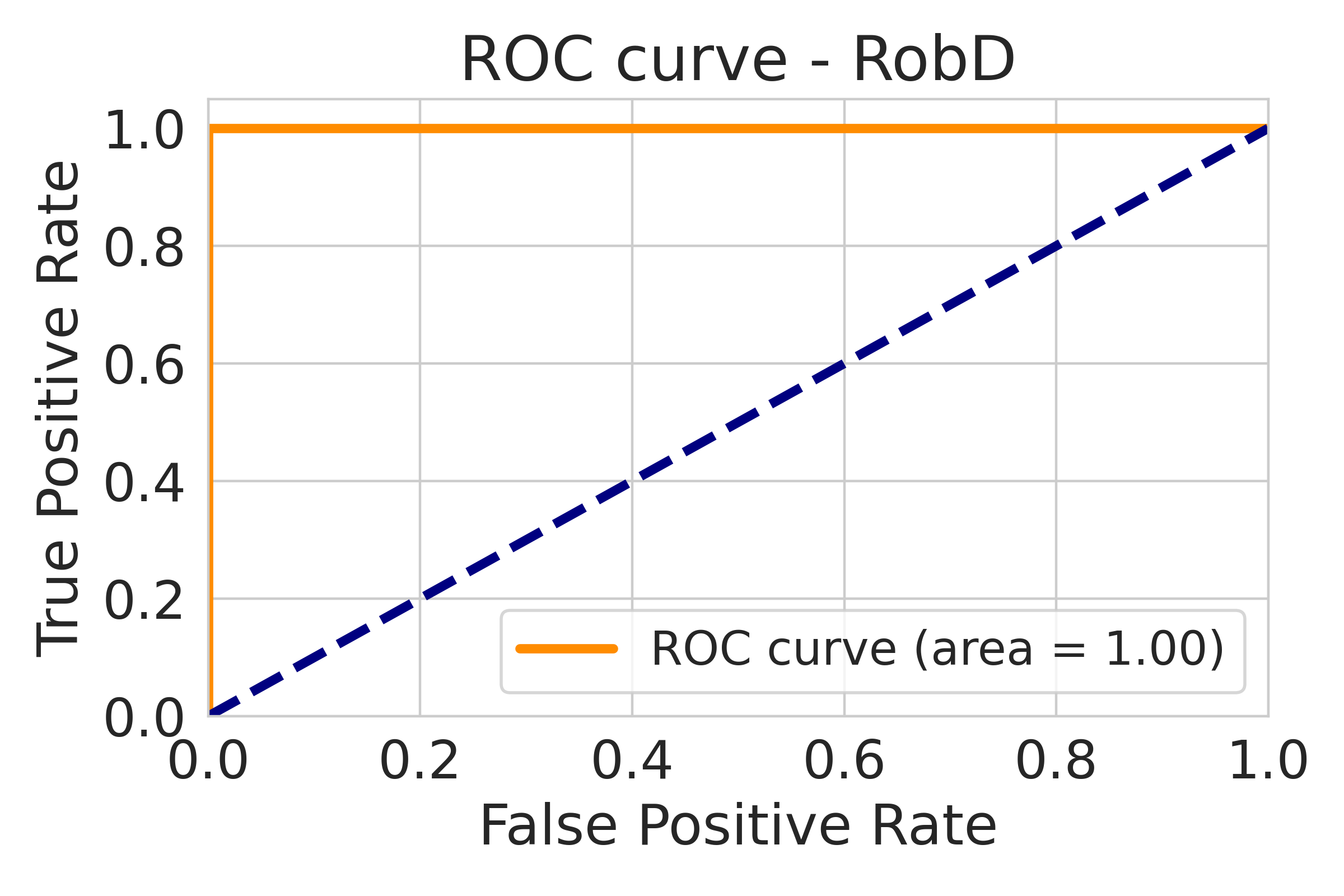
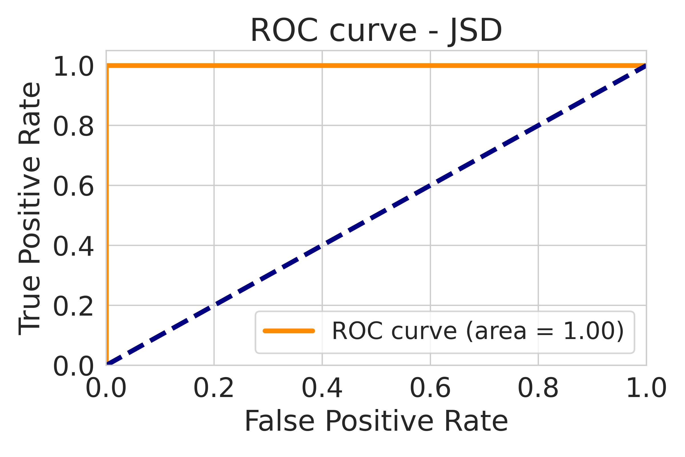
To further confirm the effectiveness of the proposed metrics, we show the ROC curve for a total of 54 models (30 positive suspect models and 24 negative suspect models) for RobD and JSD in Figure 4. The AUC values are 1 for both metrics. Note that we omit the plots for the following white-box testing as the AUC values for all metrics are also 1.

White-box Testing. In this setting, all intermediate-layer outputs of the suspect model are accessible. DeepJudge can thus use the four white-box metrics (i.e., NOD, NAD, LOD, and LAD) to test the models. Table V reports the results on the four datasets. Similar to the two black-box metrics, the smaller the white-box metrics, the more likely the suspect model is a stolen copy. As shown in Table V, there is a fundamental difference between the two sets (positive vs. negative) of suspect models according to each of the four metrics. That is, the two sets of models are completely separable, leading to highly accurate detection of the positive copies. It is not surprising as white-box testing can collect more fine-grained information from the suspect models. In both the black-box and white-box settings, the voting in DeepJudge overwhelmingly supports the correct final judgement (the ‘Copy?’ column).

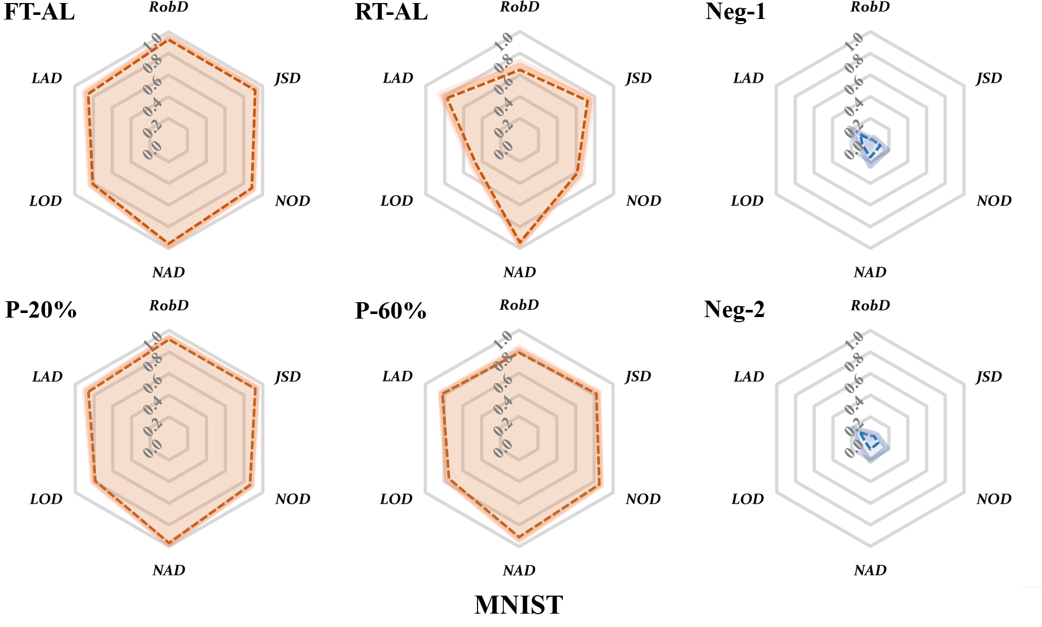
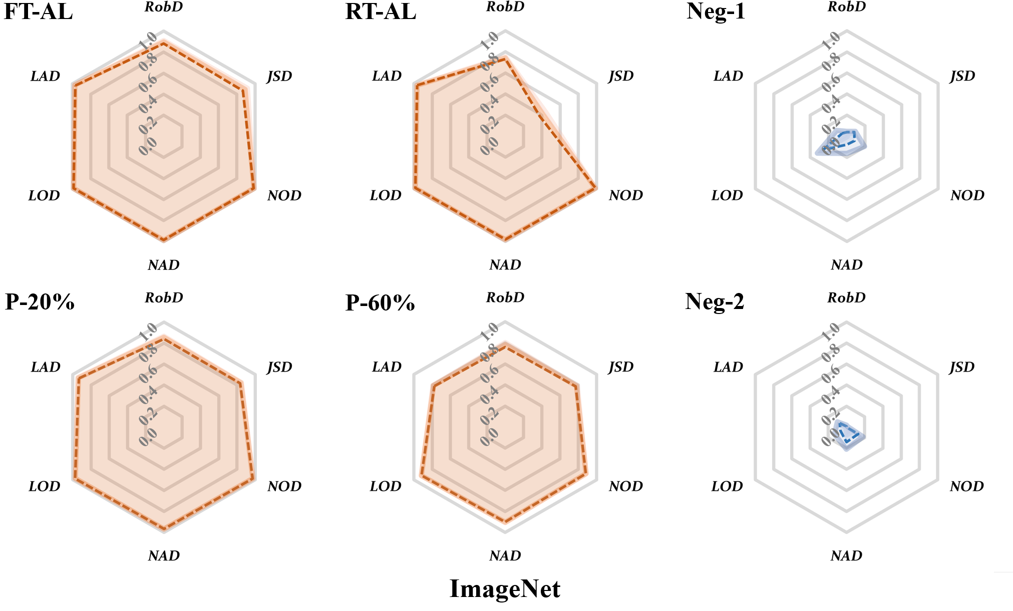
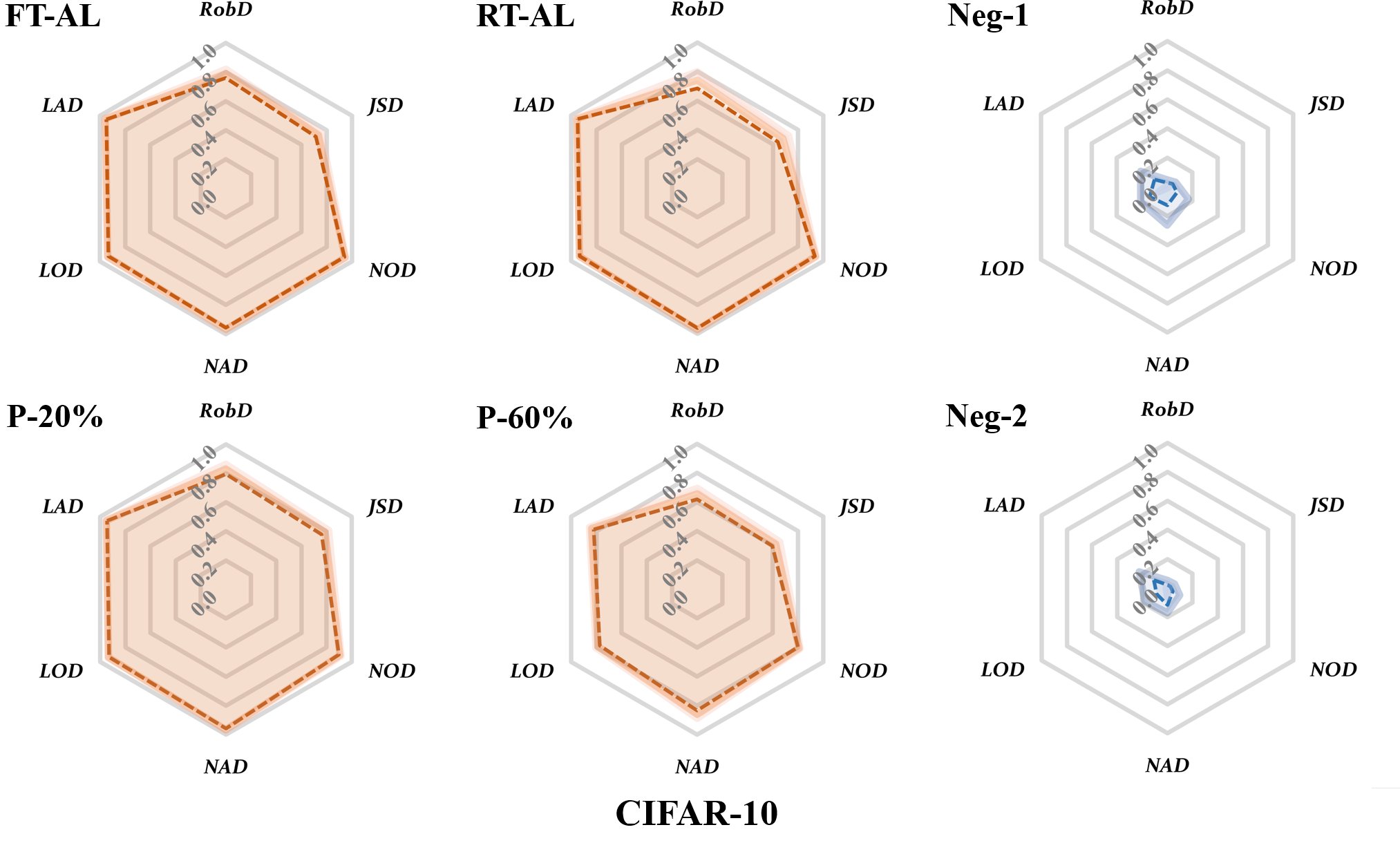
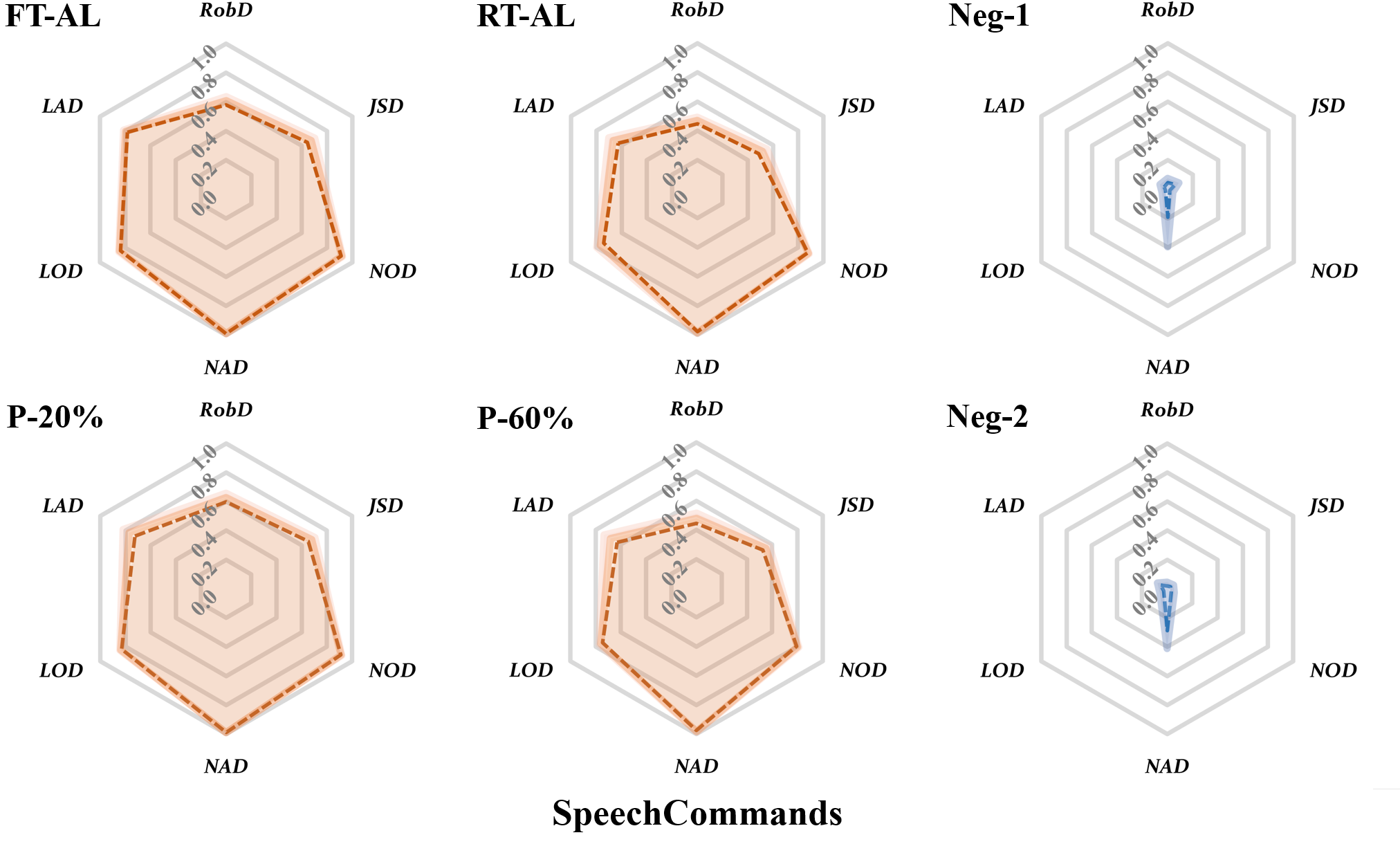
Combined Visualization. To better understand the power of DeepJudge, we combine the black-box and white-box testing results for each suspect model into a single radar chart in Fig. 5. Each dimension of the radar chart corresponds to a similarity score given by one testing metric. For better visual effect, we normalize the values of the testing metrics into the range $[0,1]$, and the larger the normalized value, the more similar the suspect model to the victim. Thus, the filled area could be viewed as the accumulated supporting evidence by DeepJudge metrics for determining whether the suspect model is a stolen copy. Clearly, DeepJudge is able to accurately distinguish positive suspects from negative ones. Among the positive suspect models, the areas of RT-AL and P-60% are noticeably smaller than the other two, meaning they are harder to detect. This is because these two attacks make the most parameter modifications to the victim model. Comparing the metrics, activation-based metrics (e.g., NAD) demonstrate better performance than output-based metrics (e.g., NOD), while white-box metrics are stronger than black-box metrics, especially against strong attacks like RT-AL. In Appendix A-D, we also analyze the influencing factors including adversarial test case generation and layer selection (for computing the testing metrics) via several calibration experiments. An analysis of how different levels of finetuning or pruning affect DeepJudge is presented in Appendix A-H.

Time Cost of DeepJudge. The time cost of generating test cases using 1k seeds is provided in appendix Table IX. For the black-box setting, we report the cost of PGD-based generation, while for the white-box setting, we report that of Algorithm 2. It shows that the time cost of white-box generation is slightly higher but is still very efficient in practice. The maximum time cost occurs on the SpeechCommands dataset for white-box generation, which is $\sim 1.2$ hours. This time cost is regarded as efficient since test case generation is a one-time effort, and the additional time cost of scanning a suspect model with the test cases is almost negligible.

Figure 4: The detection ROC curves of metrics RobD and JSD on CIFAR-10 suspect models, and $AUC=1$ for both metrics.

Figure 5: Similarities of different suspect models to the victim model on CIFAR-10 (left 3 columns) and SpeechCommands (right 3 columns). We use the orange line for the positive suspect models and the blue line for negatives. Each dimension of the radar chart corresponds to a similarity score given by one DeepJudge metric. The similarity score is computed by first normalizing the metric, e.g., $RobD$, to $[0,1]$ then taking $1-RobD$.

V-B3 Comparison with existing techniques

We compare DeepJudge with three state-of-the-art copyright defense methods against model finetuning and pruning attacks. More details of these defense methods can be found in Appendix A-E.

Figure 6: DeepJudge vs. three state-of-the-art copyright defense methods. Left: a comparison with two black-box methods [47, 2]; Right: a comparison with one white-box method [40]. The results are normalized into $[0,1]$ for better visualization. The higher the normalized value, the better the identification of a positive suspect model.

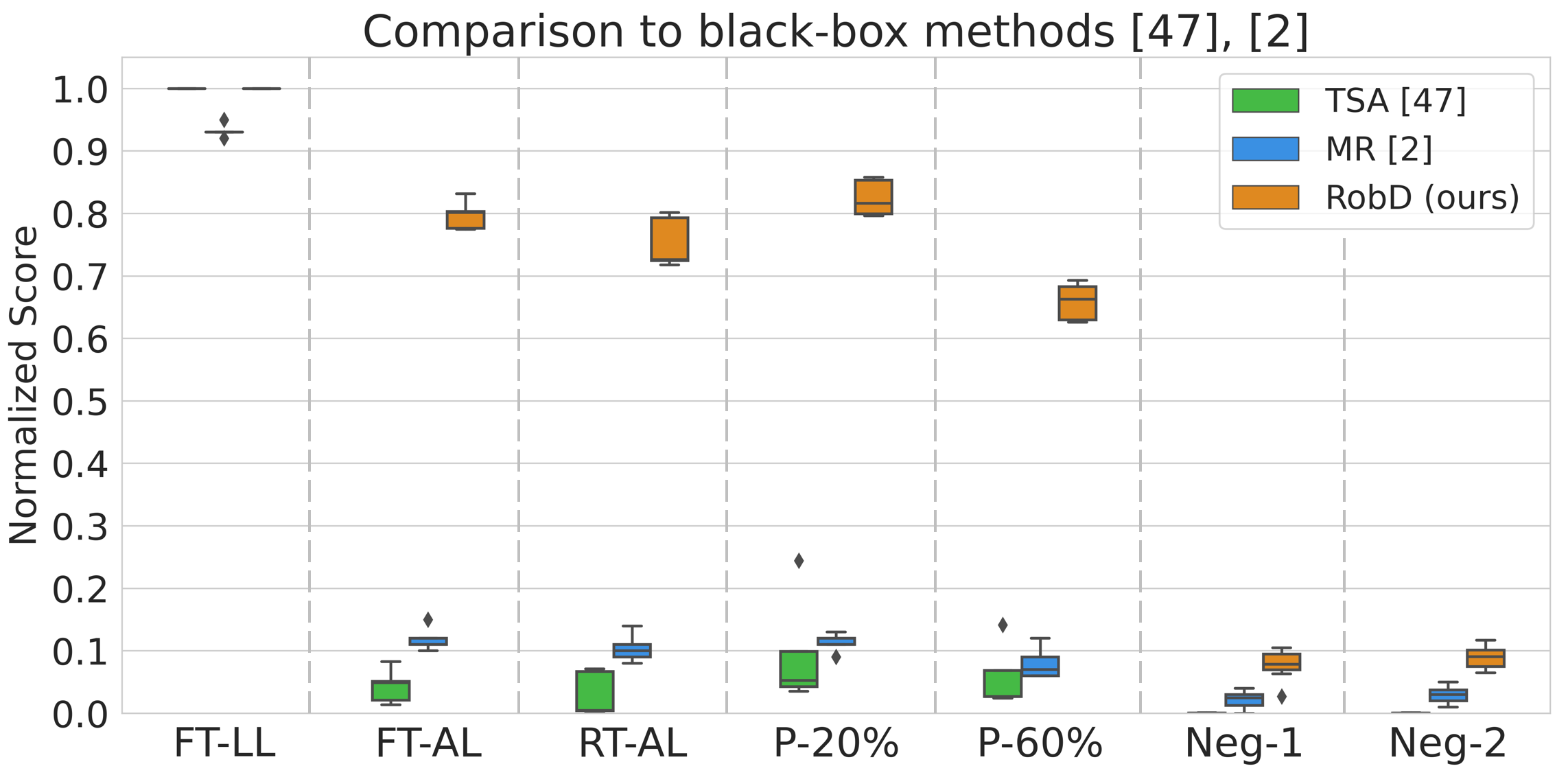
Black-box: Comparison to Watermarking and Fingerprinting. DNNWatermarking [47] is a black-box watermarking method based on backdoors, and IPGuard [2] is a black-box fingerprinting method based on targeted adversarial attacks. Here, we compare these two baselines with DeepJudge in the black-box setting. For DNNWatermarking, we train the watermarked model (i.e., victim model) using additionally patched samples from scratch to embed the watermarks, and the TSA (Trigger Set Accuracy) of the suspect model is calculated for ownership verification. IPGuard first generates targeted adversarial examples for the watermarked model then calculates the MR (Matching Rate) (between the victim and the suspect) for verification. For DeepJudge, we only apply the RobD (robustness distance) metric here for a fair comparison.

The left subfigure of Fig. 6 visualizes the results. DeepJudge demonstrates the best overall performance in this black-box setting. DNNWatermarking and IPGuard fail to identify the positive suspect models duplicated by FT-AL, RT-AL, P-20% and P-60%. Their scores (TSA and MR) drop drastically against these four attacks. This basically means that the embedded watermarks are completely removed, or the fingerprint can no longer be verified. While for the RobD metric of DeepJudge, the gap remains huge between the negative and positive suspects, demonstrating much better effectiveness to diverse finetuning and pruning attacks.

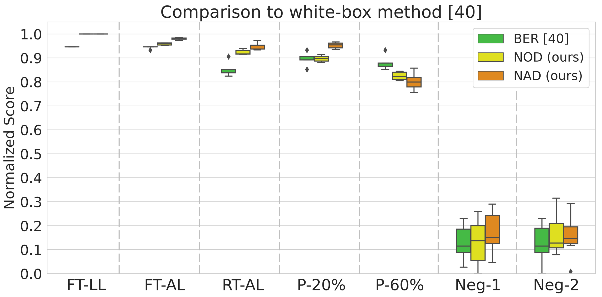
White-box: Comparison to Watermarking. EmbeddingWatermark [40] is a white-box watermarking method based on signatures. It requires access to model parameters for signature extraction. We train the victim model with the embedding regularizer [40] from scratch to embed a 128-bits signature. The BER (Bit Error Rate) is calculated and used to measure the verification performance. The right subfigure of Fig. 6 visualizes the comparison results to two white-box DeepJudge metrics NOD and NAD. The three metrics demonstrate a comparable performance with NAD wins on 4 out of the 5 positive suspects. Note that the huge gap between the positives and negatives indicates that all metrics can correctly identify the positive suspects. Here, a single metric of DeepJudge was able to achieve the same level of protection as EmbeddingWatermark.

TABLE VI: Performance of DeepJudge against model extraction attacks in the black-box setting. PGD [28] is used to generate adversarial test cases. ACC is the validation accuracy. For each metric, the values below (indicating ‘copy’) or above (indicating ‘not copy’) the threshold $\tau_{\lambda}$ (the last row) are highlighted in red (copy alert) and green (no alert), respectively. ‘Yes (2/2)’: two of the metrics vote for positive ($p_{copy}=100\%$); ‘No (0/2)’: none of the metrics vote for positive ($p_{copy}=0\%$). See more details about the 3 extraction attacks in Appendix A-F.

Model Type

MNIST

CIFAR-10

SpeechCommands

ACC

RobD

JSD

Copy?

ACC

RobD

JSD

Copy?

ACC

RobD

JSD

Copy?

Positive Suspect Models

JBA

83.6$\pm$1.7%

0.866$\pm$0.034

0.596$\pm$0.006

No (0/2)

40.3$\pm$1.5%

0.497$\pm$0.044

0.541$\pm$0.015

No (1/2)

40.1$\pm$1.7%

0.381$\pm$0.030

0.470$\pm$0.011

No (1/2)

Knock

94.8$\pm$0.6%

0.491$\pm$0.032

0.273$\pm$0.021

Yes (2/2)

74.4$\pm$1.0%

0.715$\pm$0.018

0.436$\pm$0.019

Yes (2/2)

86.6$\pm$0.5%

0.618$\pm$0.012

0.303$\pm$0.007

Yes (2/2)

ESA

88.7$\pm$2.5%

0.175$\pm$0.056

0.141$\pm$0.042

Yes (2/2)

67.1$\pm$1.9%

0.144$\pm$0.031

0.249$\pm$0.033

Yes (2/2)

$\times$

$\times$

$\times$

–

Negative Suspect Models

Neg-1

98.4$\pm$0.3%

0.968$\pm$0.014

0.614$\pm$0.016

No (0/2)

84.2$\pm$0.6%

0.920$\pm$0.021

0.603$\pm$0.016

No (0/2)

94.9$\pm$0.7%

0.817$\pm$0.025

0.456$\pm$0.014

No (0/2)

Neg-2

98.3$\pm$0.2%

0.949$\pm$0.029

0.600$\pm$0.020

No (0/2)

84.9$\pm$0.5%

0.926$\pm$0.030

0.615$\pm$0.021

No (0/2)

94.5$\pm$0.8%

0.832$\pm$0.024

0.472$\pm$0.012

No (0/2)

$\tau_{\lambda}$

–

0.852

0.538

–

–

0.816

0.537

–

–

0.727

0.405

–

V-C Defending Against Model Extraction

Model extraction (also known as model stealing) is considered to be a more challenging threat to DNN copyright. In this part, we evaluate DeepJudge against model extraction attacks, which has not been thoroughly studied in prior work.

V-C1 Attack strategies

We consider model extraction with two different types of supporting data: auxiliary or synthetic (see Section III). We consider the following state-of-the-art model extraction attacks: a) JBA (Jacobian-Based Augmentation [33]) samples a set of seeds from the test dataset, then applies Jacobian-based data augmentation to synthesize more data from the seeds. b) Knockoff (Knockoff Nets [32]) works with an auxiliary dataset that shares similar attributes as the original training data used to train the victim model. c) ESA (ES Attack [45]) requires no additional data but a huge amount of queries. ESA utilizes an adaptive gradient-based optimization algorithm to synthesize data from random noise. ESA could be applied in scenarios where it is hard to access the task domain data, such as personal health data. With the extracted data, the adversary can train a new model from scratch, assuming knowledge of the victim model’s architecture. The new model is considered as a successful stealing if its performance matches with the victim model.

V-C2 Failure of watermarking

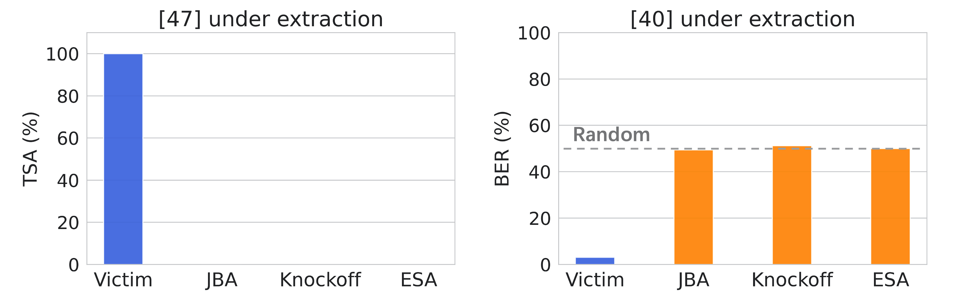
Our experiments in Section V-B show the effectiveness and robustness of watermarking to finetuning and pruning attacks. Unfortunately, here we show that the embedded watermarks can be removed by model extraction attacks. We show the results of DNNWatermarking and EmbeddingWatermark in Fig. 12. The extracted models by different extraction attacks all differ greatly from the victim model according to either TSA (from DNNWatermarking) or BER (from EmbeddingWatermark). For example, the TSA value for the victim model is 100%, however, the TSA values for the three extracted copies are all below 1%. This basically means that the original watermarks are all erased in the extracted models. It will inevitably lead to failed ownership claims. This is somewhat not too surprising as watermarks are task-irrelevant contents and not the focus of model extraction.

V-C3 Effectiveness of DeepJudge

Table VI summarizes the results of DeepJudge, which successfully identifies all positive suspect models, except when the stolen copies (by JBA) have extremely poor performance with 15%, 44% and 55% lower accuracy than the corresponding victim model. We note that model extraction does not always work, and poorly performed extractions are less likely to pose a real threat. We also observe that DeepJudge works better when the extraction is better, which therefore counters the ultimate perfect matching goal of model extraction attacks.

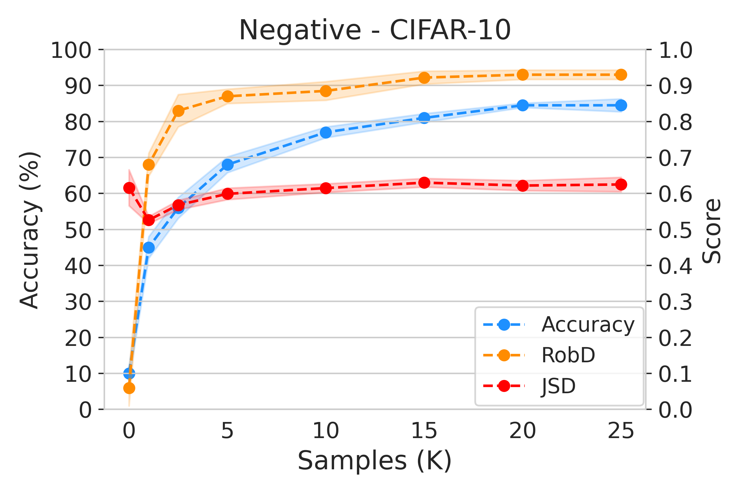
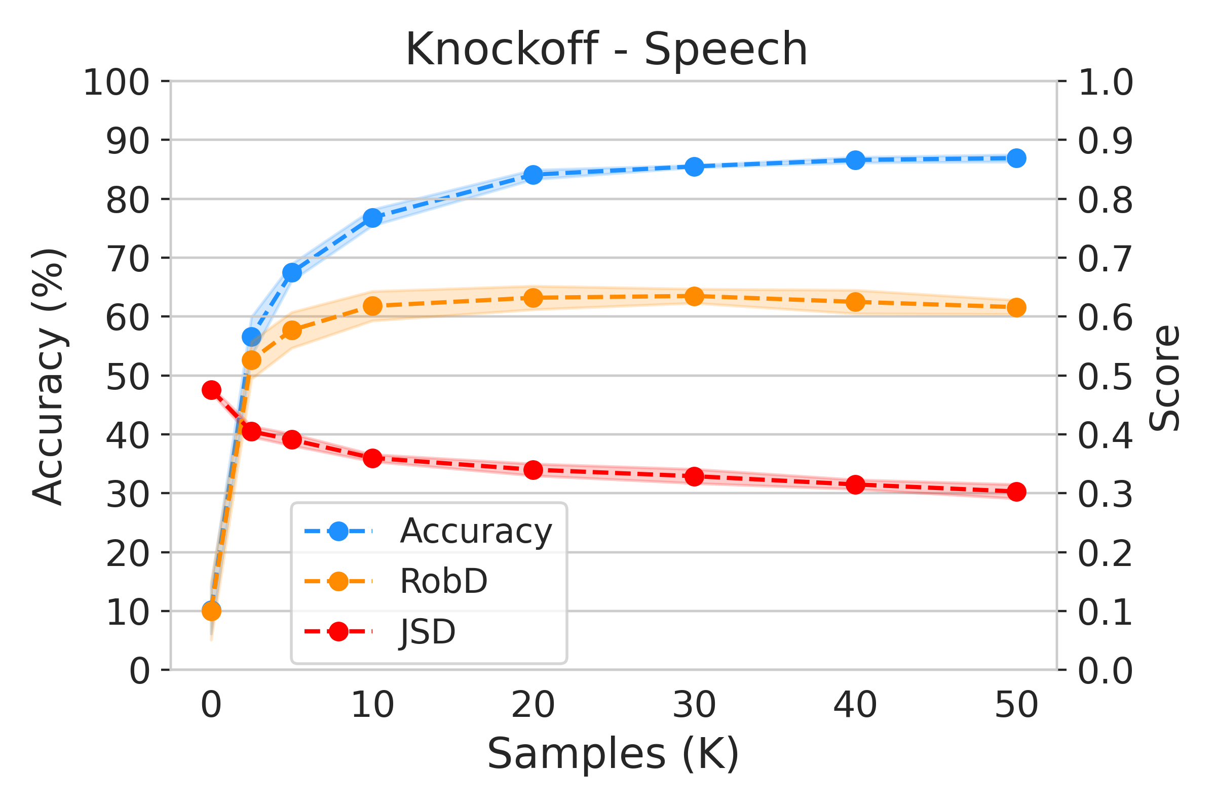
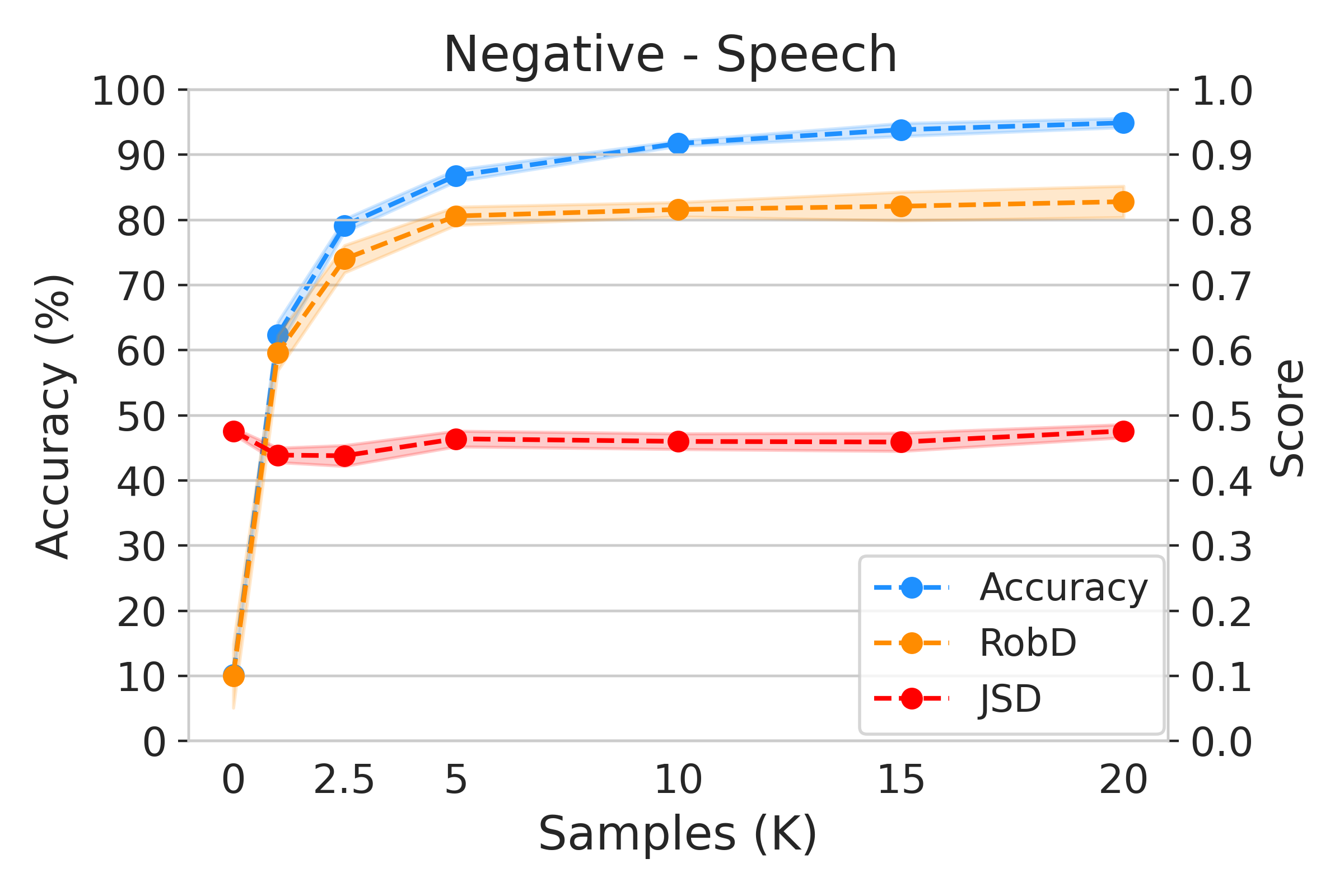
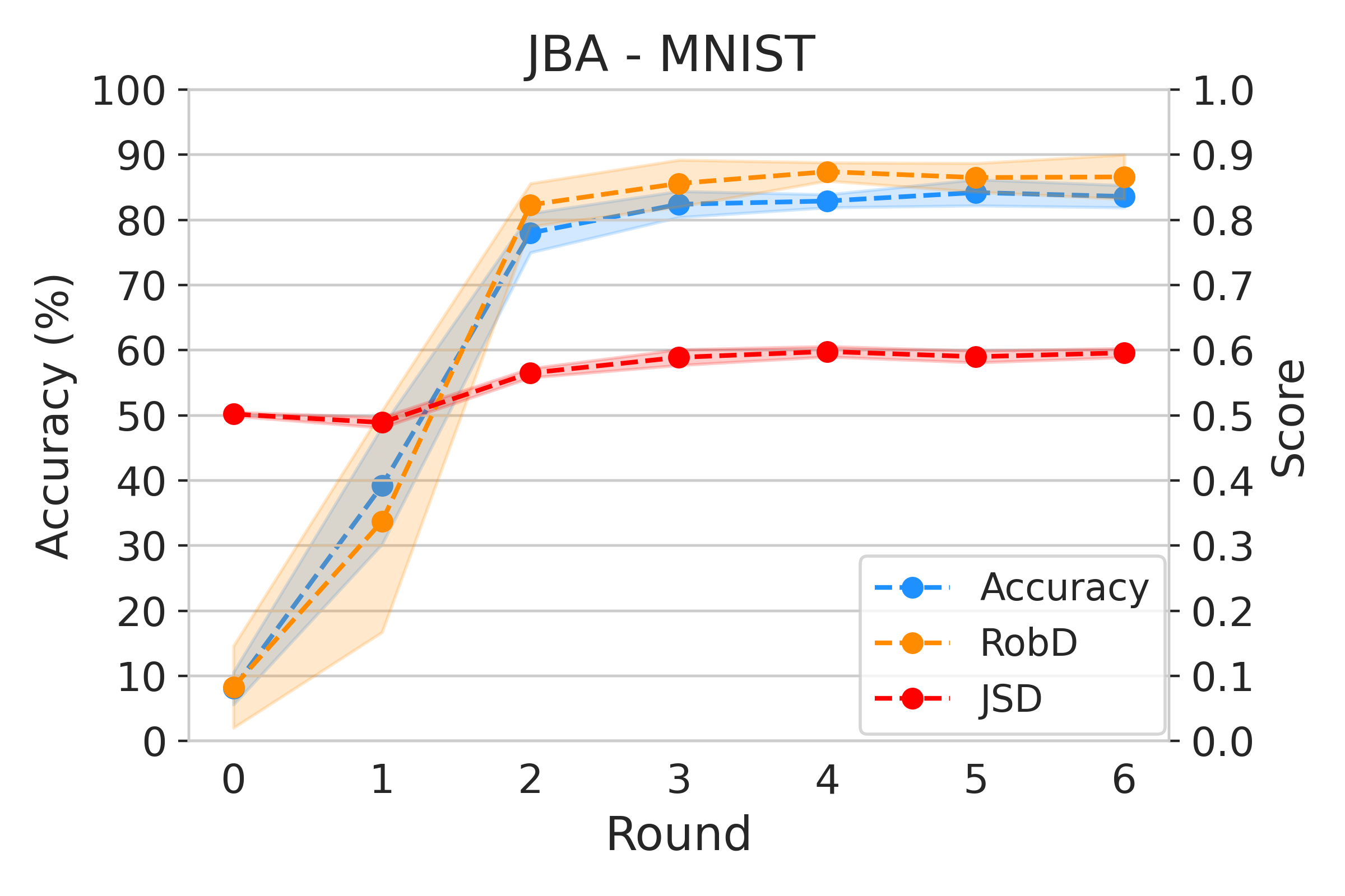
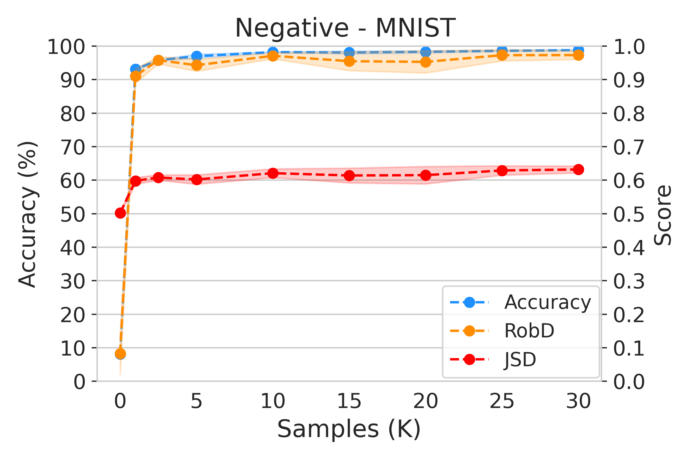
Compared to model finetuning or pruning, the average RobD and JSD values on extracted models are relatively larger, meaning that the decision boundaries of extracted models are more different from that of the victim model. The reason is that extracted models are often trained from a random point, while finetuning only slightly shifts the original boundary of the victim model, as depicted in Fig. 2. As such, model extraction is more stealthy and more challenging for ownership verification. Nonetheless, the two metrics RobD and JSD, can still reveal the unique similarities (smaller values) of the extracted models to the victim model: the better the extraction (higher accuracy of the extracted model), the lower the RobD and JSD values. This indicates that the extracted model behaves more similarly to the victim as its decision boundary gradually approaching that of the victim, and also highlights the unique advantage of DeepJudge against model extraction attacks. Note that JBA attack can only extract 50% of the original accuracy on either CIFAR-10 or SpeechCommands, which should not be considered as successful extractions.

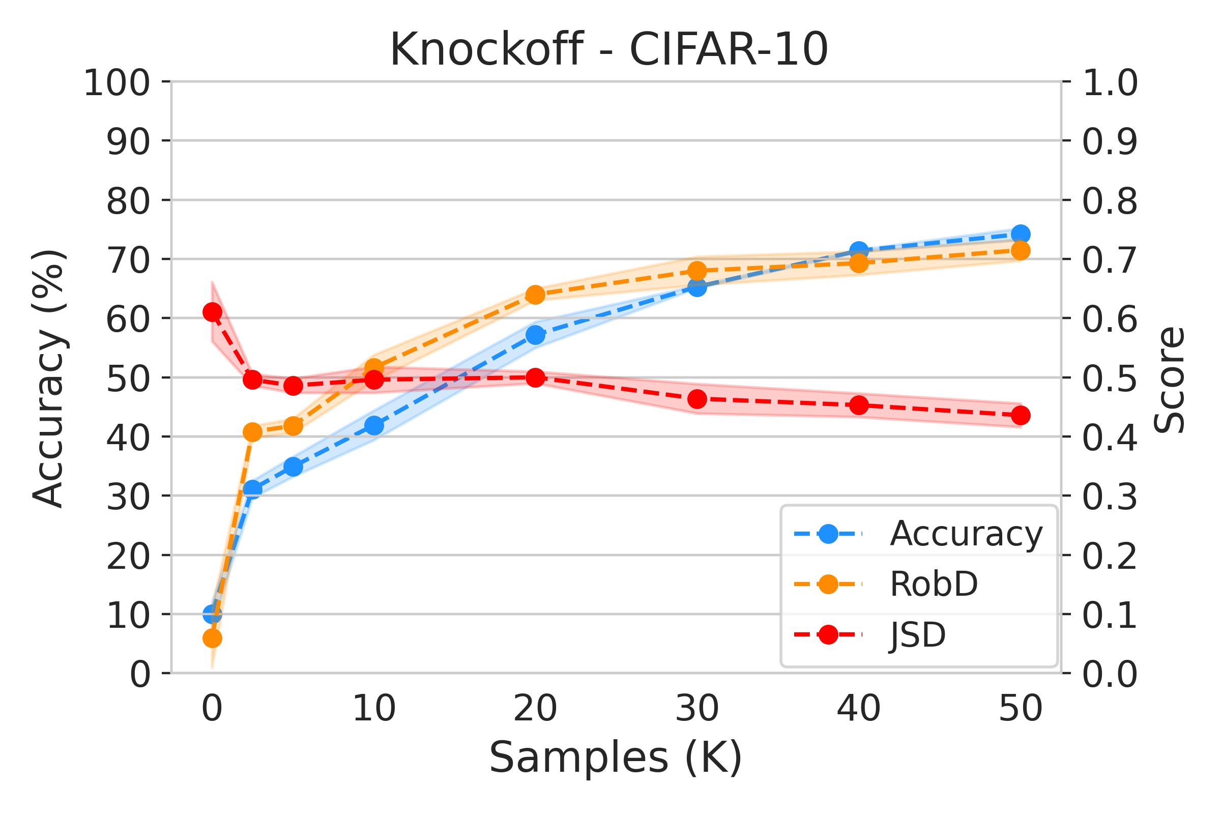
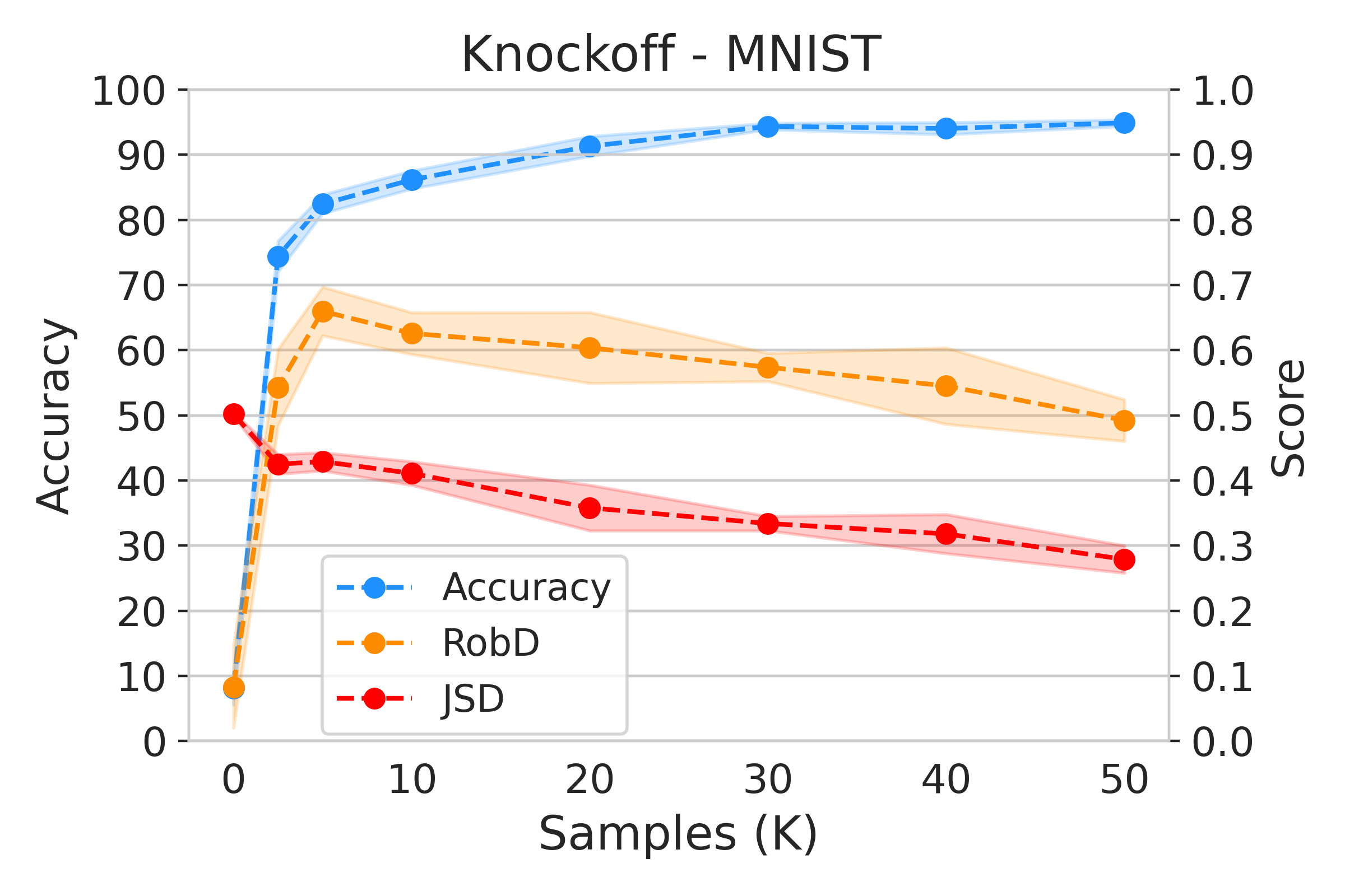
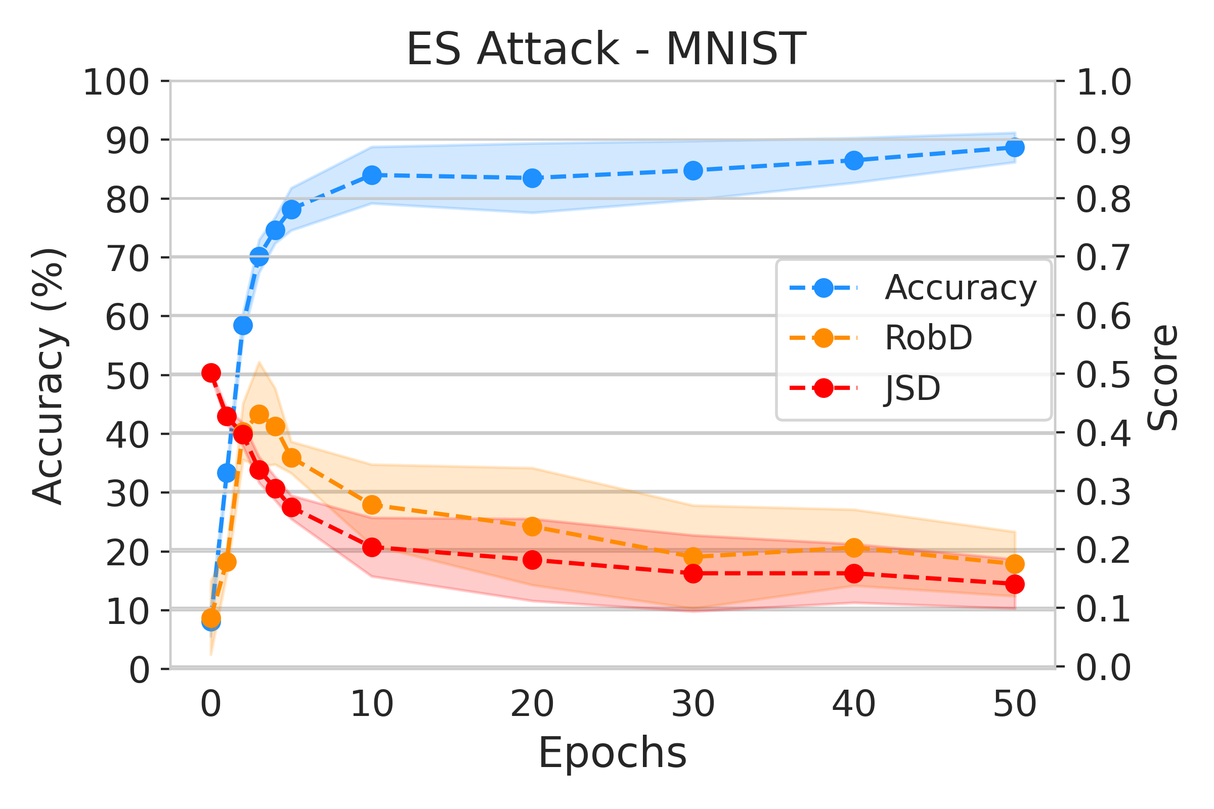
In Fig. 7, we further show the evolution of the RobD and JSD values throughout the entire extraction process of Knockoff, ESA and JBA attacks. We find that both RobD (orange line) and JSD (red line) values decrease as the extraction progresses, again, except for JBA. This confirms our speculation that, when tested by DeepJudge, a better extracted model will expose more similarities to its victim. By contrast, we also study how these two values change during the training process of the negative model in Fig. 7, which shows that the independently trained negative suspect models tend to vary more from the victim model and produce higher RobD and JSD values.

Figure 7: The RobD (orange line) and JSD (red line) scores between the victim and extracted models throughout the entire extraction procedure (defined by sample sizes, epochs or rounds) on MNIST.

VI Robustness to Adaptive Attackers

In this section, we explore potential adaptive attacks to DeepJudge based on the adversary’s knowledge of DeepJudge: 1) the adversary knows the testing metrics and the test cases, or 2) the adversary only knows the testing metrics. Contrast evaluation of watermarking & fingerprinting against similar adaptive attacks are in Appendix A-G.

VI-A Knowing Both Testing Metrics and Test Cases

In this threat model, the adversary has full knowledge of DeepJudge including the testing metrics $\Lambda$ and the secret test cases $T$. We also assume the adversary has a subset of clean data. In DeepJudge, we have two test settings, i.e., white-box testing and black-box testing. The two testings differ in the testing metrics and the generated test cases (see examples in Fig. 17). The black-box test cases are labeled. Therefore, the adversary can mix $T$ into its clean subset to finetune the stolen model to have large testing distances (i.e., black-box testing metrics RobD and JSD) while maintaining good classification performance. This will fool DeepJudge to identify the stolen model to be significantly different from the victim model. This adaptive attack against black-box testing is denoted by Adapt-B. Since the white-box test cases are unlabeled, the adversary can use the predicted labels (by the victim model) as ground-truth and finetunes the stolen model following a similar procedure as Adapt-B. This attack against white-box testing is denoted by Adapt-W. Note that the suffix ‘-B/-W’ marks the target testing setting to attack, while both attacks are white-box adaptive attacks knowing all the information.

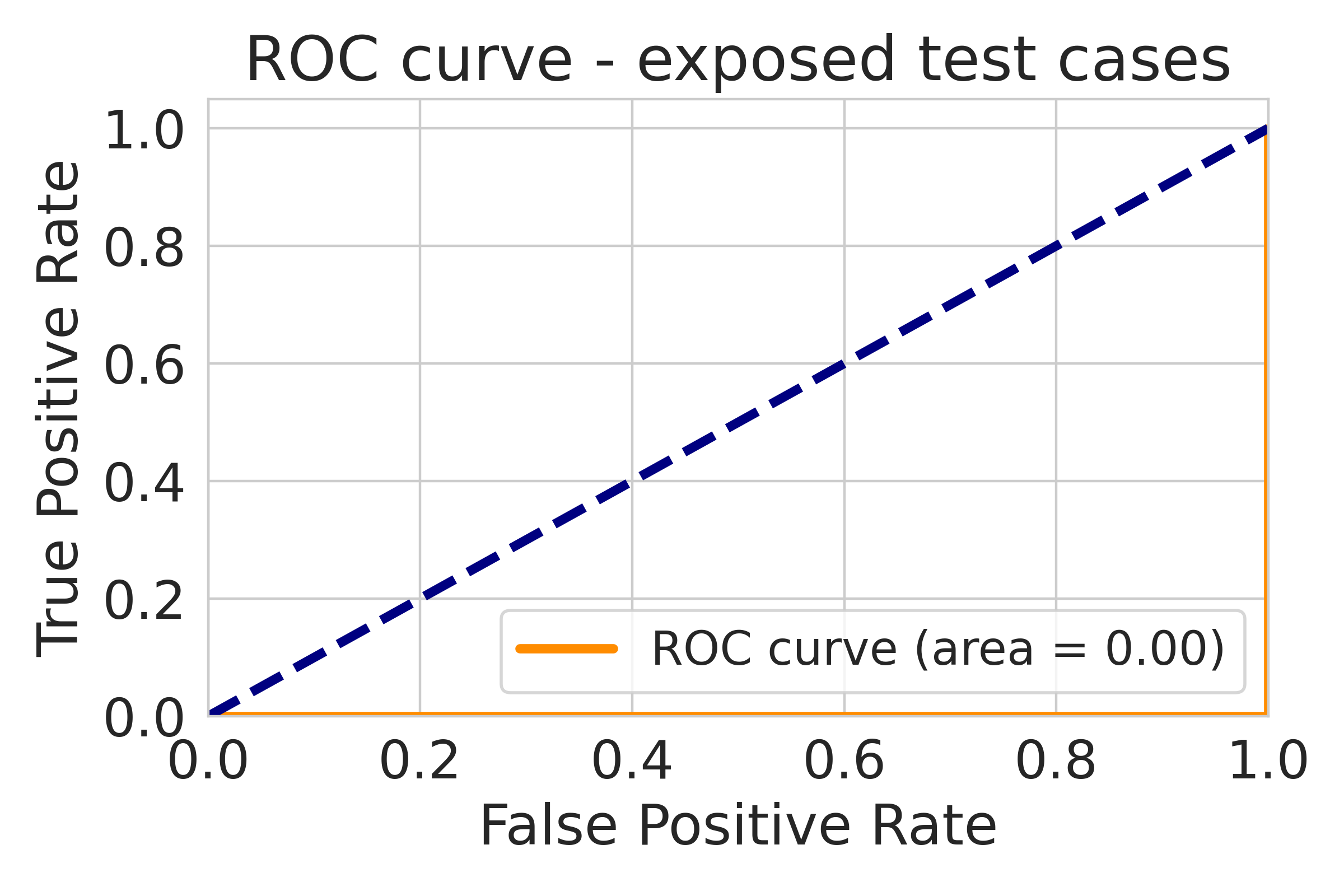
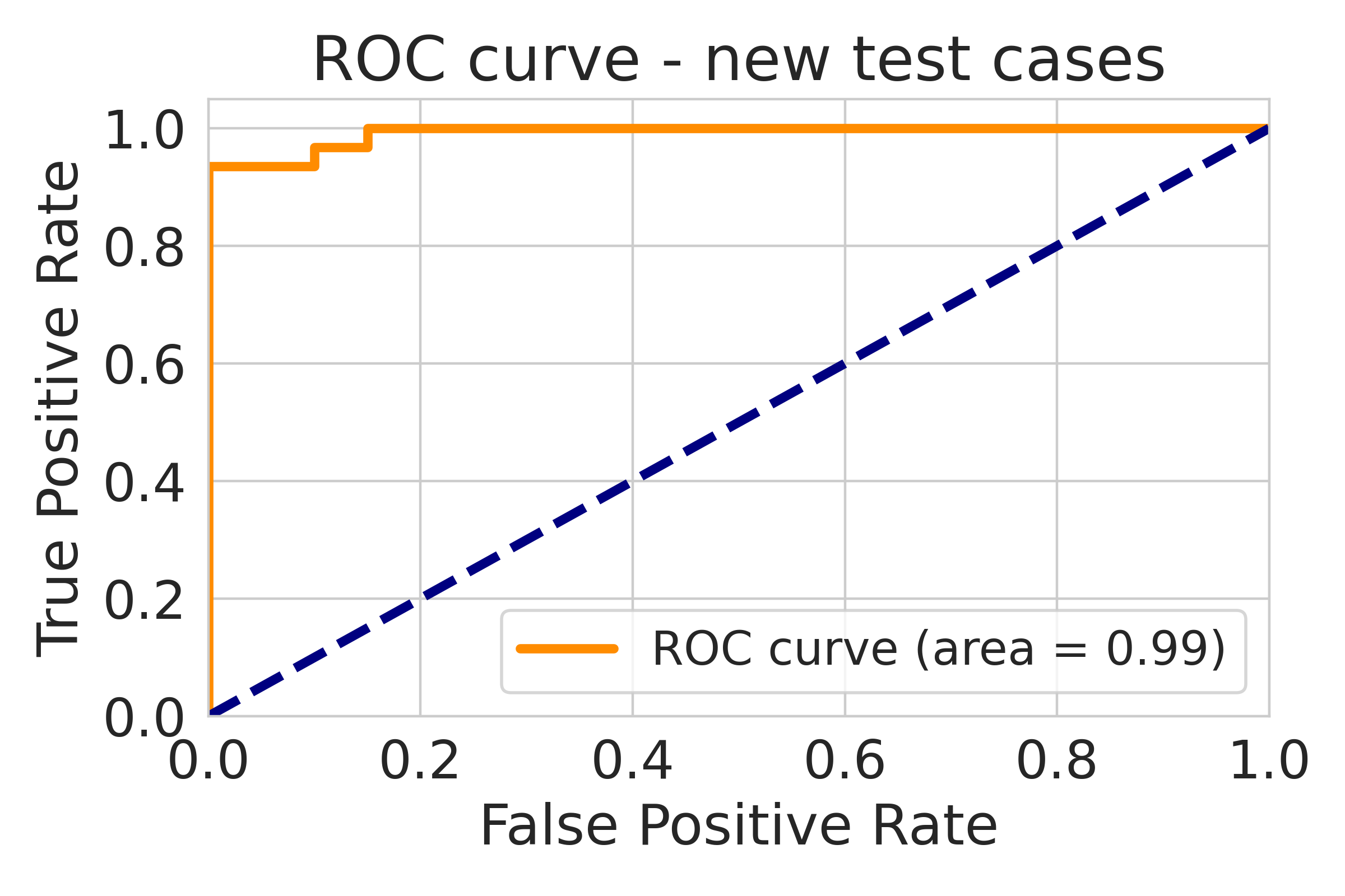
The results of DeepJudge using the exposed test cases $T$ are reported in Table VII. It shows that: 1) DeepJudge is robust to Adapt-W, which fails to maximize the output distance and activation distance simultaneously nor maintaining the original classification accuracy; 2) though DeepJudge is not robust to Adapt-B when the test cases are exposed with labels, it can easily recover the performance with new test cases generated with different seeds (see the ROC curves on the exposed and new test cases in Fig. 8); and 3) DeepJudge can still correctly identify the stolen copies by Adapt-B when combining black-box and white-box testings (the final judgements are all correct). Comparing the non-trivial effort of retraining/finetuning a model to the efficient generation of new test cases, DeepJudge holds a clear advantage in the arms race against finetuning-based adaptive attacks.

It is noteworthy that Adapt-W did not break all white-box metrics of DeepJudge, since the mechanism of white-box testing is robust. Specifically, black-box testing characterizes the behaviors of the output layer, while white-box testing characterizes the internal behaviors of more shallow layers. Due to the over-parameterization property of DNNs, it is relatively easy to fine-tune the model to overfit the set of black-box test cases, subverting the results of the black-box metrics. However, in white-box testing, changing the activation status of all hidden neurons on the set of white-box test cases is almost impossible without completely retraining the model. Therefore, white-box testing is inherently more robust to adaptive attacks, especially when the test cases are exposed.

Figure 8: Detection ROC curve of RobD with exposed (left) and new (right) test cases against Adapt-B attack on CIFAR-10.

VI-B Knowing Only the Testing Metrics

In this threat model, the adversary can still adapt in different ways. We consider two adaptive attacks: adversarial training targeting on black-box testing and a general transfer learning attack on white-box testing, respectively.

VI-B1 Blind adversarial training

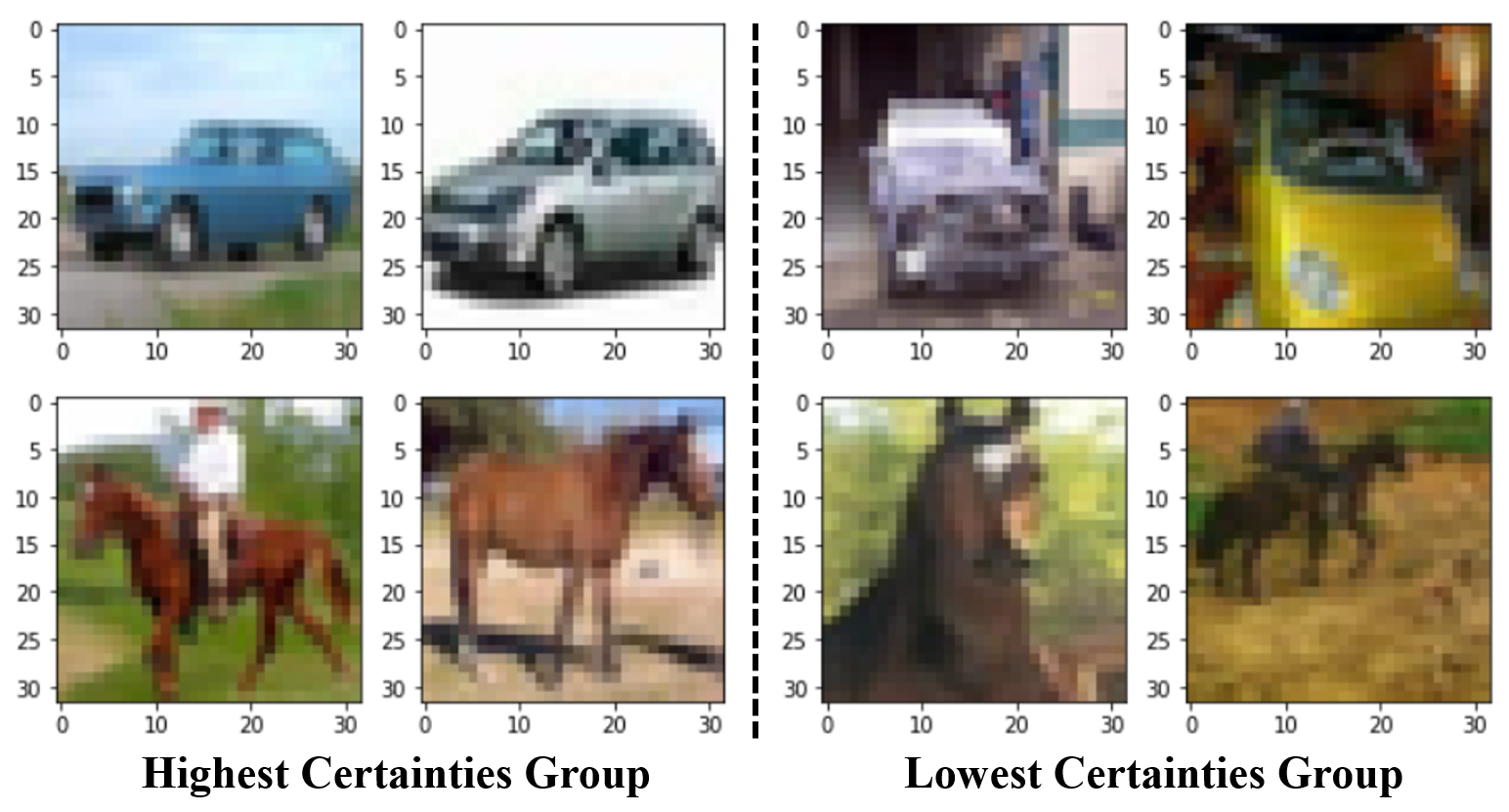
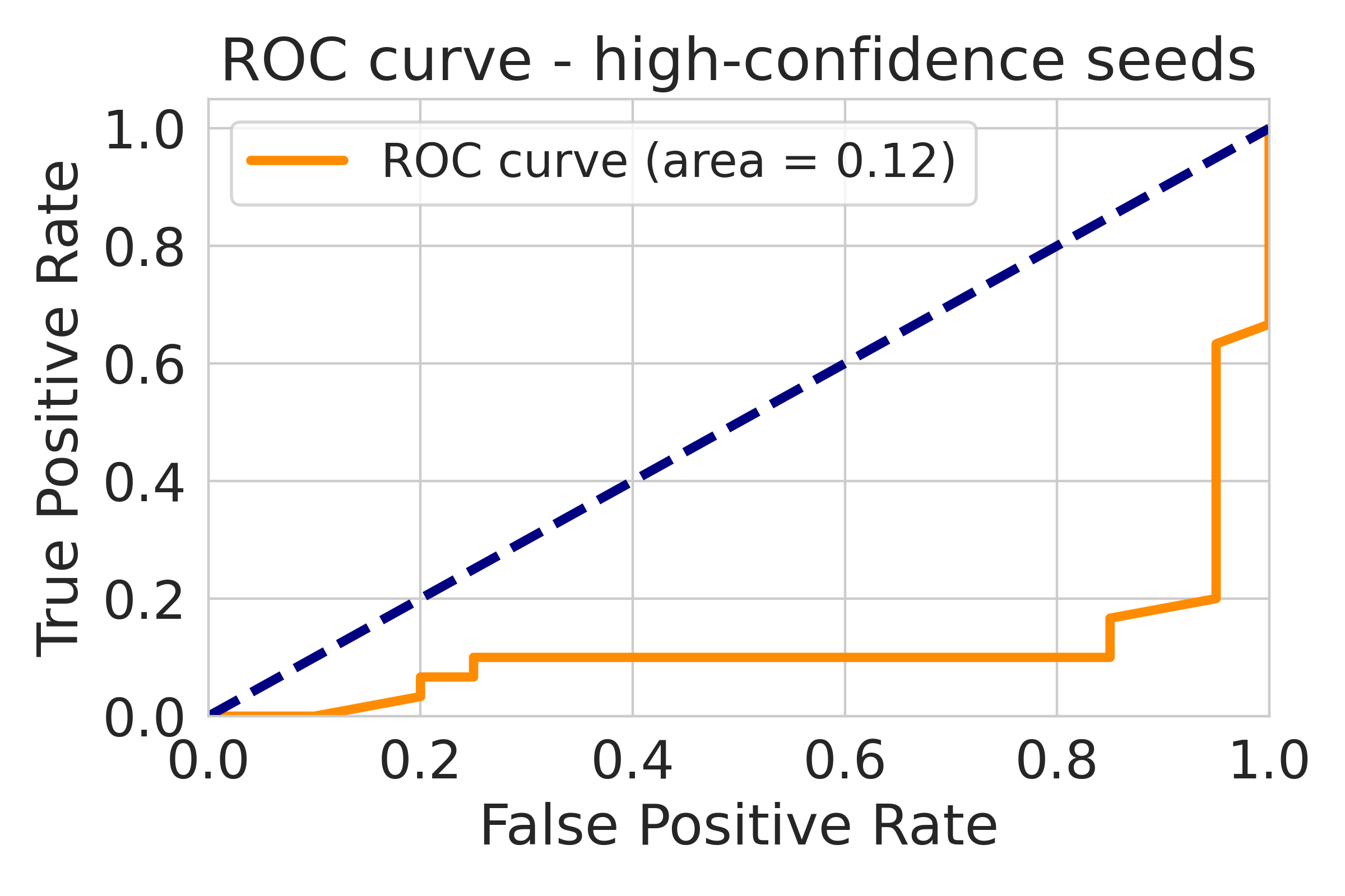
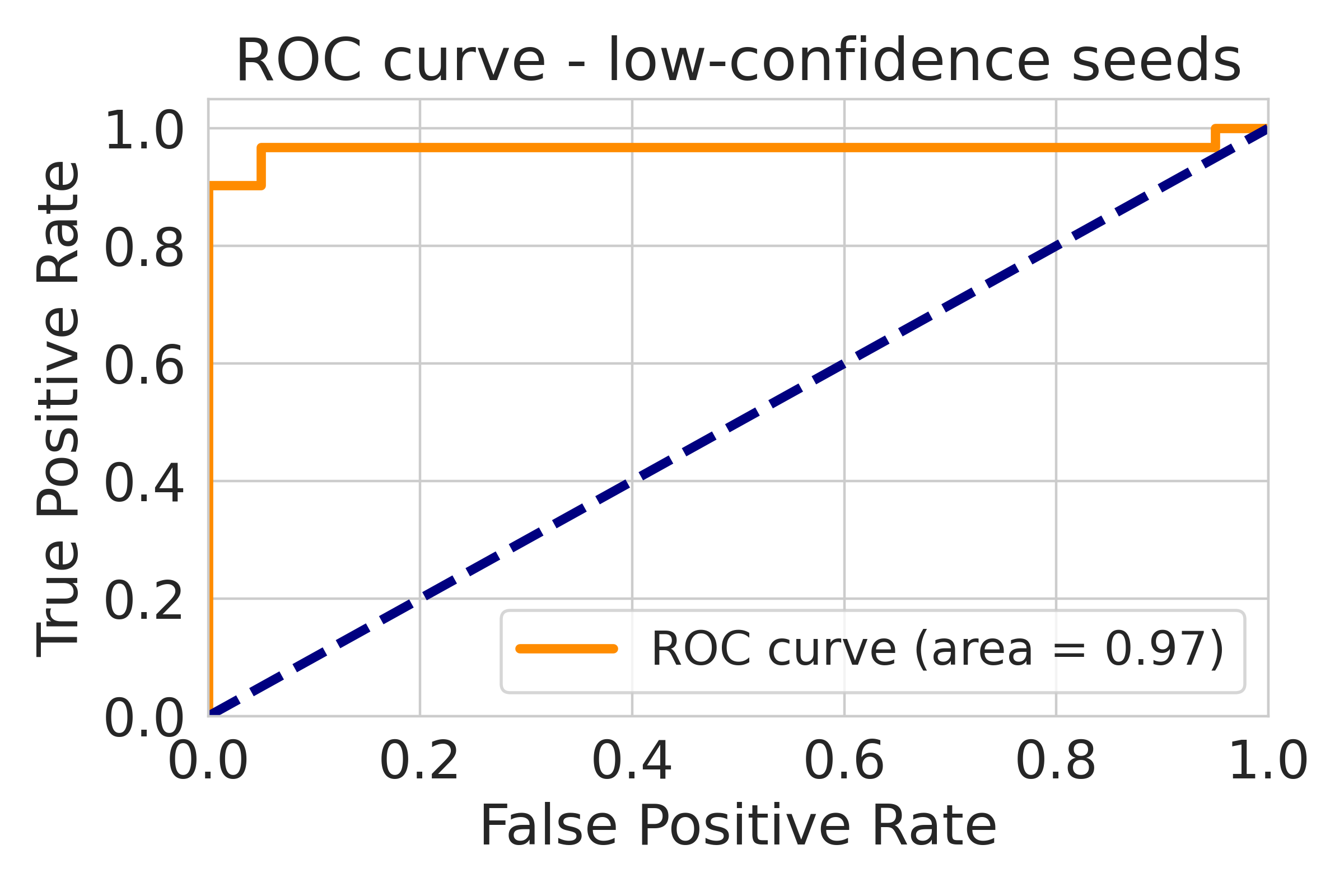
Since our black-box testing mainly relies on probing the decision boundary difference using adversarial test cases, the adversary may utilize adversarial training to improve the robustness of the stolen copy. Given the PGD parameters and a subset of clean data (20% of the original training data), the adversary iteratively trains the stolen model to smooth the model decision boundaries following [28]. This type of adaptive attack is denoted by Adv-Train. As Table VII shows, it can indeed circumvent our black-box testing, with a sacrifice of $\sim 10\%$ performance (a phenomenon known as accuracy-robustness trade-off [39, 46]). However, interestingly, if we replace the high-confidence seeds used in DeepJudge with low-confidence seeds, DeepJudge becomes effective again (as shown in Fig. 9). One possible reason is that, compared to high-confidence seeds, these low-confidence seeds are natural boundary (hard) examples that are close to the decision boundary, thus can generate more test cases to cross the adversarially smoothed decision boundary within certain perturbation budget. Examples of high/low confidence test seeds are provided in Fig. 15. It is also worth mentioning that our white-box testing still performs well in this case. Overall, DeepJudge is robust to Adv-Train or at least can be made robust by efficiently updating the seeds.

TABLE VII: Performance of DeepJudge against several adaptive attacks on the CIFAR-10 dataset. Adapt-B: adaptive attack against black-box testing; Adapt-W: adaptive attack against white-box testing; Adv-Train: adversarial training, VTL: vanilla transfer learning. For each metric, the values below (indicating ‘copy’) or above (indicating ‘not copy’) the threshold $\tau_{\lambda}$ (the last row) are highlighted in red (copy alert) and green (no alert) respectively.

Model Type			Black-box Testing		White-box Testing
		ACC	RobD	JSD	NOD	NAD	LOD	LAD	Copy?
Positive Suspect Models	Adapt-B	81.4$\pm$0.9%	0.985$\pm$0.011	0.665$\pm$0.007	0.38$\pm$0.04	0.44$\pm$0.15	1.12$\pm$0.06	0.40$\pm$0.05	Yes (4/6)
	Adapt-W	71.9$\pm$1.8%	0.519$\pm$0.048	0.372$\pm$0.025	3.11$\pm$0.12	1.94$\pm$0.12	11.62$\pm$0.54	1.89$\pm$0.33	Yes (4/6)
	Adv-Train	74.5$\pm$2.3%	0.939$\pm$0.087	0.637$\pm$0.036	0.68$\pm$0.11	0.79$\pm$0.17	1.89$\pm$0.14	0.75$\pm$0.08	Yes (4/6)
	VTL	93.3$\pm$1.7%	$\times$	$\times$	0.85$\pm$0.23	1.08$\pm$0.14	2.58$\pm$0.24	0.64$\pm$0.15	Yes (4/4)
Negative Suspect Models	Neg-1	84.2$\pm$0.6%	0.920$\pm$0.021	0.603$\pm$0.016	3.09$\pm$0.30	10.94$\pm$1.74	11.85$\pm$1.01	5.41$\pm$0.67	No (0/6)
	Neg-2	84.9$\pm$0.5%	0.926$\pm$0.030	0.615$\pm$0.021	3.21$\pm$0.18	11.09$\pm$0.71	12.60$\pm$1.33	5.37$\pm$0.72	No (0/6)
	$\tau_{\lambda}$	–	0.816	0.537	1.79	6.14	6.89	3.01	–

Figure 9: Detection ROC curve of RobD with adversarial test cases generated from high-confidence (left) or low-confidence seeds (right) against Adv-Train attack on CIFAR-10.

VI-B2 Transfer learning

The adversary may transfer the stolen copy of the victim model to a new dataset. The adversary exploits the main structure of the victim model as a backbone and adds more layers to it. Here, we test a vanilla transfer learning (VTL) strategy from the 10-class CIFAR-10 to a 5-class SVHN [31]. The last layer of the CIFAR-10 victim model is first replaced by a new classification layer. We then fine-tune all layers on the subset of SVHN data. Note that, in this setting, the black-box metrics are no longer feasible since the suspect model has different output dimensions to the victim model, however, the white-box metrics can still be applied since the shallow layers are kept. The results are reported in Table VII. Remarkably, DeepJudge succeeds in identifying transfer learning attacks with distinctively low testing distances and an $AUC=1$.

In one recent work [29], it was observed that the knowledge of the victim model could be transferred to the stolen models. Dataset Inference (DI) technique was then proposed to probe whether the victim’s knowledge (i.e., private training data) is preserved in the suspect model. We believe such knowledge-level testing metrics could also be incorporated into DeepJudge to make it more comprehensive. An analysis of how different levels of transfer learning could affect DeepJudge can be found in Appendix A-H.

VII Conclusion

In this work, we proposed DeepJudge, a novel testing framework for copyright protection of deep learning models. The core of DeepJudge is a family of multi-level testing metrics that characterize different aspects of similarities between the victim model and a suspect model. Efficient and flexible test case generation methods are also developed in DeepJudge to help boost the discriminating power of the testing metrics. Compared to watermarking methods, DeepJudge does not need to tamper with the model training process. Compared to fingerprinting methods, it can defend more diverse attacks and is more resistant to adaptive attacks. DeepJudge is applicable in both black-box and white-box settings against model finetuning, pruning and extraction attacks. Extensive experiments on multiple benchmark datasets demonstrate the effectiveness and efficiency of DeepJudge. We have implemented DeepJudge as a self-contained open-source toolkit. As a generic testing framework, new testing metrics or test case generation methods can be effortlessly incorporated into DeepJudge to help defend future threats to deep learning copyright protection.

Appendix A Appendix

A-A Details of Datasets and Models

We use four benchmark datasets from two domains for the evaluation:

• MNIST [24]. This is a handwritten digits (from 0 to 9) dataset, consisting of 70,000 images with size $28\times 28\times 1$, of which 60,000 and 10,000 are training and test data.

• CIFAR-10 [22]. This is a 10-class image classification dataset, consisting of 60,000 images with size $32\times 32\times 3$, of which 50,000 and 10,000 are training and testing data.

• ImageNet [36]. This is a large-scale image dataset containing more than 1.2 million training images of 1,000 categories. It is more challenging due to the higher image resolution $224\times 224\times 3$. We randomly sample 100 classes to construct a subset of ImageNet, of which 120,000 are training data and 30,000 are testing data.

• Speech Commands [42]. This is an audio dataset of 10 single spoken words, consisting of about 40,000 training samples and 4,000 testing samples. We pre-processed the data to obtain a Mel Spectrogram [6]. Each audio sample is transformed into an array of size $120\times 85$.

To explore the scalability of DeepJudge, various model structures are tested as in Table III. LeNet-5, ResNet-20 and VGG-16 are standard CNN structures, while LSTM(128) is an RNN structure: an LSTM layer with 128 hidden units, followed by three fully-connected layers (128/64/10).

A-B Seed Selection Strategy

Seed selection is important for generating high-quality test cases. We use DeepGini [12] to measure the certainty of each candidate sample. Given the victim model $f$ and a testing dataset $\mathcal{D}$, we first calculate the Certainty Score (CS) for each seed ${\bm{x}}\in\mathcal{D}$ as: $CS(f^{L},{\bm{x}})=\sum_{i}^{C}f^{L}_{i}({\bm{x}})^{2},$ then we rank the seed list by the certainty score, and the first part of the seeds of the highest scores (i.e., most certainties) will be chosen for the following generation process. Here, we assume to have two seeds $\{{\bm{x}}_{1},{\bm{x}}_{2}\}$ with $CS(f^{L},{\bm{x}}_{1})>CS(f^{L},{\bm{x}}_{2})$, that means the victim model $f$ is more confident at ${\bm{x}}_{1}$, which also means that ${\bm{x}}_{1}$ is farther from the decision boundary and easier for classification (see examples in Fig. 15).

A-C Data-augmentation

During the finetuning and pruning processes, typical data-augmentation techniques are used to strengthen the attacks except for the SpeechCommands dataset, including random rotation ($10^{\circ}$), random width- and height-shift (both $0.1$).

A-D Test Case Generation Details and Calibrations

Specifically, we consider three adversarial attacks for generating black-box test cases (see Section IV-C1).

FGSM [14] perturbs a normal example ${\bm{x}}$ by one single step of size $\epsilon$ to maximize the model’s prediction error with respect to the groundtruth label $y$:${\bm{x}}^{\prime}={\bm{x}}+\epsilon\cdot\operatorname{sign}(\bigtriangledown_{{\bm{x}}}\mathcal{L}(f^{L}({\bm{x}}),y))$, where $\operatorname{sign}(\cdot)$ is the sign function, $\mathcal{L}$ is the cross entropy (CE) loss, and $\bigtriangledown_{{\bm{x}}}\mathcal{L}$ is the gradient of the loss to the input.

PGD [28] is an iterative version of FGSM but with smaller step size: ${\bm{x}}^{k}=\Pi_{\epsilon}({\bm{x}}^{k-1}+\alpha\cdot\operatorname{sign}(\bigtriangledown_{{\bm{x}}}\mathcal{L}(f^{L}({\bm{x}}^{k-1}),y)))$, where ${\bm{x}}^{k}$ is the adversarial example obtained at the $k$-th perturbation step, $\alpha$ is the step size and $\Pi_{\epsilon}$ is a projection (clipping) operation that projects the perturbation back onto the $\epsilon$-ball centered around ${\bm{x}}$ if it goes beyond.

CW [4] generates adversarial examples by solving the optimization problem: ${\bm{x}}^{\prime}=\underset{{\bm{x}}^{\prime}}{\min}\left\lVert{\bm{x}}^{\prime}-{\bm{x}}\right\rVert_{2}^{2}-c\cdot\mathcal{L}(f^{L}({\bm{x}}^{\prime}),y)$, where $c$ is a hyperparameter balancing the two terms and the pixel values of adversarial example ${\bm{x}}^{\prime}$ are bounded to be within a legitimate range, e.g., $[0,1]$ for 0-1 normalized input.

TABLE VIII: The hyper-parameters used in different test case generation strategies.

Method	Params	MNIST	CIFAR-10	ImageNet	SpeechCmds
PGD [28]	$\epsilon/steps$	0.1/10	0.03/10	0.01/10	0.1/10
Alg. 2	$m/iters$	3/1k	3/1k	3/1k	1/1k
FGSM [14]	$\epsilon/steps$	0.1/1	0.03/1	0.01/1	0.1/1
CW [4]	$c/iters$	5/1k	5/1k	5/1k	5/1k
IPG [2]	$k/iters$	10/1k	10/1k	10/1k	10/1k

TABLE IX: Time cost (seconds) of test cases generation.

Method	MNIST	CIFAR-10	ImageNet	SpeechCmds
PGD [28]	0.3	3.7	227.6	1.2
Alg. 2	635.3	1200.3	1280.1	4424.6

The hyper-parameters used for the generation algorithms on different datasets are summarized in Table VIII. Here, we take CIFAR-10 dataset as an example and analyze the influencing factors of the test case generation process.

Adversarial Examples. PGD is the default choice for generating adversarial examples in the black-box setting. Here, we further compare PGD with two other methods, FGSM and CW. We use the same selected seeds for the generation. Table X shows the results of the RobD metric. We observe that the gap in RobD values between the positive and negative suspect models is very small when CW is used, which fails to distinguish the two types of models. One reason is that CW attack optimizes adversarial examples for minimal perturbations, which is more sensitive (less robust) to model modifications. FGSM can be regarded as a one-step PGD, which usually has a larger average perturbation than PGD. When the perturbation increases, the RobD value of negative suspect models would decrease since adversarial examples with larger perturbations tend to have better transferability [43]. It is similar to PGD_3ϵ when the perturbation bound increases. In general, the absolute RobD gap between the positive and negative suspects tested with PGD-generated test cases is larger than that of FGSM and CW. Moreover, PGD is relatively cheaper to calculate than CW, i.e., the time cost of PGD is $100\times$ lower than CW. Overall, PGD is more suitable for fingerprinting the decision boundary with untargeted adversarial examples, as shown in Fig. 2. We will explore more effective metrics and test case generation methods with diverse granularity in future work.

TABLE X: Using different methods to generate adversarial examples for the RobD metric evaluation on CIFAR-10 dataset. PGD_ϵ/3 : with $\frac{1}{3}\times$ perturbation bound, PGD_3ϵ : with $3\times$ bound, PGD_10s: with $10\times$ steps.

Model Type		FGSM	CW	PGD	PGDϵ/3	PGD3ϵ	PGD10s
Positive Suspect Models	FT-LL	0.024$\pm$0.004	0.0$\pm$0.0	0.0$\pm$0.0	0.034$\pm$0.002	0.0$\pm$0.0	0$\pm$0.0
	FT-AL	0.261$\pm$0.025	0.905$\pm$0.028	0.192$\pm$0.028	0.733$\pm$0.012	0.046$\pm$0.010	0.350$\pm$0.027
	RT-AL	0.267$\pm$0.025	0.917$\pm$0.024	0.237$\pm$0.055	0.748$\pm$0.046	0.073$\pm$0.022	0.400$\pm$0.046
	P-20%	0.252$\pm$0.030	0.882$\pm$0.038	0.155$\pm$0.032	0.702$\pm$0.023	0.045$\pm$0.020	0.299$\pm$0.049
	P-60%	0.293$\pm$0.027	0.940$\pm$0.013	0.318$\pm$0.036	0.792$\pm$0.023	0.123$\pm$0.022	0.502$\pm$0.031
Negative Suspect Models	Neg-1	0.662$\pm$0.058	0.999$\pm$0.002	0.920$\pm$0.021	0.989$\pm$0.007	0.573$\pm$0.093	0.958$\pm$0.013
	Neg-2	0.672$\pm$0.019	0.998$\pm$0.003	0.926$\pm$0.030	0.986$\pm$0.004	0.576$\pm$0.030	0.948$\pm$0.012
	$\tau_{\lambda}$	0.583	0.897	0.816	0.886	0.489	0.851

Layer Selection. Layer selection is important when applying DeepJudge in the white-box setting with NOD and NAD. Here, we evaluate how the choice of layers affects the performance of DeepJudge. For comparison, we choose a shallow layer and a deep layer of the victim model, and re-generate the test cases respectively for each layer. Fig. 10 shows the results of NOD and NAD metrics. In general, the NOD/NAD difference between the positive and negative suspect models becomes much larger at the shallow layer. The reason is that the shallow layers of a network usually learn the low-level features [44], and they tend to stay the same or at least similar during model finetuning. Particularly, the performance on RT-AL degrades the most when the deep layer is selected, since the parameters of the last layer are re-initialized. Thus, choosing the shallow layers to compute the NOD and NAD metrics could help the robustness of DeepJudge. Moreover, the time cost of generating and testing with the shallow layer is 10$\times$ less than the deep layer, since most of the back-propagation computations are eliminated.

Figure 10: Normalized distance evaluations based on different layers of the CIFAR-10 network: ‘-Shallow’ means the results on the shallow layer, and ‘-Deep’ means the deep layer.

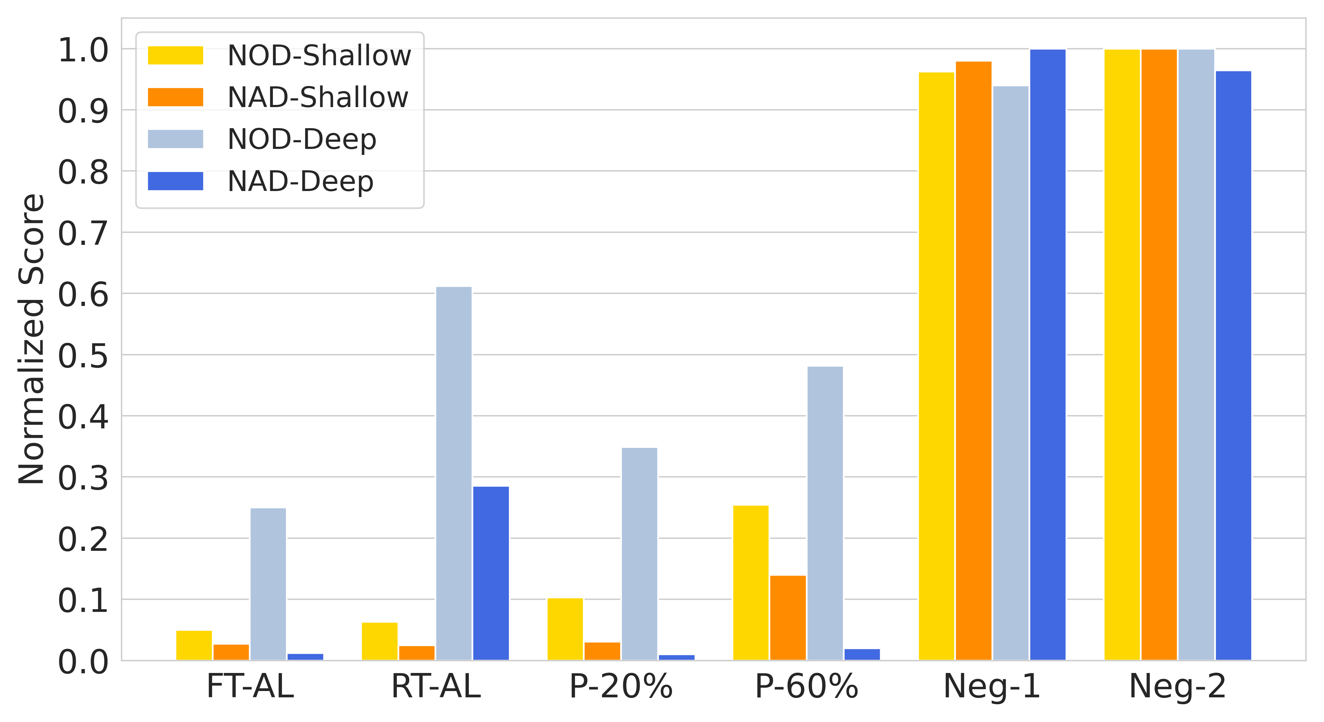
A-E Defense Baselines

A-E1 Backdoor-based watermarking (Black-box)

[47] embeds backdoors into the model. In our experiments, we select 500 samples from the training dataset, of which the ground truth labels are “automobile”. Then we patch an “apple” logo at the bottom right corner of each sample and change their labels to “cat” (see Fig. 11). These trigger examples (i.e., trigger set) are mixed into the clean training dataset to train a watermarked model from scratch. The initial TSA of the watermarked model is 100.0% (on a separate trigger set).

Figure 11: A trigger input example used in backdooring.

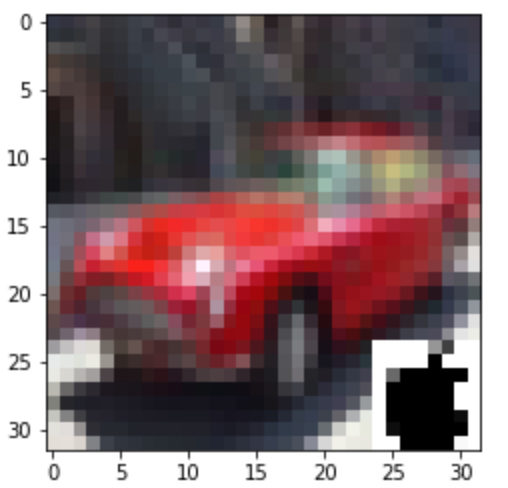
A-E2 Signature-based watermarking (White-box)

[40] embeds a $T$-bit vector (i.e., the watermark) $b\in\{0,1\}^{T}$ into one of the convolutional layers, by adding an additional parameter regularizer into the loss function: $E(w)=E_{0}(w)+\lambda E_{R}(w),$ where $E_{0}(w)$ is the original task loss function, $E_{R}(w)$ is the regularizer that imposes a certain restriction on the model parameters $w$, and $\lambda$ is a hyper-parameter. In our experiments, $\lambda$ is set to $0.01$, and we embed a 128-bit watermark (generated by the random strategy) into the second convolutional block (Conv-2 group) as recommended in [40]. The initial BER of the watermarked model is 3.13%.

A-E3 Fingerprinting (Black-box)

IPGuard [2] proposes a type of adversarial attack that targets on generating adversarial examples $x^{\prime}$ around the classification boundaries of the victim model, and the matching rate (MR) of these key samples is calculated for the verification similar to [47]. We generate a set of 1,000 adversarial examples following [2] and the initial MR of the victim model on the generated key samples is 100.0%.

A-F Model Extraction Attacks

Jacobian-Based Augmentation. The seeds used for augmentation are all sampled from the testing dataset. We sample 150 seeds for extracting the MNIST victim model, 500 seeds for SpeechCommands, 1,000 seeds for CIFAR-10, and use all other default settings [33].

Knockoff Nets. We use the Fashion-MNIST dataset for extracting the MNIST victim model, an independent speech dataset for SpeechCommands, and CIFAR-100 for CIFAR-10. We use other default hyper-parameter settings of [32].

ES Attack. We use the OPT-SYN algorithm [45] to heuristically synthesize the surrogate data. We set the stealing epoch to 50 for MNIST and 400 for CIFAR-10. We failed to extract the SpeechCommands Victim model since the validation accuracy could not exceed 20%. All other hyper-parameters are the same as in [45].

^∗Functionality-equivalent Extraction. Besides the above three extraction attacks, we are also aware of the functionality-equivalent extraction attacks [19, 3] that attempt to obtain a precise functional approximation of the victim model. For instance, [3] proposed a differential attack that could steal the parameters of the victim model up to floating-point precision without the knowledge of training data. We remark that defending this type of attack is a trivial task for DeepJudge as there will be no difference between the extracted model and the victim model in an ideal approximation.

Note that Black-box model extraction is still underexplored, and more extraction attacks may appear in the future. This poses a continuous challenge for deep learning copyright protection. We hope that DeepJudge could evolve with the adversaries by incorporating more advanced testing metrics and test case generation methods, and provide a possibility to fight against this continuing model stealing threat.

A-G Adaptive Attacks for Watermarking & Fingerprinting

In addition to Section VI, here we conduct an extra evaluation of existing watermarking [40, 47] and fingerprinting [2] methods under similar adaptive attack settings.

Adaptive attacks. Adv-Train and VTL are the two adaptive attacks in Table VII, while the Adapt-X attack is specifically designed for each method as follows:

• Adapt-X for [40]. Since the embedded watermark (signature) is known, the adversary copies (steals) the victim model then fine-tunes it on a small subset of clean examples while maximizing the embedding loss $E_{R}(w)$ on the signature.

• Adapt-X for [47]. Since the embedded watermark (backdoor) is known, the adversary can follow a similar approach as above to steal the victim model and remove the backdoor watermark with a few backdoor-patched but correctly-labeled examples.

• Adapt-X for [2]. Similar to our Adapt-B for DeepJudge, the adversary copies the victim model then fine-tunes it on a small subset of clean and correctly-labeled fingerprint examples to circumvent fingerprinting.

As the results in Table XI show, all three methods are completely broken by the adaptive attacks. DeepJudge is the only method that can survive these attacks and was partially compromised but not fully broken (the final judgments are still correct, as shown in the ‘Copy?’ column of Table VII). This implies that a single metric of watermarking or fingerprinting is not sufficient enough to combat adaptive attacks. By contrast, a testing framework with comprehensive testing metrics and test case generation methods may have the required flexibility to address this challenge. For example, Adv-Train may break the black-box testing of DeepJudge but cannot break the white-box testing (see Section VI-B). Moreover, DeepJudge can quickly recover its performance by switching to a new set of seeds (see Fig. 9).

TABLE XI: Performance of existing watermarking and fingerprinting baselines on CIFAR-10 dataset against adaptive attacks: 1) Adapt-X, adaptive attack designed specifically against the defense method; 2) Adv-Train, blind adversarial training; and 3) VTL, vanilla transfer learning. The broken metrics (close to the negatives) are highlighted in red. Adapt-X breaks all three metrics, while Adv-Train breaks the adversarial-examples-based fingerprinting.

Model Type		Black-box Watermarking [47]		White-box Watermarking [40]		Black-box Fingerprinting [2]
		ACC	TSA	ACC	BER	ACC	MR
Victim Model		82.9%	100.0%	83.8%	3.13%	84.8%	100.0%
Positive suspect models	Adapt-X	81.8$\pm$0.8%	0.01$\pm$0.01%	71.2$\pm$2.6%	46.3$\pm$3.3%	81.9$\pm$0.2%	1.2$\pm$0.8%
	Adv-Train	73.8$\pm$1.6%	5.5$\pm$3.2%	73.5$\pm$1.7%	4.0$\pm$0.8%	74.5$\pm$2.3%	4.2$\pm$1.5%
	VTL	92.2$\pm$1.3%	$\times$	91.7$\pm$1.6%	6.1$\pm$1.2%	93.3$\pm$1.7%	$\times$
Negative models	Neg-1	84.2$\pm$0.6%	0.05$\pm$0.04%	84.2$\pm$0.6%	50.3$\pm$4.1%	84.2$\pm$0.6%	2.2$\pm$1.4%
	Neg-2	84.9$\pm$0.5%	0.03$\pm$0.03%	84.9$\pm$0.5%	50.6$\pm$4.3%	84.9$\pm$0.5%	3.1$\pm$1.2%

A-H How Different Levels of Finetuning, Pruning and Transfer Learning Affect DeepJudge?

There is a spectrum of building a new model with access to a victim model, from different ways of finetuning to transfer learning. Different levels of modifications to the victim model would accordingly influence the testing of DeepJudge in different ways. Intuitively, a larger modification would lead to more dissimilarity between the victim and suspect models and a larger metric distance.

Here, we test different proportions of training samples and learning rates used for finetuning, proportions of pruned weights (pruning ratios) for pruning, and proportions of samples used for transfer learning (w.r.t. the setting described in Section VI-B2). Fig. 16 shows the metrics’ values at different levels of finetuning, pruning and transfer learning. At a high level, black-box metrics (i.e., RobD and JSD) have higher normalized distances than white-box metrics (i.e., NOD and NAD) on average. This implies that the model’s decision boundary is more sensitive to almost all levels of modifications. For finetuning, the two black-box metrics (yellow and orange bars) increase significantly with the amount of finetuning samples or amplified learning rate, whereas the two white-box metrics are relatively stable. Note that ‘4x’ (4 times the default learning rate) causes a significant drop ($\sim 20\%$) in the model accuracy. For pruning, all metrics including the white-box metrics increase with the amount of pruned weights at a much higher rate than finetuning with different sample sizes. This indicates that pruning has more impact on the model than finetuning and will greatly distort the model’s internal activations (measured by the two white-box metrics NOD and NAD). Transfer learning has much higher metric values (only white-box metrics are applicable here) than finetuning. This is because the victim model’s functionality has been greatly altered by transferring to a new data distribution. However, it seems that the modification caused by transfer learning does not accumulate with more samples, resulting in similar metric values even with 40% more samples.

In this work, we follow the principle that any derivations from the victim model other than independent training should be treated as having a certain level of copying. However, it can be hard to judge what degree of similarity (or level of modification) should be considered as “real copying” in real-world scenarios. In DeepJudge, we introduced a good range of testing metrics, hoping to provide more comprehensive evidence for making the final judgement. Moreover, the final judgement mechanism of DeepJudge (Section IV-D) can be flexibly adjusted to suit different application needs.

A-I Additional Figures

Figure 12: Existing watermarking methods [47] and [40] failed to verify the ownership of the extracted models by several extraction attacks.

Figure 13: Similarity evaluation between the victim and suspect models on MNIST (left 3 columns) and ImageNet (right 3 columns). We use the orange line for positive suspect models and the blue line for negatives.

Figure 14: The RobD/JSD scores between the CIFAR-10 (first row) and SpeechCommands (second row) victim models and their extracted copies by model extraction attacks.

Figure 15: Selected test seeds with the highest or lowest certainty scores. The first row belongs to ‘automobile’ and the second row belongs to ‘horse’.

Figure 16: DeepJudge metrics computed at different levels of model modifications on CIFAR-10. ‘2x’ means 2 times the default learning rate.

Figure 17: Example test cases generated in black-box and white-box testings. Note that the white-box test cases are not regular images and are unlabeled.

References

- [1] Yossi Adi, Carsten Baum, Moustapha Cisse, Benny Pinkas, and Joseph Keshet. Turning your weakness into a strength: Watermarking deep neural networks by backdooring. In USENIX Security, pages 1615–1631, 2018.
- [2] Xiaoyu Cao, Jinyuan Jia, and Neil Zhenqiang Gong. IPGuard: Protecting intellectual property of deep neural networks via fingerprinting the classification boundary. In Asia CCS, pages 14–25, 2021.
- [3] Nicholas Carlini, Matthew Jagielski, and Ilya Mironov. Cryptanalytic extraction of neural network models. In CRYPTO, pages 189–218. Springer, 2020.
- [4] Nicholas Carlini and David Wagner. Towards evaluating the robustness of neural networks. In S&P, pages 39–57. IEEE, 2017.
- [5] Chenyi Chen, Ari Seff, Alain Kornhauser, and Jianxiong Xiao. DeepDriving: Learning affordance for direct perception in autonomous driving. In ICCV, pages 2722–2730, 2015.
- [6] Keunwoo Choi, Deokjin Joo, and Juho Kim. Kapre: On-gpu audio preprocessing layers for a quick implementation of deep neural network models with keras. In Machine Learning for Music Discovery Workshop at ICML, 2017.
- [7] Ronan Collobert, Jason Weston, Léon Bottou, Michael Karlen, Koray Kavukcuoglu, and Pavel Kuksa. Natural language processing (almost) from scratch. Journal of machine learning research, 12(ARTICLE):2493–2537, 2011.
- [8] Jacson Rodrigues Correia-Silva, Rodrigo F Berriel, Claudine Badue, Alberto F de Souza, and Thiago Oliveira-Santos. Copycat CNN: Stealing knowledge by persuading confession with random non-labeled data. In IJCNN, pages 1–8. IEEE, 2018.
- [9] Bita Darvish Rouhani, Huili Chen, and Farinaz Koushanfar. DeepSigns: an end-to-end watermarking framework for ownership protection of deep neural networks. In ASPLOS, pages 485–497, 2019.
- [10] Lixin Fan, Kam Woh Ng, and Chee Seng Chan. Rethinking deep neural network ownership verification: Embedding passports to defeat ambiguity attacks. 2019.
- [11] Alhussein Fawzi, Seyed-Mohsen Moosavi-Dezfooli, and Pascal Frossard. The robustness of deep networks: A geometrical perspective. IEEE Signal Processing Magazine, 34(6):50–62, 2017.
- [12] Yang Feng, Qingkai Shi, Xinyu Gao, Jun Wan, Chunrong Fang, and Zhenyu Chen. DeepGini: prioritizing massive tests to enhance the robustness of deep neural networks. In ISSTA, pages 177–188, 2020.
- [13] Bent Fuglede and Flemming Topsoe. Jensen-shannon divergence and hilbert space embedding. In International Symposium on Information Theory, page 31. IEEE, 2004.
- [14] Ian J Goodfellow, Jonathon Shlens, and Christian Szegedy. Explaining and harnessing adversarial examples. arXiv preprint arXiv:1412.6572, 2014.
- [15] Alex Graves, Abdel-rahman Mohamed, and Geoffrey Hinton. Speech recognition with deep recurrent neural networks. In ICASSP, pages 6645–6649. IEEE, 2013.
- [16] Tianyu Gu, Kang Liu, Brendan Dolan-Gavitt, and Siddharth Garg. BadNets: Evaluating backdooring attacks on deep neural networks. IEEE Access, 7:47230–47244, 2019.
- [17] Shangwei Guo, Tianwei Zhang, Han Qiu, Yi Zeng, Tao Xiang, and Yang Liu. The hidden vulnerability of watermarking for deep neural networks. arXiv preprint arXiv:2009.08697, 2020.
- [18] Kaiming He, Xiangyu Zhang, Shaoqing Ren, and Jian Sun. Deep residual learning for image recognition. In CVPR, pages 770–778, 2016.
- [19] Matthew Jagielski, Nicholas Carlini, David Berthelot, Alex Kurakin, and Nicolas Papernot. High accuracy and high fidelity extraction of neural networks. In USENIX Security, pages 1345–1362, 2020.
- [20] Hengrui Jia, Christopher A Choquette-Choo, Varun Chandrasekaran, and Nicolas Papernot. Entangled watermarks as a defense against model extraction. In USENIX Security, 2021.
- [21] Mika Juuti, Sebastian Szyller, Samuel Marchal, and N Asokan. PRADA: protecting against dnn model stealing attacks. In EuroS&P, pages 512–527. IEEE, 2019.
- [22] Alex Krizhevsky, Geoffrey Hinton, et al. Learning multiple layers of features from tiny images. 2009.
- [23] Erwan Le Merrer, Patrick Perez, and Gilles Trédan. Adversarial frontier stitching for remote neural network watermarking. Neural Computing and Applications, 32(13):9233–9244, 2020.
- [24] Yann LeCun, Corinna Cortes, and CJ Burges. MNIST handwritten digit database. 2010.
- [25] Kang Liu, Brendan Dolan-Gavitt, and Siddharth Garg. Fine-pruning: Defending against backdooring attacks on deep neural networks. In International Symposium on Research in Attacks, Intrusions, and Defenses, pages 273–294. Springer, 2018.
- [26] Zhuang Liu, Mingjie Sun, Tinghui Zhou, Gao Huang, and Trevor Darrell. Rethinking the value of network pruning. arXiv preprint arXiv:1810.05270, 2018.
- [27] Nils Lukas, Yuxuan Zhang, and Florian Kerschbaum. Deep neural network fingerprinting by conferrable adversarial examples. In ICLR, 2021.
- [28] Aleksander Madry, Aleksandar Makelov, Ludwig Schmidt, Dimitris Tsipras, and Adrian Vladu. Towards deep learning models resistant to adversarial attacks. arXiv preprint arXiv:1706.06083, 2017.
- [29] Pratyush Maini, Mohammad Yaghini, and Nicolas Papernot. Dataset inference: Ownership resolution in machine learning. In ICLR, 2021.
- [30] Ninareh Mehrabi, Fred Morstatter, Nripsuta Saxena, Kristina Lerman, and Aram Galstyan. A survey on bias and fairness in machine learning. arXiv preprint arXiv:1908.09635, 2019.
- [31] Y Netzer, T Wang, A Coates, A Bissacco, B Wu, and AY Ng. Reading digits in natural images with unsupervised feature learning. In Workshop on deep learning and unsupervised feature learning, 2011.
- [32] Tribhuvanesh Orekondy, Bernt Schiele, and Mario Fritz. Knockoff nets: Stealing functionality of black-box models. In CVPR, pages 4954–4963, 2019.
- [33] Nicolas Papernot, Patrick McDaniel, Ian Goodfellow, Somesh Jha, Z Berkay Celik, and Ananthram Swami. Practical black-box attacks against machine learning. In Asia CCS, pages 506–519, 2017.
- [34] Kexin Pei, Yinzhi Cao, Junfeng Yang, and Suman Jana. DeepXplore: Automated whitebox testing of deep learning systems. In SOSP, pages 1–18, 2017.
- [35] Alex Renda, Jonathan Frankle, and Michael Carbin. Comparing rewinding and fine-tuning in neural network pruning. arXiv preprint arXiv:2003.02389, 2020.
- [36] Olga Russakovsky, Jia Deng, Hao Su, Jonathan Krause, Sanjeev Satheesh, Sean Ma, Zhiheng Huang, Andrej Karpathy, Aditya Khosla, Michael Bernstein, et al. Imagenet large scale visual recognition challenge. International journal of computer vision, 115(3):211–252, 2015.
- [37] Or Sharir, Barak Peleg, and Yoav Shoham. The cost of training nlp models: A concise overview. arXiv preprint arXiv:2004.08900, 2020.
- [38] Florian Tramèr, Fan Zhang, Ari Juels, Michael K Reiter, and Thomas Ristenpart. Stealing machine learning models via prediction APIs. In USENIX Security, pages 601–618, 2016.
- [39] Dimitris Tsipras, Shibani Santurkar, Logan Engstrom, Alexander Turner, and Aleksander Madry. Robustness may be at odds with accuracy. arXiv preprint arXiv:1805.12152, 2018.
- [40] Yusuke Uchida, Yuki Nagai, Shigeyuki Sakazawa, and Shin’ichi Satoh. Embedding watermarks into deep neural networks. In ICMR, pages 269–277, 2017.
- [41] Bolun Wang, Yuanshun Yao, Shawn Shan, Huiying Li, Bimal Viswanath, Haitao Zheng, and Ben Y Zhao. Neural cleanse: Identifying and mitigating backdoor attacks in neural networks. In S&P, pages 707–723. IEEE, 2019.
- [42] Pete Warden. Speech commands: A dataset for limited-vocabulary speech recognition. arXiv preprint arXiv:1804.03209, 2018.
- [43] Dongxian Wu, Yisen Wang, Shu-Tao Xia, James Bailey, and Xingjun Ma. Skip connections matter: On the transferability of adversarial examples generated with resnets. ICLR, 2020.
- [44] Jason Yosinski, Jeff Clune, Anh Nguyen, Thomas Fuchs, and Hod Lipson. Understanding neural networks through deep visualization. arXiv preprint arXiv:1506.06579, 2015.
- [45] Xiaoyong Yuan, Lei Ding, Lan Zhang, Xiaolin Li, and Dapeng Wu. Es attack: Model stealing against deep neural networks without data hurdles. arXiv preprint arXiv:2009.09560, 2020.
- [46] Hongyang Zhang, Yaodong Yu, Jiantao Jiao, Eric Xing, Laurent El Ghaoui, and Michael Jordan. Theoretically principled trade-off between robustness and accuracy. In ICML, pages 7472–7482. PMLR, 2019.
- [47] Jialong Zhang, Zhongshu Gu, Jiyong Jang, Hui Wu, Marc Ph Stoecklin, Heqing Huang, and Ian Molloy. Protecting intellectual property of deep neural networks with watermarking. In Asia CCS, pages 159–172, 2018.