Solar Active-Sterile Neutrino Conversion with Atomic Effects
at Dark Matter Direct Detection Experiments

Abstract

The recent XENON1T excess can be explained by the solar active-sterile neutrino conversion with bound electrons via light mediator. Nevertheless, the atomic effects are usually omitted in the solar neutrino explanations. We systematically establish a second quantization formalism for both bound and ionized electrons to account for the atomic effects. This formalism is of great generality to incorporate various interactions for both neutrino and dark matter scatterings. Our calculation shows that the change in the cross section due to atomic effects can have important impact on the differential cross section. It is necessary to include atomic effects in the low-energy electron recoil signal at dark matter direct detection experiments even for energetic solar neutrinos. With the best-fit values to the XENON1T data, we also project the event rate at PandaX-4T, XENONnT, and LZ experiments.

I Introduction

The particle nature and properties of dark matter (DM) can be probed by the direct detection experiments, typically utilizing nuclear or electron recoils Schumann:2019eaa . Recently, the XENON1T experiment found an excess in the electron recoil spectrum around $(2\sim 3)$ keV Aprile:2020tmw which was independently checked by the PandaX-II experiment PandaX-II:2020udv . Although solar neutrinos can also scatter with electron via the Standard Model (SM) weak interactions, this signal can contribute only $0.52\%$ of the total events as background and more importantly the electron recoil spectrum is quite flat in the observed keV range Jeong:2021ivd . The excess might indicate new physics beyond the SM (BSM) if not the tritium background Robinson:2020gfu . Possible explanations include axion or axion-like particles Takahashi:2020bpq ; DiLuzio:2020jjp ; Gao:2020wer ; Dent:2020jhf ; OHare:2020wum ; Dessert:2020vxy ; Li:2020naa ; Athron:2020maw ; Han:2020dwo , elastic Chen:2020gcl ; Cao:2020bwd ; Su:2020zny ; Paz:2020pbc ; Nakayama:2020ikz ; Jho:2020sku ; Zu:2020idx ; DelleRose:2020pbh ; Alhazmi:2020fju ; Ko:2020gdg ; Chigusa:2020bgq and inelastic Harigaya:2020ckz ; Baryakhtar:2020rwy ; An:2020tcg ; Lee:2020wmh ; Bramante:2020zos ; An:2020bxd ; Bloch:2020uzh ; Dutta:2021wbn ; He:2020sat ; Guo:2020oum ; Borah:2020jzi ; Dror:2020czw scattering between DM and electron, the Migdal effect of DM scattering with nuclei Dey:2020sai , and DM decay Choi:2020udy ; Bell:2020bes ; Du:2020ybt ; Du:2020ybt ; Hryczuk:2020jhi . Another possibility is sterile neutrino as DM in our galaxy. Either the sterile neutrino DM inelastically scatters with electron into active neutrino and releases its mass as energy in electron recoil Shakeri:2020wvk ; Xue:2020cnw or sterile neutrino decays inside the detector to produce a photon signal Khruschov:2020cnf .

In addition, light neutrinos can also provide an explanation. Especially, the Sun is a natural source of energetic neutrino fluxes around Earth. While the SM neutrino interactions can only produce a flat event spectrum, a low energy peak arises if there is a BSM interaction with light mediator. Possible realizations include magnetic dipole moment, charge radius and anapole Bell:2005kz ; Bell:2006wi ; Miranda:2020kwy ; Babu:2020ivd ; Brdar:2021xll ; Ye:2021zso ; Ni:2021mwa ; Yue:2021vjg ; PandaX-II:2020udv ; AristizabalSierra:2020zod , all with the massless photon as mediator. In addition, light scalar Khan:2020vaf ; Boehm:2020ltd ; Alikhanov:2021dhb and vector Chen:2021uuw ; Ibe:2020dly ; Alikhanov:2021dhb ; Khan:2020vaf ; Boehm:2020ltd ; Bally:2020yid ; AristizabalSierra:2020edu ; Lindner:2020kko ; Karmakar:2020rbi mediators can also achieve the same purpose. It is interesting to observe that only scalar and vector mediators have been used to explain the low energy peak while the pseudo-scalar one was claimed to be incapable of achieving the goal Boehm:2020ltd . However, if neutrino scattering with electron into a massive sterile neutrino in the final state, a light pseudo-scalar mediator can also produce a peak in the low recoil energy Ge:2020jfn . The $\mathcal{O}(100)$ keV sterile neutrino can also be applied with dipole magnetic moment interactions to explain the excess Shoemaker:2020kji .

For an $\mathcal{O}($keV) electron recoil energy, the momentum transfer is comparable with the atomic energy of a heavy element such as Xe. The electrons inside atom can no longer be treated as a free particle. Instead, one should use quantum wave functions to describe the electron distribution. It is the electron cloud rather than a single electron particle that participates in the scattering process. This has been extensively explored for the DM scattering with electron in recent years Essig:2011nj ; Essig:2012yx ; Essig:2015cda ; Roberts:2016xfw ; Essig:2017kqs ; Catena:2019gfa . The effect of the initial- and final-state electron wave functions can be summarized into a $K$-factor Catena:2019gfa or sometimes $f$-factor Essig:2011nj as function of the momentum transfer $\bf q$. The size of atomic effect is typically $\mathcal{O}(1)$ and hence not negligible.

Being usually unnoticed, the atomic effect with electron cloud has also been considered in the study of neutrino electromagnetic properties. Since the massless photon is exactly a light mediator, the momentum transfer in neutrino scattering with photon mediation is intrinsically suppressed in the same way as the low energy electron recoil at DM detectors. So the atomic effect cannot be neglected in the study of neutrino electromagnetic properties. For example, the ionization effect due to the neutrino scattering with bound electrons is obtained by considering the binding energy and the initial wave function in light atoms Gounaris:2001jp ; Gounaris:2004ji . Later, the effect of atomic potential on the final-state electron is also taken into consideration when calculating the cross section Voloshin:2010vm ; Kouzakov:2010tx ; Kouzakov:2011vx . Although the atomic effect was claimed to be small Kouzakov:2011vx , recent studies realize that it is actually not negligible Chen:2013iud ; Chen:2013lba . Even spin effects have been studied very lately Whittingham:2021mdw .

In this work, we study the neutrino scattering with bound electrons into a massive sterile neutrino to explain the observed electron recoil peak at $(2\sim 3)$ keV and make projections for the future DM experiments. In Sec. II, we first summarize the formalism of calculating the neutrino scattering with both free and bound electrons in the language of second quantization. Especially, the bound electron is directly quantized using annihilation and creation operators without involving the inappropriate plane waves or equivalently momentum eigenstates. Sec. III shows the cross section of neutrino electron scattering including the atomic effect and compare it with the free electron scattering case. The results are further used in Sec. IV to fit the observed data with $\chi^{2}$ minimization to constrain the parameter space and the prospect of detecting such signal at future experiments is projected in Sec. V. Finally we summarize and conclude in Sec. VI.

II Neutrino-Electron Scattering With Atomic Effects

As mentioned above, the atomic effects need to be considered in order to make a precise study of the electron recoil signal from DM or neutrino scattering. The initial-state electron is bound inside the atom instead of being free. In contrast, the final-state electron is knocked out of the atom and becomes ionized leaving a recoil signal in the detector. With a recoil energy around $(2\sim 3)$ keV, the ionized electron is not completely free but is subject to the atomic Coulomb potential. One needs to consider the atomic effect for both the initial- and final-state electrons. We first try to establish a unified second quantization description of the bound and ionized states in Sec. II.1 and then use it to calculate the atomic $K$-factor in Sec. II.2. This formalism of second quantization can accommodate general interactions and apply not just for neutrino but also DM scatterings.

II.1 Second Quantization of Bound and Ionized Electron States

An electron trapped in the Coulomb potential is no longer a free particle and hence cannot be described by plane wave with fixed momentum. Instead, the conserved variable is the energy eigenvalue including both kinetic energy and Coulomb potential. To be concrete, the bound electron field $e_{B}(x)$ is in general a function of spatial coordinates Weinberg:1995mt ,

$$e_{B}(x)=\sum_{nlm}a_{nlm}e^{-iE_{nl}t}\psi_{nlm}({\bf x}),$$ (1)

where $a_{nlm}$ ($a^{\dagger}_{nlm}$) is the creation (annihilation) operator for the bound state with principal ($n$), angular ($l$), and magnetic ($m$) quantum numbers. Since positron never enters our discussion, we can safely omit $b^{\dagger}_{nlm}$ in (1) from the beginning. When acting on the vaccum state $|0\rangle$, the creation operator $a^{\dagger}_{nlm}$ gives the bound state $|nlm\rangle\equiv a^{\dagger}_{nlm}|0\rangle$. There is no need to involve the $\sqrt{2E}$ prefactor that is necessary for a relativistic particle to keep Lorentz covariance but reduces to a constant $\sqrt{2m}$ and hence can be combined into normalization for a non-relativistic particle. Similarly, we follow the convention of second quantization to define the anti-commutation relations, $\{a_{nlm},a^{\dagger}_{n^{\prime}l^{\prime}m^{\prime}}\}=\delta_{nn^{\prime}}\delta_{ll^{\prime}}\delta_{mm^{\prime}}$ and $\{a_{nlm},a_{n^{\prime}l^{\prime}m^{\prime}}\}=\{a^{\dagger}_{nlm},a^{\dagger}_{n^{\prime}l^{\prime}m^{\prime}}\}=0$. With dimensionless discrete $\delta$ functions, the creation and annihilation operators are also dimensionless, $[a_{nlm}]=[a^{\dagger}_{nlm}]=0$, and the bound electron field has the same dimension as its wave function, $[e_{B}(x)]=[\psi_{nlm}({\bf x})]$. The normalization condition of the wave function, $\int\psi^{\dagger}_{nlm}({\bf x})\psi_{n^{\prime}l^{\prime}m^{\prime}}({\bf x})d^{3}{\bf x}=\delta_{nn^{\prime}}\delta_{ll^{\prime}}\delta_{mm^{\prime}}$, fixes the field dimension to be $[e_{B}(x)]=3/2$ which is consistent with quantum field theory (QFT). Although the momentum integration is replaced by a summation $\sum_{nlm}$, the second quantized field $e_{B}(x)$ is still a linear combination of energy and angular momentum eigenstates. However, the second quantized field $e_{B}(x)$ in (1) is different from the usual formalism of a free particle in quantum field theory Peskin:1995ev with the evolution phase $e^{-iE_{nl}t}$ containing only the energy eigenvalue and time dependence while the spatial dependence in the electron wave function $\psi_{nlm}({\bf x})$ cannot be factorized out as a simple complex phase.

For an ionized electron that is still under the influence of the atomic Coulomb potential, its energy is continuously distributed. The corresponding ionized electron field contains an integration over the asymptotic momentum,

$$e_{I}(x)=\sum_{lm}\int\frac{|{\bf p}|^{2}d|{\bf p}|}{(2\pi)^{3}}a_{T_{r}lm}\psi_{T_{r}lm}({\bf x})e^{-iT_{r}t},$$ (2)

without involving a principal quantum number. The asymptotic kinetic energy $T_{r}\equiv|{\bf p}|^{2}/2m_{e}$ is the one that we can experimentally measure. Comparing with the bound case in (1), the only difference is that the energy eigenvalue changes from a discrete principal quantum number $n$ to a continuous $T_{r}$ or equivalently the asymptotic momentum $|{\bf p}|$. Similar to the summation over discrete variables, the asymptotic momentum is integrated. In other words, the second quantized field $e_{I}(x)$ is also a linear combination of energy and angular momentum eigenstates. With one-to-one correspondence between the asymptotic energy $T_{r}$ and the asymptotic momentum $|{\bf p}|$, the latter is also a well defined physical quantity. The ionized electron behaves essentially as a free particle when $|{\bf x}|\rightarrow\infty$ and its wave function reduces to a plane wave Bethe:1957ncq . The direction of the asymptotic momentum can also be used to label an ionized electron in the similar way as its magnitude. The Fourier transformation for the asymptotic state at infinity distance ($|{\bf x}|\rightarrow\infty$) is, $\psi({\bf x})=\int\frac{d^{3}{\bf p}}{(2\pi)^{3}}\psi({\bf p})e^{-i{\bf p}\cdot{\bf x}}$. However, the DM direct detection experiments cannot tell the directional information and are sensitive to only the magnitude $|{\bf p}|$ or the recoil energy $T_{r}$. Namely, the relevant wave function is $\psi_{T_{r}}({\bf x})\equiv\int d\Omega_{\bf p}\psi({\bf p})e^{-i{\bf p}\cdot{\bf x}}$ and the remaining phase space integration is exactly the $|{\bf p}|^{2}d|{\bf p}|$ used in (2), $\psi({\bf x})=\int\frac{|{\bf p}|^{2}d|{\bf p}|}{(2\pi)^{3}}\psi_{T_{r}}({\bf x})$. The original anti-commutation relation $\{a_{{\bf p}lm},a^{\dagger}_{{\bf p}^{\prime}l^{\prime}m^{\prime}}\}=(2\pi)^{3}\delta_{ll^{\prime}}\delta_{mm^{\prime}}\delta^{(3)}({\bf p}-{\bf p}^{\prime})$ reduces to $\{a_{T_{r}lm},a^{\dagger}_{T^{\prime}_{r}l^{\prime}m^{\prime}}\}=(2\pi)^{3}\delta_{ll^{\prime}}\delta_{mm^{\prime}}\delta(|{\bf p}|-|{\bf p}^{\prime}|)/|{\bf p}|^{2}$ after integrating away the angular information of the asymptotic momentum ${\bf p}$. Correspondingly, the operator dimension is, $[a_{T_{r}lm}]=-3/2$ and the wave function $\psi_{T_{r}lm}({\bf x})$ for ionized state is dimensionless. This is consistent with the wave function normalization, $\int\psi^{\dagger}_{T_{r}lm}({\bf x})\psi_{T^{\prime}_{r}l^{\prime}m^{\prime}}({\bf x})d^{3}{\bf x}=(2\pi)^{3}\delta_{ll^{\prime}}\delta_{mm^{\prime}}\delta(|{\bf p}|-|{\bf p}^{\prime}|)/|{\bf p}|^{2}$ Essig:2015cda . Using the non-relativistic dispersion relation, $T_{r}=|{\bf p}|^{2}/2m_{e}$, one can prove that, $\left[\delta(|{\bf p}|-|{\bf p}^{\prime}|)/|{\bf p}|^{2}\right]\times|{\bf p}|^{2}d|{\bf p}|=\delta(T_{r}-T^{\prime}_{r})dT_{r}$ and the normalization condition becomes, $\int\psi^{\dagger}_{T_{r}lm}({\bf x})\psi_{T^{\prime}_{r}l^{\prime}m^{\prime}}({\bf x})d^{3}{\bf x}=(2\pi)^{3}\delta_{ll^{\prime}}\delta_{mm^{\prime}}\delta(T_{r}-T^{\prime}_{r})$ Bethe:1957ncq to make everything consistent. Similar to the bound state, an ionized state $|T_{r}lm\rangle\equiv a^{\dagger}_{T_{r}lm}|0\rangle$ is created from vacuum by $a^{\dagger}_{T_{r}lm}$ without involving the energy prefactor $\sqrt{2E}$.

The wave function can be constructed from the field, $\braket{0}{e_{B}(x)}{nlm}=\psi_{nlm}({\bf x})e^{-iE_{nl}t}$ for the bound state and $\braket{0}{e_{I}(x)}{T_{r}lm}=\psi_{T_{r}lm}({\bf x})e^{-iT_{r}t}$ for the ionized one. In addition to the spatial distribution, the wave function should also contain the spin information. The spinor wave function $\psi_{N}({\bf x})$ is a solution of the covariant Dirac equation in the presence of electromagnetic field, $\left[i\not{\partial}-m-e\not{A}\right]\psi_{N}(x)=0$, where $N\equiv(nlm)$ and $N\equiv(T_{r}lm)$ for the bound and ionized states, respectively. For a stationary energy eigenstate, $\psi_{N}(x)=e^{-iE_{N}t}\psi_{N}({\bf x})$, the time dependence can be removed from the Dirac equation,

$$\gamma^{0}[i{\bf\boldsymbol{\gamma}\cdot\boldsymbol{\nabla}}+m]\psi_{N}({\bf x})=[E_{N}-V(|\bf x|)]\psi_{N}({\bf x}).$$ (3)

For clarity, we have only kept the electric potential $V(|{\bf x}|)$ in the atom as a central force. In the non-relativistic limit, the spatial and spin parts separate into Weinberg:1995mt ,

$$\psi_{N,s}(\textbf{x})\approx\frac{1}{\sqrt{2}}\left\lgroup\begin{matrix}(1+i{\boldsymbol{\sigma}\cdot\boldsymbol{\nabla}}/2m_{e})f_{N,s}(\textbf{x})\\ (1-i{\boldsymbol{\sigma}\cdot\boldsymbol{\nabla}}/2m_{e})f_{N,s}(\textbf{x})\end{matrix}\right\rgroup,\qquad f_{N,s}(\textbf{x})\equiv\phi_{N}(\textbf{x})\xi_{s},$$ (4)

for spin $s$ and other quantum numbers $N$. The information of spatial distribution and spin is represented by the single-valued wave function $\phi_{N}({\bf x})$ and the two-component spinor $\xi_{s}$, respectively. The normalization condition can be rewritten in terms of $\phi_{N}({\bf x})$, $\int d^{3}{\bf x}\psi^{\dagger}_{N,s}({\bf x})\psi_{N^{\prime},s^{\prime}}({\bf x})\approx\int d^{3}{\bf x}\phi^{*}_{N}({\bf x})\phi_{N^{\prime}}({\bf x})=1$. For a heavy element such as Xenon, the binding energy is typically $\mathcal{O}(1\sim 10)$ keV. According to the Virial theorem, the electron kinetic energy is of the same size, which is roughly $0.1\%\sim 1\%$ of the electron mass, $m_{e}\approx 511$ keV. In other words, the effect of special relativity or spinor structure represented by the gradient expansion is roughly $0.1\%\sim 1\%$.

II.2 Atomic Effects in Neutrino-Electron Scattering

With the second quantization formalism of the bound and ionized states established, we can follow the usual QFT calculation of transition rate and differential distributions. For a general four-fermion coupling $(\bar{\nu}\Gamma_{\nu}\nu_{s})(\bar{e}\Gamma_{e}e)$ between neutrino and electron, the transition matrix element $\mathcal{T}$ is,

$$\mathcal{T}\equiv\int d^{4}xd^{4}y\langle T_{r}l^{\prime}m^{\prime};{\bf p}_{s}|\left[\overline{\nu}(x)\Gamma_{\nu}\nu_{s}(x)\phi^{*}(x)\right]\left[\overline{e}(y)\Gamma_{e}e(y)\phi(y)\right]|nlm;{\bf p}_{\nu}\rangle,$$ (5)

with $\phi$ generally denoting a mediator with mass $M$ and ${\bf p}_{\nu}$ (${\bf p}_{s}$) is the solar (sterile) neutrino momentum. For generality, $\Gamma_{\nu},\Gamma_{e}\equiv 1,\gamma_{5},\gamma^{\mu},\gamma_{5}\gamma^{\mu},\sigma^{\mu\nu}$ denote all the possible Lorentz structures. Correspondingly, the mediator $\phi$ can be a scalar (S), pseudo-scalar (P), vector (V), axial-vector (A), or even tensor particle. The $\mathcal{T}$ matrix element should also contain coupling constants which are omitted for simplicity. Note that the tensor case is included just for completeness when illustrating the atomic effects but not discussed when being applied to the realistic case of sterile-active neutrino conversion. This is because the tensor current is typically mediated by a spin-2 particle such as the graviton that is beyond the scope of this work. The other types with scalar, pseudo-scalar, or vector mediator will be elaborated in the coming Sec. III and Sec. IV.

When acting field operators on the initial $\ket{nlm,p_{\nu}}\equiv a^{\dagger}_{nlm}a^{\dagger}_{{\bf p}_{\nu}}|0\rangle$ and final $\ket{T_{r}lm,p_{s}}\equiv a^{\dagger}_{T_{r}lm}a^{\dagger}_{{\bf p}_{s}}|0\rangle$ states, the $a_{nlm}$ operator from $e_{B}(y$) annihilates a bound state while the $a^{\dagger}_{T_{r}lm}$ operator from $\bar{e}_{I}(y)$ creates an ionized state at position $\bf y$. The $\mathcal{T}$ matrix becomes,

$$\mathcal{T}=\bar{u}_{\nu}\left(p_{\nu}\right)\Gamma_{\nu}u_{s}\left(p_{s}\right)\frac{i}{q^{2}-M^{2}}\int d^{4}ye^{-iq\cdot y}\overline{\psi}_{T_{r}l^{\prime}m^{\prime}}(\textbf{y})\Gamma_{e}\psi_{nlm}(\textbf{y})e^{i\Delta E_{nl}t},$$ (6)

after integrating away first the coordinate $x$ and the momentum transfer $q$. The $x$ integration produces a $\delta$-function of four momentum, $\delta^{(4)}(p_{\nu}-p_{s}-q)$, to impose energy momentum conservation on the neutrino vertex, $q=p_{\nu}-p_{s}$. From the bound and ionized electron fields, one can extract an explicit energy dependence, $\Delta E_{nl}\equiv T_{r}-E_{nl}$, as the exponential factor $e^{i\Delta E_{nl}t}$. This allows imposing energy conservation on the electron vertex by integating away the time component $y^{0}$,

$$\mathcal{T} = \frac{i\bar{u}_{\nu}\left(p_{\nu}\right)\Gamma_{\nu}u_{s}\left(p_{s}\right)}{q^{2}-M^{2}}\int d^{3}{\bf y}e^{i\textbf{q}\cdot\textbf{y}}\overline{\psi}_{T_{r}l^{\prime}m^{\prime}}(\textbf{y})\Gamma_{e}\psi_{nlm}(\textbf{y})$$ (7)

$$\hskip 99.58464pt\times\delta\left(\Delta E_{nl}-E_{\nu}+\sqrt{m_{s}^{2}+\left|\mathbf{p}_{\nu}\right|^{2}+|\mathbf{q}|^{2}-2\left|\mathbf{p}_{\nu}\|\mathbf{q}\right|\cos\theta_{qv}}\right).$$

Together with the $\delta^{(4)}(p_{\nu}-p_{s}-q)$ function on the neutrino side, energy is conserved both locally and globally while the momentum conservation only applies to the neutrino vertex. This is the key difference between the calculations of the scattering process with free or bound electron. For free electron, the spatial dependence of their wave functions can also factorize out as exponential factors and the integration $\int d^{4}y$ can impose both energy and momentum conservations. The physical reason behind this is that a bound electron does not have a definite momentum, especially in the coordinate representation. Consequently, we can only get a product of the initial and final wave functions.

Note that the $\delta_{E}\equiv\delta(\Delta E_{nl}-E_{\nu}+\sqrt{m_{s}^{2}+\left|\mathbf{p}_{\nu}\right|^{2}+|\mathbf{q}|^{2}-2\left|\mathbf{p}_{\nu}\|\mathbf{q}\right|\cos\theta_{qv}})$ function in (7) for energy conservation can be moved outside of the $\int d^{3}{\bf y}$ integration since it only depends on energy and momentum. The spatial integration with bound and ionized wave functions, $A_{e}\equiv\int d^{3}{\bf y}e^{i\textbf{q}\cdot\textbf{y}}\overline{\psi}_{T_{r}l^{\prime}m^{\prime}}(\textbf{y})\Gamma_{e}\psi_{nlm}(\textbf{y})$, is essentially the source of the atomic $K$-factor. Nevertheless, the wave functions $\psi_{nlm}$ and $\psi_{T_{r}l^{\prime}m^{\prime}}$ have spinor $\xi$ that needs to be singled out in order to obtain the $\mathcal{M}$ matrix element. For a scalar interaction ($\Gamma_{e}=1$), the electron amplitude $A_{e}$ divides into two parts,

$$A^{S}_{e}\equiv\frac{\bar{u}(m_{e})u(m_{e})}{2m_{e}}\int d^{3}\textbf{y}e^{i\textbf{q}\cdot\textbf{y}}\phi_{T_{r}l^{\prime}m^{\prime}}^{*}(\textbf{y})\phi_{nlm}(\textbf{y}),$$ (8)

when expanded to the linear order of $i\boldsymbol{\nabla}f_{N,s}$. The two-component spinor $\xi$ that is momentum independent has been reexpressed, $\bar{u}(m_{e})u(m_{e})=2m_{e}\xi^{\dagger}\xi$, in terms of the electron spinor $u(m_{e})$ at rest. The spinor and spatial wave function then factorize into two parts, $A^{S}_{e}\equiv[\bar{u}(m_{e})u(m_{e})/(2m_{e})]\times f^{T_{r}l^{\prime}m^{\prime}}_{nlm}({\bf q})$ where $f^{T_{r}l^{\prime}m^{\prime}}_{nlm}({\bf q})$ is the so-called atomic form factor Essig:2011nj ; Essig:2015cda ; Catena:2019gfa ,

$$f^{T_{r}l^{\prime}m^{\prime}}_{nlm}({\bf q})\equiv\int d^{3}\textbf{y}e^{i\textbf{q}\cdot\textbf{y}}\phi_{T_{r}l^{\prime}m^{\prime}}^{*}(\textbf{y})\phi_{nlm}(\textbf{y}).$$ (9)

The factorization of the scattering amplitude into two parts, one for the spinor and the other for the atomic form factor, is a generic feature when expanding to the leading order. For all the possible electron bilinears,

$$A^{S,P,V,A,T}_{e}\equiv\bar{u}(m_{e})\left\{\frac{1}{2m_{e}},\frac{\gamma_{0}{\bf q}\cdot\boldsymbol{\gamma}\gamma^{5}}{4m^{2}_{e}},\frac{\gamma^{0}}{2m_{e}},\frac{\gamma^{5}\gamma^{i}}{2m_{e}},\frac{[\gamma^{i},\gamma^{j}]}{2m_{e}}\right\}u(m_{e})f^{T_{r}l^{\prime}m^{\prime}}_{nlm}({\bf q}).$$ (10)

The key feature here is that the initial- and final-state electrons are not momentum eigenstates or free-particle solution of the Dirac equations. Instead, the bound and ionized spinors are originally a function of the spatial coordinates (4). There is no need to involve initial and final momentum for electrons at all. The only momentum that can appear is the momentum transfer ${\bf q}$. Especially for the pseudo-scalar case, the electron spin or equivalently $\gamma^{i}$ with a spatial index is relevant. However, only the inner product ${\bf q}\cdot\boldsymbol{\gamma}$ can appear as a combination to keep the scalar nature of this vertex. This factorization is derived with second quantization for the bound and ionized electron wave functions in a systematic way.

With $A_{e}$ factorization, the $\mathcal{T}$ matrix element (7) is composed of several contributions, $\mathcal{T}\equiv\mathcal{M}f^{T_{r}l^{\prime}m^{\prime}}_{nlm}({\bf q})\delta_{E}$, where $\mathcal{M}$ is the scattering matrix element,

$$\mathcal{M}\equiv\frac{i\bar{u}_{\nu}\left(p_{\nu}\right)\Gamma_{\nu}u_{s}\left(p_{s}\right)}{q^{2}-M^{2}}\bar{u}(m_{e})\left\{\frac{1}{2m_{e}},\frac{\gamma_{0}{\bf q}\cdot\boldsymbol{\gamma}\gamma^{5}}{4m^{2}_{e}},\frac{\gamma^{0}}{2m_{e}},\frac{\gamma^{5}\gamma^{i}}{2m_{e}},\frac{[\gamma^{i},\gamma^{j}]}{2m_{e}}\right\}u(m_{e}).$$ (11)

Note that $\mathcal{M}$ is a function of the incoming neutrino momentum $p_{\nu}$ and the momentum transfer ${\bf q}$ while the sterile neutrino momentum $p_{s}=p_{\nu}-q$ is a dependent variable.

Following the derivations in the Section 4.5 of Peskin:1995ev , the scattering cross section with a bound electron can be also expressed in terms of $\mathcal{M}$,

$$\sigma_{nl}\equiv\frac{1}{2l+1}\int\frac{|{\bf p}|^{2}d|{\bf p}|}{(2\pi)^{3}}\int\frac{d^{3}{\bf q}}{(2\pi)^{3}2E_{s}}\frac{1}{8m_{e}^{2}E_{\nu}}\overline{|\mathcal{M}|^{2}}\,(2\pi)\,\delta_{E}\sum_{m,\,l^{\prime}m^{\prime}}\left|f^{T_{r}l^{\prime}m^{\prime}}_{nlm}({\bf q})\right|^{2},$$ (12)

for a single electron target. The prefactor $1/(2l+1)$ accounts for the degenerate electrons with $m=-l,-l+1,\cdots,l-1,l$ while $\overline{|\mathcal{M}|^{2}}\equiv|\mathcal{M}|^{2}/2$ is averaged over the electron spin. For the high energy solar neutrino that contains mainly the left-handed neutrinos, there is no need to average over the neutrino spin. Since the asymptotic kinetic energy $T_{r}=|{\bf p}|^{2}/2m_{e}$ is the one that can be experimentally measured, it is much more convenient to express the phase space integration $|{\bf p}|^{2}d|{\bf p}|=\frac{1}{2}(2m_{e}T_{r})^{3/2}d\ln T_{r}$ in terms of $T_{r}$. The original phase space integration for the sterile neutrino momentum ${\bf p}_{s}$ has also been replaced by the momentum transfer ${\bf q}$ due to momentum conservation of the neutrino vertex. In addition, the combined neutrino and atom system has rotational invariance around the incoming neutrino momentum ${\bf p}_{\nu}$. So the azimuthal angle of ${\bf q}$ can be integrated away to give $2\pi$. The zenith angle $\theta_{q\nu}$ integration is reduced by the $\delta_{E}$ to $\int\delta_{E}d\cos\theta_{q\nu}=E_{s}/E_{\nu}|{\bf q}|$ with $\cos\theta_{q\nu}=(m^{2}_{s}+|{\bf q}|^{2}+E^{2}_{\nu}-E^{2}_{s})/2E_{\nu}|{\bf q}|$. The allowed range of the scattering angle, $\cos\theta_{q\nu}\leq 1$, gives the $|{\bf q}|$ integration range, $E_{\nu}-\sqrt{E^{2}_{s}-m^{2}_{s}}\leq|{\bf q}|\leq E_{\nu}+\sqrt{E^{2}_{s}-m^{2}_{s}}$ with $E_{s}=E_{\nu}-\Delta E_{nl}$. Putting things together, the differential cross section of the recoil energy $T_{r}$ becomes,

$$\frac{d\sigma_{nl}}{dT_{r}} \equiv \frac{1}{T_{r}}\int\frac{|{\bf q}|d|{\bf q}|}{4\pi}\frac{1}{8m_{e}^{2}E_{\nu}^{2}}\overline{|\mathcal{M}|^{2}}K_{nl}(T_{r},{\bf q}).$$ (13)

The atomic effect can now be parameterized as the so-called $K$-factor,

$$K_{nl}(T_{r},{\bf q})\equiv\frac{1}{2}\frac{(2m_{e}T_{r})^{3/2}}{(2\pi)^{3}}\frac{1}{2l+1}\sum_{m,\,l^{\prime}m^{\prime}}\left|f^{T_{r}l^{\prime}m^{\prime}}_{nlm}({\bf q})\right|^{2}.$$ (14)

The $1/(2l+1)$ factor accounts for the average over the initial magnetic quantum number $m$. Usually, the direct detection experiments can only distinguish the energy deposit but not the angular quantum numbers $m$ for the initial- and $\{l^{\prime},m^{\prime}\}$ for the final-state electrons. So these quantum numbers are summed over when defining the $K$-factor in (14). For completeness, we rewrite the $K$-factor more explicitly Essig:2012yx ,

$$K_{nl}(T_{r},|{\bf q}|)=\frac{(2m_{e}T_{r})^{3/2}}{2(2\pi)^{3}}\sum_{l^{\prime}L}(2l^{\prime}+1)(2L+1)\left|\int r^{2}drj_{L}(|{\bf q}|r)R^{*}_{T_{r}l^{\prime}}(r)R_{nl}(r)\right|^{2}\begin{pmatrix}l^{\prime}&L&l\\ 0&0&0\end{pmatrix}^{2},$$ (15)

with the wave functions divided into radial and angular parts, $\phi_{nlm}({\bf r})=R_{nl}(r)Y_{lm}(\hat{r})$ and $\phi_{T_{r}l^{\prime}m^{\prime}}({\bf r})=R_{T_{r}l^{\prime}}(r)Y_{l^{\prime}m^{\prime}}(\hat{r})$. For convenience, the spatial integration variable ${\bf y}$ has been replaced by ${\bf r}$ and $r$ is radius. The Bessel function $j_{L}(|{\bf q}|r)$ originates from the exponential $e^{i{\bf q}\cdot{\bf y}}$ of (9). After integrating over the solid angles, only the radial functions Bethe:1957ncq $R_{nl}$ for the bound and $R_{T_{r}l^{\prime}}$ for the ionized electrons survive. Most importantly, the $K$-factor becomes no longer a function of ${\bf q}$ but its magnitude $|{\bf q}|$.

Note that the normalization of $K$-factor varies in literature Essig:2011nj ; Essig:2015cda ; Catena:2019gfa ; Chen:2021ifo . In our definition (15), the summation over $m$ and $m^{\prime}$ gives a factor of $2l+1$ and $2l^{\prime}+1$, respectively. That $2l+1$ factor has been canceled with the one in (14). With this convention, (15) defines the average $K$-factor for a single electron in the $nl$ state and (13) is the cross section per electron. In principle, the final-state angular quantum number $l^{\prime}$ should sum up to infinity. However, in practice the summation is cut off at sufficiently large $l^{\prime}\sim\mathcal{O}(100)$ and higher contributions are neglected Catena:2019gfa ; Chen:2021ifo .

To see the basic features of the $K$-factor more clearly, let us compare the scattering with free and bound electrons. If the electron is not tightly bound in the atom, or equivalently $n\rightarrow\infty$, the whole process should reduce to the scattering with a free electron. The differential cross section of the scattering with a free electron is,

$$\frac{d\sigma^{0}}{dT_{r}}=\frac{1}{T_{r}}\int|{\bf q}|^{2}d|{\bf q}|\frac{\overline{|{\mathcal{M}}|^{2}}}{64\pi m_{e}^{2}|{\bf p}_{\nu}|^{2}}\delta(|{\bf p}|-|{\bf q}|)=\frac{|\mathcal{M}|^{2}}{32\pi m_{e}|{\bf p}_{\nu}|^{2}},$$ (16)

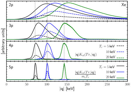
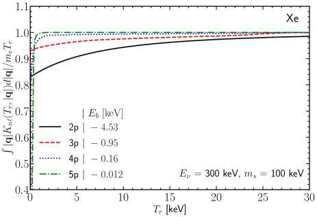
Figure 1: The left panel shows $|{\bf q}|K_{nl}(T_{r},|{\bf q}|)$ (dashed) and the phase space ratio $|{\bf q}|K_{nl}(T_{r},|{\bf q}|)/m_{e}T_{r}$ (solid) for the $2p$, $3p$, $4p$ and $5p$ orbitals from top to bottom. Three typical recoil energies $T_{r}=5\,$keV (black), 10 keV (blue), and $20\,$keV (green) are shown for illustration. The peak locations, $|{\bf q}|=\sqrt{2m_{e}T_{r}}$, estimated from the scattering with a free electron are shown as vertical gray lines. As a function of the electron recoil energy $T_{r}$, the right panel shows the phase space ratio $\int|{\bf q}|K_{nl}(T_{r},|{\bf q}|)d|{\bf q}|/m_{e}T_{r}$ for the $2p$ (black solid), $3p$ (red dashed), $4p$ (blue dotted) and $5p$ (green dash-dotted) orbitals in the Xe atom with solar neutrino energy $E_{\nu}=300$ keV and the sterile neutrino mass $m_{s}=100$ keV.

with $|{\bf p}|^{2}=2m_{e}T_{r}$. For easy comparison, we have kept the momentum transfer integration which can be removed by the $\delta(|{\bf p}|-|{\bf q}|)$ function. Comparing (16) with (13), we can see that the $K$-factor reduces to $|{\bf q}|\delta(|{\bf p}|-|{\bf q}|)/2$ in the free electron scattering limit. For the scattering with a free electron, the two-body phase space reduces to a single integration over either the recoil energy $T_{r}$ or equivalently the momentum transfer $|{\bf q}|$. But for the bound electron case, the phase space has double integration, over $T_{r}$ and $|{\bf q}|$ which are no longer correlated. This is because the initial bound electron does not have definite momentum but a distribution. Consequently, the contribution from different momentum transfer should be integrated. Besides $\overline{|\mathcal{M}|^{2}}/32\pi m^{2}_{e}|{\bf p}_{\nu}|^{2}T_{r}$, the phase space integrations are $m_{e}T_{r}$ and $\int|{\bf q}|K_{nl}(T_{r},|{\bf q}|)d|{\bf q}|$ for the free and bound electron cases, respectively. Assuming constant $|\mathcal{M}|^{2}$, the atomic enhancement can be roughly measured by the ratio between the phase space integrations, $\int|{\bf q}|K_{nl}(T_{r},|{\bf q}|)d|{\bf q}|/m_{e}T_{r}$.

The left panel of Fig. 1 shows the atomic factor $|{\bf q}|K_{nl}(T_{r},|{\bf q}|)$ (dashed) and the atomic factor ratio $|{\bf q}|K_{nl}(T_{r},|{\bf q}|)/m_{e}T_{r}$ (solid) as functions of the momentum transfer $|{\bf q}|$. The curves are narrower for outer shell electrons (larger $n$) and the typical width keeps growing when $n$ becomes smaller. The half width at the half height $\sigma_{|{\bf q}|}=(50,20,10,4)$  keV for the ($2p$, $3p$, $4p$, $5p$) electron can be directly read off from the solid lines. The solid and dashed lines share the same width since the only difference between them is a constant factor. For given electron shell, the width is independent of $T_{r}$. The width is exactly a manifestation of the electron motion inside atom. Pointing in all directions, the initial electron momentum smears the momentum transfer $|{\bf q}|$ and hence the recoil energy $T_{r}$. The larger initial momentum, the larger smearing effect. With binding energy $|E_{b}|=(4.53,0.95,0.16,0.012)$ keV for ($2p$, $3p$, $4p$, $5p$) orbitals Catena:2019gfa , the initial electron momentum can be estimated by non-relativistic dispersion relation, $|{\bf p}_{i}|\approx\sqrt{2m_{e}|E_{b}|}=$(68, 31, 13, 3.5) keV correspondingly. These numbers roughly match the width read off from the curves. Although the bound electron motion broadens the curves, the central values are largely unaffected, especially for the outer shells. The peak position can be estimated by the momentum transfer $|{\bf q}^{\rm peak}|\approx\sqrt{2m_{e}T_{r}}$ of the free electron scattering. For the three curves of $T_{r}=(5,10,20)$ keV, the estimated peak positions are $|{\bf q}^{\rm peak}|\approx(71,101,143)$ keV as indicated by three vertical grey lines from left to right. With larger $n$, the peak position becomes closer to the free electron momentum transfer.

The right panel of Fig. 1 shows the integrated phase space ratio as functions of the recoil energy $T_{r}$. The ratio starts from a relatively small value for vanishing $T_{r}$ and converges to $1$ with increasing $T_{r}$. This happens because for small $T_{r}$ the allowed momentum transfer is suppressed to have smaller phase space Essig:2011nj . In contrast, the electron approaches a free particle to have larger phase space with increasing $T_{r}$. For larger $n$, the integrated phase space ratio approaches $1$ faster, since the electron is less tightly confined to the atom.

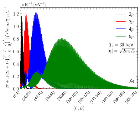
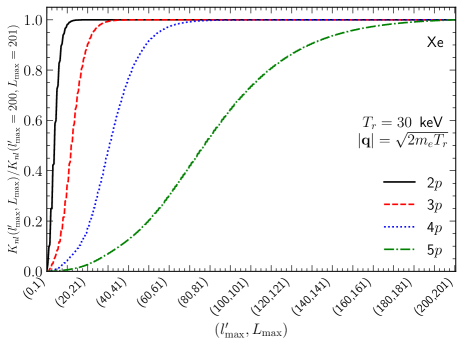
Figure 2: The left panel shows the non-zero terms of the double summation in (15) as a function of $l^{\prime},L$. The right panel shows the fraction between the partial sum for a given set of $l^{\prime}_{\rm max},L_{\rm max}$ and the total sum with $l^{\prime}_{\rm max}=200,L_{\rm max}=201$. In both cases, $T_{r}=30$ keV and $|{\bf q}|=\sqrt{2m_{e}T_{r}}$. The lines represents the 2p (black), 3p (red), 4p (blue) and 5p (green) orbitals in the Xe atom.

The left panel of Fig. 2 shows the non-zero terms inside the double summation of (15) as a function of the angular indices $(l^{\prime},L)$ for the $2p$, $3p$, $4p$, and $5p$ orbitals. Those terms violating $|l^{\prime}\pm L|=l$ are zero and omitted in the plot for simplicity. With increasing $n$, the peak shifts to the right. The $2p$ curve peaks around $l^{\prime}=5$ and drops to zero at $l^{\prime}=15$. For comparison, the $5p$ curve peaks around $l^{\prime}=95$ and is non-zero even for $l^{\prime}>190$. The exact evaluation of the $K_{nl}$ factor in (15) requires double summation over the principal quantum numbers, $l^{\prime}$ and $L$, to infinity which is highly time-consuming. To increase efficiency, we cut the summation at large enough $l^{\prime}_{\rm max}$ and $L_{\rm max}$ to guarantee precision.

The relative precision can be estimated from the right panel of Fig. 2. Each curve shows the ratio between the partial sum up to ($l^{\prime}_{\rm max}$, $L_{\rm max}$) divided by the one up to ($200$, $201$) for the $2p$, $3p$, $4p$, and $5p$ orbitals. With increasing ($l^{\prime}_{\rm max}$, $L_{\rm max}$), the ratio converges to 1. As $n$ increases, larger $l^{\prime}_{\rm max}$ and $L_{\rm max}$ are needed. For the $2p$, $3p$, $4p$, and $5p$ orbitals to achieve sub-percentage precision, ($l^{\prime}_{\rm max}$, $L_{\rm max}$) needs to be at least (10, 11), (30, 31), (70, 71), and (190, 191), respectively.

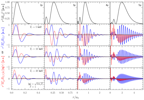
Figure 3: The oscillatory behavior in the bound and ionized electron wave functions. Each column stands for an individual initial electron level, $(nl)=2p$, $3p$, $4p$, and $5p$. The first row is purely for the initial electron radial wave function $r^{2}|R_{nl}|^{2}$ which appears in the integration for normalization. The next three rows are for the convolution between the initial and final electron radial functions $r^{2}R^{*}_{nl}R_{T_{r}l^{\prime}}$ (blue solid) and $r^{2}R^{*}_{nl}R_{T_{r}l^{\prime}}j_{L}(|{\bf q}|r)$ with $L=0$ (red dashed) for electron recoil energies $T_{r}=(5,10,20)$ keV. For illustration, we take the peak value $|{\bf q}|=\sqrt{2m_{e}T_{r}}$ of the momentum transfer. The horizontal axises are in the unit of Bohr radius $a_{0}=1/m_{e}\alpha$.

The integrand in (15) is highly oscillatory and illustrated in Fig. 3. The top panels show purely the initial bound electron wave functions as a convenient combination $r^{2}|R_{nl}|^{2}$ (black solid) that should appear in normalization integration. While the initial wave functions are quite regular with only one major peak, the final ionized electron wave functions oscillate a lot. This oscillatory behavior clearly appears in the product combination $r^{2}R^{*}_{nl}R_{T_{r}l^{\prime}}$ (blue solid). Since the bound and ionized states are orthogonal to each other, the product oscillates symmetrically around the vanishing value so that the integration should also vanish. The third component, the Bessel function $j_{L}(|{\bf q}|r)$, enters the atomic form factor to render a nonzero $K$-factor (15). The full combination $r^{2}R^{*}_{nl}R_{T_{r}l^{\prime}}j_{L}(|{\bf q}|r)$ (red dashed) has asymmetric oscillation so that its integration can be nonzero. With larger $n$, $l$, and $T_{r}$, the oscillation becomes more frequent. To accurately perform the integration in (15), a large number of grid points over $r$ is necessary. A sub-percentage precision requires $3000$ grid points in the range $r\in[0,10a_{0}]$ where $a_{0}\equiv 1/m_{e}\alpha$ is the Bohr radius.

III Neutrino Scattering into A Massive Sterile Neutrino with Light Mediators

With the second quantization formalism for the atomic effect established in the previous section, we can proceed to calculate the recoil spectrum (13) by implementing the concrete scattering matrix element $\overline{|\mathcal{M}|^{2}}$ as input from the particle physics side. For the solar neutrino scattering into a massive sterile neutrino in the final state, we first derive the differential cross section in Sec. III.1 and then show the modification due to atomic effects in Sec. III.2.

III.1 Neutrino Scattering with Free or Bound Electrons

The XENON1T excess in the low energy region can be explained by the solar neutrino scattering with electron via a scalar or pseudo-scalar mediator Ge:2020jfn .

$$\mathcal{L}_{\mathrm{int}}\equiv\bar{\nu}\left(y_{S}^{\nu}+\gamma_{5}y_{P}^{\nu}\right)\phi\nu_{s}+\bar{e}\left(y_{S}^{e}+\gamma_{5}y_{P}^{e}\right)e\phi+h.c.$$ (17)

In addition to the recoil electron, a massive sterile neutrino appears in the final state. For the scattering with a free electron, the cross section is a function of the recoil energy $T_{r}$,

Scalar $$: \frac{d\sigma^{0}_{S}}{dT_{r}}=\frac{(y^{\nu}_{S}y^{e}_{S})^{2}(2m_{e}+T_{r})}{8\pi E_{\nu}^{2}}\frac{2m_{e}T_{r}+m^{2}_{s}}{(2m_{e}T_{r}+m^{2}_{\phi})^{2}},$$ (18a)

Pseudo-Scalar $$: \frac{d\sigma^{0}_{P}}{dT_{r}}=\frac{(y^{\nu}_{P}y^{e}_{P})^{2}T_{r}}{8\pi E_{\nu}^{2}}\frac{2m_{e}T_{r}+m^{2}_{s}}{(2m_{e}T_{r}+m^{2}_{\phi})^{2}},$$ (18b)

In addition to the neutrino energy $E_{\nu}$, $m_{s}$ and $m_{\phi}$ are the sterile neutrino and scalar/pseudo-scalar mediator masses, respectively. Contrary to the common expectations Boehm:2020ltd with massless neutrinos, a massive sterile and a light mediator ($m^{2}_{\phi}\ll 2m_{e}T_{r}\ll m^{2}_{s}$) can introduce $1/T_{r}$ enhancement even for the pseudo-scalar mediator Ge:2020jfn by a factor of $m^{2}_{s}/2m_{e}T_{r}$. For a low energy electron recoil signal, such as the XENON1T excess at $T_{r}\approx(2\sim 3)\,\mbox{keV}$, the mediator mass should satisfy an upper bound $m_{\phi}\ll(45\sim 55)\,\mbox{keV}$ to receive enhancement.

For the scattering with a bound electron, the electron part resembles the free case for the scalar-type vertex and receives a momentum insertion for the pseudo-scalar one as shown in (11),

$$\overline{|{\mathcal{M}}_{S}|^{2}} = \frac{(y^{\nu}_{S}y^{e}_{S})^{2}}{2(q^{2}-m_{\phi}^{2})^{2}}\mbox{Tr}[\not{p}_{\nu}(\not{p}_{\nu_{s}}+m_{s})]\mbox{Tr}[(\not{p}_{e}+m_{e})(\not{p}^{\prime}_{e}+m_{e})],$$ (19a)

$$\overline{|{\mathcal{M}}_{P}|^{2}} = \frac{(y^{\nu}_{P}y^{e}_{P})^{2}}{2(q^{2}-m_{\phi}^{2})^{2}}\frac{1}{4m_{e}^{2}}\mbox{Tr}[\not{p}_{\nu}\gamma_{5}(\not{p}_{\nu_{s}}+m_{s})\gamma_{5}]\mbox{Tr}[(\not{p}_{e}+m_{e})({\bf q}\cdot\boldsymbol{\gamma})\gamma_{5}(\not{p}^{\prime}_{e}+m_{e})({\bf q}\cdot\boldsymbol{\gamma})\gamma_{5}].$$ (19b)

When calculating the trace, we should remember that the spinor for electron $u(m_{e})$ is the one without momentum. But it does not mean this approximation has no information of the electron momentum. Actually, the electron momentum appears as the gradient operator in (4), which when acting on the integration will generate the momentum transfer ${\bf{q}}$. This is also the origin of $\textbf{q}\cdot\boldsymbol{\gamma}$ in the pseudo-scalar matrix element. Putting the scalar and pseudo-scalar cases together, the spin-averaged matrix element is,

$$\overline{|\mathcal{M}_{S,P}|^{2}}=2\left(4m_{e}^{2}|y^{\nu}_{S}y^{e}_{S}|^{2}+|{\bf q}|^{2}|y^{\nu}_{P}y^{e}_{P}|^{2}\right)\frac{|{\bf q}|^{2}+m^{2}_{s}-\Delta E^{2}_{nl}}{(|{\bf q}|^{2}+m^{2}_{\phi}-\Delta E^{2}_{nl})^{2}}.$$ (20)

Although derived for the bound electron case, (20) can reproduce the leading terms of the free electron case (18) with the following replacements. The initial electron is at rest and the energy difference is exactly the recoil kinetic energy, $\Delta E_{nl}=T_{r}$, of the final electron. In addition, the momentum transfer magnitude $|{\bf q}|$ is uniquely related to the recoil energy, $|{\bf q}|^{2}=T^{2}_{r}+2m_{e}T_{r}$, due to the on-shell condition of the final-state electron.

On the other hand, a bound electron in the initial state has no definite momentum. There is no way to use the on-shell condition for the final-state ionized electron to correlate the energy change $\Delta E_{nl}\equiv T_{r}-E_{nl}$ and the momentum transfer magnitude $|{\bf q}|$. The differential cross section (13) is then an integration over all the possible momentum transfers,

$${\rm Scalar} : \frac{d\sigma^{nl}_{S}}{dT_{r}}=\frac{(y^{\nu}_{S}y^{e}_{S})^{2}}{4\pi E_{\nu}^{2}T_{r}}\int|{\bf q}|d|{\bf q}|\frac{|{\bf q}|^{2}+m^{2}_{s}-\Delta E^{2}_{nl}}{(|{\bf q}|^{2}+m^{2}_{\phi}-\Delta E^{2}_{nl})^{2}}K_{nl}(T_{r},|{\bf q}|),$$ (21a)

Pseudo-Scalar $$: \frac{d\sigma^{nl}_{P}}{dT_{r}}=\frac{(y^{\nu}_{P}y^{e}_{P})^{2}}{4\pi E_{\nu}^{2}T_{r}}\int|{\bf q}|d|{\bf q}|\frac{|{\bf q}|^{2}}{4m_{e}^{2}}\frac{|{\bf q}|^{2}+m^{2}_{s}-\Delta E^{2}_{nl}}{(|{\bf q}|^{2}+m^{2}_{\phi}-\Delta E^{2}_{nl})^{2}}K_{nl}(T_{r},|{\bf q}|).$$ (21b)

The similar scenario with a light vector boson mediator can also explain the XENON1T excess Ge:2020jfn . For simplicity, we consider only the situation where $Z^{\prime}$ couples to the left-handed neutrino,

$$\mathcal{L}_{\text{int }}\equiv g_{L}^{\nu}\bar{\nu}\gamma^{\mu}P_{L}\nu_{s}Z_{\mu}^{\prime}+\bar{e}\left(g_{V}^{e}-g_{A}^{e}\gamma_{5}\right)\gamma^{\mu}eZ_{\mu}^{\prime},$$ (22)

while the electron coupling can have either vector ($g^{e}_{V}$) or axial-vector ($g^{e}_{A}$) current coupling with $Z^{\prime}$. The differential cross section of neutrino scattering with a free electron is,

$$\frac{d\sigma^{0}_{V,A}}{dT_{r}}=\frac{\left(g_{L}^{\nu}g_{V,A}^{e}\right)^{2}}{4\pi E_{\nu}^{2}}\frac{4m_{e}E^{2}_{\nu}-(2m_{e}T_{r}+m^{2}_{s})(2E_{\nu}\pm m_{e}-T_{r})}{\left(2m_{e}T_{r}+m_{Z^{\prime}}^{2}\right)^{2}},$$ (23)

where the $+\,(-)$ signs are for the vector and axial-vector interactions, respectively. The sterile neutrino mass term $m^{2}_{s}$ and hence the second term in the numerator can be important only when $m_{s}$ becomes comparable with the electron mass $m_{e}$ and the neutrino energy $E_{\nu}$. In this paper, we focus on the mass region $m_{s}\sim\mathcal{O}(100)$ keV. Then with $4m_{e}E^{2}_{\nu}$ dominating the numerator, a $1/T^{2}_{r}$ enhancement is possible for a light enough mediator, $m^{2}_{Z^{\prime}}\ll 2m_{e}T_{r}$. For comparison, the differential cross section of neutrino scattering with a bound electron is,

$$\frac{d\sigma_{V,A}^{nl}}{dT_{r}}=\frac{(g^{\nu}_{L}g^{e}_{V,A})^{2}}{4\pi E_{\nu}^{2}T_{r}}\int|\boldsymbol{q}|d|\boldsymbol{q}|\frac{4E_{\nu}(E_{\nu}-\Delta E_{nl})\mp(|\boldsymbol{q}|^{2}+m_{s}^{2}-\Delta E^{2}_{nl})}{(|\boldsymbol{q}|^{2}+m_{Z^{\prime}}^{2}-\Delta E^{2}_{nl})^{2}}K_{nl}(T_{r},|{\bf q}|),$$ (24)

with $\mp$ for the vector and axial-vector couplings, respectively.

III.2 The Cross Section Enhancement from Atomic Effects

By implementing the $K$-factor elaborated in Sec. II.2, we obtain the differential cross sections (21) and (24) for scalar and vector mediators. To see the features clearly, we first evaluate $d\sigma^{nl}/dT_{r}$ for the transition of a single initial electron in a given $nl$ bound state to the ionized electron with recoil energy $T_{r}$, shown as colorful lines in Fig. 4. For comparison, we also show the free electron case as black solid line. We take the scalar and pseudo-scalar mediators to illustrate the physics picture while the vector case is similar.

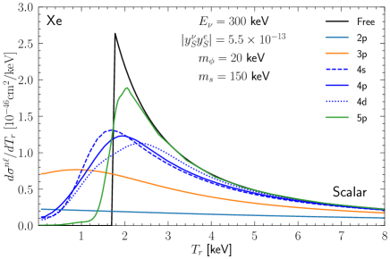
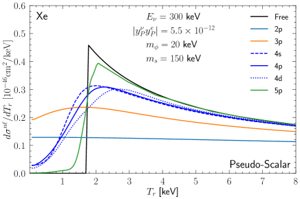
Figure 4: The differential cross section of $\nu$-$e$ scattering with a massive sterile neutrino in the final state and light scalar (left) or pseudo-scalar (right) mediator. The black line is for the scattering with a free electron while the colorful lines are for the bound electrons $2p$ (solid cyan), $3p$ (solid yellow), $4s$ (dashed blue), $4p$ (solid blue), $4d$ (dotted blue), and $5p$ (solid green) of a Xenon atom. In both subplots, the final-state sterile neutrino mass is $m_{s}=150$ keV and the mediator mass is $m_{\phi}=20$ keV.

The difference is quite significant. Especially, the smearing effect makes the sharp peak much fatter and lower mainly due to the electron motion in the atom. For smaller principal quantum number $n$, the reduction is much stronger. One reason is the phase space ratio due to the atomic $K$-factor as shown in Fig. 1. Another factor comes from the scattering matrix element. The electron in the atomic Coulomb potential has a negative binding energy $E_{b}$ which is exactly $E_{nl}$. Intuitively, It is more difficult for an electron with larger binding energy to be recoiled off. If the energy change $\Delta E_{nl}=T_{r}-E_{nl}$ in (20) dominates, especially for the inner shells, the scattering matrix element can be greatly suppressed. This is because the momentum transfer peaks at $|{\bf q}|=\sqrt{2m_{e}T_{r}}$ with large spread above the peak position as shown in Fig. 1. So the modification of the differential cross section is a combined result of the $K$-factor phase space integration reduction and the scattering matrix element suppression. On the other hand, the electron in outer shells is loosely trapped with marginal suppression and is very similar to the free case.

In addition, the smearing effect extends the spectrum beyond the cut-off. For free electron scattering, the recoil energy is bounded from below, $T_{r}\geq T^{-}_{r}$ as defined in our earlier paper Ge:2020jfn . A nonzero lower limit $T^{-}_{r}\approx m^{4}_{s}/8m_{e}E^{2}_{\nu}$ arises when expanding the sterile neutrino mass to the fourth power. For the $E_{\nu}=300\,$keV used to plot the black solid line, the differential cross section vanishes around $1.7$ keV. However, bound electrons have distributed momentum in all directions and hence can smear the momentum transfer to extend the recoil energy $T_{r}$ even down to $0\,$keV. Furthermore, the $2p$ or $3p$ electrons even have a non-zero differential cross section at vanishing $T_{r}$. As shown in (13), the phase space integration is $|{\bf q}|d|{\bf q}|$. Since the lower limit $E_{\nu}-\sqrt{(E_{\nu}-\Delta E_{nl})^{2}-m^{2}_{s}}$ of $|{\bf q}|$ with $\Delta E_{nl}>0$ is always nonzero for the scattering of bound electron into an ionized one, the phase space would not disappear even for $T_{r}=0$ keV. This behavior can also explain the sudden drop of the $5p$ curve when approaching vanishing $T_{r}$ in Fig. 1.

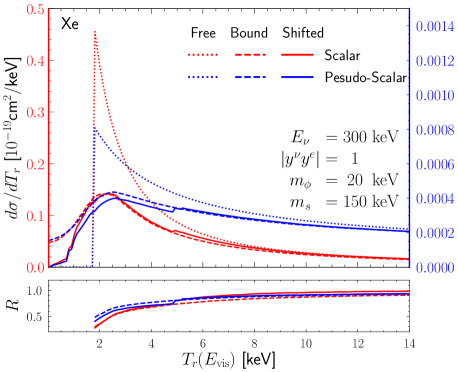
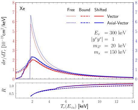
Figure 5: The differential cross section of neutrino scattering with all electrons of Xe atom into a massive sterile neutrino. The left panel shows the case with scalar (red) and pseudo-scalar (blue) mediators. For comparison, we also show the vector mediator case in the right panel with vector (red) and axial vector (blue) couplings. Both panels show the results with free (dotted), bound (dashed), and the shifted one including recombination energies (solid). The enhancement from the free electron scattering cross section is shown as ratio $R$ in the lower panels for comparison. Since the couplings only appear as overall factor, we adopt $|y^{\nu}y^{e}|=|g^{\nu}g^{e}|=1$ for simplicity.

Solar neutrino can scatter with electrons of different quantum numbers inside the Xenon atom. For the free electron scattering, the total $d\sigma/dT_{r}$ is simply $N_{e}=54$ times of the differential cross section for a single electron where $N_{e}$ is the electron number in the Xenon atom. The total cross section for the bound electron scattering is a sum over all the differential cross sections $d\sigma^{nl}/dT_{r}$,

$$\mbox{Free}~{}:~{}\frac{d\sigma}{dT_{r}}=54\times\frac{d\sigma^{0}}{dT_{r}},\quad{\rm vs}\quad\mbox{Bound}~{}:~{}\frac{d\sigma_{A}}{dT_{r}}=\sum_{nl}2(2l+1)\frac{d\sigma^{nl}}{dT_{r}}.$$ (25)

Of the weight $2(2l+1)$, the factor 2 for the bound case accounts for the two electron spin degrees of freedom with the same $nlm$ quantum numbers. Note that the summation over the magnetic quantum number $m$ results in the $2l+1$ factor. As illustrated by the blue lines in Fig. 4, the $4s$, $4p$, and $4d$ curves with the same principal quantum number $n=4$ but different angular quantum numbers have similar shapes and amplitudes. More generally, orbitals with the same principal quantum number have roughly the same differential cross sections. The $n=5$ orbitals have higher and sharper peaks than the $n=4$ ones. However, the electron number of the former, $2(5s)+6(5p)=8$, is less than half of the later, $2(4s)+6(4p)+10(4d)=18$. So the total differential cross section of atomic scattering (thick dashed and solid) in Fig. 5 is mainly contributed by the $4s$, $4p$, and $4d$ curves (blue) in Fig. 4. Since the differential cross section $d\sigma^{nl}/dT_{r}$ for a single electron is reduced for all $nl$ quantum numbers, the total result $d\sigma_{A}/dT_{r}$ is also reduced from the free electron case. As shown in the lower panel, the reduction is roughly a factor of 0.5 in the low-energy region ($T_{r}\lesssim 5$ keV) and gradually recovers to 1 in the high energy region ($T_{r}\gtrsim 10$ keV) for the scalar or pseudo-scalar mediators. For vector and axial-vector interactions, atomic effects bring the same features.

A key difference between the scalar/pseudo-scalar and vector/axial-vector interactions is that the latter has much larger cross section by almost a factor of $10\sim 15$, as shown in the upper panels of Fig. 5. As discussed below (23), the matrix element part is approximately $4m_{e}E_{\nu}^{2}/(2m_{e}T_{r}+m^{2}_{Z^{\prime}})^{2}$ for the free electron scattering with vector mediator. For comparison, the scalar case has $m_{e}(2m_{e}T_{r}+m^{2}_{s})/(2m_{e}T_{r}+m^{2}_{\phi})^{2}$. With tiny mediator mass, $m^{2}_{\phi},m^{2}_{Z^{\prime}}\ll 2m_{e}T_{r}$, the difference mainly comes from the numerator part. The ratio between vector and scalar matrix elements is $4m_{e}E_{\nu}^{2}/m_{e}(2m_{e}T_{r}+m^{2}_{s})$. We can see that the vector case has a major contribution $4m_{e}E^{2}_{\nu}$. With $E_{\nu}\approx 300$ keV, $m_{s}\approx 150$ keV, and $|{\bf q}|^{2}\sim 2m_{e}T_{r}\approx 3000$ keV, the vector cross section is naturally enhanced by a factor around 10.

In addition to the free (dotted) and bound (dashed) electron curves, Fig. 5 also shows the shifted results. This is because the energy deposit $\Delta E_{nl}$ is not just the electron recoil energy $T_{r}$ but also the binding energy $E_{b}=E_{nl}$. The later is released when an ambient electron is attracted by the positively charged Xenon atom to fill the hole left by the ionized electron Szydagis:2011tk . The differential cross section is then shifted to the right as the solid lines. The binding energy is typically $\mathcal{O}(0.01)$ keV for outer shells Szydagis:2011tk and can be ignored in comparison to the recoil energy. But the binding energy can be as large as $\mathcal{O}(10)$ keV for most inner shells and hence seems able to induce significant horizontal shift, the differential cross section $d\sigma^{nl}/dT_{r}$ is suppressed by the same large binding energy in the first place as discussed above. So the energy shift does not affect the total differential cross section $d\sigma/dE_{\rm vis}$ much as shown in the plot.

IV Experimental Constraints

The XENON1T Collaboration has recently observed an excess in the electron recoil spectrum around $(2\sim 3)$ keV Aprile:2020tmw . The experimental data is shown as black points in Fig. 6 while the total background from radioactive materials present in the detector and solar neutrino scattering is shown as the red curve for comparison. Note that the background is roughly flat and hence can not explain the excess at low energy. It is possible for this excess to arise from some new physics and the data points can be used to constrain the possible new physics model parameters.

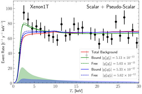
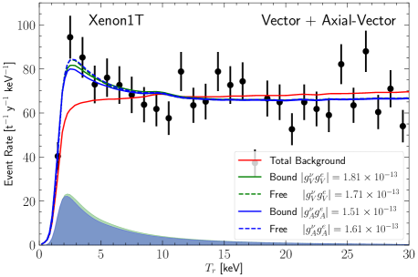
Figure 6: Total events (black points) and background (red curve) of XENON1T’s data, we fit the data by solar neutrino-bound electron scattering with a sterile neutrino in final state, in addition to both scalar (green) and pseudo scalar(blue) mediators. All three parameters $m_{s},m_{\phi},|y_{e}y_{p}|$ are using the best-fitting values.

In this paper, we give a more detailed evaluation of the constraint on the solar neutrino scattering with electrons into a massive sterile neutrino Ge:2020jfn . The atomic effects are also included to give a realistic result. We use the following $\chi^{2}$ function,

$$\chi^{2}\equiv\sum_{i}^{\rm bins}\left(\frac{N^{\rm data}_{i}-(1+c)N^{\rm bkg}_{i}-N^{\rm NP}_{i}}{\sqrt{N^{\rm data}_{i}}}\right)^{2}+\left(\frac{c}{\sigma}_{c}\right)^{2},$$ (26)

to evaluate the best-fit value and sensitivities. The $\chi^{2}$ function contains two major contributions: the first term from the data bins and the second is nuisance parameter $c$ for the background normalization with uncertainty $\sigma_{c}=2.6\%$ Aprile:2020tmw . In each bin, $N^{\rm data}_{i}$ is the data point, $N^{\rm bg}_{i}$ the expected background, and $N^{\rm NP}_{i}$ the expected events due to new physics (NP) contribution. For the light mediator case considered in this paper, $N^{\rm NP}_{i}$ is a function of the mediator mass ($m_{\phi}$ or $m_{Z^{\prime}}$), the sterile neutrino mass ($m_{s}$), and couplings ($|y^{\nu}_{S,P}y^{e}_{S,P}|$ or $|g^{\nu}_{V,A}g^{e}_{V,A}|$).

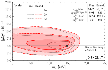
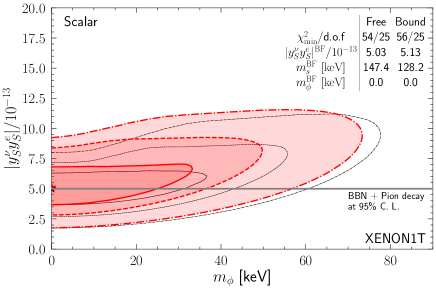
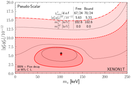
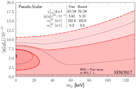
Figure 7: The XENON1T constraints for scalar (up), pseudo-scalar (bottom) interaction couplings $|y_{S,P}^{\nu}y_{S,P}^{e}|$ versus $m_{s}$ (left) and $m_{\phi}$ (right) at $1\sigma$, $2\sigma$, and $3\sigma$ C.L. The black curves are for the free electron approximation and red ones for the bound electron scenario whose best-fit points are indicated with black (free) and red (bound) stars, respectively. The mediator (sterile neutrino) mass $m_{\phi}$ ($m_{s}$) is marginalized over $0\,\mbox{keV}<m_{\phi}<175$ keV ($0\,\mbox{keV}<m_{s}<250$ keV).

On the theoretical side, the event rates are calculated by the convolution of the differential cross-section defined in (25) and the solar neutrino flux. We use the $pp$-neutrinos since they have the largest flux at low energy Vinyoles:2016djt . The detector’s energy resolution is also taken into account by a Gaussian parametrization with variance given by $\sigma_{T_{r}}=a/\sqrt{T_{r}/{\rm keV}}+b$ with $a=31.71\pm 0.65\,$keV and $b=0.15\pm 0.02\,$keV Aprile:2020yad . In addition, the detector efficiency at a given recoil energy $T_{r}$ is extracted from Aprile:2020tmw . Fig. 7 shows the best-fit values and exclusion curves obtain by fitting the predicted event numbers $N^{\rm NP}_{i}$ with data using (26). The left and right panels are obtained by fixing two parameters, $|y^{\nu}_{S,P}y^{e}_{S,P}|$ and $m_{\phi}$ ($m_{s}$), and minimizing the $\chi^{2}$ function over the remaining $m_{s}$ ($m_{\phi}$).

For comparison, each panel shows both free (black curves) and bound (red areas) electron scenarios. The bound-to-free ratio $R=0.5$ for the scalar mediator in Fig. 5 seems be quite different from 1 and can have significant consequence. However, it is mainly due to the broadening effect of the electron motion inside atom. With detector smearing effect, the sharp peak for the free scattering case would also become broader and lower to more closely resemble the bound case. Consequently, the coupling best-fit value almost does not change. Take the scalar interaction as an example, the coupling best fit marginally shifts from the free electron case ($|y^{e}_{S}y^{\nu}_{S}|=5.03\times 10^{-13}$) to the bound one, $|y^{e}_{S}y^{\nu}_{S}|=5.13\times 10^{-13}$. Similarly, the coupling strength changes from $5.63\times 10^{-12}$ to $5.33\times 10^{-13}$ for pseudo-scalar mediator. The background-only hypothesis ($|y^{e}_{S,P}y^{\nu}_{S,P}|=0$) is excluded by more than $3\sigma$ C.L. for the scalar interaction but is still inside the $2\sigma$ region for the pseudo-scalar case. This is because the pseudo-scalar interaction has a smooth total differential cross section (blue curves in the left panel of Fig. 5) and is not as different from the background as the scalar one.

In addition to the DM direct detection, the coupling with electron $y^{e}_{S,P}$ also receives constraints from other experiments and astrophysical observations. The torsion balance experiments impose a constraint $|y^{e}_{S,P}|<10^{-23}$ at 95% C.L. for the mediator mass below $4\times 10^{-6}$ eV Adelberger:2009zz , which is 10 orders smaller than the current DM direct detection constraints of $\mathcal{O}(10^{-13}$). In other words, an ultra-light mediator cannot explain the XENON1T excess. The mediator mass up to $\mathcal{O}(0.01)$ eV is also excluded by the Red Giant (RG) and Horizontal Branch (HB) stellar cooling constraint $|y^{e}_{S,P}|<10^{-16}$ Hardy:2016kme at 95% C.L. that is 3 orders smaller than the DM direct detection ones. The Big Bang nucleosynthesis (BBN) constrains the mediator mass above $10^{-2}$ eV. The $\phi$ production in the early Universe increases the relativistic degrees of freedom and accelerates the universe expansion. A faster expansion reduces the deuterium abundance. The $\phi$ production can only be evaded if $|y^{e}_{S,P}|<5\times 10^{-10}$ at 95% C.L. or $m_{\phi}>1$  MeV Babu:2019iml . For the coupling with neutrino, the meson decay experiments require $|y_{S,P}^{\nu}|\lesssim 10^{-3}$ if $m_{s}<m_{\pi}$ Pasquini:2015fjv ; Berryman:2018ogk ; Dror:2020fbh ; deGouvea:2019qaz . Altogether, the combined constraint is $|y^{e}_{S,P}y^{\nu}_{S,P}|\lesssim 5\times 10^{-13}$ in the mass region $m_{\phi}>10^{-2}$ eV (the gray lines in Fig. 7). The best-fit value of the scalar case is allowed while the pseudo-scalar one is in tension.

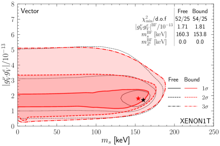
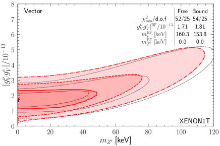
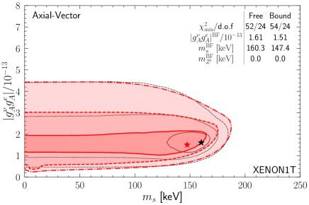
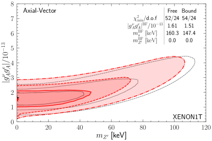
Figure 8: The XENON1T constraints for vector (up), axial-vector (bottom) interaction couplings $|g_{V,A}^{\nu}g_{V,A}^{e}|$ versus $m_{s}$ (left) and $m_{\phi}$ (right) at $1,2$ and $3\sigma$ C.L. The same as before, black curves are for free electron approximation and red ones for bound electron scenario. Their best-fit values are indicated with black (free) and red (bound) stars. The mediator (sterile neutrino) mass $m_{Z^{\prime}}$ ($m_{s}$) is marginalized over $0\,\mbox{keV}<m_{Z^{\prime}}<175$ keV ($0\,\mbox{keV}<m_{s}<250$ keV).

The best-fit value of sterile neutrino mass almost does not change for the scalar interaction, the best fit shifts slightly from $m_{s}=147.4$ keV to $128.2$ keV after implementing atomic effects. For the pseudo-scalar interaction, the best fit remains almost the same at $m_{s}=102.6$ keV. In other words, the dependence on the sterile neutrino mass is not sensitive to the atomic effects. Similar feature also applies for the light mediator mass whose best-fit value is 0 keV in all situations. This is because the propagator contribute a factor $\propto 1/(|\textbf{q}|^{2}-\Delta E^{2}_{nl}+m_{\phi}^{2})^{2}$ in the differential cross section which typically grows with decreasing $m_{\phi}$ for given $|{\bf q}|^{2}$. In other words, a smaller mediator mass leads to a higher peak at lower recoil energy which is preferred by the XENON1T data. However, the light mediator mass cannot really be zero due to various constraints Babu:2019iml ; Adelberger:2009zz . To be on the safe side, we adopt $m_{\phi}=10$ keV which is still inside the $1\sigma$ range when predicting the event rates in Sec. V. A mediator mass of 10 keV avoids the constraints mentioned before. This modification does not make big difference in the direct detection measurement. To be more concrete, the $\chi^{2}$ only increases by 1 and 1.5 for the scalar and pseudo-scalar cases, respectively.

Fig. 8 shows the results for vector and axial-vector interactions. We can see that the basic features are similar to the scalar and pseudo-scalar counterparts. The coupling $|g_{V}^{\nu}g_{V}^{e}|$ changes from $1.7\times 10^{-13}$ to $1.8\times 10^{-13}$ for vector while $|g_{A}^{\nu}g_{A}^{e}|$ changes from $1.6\times 10^{-13}$ to $1.5\times 10^{-13}$ for axial vector interactions. This change can also be understood by the combination of bound-to-free cross section ratio and the detector smearing effect in a similar way as the scalar/pseudo-scalar cases above. Both vector and axial-vector interactions can exclude the background-only hypothesis by more than $3\sigma$. The best-fit value of sterile neutrino mass is around $150$ keV and the mediator mass still prefers a tiny value. Similarly to the scalar and pseudo-scalar cases, we take $m_{Z^{\prime}}=10$ keV below when making projections for the future experiments.

The most stringent model-independent constraint on the coupling with electron, $|g^{e}_{V,A}|<5\times 10^{-10}$, also comes from BBN Ibe:2020dly . In the sterile neutrino mass region $m_{s}<m_{\pi}$, the leptonic pion decay imposes a bound $|g^{\nu}_{V,A}|<0.014$ on the coupling with neutrino Bakhti:2017jhm ; Dror:2020fbh . The combined result is $|g^{e}_{V,A}g^{\nu}_{V,A}|<7\times 10^{-12}$. For both the vector and axial-vector interactions, the best-fit points are well below this constraint. Both cases can escape the constraints. In fact, the bound is one order of magnitude higher than the best-fit points and is not visible in Fig. 8

V Predictions for Future DM Experiments

Although the XENON1T excess can be explained by new physics, the significance is not large enough and there is still no definite conclusion for the DM-electron interaction Aprile:2020tmw . Especially, the tritium background is also possible explanation Aprile:2020tmw ; PandaX-II:2020udv . More data is necessary to obtain a conclusive result. In this section, we use the best-fit values from the current XENON1T data to make prediction for future experiments.

We focus on three major DM direct detection experiments with liquid Xenon target. First, the PandaX-4T experiment Zhang:2018xdp that has already started running in 2021 is an upgrade of PandaX-II with a fiducial mass of 2.8 t and a factor of 10 improvement in the sensitivity. Next is the XENONnT experiment Aprile:2020vtw upgraded from XENON1T. XENONnT has a fiducial mass of 4 t and can reduce its background by a factor of 6. Finally, the LUX-Zeplin (LZ) experiment is a combination of two existing experiments LUX Akerib:2016vxi and Zeplin-III Akimov:2011tj . Its fiducial mass can reach 5.6 t and also has very low background. In addition, we make predictions with the same efficiency of PandaX-II Tan:2016zwf for PandaX-4T and XENON1T Aprile:2020tmw for XENONnT while for LZ the Fig. 3 of Akerib:2018lyp is used.

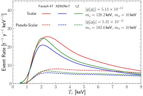
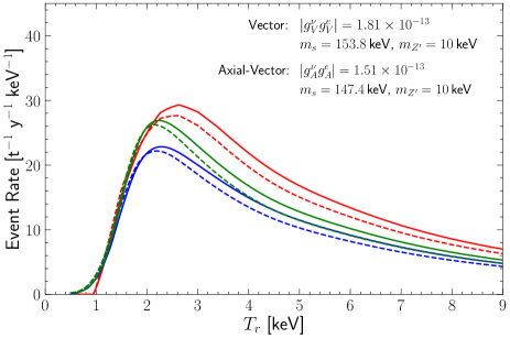
Figure 9: Predictions for three future experiments, PandaX-4T (red), XENONnT (blue), and LZ (green). left plot is for scalar (solid) and pseudo-scalar (dashed) interactions while right plot for vector (solid) and axial-vector (dashed) interactions.

Fig.9 shows the predicted event rates with atomic effects for future experiments PandaX-4T (red), XENONnT (blue), and LZ (green). The left panel shows the results for scalar (solid) and pseudo-scalar (dashed) interactions while the right panel shows the vector (solid) and axial-vector (dashed) cases. In these predictions, the couplings and the sterile neutrino mass $m_{s}$ are assigned the best-fit values with the XENON1T data. But the light mediator masses ($m_{\phi}$ and $m_{Z^{\prime}}$) take a universal value of 10 keV. With atomic effects, the event rates for scalar, vector and axial-vector interactions have a more conspicuous low energy excess around $(2\sim 3)$ keV. The event rate for the pseudo-scalar interaction gradually increases towards low energy.

Fig. 10 shows the expected sensitivity of the scalar, pseudo-scalar (left) and vector, axial-vector (right) couplings as function of the sterile neutrino mass $m_{s}$, for the three future DM experiments PandaX-4T, Lux-Zeplin, and XENONnT. Their nominal exposure are 5.6, 15.3, and 20 ton-years, respectively. The results represent a benchmark where the radioactivity background is reduced to a negligible level. Only the irreducible solar neutrino background is considered in the analysis. There is no new physics presenting in the pseudo data. For each $m_{s}$, we first fix $m_{\phi},m_{Z^{\prime}}=10$ keV to obtain a $\Delta\chi^{2}$ as function of the coupling constants. From this one-dimensional $\Delta\chi^{2}$, we obtain the 95% C.L. limit with $\Delta\chi^{2}=3.84$ on couplings as shown in Fig. 10.

The sensitivity varies among PandaX-4T, XENONnT, and Lux-Zeplin due to different exposure time of 2 years, 5 years, and 1000 days, respectively. All experiments can probe the best-fit values in Fig. 7 and Fig. 8. They can also improve the sensitivity by roughly one order of magnitude. For example, the best-fit value of pseudo-scalar interaction is $5.6\times 10^{-12}$ at XENON1T and the constraint becomes $\mathcal{O}(10^{-13})$ in Fig. 10. With this improvement, the future DM experiments can confirm or falsify the pseudo-scalar explanation to the XENON1T excess.

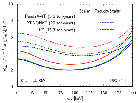
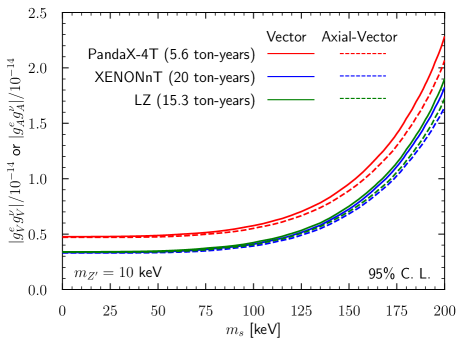
Figure 10: The PandaX-4T (red), XENONnT (blue), and Lux Zeplin (green) projected 95% C.L. exclusion curves as a function of the sterile neutrino mass $m_{s}$. The left panel is for the scalar (solid) and pseudo-scalar (dashed) mediators while the right panel is for the vector (solid) and axial-vector (dashed) interactions. In all cases, the mediator mass is fixed at $m_{\phi,Z^{\prime}}=10$ keV.

VI Conclusions

The XENON1T electron recoil excess stimulated various explanations with new physics including solar neutrino scattering with light mediators. Although the atomic effects are commonly considered for those dark matter scenarios, they are omitted in the solar neutrino explanations. In the first part of this work, we establish a systematic second quantization formalism for both the initial-state bound and final-state ionized electrons. This approach introduces the atomic $K$-factor in a natural way with general interactions for both neutrino and dark matter scatterings. The $K$-factor calculation includes a summation over the final-state angular quantum number $l^{\prime}$ to infinity. In practice, one needs to truncate the summation at some maximum value $l^{\prime}_{max}$ and this introduces some calculation error. A sub-percent precision in the atomic $K$-factor requires at least $l^{\prime}_{max}=200$ for the electron recoil energy of $\mathcal{O}(10)$ keV.

This formalism is then applied to the solar neutrino scattering with bound electrons into a sterile neutrino through scalar, pseudo-scalar, vector, and axial-vector interactions. The atomic effects decrease the cross section by $1\sim 5$ times to modify the recoil energy spectrum. Besides, the electron momentum distribution inside atom smears the momentum transfer of scattering. Consequently, the differential cross sections become smoother and broader than the free case. We then use the bound electron scattering scenario to fit the XENON1T excess. The scalar, vector, and axial-vector interactions are preferred over the background-only hypothesis by more than $3\sigma$ with best-fit coupling constants of $\mathcal{O}(10^{-13})$. Meanwhile, the pseudo-scalar case is favored over the background-only hypothesis by less than $2\sigma$ with a coupling constant of $\mathcal{O}(10^{-12})$. In all cases, the best-fit value of sterile neutrino mass is around $100$ keV. Our results demonstrate for the first time that the atomic effects can not be ignored when using solar neutrino scattering to explain the XENON1T electron recoil excess.

Finally, we project the signal event rate and sensitivity at PandaX-4T, XENONnT, and LZ. These future experiments improve the sensitivity by roughly one order. The current best-fit values and the $1\sigma$ C.L. regions of the scalar, vector, and axial-vector mediators are marginally below the constraints from astrophysics and pion decay. For the pseudo-scalar case, most regions of the parameter space are in tension with the current constraint. With a factor of $10$ improvement in sensitivity, the solar active-sterile neutrino conversion with bound electrons via light mediators as an explanation to the XENON1T excess can be tested.

References

- (1) M. Schumann, “Direct Detection of WIMP Dark Matter: Concepts and Status,” J. Phys. G 46, no.10, 103003 (2019) [arXiv:1903.03026 [astro-ph.CO]].
- (2) E. Aprile, et al., “Observation of Excess Electronic Recoil Events in XENON1T”, Phys. Rev. D 102 (2020) no.7, 072004 [arXiv:2006.09721] [hep-ex]
- (3) X. Zhou et al. [PandaX-II], “A search for solar axions and anomalous neutrino magnetic moment with the complete PandaX-II data,” doi:10.1088/0256-307X/38/1/011301
- (4) J. Jeong, J. E. Kim and S. Youn, “Electromagnetic properties of neutrinos from scattering on bound electrons in atom,” [arXiv:2105.01842 [hep-ph]].
- (5) A. E. Robinson, “XENON1T observes tritium,” [arXiv:2006.13278 [hep-ex]].
- (6) F. Takahashi, M. Yamada and W. Yin, “XENON1T Excess from Anomaly-Free Axionlike Dark Matter and Its Implications for Stellar Cooling Anomaly,” Phys. Rev. Lett. 125, no.16, 161801 (2020) [arXiv:2006.10035 [hep-ph]].
- (7) L. Di Luzio, M. Fedele, M. Giannotti, F. Mescia and E. Nardi, “Solar axions cannot explain the XENON1T excess,” Phys. Rev. Lett. 125, no.13, 131804 (2020) [arXiv:2006.12487 [hep-ph]].
- (8) C. Gao, J. Liu, L. T. Wang, X. P. Wang, W. Xue and Y. M. Zhong, “Reexamining the Solar Axion Explanation for the XENON1T Excess,” Phys. Rev. Lett. 125, no.13, 131806 (2020) [arXiv:2006.14598 [hep-ph]].
- (9) J. B. Dent, B. Dutta, J. L. Newstead and A. Thompson, “Inverse Primakoff Scattering as a Probe of Solar Axions at Liquid Xenon Direct Detection Experiments,” Phys. Rev. Lett. 125, no.13, 131805 (2020) [arXiv:2006.15118 [hep-ph]].
- (10) C. A. J. O’Hare, A. Caputo, A. J. Millar and E. Vitagliano, “Axion helioscopes as solar magnetometers,” Phys. Rev. D 102, no.4, 043019 (2020) [arXiv:2006.10415 [astro-ph.CO]].
- (11) C. Dessert, J. W. Foster, Y. Kahn and B. R. Safdi, “Systematics in the XENON1T data: The 15-keV anti-axion,” Phys. Dark Univ. 34, 100878 (2021) [arXiv:2006.16220 [hep-ph]].
- (12) T. Li, “The KSVZ Axion and Pseudo-Nambu-Goldstone Boson Models for the XENON1T Excess,” [arXiv:2007.00874 [hep-ph]].
- (13) P. Athron, C. Balázs, A. Beniwal, J. E. Camargo-Molina, A. Fowlie, T. E. Gonzalo, S. Hoof, F. Kahlhoefer, D. J. E. Marsh and M. T. Prim, et al. “Global fits of axion-like particles to XENON1T and astrophysical data,” JHEP 05, 159 (2021) [arXiv:2007.05517 [astro-ph.CO]].
- (14) C. Han, M. L. López-Ibáñez, A. Melis, O. Vives and J. M. Yang, “Anomaly-free leptophilic axionlike particle and its flavor violating tests,” Phys. Rev. D 103, no.3, 035028 (2021) [arXiv:2007.08834 [hep-ph]].
- (15) Y. Chen, M. Y. Cui, J. Shu, X. Xue, G. W. Yuan and Q. Yuan, “Sun heated MeV-scale dark matter and the XENON1T electron recoil excess,” JHEP 04, 282 (2021) [arXiv:2006.12447 [hep-ph]].
- (16) Q. H. Cao, R. Ding and Q. F. Xiang, “Searching for sub-MeV boosted dark matter from xenon electron direct detection,” Chin. Phys. C 45, no.4, 045002 (2021) [arXiv:2006.12767 [hep-ph]].
- (17) L. Su, W. Wang, L. Wu, J. M. Yang and B. Zhu, “Atmospheric Dark Matter and Xenon1T Excess,” Phys. Rev. D 102, no.11, 115028 (2020) [arXiv:2006.11837 [hep-ph]].
- (18) G. Paz, A. A. Petrov, M. Tammaro and J. Zupan, “Shining dark matter in Xenon1T,” Phys. Rev. D 103, no.5, L051703 (2021) [arXiv:2006.12462 [hep-ph]].
- (19) K. Nakayama and Y. Tang, “Gravitational Production of Hidden Photon Dark Matter in Light of the XENON1T Excess,” Phys. Lett. B 811, 135977 (2020) [arXiv:2006.13159 [hep-ph]].
- (20) Y. Jho, J. C. Park, S. C. Park and P. Y. Tseng, “Leptonic New Force and Cosmic-ray Boosted Dark Matter for the XENON1T Excess,” Phys. Lett. B 811, 135863 (2020) [arXiv:2006.13910 [hep-ph]].
- (21) L. Zu, G. W. Yuan, L. Feng and Y. Z. Fan, “Mirror Dark Matter and Electronic Recoil Events in XENON1T,” Nucl. Phys. B 965, 115369 (2021) [arXiv:2006.14577 [hep-ph]].
- (22) L. Delle Rose, G. Hütsi, C. Marzo and L. Marzola, “Impact of loop-induced processes on the boosted dark matter interpretation of the XENON1T excess,” JCAP 02, 031 (2021) [arXiv:2006.16078 [hep-ph]].
- (23) H. Alhazmi, D. Kim, K. Kong, G. Mohlabeng, J. C. Park and S. Shin, “Implications of the XENON1T Excess on the Dark Matter Interpretation,” JHEP 05, 055 (2021) [arXiv:2006.16252 [hep-ph]].
- (24) P. Ko and Y. Tang, “Semi-annihilating dark matter for XENON1T excess,” Phys. Lett. B 815, 136181 (2021) [arXiv:2006.15822 [hep-ph]].
- (25) S. Chigusa, M. Endo and K. Kohri, “Constraints on electron-scattering interpretation of XENON1T excess,” JCAP 10, 035 (2020) [arXiv:2007.01663 [hep-ph]].
- (26) K. Harigaya, Y. Nakai and M. Suzuki, “Inelastic Dark Matter Electron Scattering and the XENON1T Excess,” Phys. Lett. B 809, 135729 (2020) [arXiv:2006.11938 [hep-ph]].
- (27) M. Baryakhtar, A. Berlin, H. Liu and N. Weiner, “Electromagnetic Signals of Inelastic Dark Matter Scattering,” [arXiv:2006.13918 [hep-ph]].
- (28) H. An and D. Yang, “Direct detection of freeze-in inelastic dark matter,” Phys. Lett. B 818, 136408 (2021) [arXiv:2006.15672 [hep-ph]].
- (29) H. M. Lee, “Exothermic dark matter for XENON1T excess,” JHEP 01, 019 (2021) [arXiv:2006.13183 [hep-ph]].
- (30) J. Bramante and N. Song, “Electric But Not Eclectic: Thermal Relic Dark Matter for the XENON1T Excess,” Phys. Rev. Lett. 125, no.16, 161805 (2020) [arXiv:2006.14089 [hep-ph]].
- (31) H. An, M. Pospelov, J. Pradler and A. Ritz, “New limits on dark photons from solar emission and keV scale dark matter,” Phys. Rev. D 102, 115022 (2020) [arXiv:2006.13929 [hep-ph]].
- (32) I. M. Bloch, A. Caputo, R. Essig, D. Redigolo, M. Sholapurkar and T. Volansky, “Exploring new physics with O(keV) electron recoils in direct detection experiments,” JHEP 01, 178 (2021) [arXiv:2006.14521 [hep-ph]].
- (33) M. Dutta, S. Mahapatra, D. Borah and N. Sahu, “Self-interacting Inelastic Dark Matter in the light of XENON1T excess,” Phys. Rev. D 103, no.9, 095018 (2021) [arXiv:2101.06472 [hep-ph]].
- (34) H. J. He, Y. C. Wang and J. Zheng, “GeV Scale Inelastic Dark Matter with Dark Photon Mediator via Direct Detection and Cosmological/Laboratory Constraints,” [arXiv:2012.05891 [hep-ph]].
- (35) G. Guo, Y. L. S. Tsai, M. R. Wu and Q. Yuan, “Elastic and Inelastic Scattering of Cosmic-Rays on Sub-GeV Dark Matter,” Phys. Rev. D 102, no.10, 103004 (2020) [arXiv:2008.12137 [astro-ph.HE]].
- (36) D. Borah, S. Mahapatra, D. Nanda and N. Sahu, “Inelastic fermion dark matter origin of XENON1T excess with muon and light neutrino mass,” Phys. Lett. B 811, 135933 (2020) [arXiv:2007.10754 [hep-ph]].
- (37) J. A. Dror, G. Elor, R. McGehee and T. T. Yu, “Absorption of sub-MeV fermionic dark matter by electron targets,” Phys. Rev. D 103, no.3, 035001 (2021) [arXiv:2011.01940 [hep-ph]].
- (38) U. K. Dey, T. N. Maity and T. S. Ray, “Prospects of Migdal Effect in the Explanation of XENON1T Electron Recoil Excess,” Phys. Lett. B 811, 135900 (2020) [arXiv:2006.12529 [hep-ph]].
- (39) G. Choi, M. Suzuki and T. T. Yanagida, “XENON1T Anomaly and its Implication for Decaying Warm Dark Matter,” Phys. Lett. B 811, 135976 (2020) [arXiv:2006.12348 [hep-ph]].
- (40) N. F. Bell, J. B. Dent, B. Dutta, S. Ghosh, J. Kumar and J. L. Newstead, “Explaining the XENON1T excess with Luminous Dark Matter,” Phys. Rev. Lett. 125, no.16, 161803 (2020) [arXiv:2006.12461 [hep-ph]].
- (41) M. Du, J. Liang, Z. Liu, V. Tran and Y. Xue, “On-shell mediator dark matter models and the Xenon1T excess,” Chin. Phys. C 45, no.1, 013114 (2021) [arXiv:2006.11949 [hep-ph]].
- (42) A. Hryczuk and K. Jodłowski, “Self-interacting dark matter from late decays and the tension,” Phys. Rev. D 102, no.4, 043024 (2020) [arXiv:2006.16139 [hep-ph]].
- (43) S. Shakeri, F. Hajkarim and S. S. Xue, “Shedding New Light on Sterile Neutrinos from XENON1T Experiment,” JHEP 12, 194 (2020) [arXiv:2008.05029 [hep-ph]].
- (44) S. S. Xue, “Spontaneous Peccei-Quinn symmetry breaking renders sterile neutrino, axion and boson to be candidates for dark matter particles,” [arXiv:2012.04648 [hep-ph]].
- (45) V. V. Khruschov, “Interpretation of the XENON1T excess in the model with decaying sterile neutrinos,” [arXiv:2008.03150 [hep-ph]].
- (46) N. F. Bell, V. Cirigliano, M. J. Ramsey-Musolf, P. Vogel and M. B. Wise, “How magnetic is the Dirac neutrino?,” Phys. Rev. Lett. 95 (2005), 151802 [arXiv:0504134 [hep-ph]].
- (47) N. F. Bell, M. Gorchtein, M. J. Ramsey-Musolf, P. Vogel and P. Wang, “Model independent bounds on magnetic moments of Majorana neutrinos,” Phys. Lett. B 642 (2006), 377-383 [arXiv:0606248 [hep-ph]].
- (48) O. G. Miranda, D. K. Papoulias, M. Tórtola and J. W. F. Valle, “XENON1T signal from transition neutrino magnetic moments,” Phys. Lett. B 808, 135685 (2020) [arXiv:2007.01765 [hep-ph]].
- (49) K. S. Babu, S. Jana and M. Lindner, “Large Neutrino Magnetic Moments in the Light of Recent Experiments,” JHEP 10, 040 (2020) [arXiv:2007.04291 [hep-ph]].
- (50) V. Brdar, A. Greljo, J. Kopp and T. Opferkuch, “The Neutrino Magnetic Moment Portal,” [arXiv:2105.06846 [hep-ph]].
- (51) Z. Ye, F. Zhang, D. Xu and J. Liu, “Unambiguously Resolving the Potential Neutrino Magnetic Moment Signal at Large Liquid Scintillator Detectors,” [arXiv:2103.11771 [hep-ex]].
- (52) K. Ni, J. Qi, E. Shockley and Y. Wei, “Sensitivity of a Liquid Xenon Detector to Neutrino–Nucleus Coherent Scattering and Neutrino Magnetic Moment from Reactor Neutrinos,” Universe 7, no.3, 54 (2021)
- (53) B. Yue, J. Liao and J. Ling, “Probing neutrino magnetic moment at the Jinping neutrino experiment,” doi:10.1007/JHEP08(2021)068
- (54) D. Aristizabal Sierra, R. Branada, O. G. Miranda and G. Sanchez Garcia, “Sensitivity of direct detection experiments to neutrino magnetic dipole moments,” JHEP 12, 178 (2020) [arXiv:2008.05080 [hep-ph]].
- (55) A. N. Khan, “Can nonstandard neutrino interactions explain the XENON1T spectral excess?,” [arXiv:2006.12887 [hep-ph]].
- (56) C. Boehm, D. G. Cerdeno, M. Fairbairn, P. A. Machado and A. C. Vincent, “Light new physics in XENON1T,” [arXiv:2006.11250 [hep-ph]].
- (57) I. Alikhanov and E. Paschos, “A Light Mediator Relating Neutrino Reactions,” Universe 7, no.7, 204 (2021) [arXiv:2106.12364 [hep-ph]].
- (58) Z. Chen, T. Li and J. Liao, “Constraints on general neutrino interactions with exotic fermion from neutrino-electron scattering experiments,” JHEP 05, 131 (2021) [arXiv:2102.09784 [hep-ph]].
- (59) M. Ibe, S. Kobayashi, Y. Nakayama and S. Shirai, “Cosmological Constraint on Vector Mediator of Neutrino-Electron Interaction in light of XENON1T Excess,” JHEP 12, 004 (2020) [arXiv:2007.16105 [hep-ph]].
- (60) A. Bally, S. Jana and A. Trautner, “Neutrino self-interactions and XENON1T electron recoil excess,” [arXiv:2006.11919 [hep-ph]].
- (61) D. Aristizabal Sierra, V. De Romeri, L. Flores and D. Papoulias, “Light vector mediators facing XENON1T data,” [arXiv:2006.12457 [hep-ph]].
- (62) M. Lindner, Y. Mambrini, T. B. de Melo and F. S. Queiroz, “XENON1T Anomaly: A Light ,” [arXiv:2006.14590 [hep-ph]].
- (63) S. Karmakar and S. Pandey, “XENON1T constraints on neutrino non-standard interactions,” [arXiv:2007.11892 [hep-ph]].
- (64) S. F. Ge, P. Pasquini and J. Sheng, “Solar neutrino scattering with electron into massive sterile neutrino,” Phys. Lett. B 810, 135787 (2020) [arXiv:2006.16069 [hep-ph]].
- (65) I. M. Shoemaker, Y. D. Tsai and J. Wyenberg, “An Active-to-Sterile Neutrino Transition Dipole Moment and the XENON1T Excess,” [arXiv:2007.05513 [hep-ph]].
- (66) R. Essig, J. Mardon and T. Volansky, “Direct Detection of Sub-GeV Dark Matter,” Phys. Rev. D 85, 076007 (2012) [arXiv:1108.5383 [hep-ph]].
- (67) R. Essig, A. Manalaysay, J. Mardon, P. Sorensen and T. Volansky, “First Direct Detection Limits on sub-GeV Dark Matter from XENON10,” Phys. Rev. Lett. 109, 021301 (2012) [arXiv:1206.2644 [astro-ph.CO]].
- (68) R. Essig, M. Fernandez-Serra, J. Mardon, A. Soto, T. Volansky and T. T. Yu, “Direct Detection of sub-GeV Dark Matter with Semiconductor Targets,” JHEP 05, 046 (2016) [arXiv:1509.01598 [hep-ph]].
- (69) B. M. Roberts, V. A. Dzuba, V. V. Flambaum, M. Pospelov and Y. V. Stadnik, “Dark matter scattering on electrons: Accurate calculations of atomic excitations and implications for the DAMA signal,” Phys. Rev. D 93, no.11, 115037 (2016) [arXiv:1604.04559 [hep-ph]].
- (70) R. Essig, T. Volansky and T. T. Yu, “New Constraints and Prospects for sub-GeV Dark Matter Scattering off Electrons in Xenon,” Phys. Rev. D 96, no.4, 043017 (2017) [arXiv:1703.00910 [hep-ph]].
- (71) R. Catena, T. Emken, N. A. Spaldin and W. Tarantino, “Atomic responses to general dark matter-electron interactions,” Phys. Rev. Res. 2, no.3, 033195 (2020) [arXiv:1912.08204 [hep-ph]].
- (72) G. J. Gounaris, E. A. Paschos and P. I. Porfyriadis, “The Ionization of H, He or Ne atoms using neutrinos or anti-neutrinos at keV energies,” Phys. Lett. B 525, 63-70 (2002) [arXiv:hep-ph/0109183 [hep-ph]].
- (73) G. J. Gounaris, E. A. Paschos and P. I. Porfyriadis, “Electron spectra in the ionization of atoms by neutrinos,” Phys. Rev. D 70 (2004), 113008 [arXiv:hep-ph/0409053 [hep-ph]].
- (74) M. B. Voloshin, “Neutrino scattering on atomic electrons in searches for neutrino magnetic moment,” Phys. Rev. Lett. 105, 201801 (2010) [arXiv:1008.2171 [hep-ph]].
- (75) K. A. Kouzakov and A. I. Studenikin, “Magnetic neutrino scattering on atomic electrons revisited,” Phys. Lett. B 696, 252-256 (2011) [arXiv:1011.5847 [hep-ph]].
- (76) K. A. Kouzakov, A. I. Studenikin and M. B. Voloshin, “Neutrino-impact ionization of atoms in searches for neutrino magnetic moment,” Phys. Rev. D 83, 113001 (2011) [arXiv:1101.4878 [hep-ph]].
- (77) J. W. Chen, C. P. Liu, C. F. Liu and C. L. Wu, “Ionization of hydrogen by neutrino magnetic moment, relativistic muon, and WIMP,” Phys. Rev. D 88, 033006 (2013) [arXiv:1307.2857 [hep-ph]].
- (78) J. W. Chen, H. C. Chi, K. N. Huang, C. P. Liu, H. T. Shiao, L. Singh, H. T. Wong, C. L. Wu and C. P. Wu, “Atomic ionization of germanium by neutrinos from an ab initio approach,” Phys. Lett. B 731, 159-162 (2014) [arXiv:1311.5294 [hep-ph]].
- (79) I. B. Whittingham, “Scattering of low energy neutrinos and antineutrinos by atomic electrons,” [arXiv:2109.13454 [hep-ph]].
- (80) S. Weinberg, “The Quantum theory of fields. Vol. 1: Foundations,”
- (81) M. E. Peskin and D. V. Schroeder, “An Introduction to quantum field theory,”
- (82) H. A. Bethe and E. E. Salpeter, “Quantum Mechanics of One- and Two-Electron Atoms,” ISBN: 978-3-662-12869-5
- (83) Y. Chen, B. Fornal, P. Sandick, J. Shu, X. Xue, Y. Zhao and J. Zong, “Earth Shielding and Daily Modulation from Electrophilic Boosted Dark Matter,” [arXiv:2110.09685 [hep-ph]].
- (84) M. Szydagis, N. Barry, K. Kazkaz, J. Mock, D. Stolp, M. Sweany, M. Tripathi, S. Uvarov, N. Walsh and M. Woods, “NEST: A Comprehensive Model for Scintillation Yield in Liquid Xenon,” JINST 6 (2011), P10002 [arXiv:1106.1613 [physics.ins-det]].
- (85) N. Vinyoles, A. M. Serenelli, F. L. Villante, S. Basu, J. Bergström, M. Gonzalez-Garcia, M. Maltoni, C. Peña-Garay and N. Song, “A new Generation of Standard Solar Models,” Astrophys. J. 835, no.2, 202 (2017) [arXiv:1611.09867 [astro-ph.SR]].
- (86) E. Aprile et al. [XENON], “Energy resolution and linearity in the keV to MeV range measured in XENON1T,” [arXiv:2003.03825 [physics.ins-det]].
- (87) E. G. Adelberger, J. H. Gundlach, B. R. Heckel, S. Hoedl and S. Schlamminger, “Torsion balance experiments: A low-energy frontier of particle physics,” Prog. Part. Nucl. Phys. 62 (2009), 102-134
- (88) E. Hardy and R. Lasenby, “Stellar cooling bounds on new light particles: plasma mixing effects,” JHEP 02 (2017), 033 [arXiv:1611.05852 [hep-ph]].
- (89) K. S. Babu, G. Chauhan and P. S. Bhupal Dev, “Neutrino Non-Standard Interactions via Light Scalars in the Earth, Sun, Supernovae and the Early Universe,” Phys. Rev. D 101 (2020) no.9, 095029 [arXiv:1912.13488 [hep-ph]].
- (90) P. Pasquini and O. Peres, “Bounds on Neutrino-Scalar Yukawa Coupling,” Phys. Rev. D 93 (2016) no.5, 053007 [arXiv:1511.01811 [hep-ph]].
- (91) J. M. Berryman, A. De Gouvêa, K. J. Kelly and Y. Zhang, “Lepton-Number-Charged Scalars and Neutrino Beamstrahlung,” Phys. Rev. D 97 (2018) no.7, 075030 [arXiv:1802.00009 [hep-ph]].
- (92) J. A. Dror, “Discovering leptonic forces using nonconserved currents,” Phys. Rev. D 101 (2020) no.9, 095013 [arXiv:2004.04750 [hep-ph]].
- (93) A. de Gouvêa, P. B. Dev, B. Dutta, T. Ghosh, T. Han and Y. Zhang, “Leptonic Scalars at the LHC,” [arXiv:1910.01132 [hep-ph]].
- (94) P. Bakhti and Y. Farzan, “Constraining secret gauge interactions of neutrinos by meson decays,” Phys. Rev. D 95, no.9, 095008 (2017) [arXiv:1702.04187 [hep-ph]].
- (95) H. Zhang et al. [PandaX], “Dark matter direct search sensitivity of the PandaX-4T experiment,” Sci. China Phys. Mech. Astron. 62 (2019) no.3, 31011 [arXiv:1806.02229 [physics.ins-det]].
- (96) E. Aprile et al. [XENON], “Projected WIMP sensitivity of the XENONnT dark matter experiment,” JCAP 11 (2020), 031 [arXiv:2007.08796 [physics.ins-det]].
- (97) D. S. Akerib et al. [LUX], “Results from a search for dark matter in the complete LUX exposure,” Phys. Rev. Lett. 118 (2017) no.2, 021303 [arXiv:1608.07648 [astro-ph.CO]].
- (98) D. Y. Akimov, H. M. Araujo, E. J. Barnes, V. A. Belov, A. Bewick, A. A. Burenkov, V. Chepel, A. Currie, L. DeViveiros and B. Edwards, et al. “WIMP-nucleon cross-section results from the second science run of ZEPLIN-III,” Phys. Lett. B 709 (2012), 14-20 [arXiv:1110.4769 [astro-ph.CO]].
- (99) A. Tan et al. [PandaX-II], “Dark Matter Results from First 98.7 Days of Data from the PandaX-II Experiment,” Phys. Rev. Lett. 117 (2016) no.12, 121303 [arXiv:1607.07400 [hep-ex]].
- (100) D. S. Akerib et al. [LUX-ZEPLIN], “Projected WIMP sensitivity of the LUX-ZEPLIN dark matter experiment,” Phys. Rev. D 101 (2020) no.5, 052002 [arXiv:1802.06039 [astro-ph.IM]].