Quantum-enhanced passive remote sensing

Abstract

We investigate theoretically the ultimate resolution that can be achieved with passive remote sensing in the microwave regime used e.g. on board of satellites observing Earth, such as the Soil Moisture and Ocean Salinity (SMOS) mission. We give a fully quantum mechanical analysis of the problem, starting from thermal distributions of microscopic currents on the surface to be imaged that lead to a mixture of coherent states of the electromagnetic field which are then measured with an array of receivers. We derive the optimal detection modes and measurement schemes that allow one to saturate the quantum Cramér-Rao bound for the chosen parameters that determine the distribution of the microscopic currents. For parameters comparable to those of SMOS, a quantum enhancement of the spatial resolution by more than a factor of 20 should be possible with a single measurement and a single detector, and a resolution down to the order of 1 meter and less than a 1/10 Kelvin for the theoretically possible maximum number of measurements.

I Introduction

Optical imaging has evolved dramatically since the discovery that Abé’s and Rayleigh’s resolution limit comparable to the wavelength of the used light is not a fundamental bound. This was demonstrated experimentally with a series of works starting with stimulated emission depletion in 1994 by Hell [1], who showed that decorating molecules with fluorophores and quenching these selectively, imaging of a molecule with nanometer resolution could be achieved in the optical domain (see [2] for a review). This was followed in 2016 by theoretical work by Tsang and coworkers [3] who framed the problem of the ultimate resolution of two-point sources in terms of quantum parameter estimation, a very natural approach given that quantum parameter estimation theory was originally motivated by generalizing the classical Cramér-Rao bound that had long been used in radar detection to the optical domain [4, 5, 6, 7]. Tsang and coworkers showed that even in the limit of vanishing spatial separation between the two sources a finite quantum Fisher information (QFI) for that parameter remains, whereas the classical Fisher information degrades in agreement with Rayleigh’s bound [8]. A large body of theoretical work followed that incorporated important concepts such as the point spread function for analyzing optical lens systems, and mode-engineering such as SPADE for optimal detection modes [9, 10, 11, 12, 13, 14, 15, 16, 17, 18, 19, 20, 21, 22, 23, 24, 25, 8], reminiscent of the engineering of a “detector mode” for single-parameter estimation of light sources [26]. Experimental work in recent years validated this new approach to imaging [27, 28, 29, 30]. Optical interferometers were investigated in [31, 21, 32, 33]. The resolution for general parameter estimation for weak thermal sources was studied in [34]. Recently, the spatial resolution of two point sources for two mode interferometers was examined for the far field regime [35].

In this work, we investigate the ultimate limits of passive remote sensing in the microwave regime with a satellite of the surface of Earth. There, the state of the art is the use of antenna arrays for synthesizing interferometrically a large antenna with corresponding enhanced resolution. For example, the SMOS (The Soil Moisture and Ocean Salinity) interferometer achieves a resolution of about 35 km, flying at the height of about $758$ km and using a Y-shaped array of 69 antenna [36, 37, 38, 39]. Each antenna measures in a narrow frequency band 1420-1427 MHz with a central wavelength around $\lambda\sim 21$ cm and in real-time the electric fields corresponding to the thermal noise emitted by Earth according to the local brightness temperatures on its surface. The signals are filtered and interfered numerically, implementing thus purely classical interference, which implies a resolution governed by the van Cittert-Zernike theorem [40, 41, 42]. Recently, it was shown theoretically, that larger baselines can be synthesized by using the motion of the satellite but at the price of the radiometric (i.e. temperature) resolution [43]. The question naturally arises to what extend the resolution can be improved by using methods of quantum metrology. As in the optical domain the answer can be found by analyzing the quantum Cramér-Rao bound and then trying to find the optimal measurements that can achieve it. We solve this problem in general, for an arbitrary antenna array defined by the positions of individual antenna, in the sense of finding — at least numerically — the optimal modes for measuring the electric fields. We go beyond the situation of localized point sources that has become a favorite simplification in the field and describe the sources as randomly fluctuating microscopic current distributions which in turn generate the electromagnetic field noise, ultimately measured by the satellite. This is closer to the literature on passive remote sensing in the microwave regime and allows a direct comparison with the van Cittert Zernike theorem. We also make use of the scattering matrix formalism introduced in this context in [44]. The thermal fluctuations of the microscopic currents lead to Gaussian states of the microwave field [45, 26, 46, 47], and our analysis makes therefore heavy use of the QCRB for Gaussian states [48, 49, 50, 51, 52, 53].

The rest of the paper is organized as follows. In Section II, we describe the state for the $n$ mode interferometer for general sources on the source plane using the scattering matrix formalism. Later, we present the general formula of the POVM for the QFI based on the state of the $n$ mode interferometer. In Section III, first, we discuss the QFI for the parameters of a single uniform circular source for both a single receiver and two receivers. Second, we discuss the spatial resolution of two strong point sources with the same and different temperatures for a two-mode interferometer. Third, we examine an array of receivers to increase the spatial resolution of a uniform circular source and two-point sources. We conclude in Section IV.

II Theory

II.1 Continuous Vector Potential and Interaction with Classical Current Sources

The operators for the quantized vector potential $\mathbf{A}(\mathbf{r},t)$ can be written in continuous form. The operator for the vector potential in the Coulomb gauge reads as [54, 55]

$$\begin{split}\hat{\mathbf{A}}(\mathbf{r},t)&=\int d^{3}{k}\;\left(\frac{\hbar}{16\pi^{3}\varepsilon_{0}c|\mathbf{k}|}\right)^{1/2}\\ &\times\sum_{\sigma=1,2}\bm{\varepsilon}(\mathbf{k},\sigma)\hat{a}(\mathbf{k},\sigma)\exp(-ic|\mathbf{k}|t+i\mathbf{k}\cdot\mathbf{r})+h.c.\end{split}$$ (1)

where, $\hat{a}(\mathbf{k},\sigma)$ are the continuous mode operators with $[\hat{a}\left(\mathbf{k},\sigma\right),\hat{a}^{\dagger}\left(\mathbf{k},\sigma\right)]=\delta(\mathbf{k}-\mathbf{k}^{\prime})\delta_{\sigma\sigma^{\prime}}$, and $\bm{\varepsilon}(\mathbf{k},\sigma)$ are the directions of the polarizations with index $\sigma\in 1,2$, which are always perpendicular to wave vector $\mathbf{k}$. Mode functions are plane waves and parametrized by $\mathbf{k}$ and $\sigma$. The interaction Hamiltonian for the classical current distribution of the sources $\mathbf{j}(\mathbf{r},t)$ with electromagnetic waves in free space is given by [56, 43, 55, 57]

$$H_{I}(t)=-\int d^{3}{r}\;\mathbf{j}(\mathbf{r},t)\cdot\hat{\mathbf{A}}(\mathbf{r},t).$$ (2)

In the interaction picture, using the Schrödinger equation the state of the electromagnetic field at time $t$ can be obtained from the one at $t_{0}$ as [57, 56, 55, 58]

$$|\psi(t)\rangle=U\left(t,t_{0}\right)\left|\psi\left(t_{0}\right)\right\rangle,$$ (3)

where the $U\left(t,t_{0}\right)$ is given by

$$\small\begin{split}U\left(t,t_{0}\right)&=\exp\left(\frac{i}{\hbar}\int_{t_{0}}^{t}dt^{\prime}\int d^{3}{r}\;\mathbf{j}\left(\mathbf{r},t^{\prime}\right)\cdot\hat{\mathbf{A}}\left(\mathbf{r},t^{\prime}\right)+i\varphi\left(t,t_{0}\right)\right).\end{split}$$ (4)

The phase $\varphi\left(t,t_{0}\right)$ is a real number, which arises from the classical interaction between the currents. It is independent of the state on which the propagator acts, and cancels in the calculation of equal time matrix elements. Since the current density commutes with the vector potential, one can write the time evolution in the form of a displacement operator, which is given by

$$\begin{split}D(\{\alpha(\mathbf{k},\sigma)\})&=\exp\left[\sum_{\sigma}\int d^{3}{k}\;[\alpha(\mathbf{k},\sigma)\hat{a}^{\dagger}(\mathbf{k},\sigma)\right.\\ &\left.-\alpha^{*}(\mathbf{k},\sigma)\hat{a}(\mathbf{k},\sigma)]\right],\end{split}$$ (5)

where $\alpha(\mathbf{k},\sigma)$ can be found as

$$\begin{split}\alpha(\mathbf{k},\sigma)&=\frac{i}{\hbar}\left(\frac{\hbar}{16\pi^{3}\varepsilon_{0}c|\mathbf{k}|}\right)^{1/2}\int_{t_{0}}^{t}dt^{\prime}\int d^{3}{r}\;{\mathbf{j}}\left(\mathbf{r},t^{\prime}\right)\cdot\bm{\varepsilon}(\mathbf{k},\sigma)\\ &\times\exp(ic|\mathbf{k}|t^{\prime}-i\mathbf{k}\cdot\mathbf{r}).\end{split}$$ (6)

The $\alpha(\mathbf{k},\sigma)$ also depends on $t$ and $t_{0}$. We assume that for $t_{0}\rightarrow-\infty$ we have the vacuum state $\ket{\{0\}}$ for all modes. For a deterministic current density, $\ket{\psi(t)}$ is a tensor product of coherent states,

$$\ket{\psi(t)}=|\{\alpha(\mathbf{k},\sigma)\}\rangle=D(\{\alpha(\mathbf{k},\sigma)\})|{\{0\}}\rangle.$$ (7)

One can introduce the Fourier transform (FT) of the current densities and take the $t^{\prime}$ integral immediately [43]. We introduce the Fourier decomposition of current density as

$$\mathbf{j}\left(\mathbf{r},t^{\prime}\right)=\frac{1}{\sqrt{2\pi}}\int_{-\infty}^{\infty}d\tilde{\omega}\tilde{\mathbf{j}}\left(\mathbf{r},\tilde{\omega}\right)\exp({i\tilde{\omega}t^{\prime}}).$$ (8)

Then we can write $\alpha(\mathbf{k},\sigma)$ in the following form

$$\begin{split}\alpha(\mathbf{k},\sigma)=&\frac{i}{\hbar}\left(\frac{\hbar}{32\pi^{4}\varepsilon_{0}c|\mathbf{k}|}\right)^{1/2}\\ &\times\int_{-\infty}^{t}dt^{\prime}\int d^{3}{r}\;\int_{-\infty}^{\infty}d\tilde{\omega}\tilde{\mathbf{j}}\left(\mathbf{r}^{\prime},\tilde{\omega}\right)\cdot\bm{\varepsilon}(\mathbf{k},\sigma)\\ &\times\exp(ic|\mathbf{k}|t^{\prime}-i\mathbf{k}\cdot\mathbf{r})\exp({i\tilde{\omega}t^{\prime}}).\end{split}$$ (9)

Taking the integral over $t^{\prime}$ gives

$$\begin{split}\alpha(\mathbf{k},\sigma)=&{-}\left(\frac{1}{32\pi^{4}\varepsilon_{0}c\hbar|\mathbf{k}|}\right)^{1/2}\\ &\times\int d^{3}{r}\;\int_{-\infty}^{\infty}d\tilde{\omega}\tilde{\mathbf{j}}\left(\mathbf{r},\tilde{\omega}\right)\cdot\bm{\varepsilon}(\mathbf{k},\sigma)\exp(-i\mathbf{k}\cdot\mathbf{r})\\ &\times\frac{\exp({i(\tilde{\omega}+c|\mathbf{k}|)t})}{i\epsilon-c|\mathbf{k}|-\tilde{\omega}}.\end{split}$$ (10)

We introduced a shift in the denominator ’$i\epsilon$’. that is necessary for the integral to converge at $t=-\infty$.

II.2 The State Received by the Receivers

The electromagnetic field is received by an interferometer that has an array of receivers, localized at positions $\mathbf{r}_{i}$. Each receiver is connected at its output to a waveguide that channels the received electromagnetic field radiation towards the measurement instruments. This output, possibly after filtering, is assumed to be single-mode with discrete annihilation operator $\hat{b}_{i}$, We call the modes received by the receivers “spatial field modes” since each mode $\hat{b}_{i}$ is specific to a location on the detection plane. A single-mode is assumed reflected from the measurement device with discrete annihilation operator $\hat{a}_{i}$. On the antenna side, we represent incoming plane waves in the interferometer by $\hat{a}(\mathbf{k},\sigma)$ and scattered outgoing plane waves by $\hat{b}(\mathbf{k},\sigma)$. In Fig. (1), we represent the current sources on the source plane and the $n$ mode array interferometer in the detection plane. One can use the scattering matrix formalism to find the relation between incoming and outgoing modes.

Furthermore, the modes $\hat{b}_{i}$ are separated by distances substantially larger than the central wavelength $\lambda$. And the collection area of each receiver $A_{D}$ is assumed to be $A_{D}\sim\lambda^{2}$, where $\lambda$ is central wavelength. These constraints make the modes for different receivers orthogonal and simplifies the form of the scattering matrix. A scattering matrix connects incoming and outgoing modes, and one can write it as [59, 60]

$$\mathcal{S}=\left[\begin{array}[]{ll}\mathcal{S}^{(\text{scat })}&\mathcal{S}^{(\mathrm{trans})}\\ \mathcal{S}^{(\text{rec })}&\mathcal{S}^{(\text{refl })}\end{array}\right].$$ (11)

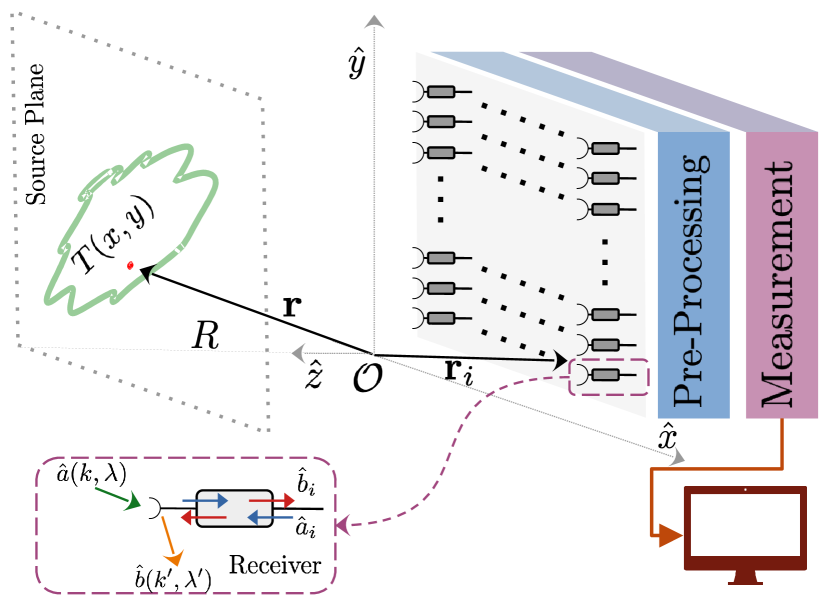
Figure 1: A interferometer, with $n$ receivers, separated by a distance $R$ from the source plane. The $T_{\mathrm{eff}}(x,y)$ is the position-dependent effective temperature in the source plane that one wants to measure. The field propagating from the source scatters each receiver on the interferometer. We consider the origin of the coordinate system on the detection plane as $\mathcal{O}$. All the components of the vectors are donated in the coordinate system $\mathcal{R}=(\mathcal{O},\hat{e}_{x},\hat{e}_{y},\hat{e}_{z})$.

This matrix acts on the vector $\left[\hat{a}(\mathbf{k},\sigma),\hat{a}_{i}\right]^{T}$. The first block, $\mathcal{S}^{(\text{scat })}$, describes the scattering of incoming plane waves to outgoing plane waves from the interferometer. A receiver can receive or transmit the signal. The off-diagonal block $\mathcal{S}^{(\mathrm{rec})}$ describes the coupling of the incoming plane waves $\hat{a}(\mathbf{k},\sigma)$ into the receiver modes $\hat{b}_{i}$, and $\mathcal{S}^{(\operatorname{trans})}$ describes scattering of reflected receiver modes $\hat{a}_{i}$ into outgoing plane waves $\hat{b}(\mathbf{k},\sigma)$. The matrix $\mathcal{S}^{(\text{refl })}$ represents the scattering (reflection) between the receivers, and will be neglected, $\mathcal{S}^{(\text{refl })}\sim 0$. One can also verify that if the receivers have only incoming and outgoing modes, the receiving and transmitting pattern of the receivers will be the same $\mathcal{S}^{(\operatorname{trans})}(\mathbf{k},\sigma;j)=\mathcal{S}^{(\operatorname{rec})}(j;\mathbf{k},\sigma)$ and we can denote them as simply $\mathcal{S}_{j}(\mathbf{k},\sigma)$. Formally, the input-output relations read

$$\begin{split}\hat{b}(\mathbf{k},\sigma)=&\sum_{\sigma^{\prime}}\int{d}^{3}\mathbf{k}^{\prime}\mathcal{S}^{(\mathrm{scat})}\left(\mathbf{k},\mathbf{k}^{\prime},\sigma,\sigma^{\prime}\right)\hat{a}\left(\mathbf{k}^{\prime},\sigma^{\prime}\right)\\ &+\sum_{j}\mathcal{S}_{j}(\mathbf{k},\sigma)\hat{a}_{j},\end{split}$$ (12)

and,

$$\hat{b}_{i}=\sum_{\sigma}\int\mathrm{d}^{3}\mathbf{k}\mathcal{S}_{i}\left(\mathbf{k},\sigma\right)\hat{a}\left(\mathbf{k},\sigma\right).$$ (13)

For a lossless system we can assume that $S^{\dagger}S=I$. Then we can write $\mathcal{S}^{(\mathrm{scat})}\left(\mathbf{k},\mathbf{k}^{\prime},\sigma,\sigma^{\prime}\right)=(\mathcal{S}^{(\mathrm{scat})})^{T}\left(\mathbf{k}^{\prime},\mathbf{k},\sigma^{\prime},\sigma\right)$. The field operators $\hat{a}(\mathbf{k},\sigma)$ from the state that we have for Eq. (7) can be replaced by the following relation for $n$ different receiver modes

$$\begin{split}\hat{a}(\mathbf{k},\sigma)&=\sum_{j}^{n}{\mathcal{S}^{*}_{j}(\mathbf{k},\sigma)}\hat{b}_{j}\\ &+\sum_{\sigma^{\prime}}\int d^{3}\mathbf{k^{\prime}}{\mathcal{S}^{*(\mathrm{scat})}(\mathbf{k}^{\prime},\sigma^{\prime},\mathbf{k},\sigma)}\hat{b}(\mathbf{k}^{\prime},\sigma^{\prime}).\end{split}$$ (14)

The interferometer does not have any access to modes $\hat{b}(\mathbf{k},\sigma)$. For an array of receivers at positions $\mathbf{r}_{i}$ in the detection plane, each scattering function may be written as [59]

$$\begin{split}\mathcal{S}_{i}(\mathbf{k},\sigma)=e^{i\mathbf{k}\cdot\mathbf{r}_{i}-\omega t_{i}}\mathcal{S}(\mathbf{k},\sigma),\end{split}$$ (15)

where $t_{i}$ is the time at which we consider the state of the $i$-th receiver. We can assume that for all receivers $t_{i}\equiv\bar{t}>t-|\mathbf{r}-\mathbf{r}_{i}|/c$ due to retardation, where according to (14), $t$ is the last time the current densities to be sensed imprint their information the coherent state labels $\alpha(\bm{k},\sigma)$. And $\mathcal{S}(\mathbf{k},\sigma)$ is the function describes scattering to the central receiver. Further, the commutation relation of different receiver modes can be written as

$$[\hat{b}_{i},\hat{b}_{j}^{\dagger}]=\sum_{\sigma}\int\mathrm{d}^{3}\mathbf{k}\mathcal{S}_{i}\left(\mathbf{k},\sigma\right)\mathcal{S}_{j}^{*}\left(\mathbf{k},\sigma\right)\approx\delta_{ij}.$$ (16)

where we have used the canonic commutation relation of $\hat{a}\left(\mathbf{k},\sigma\right)$ and we assumed that $|\mathcal{S}(\mathbf{k},\sigma)|$ varies slowly compared to the oscillations of the exponential factor $\exp(i\mathbf{k}\cdot(\mathbf{r}_{i}-\mathbf{r}_{j}))$ for $i\neq j$. Since $\hat{b}_{i}$ commutes with $\hat{b}(\mathbf{k},\sigma)$, using Eq. (14) we can write the coherent state in Eq. (7) as

$$\begin{split}\ket{\psi(t)}=D(\{\beta_{i}\})D(\{\beta(\mathbf{k},\sigma)\})\ket{\{0\}}.\end{split}$$ (17)

After, tracing out the modes $\hat{b}(\mathbf{k},\sigma)$ we have a coherent state

$$\begin{split}\rho^{\prime}=\ket{\{\beta_{i}\}}\bra{\{\beta_{i}\}},\end{split}$$ (18)

and the displacement operator can be written in the form

$$\begin{split}D(\{\beta_{i}\})=\bigotimes_{i}^{n}\mathrm{exp}\left[\beta_{i}\hat{b}_{i}^{\dagger}-\beta_{i}^{*}\hat{b}_{i}\right]\end{split}$$ (19)

where

$$\begin{split}\beta_{i}&=\sum_{\sigma}\int d^{3}{k}\;S_{i}(\mathbf{k},\sigma)\alpha(\mathbf{k},\sigma)\,.\end{split}$$ (20)

$\mathcal{S}_{i}(\mathbf{k},\sigma)$ depends on the type of receivers. Let us assume that each receiver is characterized by a filter function $w(\omega)$ with central frequency $\omega_{0}$ and bandwidth $B\ll\omega_{0}$,

$$w(\omega)=\left\{\begin{array}[]{ll}1&\text{ for }\omega_{0}-B/2\leqslant\omega\leqslant\omega_{0}+B/2\\ 0&\text{ elsewhere }\end{array}\right..$$ (21)

For simplicity we assume $S(\mathbf{k},\sigma)\propto\sqrt{\omega}w(\omega)\bm{\varepsilon}(\mathbf{k},\sigma)\cdot\hat{u}$, and normalized according to Eq. (16) as

$$S(\mathbf{k},\sigma)=\left(\frac{3c^{3}\omega}{8\pi\omega_{0}^{3}B}\right)^{1/2}w(\omega)\bm{\varepsilon}(\mathbf{k},\sigma)\cdot\hat{u}$$ (22)

where $\omega=c|\mathbf{k}|$ and $\hat{u}$ is the unit polarization direction of the corresponding receiver mode. Then we have

$$\begin{split}\beta_{i}=&{-\left(\frac{3c^{3}}{2^{8}\hbar\varepsilon_{0}\pi^{5}\omega_{0}^{3}B}\right)^{1/2}}\int d^{3}{r}\;\int_{-\infty}^{\infty}d\tilde{\omega}\\ &\times\sum_{\sigma}\int d^{3}{k}\;{w(\omega)}\tilde{\mathbf{j}}\left(\mathbf{r},\tilde{\omega}\right)\cdot\bm{\varepsilon}(\mathbf{k},\sigma)\bm{\varepsilon}(\mathbf{k},\sigma)\cdot\hat{u}\\ &\times\frac{e^{i(\tilde{\omega}t+\omega t-\omega\bar{t})}e^{-i\mathbf{k}\cdot(\mathbf{r}-\mathbf{r}_{i})}}{i\epsilon-c|\mathbf{k}|-\tilde{\omega}}.\end{split}$$ (23)

To take the integral over $d^{3}{k}$ we align the $k_{z}$-axis with the vector $\left(\mathbf{r}-\mathbf{r}_{i}\right)$. In spherical coordinates in $k$-space we have $d^{3}{k}=\omega^{2}/c^{3}d\omega d\Omega$, where $\omega=|\mathbf{k}|c$ and $\mathbf{k}=(\omega/c)\hat{\mathbf{n}}(\Omega)$ with $\hat{\mathbf{n}}(\Omega)=(\sin\theta\cos\phi,\sin\theta\sin\phi,\cos\theta)$. The two polarizations can be written in the form $\bm{\varepsilon}(\Omega,1)=(\sin\phi,-\cos\phi,0)$ and $\bm{\varepsilon}(\Omega,2)=(\cos\theta\cos\phi,\cos\theta\sin\phi,-\sin\theta)$. Taking the integral over $\Omega$, summing over two polarizations, and using one of the approximations of the far field limit $\omega|\mathbf{r}-\mathbf{r}_{i}|/c\gg 1$, gives

$$\begin{split}\beta_{i}=&{i}\left(\frac{3c\mu_{0}}{64\hbar\pi^{3}\omega_{0}^{3}B}\right)^{1/2}\int d^{3}{r}\int_{-\infty}^{\infty}d\tilde{\omega}\int_{0}^{\infty}d\omega{w(\omega)}{\omega}\\ &\times\tilde{\mathbf{j}}_{t}\left(\mathbf{r},\tilde{\omega}\right)\cdot\hat{u}\frac{e^{i\omega|\mathbf{r}-\mathbf{r}_{i}|/c}-e^{-i\omega|\mathbf{r}-\mathbf{r}_{i}|/c}}{|\mathbf{r}-\mathbf{r}_{i}|}\frac{e^{i(\tilde{\omega}t+\omega t-\omega\bar{t})}}{i\epsilon-\omega-\tilde{\omega}},\end{split}$$ (24)

where $\tilde{\mathbf{j}}_{t}\left(\mathbf{r},\tilde{\omega}\right)$ is the locally transverse component of the current density defined as $\tilde{\mathbf{j}}_{t}=\tilde{\mathbf{j}}-(\tilde{\mathbf{j}}\cdot\hat{e}_{\mathbf{r}})\hat{e}_{\mathbf{r}}$ with unit vector $\hat{e}_{\mathbf{r}}=(\mathbf{r}-\mathbf{r}_{i})/|\mathbf{r}-\mathbf{r}_{i}|.$ Since $R\gg|\mathbf{r}_{i}|$, we have $\hat{e}_{\mathbf{r}}\approx\mathbf{r}/|\mathbf{r}|$, with corrections modifying only slightly the prefactors, not the phases. One can extend the lower bound of the integration range of the ${\omega}$ integral to $-\infty$ using the definition of $w(\omega)$, and evaluate the $\omega$ integral with the help of the law of residues. Since $-\bar{t}+t-|\mathbf{r}-\mathbf{r}_{i}|/c<0$, the pole at $\omega=-\tilde{\omega}+i\epsilon$ contributes to the term $\exp{(i\omega|\mathbf{r}-\mathbf{r}_{i}|/c)}$. For $\exp{(-i\omega|\mathbf{r}-\mathbf{r}_{i}|/c)}$ the contour must be closed in the lower half plane and there is no pole to contribute. In the end one should send $\epsilon\rightarrow 0$. Then $\beta_{i}$ simplifies to

$$\begin{split}\beta_{i}=&-\left(\frac{3c\mu_{0}}{16\pi\hbar\omega_{0}^{3}B}\right)^{1/2}\int_{-\infty}^{\infty}d\omega{w(-\omega)}{\omega}\int d^{3}{r}\\ &\times\tilde{\mathbf{j}}_{t}\left(\mathbf{r},{\omega}\right)\cdot\hat{u}\frac{e^{-i\omega(\bar{t}-|\mathbf{r}-\mathbf{r}_{i}|/c})}{|\mathbf{r}-\mathbf{r}_{i}|}.\end{split}$$ (25)

where we drop the "$\sim$" from $\tilde{\omega}$. The state in Eq. (7) is written for a deterministic current density distribution. In reality, these current densities fluctuate. Before we move forward, we describe the properties of these current density distribution. We assume that it is a complex symmetric Gaussian process with current densities uncorrelated in positions, directions and frequencies [43, 61, 62],

$$\small\begin{split}&\left\langle\tilde{j}_{i}\left(\mathbf{r},\omega\right)\tilde{j}_{j}^{*}\left(\mathbf{r}^{\prime},\omega^{\prime}\right)\right\rangle=\frac{l_{c}^{3}}{\tau_{c}}\delta_{ij}\delta(\omega-\omega^{\prime})\delta(\mathbf{r}-\mathbf{r}^{\prime})\braket{}{\tilde{{j}}_{i}(\mathbf{r},\omega)}{{}^{2}},\\ &\left\langle\tilde{j}_{i}\left(\mathbf{r},\omega\right)\tilde{j}_{j}\left(\mathbf{r}^{\prime},\omega^{\prime}\right)\right\rangle=0,\quad\left\langle\tilde{j}^{*}_{i}\left(\mathbf{r},\omega\right)\tilde{j}_{j}^{*}\left(\mathbf{r}^{\prime},\omega^{\prime}\right)\right\rangle=0\,.\end{split}$$ (26)

The length scale $l_{c}$ and time scale $\tau_{c}$ are introduced for dimensional grounds. We choose the unit polarization vector of the receiver $\hat{u}$ as one of basis vectors of the coordinate system $\mathcal{R}$ parallel to the detection plane, $\hat{u}=\hat{e}_{i}$ where $i\in\{x,y\}$. Then, we can write $\langle{\tilde{\mathbf{j}}_{t}(\mathbf{r},\omega)\cdot\hat{u}\tilde{\mathbf{j}}^{*}_{t}(\mathbf{r},\omega)\cdot\hat{u}}\rangle=\langle{|\tilde{{j}}_{t,i}(\mathbf{r},\omega)|^{2}}\rangle$. Using Eq. (18) and introducing the distribution of the current density $P({\tilde{j}}({r},\omega))$, the state for the interferometer $\rho_{\mathrm{int}}$ with $n$ receivers can be written as

$$\rho_{\mathrm{int}}=\int d^{2}{\tilde{j}}P({\tilde{j}}(\mathbf{r},\omega))|\{\beta_{i}\}\rangle\langle\{\beta_{i}\}|.$$ (27)

The integral is over the complex ${\tilde{j}}$ plane. Gaussian states are completely characterized by their mean displacement $\Gamma_{i}=\operatorname{Tr}\left[\rho\mathbf{b}_{i}\right]$ and covariance matrix with elements $\Sigma_{ij}=\frac{1}{2}\operatorname{Tr}\left[\rho\left(\tilde{\mathbf{b}}_{i}\tilde{\mathbf{b}}_{j}+\tilde{\mathbf{b}}_{j}\tilde{\mathbf{b}}_{i}\right)\right],$ where $\mathbf{b}=\left[b_{1},b_{1}^{\dagger},b_{2},b_{2}^{\dagger},...b_{n},b_{n}^{\dagger}\right]$ and $\quad\tilde{\mathbf{b}}_{i}=\mathbf{b}_{i}-\Gamma_{i}$  [63, 64, 65, 66, 26, 67]. The mean displacement for our state is zero $\Gamma_{i}=0$ considering Eq. (26). To find the elements of the covariance matrix, we need to calculate $\braket{b^{\dagger}_{i}b_{j}}$. The integral over $\omega$ can be taken using the filter function of bandwidth $B$. With this we find

$$\begin{split}\braket{b^{\dagger}_{i}b_{j}}&=K\int d^{3}{r}\;\frac{\braket{}{\tilde{{j}}_{t,i}\left(\mathbf{r},{\omega}\right)}{{}^{2}}e^{i\omega_{0}(|\mathbf{r}-\mathbf{r}_{j}|-|\mathbf{r}-\mathbf{r}_{i}|)/c}}{|\mathbf{r}-\mathbf{r}_{i}||\mathbf{r}-\mathbf{r}_{j}|}\\ &\times\mathrm{sinc}\left[\frac{B}{2c}(|\mathbf{r}-\mathbf{r}_{j}|-|\mathbf{r}-\mathbf{r}_{i}|)\right]\end{split}$$ (28)

where, $K=3c\mu_{0}l_{c}^{3}/(16\pi\hbar\omega_{0}\tau_{c})$ and $\mathrm{sinc}[x]\equiv\sin x/x$. For a very narrow bandwidth $\mathrm{sinc}[...]\approx 1$. Then Eq. (28) for $i=j$ becomes

$$\begin{split}\bar{n}&=K\int d^{3}{r}\;\frac{\braket{}{\tilde{{j}}_{t,i}\left(\mathbf{r},{\omega}\right)}{{}^{2}}}{|\mathbf{r}-\mathbf{r}_{i}|^{2}}\,.\end{split}$$ (29)

where we defined $\bar{n}\equiv\braket{b^{\dagger}_{i}b_{i}}$ without any index, since the mean photon number is the same for all interferometer modes in the far-field approximation, and for $i\neq j$ it becomes

$$\begin{split}\xi_{ij}&=K\int d^{3}{r}\;\frac{\braket{}{\tilde{{j}}_{t,i}\left(\mathbf{r},{\omega}\right)}{{}^{2}}e^{i\omega_{0}(|\mathbf{r}-\mathbf{r}_{j}|-|\mathbf{r}-\mathbf{r}_{i}|)/c}}{|\mathbf{r}-\mathbf{r}_{i}||\mathbf{r}-\mathbf{r}_{j}|}\,.\end{split}$$ (30)

with $\xi_{ij}\equiv\braket{b^{\dagger}_{i}b_{j}}$. The integral over Earth’s surface is parametrized by $\mathbf{r}=(x,y,R)$ with respect to the coordinate system of the detection plane. Further, we write $|\mathbf{r}-\mathbf{r}_{j}|-|\mathbf{r}-\mathbf{r}_{i}|\approx\Delta\mathbf{r}_{ij}\cdot\mathbf{r}/|\mathbf{r|}$ for $|\Delta\mathbf{r}_{ij}|\ll R$, where $\Delta\mathbf{r}_{ij}=\mathbf{r}_{j}-\mathbf{r}_{i}$ connects two different receiver modes. In the denominator, we approximate $|\mathbf{r}-\mathbf{r}_{i}|\approx R/\cos\tilde{\theta}(x,y)$ with $\tilde{\theta}(x,y)$ the polar angle the angle between the $z$-axis and the vector $(x,y,R)$. One can relate the average amplitude of current density to brightness temperature $T_{\mathrm{B}}(x,y)$ by $\braket{}{\tilde{{j}}_{t,i}\left(\mathbf{r},{\omega}\right)}{{}^{2}}=K_{1}T_{\mathrm{B}}(x,y)\cos\tilde{\theta}(x,y)\delta(z-R)$ with a constant defined as $K_{1}=32\tau_{c}k_{B}/(3l_{c}^{3}\mu_{0}c)$ (See Appendix A). We define the effective temperature as $T_{\mathrm{eff}}(x,y)\equiv T_{\mathrm{B}}(x,y)\cos^{3}\tilde{\theta}(x,y)$ and a new constant $\kappa=K_{1}K\equiv{2k_{B}}/{(\pi\hbar\omega_{0})}$ where $\kappa$ has the dimension of inverse temperature with SI-units "$[1/\mathrm{K}]$". Then we can simplify Eq. (29) for $i=j$ as

$$\begin{split}\bar{n}&=\frac{\kappa}{R^{2}}\int dxdy\;T_{\mathrm{eff}}(x,y),\end{split}$$ (31)

and for $i\neq j$ as

$$\begin{split}\xi_{ij}&=\frac{\kappa}{R^{2}}\int dxdy\;T_{\mathrm{eff}}(x,y)e^{2\pi i\left(v_{x}^{ij}x+v_{y}^{ij}y\right)},\end{split}$$ (32)

where

$$\begin{split}v_{y}^{ij}=\frac{\Delta x_{ij}}{\lambda R},\qquad v_{x}^{ij}=\frac{\Delta y_{ij}}{\lambda R}.\end{split}$$ (33)

We used $\omega_{0}/c=2\pi/\lambda$. These two equations suffice to determine the covariance matrix elements of the Gaussian states for the general interferometer with an array of receivers. All spatial field modes received by the interferometer undergo a preprocessing before measurement. This processing can be understood as a linear combination of all spatial modes in such a way to achieve the optimal POVM for the best estimation of the parameter we are interested in. See section II.3. We use the values of the SMOS for the rest of the paper which leads to $\kappa\sim 9.4\>[1/\mathrm{K}]$.

II.3 Quantum Cramér-Rao Bound

A lower bound of an unbiased estimator of a deterministic parameter is given by the Cramér-Rao (CR) bound, which states that the variance of any such estimator is equal or greater than the inverse of the Fisher information. The quantum analog of the Cramér-Rao bound is the quantum Cramér-Rao bound (QCRB), given by the inverse of the quantum Fisher information (QFI). The significance of the QCRB lies in the fact that in the case of a single parameter to be estimated the bound can in principle be saturated in the limit of infinitely many measurements when chosing the optimal quantum measurement and maximum-likelihood estimation. Let us consider a quantum state $\rho_{\bm{\mu}}$ that depends on a vector of $l$ parameters, $\bm{\mu}=(\mu_{1},\mu_{2},...,\mu_{l})^{T}$. One can generalize the single-parameter quantum Cramér-Rao bound (QCRB)  [5, 4] to the multiparameter QCRB  [68] given for a single measurement by

$$\operatorname{Cov}(\tilde{\bm{\mu}})\geqslant\mathscr{F}(\bm{\mu})^{-1},\quad\mathscr{F}_{{ij}}(\bm{\mu})=\frac{1}{2}\operatorname{tr}\left(\rho_{\bm{\mu}}\left\{\mathscr{L}_{i},\mathscr{L}_{j}\right\}\right),$$ (34)

where $\operatorname{Cov}(\tilde{\bm{\mu}})$ is a covariance matrix for the locally unbiased estimator $\tilde{\bm{\mu}}(x)$ [53, 48], the $\{\cdot,\cdot\}$ means the anti-commutator, and $\mathscr{L}_{i}$ is the symmetric logarithmic derivative (SLD) related to parameter $i$, which is defined similarly to the single-parameter case, $\frac{1}{2}\left(\mathscr{L}_{i}\rho_{\bm{\mu}}+\rho_{\bm{\mu}}\mathscr{L}_{i}\right)=\partial_{{i}}\rho_{\bm{\mu}}.$ Contrary to the single parameter case, the multiparameter QCRB can in general not be saturated, but gives a useful lower bound nevertheless.

The SLD and the elements of QFI matrix are given in Ref. [65] for any Gaussian state. The SLD can be written as

$$\mathscr{L}_{i}=\frac{1}{2}\mathfrak{M}_{\alpha\beta,\gamma\delta}^{-1}\left(\partial_{i}\Sigma^{\gamma\delta}\right)\left(\mathbf{b}_{\alpha}\mathbf{b}_{\beta}-\Sigma^{\alpha\beta}\right),$$ (35)

where the summation convention is used. In our case, the mean displacement of Gaussian state is zero. Thus, we can simplify further the elements of the QFI matrix in [65] to

$$\mathscr{F}_{ij}=\frac{1}{2}\mathfrak{M}_{\alpha\beta,\gamma\delta}^{-1}\partial_{j}\Sigma^{\alpha\beta}\partial_{i}\Sigma^{\gamma\delta},$$ (36)

where

$$\mathfrak{M}\equiv\Sigma\otimes\Sigma+\frac{1}{4}\Omega\otimes\Omega,$$ (37)

and $\Omega=\bigoplus_{k=1}^{n}i\sigma_{y}$. Using the properties of the Gaussian state (circularly symmetric and with zero mean) we can write the SLD for $n$ mode interferometers as

$$\begin{split}\mathscr{L}_{i}=\sum_{j}^{n}g^{j}_{i}\hat{b}^{\dagger}_{j}\hat{b}_{j}+\sum_{j<k}^{n}(g^{jk}_{i}\hat{b}^{\dagger}_{j}\hat{b}_{k}+(g^{jk}_{i})^{*}\hat{b}^{\dagger}_{k}\hat{b}_{j})+\mathrm{C},\end{split}$$ (38)

where C is a constant term. In the single parameter case, the optimal POVM is the set of projectors onto eigenstates of $\mathscr{L}_{i}$. It allows one to saturate the QCRB in the limit of infinitely many measurements and maximum likelihood estimation [4, 69, 70]. In the multiparameter case, (34) can in general not be saturated. For the diagonalization of the SLD, the constant C is not important and we can drop it from the beginning. We construct a Hermitian matrix $\mathbf{M}_{i}$

$$\mathbf{M}_{i}=\left[\begin{array}[]{cccc}g^{1}_{i}&g^{12}_{i}&...&g^{1n}_{i}\\ (g^{12}_{i})^{*}&g^{2}_{i}&...&g^{2n}_{i}\\ ...&...&...&...\\ (g^{1n}_{i})^{*}&(g^{2n}_{i})^{*}&...&g^{n}_{i}\end{array}\right],$$ (39)

where the diagonal elements are real-valued functions which can be defined as $g^{j}_{i}=\mathfrak{M}_{\alpha\beta,\gamma\delta}^{-1}\left(\partial_{i}\Sigma^{\gamma\delta}\right)$ with $\alpha=2j$ and $\beta=2j-1$. The off-diagonal elements are complex-valued functions which are defined as $g^{jk}_{i}=\mathfrak{M}_{\alpha\beta,\gamma\delta}^{-1}\left(\partial_{i}\Sigma^{\gamma\delta}\right)$ with $\alpha=2j$ and $\beta=2k-1$ and $k>j$. Further, we can define a new set of operators $\bar{\mathbf{b}}^{\dagger}\equiv{\left[\hat{b}_{1}^{\dagger},\hat{b}_{2}^{\dagger},...,\hat{b}_{n}^{\dagger}\right]}$ and $\bar{\mathbf{b}}\equiv{\left[\hat{b}_{1},\hat{b}_{2},...,\hat{b}_{n}\right]^{T}}$. Then the SLD becomes

$$\begin{split}\mathscr{L}_{i}=\bar{\mathbf{b}}^{\dagger}\mathbf{M}_{i}\bar{\mathbf{b}}.\end{split}$$ (40)

Since $\mathbf{M}_{i}$ is a Hermitian matrix, it can always be unitarily diagonalized by $\mathbf{M}_{i}=\mathbf{V}^{\dagger}_{i}\mathbf{D}_{i}\mathbf{V}_{i}$ with $\mathbf{V}_{i}^{\dagger}\mathbf{V}_{i}=I$. A new set of operators can be defined as $\bar{\mathbf{d}}_{i}^{\dagger}=\bar{\mathbf{b}}^{\dagger}\mathbf{V}_{i}^{\dagger}$ where $\bar{\mathbf{d}}_{i}^{\dagger}={\left[\hat{d}_{i1}^{\dagger},\hat{d}_{i2}^{\dagger},...,\hat{d}_{in}^{\dagger}\right]}$. The optimal POVM for the single parameter case ($i=1$, which we drop in the following) can be found as a set of projectors in the Fock basis $\{\ket{m_{1},m_{2},...,m_{n}}\bra{m_{1},m_{2},...,m_{n}}\}_{\{m_{1},m_{2}...m_{n}\}}$ of the $\hat{d}_{l}$ with $\hat{d}^{\dagger}_{l}\hat{d}_{l}\ket{m_{1},m_{2},...,m_{n}}=m_{l}\ket{m_{1},m_{2},...,m_{n}}$, where $l\in\{1,...,n\}$. The $\hat{d}_{l}$ will be called "detection modes".

III Results

III.1 The Single Receiver

In this section, we consider the case of the simplest estimation of the parameters of the sources with a single receiver with mode $\hat{b}$. Then the covariance matrix for the state can be written as

$$\Sigma =\left[\begin{array}[]{cccc}0&\chi\\ \chi&0\end{array}\right].$$ (41)

The QFI matrix elements for single mode can be found as

$$\begin{split}\mathscr{F}_{ij}=\frac{4\partial_{i}\chi\partial_{j}\chi}{4\chi^{2}-1},\end{split}$$ (42)

and, up to the irrelavant constant, the SLD becomes,

$$\begin{split}\mathscr{L}_{i}=\frac{4\partial_{i}\chi}{4\chi^{2}-1}\hat{b}^{\dagger}b.\end{split}$$ (43)

Since the SLD is already diagonal in the basis of $\hat{b}^{\dagger}\hat{b}$, the detection mode can be considered as $\hat{b}$. We write the POVM obtained from the SLD as a set of projectors in the Fock basis $\{\ket{m}\bra{m}\}_{\{m\}}$ which is the eigenbasis of $\hat{b}^{\dagger}\hat{b}$, $\hat{b}^{\dagger}\hat{b}\ket{m}\bra{m}=m\ket{m}\bra{m}$. To compare, we consider the POVM from heterodyne detection. The heterodyne detection uses a classical local oscillator to make a measurement locally on the basis of coherent states. For a single mode, its POVM elements can be written as $E(\nu)=\ket{\nu}\bra{\nu}/\pi$ where $\ket{\nu}$ is coherent state and $\int d^{2}\nu E(\nu)=\mathds{1}$. The probability that $E(\nu)$ triggers reads

$$\begin{split}P(\nu|\mu_{i})=\frac{1}{\pi(1+\bar{n})}\exp\left[-\frac{|\nu|^{2}}{(1+\bar{n})}\right]\,,\end{split}$$ (44)

with $\bar{n}$ given by eq.(31). The classical Fisher information (CFI) for parameter $\mu_{i}$ can be written as

$$\begin{split}F_{i}&=\int d^{2}\nu\frac{1}{P(\nu|\mu_{i})}\left(\frac{\partial P(\nu|\mu_{i})}{\partial\mu_{i}}\right)^{2}.\end{split}$$ (45)

The Resolution of a Uniform Circular Source: Consider a source defined as a circular disk with radius $a$ and with uniform temperature $T$ located under the interferometer at a distance $R$, ($\mathbf{r}=(0,0,R)$). We assume $a\ll R$. Then only small angles are involved and one can set $\cos^{3}\Theta(x,y)\approx 1$. This corresponds to one of the approximations characteristic of the far field regime [71].

$$T_{\mathrm{eff}}(x,y)=T\operatorname{circ}(x,y),$$ (46)

where the symbol $\mathrm{circ}(\cdot)$ stands for the circular function, defined as

$$\operatorname{circ}(x,y)\triangleq\left\{\begin{array}[]{ll}1&\sqrt{x^{2}+y^{2}}\leq a\\ 0&\sqrt{x^{2}+y^{2}}>a\end{array}\right.$$ (47)

$$\begin{split}\bar{n}&=\frac{\kappa T}{R^{2}}\int dxdy\operatorname{circ}(x,y)\\ &=\frac{\pi a^{2}\kappa T}{R^{2}},\end{split}$$ (48)

and $\chi$ becomes $\chi={1}/{2}+\bar{n}$. We may consider $a$ and $T$ as the parameter that we want to estimate. The QFI for estimating $a$ becomes

$$\begin{split}\mathscr{F}_{a}=\frac{4\pi T\kappa}{R^{2}+a^{2}\pi T\kappa}.\end{split}$$ (49)

Then we can write the SLD for estimating the $a$ ignoring the constant term as

$$\begin{split}\mathscr{L}_{a}=\frac{2R^{2}}{aR^{2}+a^{3}\pi T\kappa}\hat{b}^{\dagger}\hat{b}.\end{split}$$ (50)

The optimal POVM is a set of projectors in the Fock basis $\{\ket{m}\bra{m}\}_{\{m\}}$. The CFI of the heterodyne detection becomes

$$\begin{split}{F}_{a}=\frac{4a^{2}\pi^{2}T^{2}\kappa^{2}}{(R^{2}+a^{2}\pi T\kappa)^{2}}.\end{split}$$ (51)

In Fig. (2), we compare the QFI with the CFI of heterodyne detection. As one can see, for small source sizes, the Fisher information from heterodyne measurement vanishes. However, the QFI tends to a constant. For instance, in the limit $a\rightarrow 0$, for $T=300$ [K] we have QFI for estimating $a$ as $\mathscr{F}_{a}\sim 6.16\times 10^{-2}\;\mathrm{[1/km^{2}]}$, which gives a smallest standard deviation of about $4$ [km]. Thus, we can conclude that the photon number measurement on the complete basis of Fock states in the detection mode $\hat{b}$ helps us to get better resolution than heterodyne measurement. If $a$ becomes larger, we can see that the QFI and CFI get close to each other at some point. To estimate $a$, we assumed that we know exactly the temperature of the source. Fig. (2b) shows that QFI for estimating the temperature tends to zero in the limit $a\rightarrow 0$. This demonstrates that one can not determine the temperature of infinitely small sources with this method.

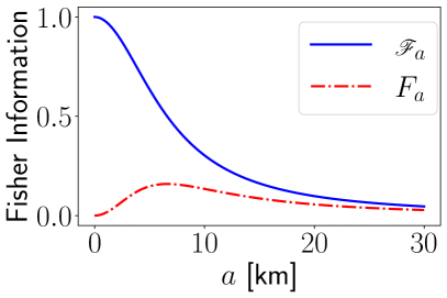
(a)

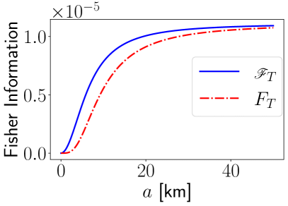
(b)

Figure 2: a) The Fisher information (dimensionless) concerning source size. The solid blue line shows the QFI for estimating the source size. The red dashed line shows the CFI that one gets from the heterodyne measurement. Both results are scaled with the $4\pi T\kappa/R^{2}$, considering $T=300$ [K]. b) The Fisher information concerning the temperature. The solid blue line shows the QFI for estimating the temperature. The red dashed line shows the CFI that one gets from the heterodyne measurement. Both results are in units of [$\mathrm{1/K^{2}}$], and we consider $T=300$ [K].

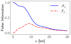
(a)

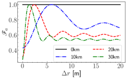
(b)

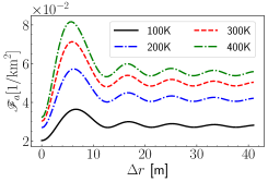
(c)

Figure 3: a) The Fisher information concerning source size. The solid blue line shows the QFI for estimating the source size. The red dashed line shows the CFI from the heterodyne measurement. Both of the results are scaled with the Eq. (61). In the limit $a\rightarrow 0$, for $T=300$ [K], we have $\mathscr{F}_{a}\sim 0.117\;[1/\mathrm{km}^{2}]$, which gives us a standard deviation around $2.92$ [km]. b) The QFI $\mathscr{F}_{a}$ for estimating the size of the circular disc as a function of $\Delta r$ (spatial separation of two receivers) for different source sizes $a$ with $T=300$ [K]. Each data scaled by the maximum value of the QFI for $a=(0,10,20,30)$ [km], which are $(\sim 0.117,\sim 0.070,\sim 0.030,\sim 0.015)[1/\mathrm{km}^{2}]$, respectively. c) The QFI $\mathscr{F}_{a}$ for estimating the size of the circular disc as a function of separation of two receivers $\Delta r$, for different temperatures $T$.)

Further, we can find the QFI for estimating the temperature as

$$\begin{split}\mathscr{F}_{T}=\frac{\pi a^{2}\kappa}{R^{2}T+a^{2}\pi T^{2}\kappa},\end{split}$$ (52)

with a SLD given by

$$\begin{split}\mathscr{L}_{T}=\frac{R^{2}}{TR^{2}+a^{2}\pi T^{2}\kappa}\hat{b}^{\dagger}\hat{b}.\end{split}$$ (53)

The CFI from heterodyne detection to estimate temperature becomes

$$\begin{split}{F}_{T}=\frac{\pi^{2}a^{4}\kappa^{2}}{(R^{2}+a^{2}\pi T\kappa)^{2}}.\end{split}$$ (54)

In Fig.(2b), we plot both QFI and CFI for heterodyne detection for temperature estimation. Both have very close functional behavior. They vanish for $a\rightarrow 0$ and they approach each other when we have a large source size.

The off-diagonal matrix element of the QFI matrix for multiparameter estimation reads

$$\begin{split}\mathscr{F}_{aT}=\frac{2a\pi\kappa}{R^{2}+a^{2}\pi T\kappa}.\end{split}$$ (55)

By sampling the same state $\mathcal{N}$ times, the standard deviation of the estimator decreases proportional to $1/\sqrt{\mathcal{N}}$. The SMOS satellite moves at a constant speed $v\simeq 7$ [km/s] and takes the time $\tau=L/v$ to fly over a distance $L$. For each sample there is a lower bound for the detection time given by $t_{D}\sim 1/B$ (see appendix A). In practice, the effective detection time might be much larger, due to, e.g. deadtimes of the detectors, slow electronics, etc. In addition, zero temperature of the detector and modes $b_{i}$ is implicitly assumed in our calculations, but would require cooling down to temperatures much smaller than $\hbar\omega_{0}$. If the actual detection time is $t_{D}^{\text{eff}}$, the sample size becomes $\mathcal{N}=\tau/t_{D}^{\text{eff}}$. In this paper we intend to establish the ultimate theoretical bounds and hence assume that the minimal detection time $t_{D}=1/B$ can be achieved, in which case the sample size becomes $\mathcal{N}\sim LB/v$. To estimate the source size one can assume that $L\sim a$, and the QCRB for estimating $a$ becomes $\delta a\geq 1/\sqrt{\mathcal{N}\mathcal{F}_{a}}$. Since $\mathcal{N}$ depends also on $a$ one can find the optimum bound in the sense of a minimal $\delta a$ at $a=R/\sqrt{\pi\kappa T}$. For $T=300$ [K], we find $a\sim 7.9$ [km] and $\delta a\gtrsim 1.0$ [m]. The bound for estimating $T$, assuming all other parameters known, can be written as $\delta T\geq 1/\sqrt{\mathcal{N}\mathcal{F}_{T}}$. Using the same parameters as before and the same sample size, we have $\delta T\gtrsim 0.08$ [K]. Thus, increasing the sample size to the theoretically maximally possible value, the spatial resolution improves by a factor of order 35,000 compared to the resolution of SMOS, and the radiometric resolution by factor of order 500. One can also increase the resolution by increasing the number of receivers, which we present in the following sections.

III.2 Two Mode Interferometer

In the previous section, we only considered a single receiver with mode $\hat{b}$. It is obvious that we may get additional information from the cross correlations of an $n$ mode interferometer. An analytical calculation of the QFI matrix for $n$ mode interferometer generally becomes untractable for $n>2$ and one has to rely on numerical calculation, see Section III.3. Here, we consider the next simplest case of two receivers with modes $\hat{b}_{1}$ and $\hat{b}_{2}$. Then we can write $\mathbf{b}$ as $\mathbf{b}^{\top}=(\hat{b}_{1},\hat{b}_{1}^{\dagger},\hat{b}_{2},\hat{b}_{2}^{\dagger})$. The mean displacement is $\Gamma_{i}=0$. The covariance matrix $\Sigma$ of the state $\rho_{\mathrm{int}}$ becomes

$$\Sigma =\left[\begin{array}[]{cccc}0&\chi&0&\xi\\ \chi&0&\xi^{*}&0\\ 0&\xi^{*}&0&\chi\\ \xi&0&\chi&0\end{array}\right],$$ (56)

where $\chi=1/2+\bar{n}$ and $\xi=\braket{b_{2}^{\dagger}b_{1}}$. We give the general result for the QFI elements in Appendix B. Further one can write the matrix $\mathbf{M}$ as

$$\mathbf{M}_{i}=\left[\begin{array}[]{cccc}g^{1}_{i}&|g^{2}_{i}|e^{i\delta}\\ |g^{2}_{i}|e^{-i\delta}&g^{1}_{i}\end{array}\right],$$ (57)

where $g^{1}_{i},g^{2}_{i}$ are given in Appendix B in terms of $\chi$ and $\xi$, and $\delta$ is the phase difference between two modes in the SLD. Using the eigenvectors of $\mathbf{M}$ we can write the unitary $\mathbf{V}$ as

$$\mathbf{V}=\frac{1}{\sqrt{2}}\left[\begin{array}[]{cccc}1&e^{i\delta}\\ 1&-e^{i\delta}\end{array}\right],$$ (58)

We see that $\mathbf{V}$ does not depend on the magnitude of the elements of the matrix $\mathbf{M}$ for a two-mode interferometer. The detection modes can be found as $\hat{d}_{1}=(\hat{b}_{1}+\hat{b}_{2}e^{i\delta})/\sqrt{2}$ and $\hat{d}_{1}=(\hat{b}_{1}-\hat{b}_{2}e^{i\delta})/\sqrt{2}$. The preprocessing to combine these two modes can be done by a phase delay on one mode and then combining these two modes by a beam splitter before any measurement. Then the POVM for the optimum measurement can be written as a set of projectors again in Fock basis as $\{\ket{m_{1},m_{2}}\bra{m_{1},m_{2}}\}_{\{m_{1},m_{2}\}}$ which is the eigenbasis of $\hat{d}^{\dagger}_{i}\hat{d}_{i}$, $\hat{d}^{\dagger}_{i}\hat{d}_{i}\ket{m_{1},m_{2}}=m_{i}\ket{m_{1},m_{2}}$. To compare this POVM with the classical approach, we consider heterodyne detection in Appendix C.

Resolution of Uniform Circular Source: Let us assume that on the source plane, we have a circular disk of radius $a$ with uniform temperature $T$ located at $\mathbf{r}=(x_{0},y_{0},R)$. Then the temperature distribution over the surface on the source plane can be written as

$$T_{\mathrm{eff}}(x,y)=T\mathrm{circ}({x-x_{0},y-y_{0}}).$$ (59)

We want to estimate again $a$ and $T$. The QFI for estimating the source size is given by Eq. (87) for a two-mode interferometer. The expression is quite complicated. However, we can analyze it numerically, or we can look at certain limits. Estimating the size of the circle $\mathscr{F}_{a}$ depends on $\Delta r$ (the separation of the two receivers). Physically we assumed this separation to be greater than the central wavelength $\Delta r>\lambda$. Mathematically, one can take the limit $\Delta r\rightarrow 0$, in which case the additional information from the phase difference between two receivers vanishes. In this limit, the QFI for estimating the source size becomes

$$\begin{split}\mathscr{F}_{a}\xrightarrow{\Delta r\rightarrow 0}\frac{8\pi\kappa T}{R^{2}+2\pi a^{2}\kappa T}.\end{split}$$ (60)

If we have $2\pi a^{2}\kappa T\gg R^{2}$, the QFI for estimating $a$ is ${\mathscr{F}_{a}}\sim 4/a^{2}$; for high temperatures or large $a$, the error of estimating the size of the source linearly increases with its size. Fig. (3b) shows how the QFI changes when we decrease the source size. In the limit of $a\rightarrow 0$, the QFI for estimating the source size becomes

$$\begin{split}\mathscr{F}_{a}\xrightarrow{a\rightarrow 0}\frac{8\pi\kappa T}{R^{2}}.\end{split}$$ (61)

Comparing with the single receiver the QFI is doubled for two-mode interferometers in the limit $a\rightarrow 0$. We can still have nonvanishing QFI for $a\rightarrow 0$, as we can see from the black line in Fig. (3b), which is the limit as in Eq. (61). The black line ($\sim$0 [km] source size) is scaled with $\sim 0.117\;[1/\mathrm{km}^{2}]$, which corresponds to a standard deviation of $\sim 2.92$ [km] for the interferometer with two modes. We give the CFI for heterodyne detection in Eq. (97). For small source size, we can ignore the higher-order terms in $a$, and we can simplify it as

$$\begin{split}F_{a}\approx\frac{16\pi^{2}\kappa^{2}T^{2}a^{2}}{R^{4}}.\end{split}$$ (62)

As we can see, for $a\rightarrow 0$, the CFI for heterodyne detection tends to zero. Thus, the resolution of the source size with heterodyne detection becomes arbitrarily bad in that limit (see Fig. (3a)). However, for large source sizes, we can see from Fig. (3a) that CFI and QFI become equivalent. Therefore, constructing a POVM from the SLD can beat Rayleigh’s resolution curse, even for estimating the source size. To construct the POVM for estimating the source size we give the elements of matrix $\mathbf{M}$ in Eqs.(92-93). The phase delay is found as $\delta_{a}=x_{0}v_{x}+y_{0}v_{y}$, with $v_{i}$ defined as $v_{x}=\Delta r\cos\varphi/(\lambda R)$, $v_{y}=\Delta r\sin\varphi/(\lambda R)$. Thus, once we have the information of the location of the source centroid, we can combine these two receivers modes by using a phase delay to get the POVM that saturates the quantum Cramer Rao bound. We plot the QFI as a function of $\Delta r$ in Fig. (3c) for different temperatures. We can see that when the effective temperature of the circular source increases, the QFI also increases. Moreover, when we increase $\Delta r$, the QFI for estimating $a$ increases up to a maximum around $\Delta r\sim 6$ [m]. The reason for this is additional information coming from the phase differences in the two receivers. The QFI in Eq. (61) is doubled compared to QFI for single receiver in Eq. (49) in the limit $a\rightarrow 0$.

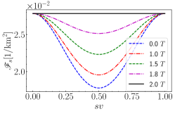
(a)

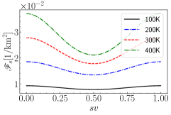
(b)

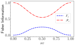
(c)

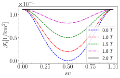
(d)

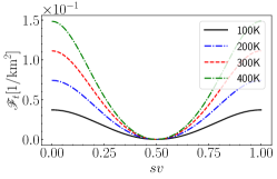
(e)

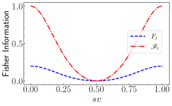
(f)

Figure 4: a) The QFI $\mathscr{F}_{s}$ with respect to $sv$ for various temperature difference $\Delta T$ for $T=300$ [K]. b) The QFI of estimating the separation of two-point sources as a function of $sv$ for different average temperatures. c) The QFI $\mathscr{F}_{s}$ (red dot-dashed) and CFI for heterodyne detection (Blue dashed) for estimating the separation of two-point sources as a function of $sv$. Both the QFI and the CFI scaled by $4\pi^{2}v^{2}\eta\kappa T$. d) The QFI $\mathscr{F}_{t}$ respect to $sv$ for various temperature difference $\Delta T$ for $T=300$ [K]. e) The QFI $\mathscr{F}_{t}$ respect to $sv$ for different average temperature $T$. For (a), (b), (d), and (e), the separation $\Delta r$ of the two receivers is fixed by 4 [m] and $\eta\sim 10^{-4}$. f) The QFI $\mathscr{F}_{t}$ (red dot-dashed) and CFI for heterodyne detection ${F}_{t}$ (Blue dashed) for estimating the separation of two-point source as a function of $sv$. Both the QFI and the CFI scaled by $32\pi^{2}v^{2}\eta\kappa T$.

In the limit $\Delta r\rightarrow 0$, the QFI for estimating $T$ becomes

$$\begin{split}\mathscr{F}_{T}\rightarrow\frac{2\pi a^{2}\kappa}{T\left(2\pi a^{2}\kappa T+R^{2}\right)}.\end{split}$$ (63)

Since we assume we are in a microwave regime $k_{B}T\gg\hbar\omega_{0}$, we can not take the limit $T\rightarrow 0$. Instead, we can verify that the QFI for estimating the temperature depends on the source size for a finite temperature. Now, for $T=$300 [K], and $30$ [km] source size we have the QFI around $2\times 10^{-5}$ [$1/\mathrm{K}^{2}$] which gives a very high standard deviation around 221 [K]. We show in the next section that the QFI also increases if we increase the number of spatial modes. For instance, for 20 receivers, we have QFI around $1.5\times 10^{-4}$ [$1/\mathrm{K}^{2}$], and the standard deviation is 79 [K] for a single measurement.

In the limit $\Delta r\rightarrow 0$, the CFI from heterodyne detection becomes

$$\begin{split}F_{T}\rightarrow\frac{4\pi^{2}a^{4}\kappa^{2}\left(\pi a^{2}\kappa T+R^{2}\right)\left(3\pi a^{2}\kappa T+R^{2}\right)}{\left(2\pi a^{2}\kappa T+R^{2}\right)^{4}}.\end{split}$$ (64)

To compare with the QFI we assume the brightness temperature $T=$ 300 [K], and source size $a=$ 30 [km]. This gives a CFI around $8\times 10^{-6}$ [$1/\mathrm{K}^{2}$] which give us a standard deviation around 350 [K]. Compared to the QFI information, the CFI is around 2.5 times smaller. Therefore, combining the spatial modes (receivers) and measuring photon number in the Fock basis of $\hat{d}_{1},\hat{d}_{2}$, as expected, is more advantageous even for estimating the temperature.

So far, we only gave the diagonal elements of the QFI matrix, relevant for estimating each parameter individually, assuming all other parameters are known. The single independent off-diagonal element of the QFI matrix regarding $a$ and $T$ is given in Eq. (90). In the limit $\Delta r\rightarrow 0$ it simplifies to

$$\mathscr{F}_{aT}=\frac{4\pi a\kappa}{2\pi a^{2}\kappa T+R^{2}}.$$ (65)

Then one can construct the QFI matrix to find the quantum Cramér-Rao bound for multiparameter estimation. Further, we can estimate the source location considering the two parameters $x_{0},y_{0}$. The QFI matrix elements for estimating the source locations can be written as

$$\begin{split}\mathscr{F}_{i_{0}j_{0}}=\frac{8\pi^{2}\Delta r^{2}\kappa TJ_{1}{}^{2}v_{i}v_{j}}{\pi{\Delta r}^{2}\left(\pi a^{2}\kappa T+R^{2}\right)-\kappa\lambda^{2}R^{2}TJ_{1}{}^{2}},\end{split}$$ (66)

where $i,j\in\{x,y\}$. The QFI for estimating the source location depends on source size and source temperature. Since the elements $\mathscr{F}_{i_{0}a}$ and $\mathscr{F}_{i_{0}T}$ of the QFI matrix are zero, source size and location can be estimated simultaneously. And the necessary phase delay for POVM can be found as $\delta_{i_{0}}=\delta+\pi/2$ from Eq. (96).

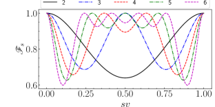
(a)

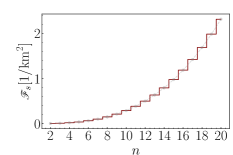
(b)

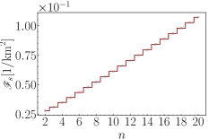
(c)

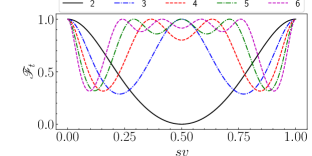
(d)

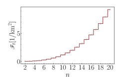
(e)

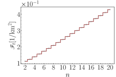
(f)

Figure 5: a) The QFI $\mathscr{F}_{s}$ as a function of $sv$ for $(2,3,4,5,6)$ mode interferometers and each curve is scaled by its maximum value which are $(\sim 1.7\times 10^{-3},\sim 6.9\times 10^{-3},\sim 17.3\times 10^{-3},\sim 34.7\times 10^{-3},\sim 60.8\times 10^{-3})[1/\mathrm{km}^{2}]$, respectively. b) The QFI $\mathscr{F}_{s}$ with respect to a number of interferometer modes $n$. d) The QFI $\mathscr{F}_{t}$ as a function of $sv$ for $(2,3,4,5,6)$ mode interferometers. Each curve is scaled by its maximum value which are $(\sim 0.67\times 10^{-2},\sim 2.78\times 10^{-2},\sim 6.96\times 10^{-2},\sim 13.9\times 10^{-2},\sim 24.3\times 10^{-2})[1/\mathrm{km}^{2}]$, respectively. e) The QFI $\mathscr{F}_{t}$ with respect to a number of interferometer modes $n$. (For all, the separation of two nearest receiver $\Delta r$ is 1m, and $\eta\sim 10^{-4}$. The maximum baseline is $\Delta r_{\mathrm{max}}=(n-1)\Delta r$.) c) The QFI $\mathscr{F}_{s}$ with respect to a number of interferometer modes $n$. f) The QFI $\mathscr{F}_{t}$ with respect to a number of interferometer modes $n$. For both (c) and (f), the maximum baseline is fixed by $\Delta r_{\mathrm{max}}=4$ [m], in this case, separation of two nearest receiver is $\Delta r=\Delta r_{\mathrm{max}}/(n-1)$, and $\eta\sim 10^{-4}$.

Spatial Resolution of Two Point Sources: Recently, the spatial resolution of two equally bright strong point sources was studied in [35] by considering the sources aligned parallel to the two-mode interferometer.

In this section, we consider a similar model with two circular disc sources on the surface of the source plane at locations ($\mathbf{r}_{1}=(x_{1},y_{1},R)$ and $\mathbf{r_{2}}=(x_{2},y_{2},R)$) but with different effective temperatures $T_{1}$ and $T_{2}$, and same sizes $a$. We assume that in the far field $\{x_{i},y_{i}\}\ll R$ and $a\ll R$. We analyze two cases; when the sources are aligned or not aligned with the two receivers. For two circular sources with equal size, the temperature distribution over the surface can be written as

$$T_{\mathrm{eff}}(x,y)=\sum_{i=\{1,2\}}T_{i}\mathrm{circ}({x-x_{i},y-y_{i}}).$$ (67)

Then we can define the four parameters that we want to estimate as: source separation ($s_{x}=x_{1}-x_{2}$), ($s_{y}=y_{1}-y_{2}$) and centroid of the two sources ($t_{x}=(x_{1}+x_{2})/2$), ($t_{y}=(y_{1}+y_{2})/2$). In Appendix E, we express the QFI matrix elements for all four parameters. Since these equations are quite complicated, we check the important limits. Since we want to resolve the two-point sources even for very small separation, we check the limit, $s_{x},s_{y}\rightarrow 0$. Then we have QFI matrix elements for estimating the source separation as $\mathscr{F}_{s_{i}}\rightarrow{4\pi^{2}v_{i}^{2}\eta\kappa T}$ and $\mathscr{F}_{s_{x}s_{y}}\rightarrow{4\pi^{2}v_{x}v_{y}\eta\kappa T}$, if $T_{1}=T_{2}=T$.

If we assume two sources aligned parallel to the two-mode interferometer ($y_{1}=0,y_{2}=0$ and $\varphi=0\rightarrow v=v_{x}=\Delta r/(R\lambda)$ and $s_{x}\rightarrow s,\quad t_{x}\rightarrow t$) we can simplify our problem to a single dimension. We show the dependence of the QFI matrix elements on average temperature ($T=(T_{1}+T_{2})/2$) and temperature difference $\Delta T=T_{1}-T_{2}$ assuming $T_{1}\geq T_{2}$. In Fig. (4b), we plot $\mathscr{F}_{s}$ with respect to $sv$ for different average temperatures. As expected, when the temperature increases, the QFI for estimating the separation also increases. For $T=300$ [K] and $\Delta r=4$ [m], we have a QFI around $0.027\;[1/\mathrm{km}^{2}]$ which corresponds to a standard deviation of 6 [km] for only two receivers for the separation estimation. In Fig. (4a), we see that, as we increase the temperature difference between the two-point sources, the QFI becomes less oscillatory and at $\Delta T\rightarrow 2T$, the oscillatory behavior disappears. In the limit $\Delta T\rightarrow 2T$, or $s\rightarrow 0$ the QFI for estimating $s$ becomes

$$\begin{split}\mathscr{F}_{s}\rightarrow{4\pi^{2}v^{2}\eta\kappa T}\,,\end{split}$$ (68)

which is the limit given by the solid black line in Fig. (4a). We calculated the CFI from heterodyne detection to estimate the source separation in Eq. (114). If the size of the sources is very small and in the limit $\eta\kappa T\ll 1$ the CFI for estimating the source separation simplifies to

$$\begin{split}F_{s_{i}}\xrightarrow{\eta\kappa T\ll 1}8\pi^{2}\eta^{2}\kappa^{2}T^{2}v_{i}^{2}\sin^{2}(\pi(s_{x}v_{x}+s_{y}v_{y})).\end{split}$$ (69)

When the source separation goes to zero ($s_{x},s_{y}\rightarrow 0$), $F_{s_{i}}$ tends to zero. We compare the QFI with CFI in Eq. (114) from heterodyne detection in Fig. (4c). As we can see, the CFI goes to zero for small source separation. Therefore, we can conclude that Rayleigh’s curse limits heterodyne detection. The POVM from the SLD eliminates that limitation. We give the elements of the matrix $\mathbf{M}_{s}$, $g^{1}_{s}$ and $g^{2}_{s}$ in Appendix E. The phase difference for combining two spatial modes of the interferometer can be found as $\delta_{s}=2\pi(t_{x}v_{x}+t_{y}v_{y})-\pi$. Assuming the alignment of the spatial mode separation parallel to source separation, it becomes $\delta_{s}=2\pi tv-\pi$.

The QFI matrix elements for estimating the centroid is given in Eq. (106). We assume that the two sources aligned again parallel to two spatial modes of the interferometer ($y_{1}=0,y_{2}=0$ and $\varphi=0\rightarrow v=v_{x}=\Delta r/(R\lambda)$ and $s_{x}\rightarrow s,\quad t_{x}\rightarrow t$) and $\mathscr{F}_{t_{x},t_{x}}\rightarrow\mathscr{F}_{t}$. In Fig. (4e), we see that the $\mathscr{F}_{t}$ increases when we increase the temperature. For $T=300$ [K] and $\Delta r=4$ [m], we have a QFI $\mathscr{F}_{t}\sim 0.11\;[1/\mathrm{km}^{2}]$ which corresponds to a standard deviation of 3 [km] for estimating the centroid. When $sv\sim 0.5$, $\mathscr{F}_{t}$ goes to zero for equally bright sources. In Fig. (4d) we see that it is not zero for $sv\sim 0.5$, if $\Delta T\neq 0$, and the oscillation of $\mathscr{F}_{t}$ decreases when we increase the temperature difference. In the limit $s\rightarrow 0$, $\mathscr{F}_{t}$ simplifies to

$$\begin{split}\mathscr{F}_{t}\rightarrow{32\pi^{2}v^{2}\eta\kappa T}\end{split}$$ (70)

for $\Delta T=0$. The CFI for heterodyne detection is given in Eq. (113). For small sources we consider again the limit $\eta\kappa T\ll 1$, and we ignore the higher order terms of $\eta\kappa T$. Then we have

$$\begin{split}F_{t_{i}}\xrightarrow{\eta\kappa T\ll 1}32\pi^{2}\eta^{2}\kappa^{2}T^{2}{v_{i}}^{2}\cos^{2}(\pi({s_{x}}{v_{x}}+{s_{x}}{v_{y}})).\end{split}$$ (71)

If the source separation goes to zero ($s_{x},s_{y}\rightarrow 0$), we still have a finite $F_{t_{i}}$, unlike the CFI for source separation. In Fig. (4f), we compare $\mathscr{F}_{t}$ with $F_{t_{i}}$. When the source separation goes to zero, both Fisher information goes to a constant, and both go to zero at $sv\rightarrow 0.5$. However, the QFI is five times larger than the CFI from heterodyne detection. Again the phase difference for the POVM from the SLD can be found as $\delta_{t}=2\pi tv+\pi/2$.

III.3 1D $n$-mode interferometer arrays

The previous section considered a two-mode interferometer for analytical calculations and compared the QFI with its POVM and CFI for heterodyne detection. To compare our results with SMOS, we extend the two-mode interferometer to a 1D array of $n$ single-mode receivers. We investigate numerically how the QFI changes when increasing the number $n$ of interferometer modes. We assume the receiver array aligned with the $x$ axis on the detection plane and denote the maximum baseline separation of the two most distant receivers by $\Delta r_{\mathrm{max}}$.

Resolution of Two Point Sources for n mode interferometer array: We assume that both sources have the same sizes and temperatures ($\Delta T=0$ and $T_{1}=T_{2}=T$) and that they are parallel to the receiver array. In Fig. (5a), we see that when we increase the number of receivers, the behavior of $\mathcal{F}_{s}$ changes. It is still oscillatory as a function of $sv$ with a period of $2\pi$. However, for each oscillation, we have $n-2$ additional maxima. Moreover, in Fig. (5b), we see that $\mathcal{F}_{s}$ increases gradually when we increase the number of receivers and the maximum baseline increases as $\Delta r_{\mathrm{max}}=(n-1)\Delta r$. For $\Delta r=1$ [m] and $T=300$ [K], the standard deviation for estimating the source separation is $\sim 23$ [km] for the two-mode interferometer. For the 20 mode interferometer, we find a standard deviation of around $0.65$ [km]. Further, if we keep the baseline fixed as $4$ [m], the QFI increases linearly with the number of receivers, as we can see in Fig. (5c). In this case, for a two-mode interferometer, we have a standard deviation of around $6$ [km], and for a 20-mode interferometer, we have $3$ [km].

We also checked the centroid estimation for the $n$ mode interferometer. It leads to similar results as for source separation. From Fig. (5d) we see that for $sv=0.5$ the centroid uncertainty for the two-mode receiver diverges ($\mathscr{F}_{t}\sim 0$ at $sv\sim 0.5$). This is no longer the case for the array of $n$ receivers. In Fig. (5e), we see that $\mathscr{F}_{t}$ also increases with the number of modes. For the two modes, the standard deviation for estimating the centroid was $\sim 12$ [km]. For the 20 modes, we have a standard deviation of around 0.32 [km] considering $\Delta r=1$ [m], and $\Delta r_{\mathrm{max}}=(n-1)\Delta r$ for average temperature $T=300$ [K]. If we keep the baseline fixed, as we can see from the Fig. (5f), $\mathscr{F}_{t}$ increases linearly by $n$. By fixing the $\Delta r_{\mathrm{max}}=4$ [m], we have a standard deviation of $\sim 3$ [km] for the two mode interferometer; for 20 modes we have a standard deviation of $\sim 1.5$ [km]. Thus, instead of sampling the state in time, we can increase the number of receivers to increase the QFI, and both methods can be combined as well.

Spatial Resolution of Single Circular Source for n mode interferometer array: To analyze the effect of $n$ for source size estimation, we consider a single circular source as given in Eq. (46). In Fig. (6), we show how the QFI for estimating $a$ changes with $n$. For $a\rightarrow 0$, $\mathscr{F}_{a}$ increases linearly with $n$.

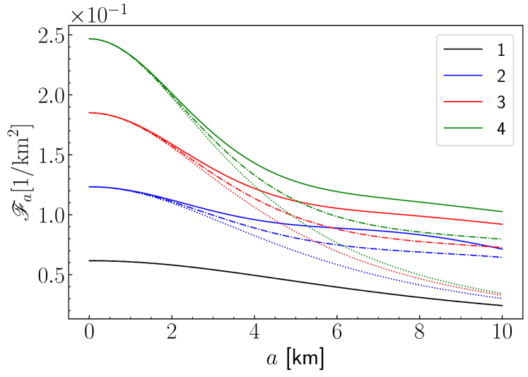
Figure 6: a) The QFI $\mathscr{F}_{a}$ as a function of $a$ for $(1,2,3,4)$ mode interferometers, which are given by black, blue, red, and yellow lines, respectively. The maximum baseline difference is given by; $\Delta r_{\mathrm{max}}\rightarrow 0$ for dotted lines, $\Delta r_{\mathrm{max}}=4$ [m] for dashed lines, and $\Delta r_{\mathrm{max}}=6$ [m] for solid lines. The black solid line corresponds to single receiver. $T=300$ [K].

We have $\mathscr{F}_{a}\sim 6.16\times 10^{-2}\;\mathrm{[1/km^{2}]}$ for single receiver which corresponds to a standard deviation of 4 [km] and for higher $n$, we have approximately $\mathscr{F}_{a}\propto n$ for small values of $a$. If we have an array of 20 receivers, $\mathscr{F}_{a}\sim 1.23\;\mathrm{[1/km^{2}]}$ which gives a standard deviation of 0.9 [km] for estimating $a$. When we increase the source size $a$, we see that there is extra information coming from the phase differences as given by the solid lines for $\Delta r_{\mathrm{max}}=6$ [m] and dashed lines for $\Delta r_{\mathrm{max}}=4$ [m]. One can also see that as expected the dotted lines, corresponding to the limit $\Delta r_{\mathrm{max}}\rightarrow 0$, get close to the solid black line, which corresponds to a single receiver, for large values of $a$.

To linearly combine these modes, one can calculate the elements of the matrix $\mathbf{M}_{i}$ numerically. Each normalized eigenvector of $\mathbf{M}_{i}$ maps to a set of operators $\bar{\mathbf{d}}$ by linear combination of the operators in $\bar{\mathbf{b}}$ with corresponding weights and phases. One can design a setup using these weights and phases in the eigenvectors to achieve the resolutions for a chosen parameter given in this section.

IV Conclusion

In summary, we studied possible quantum advantages in passive microwave remote sensing. Starting from a microscopic current density distribution in the source plane corresponding to a position-dependent brightness temperature $T_{\mathrm{eff}}(x,y)$, we derived the general partially coherent state received by an array of receivers. From the dependence of that partially coherent states on parameters that characterize the sources, such as the radius $a$ and brightness temperature $T$ of a uniform circular source, we obtained the quantum Fisher information and hence the quantum Cramér-Rao bound for the smallest possible uncertainty with which these parameters can be estimated based on measurements of the multi-mode state of the receivers. We showed how the optimal measurements allowing one to estimate a single parameter can be obtained for a general antenna array with receivers placed at arbitrary positions. In general, the optimal measurements correspond to photon-detection in certain detector modes that can be obtained from the original receiver modes by mode mixing via beam-splitters and phase shifters. For single-mode and two-mode interferometers, we gave explicit analytical results for the best possible resolution of one or two uniform circular sources, both in $a$ and $T$ and demonstrated a clear quantum advantage over the classical strategy corresponding to direct heterodyne measurements of the receiver modes. In the limit of small source sizes, we recover known results for the measurement of the centroid and separation of two-point sources. We benchmarked our results with the performance of the SMOS mission, which achieves about 35 km resolution with 69 antennas deployed on three four-meter long arms arranged in a Y-shape, operating at 21 cm the wavelength, and flying at a height of 758 km above Earth. As an example, we showed that by using the optimal measurements, a single arm of length 4 m with 20 antennas and a single measurement would allow a spatial resolution of about 1.5  km. I.e. with a smaller satellite, a more than 20-fold increase of resolution compared to SMOS could be achieved. By increasing the size of the array to 19 m, the 20 antennas should give rise to a spatial resolution down to 300 m. Substantially better resolutions can be achieved if we allow more measurements. If we assume that the number of samples is given by the time the satellite flies over the object whose size one wants to estimate divided by the inverse bandwidth, even with a single receiver a spatial resolution down to a few meters and a radiometric resolution of a fraction of a Kelvin become possible in principle.
Our results generalize previous approaches to quantum-enhanced imaging based typically on weak sources (photon numbers on average smaller than 1 per mode) or point sources, and pave the way to quantum metrological sensitivity enhancements in real-world scenarios in passive microwave remote sensing. Several challenges remain. Experimentally, single-photon detection in the microwave regime is still difficult but starts to become available [72]. It requires very low temperatures for operating superconducting qubits that would have to be maintained on a long time scale on the satellite. From the theoretical side, an extension to a many-parameter regime requiring adaption of the optimal measurements will be crucial for true imaging. Post-measurement beam synthesis that is common in interferometric astronomy does not work here, as already the detection modes depend on the pixel in the image that one wants to focus on. Nevertheless, the substantial quantum advantages demonstrated here theoretically in a relatively simple but real-world scenario give hope that quantum metrology can help to significantly improve the resolution of passive Earth observation schemes, with corresponding positive impact on the data available for feeding climate models, weather forecasts, and forecasts of floodings.

Appendix A Brightness Temperature and Current Density Fluctuations

The number of photons that pass through a certain receiver area $A_{D}$ in a certain time $t_{D}$ can be found from $\bar{n}=A_{D}t_{D}\Phi$, where $\Phi$ is the photon flux. For a given intensity $I$, the photon flux for frequency $\omega_{0}$ can be found by $\Phi={I}/({\hbar\omega_{0}})$. If the total energy density on the receiver is $U_{D}$, then the intensity can be written as $I=U_{D}c$. Then $\bar{n}$ becomes $\bar{n}={A_{D}t_{D}U_{D}c}/({\hbar\omega_{0}})$. In the microwave regime $\hbar\omega\ll k_{B}T$, the energy density (energy per unit volume per frequency) from black body radiation at frequency $\omega$ with a temperature distribution $T(x,y)$ on the surface of radiation at the $i$-th receiver position is given by [43]

$$u_{D}(\omega)=\frac{k_{B}}{2\pi^{3}c^{3}}\int dxdy\omega^{2}\frac{T_{B}(x,y)\cos\tilde{\theta}(x,y)}{|\mathbf{r}-\mathbf{r}_{i}|^{2}},$$ (72)

where the brightness temperature is defined as $T_{B}(x,y)\equiv T(x,y)B(x,y;\omega,\tilde{\theta},\tilde{\varphi})$, Earth is rather a grey than a black body, therefore the emissivity $B(x,y;\omega,\tilde{\theta},\tilde{\varphi})$ of the patch in the direction of the satellite given by polar and azimuthal angles is introduced. One can take the integral over $\omega$ using the filter function in Eq. (21) to find the total energy density (energy per volume) and it becomes

$$U_{D}=\frac{k_{B}\omega_{0}^{2}B}{2\pi^{3}c^{3}}\int dxdy\frac{T_{B}(x,y)\cos\tilde{\theta}(x,y)}{|\mathbf{r}-\mathbf{r}_{i}|^{2}}.$$ (73)

Then the photon number on the receiver becomes

$$\bar{n}=\frac{2k_{B}}{\pi\hbar\omega_{0}}\left(\frac{A_{D}}{\lambda^{2}}\right)(t_{D}B)\int dxdy\frac{T_{B}(x,y)\cos\tilde{\theta}(x,y)}{|\mathbf{r}-\mathbf{r}_{i}|^{2}}.$$ (74)

For simplicity of the receivers scattering function, we set $A_{D}\sim\lambda^{2}$ and $t_{D}\sim 1/B$. Comparing Eq. (74) with Eq. (29), we define $\braket{}{\tilde{{j}}_{t,i}\left(\mathbf{r},{\omega}\right)}{{}^{2}}\equiv K_{1}T_{\mathrm{B}}(x,y)\cos\tilde{\theta}(x,y)\delta(z-R)$ with a constant $K_{1}=32\tau_{c}k_{B}/(3l_{c}^{3}\mu_{0}c)$ which agrees with the result in Ref. [43].

Appendix B The general QFI and the elements of the matrix M for a two-mode interferometer

In this section, we give the general results for the elements of the QFI and the matrix $\mathbf{M}_{i}$ for a two-mode interferometer, assuming that all the elements of the covariance matrix depend on the parameter $\mu_{i}$ that we want to estimate. Using the covariance matrix for a two-mode interferometer one finds the QFI matrix elements as

$$\begin{split}\mathscr{F}_{ij}=&\frac{8}{\mathscr{D}}\left[\partial_{i}\xi^{*}\partial_{j}\xi((1-4\chi^{2})^{2}-4(1+4\chi^{2})|\xi|^{2})\right.+\partial_{i}\xi\partial_{j}\xi^{*}((1-4\chi^{2})^{2}-4(1+4\chi^{2})|\xi|^{2})\\ +&4\xi\partial_{i}\xi^{*}(\xi\partial_{j}\xi^{*}(1+4\chi^{2}-4|\xi|^{2})+2\chi\partial_{j}\chi(1-4\chi^{2}+4|\xi|^{2}))+4\xi^{*}\partial_{i}\xi(\xi\partial_{j}\xi^{*}(1+4\chi^{2}-4|\xi|^{2})\\ +&2\chi\partial_{j}\chi(1-4\chi^{2}+4|\xi|^{2}))+2\partial_{i}\chi(-1+4\chi^{2}-4|\xi|^{2})(-4\chi(\xi\partial_{j}\xi^{*}+\xi^{*}\partial_{j}\xi)+\left.\partial_{j}\chi(-1+4\chi^{2}+4|\xi|^{2}))\right],\end{split}$$ (75)

where the denominator is given by

$$\begin{split}\mathscr{D}=(-1+4\chi^{2}-4|\xi|^{2})(16\chi^{4}+(1-4|\xi|^{2})^{2}-8\chi^{2}(1+|\xi|^{2})).\end{split}$$ (76)

Using the SLD given in Eq. (38) we find the diagonal elements of the matrix $\mathbf{M}_{i}$ as

$$\begin{split}g^{1}_{i}=\frac{2\left(4{\partial_{i}\chi}|\xi|^{2}+4{\partial_{i}\chi}\chi^{2}-4{\partial_{i}\xi}\xi^{*}\chi-4{\partial_{i}\xi^{*}}\xi\chi-{\partial_{i}\chi}\right)}{16\chi^{4}-8\chi^{2}(4|\xi|^{2}+1)+(1-4|\xi|^{2})^{2}},\end{split}$$ (77)

where the two diagonal elements are the same due to the symmetry with respect to the center of the two receivers, and

$$\begin{split}g^{2}_{i}&=\frac{2}{\mathscr{D}}\left[-{\partial_{i}\xi}\left(16|\xi|^{2}\chi^{2}+4|\xi|^{2}-16\chi^{4}+8\chi^{2}-1\right)\right.-{\partial_{i}\xi^{*}}\left(4\xi^{2}(4|\xi|^{2}-1)-16\xi^{2}\chi^{2}\right)\left.-{\partial_{i}\chi}\left(32\xi\chi^{3}-8\xi\chi(4|\xi|^{2}+1)\right)\right],\end{split}$$ (78)

where $\mathscr{D}$ is given in Eq. (76)

Appendix C The POVM for heterodyne detection

The POVM for heterodyne detection is given in Ref. [34], and the CFI analyzed for the weak thermal sources. Here we briefly introduce the POVM for heterodyne detection. Then, we compare our results for the QFI with the CFI for heterodyne detection. The POVM is given as

$$\begin{split}E(\nu_{1},\nu_{2})=\frac{1}{\pi^{2}}|\nu_{1},\nu_{2}\rangle\langle\nu_{1},\nu_{2}|,\end{split}$$ (79)

where $|\nu_{1},\nu_{2}\rangle$ is a coherent state with normalization given by $\int d^{2}\nu_{1}d^{2}\nu_{2}E(\nu_{1},\nu_{2})=\mathds{1}$. The covariance matrix for a two-mode interferometer is given in Eq. (56). Using the corresponding state for the two-mode interferometer we can find the observation probability for any parameter $\mu_{i}$, in terms of the elements of the covariance matrix as

$$\begin{split}&P(\nu_{1},\nu_{2}|\mu_{i})=\frac{1}{\pi^{2}((1+\bar{n})^{2}-|\xi|^{2})}\exp\left[{\frac{(-|\nu_{1}|^{2}-|\nu_{1}|^{2})(1+\bar{n})+\xi\nu_{1}^{*}\nu_{2}+\xi^{*}\nu_{2}^{*}\nu_{1}}{(1+\bar{n})^{2}-|\xi|^{2}}}\right].\end{split}$$ (80)

The Fisher information for the parameter $\mu_{i}$ can be found as

$$\begin{split}F_{i}&=\int d^{2}\nu_{1}d^{2}\nu_{2}\frac{1}{P(\nu_{1},\nu_{2}|\mu_{i})}\left(\frac{\partial P(\nu_{1},\nu_{2}|\mu_{i})}{\partial\mu_{i}}\right)^{2}\\ &=\int d^{2}\nu_{1}d^{2}\nu_{2}{P(\nu_{1},\nu_{2}|\mu_{i})}f(\nu_{1},\nu_{2})\\ &=\braket{f(\nu_{1},\nu_{2})},\end{split}$$ (81)

where $f(\nu_{1},\nu_{2})$ is a polynomial function of second and fourth order correlations of $\nu_{1}$ and $\nu_{2}$, defined as

$$\begin{split}f(\nu_{1},\nu_{2})\equiv\left(\partial_{\mu_{i}}\log\left(P(\nu_{1},\nu_{2}|\mu_{i})\right)\right)^{2}=\frac{1}{(P(\nu_{1},\nu_{2}|\mu_{i}))^{2}}\left(\frac{\partial P(\nu_{1},\nu_{2}|\mu_{i})}{\partial\mu_{i}}\right)^{2}.\end{split}$$ (82)

With Wick’s theorem for Gaussian states, the fourth order statistic can be written as

$$\begin{split}\braket{x_{1}x_{2}x_{3}x_{4}}=\braket{x_{1}x_{2}}\braket{x_{3}x_{4}}+\braket{x_{1}x_{3}}\braket{x_{2}x_{4}}+\braket{x_{1}x_{4}}\braket{x_{2}x_{3}},\end{split}$$ (83)

where $x_{i}\in\{\nu_{1},\nu_{1}^{*},\nu_{2},\nu_{2}^{*}\}$. We can also write $\braket{}{{\nu_{1}}}{{}^{2}}=\braket{}{{\nu_{2}}}{{}^{2}}=1+\bar{n}$ and $\braket{\nu_{1}^{*}\nu_{2}}=\xi$, $\braket{\nu_{2}^{*}\nu_{1}}=\xi^{*}$.

Appendix D The uniform circular source for a two-mode interferometer

We find the elements of the covariance matrix describing the state of two-mode interferometers in Eq. (56). Then for a circular source with size $a$ located at position $(x_{0},y_{0},R)$ with the assumption $x_{0},y_{0}\ll R$ in the source plane we have

$$\begin{split}\bar{n}&=\frac{\kappa T}{R^{2}}\int dxdy\mathrm{circ}({x-x_{0},y-y_{0}}),\\ &=\frac{\pi a^{2}\kappa T}{R^{2}},\end{split}$$ (84)

and $\chi$ and $\xi$ become

$$\begin{split}\chi=\frac{1}{2}+\frac{\pi a^{2}\kappa T}{R^{2}},\end{split}$$ (85)

$$\begin{split}\xi=\braket{b_{2}^{\dagger}b_{1}}&=\frac{\kappa T}{R^{2}}\int dxdy\mathrm{circ}({x-x_{0},y-y_{0}})\exp\left(2\pi i(xv_{x}+yv_{y})\right)\\ &=\frac{\kappa Ta^{2}}{R^{2}}\frac{J_{1}\left(2\pi a\sqrt{v_{x}^{2}+v_{y}^{2}}\right)}{a\sqrt{v_{x}^{2}+v_{y}^{2}}}\exp\left(2\pi i(x_{0}v_{x}+y_{0}v_{y})\right),\end{split}$$ (86)

where $v_{x}=\Delta r\cos\varphi/(\lambda R)$, $v_{y}=\Delta r\sin\varphi/(\lambda R)$, with $\mathbf{\Delta r}=\Delta r(\cos\varphi,\sin\varphi,0)$. Note that $\sqrt{v_{x}^{2}+v_{y}^{2}}=\Delta r/(\lambda R)$.

The Quantum Fisher Information: The uniform circular source

We found the QFI for estimating $a$ is as

$$\begin{split}\mathscr{F}_{a}=&\frac{8\pi^{2}a\Delta r^{2}\kappa T}{\mathscr{D}_{a}}\left[\pi a{\Delta r}^{2}(\pi a^{2}\kappa T+R^{2})(J_{0}^{2}+1)-2{\Delta r}\lambda R(2\pi a^{2}\kappa T+R^{2})J_{0}J_{1}+a\kappa\lambda^{2}R^{2}T(J_{0}^{2}+1)J_{1}^{2}\right],\end{split}$$ (87)

where

$$\begin{split}\mathscr{D}_{a}&=\left(\pi^{2}a^{2}\Delta r^{2}-\lambda^{2}R^{2}J_{1}^{2}\right)\left(\Delta r^{2}\left(\pi a^{2}\kappa T+R^{2}\right)^{2}-\kappa^{2}\lambda^{2}R^{2}T^{2}J_{1}^{2}\right),\end{split}$$ (88)

and $J_{i}\left(\frac{2a\Delta r\pi}{R\lambda}\right)$ are the Bessel functions of the first kind and $i$-th order. The QFI for estimating $T$ becomes

$$\begin{split}\mathscr{F}_{T}&=\frac{2\kappa a^{2}\left(\pi\Delta r^{2}\left(\pi a^{2}\kappa T+R^{2}\right)-\kappa\lambda^{2}R^{2}TJ_{1}^{2}\right)}{T\left(\Delta r^{2}\left(\pi a^{2}\kappa T+R^{2}\right)^{2}-a^{2}\kappa^{2}\lambda^{2}R^{2}T^{2}J_{1}{}^{2}\right)}\,.\end{split}$$ (89)

The other elements regarding the source size and the temperature of the circular source can be found as

$$\begin{split}\mathscr{F}_{aT}=\frac{4\pi a{\Delta r}\kappa\left({\Delta r}\left(\pi a^{2}\kappa T+R^{2}\right)-a\kappa\lambda RTJ_{0}J_{1}\right)}{{\Delta r}^{2}\left(\pi a^{2}\kappa T+R^{2}\right)^{2}-a^{2}\kappa^{2}\lambda^{2}R^{2}T^{2}J_{1}{}^{2}}.\end{split}$$ (90)

The QFI matrix elements for estimating the source locations can be written as

$$\begin{split}\mathscr{F}_{i_{0}j_{0}}=\frac{8\pi^{2}R^{2}\lambda^{2}\kappa TJ_{1}{}^{2}v_{i}v_{j}}{\pi{\Delta r}^{2}\left(\pi a^{2}\kappa T+R^{2}\right)-\kappa\lambda^{2}R^{2}TJ_{1}{}^{2}},\end{split}$$ (91)

where $i,j\in\{x,y\}$.

The elements of the matrix $\mathbf{M}_{i}$ for a two-mode interferometer: The uniform circular source

To combine two modes of the receivers for the optimum measurements, we calculate $\delta$ as given in Eq.(58). We find the matrix elements of $\mathbf{M}_{a}$ as

$$\begin{split}g^{1}_{a}&=\frac{2\pi{\Delta r}^{2}R^{2}}{\mathscr{D}_{a}}(\pi a{\Delta r}^{2}(\pi a^{2}\kappa T+R^{2})+\lambda RJ_{1}(a\kappa\lambda RTJ_{1}-{\Delta r}(2\pi a^{2}\kappa T+R^{2})J_{0})),\end{split}$$ (92)

$$\begin{split}g^{2}_{a}&=\frac{2\pi{\Delta r}^{2}R^{2}}{\mathscr{D}_{a}}(aJ_{0}(\pi{\Delta r}^{2}(\pi a^{2}\kappa T+R^{2})+\kappa\lambda^{2}R^{2}TJ_{1}{}^{2})-{\Delta r}\lambda R(2\pi a^{2}\kappa T+R^{2})J_{1})e^{-i\delta},\end{split}$$ (93)

where $\delta=v_{x}x_{0}+v_{y}y_{0}$. For the temperature estimation we get the elements of $\mathbf{M}_{T}$ as

$$\begin{split}g^{1}_{T}&=\frac{{\Delta r}^{2}R^{2}\left(\pi a^{2}\kappa T+R^{2}\right)}{{\Delta r}^{2}T\left(\pi a^{2}\kappa T+R^{2}\right)^{2}-a^{2}\kappa^{2}\lambda^{2}R^{2}T^{3}J_{1}^{2}},\end{split}$$ (94)

$$\begin{split}g^{2}_{T}&=-\frac{a{\Delta r}\kappa\lambda R^{3}J_{1}e^{-i\delta}}{a^{2}\kappa^{2}\lambda^{2}R^{2}T^{2}J_{1}^{2}-{\Delta r}^{2}\left(\pi a^{2}\kappa T+R^{2}\right)^{2}}.\end{split}$$ (95)

Finally, for the source location we found

$$\begin{pmatrix}g^{2}_{x_{0}}\\ g^{2}_{y_{0}}\end{pmatrix}=-\frac{2\pi{\Delta r}^{2}R^{2}J_{1}e^{i(-\delta+\pi/2)}}{a\left(\pi{\Delta r}^{2}\left(\pi a^{2}\kappa T+R^{2}\right)-\kappa\lambda^{2}R^{2}TJ_{1}^{2}\right)}\begin{pmatrix}\cos(\varphi)\\ \sin(\varphi)\end{pmatrix},$$ (96)

and $g^{1}_{x_{0}}=g^{1}_{y_{0}}=0$.

The classical Fisher information for heterodyne detection: The Uniform Circular Source

Since we calculated the elements of the covariance matrix in Eq. (84) and Eq. (85) we can calculate Eq. (80) and Eq. (82). Using the CFI for the heterodyne detection in Eq. (81), we can write the result for estimating the source size as

$$\begin{split}F_{a}=&\frac{8\pi^{2}a^{2}\kappa^{2}T^{2}\Delta r^{3}(\pi a^{2}\kappa T+R^{2})}{D_{a}}[4a^{5}\kappa^{5}\lambda^{5}R^{5}T^{5}J_{0}J_{1}{}^{5}-2a^{2}{\Delta r}^{3}\kappa^{2}\lambda^{2}R^{2}T^{2}(\pi a^{2}\kappa T+R^{2})^{3}(J_{0}{}^{2}+1)J_{1}{}^{2}\\ &+{\Delta r}^{5}(\pi a^{2}\kappa T+R^{2})^{5}(J_{0}{}^{2}+1)-4a{\Delta r}^{4}\kappa\lambda RT(\pi a^{2}\kappa T+R^{2})^{4}J_{0}J_{1}\\ &-7a^{4}{\Delta r}\kappa^{4}\lambda^{4}R^{4}T^{4}(\pi a^{2}\kappa T+R^{2})(J_{0}{}^{2}+1)J_{1}{}^{4}+16a^{3}{\Delta r}^{2}\kappa^{3}\lambda^{3}R^{3}T^{3}(\pi a^{2}\kappa T+R^{2})^{2}J_{0}J_{1}{}^{3}],\end{split}$$ (97)

with

$$\begin{split}D_{a}={(\Delta r^{2}(\pi a^{2}\kappa T+R^{2})^{2}-{a^{2}\kappa^{2}\lambda^{2}R^{2}T^{2}J_{1}{}^{2}}){}^{4}}.\end{split}$$ (98)

The estimation of the temperature becomes

$$\begin{split}F_{T}&=\frac{2a^{2}{\Delta r}^{2}\kappa^{2}(\pi a^{2}\kappa T+R^{2})}{D_{T}}(\pi^{2}a^{2}{\Delta r}^{6}(\pi a^{2}\kappa T+R^{2})^{5}-a^{4}\kappa^{4}\lambda^{6}R^{6}T^{4}(3\pi a^{2}\kappa T+7R^{2})J_{1}{}^{6}\\ &+{\Delta r}^{4}\lambda^{2}R^{2}(\pi a^{2}\kappa T+R^{2})^{3}(-5\pi^{2}a^{4}\kappa^{2}T^{2}-2\pi a^{2}\kappa R^{2}T+R^{4})J_{1}{}^{2}+a^{2}{\Delta r}^{2}\kappa^{2}\lambda^{4}R^{4}T^{2}(7\pi^{3}a^{6}\kappa^{3}T^{3}\\ &+19\pi^{2}a^{4}\kappa^{2}R^{2}T^{2}+10\pi a^{2}\kappa R^{4}T-2R^{6})J_{1}{}^{4}),\end{split}$$ (99)

where

$$\begin{split}D_{T}={\left({\Delta r}^{2}\left(\pi a^{2}\kappa T+R^{2}\right)^{2}-a^{2}\kappa^{2}\lambda^{2}R^{2}T^{2}J_{1}{}^{2}\right){}^{4}}.\end{split}$$ (100)

Appendix E Two point sources for a two-mode interferometer

The temperature distribution of two circular sources with equal size $a$ at locations $(x_{1},y_{1},R)$ and $(x_{2},y_{2},R)$ is given in Eq. (67). We assume that $\{|x_{i}|,|y_{i}|,a\}\ll R$. The elements of the covariance matrix in Eq. (56) for two point sources with different temperature can be found using Eq. (31), Eq. (32) and Eq. (67) as

$$\begin{split}\chi&=\frac{1}{2}+\sum_{i}\frac{\pi a^{2}\kappa T_{i}}{R^{2}}=\frac{1}{2}+\frac{2\pi a^{2}\kappa T}{R^{2}}\\ &=\frac{1}{2}+2\eta\kappa T,\end{split}$$ (101)

where $\eta=\pi a^{2}/R^{2}$, and

$$\begin{split}\xi=\braket{b^{\dagger}_{1}b_{2}}&=\frac{\kappa\pi a^{2}}{R^{2}}\frac{2{J_{1}\left(\frac{2\pi a\Delta r}{R\lambda}\right)}}{\frac{2\pi a\Delta r}{R\lambda}}(T_{1}e^{2\pi i(v_{x}x_{1}+v_{y}y_{1})}+T_{2}e^{2\pi i(v_{x}x_{2}+v_{y}y_{2})})\\ &=\frac{\kappa\eta\eta_{2}}{2}((2T-\Delta T)e^{2\pi i(v_{x}x_{1}+v_{y}y_{1})}+(2T+\Delta T)e^{2\pi i(v_{x}x_{2}+v_{y}y_{2})}),\end{split}$$ (102)

where the average temperature is defined as $T\equiv(T_{1}+T_{2})/2$, and the temperature difference of the sources as $\Delta T\equiv T_{2}-T_{1}$ with $T_{2}\geqslant T_{1}$ assumed, while the parameter $\eta_{2}$ is given by

$$\eta_{2}=\frac{2{J_{1}\left(\frac{2\pi a\Delta r}{R\lambda}\right)}}{\frac{2\pi a\Delta r}{R\lambda}},$$ (103)

which is related to the source size. In Fig. (7), we can see the behavior of $\eta_{2}$ with respect to the source size. For point sources one can approximate $\eta_{2}\approx 1$.

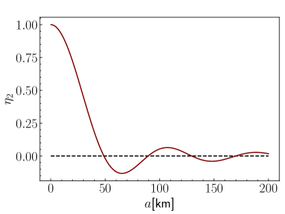
Figure 7: Plot showing the behavior of $\eta_{2}$ with respect to the radius of the circular disc source.

The Quantum Fisher Information: Two Point Sources

We found the elements of the QFI matrix for estimating the source separation as

$$\begin{split}\mathscr{F}_{s_{i}s_{j}}&=\frac{2\pi^{2}\eta\kappa{v_{i}}{v_{j}}}{\mathscr{D}_{s_{x}s_{y}}}(\eta^{2}\kappa^{2}(4T^{2}-{\Delta T}^{2})((4T^{2}-{\Delta T}^{2})\cos(4\pi({s_{x}}{v_{x}}+{s_{y}}{v_{y}}))+16T^{2}\cos(2\pi({s_{x}}{v_{x}}+{s_{y}}{v_{y}})))\\ &-\eta^{2}\kappa^{2}({\Delta T}^{4}-24{\Delta T}^{2}T^{2}+80T^{4})-128\eta\kappa T^{3}-32T^{2}),\end{split}$$ (104)

where $i,j=\{x,y\}$ and the denominator is given by

$$\begin{split}\mathscr{D}_{s_{x}s_{y}}&=\eta\kappa(4T^{2}-{\Delta T}^{2})(\eta^{2}\kappa^{2}({\Delta T}^{2}-4T^{2})\cos(4\pi({s_{x}}{v_{x}}+{s_{y}}{v_{y}}))\\ &+4(\eta\kappa(-{\Delta T}^{2}\eta\kappa+4\eta\kappa T^{2}+6T)+1)\cos(2\pi({s_{x}}{v_{x}}+{s_{y}}{v_{y}})))\\ &-3\eta^{3}\kappa^{3}({\Delta T}^{2}-4T^{2})^{2}+24\eta^{2}\kappa^{2}T({\Delta T}^{2}-4T^{2})+4\eta\kappa({\Delta T}^{2}-20T^{2})-16T\,.\end{split}$$ (105)

The elements of QFI matrix for estimating the centroid becomes

$$\begin{split}\mathscr{F}_{t_{i}t_{j}}&=\frac{16\pi^{2}v_{i}v_{j}\eta\kappa}{\mathscr{D}_{t}}[(4T^{2}-{\Delta T}^{2})\cos\left(2\pi({s_{x}}v_{x}+s_{y}v_{y})\right)+{\Delta T}^{2}+4T^{2}],\end{split}$$ (106)

where the denominator is

$$\begin{split}\mathscr{D}_{t}&=4T+4\eta\kappa T^{2}-{\Delta T}^{2}\eta\kappa-\eta\kappa(4T^{2}-{\Delta T}^{2})\cos\left(2\pi({s_{x}}v_{x}+s_{y}v_{y})\right).\end{split}$$ (107)

Off diagonal elements of the QFI matrix can be found as

$$\begin{split}\mathscr{F}_{s_{i}t_{j}}=\frac{32\pi^{2}{\Delta T}\eta\kappa T{v_{i}}{v_{j}}}{{\Delta T}^{2}\eta\kappa+\eta\kappa\left(4T^{2}-{\Delta T}^{2}\right)\cos(2\pi({s_{x}}{v_{x}}+{s_{y}}{v_{y}}))-4\eta\kappa T^{2}-4T}.\end{split}$$ (108)

If we align two receivers parallel to the source separation, $v_{x}\rightarrow v$ and $v_{y}\rightarrow 0$. In the limit where $\Delta T\rightarrow 0$ the QFI for the source separation simplifies to

$$\begin{split}\mathscr{F}_{s}\rightarrow\frac{4\pi^{2}v^{2}\eta\kappa T\left(\eta\kappa T\cos\left(2\pi{s}v\right)+3\eta\kappa T+1\right)}{\left(1+4\eta\kappa T+2\eta^{2}\kappa^{2}T^{2}-2\eta^{2}\kappa^{2}T^{2}\cos\left(2\pi{s}v\right)\right)},\end{split}$$ (109)

and the QFI for the centroid simplifies to

$$\begin{split}\mathscr{F}_{t}\rightarrow\frac{32\pi^{2}v^{2}\eta\kappa T\cos^{2}\left(\pi sv\right)}{1+\eta\kappa T-\eta\kappa T\cos\left(2\pi sv\right)},\end{split}$$ (110)

which agrees with the results in Ref. [35] for ($\Delta T=0,v_{y}=0,s_{y}=0,t_{y}=0$) as expected.

The elements of the matrix $\mathbf{M}_{i}$ for a two-mode interferometer: Two Point Sources

For simplicity let us assume that $\Delta T\rightarrow 0$. Then we have the elements of the matrix $\mathbf{M}_{i}$ for a two-mode interferometer for estimating the source sizes as

$$\begin{split}g^{1}_{s_{i}}&=\frac{\pi v_{i}(4\eta\kappa T+1)\cot(\pi(s_{x}v_{x}+s_{y}v_{y}))}{(1+4\eta\kappa T+2\eta^{2}\kappa^{2}T^{2}-2\eta^{2}\kappa^{2}T^{2}\cos(2\pi(s_{x}v_{x}+s_{y}v_{y})))},\\ g^{2}_{s_{i}}&=\frac{\pi v_{i}(\eta\kappa T\cos(2\pi(s_{x}v_{x}+s_{y}v_{y}))+3\eta\kappa T+1)\csc(\pi(s_{x}v_{x}+s_{y}v_{y}))\exp({-i\delta_{s}})}{(1+4\eta\kappa T+2\eta^{2}\kappa^{2}T^{2}-2\eta^{2}\kappa^{2}T^{2}\cos(2\pi(s_{x}v_{x}+s_{y}v_{y})))},\end{split}$$ (111)

and

$$\begin{split}g^{1}_{t_{i}}&=0,\\ g^{2}_{t_{i}}&=\frac{2\pi v\cos(\pi(s_{x}v_{x}+s_{y}v_{y}))\exp({-i\delta_{t}})}{1+\eta\kappa T-\eta\kappa T\cos(2\pi(s_{x}v_{x}+s_{y}v_{y}))},\end{split}$$ (112)

where $\delta_{s}=2\pi(t_{x}v_{x}+t_{y}v_{y})-\pi$ and $\delta_{t}=2\pi(t_{x}v_{x}+t_{y}v_{y})+\pi/2$.

The classical Fisher information for heterodyne detection: Two point sources

Using the CFI given for the heterodyne detection in Eq. (81), and assuming that both sources have the same temperature ($\Delta T\rightarrow 0$), one can find the CFI for estimating the centroid as

$$\begin{split}F_{t_{i}}&=\frac{32\pi^{2}\eta^{2}\kappa^{2}T^{2}{v_{i}}^{2}(2\eta\kappa T+1)^{2}\cos^{2}(\pi({s_{x}}{v_{x}}+{s_{y}}{v_{y}}))}{\left(-2\eta^{2}\kappa^{2}T^{2}\cos(2\pi({s_{x}}{v_{x}}+{s_{y}}{v_{y}}))+2\eta\kappa T(\eta\kappa T+2)+1\right)^{2}},\end{split}$$ (113)

Again assuming ($\Delta T\rightarrow 0$), we can find the CFI for estimating the source separation as

$$\begin{split}F_{s_{i}}&=\frac{1}{D_{s}}{8\pi^{2}\eta^{2}\kappa^{2}T^{2}v_{i}^{2}\sin^{2}(\pi(s_{x}v_{x}+s_{y}v_{y}))(2\eta\kappa T+1)^{2}}[1-14\eta^{4}\kappa^{4}T^{4}\cos(4\pi(s_{x}v_{x}+s_{y}v_{y}))\\ &-4\eta^{2}\kappa^{2}T^{2}\cos(2\pi(s_{x}v_{x}+s_{y}v_{y}))(2\eta\kappa T(9\eta\kappa T+2)+1)-2\eta\kappa T(\eta\kappa T(\eta\kappa T(21\eta\kappa T-8)-10)-4)],\end{split}$$ (114)

where the denominator is given by

$$\begin{split}D_{s}=(1+4\eta\kappa T+2\eta^{2}\kappa^{2}T^{2}-2\eta^{2}\kappa^{2}T^{2}\cos(2\pi(s_{x}v_{x}+s_{y}v_{y})))^{4}.\end{split}$$ (115)

References

- Hell and Wichmann [1994] S. W. Hell and J. Wichmann, Breaking the diffraction resolution limit by stimulated emission: Stimulated-emission-depletion fluorescence microscopy, Opt. Lett. 19, 780 (1994).
- Hell [2007] S. W. Hell, Far-Field Optical Nanoscopy, Science 316, 1153 (2007).
- Tsang et al. [2016] M. Tsang, R. Nair, and X.-M. Lu, Quantum Theory of Superresolution for Two Incoherent Optical Point Sources, Phys. Rev. X 6, 031033 (2016).
- Helstrom [1967] C. W. Helstrom, Detection theory and quantum mechanics, Inform Comput 10, 254 (1967).
- Helstrom [1969] C. W. Helstrom, Quantum detection and estimation theory, J. Stat. Phys. 1, 231 (1969).
- Helstrom [1973] C. W. Helstrom, Cramer-Rao inequalities for operator-valued measures in quantum mechanics, Int. J. Theor. Phys. 8, 361 (1973).
- Helstrom [1970] C. W. Helstrom, Estimation of Object Parameters by a Quantum-Limited Optical System, J. Opt. Soc. Am. 60, 233 (1970).
- Tsang [2015] M. Tsang, Quantum limits to optical point-source localization, Optica 2, 646 (2015).
- Tsang [2019] M. Tsang, Quantum limit to subdiffraction incoherent optical imaging, Phys. Rev. A 99, 012305 (2019).
- Zhou and Jiang [2019] S. Zhou and L. Jiang, Modern description of Rayleigh’s criterion, Phys. Rev. A 99, 013808 (2019).
- Sorelli et al. [2021] G. Sorelli, M. Gessner, M. Walschaers, and N. Treps, Moment-based superresolution: Formalism and applications (2021), arXiv:2105.12396 .
- Řehaček et al. [2017] J. Řehaček, Z. Hradil, B. Stoklasa, M. Paúr, J. Grover, A. Krzic, and L. L. Sánchez-Soto, Multiparameter quantum metrology of incoherent point sources: Towards realistic superresolution, Phys. Rev. A 96, 062107 (2017).
- Napoli et al. [2019] C. Napoli, S. Piano, R. Leach, G. Adesso, and T. Tufarelli, Towards Superresolution Surface Metrology: Quantum Estimation of Angular and Axial Separations, Phys. Rev. Lett. 122, 140505 (2019).
- Nair and Tsang [2016] R. Nair and M. Tsang, Far-Field Superresolution of Thermal Electromagnetic Sources at the Quantum Limit, Phys. Rev. Lett. 117, 190801 (2016).
- Lupo and Pirandola [2016] C. Lupo and S. Pirandola, Ultimate Precision Bound of Quantum and Subwavelength Imaging, Phys. Rev. Lett. 117, 190802 (2016).
- Larson and Saleh [2018] W. Larson and B. E. A. Saleh, Resurgence of Rayleigh’s curse in the presence of partial coherence, Optica 5, 1382 (2018).
- Kurdziałek and Demkowicz-Dobrzański [2021] S. Kurdziałek and R. Demkowicz-Dobrzański, Super-resolution optical fluctuation imaging—fundamental estimation theory perspective, J. Opt. 23, 075701 (2021).
- Kolobov and Fabre [2000] M. I. Kolobov and C. Fabre, Quantum Limits on Optical Resolution, Phys. Rev. Lett. 85, 3789 (2000).
- Ang et al. [2017] S. Z. Ang, R. Nair, and M. Tsang, Quantum limit for two-dimensional resolution of two incoherent optical point sources, Phys. Rev. A 95, 063847 (2017).
- Bisketzi et al. [2019] E. Bisketzi, D. Branford, and A. Datta, Quantum limits of localisation microscopy, New J. Phys. 21, 123032 (2019).
- Bojer et al. [2021] M. Bojer, Z. Huang, S. Karl, S. Richter, P. Kok, and J. von Zanthier, A quantitative comparison of amplitude versus intensity interferometry for astronomy (2021), arXiv:2106.05640 .
- Datta et al. [2020] C. Datta, M. Jarzyna, Y. L. Len, K. Łukanowski, J. Kołodyński, and K. Banaszek, Sub-Rayleigh resolution of two incoherent sources by array homodyning, Phys. Rev. A 102, 063526 (2020).
- de Almeida et al. [2021] J. O. de Almeida, J. Kołodyński, C. Hirche, M. Lewenstein, and M. Skotiniotis, Discrimination and estimation of incoherent sources under misalignment, Phys. Rev. A 103, 022406 (2021).
- Liang et al. [2021] K. Liang, S. A. Wadood, and A. N. Vamivakas, Coherence effects on estimating general sub-rayleigh object distribution moments (2021), arXiv:2105.06817 .
- Tsang [2017] M. Tsang, Subdiffraction incoherent optical imaging via spatial-mode demultiplexing, New J. Phys. 19, 023054 (2017).
- Pinel et al. [2012] O. Pinel, J. Fade, D. Braun, P. Jian, N. Treps, and C. Fabre, Ultimate sensitivity of precision measurements with intense Gaussian quantum light: A multimodal approach, Phys. Rev. A 85, 010101 (2012).
- Backlund et al. [2018] M. P. Backlund, Y. Shechtman, and R. L. Walsworth, Fundamental Precision Bounds for Three-Dimensional Optical Localization Microscopy with Poisson Statistics, Phys. Rev. Lett. 121, 023904 (2018).
- Mazelanik et al. [2021] M. Mazelanik, A. Leszczynski, and M. Parniak, Optical-domain spectral super-resolution enabled by a quantum memory (2021), arXiv:2106.04450 .
- Paúr et al. [2016] M. Paúr, B. Stoklasa, Z. Hradil, L. L. Sánchez-Soto, and J. Rehacek, Achieving the ultimate optical resolution, Optica 3, 1144 (2016).
- Pushkina et al. [2021] A. A. Pushkina, G. Maltese, J. I. Costa-Filho, P. Patel, and A. I. Lvovsky, Super-resolution linear optical imaging in the far field (2021), arXiv:2105.01743 .
- Lupo et al. [2020] C. Lupo, Z. Huang, and P. Kok, Quantum Limits to Incoherent Imaging are Achieved by Linear Interferometry, Phys. Rev. Lett. 124, 080503 (2020).
- Gottesman et al. [2012] D. Gottesman, T. Jennewein, and S. Croke, Longer-Baseline Telescopes Using Quantum Repeaters, Phys. Rev. Lett. 109, 070503 (2012).
- Khabiboulline et al. [2019] E. T. Khabiboulline, J. Borregaard, K. De Greve, and M. D. Lukin, Optical Interferometry with Quantum Networks, Phys. Rev. Lett. 123, 070504 (2019).
- Tsang [2011] M. Tsang, Quantum Nonlocality in Weak-Thermal-Light Interferometry, Phys. Rev. Lett. 107, 270402 (2011).
- Wang et al. [2021] Y. Wang, Y. Zhang, and V. O. Lorenz, Superresolution in interferometric imaging of strong thermal sources, Phys. Rev. A 104, 022613 (2021).
- Anterrieu [2004] E. Anterrieu, A resolving matrix approach for synthetic aperture imaging radiometers, IEEE Trans. Geosci. Remote Sens. 42, 1649 (2004).
- Corbella et al. [2004] I. Corbella, N. Duffo, M. Vall-llossera, A. Camps, and F. Torres, The visibility function in interferometric aperture synthesis radiometry, IEEE Trans. Geosci. Remote Sens. 42, 1677 (2004).
- Le Vine [1999] D. Le Vine, Synthetic aperture radiometer systems, IEEE Trans. Microw. Theory Tech. 47, 2228 (1999).
- Thompson et al. [2017] A. R. Thompson, J. M. Moran, Swenson Jr, and George W, Interferometry and Synthesis in Radio Astronomy (Springer International Publishing, 2017).
- van Cittert [1934] P. van Cittert, Die Wahrscheinliche Schwingungsverteilung in Einer von Einer Lichtquelle Direkt Oder Mittels Einer Linse Beleuchteten Ebene, Physica 1, 201 (1934).
- Zernike [1938] F. Zernike, The concept of degree of coherence and its application to optical problems, Physica 5, 785 (1938).
- Braun et al. [2016] D. Braun, Y. Monjid, B. Rougé, and Y. Kerr, Generalization of the Van Cittert–Zernike theorem: Observers moving with respect to sources, Meas. Sci. Technol. 27, 015002 (2016).
- Braun et al. [2018a] D. Braun, Y. Monjid, B. Rougé, and Y. Kerr, Fourier-correlation imaging, J. Appl. Phys. 123, 074502 (2018a).
- Jeffers et al. [1993] J. R. Jeffers, N. Imoto, and R. Loudon, Quantum optics of traveling-wave attenuators and amplifiers, Phys. Rev. A 47, 3346 (1993).
- Liu et al. [2020] J. Liu, H. Yuan, X.-M. Lu, and X. Wang, Quantum Fisher information matrix and multiparameter estimation, J. Phys. A: Math. Theor. 53, 023001 (2020).
- Pinel et al. [2013] O. Pinel, P. Jian, N. Treps, C. Fabre, and D. Braun, Quantum parameter estimation using general single-mode Gaussian states, Phys. Rev. A 88, 040102 (2013).
- Shapiro [2009] J. Shapiro, The Quantum Theory of Optical Communications, IEEE J. Sel. Top. Quantum Electron. 15, 1547 (2009).
- Sidhu and Kok [2020] J. S. Sidhu and P. Kok, Geometric perspective on quantum parameter estimation, AVS Quantum Sci 2, 014701 (2020).
- Šafránek [2019] D. Šafránek, Estimation of Gaussian quantum states, J. Phys. A: Math. Theor. 52, 035304 (2019).
- Nichols et al. [2018] R. Nichols, P. Liuzzo-Scorpo, P. A. Knott, and G. Adesso, Multiparameter Gaussian quantum metrology, Phys. Rev. A 98, 012114 (2018).
- Braun et al. [2018b] D. Braun, G. Adesso, F. Benatti, R. Floreanini, U. Marzolino, M. W. Mitchell, and S. Pirandola, Quantum-enhanced measurements without entanglement, Rev. Mod. Phys. 90, 035006 (2018b).
- Holevo [1973] A. Holevo, Statistical decision theory for quantum systems, J Multivariate Anal 3, 337 (1973).
- Ragy et al. [2016] S. Ragy, M. Jarzyna, and R. Demkowicz-Dobrzański, Compatibility in multiparameter quantum metrology, Phys. Rev. A 94, 052108 (2016).
- Blow et al. [1990] K. J. Blow, R. Loudon, S. J. D. Phoenix, and T. J. Shepherd, Continuum fields in quantum optics, Phys. Rev. A 42, 4102 (1990).
- Mandel et al. [1996] L. Mandel, E. Wolf, and P. Meystre, Optical Coherence and Quantum Optics, Am. J. Phys. 10.1119/1.18450 (1996).
- Glauber [1963] R. J. Glauber, Coherent and Incoherent States of the Radiation Field, Phys. Rev. 131, 2766 (1963).
- Scully et al. [1999] M. O. Scully, M. S. Zubairy, and I. A. Walmsley, Quantum Optics, Am. J. Phys. 10.1119/1.19344 (1999).
- Loudon and von Foerster [1974] R. Loudon and T. von Foerster, The Quantum Theory of Light, Am. J. Phys. 42, 1041 (1974).
- Zmuidzinas [2003a] J. Zmuidzinas, Cramér–Rao sensitivity limits for astronomical instruments: Implications for interferometer design, J. Opt. Soc. Amer. A 20, 218 (2003a).
- Zmuidzinas [2003b] J. Zmuidzinas, Thermal noise and correlations in photon detection, Appl. Opt. 42, 4989 (2003b).
- Kubo [1966] R. Kubo, The fluctuation-dissipation theorem, Rep. Prog. Phys. 29, 255 (1966).
- Savasta et al. [2002] S. Savasta, O. Di Stefano, and R. Girlanda, Light quantization for arbitrary scattering systems, Phys. Rev. A 65, 043801 (2002).
- Braun et al. [2014] D. Braun, P. Jian, O. Pinel, and N. Treps, Precision measurements with photon-subtracted or photon-added Gaussian states, Phys. Rev. A 90, 013821 (2014).
- Adesso et al. [2014] G. Adesso, S. Ragy, and A. R. Lee, Continuous Variable Quantum Information: Gaussian States and Beyond, Open Systems & Information Dynamics 21, 1440001 (2014).
- Gao and Lee [2014] Y. Gao and H. Lee, Bounds on quantum multiple-parameter estimation with Gaussian state, Eur. Phys. J. D 68, 347 (2014).
- Olivares [2012] S. Olivares, Quantum optics in the phase space: A tutorial on Gaussian states, Eur. Phys. J. Special Topics 203, 3 (2012).
- Weedbrook et al. [2012] C. Weedbrook, S. Pirandola, R. García-Patrón, N. J. Cerf, T. C. Ralph, J. H. Shapiro, and S. Lloyd, Gaussian quantum information, Rev. Mod. Phys. 84, 621 (2012).
- Szczykulska et al. [2016] M. Szczykulska, T. Baumgratz, and A. Datta, Multi-parameter quantum metrology, Advances in Physics: X 1, 621 (2016).
- Braunstein and Caves [1994] S. L. Braunstein and C. M. Caves, Statistical distance and the geometry of quantum states, Physical Review Letters 72, 3439 (1994).
- Paris [2009] M. G. A. Paris, Quantum Estimation for Quantum Technology, International Journal of Quantum Information 07, 125 (2009).
- Goodman [1985] J. W. Goodman, Statistical optics, New York, Wiley-Interscience, 1985, 567 p. 1 (1985).
- Lescanne et al. [2020] R. Lescanne, S. Deléglise, E. Albertinale, U. Réglade, T. Capelle, E. Ivanov, T. Jacqmin, Z. Leghtas, and E. Flurin, Irreversible qubit-photon coupling for the detection of itinerant microwave photons, Phys. Rev. X 10, 021038 (2020).