Stable Approximation Algorithms for the
Dynamic Broadcast Range-Assignment Problem

Abstract

Let $P$ be a set of points in $\mathbb{R}^{d}$ (or some other metric space), where each point $p\in P$ has an associated transmission range, denoted $\rho(p)$. The range assignment $\rho$ induces a directed communication graph $\mathcal{G}_{\rho}(P)$ on $P$, which contains an edge $(p,q)$ iff $|pq|\leqslant\rho(p)$. In the broadcast range-assignment problem, the goal is to assign the ranges such that $\mathcal{G}_{\rho}(P)$ contains an arborescence rooted at a designated root node and the cost $\sum_{p\in P}\rho(p)^{2}$ of the assignment is minimized.

We study the dynamic version of this problem. In particular, we study trade-offs between the stability of the solution—the number of ranges that are modified when a point is inserted into or deleted from $P$—and its approximation ratio. To this end we introduce the concept of $k$-stable algorithms, which are algorithms that modify the range of at most $k$ points when they update the solution. We also introduce the concept of a stable approximation scheme, or SAS for short. A SAS is an update algorithm alg that, for any given fixed parameter $\varepsilon>0$, is $k(\varepsilon)$-stable and that maintains a solution with approximation ratio $1+\varepsilon$, where the stability parameter $k(\varepsilon)$ only depends on $\varepsilon$ and not on the size of $P$. We study such trade-offs in three settings.

• For the problem in $\mathbb{R}^{1}$, we present a SAS with $k(\varepsilon)=O(1/\varepsilon)$. Furthermore, we prove that this is tight in the worst case: any SAS for the problem must have $k(\varepsilon)=\Omega(1/\varepsilon)$. We also present algorithms with very small stability parameters: a 1-stable $(6+2\sqrt{5})$-approximation algorithm—this algorithm can only handle insertions—a (trivial) $2$-stable 2-approximation algorithm, and a $3$-stable $1.97$-approximation algorithm.

• For the problem in $\mathbb{S}^{1}$ (that is, when the underlying space is a circle) we prove that no SAS exists. This is in spite of the fact that, for the static problem in $\mathbb{S}^{1}$, we prove that an optimal solution can always be obtained by cutting the circle at an appropriate point and solving the resulting problem in $\mathbb{R}^{1}$.

• For the problem in $\mathbb{R}^{2}$, we also prove that no SAS exists, and we present a $O(1)$-stable $O(1)$-approximation algorithm.

Most results generalize to when the range-assignment cost is $\sum_{p\in P}\rho(p)^{\alpha}$, for some constant $\alpha>1$.

1 Introduction

The broadcast range-assignment problem. Let $P$ be a set of points in $\mathbb{R}^{d}$, representing transmission devices in a wireless network. By assigning each point $p\in P$ a transmission range $\rho(p)$, we obtain a communication graph $\mathcal{G}_{\rho}(P)$. The nodes in $\mathcal{G}_{\rho}(P)$ are the points from $P$ and there is a directed edge $(p,q)$ iff $|pq|\leqslant\rho(p)$, where $|pq|$ denotes the Euclidean distance between $p$ and $q$. The energy consumption of a device depends on its transmission range: the larger the range, the more energy it needs. More precisely, the energy needed to obtain a transmission range $\rho(p)$ is given by $\rho(p)^{\alpha}$, for some real constant $\alpha>1$ called the distance-power gradient. In practice, $\alpha$ depends on the environment and ranges from 1 to 6 [31]. Thus the overall cost of a range assignment is $\operatorname{cost}_{\alpha}(\rho(P)):=\sum_{p\in P}\rho(p)^{\alpha}$, where we use $\rho(P)$ to denote the set of ranges given to the points in $P$ by the assignment $\rho$. The goal of the range-assignment problem is to assign the ranges such that $\mathcal{G}_{\rho}(P)$ has certain connectivity properties while minimizing the total cost [9]. Desirable connectivity properties are that $\mathcal{G}_{\rho}(P)$ is ($h$-hop) strongly connected [11, 12, 13, 27] or that $\mathcal{G}_{\rho}(P)$ contains a broadcast tree, that is, an arborescence rooted at a given source $s\in P$. The latter property leads to the broadcast range-assignment problem, which is the topic of our paper.

The broadcast range-assignment problem has been studied extensively, sometimes with the extra condition that any point in $P$ is reachable in at most $h$ hops from the source $s$. For $\alpha=1$ the problem is trivial in any dimension: setting the range of the source $s$ to $\max\{|sp|:p\in P\}$ and all other ranges to zero is optimal; however, for any $\alpha>1$ the problem is np-hard in $\mathbb{R}^{d}$ for $d\geqslant 2$ [8, 22]. Approximation algorithms and results on hardness of approximation are known as well [10, 22, 7]. Many of our results will be on the 1-dimensional (or: linear) broadcast range-assignment problem. Linear networks are important for modeling road traffic information systems [3, 29] and as such they have received ample attention. In $\mathbb{R}^{1}$, the broadcast range-assignment problem is no longer np-hard, and several polynomial-time algorithms have been proposed, for the standard version, the $h$-hop version, as well as the weighted version [10, 7, 16, 17, 2]. The currently fastest algorithms for the (standard and $h$-hop) broadcast range-assignment problem run in $O(n^{2})$ time [16].

All results mentioned so far are for the static version of the problem. Our interest lies in the dynamic version, where points can be inserted into and deleted from $P$ (except the source, which should always be present). This corresponds to new sensors being deployed and existing sensors being removed, or, in a traffic scenario, cars entering and exiting the highway. Recomputing the range assignment from scratch when $P$ is updated may result in all ranges being changed. The question we want to answer is therefore: is it possible to maintain a close-to-optimal range assignment that is relatively stable, that is, an assignment for which only few ranges are modified when a point is inserted into or deleted from $P$? And which trade-offs can be achieved between the quality of the solution and its stability?

To the best of our knowledge, the dynamic problem has not been studied so far. The online problem, where the points from $P$ arrive one by one (there are no deletions) and it is not allowed to decrease ranges, is studied by De Berg et al. [18]. This restriction is arguably unnatural, and it has the consequence that a bounded approximation ratio cannot be achieved. Indeed, let the source $s$ be at $x=0$, and suppose that first the point $x=1$ arrives, forcing us to set $\rho(s):=1$, and then the points $x=i/n$ arrive for $1\leqslant i<n$. In the optimal static solution at the end of this scenario all points, except the rightmost one, have range $1/n$; for $\alpha=2$ this induces a total cost of $n\cdot(1/n)^{2}=1/n$. But if we are not allowed to decrease the range of $s$ after setting $\rho(s)=1$, the total cost will be (at least) 1, leading to an unbounded approximation ratio. Therefore, [18] analyze the competitive ratio: they compare the cost of their algorithm to the cost of an optimal offline algorithm (which knows the future arrivals, but must still maintain a valid solution at all times without decreasing any range). As we will see, by allowing to also decrease a few ranges, we are able to maintain solutions whose cost is close even to the static optimum.

Our contribution. Before we state our results, we first define the framework we use to analyze our algorithms. Let $P$ be a dynamic set of points in $\mathbb{R}^{d}$, which includes a fixed source point $s$ that cannot be deleted.

An update algorithm alg for the dynamic broadcast range-assignment problem is an algorithm that, given the current solution (the current ranges of the points in the current set $P$) and the location of the new point to be inserted into $P$, or the point to be deleted from $P$, modifies the range assignment so that the updated solution is a valid broadcast range assignment for the updated set $P$. We call such an update algorithm $k$-stable if it modifies at most $k$ ranges when a point is inserted into or deleted from $P$. Here we define the range of a point currently not in $P$ to be zero. Thus, if a newly inserted point receives a positive range it will be counted as receiving a modified range; similarly, if a point with positive range is deleted then it will be counted as receiving a modified range. To get a more detailed view of the stability, we sometimes distinguish between the number of increased ranges and the number of decreased ranges, in the worst case. When these numbers are $k^{+}$ and $k^{-}$, respectively, we say that alg is $(k^{+},k^{-})$-stable. This is especially useful when we separately report on the stability of insertions and deletions; often, when insertions are $(k_{1},k_{2})$-stable then deletions will be $(k_{2},k_{1})$-stable.

We are not only interested in the stability of our update algorithms, but also in the quality of the solutions they provide. We measure this in the usual way, by considering the approximation ratio of the solution. As mentioned, we are interested in trade-offs between the stability of an algorithm and its approximation ratio. Of particular interest are so-called stable approximation schemes, defined as follows.

Definition 1.1.

A stable approximation scheme, or SAS for short, is an update algorithm that, for any given yet fixed parameter $\varepsilon>0$, is $k(\varepsilon)$-stable and that maintains a solution with approximation ratio $1+\varepsilon$, where the stability parameter $k(\varepsilon)$ only depends on $\varepsilon$ and not on the size of $P$.

Notice that in the definition of a SAS we do not take the computational complexity of the update algorithm into account. We point out that, in the context of dynamic scheduling problems (where jobs arrive and disappear in an online fashion, and it is allowed to re-assign jobs), a related concept has been introduced under the name robust PTAS: a polynomial-time algorithm that, for any given parameter $\varepsilon>0$, computes a $(1+\varepsilon)$-approximation with re-assignment costs only depending on $\varepsilon$, see e.g. [33] and [32].

We now present our results. Recall that $\operatorname{cost}_{\alpha}(\rho(P)):=\sum_{p\in P}\rho(p)^{\alpha}$, is the cost of a range assignment $\rho$, where  $\alpha>1$ is a constant. To make the results easier to interpret, we state the results for $\alpha=2$; the dependencies of the bounds on the parameter $\alpha$ can be found in the theorems presented in later sections.

• In Section 3 we present a SAS for the broadcast range-assignment problem in $\mathbb{R}^{1}$, with $k(\varepsilon)=O(1/\varepsilon)$. We prove that this is tight in the worst case, by showing that any SAS for the problem must have $k(\varepsilon)=\Omega(1/\varepsilon)$.

• Our SAS (as well as some other algorithms) needs to know an optimal solution after each update. The fastest existing algorithms to compute an optimal solution in $\mathbb{R}^{1}$ run in $O(n^{2})$ time. In Section 2 we show how to recompute an optimal solution in $O(n\log n)$ time after each update, which we believe to be of independent interest. As a result, our SAS also runs in $O(n\log n)$ time per update.

• There is a very simple 2-stable 2-approximation algorithm. We show that a 1-stable algorithm with bounded approximation ratio does not exist when both insertions and deletions must be handled. For the insertion-only case, however, we give a 1-stable $(6+2\sqrt{5})$-approximation algorithm. We have not been able to improve upon the approximation ratio 2 with a 2-stable algorithm, but we show that with a 3-stable we can get a $1.97$-approximation. Due to lack of space, these results are delegated to the appendix.

• Next we study the problem in $\mathbb{S}^{1}$, that is, when the underlying 1-dimensional space is circular. This version has, as far as we know, not been studied so far. We first prove that in $\mathbb{S}^{1}$ an optimal solution for the static problem can always be obtained by cutting the circle at an appropriate point and solving the resulting problem in $\mathbb{R}^{1}$. This leads to an algorithm to solve the static problem optimally in $O(n^{2}\log n)$ time. We also prove that, in spite of this, a SAS does not exist in $\mathbb{S}^{1}$.

• Finally, we consider the problem in $\mathbb{R}^{2}$. Based on the no-SAS proof in $\mathbb{S}^{1}$, we show that the 2-dimensional problem does not admit a SAS either. In addition, we present an $17$-stable $12$-approximation algorithm for the 2-dimensional version of the problem.

Omitted proofs and results, and some other additional material, are given in the appendix.

2 Maintaining an optimal solution in $\mathbb{R}^{1}$

Before we can present our stable algorithms for the broadcast range-assignment problem in $\mathbb{R}^{1}$, we first introduce some terminology and we discuss the structure of optimal solutions. We also present an efficient subroutine to maintain an optimal solution.

2.1 The structure of an optimal solution

Several papers have characterized the structure of optimal broadcast range assignments in $\mathbb{R}^{1}$, in a more or less explicit manner. We use the characterization by Caragiannis et al. [7], which is illustrated in Figure 1 and described next.

Figure 1: The structure of an optimal solution. The non-filled points are zero-range points, the solid black points all have a standard range (for $\ell_{|L|}$ and $r_{|R|}$ the standard range is zero), except for the root-crossing point which (in this example) has a long range.

Let $P:=L\cup\{s\}\cup R$ be a point set in $\mathbb{R}^{1}$. Here $s$ is the designated source node, $L:=\{\ell_{1},\ldots,\ell_{|L|}\}$ contains all points from $P$ to the left of $s$, and $R:=\{r_{1},\ldots,r_{|R|}\}$ contains all points to the right of $s$. The points in $L$ are numbered in order of increasing distance from $s$, and the same is true for the points in $R$. The points $\ell_{|L|}$ and $r_{|R|}$ are called extreme points. In the following, and with a slight abuse of notation, we sometimes use $p$ or $q$ to refer a generic point from $P$—that is, a point that could be $s$, or a point from $R$, or a point from $L$. Furthermore, we will not distinguish between points in $P$ and the corresponding nodes in the communication graph $\mathcal{G}_{\rho}(P)$.

For a non-extreme point $r_{i}\in R$, we define $r_{i+1}$ to be its successor; similarly, $\ell_{i+1}$ is the successor of $\ell_{i}$. The source $s$ has (at most) two successors, namely $r_{1}$ and $\ell_{1}$. The successor of a point $p$ is denoted by $\operatorname{succ}(p)$; for an extreme point $p$ we define $\operatorname{succ}(p)=\mbox{\sc nil}$. If $\operatorname{succ}(p)=q\neq\mbox{\sc nil}$, the we call $p$ the predecessor of $q$ and we write $\operatorname{pred}(q)=p$. A chain is a path in the communication graph $\mathcal{G}_{\rho}(P)$ that only consists of edges connecting a point to its successor. Thus a chain either visits consecutive points from $\{s\}\cup R$ from left to right, or it visits consecutive points from $\{s\}\cup L$ from right to left. It will be convenient to consider the empty path from $s$ to itself to be a chain as well.

Consider a range assignment $\rho$. We say that a point $q\in P$ is within reach of a point $p\in P$ if $|pq|\leqslant\rho(p)$. Let $\mathcal{B}$ a broadcast tree in $\mathcal{G}_{\rho}(P)$—that is, $\mathcal{B}$ is an arborescence rooted at $s$. A point in $R\cup L$ in $\mathcal{B}$ is called root-crossing in $\mathcal{B}$ if it has a child on the other side of $s$; the source $s$ is root-crossing if it has a child in $L$ and a child in $R$. The following theorem, which holds for any distance-power gradient $\alpha>1$, is proven in [7].

Theorem 2.1 ([7]).

Let $P$ be a point set in $\mathbb{R}^{1}$. If all points in $P\setminus\{s\}$ lie to the same side of the source $s$, then the optimal solution induces a chain from $s$ to the extreme point in $P$. Otherwise, there is an optimal range assignment $\rho$ such that $\mathcal{G}_{\rho}(P)$ contains a broadcast tree $\mathcal{B}$ with the following structure:

• $\mathcal{B}$ has a single root-crossing point, $p^{*}$.

• $\mathcal{B}$ contains a chain from $s$ to $p^{*}$.

• All points within reach of $p^{*}$, except those on the chain from $s$ to $p^{*}$, are children of $p^{*}$.

• Let $r_{i}$ and $\ell_{j}$ be the rightmost and leftmost point within reach of $p^{*}$, respectively. Then $\mathcal{B}$ contains a chain from $r_{i}$ to $r_{|R|}$, and a chain from $\ell_{j}$ to $\ell_{|L|}$.

From now on, whenever we talk about optimal range assignments and their induced broadcast trees, we implicitly assume that the broadcast tree has the structure described in Theorem 2.1. Note that the communication graph $\mathcal{G}_{\rho}(P)$ induced by an optimal range assignment $\rho$ can contain more edges than the ones belonging to the broadcast tree $\mathcal{B}$. Obviously, for $\rho$ to be optimal it must be a minimum-cost assignment inducing $\mathcal{B}$.

Define the standard range of a non-extreme point $r_{i}\in R$ to be $|r_{i}r_{i+1}|$; the standard range of the extreme point $r_{|R|}$ is defined to be zero. The standard ranges of the points in $L$ are defined similarly. The source $s$ has two standard ranges, $|s\ell_{1}|$ and $|sr_{1}|$. A range assignment in which every point has a standard range is called a standard solution; a standard solution may or may not be optimal. Note that, in the static problem, it is never useful to give a point a non-zero range that is smaller than its standard range. Hence, we only need to consider three types of points: standard-range points, zero-range points, and long-range points. Here zero-range points are non-extreme points with a zero range, and a point is said to have a long range if its range is greater than its standard range. Theorem 2.1 implies that an optimal range assignment has the following properties; see also Figure 1.

• There is at most one long-range point.

• The set $Z\subset P$ of zero-range points (which may be empty) can be partitioned into two subsets, $Z_{\mathrm{left}}$ and $Z_{\mathrm{right}}$, such that $Z_{\mathrm{left}}$ consists of consecutive points that lie to the left of the source $s$, and $Z_{\mathrm{right}}$ consists of consecutive points to that lie to the right of $s$.

2.2 An efficient update algorithm

Using Theorem 2.1 an optimal solution for the broadcast range-assignment problem can be computed in $O(n^{2})$ time [16]. Below we show that maintaining an optimal solution under insertions and deletions can be done more efficiently than by re-computing it from scratch: using a suitable data structure, we can update the solution in $O(n\log n)$ time. This will also be useful in later sections, when we give algorithms that maintain a stable solution.

Recall that an optimal solution for a given point set $P$ has a single root-crossing point, $p^{*}$. Once the range $\rho(p^{*})$ is fixed, the solution is completely determined. Since $\rho(p^{*})=|p^{*}p|$ for some point $p\neq p^{*}$, there are $n-1$ candidate ranges for a given choice of the root-crossing point $p^{*}$. The idea of our solution is to implicitly store the cost of the range assignment for each candidate range of $p^{*}$ such that, upon the insertion or deletion of a point in $P$, we can in $O(\log n)$ time find the best range for $p^{*}$. By maintaining $n$ such data structures $\mathcal{T}_{p^{*}}$, one for each choice of the root-crossing point $p^{*}$, we can then find the overall best solution.

The data structure for a given root-crossing point. Next we explain our data structure for a given candidate root-crossing point $p^{*}$. We assume without loss of generality that $p^{*}$ lies to the right of the source point $s$; it is straightforward to adapt the structure to the (symmetric) case where $p^{*}$ lies to the left of $s$, and to the case where $p^{*}=s$.

Let $\mathcal{R}_{p^{*}}$ be the set of all ranges we need to consider for $p^{*}$, for the current set $P$. The range of a root-crossing point must extend beyond the source point. Hence,

$$\mathcal{R}_{p^{*}}:=\{|p^{*}p|:p\in P\mbox{ and }|p^{*}p|>|p^{*}s|\}.$$

Let $\lambda_{1},\ldots,\lambda_{m}$ denote the sequence of ranges in $\mathcal{R}_{p^{*}}$, ordered from small to large. (If $\mathcal{R}_{p^{*}}=\emptyset$, there is nothing to do and our data structure is empty.) As mentioned, once we fix a range $\lambda_{j}$ for the given root-crossing point $p^{*}$, the solution is fully determined by Theorem 2.1: there is a chain from $s$ to $p^{*}$, a chain from the rightmost point within range of $p^{*}$ to the right-extreme point, and a chain from the leftmost point within range of $p^{*}$ to the left-extreme point. We denote the resulting range assignment for $P$ by $\Gamma(P,p^{*},\lambda_{j})$.

Our data structure, which implicitly stores the costs of the range assignments $\Gamma(P,p^{*},\lambda_{j})$ for all $\lambda_{j}\in\mathcal{R}_{p^{*}}$, is an augmented balanced binary search tree $\mathcal{T}_{p^{*}}$. The key to the efficient maintenance of $\mathcal{T}_{p^{*}}$ is that, upon the insertion of a new point $p$ (or the deletion of an existing point), many of the solutions change in the same way. To formalize this, let $\Delta_{j}$ be the signed difference of the cost of the range assignment $\Gamma(P,p^{*},\lambda_{j})$ before and after the insertion of $q$, where $\Delta_{j}$ is positive if the cost increases. Figure 2 shows various possible values for $\Delta_{j}$, depending on the location of the new point $q$ with respect to the range $\lambda_{j}$.

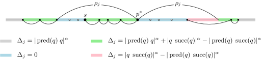
Figure 2: Various cases that can arise when a new point $q$ is inserted into $P$. Open disks indicate zero-range points. The arcs indicate the ranges of the points before the insertion of $q$, where the range of the root-crossing point is drawn both to its right and to its left. The colored intervals relate the possible locations of $q$ to the corresponding values $\Delta_{j}$.

As can be seen in the figure, there are only four possible values for $\Delta_{j}$. This allows us to design our data structure $\mathcal{T}_{p^{*}}$ such that it can be updated using $O(1)$ bulk updates of the following form:

Given an interval $I$ of range values and an update value $\Delta$, add $\Delta$ to the cost of $\Gamma(P,p^{*},\lambda_{j})$ for all $\lambda_{j}\in I$.

In Appendix A we define the information stored in $\mathcal{T}_{p^{*}}$ and we show how bulk updates can be done in $O(\log n)$ time. We eventually obtain the following theorem.

Theorem 2.2.

An optimal solution to the broadcast range-assignment problem for a point set $P$ in $\mathbb{R}^{1}$ can be maintained in $O(n\log n)$ per insertion and deletion, where $n$ is the number of points in the current set $P$.

3 A stable approximation scheme in $\mathbb{R}^{1}$

In this section we use the structure of an optimal solution provided by Theorem 2.1 to obtain a SAS for the 1-dimensional broadcast range-assignment problem. Our SAS has stability parameter $k(\varepsilon)=O((1/\varepsilon)^{1/(\alpha-1)})$, which we will show to be asymptotically optimal.

The optimal range assignment can be very unstable. Indeed, suppose the current point set is $P:=\{s,r_{1},\ldots,r_{n}\}$ with $s=0$ and $r_{i}=i$ ($1\leqslant i\leqslant n$), and take any $\alpha>1$. Then the (unique) optimal assignment $\rho_{\mathrm{opt}}$ has $\rho_{\mathrm{opt}}(s)=\rho_{\mathrm{opt}}(r_{1})=\cdots=\rho_{\mathrm{opt}}(r_{n-1})=1$ and $\rho_{\mathrm{opt}}(r_{n})=0$. If now the point $\ell_{1}=-n$ is inserted, then the optimal assignment becomes $\rho_{\mathrm{opt}}(s)=n$ and $\rho_{\mathrm{opt}}(r_{1})=\cdots=\rho_{\mathrm{opt}}(r_{n})=\rho_{\mathrm{opt}}(\ell_{1})=0$, causing $n$ ranges to be modified.

Next, we will define a feasible solution, referred to as a canonical range assignment $\rho_{k}$ that is more stable than an optimal assignment, while still having a cost close to the cost of an optimal solution. Here $k$ is a parameter that allows a trade-off between stability and quality of the solution. The assignment $\rho_{k}$ for a given point set $P$ will be uniquely determined by the set $P$–it does not depend on the order in which the points have been inserted or deleted. This means that the update algorithm simply works as follows. Let $\rho_{k}(P)$ be the canonical range assignment for a point set $P$, and suppose we update $P$ by inserting a point $q$. Then the update algorithm computes $\rho_{k}(P\cup\{q\})$ and it modifies the range of each point $p\in P\cup\{q\}$ whose canonical range in $\rho_{k}(P\cup\{q\})$ is different from its canonical range in $\rho_{k}(P)$. The goal is now to specify $\rho_{k}$ such that (i) many ranges in $\rho_{k}(P\cup\{q\})$ are the same as in $\rho_{k}(P)$, (ii) the cost of $\rho_{k}(P)$ is close to the cost of $\rho_{\mathrm{opt}}(P)$.

The instance in the example above shows that there can be many points whose range changes from being standard to being zero (or vice versa) when preserving optimality of the consecutive instances. Our idea is therefore to construct solutions where the number of points with zero range is limited, and instead give many points their standard range; if we do this for points whose standard range is relatively small, then the cost of this solution remains bounded compared to the cost of an optimum solution. We now make this idea precise.

Consider a point set $P$ and let $\rho_{\mathrm{opt}}$ be an optimal range assignment satisfying the structure described in Theorem 2.1. Assuming there are points in $P$ on both sides of the source, $\rho_{\mathrm{opt}}$ induces a broadcast tree $\mathcal{B}$ with the structure depicted in Figure 1. Let $\rho_{\mathrm{st}}(p)$ be the standard range of a point $p$. The canonical range assignment $\rho_{k}$ is now defined as follows.

• If all points from $P$ lie to the same side of $s$, then $\rho_{k}(p):=\rho_{\mathrm{opt}}(p)$ for all $p\in P$. Note that in this case $\rho_{k}(p)=\rho_{\mathrm{st}}(p)$ for all $p\in P$.

• Otherwise, let $Z$ be the set of zero-range points in $\rho_{\mathrm{opt}}(P)$. If $|Z|\leqslant k$ then let $Z_{k}:=Z$; otherwise let $Z_{k}\subseteq Z$ be the $k$ points from $Z$ with the largest standard ranges, with ties broken arbitrarily. We define $\rho_{k}$ as follows.

  • $\rho_{k}(p):=\rho_{\mathrm{opt}}(p)$ for all $p\in P\setminus Z$. Observe that this means that $\rho_{k}(p)=\rho_{\mathrm{st}}(p)$ for all $p\in P\setminus Z$ except (possibly) for the root-crossing point.

  • $\rho_{k}(p):=0$ for all $p\in Z_{k}$.

  • $\rho_{k}(p):=\rho_{\mathrm{st}}(p)$ for all $p\in Z\setminus Z_{k}$.

Notice that $\rho_{k}$ is a feasible solution since $\rho_{k}(p)\geqslant\rho_{\mathrm{opt}}(p)$ for each $p\in P$. The next lemma analyzes the stability of the canonical range assignment $\rho_{k}$. Recall that for any range assignment $\rho$—hence, also for $\rho_{k}$—and any point $q$ not in the current set $P$, we have $\rho(q)=0$ by definition. The proof of the following lemma is in the appendix.

Lemma 3.1.

Consider a point set $P$ and a point $q\not\in P$. Let $\rho_{\mathrm{old}}(p)$ be the range of a point $p$ in $\rho_{k}(P)$ and let $\rho_{\mathrm{new}}(p)$ be the range of $p$ in $\rho_{k}(P\cup\{q\})$. Then

$$\left|\{p\in P\cup\{q\}:\rho_{\mathrm{new}}(p)>\rho_{\mathrm{old}}(p)\}\right|\leqslant k+3\mbox{ and }\left|\{p\in P\cup\{q\}:\rho_{\mathrm{new}}(p)<\rho_{\mathrm{old}}(p)\}\right|\leqslant k+3.$$

Next we bound the approximation ratio of $\rho_{k}$.

Lemma 3.2.

For any set $P$ and any $\alpha>1$, we have $\operatorname{cost}_{\alpha}(\rho_{k}(P))\leqslant\left(1+\frac{2^{\alpha}}{k^{\alpha-1}}\right)\cdot\operatorname{cost}_{\alpha}(\rho_{\mathrm{opt}}(P))$.

Proof 3.3.

If all points in $P$ lie to the same side of $s$ then $\rho_{k}(P)=\rho_{\mathrm{opt}}(P)$, and we are done. Otherwise, let $p^{*}$ be the root-crossing point. The only points receiving a different range in $\rho_{k}(P)$ when compared to $\rho_{\mathrm{opt}}(P)$ are the points in $Z\setminus Z_{k}$; these points have $\rho_{k}(p)=\rho_{\mathrm{st}}(p)$ while $\rho_{\mathrm{opt}}(p)=0$. This means we are done when $Z\setminus Z_{k}=\emptyset$. Thus we can assume that $|Z|>k$, so $Z\setminus Z_{k}\neq\emptyset$. Assume without loss of generality that $\rho_{\mathrm{opt}}(p^{*})=1$. As each $p\in Z$ is within reach of $p^{*}$, we have $\sum_{p\in Z}\rho_{\mathrm{st}}(p)\leqslant 2$. Since $Z_{k}$ contains the $k$ points with the largest standard ranges among the points in $Z$, we have $\max\{\rho_{\mathrm{st}}(p):p\in Z\setminus Z_{k}\}\leqslant 2/k$. Hence,

$$\sum_{p\in Z\setminus Z_{k}}\rho_{k}(p)^{\alpha}=\sum_{p\in Z\setminus Z_{k}}\rho_{\mathrm{st}}(p)^{\alpha}=\sum_{p\in Z\setminus Z_{k}}\rho_{\mathrm{st}}(p)^{\alpha-1}\cdot\rho_{\mathrm{st}}(p)\leqslant\left(\frac{2}{k}\right)^{\alpha-1}\sum_{p\in Z\setminus Z_{k}}\rho_{\mathrm{st}}(p)\leqslant\frac{2^{\alpha}}{k^{\alpha-1}}.$$

(The analysis can be made tighter by using that $\sum_{p\in Z\setminus Z_{k}}\rho_{\mathrm{st}}(p)\leqslant 2-k\max_{p\in Z\setminus Z_{k}}\rho_{\mathrm{st}}(p)$, but this will not change the approximation ratio asymptotically.) We conclude that

$$\frac{\operatorname{cost}_{\alpha}(\rho_{k}(P))}{\operatorname{cost}_{\alpha}(\rho_{\mathrm{opt}}(P))}\leqslant\frac{\sum_{p\in P\setminus(Z\setminus Z_{k})}\rho_{k}(p)^{\alpha}+\sum_{p\in Z\setminus Z_{k}}\rho_{k}(p)^{\alpha}}{\sum_{p\in P\setminus(Z\setminus Z_{k})}\rho_{\mathrm{opt}}(p)^{\alpha}}\leqslant 1+\frac{2^{\alpha}}{k^{\alpha-1}},$$

where the last inequality follows because we have $\rho_{k}(p)=\rho_{\mathrm{opt}}(p)$ for all $p\in P\setminus(Z\setminus Z_{k})$ and $\sum_{p\in P\setminus(Z\setminus Z_{k})}\rho_{\mathrm{opt}}(p)^{\alpha}\geqslant 1$.

By maintaining the canonical range assignment $\rho_{k}$ for $k=(2^{\alpha}/\varepsilon)^{1/(\alpha-1)}=O((1/\varepsilon)^{1/(\alpha-1)})$ we obtain the following theorem.

Theorem 3.4.

There is a SAS for the dynamic broadcast range-assignment problem in $\mathbb{R}^{1}$ with stability parameter $k(\varepsilon)=O((1/\varepsilon)^{1/(\alpha-1)})$, where $\alpha>1$ is the distance-power gradient. The time needed by the SAS to compute the new range assignment upon the insertion or deletion of a point is $O(n\log n)$, where $n$ is the number of points in the current set.

Next we show that the stability parameter $k(\varepsilon)$ in our SAS is asymptotically optimal.

Theorem 3.5.

Any SAS for the dynamic broadcast range-assignment problem in $\mathbb{R}^{1}$ must have stability parameter $k(\varepsilon)=\Omega((1/\varepsilon)^{1/(\alpha-1)})$, where $\alpha>1$ is the distance-power gradient.

Proof 3.6.

Let

4 The problem in $\mathbb{S}^{1}$

We now turn to the setting where the underlying space is $\mathbb{S}^{1}$, that is, the points in $P$ lie on a circle and distances are measured along the circle. In Section 4.1, we prove that the structure of an optimal solution in $\mathbb{S}^{1}$ is very similar to the structure of an optimal solution in $\mathbb{R}^{1}$ as formulated in Theorem 2.1. In spite of this, and contrary to the problem in $\mathbb{R}^{1}$, we prove in Section 4.2 that no SAS exists for the problem in $\mathbb{S}^{1}$.

Again, we denote the source point by $s$. The clockwise distance from a point $p\in\mathbb{S}^{1}$ to a point $q\in\mathbb{S}^{1}$ is denoted by $d_{\mathrm{cw}}(p,q)$, and the counterclockwise distance by $d_{\mathrm{ccw}}(p,q)$. The actual distance is then $d(p,q):=\min(d_{\mathrm{cw}}(p,q),d_{\mathrm{ccw}}(p,q))$. The closed and open clockwise interval from $p$ to $q$ are denoted by $[p,q]^{\mathrm{cw}}$ and $(p,q)^{\mathrm{cw}}$, respectively.

4.1 The structure of an optimal solution in $\mathbb{S}^{1}$

Here we prove that the structure of an optimal solution in $\mathbb{S}^{1}$ is very similar to the structure of an optimal solution in $\mathbb{R}^{1}$. The heart of this proof is the following lemma, whose (rather intricate) proof is given in Appendix LABEL:app:structure-in-S1. Define the covered region of $P$ with respect to a range assignment $\rho$, denoted by $\mathrm{cov}(\rho,P)$, to be the set of all points $r\in\mathbb{S}^{1}$ such that there exists a point $p\in P$ with $\rho(p)\geqslant d(p,r)$.

Lemma 4.1.

Let $P$ be a point set in $\mathbb{S}^{1}$ with $|P|>2$ and let $\rho_{\mathrm{opt}}$ be an optimal range assignment for $P$. Then there exists a point $r\in\mathbb{S}^{1}$ such that $r\notin\mathrm{cov}(\rho_{\mathrm{opt}},P)$.

Lemma 4.1 implies that an optimal solution for an instance in $\mathbb{S}^{1}$ corresponds to an optimal solution for an instance in $\mathbb{R}^{1}$ derived as follows. For a point $r\in\mathbb{S}^{1}$, define the mapping $\mu_{r}:P\rightarrow\mathbb{R}^{1}$ such that $\mu_{r}(s):=0$, and $\mu_{r}(p):=d_{\mathrm{cw}}(s,p)$ for all $p\in[s,r]^{\mathrm{cw}}$, and $\mu_{r}(p):=-d_{\mathrm{ccw}}(s,p)$ for all $p\in[r,s]^{\mathrm{cw}}$. Let $\mu_{r}(P)$ denote the resulting point set in $\mathbb{R}^{1}$.

Theorem 4.2.

Let $P$ be an instance of the broadcast range-assignment problem in $\mathbb{S}^{1}$. There exists a point $r\in\mathbb{S}^{1}$ such that an optimal range assignment for $\mu_{r}(P)$ in $\mathbb{R}^{1}$ induces an optimal range assignment for $P$. Moreover, we can compute an optimal range assignment for $P$ in $O(n^{2}\log n)$ time, where $n$ is the number of points in $P$.

Proof 4.3.

Let $r\in\mathbb{S}^{1}$ be a point such that $r\notin\mathrm{cov}(\rho_{\mathrm{opt}},P)$, which exists by Lemma 4.1. Consider the mapping $\mu_{r}$. Any feasible range assignment for $\mu_{r}(P)$ induces a feasible range assignment for $P$ in $\mathbb{S}^{1}$, since $d(p,q)\leqslant|\mu_{r}(p)\mu_{r}(q)|$ for any two points $p,q\in P$. Conversely, an optimal range assignment for $P$ induces a feasible range assignment for $\mu_{r}(P)$, since the point $r$ is not covered in the optimal solution. This proves the first part of the theorem.

Now let $P:=\{s,p_{1},\ldots,p_{n}\}$, where the points $p_{i}$ are ordered clockwise from $s$. For $0\leqslant i\leqslant n$, let $r_{i}$ be a point in $(p_{i},p_{i+1})^{\mathrm{cw}}$, where $p_{0}=p_{n+1}=s$. Since $\mu_{r_{i}}=\mu_{r}$ for any $r\in(p_{i},p_{i+1})^{\mathrm{cw}}$, an optimal solution can be computed by finding the best solution over all mappings $\mu_{r_{i}}$. The only difference between $\mu_{r_{i}}$ and $\mu_{r_{i+1}}$ is the location that $p_{i+1}$ is mapped to, so after computing an optimal solution for $\mu_{1}(P)$ in $O(n^{2}\log n)$ time, we can go through the mappings $\mu_{2},\ldots,\mu_{n}$ and update the optimal solution in $O(n\log n)$ time using Theorem 2.2. Hence, an optimal range assignment for $P$ can be computed in $O(n^{2}\log n)$ time.

4.2 Non-existence of a SAS in $\mathbb{S}^{1}$

We have seen that an optimal solution for a set $P$ in $\mathbb{S}^{1}$ can be obtained from an optimal solution in $\mathbb{R}^{1}$, if we cut $\mathbb{S}^{1}$ at an appropriate point $r$. It is a fact however that the insertion of a new point into $P$ may cause the location of the cutting point $r$ to change drastically. Next we show that this means that the dynamic problem in $\mathbb{S}^{1}$ does not admit a SAS.

Theorem 4.4.

The dynamic broadcast range-assignment problem in $\mathbb{S}^{1}$ with distance power gradient $\alpha>1$ does not admit a SAS. In particular, there is a constant $c_{\alpha}>1$ such that the following holds: for any $n$ large enough, there is a set $P:=\{s,p_{1},\ldots,p_{2n+1}\}$ and a point $q$ in $\mathbb{S}^{1}$ such that any update algorithm

The rest of this section is dedicated to proving Theorem 4.4. We will prove the theorem for

$$c_{\alpha}:=\min\left(1+2^{\alpha-4}-\frac{1}{8},\ 1+\frac{2^{\alpha-1}-1}{3\cdot 2^{\alpha}+2},\ 1+\frac{\min\left(2^{\alpha}-1,\frac{3^{\alpha}-2^{\alpha}-1}{2},\frac{4^{\alpha}-2^{\alpha}-2}{3}\right)}{4(2^{\alpha}+1)}\right).$$

Note that each term is a constant strictly greater than 1 for any fixed constant $\alpha>1$. In particular, for $\alpha=2$ we have $c_{\alpha}=1+\frac{1}{14}$.

Let $P:=\{s,p_{1},\ldots,p_{2n+1}\}$, where $d_{\mathrm{cw}}(p_{i},p_{i+1})=2$ for odd $i$ and $d_{\mathrm{cw}}(p_{i},p_{i+1})=1$ for even $i$; see Fig. 3(i). Let $d_{\mathrm{cw}}(s,p_{1})=\delta$, where $\delta^{\alpha}=(2^{\alpha}+1)n$. Finally, let $d_{\mathrm{cw}}(p_{2n+1},q)=d_{\mathrm{cw}}(q,s)=x\delta$, where $x^{\alpha}=\frac{1}{4}+\left(\frac{1}{2}\right)^{\alpha+1}$. Note that $(1/2)^{\alpha}<x^{\alpha}<1/2$ for any $\alpha>1$.

Figure 3: (i) The instance showing that there is no SAS in $\mathbb{S}^{1}$. (ii) The instance in $\mathbb{R}^{2}$.

Let $\rho(p)$ denote the range given to a point $p$ by

Algorithm 9.

. A directed edge $(p,p^{\prime})$ in the communication graph induced by $\rho$ is called a clockwise edge if $\rho(p)\geqslant d_{\mathrm{cw}}(p,p^{\prime})$, and it is called a counterclockwise edge if $\rho(p)\geqslant d_{\mathrm{ccw}}(p,p^{\prime})$. Observe that we may assume that no edge $(p,p^{\prime})$ is both clockwise and counterclockwise, because otherwise $\rho(p)\geqslant(\delta+3n+2x\delta)/2$, which is much too expensive for an approximation ratio of at most $c_{\alpha}$. Define the range $\rho(p)$ of a point in $P$ to be cw-minimal if $\rho(p)$ equals the distance from $p$ to its clockwise neighbor in $P$. Similarly, $\rho(p)$ is ccw-minimal if $\rho(p)$ equals the distance from $p$ to its counterclockwise neighbor. The idea of the proof is to show that before the insertion of $q$, most of the points $s,p_{1},\ldots,p_{2n+1}$ must have a cw-minimal range, while after the insertion most points must have a ccw-minimal range. This will imply that many ranges must be modified from being cw-minimal to being ccw-minimal.

Before the insertion of $q$, giving every point a cw-minimal range leads to a feasible assignment of total cost $\delta^{\alpha}+(2^{\alpha}+1)n=2\delta^{\alpha}$. After the insertion of $q$, giving every point a ccw-minimal range leads to a feasible assignment of total cost $2(x\delta)^{\alpha}+(2^{\alpha}+1)n=(2x^{\alpha}+1)\delta^{\alpha}$. Hence, if $\mbox{{\sc opt}}(\cdot)$ denotes the cost of an optimal range assignment, then we have: $\mbox{{\sc opt}}(P)\leqslant 2\delta^{\alpha}$   and   $\mbox{{\sc opt}}(P\cup\{q\})\leqslant(2x^{\alpha}+1)\delta^{\alpha}<2\delta^{\alpha}$. We first prove a lower bound on the total cost of the points $p_{1},\ldots,p_{2n+1}$. Intuitively, only $o(n)$ of those points can be reached from $s$ or $q$ (otherwise the range of $s$ or $q$ would be too expensive) and the cheapest way to reach the remaining points will be to use only cw-minimal or ccw-minimal ranges. A formal proof of the lemma is given in Appendix LABEL:app:no-sas-missing-proofs.

Lemma 4.5.

$\sum_{i=1}^{2n+1}\rho(p_{i})^{\alpha}\geqslant(2^{\alpha}+1)n-o(n)$, both before and after the insertion of $q$.

The following lemma gives a key property of the construction.

Lemma 4.6.

The point $p_{2n+1}$ cannot have an incoming counterclockwise edge before $q$ is inserted, and the point $p_{1}$ cannot have an incoming clockwise edge after $q$ has been inserted.

Proof 4.7.

The cheapest incoming counterclockwise edge for $p_{2n+1}$ before the insertion of $q$ is from $s$, but this is too expensive for

We are now ready to prove that many edges must change from being cw-minimal to being ccw-minimal when $q$ is inserted.

Lemma 4.8.

Before the insertion of $q$, at least $4n/3+1$ of the points from $\{s,p_{1},\ldots,p_{2n}\}$ have a cw-minimal range and after the insertion of $q$ at least $4n/3+1$ of the points from $\{q,p_{1},\ldots,p_{2n}\}$ have a ccw-minimal range.

Proof 4.9.

We prove the lemma for the situation before $q$ is inserted; the proof for the situation after the insertion of $q$ is similar. Observe that before and after the insertion of $q$, the distance between any two points is either 1, 2 or at least 3. Hence, in what follows we may assume that $\rho(p)\in\{0,1,2\}\cup[3,\infty)$ for any point $p\in P\cup\{q\}$.

It will be convenient to define $p_{0}:=s$ (although we may still use $s$ if we want to stress that we are talking about the source). Recall that $p_{2n+1}$ does not have an incoming counterclockwise edge in the communication graph $\mathcal{G}_{\rho}(P)$ before the insertion of $q$. Let $\pi^{*}$ be a minimum-hop path from $s$ to $p_{2n+1}$ in $\mathcal{G}_{\rho}(P)$. Since $p_{2n+1}$ does not have an incoming counterclockwise edge and $\pi^{*}$ is a minimum-hop path, all edges in $\pi$ are clockwise. We assign each point $p_{j}$ with $1\leqslant j\leqslant 2n+1$ to the edge $(p_{i},p_{t})$ in $\pi^{*}$ such that $i+1\leqslant j\leqslant t$, and we define $A(p_{i},p_{t}):=\{p_{i+1},\ldots,p_{t}\}$ to be the set of all points assigned to $(p_{i},p_{t})$. We define the excess of a point $p_{j}\in A(p_{i},p_{t})$ to be

$$\mathrm{excess}(p_{j}):=\frac{1}{|A(p_{i},p_{t})|}\cdot\left(\rho(p_{i})^{\alpha}-\sum_{p_{\ell}\in A(p_{i},p_{t})}d(p_{\ell-1},p_{\ell})^{\alpha}\right).$$

We say that an edge $(p_{i},p_{t})$ in $\pi^{*}$ is cw-minimal if $p_{i}$ has a cw-minimal range. Note that if a point $p_{j}$ is assigned to a cw-minimal edge, then this is the edge $(p_{j-1},p_{j})$ and $\mathrm{excess}(p_{j})=0$. Intuitively, $\mathrm{excess}(p_{j})$ denotes the additional cost we pay for reaching $p_{j}$ compared to reaching it by a cw-minimal edge, if we distribute the additional cost of a non-cw-minimal edge over the points assigned to it. Because each of the points $p_{1},\ldots,p_{2n+1}$ is assigned to exactly one edge on the path $\pi^{*}$, we have

$$\sum_{p_{i}\in\pi^{*}}\rho(p)^{\alpha}\geqslant\sum_{j=1}^{2n+1}d(p_{j-1},p_{j})^{\alpha}+\sum_{j=1}^{2n+1}\mathrm{excess}(p_{j})\geqslant\mbox{{\sc opt}}(P)+\sum_{j=1}^{2n+1}\mathrm{excess}(p_{j})$$ (1)

where the second inequality follows from Observation 9 and because $p_{0}=s$. The following claim is proved in Appendix LABEL:app:no-sas-missing-proofs. (Essentially, the smallest possible excess is obtained when $|A(p_{i},p_{t})|\in\{1,2,3\}$; the three terms in the claim correspond to these cases.)

• Claim. If $p_{j}$ is not assigned to a cw-minimal edge then $\mathrm{excess}(p_{j})\geqslant c^{\prime}_{\alpha}$, where $c^{\prime}_{\alpha}=\min\left(2^{\alpha}-1,\frac{3^{\alpha}-2^{\alpha}-1}{2},\frac{4^{\alpha}-2^{\alpha}-2}{3}\right)$.

Now suppose for a contradiction that less than $4n/3+1$ points from $\{s,p_{1},\ldots,p_{2n+1}\}$ have a cw-minimal range. Then at least $2n/3+1$ points $p_{j}$ have $\mathrm{excess}(p_{j})\geqslant c^{\prime}_{\alpha}$ by the claim above. By Inequality (1) the total cost incurred by

Lemma 4.8 implies that at least $4n/3$ of the points $p_{1},\ldots,p_{2n+1}$ have a cw-minimal range before $q$ is inserted, and at least $4n/3$ of those points have a ccw-minimal range after the insertion. Hence, at least $2n+1-2\cdot(2n/3+1)=2n/3-1$ points must change from being cw-minimal to being ccw-minimal, thus finishing the proof of Theorem 4.4.

5 The 2-dimensional problem

The broadcast range-assignment problem is np-hard in $\mathbb{R}^{2}$, so we cannot expect a characterization of the structure of an optimal solution similar to Theorem 2.1. Using a similar construction as in $\mathbb{S}^{1}$ we can also show that the problem in $\mathbb{R}^{2}$ does not admit a SAS.

Theorem 5.1.

The dynamic broadcast range-assignment problem in $\mathbb{R}^{2}$ with distance power gradient $\alpha>1$ does not admit a SAS. In particular, there is a constant $c_{\alpha}>1$ such that the following holds: for any $n$ large enough, there is a set $P:=\{s,p_{1},\ldots,p_{2n+1}\}$ and a point $q$ in $\mathbb{R}^{2}$ such that any update algorithm

Proof 5.2.

We use the same construction as in $\mathbb{S}^{1}$, where we embed the points on a square and the distances used to define the instance are measured along the square; see Fig. 3(ii). For any two points on the same edge of the square, their distance along the square is the same as their distance in $\mathbb{R}^{2}$. Moreover, we know that no range can be larger than $3\delta$, otherwise the range assignment is already too expensive. Note that the number of points $p_{i}$ within distance $3\delta$ from a corner is $o(n)$. Using this fact we can argue that all lemmas from Section 4.2 still hold. (For example, in the proof of Lemma 4.8 we can simply ignore the excess of $o(n)$ points.) This is argued more extensively in Appendix LABEL:app:no-SAS-R2.

Although the problem in $\mathbb{R}^{2}$ does not admit a SAS, there is a relatively simple $O(1)$-stable $O(1)$-approximation algorithm for $\alpha\geqslant 2$. The algorithm is based on a result by Ambühl [1], who showed that a minimum spanning tree (MST) on $P$ gives a 6-approximation for the static broadcast range-assignment problem: turn the MST into a directed tree rooted at the source $s$, and assign as a range to each point $p\in P$ the maximum length of any of its outgoing edges. To make this solution stable, we set the range of each point to the maximum length of any of its incident edges (not just the outgoing ones). Because an MST in $\mathbb{R}^{2}$ has maximum degree 6, this leads to 17-stable 12-approximation algorithm; see Appendix LABEL:app:mst-in-R2.

6 Concluding remarks

We studied the dynamic broadcast range-assignment problem from a stability perspective, introducing the notions of $k$-stable algorithms and stable approximation schemes (SASs). Our results provide a fairly complete picture of the problem in $\mathbb{R}^{1}$, in $\mathbb{S}^{1}$, and in $\mathbb{R}^{2}$. In particular, we presented a SAS in $\mathbb{R}^{1}$ that has an asymptotically optimal stability parameter, and showed that the problem does not admit a SAS in $\mathbb{S}^{1}$ and $\mathbb{R}^{2}$. Future work can focus on improving (the upper and/or lower bounds for) the approximation ratios we have obtained for algorithms with constant stability parameter. In particular, it is open whether there exists a 2-stable algorithm with approximation ratio less than 2 in $\mathbb{R}^{1}$. It would also be interesting to use develop algorithm with small stability parameter in $\mathbb{S}^{1}$, possibly using the relation we proved between the structure of an optimal structure in in $\mathbb{S}^{1}$ and in $\mathbb{R}^{1}$.

Appendix A A data structure for maintaining an optimal solution

Below we give a detailed description of the data structure to maintain an optimal solution in $\mathbb{R}^{1}$. For convenience, we repeat somematerial from the main text, so that the description below is self-contained.

Recall that an optimal solution for a given point set $P$ has a single root-crossing point, $p^{*}$. Once the range of $p^{*}$ is fixed, the solution is completely determined. The range of $p^{*}$ is defined by some other point from $P$—we have $\rho(p^{*})=|p^{*}p|$ for some point $p\neq p^{*}$—and so there are $n-1$ candidate ranges for a given choice of the root-crossing point $p^{*}$. The idea of our solution is to implicitly store the cost of the range assignment for each candidate range of $p^{*}$ such that, upon the insertion or deletion of a point in $P$, we can in $O(\log n)$ time find the best range for $p^{*}$. By maintaining $n$ such data structures $\mathcal{T}_{p^{*}}$, one for each choice of the root-crossing point $p^{*}$, we can then find the overall best solution.

Besides the data structures $\mathcal{T}_{p^{*}}$ which are described below, we also maintain a global data structure $\mathcal{T}_{P}$ that supports the following operations.

• Find the predecessor $\operatorname{pred}(q)$ and successor $\operatorname{succ}(q)$ in $P$ of a query point $q$.

• Given two points $p,p^{\prime}\in P$, report the total cost of the chain from $p$ to $p^{\prime}$.

• Insert or delete points from $P$.

By implementing $\mathcal{T}_{P}$ as a suitably augmented binary search tree—see the book by Cormen et al. [15, Chapter 15] for the design and maintenance of such structures—each of these operations can be performed in $O(\log n)$ time.

The data structure for a given root-crossing point. Next we explain our data structure for a given candidate root-crossing point $p^{*}$. We assume without loss of generality that $p^{*}$ lies to the right of the source point $s$; it is straightforward to adapt the structure to the (symmetric) case where $p^{*}$ lies to the left of $s$, and to the case where $p^{*}=s$.

Let $\mathcal{R}_{p^{*}}$ be the set of all ranges we need to consider for $p^{*}$, for the current set $P$. The range of a root-crossing point must extend beyond the source point. Hence,

$$\mathcal{R}_{p^{*}}:=\{|p^{*}p|:p\in P\mbox{ and }|p^{*}p|>|p^{*}s|\}.$$

Let $\lambda_{1},\ldots,\lambda_{m}$ denote the sequence of ranges in $\mathcal{R}_{p^{*}}$, ordered from small to large. (If $\mathcal{R}_{p^{*}}=\emptyset$, there is nothing to do and our data structure is empty.) As mentioned, once we fix a range $\lambda_{j}$ for the given root-crossing point $p^{*}$, the solution is fully determined by Theorem 2.1: there is a chain from $s$ to $p^{*}$, a chain from the rightmost point within range of $p^{*}$ to the right-extreme point, and a chain from the leftmost point within range of $p^{*}$ to the left-extreme point. We denote the resulting range assignment for $P$ by $\Gamma(P,p^{*},\lambda_{j})$.

There is one subtlety in the definition of $\Gamma(P,p^{*},\lambda_{j})$, namely when there are no points within reach of $p^{*}$ to, say, the right of $p^{*}$; see Figure 4. Such a solution can never be optimal, but we must maintain it nevertheless, because the range $\lambda_{j}$ may become relevant later. To deal with this situation, we will insert a dummy point whose location coincides with $p^{*}$ and that is defined to be the predecessor of $\operatorname{succ}(p^{*})$. Note that the dummy will become a zero-range point as soon as an actual point is inserted that is within the range of $p^{*}$ and lies to the same side of $p^{*}$ as the dummy.

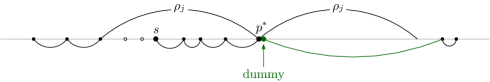
Figure 4: A dummy point is inserted to ensure that points to the right of $p^{*}$ can be reached. For clarity the dummy is drawn to the right of $p^{*}$, but it actually coincides with $p^{*}$.

Our data structure, which implicitly stores the costs of the range assignments $\Gamma(P,p^{*},\lambda_{j})$ for all $\lambda_{j}\in\mathcal{R}_{p^{*}}$, is an augmented balanced binary search tree $\mathcal{T}_{p^{*}}$, defined as follows.

• The leaves of $\mathcal{T}_{p^{*}}$ are in one-to-one correspondence with the candidate ranges in $\mathcal{R}_{p^{*}}$: the leftmost leaf corresponds to $\lambda_{1}$, the next left to $\lambda_{2}$, and so on. From now on, with a slight abuse of notation, we use $\lambda_{j}$ to refer to a range in $\mathcal{R}_{p^{*}}$ as well as to the corresponding leaf.

• Each leaf stores, besides the corresponding range $\lambda_{j}$, a value $f(\lambda_{j})$. Initially $f(\lambda_{j})$ will be equal to the cost of $\Gamma(P,p^{*},\lambda_{j})$. Later this may no longer be the case, however.

• The internal nodes of $\mathcal{T}_{p^{*}}$ are augmented with extra information, as follows. For an internal node $v$, let $\mathcal{R}_{p^{*}}(v)\subseteq\mathcal{R}_{p^{*}}$ be the set of all ranges stored in the leaves of the subtree rooted at $v$. The node $v$ stores the following additional information, besides the splitting values that we have because $\mathcal{T}_{p^{*}}$ is a search tree on the ranges in $\mathcal{R}_{p^{*}}$:

  • A correction value $\Delta(v)\in\mathbb{R}$.

  • A value $\operatorname{min-cost}(v)$ defined as follows. For a range $\lambda_{j}\in\mathcal{R}_{p^{*}}(v)$ define the local cost of $\lambda_{j}$ at $v$ to be $f(\lambda_{j})+\sum_{u}\Delta(u)$, where the sum is over all nodes $u$ on the path from $v$ (and including $v$) to $\lambda_{j}$. Then $\operatorname{min-cost}(v)$ is defined to be the minimum local cost over all ranges in $\mathcal{R}_{p^{*}}(v)$.

  • A range $\lambda_{j}\in\mathcal{R}_{p^{*}}(v)$ whose local cost at $v$ is $\operatorname{min-cost}(v)$. This range is denoted by $\operatorname{best-range}(v)$.

Our update algorithm will ensure the following invariant:

For any range $$\lambda_{j}\in\mathcal{R}_{p^{*}} \Gamma(P,p^{*},\lambda_{j}) f(\lambda_{j})+\sum_{u}\Delta(u) \operatorname{root}(\mathcal{T}_{p^{*}}) \lambda_{j}$$, the total cost of is equal to , where the sum is over all nodes on the search path from to . (5)

In other words, Invariant (5) states that, for any range $\lambda_{j}$, the local cost of $\lambda_{j}$ at the root of $\mathcal{T}_{p^{*}}$ is equal to the actual cost of $\Gamma(P,p^{*},\lambda_{j})$. Since $\mathcal{R}_{p^{*}}(\operatorname{root}(\mathcal{T}_{p^{*}}))=\mathcal{R}_{p^{*}}$, this implies that $\operatorname{min-cost}(\operatorname{root}(\mathcal{T}_{p^{*}}))$ equals the minimum cost that can be obtained by a solution that uses $p^{*}$ as a root-crossing point.

Updating the data structure. We now describe how to update the structure upon the insertion of a new point. Deletions can be handled in a symmetrical manner. To simplify the presentation, we assume that no two points in $P$ coincide; the solution is easily adapted to the case where $P$ can be a multi-set.

Figure 5: Various cases that can arise when a new point $q$ is inserted into $P$. Open disks indicate zero-range points. The arcs indicate the ranges of the points before the insertion of $q$, where the range of the root-crossing point is drawn both to its right and to its left. The colored intervals relate the possible locations of $q$ to the corresponding values $\Delta_{j}$.

Let $\Delta_{j}$ be the (signed) difference of the cost of the range assignment $\Gamma(P,p^{*},\lambda_{j})$ before and after the insertion of $q$, where $\Delta_{j}$ is positive if the cost increases. Figure 5 shows various possible values for $\Delta_{j}$, depending on the location of the new point $q$. The figure is for the generic case, when $Z_{\mathrm{left}},Z_{\mathrm{right}}\neq\emptyset$ and there are points to the right as well as to the left of the interval that is within reach of the root-crossing point $p^{*}$. Lemma A.1, which is easy to verify, gives the values for $\Delta_{j}$ for all cases, where we write $p<q$ when a point $p$ is to the left of a point $q$.

Lemma A.1.

Let $\Delta_{j}:=\operatorname{cost}\left(\Gamma(P\cup\{q\},p^{*},\lambda_{j})\right)-\left(\Gamma(P,p^{*},\lambda_{j})\right)$. If $s<q<p^{*}$ or $p^{*}<q<s$ we have

$$\Delta_{j}=|\operatorname{pred}(q)\;q|^{\alpha}+|q\;\operatorname{succ}(q)|^{\alpha}-|\operatorname{pred}(q)\;\operatorname{succ}(q)|^{\alpha}$$

Otherwise we have

$$\Delta_{j}=\left\{\begin{array}[]{ll}|q\;\operatorname{succ}(q)|^{\alpha}-|\operatorname{pred}(q)\;\operatorname{succ}(q)|^{\alpha}&\mbox{if $|p^{*}q|\leqslant\rho_{j}<|p^{*}\;\operatorname{succ}(q)|$}\\[5.69054pt] 0&\mbox{if $\rho_{j}\geqslant|p^{*}\;\operatorname{succ}(q)|$}\\ &\hskip 8.53581pt\mbox{or $\big{(}\lambda_{j}\geqslant|p^{*}q|$ and $\operatorname{succ}(q)=\mbox{\sc nil}\big{)}$}\\[5.69054pt] |\operatorname{pred}(q)\;q|^{\alpha}+|q\;\operatorname{succ}(q)|^{\alpha}-|\operatorname{pred}(q)\;\operatorname{succ}(q)|^{\alpha}&\mbox{if $\lambda_{j}<|p^{*}q|$ and $\operatorname{succ}(q)\neq\mbox{\sc nil}$}\\[5.69054pt] |\operatorname{pred}(q)\;q|^{\alpha}&\mbox{if $\lambda_{j}<|p^{*}q|$ and $\operatorname{succ}(q)=\mbox{\sc nil}$}\end{array}\right.$$

Lemma A.1 implies that, after computing $\operatorname{pred}(q)$ and $\operatorname{succ}(q)$, we can update our data structure using $O(1)$ bulk updates of the following form:

Given an interval $I$ of range values and an update value $\Delta$, add $\Delta$ to the cost of $\Gamma(P,p^{*},\lambda_{j})$ for all $\lambda_{j}\in I$.

We cannot afford to do this explicitly, so we implement bulk updates by updating the auxiliary information stored in $O(\log n)$ nodes in $\mathcal{T}_{p^{*}}$, as follows.

1. Let $\lambda_{\min}$ and $\lambda_{\max}]$ be the two endpoints of the interval $I$ (possibly $\lambda_{\max}]=\infty$). By searching with $\lambda_{\min}$ and $\lambda_{\max}]$ in $\mathcal{T}_{p^{*}}$, identify a collection $\mathcal{C}(I)$ of $O(\log n)$ nodes in $\mathcal{T}_{p^{*}}$ such that $\lambda_{i}\in I$ if and only if the leaf storing $\lambda_{j}$ is a descendant of a node in $\mathcal{C}(I)$.

2. Add $\Delta$ to the correction values $\Delta(v)$ of all nodes $v\in\mathcal{C}(I)$ and to the value $\operatorname{min-cost}(v)$.

3. Update the values $\Delta(v)$, $\operatorname{min-cost}(v)$, and $\operatorname{best-range}(v)$ of the $O(\log n)$ ancestors of the nodes in $\mathcal{C}(v)$ in a bottom-up manner.

Since algorithms for updating this type of auxiliary information are rather standard we omit further details.

Besides updating the costs of the assignments $\Gamma(P,p^{*},\lambda_{j})$, we may also need to introduce another candidate range for $p^{*}$. In particular, we need to introduce the range $|p^{*}q|$ if $|p^{*}q|>|p^{*}s|$. To this end we need to compute the cost of the range assignment $\Gamma(P,p^{*},|p^{*}q|)$. After computing $\operatorname{pred}(q)$, $\operatorname{succ}(q)$, and the cost of $O(1)$ chains—this can all be done in $O(\log n)$ time using the global tree $\mathcal{T}_{P}$—we can compute the cost of $\Gamma(P,p^{*},|p^{*}q|)$ in $O(1)$ time. We then insert a leaf $w$ for the range $|p^{*}q|$ into $\mathcal{T}_{p^{*}}$ with $f(|p^{*}q|)$ equal to the just computed cost. Finally, we update the values $\operatorname{min-cost}(v)$ and $\operatorname{best-range}(v)$ of the ancestors $v$ of $w$ whose the current value of $\operatorname{min-cost}(v)$ is larger than $f(|p^{*}q|)$). (Re-balancing $\mathcal{T}_{p^{*}}$, when necessary, can be done in a standard manner [15, Chapter 15].)

The following lemma summarizes the discussion above.

Lemma A.2.

$\mathcal{T}_{p^{*}}$ can be updated in $O(\log n)$ time per insertion and deletion.

Putting it all together. To summarize, upon the insertion of a new point $q$ into $P$, we first update each tree $\mathcal{T}_{p^{*}}$, as described above. This takes in $O(\log n)$ time per tree, so $O(n\log n)$ time in total. Then we update the global tree $\mathcal{T}_{P}$ in $O(\log n)$ time. Finally, we create a tree $\mathcal{T}_{q}$ with $q$ being the root-crossing point. This can be done in $O(n\log n)$ time, by inserting the points from $P$ one by one as described above. Thus inserting a new point $q$ can be done in $O(n\log n)$ time in total, after which we know the cost of the optimal solution for $P\cup\{q\}$. Deletions can be handled in a similar manner, so we obtain the following theorem. See 2.2

Appendix B Missing proofs for Section 3

B.1 Proof of Lemma 3.1

See 3.1

Proof B.1.

The range of a point $p\in P\cup\{q\}$ can increase due to the insertion of $q$ only if

(i)

$p=q$ and $\rho_{\mathrm{new}}(q)>0$, or

(ii)

$p$ is a zero-range point in $\rho_{k}(P)$, or

(iii)

$p$ is the root-crossing point in $\rho_{k}(P\cup\{q\})$, or

(iv)

the standard range of $p$ increases due to the insertion of $q$, or

(v)

$p=s$ and, out of the two standard ranges it has, $s$ gets assigned a larger one in $\rho_{k}(P\cup\{q\})$ than in $\rho_{k}(P)$.

Recall that we defined $\rho_{k}$ such that the number of zero-range points is at most $k$. Furthermore, at most one standard range can increase due to the insertion of $q$, namely, the standard range of a point that is extreme in $P$ but not in $P\cup\{q\}$. When this happens, however, $q$ is extreme in $P\cup\{q\}$ and so $\rho_{\mathrm{new}}(q)=0$; this implies that cases (i) and (iv) cannot both happen. Hence, $\left|\{p\in P\cup\{q\}:\rho_{\mathrm{new}}(p)>\rho_{\mathrm{old}}(p)\}\right|\leqslant k+3$.

The range of a point $p$ can decrease only if

(i)

$p$ is a zero-range point in $\rho_{k}(P\cup\{q\})$, or

(ii)

$p$ is the root-crossing point in $\rho_{k}(P)$, or

(iii)

the standard range of $p$ decreases due to the insertion of $q$, or

(iv)

$p=s$ and, out of the two standard ranges it has, $p$ gets a assigned a smaller one in $\rho_{k}(P\cup\{q\})$ than in $\rho_{k}(P)$.

Since the only point whose standard range decreases is the predecessor of $q$ in $P$, we conclude that $\left|\{p\in P\cup\{q\}:\rho_{\mathrm{new}}(p)<\rho_{\mathrm{old}}(p)\}\right|\leqslant k+3$.

B.2 Proof of Theorem 3.4

See 3.4

Proof B.2.

Our SAS maintains the canonical range assignment $\rho_{k}$ for $k=(2^{\alpha}/\varepsilon)^{1/(\alpha-1)}=O((1/\varepsilon)^{1/(\alpha-1)})$. We then have $\operatorname{cost}_{\alpha}(\rho_{k}(P))\leqslant(1+\varepsilon)\cdot\rho_{\mathrm{opt}}(P)$ by Lemma 3.2. Furthermore, the number of modified ranges when $P$ is updated is $2k+6$ by Lemma 3.1. To determine the assignment $\rho_{k}$, we need to know an optimal assignment $\rho_{\mathrm{opt}}$ with the structure from Theorem 2.1. Such an optimal assignment can be maintained in $O(n\log n)$ time per update, by Theorem 2.2. Once we have the new optimal assignment, the new optimal assignment can be determined in $O(n)$ time.

Appendix C 1-Stable, 2-Stable, and 3-Stable Algorithms in $\mathbb{R}^{1}$

In Section 3 we presented a $(2k+6)$-stable algorithm whose approximation ratio is $1+2^{\alpha}/k^{\alpha-1}$, which provided us with a SAS. For small $k$ the algorithm is not very good: the most stable algorithm we can get is 6-stable, by setting $k=0$. A more careful analysis shows that the approximation ratio of this 6-stable algorithm is 3, for $\alpha=2$. In this section we study more stable algorithms. We first present a 1-stable $O(1)$-approximation algorithm; obviously, this is the best we can do in terms of stability. This algorithm can only handle insertions. (Deletions would be 3-stable.) We then present a straightforward 2-stable 2-approximation algorithm. Finally, we show that it is possible to get an approximation ratio strictly below 2 using a 3-stable algorithm; see Table 1 for an overview.

$\ell$-stable algorithm	Approximation Ratio	Remarks
$\ell=1$	$6+2\sqrt{5}\approx 10.47$	$\alpha=2$, insertions only
$\ell=2$	2	for any $\alpha>1$
$\ell=3$	1.97	$\alpha=2$

Table 1: An overview of the approximation ratio of 1-stable, 2-stable and 3-stable algorithms

C.1 A 1-stable insertion-only algorithm

We first describe our algorithm for the one-sided version of the problem, where all points in $P$ lie to the same side of the source. Let $P=\{s,p_{1},\ldots,p_{n}\}$, where the points are numbered in order of increasing distance to the source. It will be convenient to define $p_{0}:=s$. Our algorithm maintains a range assignment $\rho$ that satisfies the following invariant.

• There is a path $\pi^{*}$ in $\mathcal{G}_{\rho}(P)$ from $p_{0}$ to $p_{n}$ such that for each edge $(p_{i},p_{j})$ on the path we have $\rho(p_{i})=|p_{i}p_{j}|$ and $i<j\leqslant i+4$. For an edge $(p_{i},p_{j})$ on $\pi^{*}$, we call the subsequence $p_{i},\ldots,p_{j}$ a block, and we denote it by $B[i,j]$.

• A point $p_{t}$ in a block $B[i,j]$ is a zero-range point, unless $B[i,j]$ consists of five points (including $p_{i}$ and $p_{j}$) of which $p_{t}$ is the middle one. In the latter case $\rho(p_{t})=|p_{t}p_{j}|$.

Algorithm 1-Stable-Insert, presented below, shows how to insert a point $q$ into $P$. Figure 6 shows the life cycle of a block in the solution maintained by the algorithm.

Figure 6: Life cycle of a block. At the last step, the block is split into two smaller blocks, which start in the middle of their life cycle: one block consists of three points, the other of four points.

Algorithm 1 1-Stable-Insert$(P,q)$

1:$\rhd$ By default $\rho(q)=0$, so we only set $\rho(q)$ when it receives a non-zero range.

2:if $q$ is extreme then

3:     Set $\rho(\operatorname{pred}(q)):=|\operatorname{pred}(q)q|$, thus creating a new block.

4:else

5:     Let $B[i,j]$ be the block containing $q$, after the insertion of $q$.

6:     if $B[i,j]$ consists of at most four points then

7:         Do nothing.

8:     else if $B[i,j]$ consists of five points then

9:         Set $\rho(p_{\mathrm{mid}}):=|p_{\mathrm{mid}}p_{j}|$, where $p_{\mathrm{mid}}$ is the middle point from $B[i,j]$.

10:     else                  $\rhd$ $B[i,j]$ consists of six points

11:         Let $p_{\mathrm{mid}}\not\in\{p_{i},p_{j}\}$ be the point in $B[i,j]$ with non-zero range.

12:         Split the block $B[i,j]$ by decreasing the range of $p_{i}$ to $|p_{i}p_{\mathrm{mid}}|$.      

It is readily verified that 1-Stable-Insert maintains the invariant—hence, the solution remains valid—and that it is 1-stable. We now analyze its approximation ratio.

Lemma C.1.

Algorithm 1-Stable-Insert maintains a $c^{\prime}_{\alpha}$-approximation of an optimal solution for the one-sided range-assignment problem in $\mathbb{R}^{1}$, where the approximation ratio $c^{\prime}_{\alpha}$ depends on the distance-power gradient $\alpha$. For $\alpha=2$ the approximation ratio is $c^{\prime}_{2}=3+\sqrt{5}$.

Proof C.2.

The unique optimal solution for the one-sided problem on the current point set $P=\{p_{0},\ldots,p_{n}\}$ is the chain from $p_{0}$ to $p_{n}$, which has cost $\sum_{i=0}^{n-1}|p_{i}p_{i+1}|^{\alpha}$. This implies that the approximation ratio of the current range assignment $\rho$ is bounded by the maximum, over all blocks $B[i,j]$ in the current assignment, of the quantity $\sum_{t=i}^{j-1}\rho(p_{t})^{\alpha}\;\big{/}\;\sum_{t=i}^{j-1}|p_{t}p_{t+1}|^{\alpha},$ where the numerator gives the cost incurred by the algorithm on $B[i,j]$ and the denominator gives the cost of the optimal solution on $B[i,j]$.

To analyze this maximum, consider a block $B[i,j]$ and assume without loss of generality that $p_{i}=0$ and $p_{j}=1$. Clearly, the maximum approximation ratio that can be achieved is when $B[i,j]$ consists of five points; see the fourth block in Figure 6. Let $p_{(i+j)/2}$, the middle point in $B[i,j]$, be located at position $x$, for some $0<x<1$. Then the cost of the algorithm incurred on $B[i,j]$ is $1+(1-x)^{\alpha}$. The cost of the optimal solution on $B[i,j]$ is minimized when the second point in the block is located at position $x/2$ (this is true because $\alpha>1$ and so for $0<y<x$ the function $y^{\alpha}+(x-y)^{\alpha}$ is minimized at $y=x/2$) and, similarly, when the fourth point is located at $(x+1)/2$. Hence,

$$\frac{\sum_{t=i}^{j-1}\rho(p_{t})^{\alpha}}{\sum_{t=i}^{j-1}|p_{t}p_{t+1}|^{\alpha}}=\frac{1+(1-x)^{\alpha}}{2(x/2)^{\alpha}+2((1-x)/2)^{\alpha}}=\frac{2^{\alpha-1}\cdot(1+(1-x)^{\alpha})}{x^{\alpha}+(1-x)^{\alpha}}.$$

Thus the approximation ratio is $c^{\prime}_{\alpha}=\max_{0\leqslant x\leqslant 1}\frac{2^{\alpha-1}\cdot(1+(1-x)^{\alpha})}{x^{\alpha}+(1-x)^{\alpha}}.$ For $\alpha=2$ this is maximized at $x=(3-\sqrt{5})/2$, giving an approximation ratio $c^{\prime}_{2}=3+\sqrt{5}$.

The approximation ratio of Algorithm 1-Stable-Insert for the one-sided range assignment problem in $\mathbb{R}^{1}$ is actually tight for $\alpha=2$, as the next observation shows. For the one-sided range-assignment problem, the approximation ratio of $3+\sqrt{5}$ is tight for Algorithm 1-Stable-Insert.

Proof C.3.

Let $c=(3-\sqrt{5})/2$, and consider the instance $P=\{s,p_{1},p_{2},p_{3},p_{4}\}$ with $s=0,p_{1}=1,p_{2}=\frac{c}{2},p_{3}=c,p_{4}=\frac{(1+c)}{2}$. The insertion order of the points is $p_{1},p_{2},p_{3},p_{4}$. Clearly, by setting $\rho(s)=\rho(p_{2})=\frac{c}{2}$, and $\rho(p_{3})=\rho(p_{4})=\frac{1-c}{2}$, an optimum solution with $\operatorname{cost}_{2}(\rho(P))=\frac{5-2\sqrt{5}}{2}$ is found. Algorithm 1-Stable-Insert sets $\rho(s):=1$ and $\rho(p_{3}):=1-c$, and all other ranges to 0. The resulting cost equals $\frac{5-\sqrt{5}}{2}$, and the ratio follows.

To handle the case with points to both sides of $s$, we proceed as follows. Let $P=L\cup\{s\}\cup R$, where $L$ and $R$ contain the points to the left and to the right of $s$, respectively. We simply run the above algorithm separately on $L\cup\{s\}$ and $\{s\}\cup R$. This way the points in $R\cup L$ are assigned one range, while $s$ gets assigned two ranges; the actual range of $s$ is the largest of these two ranges.

Theorem C.4.

There exists a 1-stable $c_{\alpha}$-approximation algorithm for the broadcast range-assignment problem in $\mathbb{R}^{1}$, where the approximation ratio $c_{\alpha}$ depends on the distance-power gradient $\alpha$. For $\alpha=2$ the approximation ratio is $c_{2}=2(3+\sqrt{5})\approx 10.47$.

Proof C.5.

Recall that our algorithm simply runs the one-sided algorithm separately on $L\cup\{s\}$ and $\{s\}\cup R$, where the actual range of $s$ is defined to be the largest of the two ranges it receives.

To analyze the approximation ratio of this algorithm we use that for any $\alpha>1$ we have $\mbox{{\sc opt}}(L\cup\{s\}\cup R)\geqslant\max(\mbox{{\sc opt}}(L\cup\{s\}),\mbox{{\sc opt}}(\{s\}\cup R))$, where $\mbox{{\sc opt}}(\cdot)$ denotes the cost of an optimal range assignment [18]. Hence, the cost of the range assignment $\rho$ that we maintain is

$$\begin{array}[]{lll}\operatorname{cost}_{\alpha}(\rho(L\cup\{s\}\cup R))&\leqslant&\operatorname{cost}_{\alpha}(\rho(L\cup\{s\}))+\operatorname{cost}_{\alpha}(\rho(\{s\}\cup R))\\ &\leqslant&c^{\prime}_{\alpha}\cdot(\mbox{{\sc opt}}(L\cup\{s\})+\mbox{{\sc opt}}(\{s\}\cup R))\\ &\leqslant&2c^{\prime}_{\alpha}\cdot\max(\mbox{{\sc opt}}(L\cup\{s\}),\mbox{{\sc opt}}(\{s\}\cup R))\\ &\leqslant&2c^{\prime}_{\alpha}\cdot\mbox{{\sc opt}}(L\cup\{s\}\cup R).\\ \end{array}$$

Lemma C.1 thus implies the theorem.

We note that a 1-stable algorithm

References

- [1] Christoph Ambühl. An optimal bound for the MST algorithm to compute energy efficient broadcast trees in wireless networks. In Proc. 32nd International Colloquium on Automata, Languages and Programming (ICALP 2005), volume 3580 of Lecture Notes in Computer Science, pages 1139–1150, 2005.
- [2] Mohammad R. Ataei, Amir H. Banihashemi, and Thomas Kunz. Low-complexity energy-efficient broadcasting in one-dimensional wireless networks. IEEE Trans. Veh. Technol., 61(7):3276–3282, 2012.
- [3] Mostafa A. Bassiouni and Chun-Chin Fang. Dynamic channel allocation for linear macrocellular topology. In Proc. 1999 ACM Symposium on Applied Computing, pages 382–388, 1999.
- [4] Soheil Behnezhad, Jakub Lacki, and Vahab S. Mirrokni. Fully dynamic matching: Beating 2-approximation in ε update time. In Proc. 2020 ACM-SIAM Symposium on Discrete Algorithms, pages 2492–2508, 2020.
- [5] Sebastian Berndt, Klaus Jansen, and Kim-Manuel Klein. Fully dynamic bin packing revisited. Math. Program., 179(1):109–155, 2020.
- [6] Aaron Bernstein, Jacob Holm, and Eva Rotenberg. Online bipartite matching with amortized O(log n) replacements. J. ACM, 66(5):37:1–37:23, 2019.
- [7] Ioannis Caragiannis, Christos Kaklamanis, and Panagiotis Kanellopoulos. New results for energy-efficient broadcasting in wireless networks. In Proc. 13th International Symposium on Algorithms and Computation (ISAAC 2002), volume 2518 of Lecture Notes in Computer Science, pages 332–343, 2002.
- [8] Andrea E. F. Clementi, Pierluigi Crescenzi, Paolo Penna, Gianluca Rossi, and Paola Vocca. On the complexity of computing minimum energy consumption broadcast subgraphs. In Proc. 18th Annual Symposium on Theoretical Aspects of Computer Science (STACS 2001), volume 2010 of Lecture Notes in Computer Science, pages 121–131. Springer, 2001.
- [9] Andrea E. F. Clementi, Gurvan Huiban, Paolo Penna, Gianluca Rossi, and Yann C. Verhoeven. Some recent theoretical advances and open questions on energy consumption in ad-hoc wireless networks. In Proc. 3rd Workshop on Approximation and Randomization Algorithms in Communication Networks (ARACNE 2002), 2002.
- [10] Andrea E. F. Clementi, Miriam Di Ianni, and Riccardo Silvestri. The minimum broadcast range assignment problem on linear multi-hop wireless networks. Theor. Comput. Sci., 299(1-3):751–761, 2003.
- [11] Andrea E. F. Clementi, Paolo Penna, Afonso Ferreira, Stephane Perennes, and Riccardo Silvestri. The minimum range assignment problem on linear radio networks. Algorithmica, 35(2):95–110, 2003.
- [12] Andrea E. F. Clementi, Paolo Penna, and Riccardo Silvestri. Hardness results for the power range assignment problem in packet radio networks. In Proc. 3rd International Workshop on Randomization and Approximation Techniques in Computer Science, and 2nd International Workshop on Approximation Algorithms for Combinatorial Optimization Problems (RANDOM-APPROX’99), volume 1671 of Lecture Notes in Computer Science, pages 197–208, 1999.
- [13] Andrea E. F. Clementi, Paolo Penna, and Riccardo Silvestri. The power range assignment problem in radio networks on the plane. In Proc. 17th Annual Symposium on Theoretical Aspects of Computer Science (STACS), volume 1770 of Lecture Notes in Computer Science, pages 651–660, 2000.
- [14] Vincent Cohen-Addad, Niklas Hjuler, Nikos Parotsidis, David Saulpic, and Chris Schwiegelshohn. Fully dynamic consistent facility location. In Proc. 33rd Conference on Neural Information Processing Systems (NeurIPS 2019), pages 3250–3260, 2019.
- [15] Thomas H. Cormen, Charles E. Leiserson, Ronald L. Rivest, and Clifford Stein. Introduction to Algorithms, 3rd Edition. MIT Press, 2009.
- [16] Gautam K. Das, Sandip Das, and Subhas C. Nandy. Range assignment for energy efficient broadcasting in linear radio networks. Theor. Comput. Sci., 352(1-3):332–341, 2006.
- [17] Gautam K. Das and Subhas C. Nandy. Weighted broadcast in linear radio networks. Inf. Process. Lett., 106(4):136–143, 2008.
- [18] Mark de Berg, Aleksandar Markovic, and Seeun William Umboh. The online broadcast range-assignment problem. In Proc. 31st International Symposium on Algorithms and Computation (ISAAC), volume 181 of LIPIcs, pages 60:1–60:15, 2020.
- [19] Leah Epstein and Asaf Levin. A robust APTAS for the classical bin packing problem. Math. Program., 119(1):33–49, 2009.
- [20] Björn Feldkord, Matthias Feldotto, Anupam Gupta, Guru Guruganesh, Amit Kumar, Sören Riechers, and David Wajc. Fully-dynamic bin packing with little repacking. In Proc. 45th International Colloquium on Automata, Languages, and Programming (ICALP), volume 107 of LIPIcs, pages 51:1–51:24, 2018.
- [21] Hendrik Fichtenberger, Silvio Lattanzi, Ashkan Norouzi-Fard, and Ola Svensson. Consistent k-clustering for general metrics. In Proc. 2021 ACM-SIAM Symposium on Discrete Algorithms (SODA 2021), pages 2660–2678, 2021.
- [22] Bernhard Fuchs. On the hardness of range assignment problems. Networks, 52(4):183–195, 2008.
- [23] Albert Gu, Anupam Gupta, and Amit Kumar. The power of deferral: Maintaining a constant-competitive Steiner tree online. SIAM J. Comput., 45(1):1–28, 2016.
- [24] Anupam Gupta and Amit Kumar. Online steiner tree with deletions. In Chandra Chekuri, editor, Proceedings of the Twenty-Fifth Annual ACM-SIAM Symposium on Discrete Algorithms, SODA 2014, Portland, Oregon, USA, January 5-7, 2014, pages 455–467. SIAM, 2014.
- [25] Anupam Gupta, Amit Kumar, and Cliff Stein. Maintaining assignments online: Matching, scheduling, and flows. In Proc. 25th Annual ACM-SIAM Symposium on Discrete Algorithms (SODA 2014), pages 468–479, 2014.
- [26] Makoto Imase and Bernard M. Waxman. Dynamic steiner tree problem. SIAM J. Discret. Math., 4(3):369–384, 1991.
- [27] Lefteris M. Kirousis, Evangelos Kranakis, Danny Krizanc, and Andrzej Pelc. Power consumption in packet radio networks. Theor. Comput. Sci., 243(1-2):289–305, 2000.
- [28] Silvio Lattanzi and Sergei Vassilvitskii. Consistent k-clustering. In Proc. 34th International Conference on Machine Learning (ICML 2017), volume 70 of Proceedings of Machine Learning Research, pages 1975–1984, 2017.
- [29] Rudolf Mathar and Jürgen Mattfeldt. Optimal transmission ranges for mobile communication in linear multihop packet radio networks. Wireless Networks, 2(4):329–342, 1996.
- [30] Nicole Megow, Martin Skutella, José Verschae, and Andreas Wiese. The power of recourse for online MST and TSP. SIAM J. Comput., 45(3):859–880, 2016.
- [31] Kaveh Pahlavan and Allen H. Levesque. Wireless information networks, Second Edition. Wiley series in telecommunications and signal processing. Wiley-VCH, 2005.
- [32] Peter Sanders, Naveen Sivadasan, and Martin Skutella. Online scheduling with bounded migration. Math. Oper. Res., 34(2):481–498, 2009.
- [33] Martin Skutella and José Verschae. A robust PTAS for machine covering and packing. In Proc. 18th Annual European Symposium (ESA 201), volume 6346 of Lecture Notes in Computer Science, pages 36–47, 2010.
- [34] Philip M. Spira and A. Pan. On finding and updating spanning trees and shortest paths. SIAM J. Comput., 4(3):375–380, 1975.
- [35] Jules Wulms. Stability of Geometric Algorithms. PhD thesis, Eindhoven University of Technology, the Netherlands, 2020.