A nonconforming finite element method for an elliptic optimal control problem with constraint on the gradient

Abstract. This article is concerned with the nonconforming finite element method for distributed elliptic optimal control problems with pointwise constraints on the control and gradient of the state variable. We reduce the minimization problem into a pure state constraint minimization problem. In this case, the solution of the minimization problem can be characterized as fourth-order elliptic variational inequalities of the first kind. To discretize the control problem we have used the bubble enriched Morley finite element method. To ensure the existence of the solution to discrete problems three bubble functions corresponding to the mean of the edge are added to the discrete space. We derive the error in the state variable in $H^{2}$-type energy norm. Numerical results are presented to illustrate our analytical findings.

Key words. Elliptic optimal control problem, The nonconforming finite element method, variational inequality, a priori error estimates, control constraint, gradient state constraint

AMS subject classifications. 49J20, 49K20, 65N15, 65N30.

1 Introduction

PDE-constrained optimization problem consisting of the state which is a solution of a partial differential equation and constraints on the control and/or state. These optimization problems have many application backgrounds in science, engineering, and many real-life problems. The literature is quite vast, we refer to the reader [41, 50] for its theory and applications.

There is a wide range of articles available for the numerical approximation of control constrained optimal control problems. The finite element method was discussed for the numerical approximation of elliptic optimal control problems in early papers by Falk [28], Geveci [32], Arnautu and Neittaanmäki [1], they proved the error estimates in the $L^{2}$-norm. The authors of [2] have derived the error estimate for the control in the $L^{\infty}$ and $L^{2}$-norms for the semi-linear elliptic control problem. Casas and Tröltzsch in [19] have derived the error estimates because every nonsingular solution can be approximated by a sequence $(u_{h})_{h}$ of discrete controls. Meyer and Rösch in [40] have proved the optimal order error estimate for the control in $L^{\infty}$ norm for the two dimensional bounded domains with $\mathcal{C}^{1,1}$-boundary. They have used the piecewise linear polynomials for the discretization of the control variable. Moreover, the numerical approximation of the elliptic optimal control problems with control from the measure space can be found in [15, 22]. Recently, error estimates for the state and control for the elliptic optimal control problem with nonsmooth data presented in [49].

In [16], Casas et al. present numerical analysis for Neumann boundary control of semilinear elliptic equations and derived the error estimate for the control in $L^{2}(\Gamma)$-norm, where they have used the piecewise constant polynomials for the approximation of the control variable. The authors of [17] have analyzed the error estimates for the control using various discretizations of the control variable like piecewise linear and continuous and variational discretization. Subsequently, Casas and Raymond [18] have studied semilinear elliptic boundary control problems with pointwise constraints on the control. The authors have used continuous piecewise linear finite elements for the approximation of the state as well as a control variable and the related error estimates are derived. In [38], May, Rannacher and Vexler studied Dirichlet boundary control problem without control constraints. They derived error estimates in the weaker norm for the two-dimensional convex polygon. Error analysis for general two- and three-dimensional curved domains is presented by Deckelnick, Günther and Hinze in [24].

Later on, the authors of [39] have considered an unconstrained Dirichlet boundary control problem on convex polygonal domains and presented the optimal error estimates for the state and the control variables.

State constrained optimal control problems have many application background. For an overview concerning numerical approximatimation of state contrained elliptic optimal control problems, we refer to [10, 11, 12, 13, 25, 26, 44]. The existence and uniqueness of the pointwise state constrained optimization problem was discussed in [10]. For an elliptic optimal control problem with finitely many state constraints, Casas in [11] has derived error estimates for the control in $L^{\infty}$-norm. Further, error estimates for Lagrange multipliers associated with the state constraints, state, and co-state variables were also obtained in [11]. Using less regularity, Casas and Mateos in [12] have addressed the convergence results for the state of semi-linear distributed and boundary control problems. In [25, 26] Deckelnick and Hinze have presented the error estimates for two- and three dimensional spatial domain. In [44] Meyer addressed a fully discrete strategy to derive the error estimates of state and control constrained elliptic optimal control problem. They derive the error estimates for control in the $L^{2}$-norm and state in the $H^{1}$-norm. Later, the authors of [13] have used new regularity results to improve the error estimates for the state and control variables. We refer to [43, 53, 54] for elliptic optimal control problems with integral state constraints.

Optimal control problems with the gradient constraint on the state play an important role in many practical applications, like, solid mechanics, large temperature gradients during cooling or heating of any object may lead to its destruction, in material science to avoid large material stresses. The bounds on the gradient of the state variable lead to the low regularity of the state variable and in the optimization, the adjoint variable admits low regularity. A great number of researches for gradient state constrained optimal control problems. The existence and uniqueness of the solution of optimal control problems governed by semilinear elliptic and parabolic state equations were addressed in [14, 20, 21]. Later, Griesse and Kunisch in [30] have provided a semi-smooth Newton method and regularized active set method for the solution of an elliptic partial differential equation with the constraint on the gradient of the state. The authors of [48] were discussed barrier methods for the gradient constraint optimal control problems, governed by partial differential equations. For the barrier parameter, a posteriori error estimate was derived in [51]. Recently, the authors of [33] have obtained preconditioned solutions of the gradient constrained control problem. Deckelnick et al. in [27] have proposed a tailored finite element approximation to the minimization problem. Therein they have used a sequence of functionals to approximate the cost functional, whereas the sequence of functionals is obtained by the use of a discrete state equation. The variational discretization is used to discretize the control problem, where the lowest order Raviart-Thomas element is used to approximate the state equation. They derived error estimates for the state and control variables. The authors of [47] have derived a priori error estimates for the state and control variables for the elliptic optimal control problem with the constraint on the gradient of the state variable. Günther and Hinze [31] have discussed error bounds for the state and control variables in two and three-dimensional problem. For the discretization of the state variable, they use piecewise linear finite elements and for the control variable, they used the variational discretization technique and piecewise constant control and compare both the results. The authors of [14] have discussed the existence and uniqueness results for the solution of the optimization problem governed by a semi-linear state equation with pointwise constraints on the gradient. Recently, Wollner in [52] has discussed the existence of a solution on the non-smooth polygonal and polyhedral domain and derived the optimality conditions. Concerning adaptive discretization methods, we refer to [34]. The authors of [35] have used Moreau-Yosida based framework for the minimization problem. They have considered the minimization problem governed by partial differential equations with pointwise control on the control, state, and gradient of the state variable.

The main intent of this article is to discuss the asymptotic behavior of the state variable of a nonconforming finite element method. For this, we have used the new approach discussed in [7, 6, 42]. In this approach, the optimal control problem reduces to the new minimization problem involving only the state variable. The solution of the resulting minimization problem can be characterized by the solution of a fourth-order variational inequality and hence we obtained the convergence behavior in $H^{2}$ type norm. The bubble-enriched Morley finite element is used for the discretization of the problem.

In this paper, we consider the following distributed elliptic optimal control problem

$$\text{Find}\;\;({y}^{*},{u}^{*})=\displaystyle argmin_{(y,u)\in{K}}\Big{[}\frac{1}{2}\int_{\Omega}(y-y_{d})^{2}\,dx+\frac{\beta}{2}\int_{\Omega}u^{2}\,dx\Big{]},$$ (1.1)

subject to the state equation

$$\int_{\Omega}\nabla y\cdot\nabla w\,dx=\int_{\Omega}uw\,dx\;\;\;\;\forall w\in H^{1}_{0}(\Omega),$$ (1.2)

the gradient state and control constraints

$$|\nabla y|\leq 1\;\;\;\;\;\;\;\;\;\,\text{in}\;\;\Omega,$$ (1.3)

$$u_{a}\leq u\leq u_{b}\;\;\;\;\text{in}\;\;\Omega.$$ (1.4)

where $\Omega\subset\mathbb{R}^{2}$ with smooth boundary $\partial\Omega$, $(y,u)$ belongs to ${K}\subset H^{1}_{0}(\Omega)\times L^{2}(\Omega)$. The given desired state $y_{d}\in L^{2}(\Omega)$ and $\beta$ be a positive constant. Assume that the given functions $u_{a}$ and $u_{b}$ satisfy $(i)\;u_{a},u_{b}\in W^{1,\infty}(\Omega)$ and $(ii)\;u_{a}<u_{b}$ on $\bar{\Omega}$.

We plan our exposition as follows: Section $2$ is devoted to the existence, uniqueness, and regularity results of the control problem. In Section $3$, we introduce the discrete problem and properties of interpolation and enriching operator. The asymptotic behavior of the solution has been established in Section $4$. Lastly, the numerical experiment is performed to illustrate our theoretical behavior.

2 The control problem

This section is devoted to the existence, uniqueness, and regularity of the control problem.

Let $\Omega$ be a bounded convex domain with smooth boundary $\partial\Omega$. We use the notation $W^{m,p}(\Omega)$ for Sobolev spaces on $\Omega$ with norm $\|\cdot\|_{W^{m,p}(\Omega)}$ and seminorm $|\cdot|_{W^{m,p}(\Omega)}$. We set $W_{0}^{m,p}\Omega)=\{v\in W^{m,p}(\Omega):\,v|_{\partial\Omega}=0\}.$ In addition $C$ denotes a positive generic constant independent of the mesh parameter.

If the domain $\Omega$ is convex, then the regularity theory of the elliptic equation says that there exists a unique solution $y\in H^{2}(\Omega)\cap H^{1}_{0}(\Omega)$ of (1.2). Using $u=-\Delta y$, the minimization problem (1.1)-(1.4) can be rewritten as follows

$$\text{Find}\;{y}^{*} =\displaystyle argmin_{y\in\mathcal{K}}\Big{[}\frac{1}{2}\int_{\Omega}(y-y_{d})^{2}\,dx+\frac{\beta}{2}\int_{\Omega}(-\Delta y)^{2}\,dx\Big{]},$$

$$=argmin_{y\in\mathcal{K}}\Big{[}\frac{1}{2}\mathcal{A}(y,y)-(y_{d},y)\Big{]},$$ (2.1)

where

$$\mathcal{K}=\{v\in W^{2,r}(\Omega)\cap H^{1}_{0}(\Omega):\,|\nabla v|\leq 1\;\;\text{and}\;\;u_{a}\leq-\Delta v\leq u_{b}\;\;\text{in}\;\Omega\,\,\,\text{with}\;\;r>2\},$$ (2.2)

and the bilinear form $\mathcal{A}(\cdot,\cdot)$ be defined by

$$\mathcal{A}(v,w) =\beta\int_{\Omega}(\Delta v)(\Delta w)\,dx+\int_{\Omega}vw\,dx,$$

$$=\beta\int_{\Omega}\sum_{i,j=1}^{2}\Big{(}\frac{\partial^{2}v}{\partial x_{i}\partial x_{j}}\Big{)}\Big{(}\frac{\partial^{2}w}{\partial x_{i}\partial x_{j}}\Big{)}dx+\int_{\Omega}vw\,dx$$

and $(v,w)=\int_{\Omega}vw\,dx.$ To ensure that there exists a solution we assume the following conditions holds:
There exists $y\in W^{2,r}(\Omega)\cap H^{1}_{0}(\Omega)$ satisfies (i) $|\nabla y|<1$ in  $\Omega$ and (ii) $u_{a}\leq(-\Delta y)\leq u_{b}$.

Remark 2.1.

The above conditions are known as the Slater condition. These conditions play a crucial role in state-constrained optimal control problems.

The bilinear form $\mathcal{A}(\cdot,\cdot)$ is symmetric, bounded and coercive on $H^{2}(\Omega)\cap H^{1}_{0}(\Omega)$. The closed convex set $\mathcal{K}$ is nonempty. From the classical theory (cf. [37]), the unique solution ${y}^{*}\in W^{2,r}(\Omega)\cap H^{1}_{0}(\Omega)$ of (2.1)-(2.2) is characterized by the variational inequality

$$\mathcal{A}(y,y-y^{*})\geq(y_{d},y-y^{*}).$$ (2.3)

From the Lagrangian approach, we have the following existence results.

Theorem 2.2.

We have the following Karush-Kuhn-Tucker conditions for (2.3).

$$\mathcal{A}({y}^{*},v)=\int_{\Omega}{y}_{d}v\,dx+\int_{\Omega}\lambda(-\Delta v)\,dx+\int_{\Omega}\nabla v\cdot\nabla{y}^{*}\,d\mu$$ (2.4)

together with the complementary condition

$$\lambda\geq 0\;\;\;\;\;\text{if}\;\;-\Delta{y}^{*}=u_{a},$$ (2.5)

$$\lambda\leq 0\;\;\;\;\;\text{if}\;\;-\Delta{y}^{*}=u_{b},$$ (2.6)

$$\lambda=0\;\;\;\;\;\text{otherwise},$$ (2.7)

$$\langle|\nabla{y}^{*}|^{2},\mu\rangle_{\mathcal{C},\mathcal{C}^{*}}\leq\langle\nabla v\nabla{y}^{*},\mu\rangle>_{\mathcal{C},\mathcal{C}^{*}}\;\;\;\;\;\forall\,\nabla v\in\mathcal{C}(\bar{\Omega},\mathbb{R}^{2}),\;\;|\nabla v|\leq 1.$$ (2.8)

The adjoint equation is given by: Find $p^{*}\in L^{s}(\Omega)\;(s<2)$ satisfy $\frac{1}{s}+\frac{1}{s^{\prime}}=1$ such that

$$\int_{\Omega}p^{*}(-\Delta v)\,dx=\int_{\Omega}({y}^{*}-y_{d})v\,dx-\int_{\Omega}\nabla{y}^{*}\cdot\nabla v\,d\mu\,\,\forall v\in W^{2,s^{\prime}}(\Omega)\cap H^{1}_{0}(\Omega).$$ (2.9)

The following regularity result for the adjoint state ${p}^{*}$ is taken from [47].

Lemma 2.3.

For two dimensional domain, there exists constants $\gamma,\gamma^{\prime}>0$ such that $\gamma+\gamma^{\prime}\geq 1-\frac{2}{r}$, and the solution of the adjoint equation ${p}^{*}\in W^{\gamma,r^{\prime}}(\Omega)\subset W^{\gamma,s}(\Omega)$.

An use of (2.4) and (2.9) leads to

$$\lambda=p^{*}+\beta(-\Delta{y}^{*}),$$ (2.10)

An application of the complementary conditions (2.5)-(2.7) gives

$$-\Delta{y}^{*}=P_{[u_{a},u_{b}]}\Big{(}-p^{*}/\beta\Big{)},$$ (2.11)

where $P_{[u_{a},u_{b}]}$ denote the orthogonal projection from $L^{2}(\Omega)$ onto $\{v\in L^{2}(\Omega):\;u_{a}\leq v\leq u_{b}\}$ defined by

$$P_{[u_{a},u_{b}]}(v):=\max\{u_{a},\min\{u_{b},v\}\}.$$

Corollary 2.4.

Assume that $y^{*}$ satisfies

$$\begin{cases}-\Delta{y}^{*}=P_{[u_{a},u_{b}]}(-{p}^{*}/\beta)\;\;\text{in}\;\Omega,\\ {y}^{*}=0\;\;\text{on}\;\;\partial\Omega.\end{cases}$$

Then, ${y}^{*}\in H^{2+\gamma}(\Omega)$.

An application of (2.10), Lemma 2.3 and Corollary 2.4 gives $\lambda\in W^{\gamma,s}(\Omega)$ with $s<2$. Use of the regularity of the adjoint variable, regularity of $\lambda$ and integration by parts, will give $\mu\in W^{-\gamma,s}(\Omega)$.

3 Finite element discretization

This section is devoted to the finite element approximation of the minimization problem.

Let $\mathcal{T}_{h}$ be a quasi-uniform triangulation of $\Omega$, $T$ be a triangle in $\mathcal{T}_{h}$, $\mathcal{V}_{h}$ be the set of the vertices of $\mathcal{T}_{h}$, $\mathcal{E}_{h}$ be the set of the edges of $\mathcal{T}_{h}$, $\mathcal{E}_{T}$ be the set of three edges of $T$, $h_{T}$ be the diameter of $T$, $h$ be the $\max_{T\in\mathcal{T}_{h}}diam(T)$ and $\Delta_{h}$ be the piece-wise (element-wise) Laplacian operator.

For each triangle $T\in\mathcal{T}_{h}$, let $b_{T1},b_{T2}\;\;\text{and}\;\;b_{T3}$ denotes the bubble functions corresponding to the mean value of the function at mid point of the edges. Construct

$$W_{h}=\{v_{h}\in L^{2}(\Omega):v_{h}|_{T}\in span\{b_{T1},b_{T2},b_{T3}\}\;\;\forall T\in\mathcal{T}_{h}\}$$ (3.1)

Let $V_{M}$ denote the Morley finite element [45] space is defined as

$$V_{M}= \{v_{h}\in L^{2}(\Omega):\,v_{h}|_{T}\in\mathbb{P}_{2}(T),\;v_{h}\,\text{is continuous at the vertices and the normal derivative of}\,v_{h}$$

$$\;\;\text{is continuous at the midpoint of the edges,}\,\text{the degree of freedom of}\,v_{h}\,\text{vanish on}\,\partial\Omega\},$$

The discrete finite element space $V_{h}$ [46] be defined by

$$V_{h}=V_{M}\oplus W_{h}.$$

The discrete form of the convex set $\mathcal{K}$ be defined as

$$\mathcal{K}_{h}:=\{v_{h}\in V_{h}:|I_{h}\nabla v_{h}|\leq 1\;\;\text{and}\;\;Q_{h}u_{a}\leq Q_{h}(-\Delta_{h}v_{h})\leq Q_{h}u_{b}\},$$ (3.2)

where $Q_{h}$ denote the orthogonal projection from $L^{2}(\Omega)$ onto the space of piecewise constant functions. The projection $I_{h}$ be defined by

$$I_{h}(\nabla v_{h}) := \frac{1}{|T|}\int_{T}\nabla v_{h}\,dx,$$

The finite element approximation of the minimization problem (2.1) is defined as follows: Find

$${y}^{*}_{h}=argmin_{y_{h}\in\mathcal{K}_{h}}\Big{[}\frac{1}{2}\mathcal{A}_{h}(y_{h},y_{h})-(y_{d},y_{h})\Big{]},$$ (3.3)

where

$$\mathcal{A}_{h}(v_{h},w_{h})=\beta\sum_{T\in\mathcal{T}_{h}}\int_{T}D^{2}v_{h}:D^{2}w_{h}\,dx+\int_{\Omega}v_{h}w_{h}\,dx$$ (3.4)

and the term $D^{2}v_{h}:D^{2}w_{h}=\displaystyle\sum_{i,j=1}^{2}\Big{(}\frac{\partial^{2}v_{h}}{\partial x_{i}\partial x_{j}}\Big{)}\Big{(}\frac{\partial^{2}w_{h}}{\partial x_{i}\partial x_{j}}\Big{)}$. The mesh dependent norm $\|\cdot\|_{h}$ defined by

$$\|v_{h}\|_{h}^{2}=\mathcal{A}_{h}(v_{h},v_{h})=\beta\sum_{T\in\mathcal{T}_{h}}|v_{h}|_{H^{2}(T)}^{2}+\|v_{h}\|_{L^{2}(\Omega)}^{2},$$ (3.5)

and we have the following estimates

$$|\mathcal{A}_{h}(v_{h},w_{h})| \leq C_{1}\|v_{h}\|_{h}\|w_{h}\|_{h}\;\;\;\;\;\forall v_{h},w_{h}\in[H^{2}(\Omega)\cap H^{1}_{0}(\Omega)]+V_{h},$$ (3.6)

$$\mathcal{A}_{h}(v_{h},v_{h}) \geq C_{2}\|v_{h}\|_{h}^{2}\;\;\;\;\;\;\forall v_{h}\in V_{h}.$$ (3.7)

The interpolation operator $\pi_{h}.$ The interpolation operator $\pi_{h}:H^{2}(\Omega)\cap H^{1}_{0}(\Omega)\rightarrow V_{h}$ is defined by

$$(\pi_{h}\xi)(p) =\xi(p)\;\;\;\;\;\;\;\forall p\in\mathcal{V}_{h},$$ (3.8)

$$\int_{e}\pi_{h}\xi\,ds =\int_{e}\xi\,ds\;\;\;\;\;\forall e\in\mathcal{E}_{h},$$ (3.9)

$$\int_{e}\frac{\partial(\pi_{h}\xi)}{\partial n}\,ds =\int_{e}\frac{\partial\xi}{\partial n}\,ds\;\;\;\forall e\in\mathcal{E}_{h}.$$ (3.10)

We have the following interpolation error estimates

$$\sum_{k=0}^{2}h_{T}^{k}|\xi-\pi_{h}\xi|_{H^{k}(T)}\leq Ch^{\gamma+2}|\xi|_{2+\gamma,2,T}$$ (3.11)

Use of 3.9 gives

$$\int_{T}\nabla(\pi_{h}\xi)\,dx =-\int_{T}0\,dx+\int_{\partial T}(\pi_{h}\xi)\,ds$$

$$=\sum_{e\in\mathcal{E}_{T}}\int_{e}(\pi_{h}\xi)\,ds=\sum_{e\in\mathcal{E}_{T}}\int_{e}\xi\,ds=\int_{T}\nabla\xi\,dx,$$

which implies

$$\Big{|}\frac{1}{|T|}\int_{T}\nabla(\pi_{h}\xi)\,dx\Big{|}=\Big{|}\frac{1}{|T|}\int_{T}\nabla\xi\,dx\Big{|}\leq\frac{1}{|T|}\int_{T}|\nabla\xi|\,dx\leq\frac{1}{|T|}|T|\leq 1.$$

An application of (3.10) together with integration by parts leads to

$$\int_{T}\Delta(\pi_{h}\xi)\,dx=\sum_{e\in\mathcal{E}_{T}}\int_{e}\frac{\partial(\pi_{h}\xi)}{\partial n}\,ds=\int_{T}(\Delta\xi)\,dx\;\;\;\;\;\forall T\in\mathcal{T}_{h},$$ (3.12)

and hence

$$Q_{h}(\Delta_{h}(\pi_{h}\xi))=Q_{h}(\Delta\xi)\;\;\;\;\;\forall\xi\in H^{2}(\Omega)\cap H^{1}_{0}(\Omega).$$ (3.13)

Use of (2.2), (3.2), (3.8) and (3.13) gives

$$\pi_{h}\mathcal{K}\subset\mathcal{K}_{h}.$$ (3.14)

Using the properties (3.6), (3.7) and (3.14), the solution of the discrete problem discrete problem (3.3) admits a unique solution in the sense that the discrete variational inequality [29]

$$\mathcal{A}_{h}({y}^{*}_{h},v_{h}-{y}^{*}_{h})\geq(y_{d},v_{h}-{y}^{*}_{h}),\;\;\;\;\;\forall v_{h}\in\mathcal{K}_{h}.$$ (3.15)

The enriching operator $E_{h}.$ The enriching operator $E_{h}$ is defined as follows:

$$E_{h}:V_{h}\rightarrow M_{h}\subset H^{2}(\Omega)\cap H^{1}_{0}(\Omega),$$

where $M_{h}$ denote the Hsieh-Clough-Tocher macro element space associated with $\mathcal{T}_{h}$. The operator $E_{h}$ satisfies the following

$$(E_{h}v_{h})(p) =v_{h}(p)\;\;\;\;\;\;\;\;\;\forall p\in\mathcal{V}_{h},$$ (3.16)

$$\int_{e}\frac{\partial(E_{h}v_{h})}{\partial n}\,ds =\int_{e}\frac{\partial v_{h}}{\partial n}\,ds\;\;\;\;\forall e\in\mathcal{E}_{h},$$ (3.17)

We have some standard estimates

$$\sum_{k=0}^{2}h^{2k}\sum_{T\in\mathcal{T}_{h}}|v_{h}-E_{h}v_{h}|^{2}_{H^{k}(T)} \leq Ch^{4}\sum_{T\in\mathcal{T}_{h}}|v_{h}|^{2}_{H^{2}(T)}\;\;\;\;\;\forall v_{h}\in V_{h},$$ (3.18)

$$\sum_{k=0}^{2}h^{k}|\xi-E_{h}\pi_{h}\xi|_{H^{k}(\Omega)} \leq Ch^{2+\gamma}|\xi|_{H^{2+\gamma}(\Omega)}\;\;\;\forall\xi\in H^{2+\gamma}(\Omega).$$ (3.19)

We have the following relation for continuous and discrete bilinear form

$$|\mathcal{A}_{h}(\pi_{h}\xi,v_{h})-\mathcal{A}(\xi,E_{h}v_{h})|\leq Ch^{\gamma}|\xi|_{H^{2+\gamma}(\Omega)}\|v_{h}\|_{h}$$ (3.20)

for all $\xi\in H^{2+\gamma}(\Omega)$ and $v_{h}\in V_{h}$. Observe that use of (3.17) gives the following analog of (3.13):

$$Q_{h}(\Delta E_{h}v_{h})=Q_{h}(\Delta_{h}v_{h})\;\;\;\;\;\forall v_{h}\in V_{h}.$$ (3.21)

In the following lemma, we derive some error estimates of the enriching operator [8, 6].

Lemma 3.1.

For $v_{h}\in V_{h}$ and $\xi\in H^{2+\gamma}(\Omega)$, there exists positive constant $C$, such that

$$|\mathcal{A}_{h}(\xi,v_{h}-E_{h}v_{h})|\leq Ch^{\gamma}\|\xi\|_{H^{2+\gamma}(\Omega)}\|v\|_{h}\;\;\;\;\;\forall\xi\in H^{2+\gamma}(\Omega).$$ (3.22)

Proof.

For any $v_{h}\in V_{h}$, we have, by (3.16),

$$|\mathcal{A}_{h}(\xi,v_{h}-E_{h}v_{h})|\leq\|\xi\|_{h}\|v_{h}-E_{h}v_{h}\|_{h}\leq C\|\xi\|_{H^{2}(\Omega)}\|v_{h}\|_{h}\;\;\;\;\forall\xi\in H^{2}(\Omega).$$ (3.23)

Let $\xi\in H^{3}(\Omega)$, $v_{h}\in V_{h}$ and $E_{h}v_{h}\in\mathcal{C}(\bar{\Omega})\cap H^{1}_{0}(\Omega)$, we have

$$\mathcal{A}_{h}(\xi,v_{h}-E_{h}v_{h}) =\sum_{T\in\mathcal{T}_{h}}\Big{\{}\int_{T}D^{2}\xi:D^{2}(v_{h}-E_{h}v_{h})\,dx+\int_{T}\xi(v_{h}-E_{h}v_{h})\,dx\Big{\}}$$

$$=-\sum_{T\in\mathcal{T}_{h}}\int_{T}\nabla(\Delta\xi)\cdot\nabla(v_{h}-E_{h}v_{h})\,dx+\sum_{T\in\mathcal{T}_{h}}\int_{\partial T}D^{2}\xi:[\nabla(v_{h}-E_{h}v_{h})\otimes n_{T}]\,ds$$

$$~{}~{}~{}~{}~{}+\sum_{T\in\mathcal{T}_{h}}\int_{T}\xi(v_{h}-E_{h}v_{h})\,dx$$

$$=-\sum_{T\in\mathcal{T}_{h}}\int_{T}\nabla(\Delta\xi)\cdot\nabla(v_{h}-E_{h}v_{h})\,dx+\sum_{e\in\mathcal{E}_{h}}\int_{e}[D^{2}\xi-\overline{(D^{2}\xi)}_{e}]:[[\nabla(v-E_{h}v)\otimes n]]_{e}\,ds$$

$$~{}~{}~{}~{}~{}+\sum_{T\in\mathcal{T}_{h}}\int_{T}\xi(v_{h}-E_{h}v_{h})\,dx$$

$$=:E_{1}+E_{2}+E_{3},$$ (3.24)

where $\overline{(D^{2}\xi)}_{e}$ is the average of $D^{2}\xi$ along $e$ and $[[\nabla(v-E_{h}v)\otimes n]]_{e}$ over the triangles that share a common edge $e$. Now, we estimate $E_{i}|_{i=1,2,3}$ separately. The term $E_{1}$ is estimated as follows

$$E_{1}\leq\Big{|}\sum_{T\in\mathcal{T}_{h}}\int_{T}\nabla(\Delta\xi)\cdot\nabla(v_{h}-E_{h}v_{h})\,dx\Big{|} \leq|\Delta\xi|_{H^{1}(\Omega)}\Big{(}\sum_{T\in\mathcal{T}_{h}}|v_{h}-E_{h}v_{h}|_{H^{1}(T)}^{2}\Big{)}^{\frac{1}{2}}$$

$$\leq Ch|\xi|_{H^{3}(\Omega)}\|v_{h}\|_{h}.$$ (3.25)

An application of the Cauchy-Schwartz inequality together with (3.18) yields

$$E_{2}\leq\Big{|}\sum_{e\in\mathcal{E}_{h}}\int_{e}[D^{2}\xi-\overline{(D^{2}\xi)}_{e}]:[[\nabla(v_{h}-E_{h}v_{h})\otimes n]]_{e}\,ds\Big{|}$$ (3.26)

$$\leq\Big{(}\sum_{e\in\mathcal{E}_{h}}|e|^{-1}\|D^{2}\xi-\overline{(D^{2}\xi)}_{e}\|^{2}_{L^{2}(e)}\Big{)}^{\frac{1}{2}}\Big{(}\sum_{e\in\mathcal{E}_{h}}|e|\|[[\nabla(v_{h}-E_{h}v_{h})\otimes n]]_{e}\|^{2}_{L^{2}(e)}\Big{)}^{\frac{1}{2}}$$

$$\leq Ch|\xi|_{H^{3}(\Omega)}\|v_{h}\|_{h}.$$

Use of the Cauchy-Schwarz inequality and (3.19) yields

$$E_{3}\leq Ch^{2}\|v_{h}\|_{h}\|\xi\|_{L^{2}(\Omega)}.$$ (3.27)

Combining (3.25) and (3.27), we get

$$|\mathcal{A}_{h}(\xi,v_{h}-E_{h}v_{h})|\leq Ch|\xi|_{H^{3}(\Omega)}\|v_{h}\|_{h}\;\;\forall\xi\in H^{3}(\Omega).$$ (3.28)

It follows from the method of interpolation $H^{2+\gamma}(\Omega)=[H^{2}(\Omega),H^{3}(\Omega)]_{2,\gamma}$, (3.23) and (3.28) that

$$|\mathcal{A}_{h}(\xi,v_{h}-E_{h}v_{h})|\leq Ch^{\gamma}\|\xi\|_{H^{2+\gamma}(\Omega)}\|v_{h}\|_{h}\;\;\;\;\;\forall\xi\in H^{2+\gamma}(\Omega),$$

and hence we get the desired result. ∎

We have the following lemma which will be useful in our analysis.

Lemma 3.2.

For $v_{h}\in V_{h}$, and $\xi\in H^{2+\gamma}(\Omega)$, there exists a positive constant $C$ such that the following

$$|\mathcal{A}_{h}(\pi_{h}\xi,v_{h})-\mathcal{A}(\xi,E_{h}v_{h})|\leq Ch^{\gamma}|\xi|_{H{2+\gamma}(\Omega)}\|v_{h}\|_{h}$$

holds.

Proof.

Adding and subtracting the term $\mathcal{A}_{h}(\xi,v_{h})$, we get

$$|\mathcal{A}_{h}(\pi_{h}\xi,v_{h})-\mathcal{A}(\xi,E_{h}v_{h})| \leq|\mathcal{A}_{h}(\pi_{h}\xi-\xi,v_{h})|+|\mathcal{A}_{h}(\xi,v_{h}-E_{h}v_{h})|$$

$$\leq\Big{(}\sum_{T\in\mathcal{T}_{h}}|\pi_{h}\xi-\xi|^{2}_{H^{2}(T)}\Big{)}^{\frac{1}{2}}\Big{(}\sum_{T\in\mathcal{T}_{h}}|v|^{2}_{H^{2}(T)}\Big{)}^{\frac{1}{2}}+|\mathcal{A}_{h}(\xi,v_{h}-E_{h}v_{h})|$$

Using Lemma 3.1 and (3.11), we obtain

$$|\mathcal{A}_{h}(\pi_{h}\xi,v_{h})-\mathcal{A}(\xi,E_{h}v_{h})|\leq Ch^{\gamma}\|\xi\|_{H^{2+\gamma}(\Omega)}\|v_{h}\|_{h}\;\;\forall\xi\in H^{2+\gamma}(\Omega)\cap H^{1}_{0}(\Omega),\;\;v_{h}\in V_{h}.$$ (3.29)

This completes the proof. ∎

The following lemma follows by the idea of [9, Appendix A.3].

Lemma 3.3.

$$\sum_{k=0}^{2}h^{k}|\xi-E_{h}\pi_{h}\xi|_{H^{k}(\Omega)}\leq Ch^{2+\gamma}|\xi|_{H^{2+\gamma}(\Omega)},$$ (3.30)

where $0\leq\gamma\leq 1$ and

$$\|\xi-E_{h}\pi_{h}\xi\|_{W^{1,\frac{2}{1-\delta}}}\leq C$$ (3.31)

for some $\delta>0$.

4 Error Estimates

In this section, we derive the convergence property of the state variable in $H^{2}$-type norm.

Theorem 4.1.

Let $y^{*}$ and $y_{h}^{*}$ be the solutions of (2.3) and (3.15), respectively. Then, we have

$$\|{y}^{*}-{y}^{*}_{h}\|_{h}\leq Ch^{\tau},$$ (4.1)

where $\tau=min\{\gamma-\delta,1-\gamma-\delta,\gamma\}$, $C$ is a positive constant independent of mesh parameter $h$.

Proof.

To estimate the error $\|{y}^{*}-{y}^{*}_{h}\|_{h}$. We split the error as

$$\|{y}^{*}-{y}^{*}_{h}\|_{h}\leq\|{y}^{*}-\pi_{h}{y}^{*}\|_{h}+\|\pi_{h}{y}^{*}-{y}^{*}_{h}\|_{h}.$$ (4.2)

Use of (3.11) yields the bound the first term of the above equation. Now we estimate the second term as follows: An application of (3.7) yields

$$C\|\pi_{h}{y}^{*}-y^{*}_{h}\|_{h}^{2} \leq\mathcal{A}_{h}(\pi_{h}{y}^{*}-{y}^{*}_{h},\pi_{h}{y}^{*}-{y}^{*}_{h})$$

$$\leq\mathcal{A}_{h}(\pi_{h}{y}^{*},\pi_{h}{y}^{*}-{y}^{*}_{h})-(y_{d},\pi_{h}{y}^{*}-{y}^{*}_{h})$$

$$=\mathcal{A}_{h}(\pi_{h}{y}^{*}-{y}^{*},\pi_{h}{y}^{*}-{y}^{*}_{h})+\mathcal{A}_{h}({y}^{*},\pi_{h}{y}^{*}-{y}^{*}_{h})-(y_{d},\pi_{h}{y}^{*}-{y}^{*}_{h})$$

$$=\mathcal{A}_{h}(\pi_{h}{y}^{*}-{y}^{*},\pi_{h}{y}^{*}-{y}^{*}_{h})+\mathcal{A}_{h}({y}^{*},E_{h}(\pi_{h}{y}^{*}-{y}^{*}_{h}))-(y_{d},E_{h}(\pi_{h}{y}^{*}-{y}^{*}_{h}))$$

$$~{}~{}~{}~{}+\mathcal{A}_{h}({y}^{*},\pi_{h}{y}^{*}-{y}^{*}_{h}-E_{h}(\pi_{h}{y}^{*}-{y}^{*}_{h}))-(y_{d},\pi_{h}{y}^{*}-{y}^{*}_{h}-E_{h}(\pi_{h}{y}^{*}-{y}^{*}_{h})).$$ (4.3)

Now we estimate the terms of the right hand side of (4) as follows: an use of (3.6) together with (3.11) gives

$$\mathcal{A}_{h}(\pi_{h}{y}^{*}-{y}^{*},\pi_{h}{y}^{*}-{y}^{*}_{h}) \leq C_{1}\|\pi_{h}{y}^{*}-{y}^{*}\|_{h}\|\pi_{h}{y}^{*}-{y}^{*}_{h}\|_{h}$$

$$\leq Ch^{\gamma}|{y}^{*}|_{H^{2+\gamma}(\Omega)}\|\pi_{h}{y}^{*}-{y}^{*}_{h}\|_{h}.$$ (4.4)

Using the Cauchy Schwartz inequality, (3.18) and (3.20) to obtain

$$\mathcal{A}_{h}({y}^{*},\pi_{h}{y}^{*}-{y}^{*}_{h}-E_{h}(\pi_{h}{y}^{*}-{y}^{*}_{h})) -(y_{d},\pi_{h}{y}^{*}-{y}^{*}_{h}-E_{h}(\pi_{h}{y}^{*}-{y}^{*}_{h}))$$

$$\leq Ch^{\gamma}|{y}^{*}|_{H^{2+\gamma}(\Omega)}\|\pi_{h}{y}^{*}-{y}^{*}_{h}\|_{h}.$$ (4.5)

Using the Karush-Kuhn-Tucker condition (2.4), we have

$$\mathcal{A}_{h}({y}^{*},E_{h}(\pi_{h}{y}^{*}-{y}^{*}_{h}))-(y_{d},E_{h}(\pi_{h}{y}^{*}-{y}^{*}_{h})) =\int_{\Omega}\lambda(-\Delta E_{h}(\pi_{h}{y}^{*}-{y}^{*}_{h}))~{}dx$$

$$~{}~{}~{}~{}+\int_{\Omega}\nabla{y}^{*}\nabla E_{h}(\pi_{h}{y}^{*}-{y}^{*}_{h})\,d\mu.$$ (4.6)

First we estimate the term related to the control constraints of (4.6). Use of the complementary conditions (2.5)-(2.7) yields

$$\int_{\Omega}\lambda[-\Delta E_{h}(\pi_{h}{y}^{*}-{y}^{*}_{h})]dx=\int_{\Omega}\lambda_{1}[-\Delta E_{h}(\pi_{h}{y}^{*}-{y}^{*}_{h})]dx+\int_{\Omega}\lambda_{2}[-\Delta E_{h}(\pi_{h}{y}^{*}-{y}^{*}_{h})]dx,$$ (4.7)

where

$$\lambda_{1}=\begin{cases}\lambda\;\;\;\;\;\text{if}\;\;-\Delta y=u_{a}\\ 0\;\;\;\;\;\text{otherwise},\end{cases}$$ (4.8)

$$\lambda_{2}=\begin{cases}\lambda\;\;\;\;\;\text{if}\;\;-\Delta y=u_{b}\\ 0\;\;\;\;\;\text{otherwise},\end{cases}$$ (4.9)

Here $\lambda_{1}=\max(\lambda,0)$ and $\lambda_{2}=\min(\lambda,0)$. Therefore, a standard interpolation error estimate yields

$$\|\lambda_{j}-Q_{h}\lambda_{j}\|_{L^{2}(\Omega)}\leq C\,h^{\gamma-\delta}|\lambda_{j}|_{W^{\gamma,\frac{2}{1+\delta}}(\Omega)}\;\;\;\;\;\text{for}\;\;j=1,2.$$ (4.10)

To estimate the first term of (4.7), add and subtract the terms, to obtain

$$\int_{\Omega}\lambda_{1}[-\Delta E_{h}(\pi_{h}{y}^{*}-{y}^{*}_{h})]dx =\int_{\Omega}\lambda_{1}[-\Delta(E_{h}\pi_{h}{y}^{*}-{y}^{*})]\,dx+\int_{\Omega}\lambda_{1}(u_{a}-Q_{h}u_{a})\,dx$$

$$+\int_{\Omega}\lambda_{1}Q_{h}(u_{a}+\Delta E_{h}{y}^{*}_{h})\,dx+\int_{\Omega}\lambda_{1}[\Delta E_{h}{y}^{*}_{h}-Q_{h}(\Delta E_{h}{y}^{*}_{h})]\,dx$$

$$=:\hat{E}_{1}+\hat{E}_{2}+\hat{E}_{3}+\hat{E}_{4}.$$ (4.11)

From (3.13) and (3.21), we have

$$Q_{h}\Delta(E_{h}\pi_{h}{y}^{*}-{y}^{*})=0,$$

Using (3.19) and (4.10) to obtain

$$\hat{E}_{1} =\int_{\Omega}\lambda_{1}[-\Delta(E_{h}\pi_{h}{y}^{*}-{y}^{*})]\,dx$$

$$=\int_{\Omega}(\lambda_{1}-Q_{h}\lambda_{1})[-\Delta(E_{h}\pi_{h}{y}^{*}-{y}^{*})]\,dx$$

$$\leq C\,h^{(2\gamma-\delta)}|\lambda_{1}|_{W^{\gamma,\frac{2}{1+\delta}}(\Omega)}|y^{*}|_{H^{2+\gamma}(\Omega)}.$$

Similarly,

$$\hat{E_{2}} =\int_{\Omega}\lambda_{1}(u_{a}-Q_{h}u_{a})\,dx$$

$$=\int_{\Omega}(\lambda_{1}-Q_{h}\lambda_{1})(u_{a}-Q_{h}u_{a})\,dx$$

$$\leq Ch^{(2+\gamma-\delta)}|\lambda_{1}|_{W^{\gamma,\frac{2}{1+\delta}}(\Omega)}\|u_{a}\|_{W^{1,\infty}(\Omega)}.$$ (4.12)

An application of (2.5), (3.2), (3.21) and (4.8) gives

$$\hat{E}_{3} =\int_{\Omega}\lambda_{1}Q_{h}(u_{a}+\Delta E_{h}{y}^{*}_{h})\,dx$$

$$=\int_{\Omega}\lambda_{1}(Q_{h}u_{a}+Q_{h}(\Delta_{h}{y}^{*}_{h}))\,dx\leq 0,$$

The term $\hat{E}_{4}$ can be written as

$$\hat{E}_{4} =\int_{\Omega}\lambda_{1}[\Delta E_{h}{y}^{*}_{h}-Q_{h}(\Delta E_{h}{y}^{*}_{h})]\,dx$$

$$=\int_{\Omega}\lambda_{1}[\Delta(E_{h}{y}^{*}_{h}-{y}^{*})-Q_{h}\Delta(E_{h}{y}^{*}_{h}-{y}^{*})]\,dx+\int_{\Omega}\lambda_{1}(\Delta{y}^{*}-Q_{h}\Delta{y}^{*})\,dx,$$

and we have

$$\int_{\Omega}\lambda_{1}(\Delta{y}^{*}-Q_{h}\Delta{y}^{*})\,dx =\int_{\Omega}(\lambda_{1}-Q_{h}\lambda_{1})(\Delta{y}^{*}-Q_{h}\Delta{y}^{*})\,dx$$

$$\leq Ch^{2\gamma-\delta}|\lambda_{1}|_{W^{\gamma,\frac{2}{1+\delta}}(\Omega)}|\Delta{y}^{*}|_{H^{\gamma}(\Omega)},$$

since $\Delta{y}^{*}\in H^{\gamma}(\Omega)$. Finally, (3.19) and (4.10) we have

$$\int_{\Omega}\lambda_{1}[\Delta(E_{h}{y}^{*}_{h}-{y}^{*})-Q_{h}\Delta(E_{h}{y}^{*}_{h}-{y}^{*})]\,dx=\int_{\Omega}(\lambda_{1}-Q_{h}\lambda_{1})[\Delta(E_{h}{y}^{*}_{h}-{y}^{*})]\,dx$$

$$\leq Ch^{\gamma-\delta}|\lambda_{1}|_{W^{\gamma,\frac{2}{1+\delta}}(\Omega)}\Big{(}|E_{h}({y}^{*}_{h}-\pi_{h}{y}^{*})|_{H^{2}(\Omega)}+|E_{h}\pi_{h}{y}^{*}-{y}^{*}|_{H^{2}(\Omega)}\Big{)}$$

$$\leq Ch^{\gamma-\delta}|\lambda_{1}|_{W^{\gamma,\frac{2}{1+\delta}}(\Omega)}\,\Big{(}\|\pi_{h}{y}^{*}-{y}^{*}_{h}\|_{h}+h^{\gamma}|{y}^{*}|_{H^{2+\gamma}(\Omega)}\Big{)}.$$ (4.13)

Thus,

$$\hat{E}_{4}\leq Ch^{\gamma-\delta}|\lambda_{1}|_{W^{\gamma,\frac{2}{1+\delta}}(\Omega)}\,\Big{(}\|\pi_{h}{y}^{*}-{y}^{*}_{h}\|_{h}+h^{\gamma}|{y}^{*}|_{H^{2+\gamma}(\Omega)}\Big{)}+Ch^{2\gamma-\delta}|\lambda_{1}|_{W^{\gamma,\frac{2}{1+\delta}}(\Omega)}|\Delta{y}^{*}|_{H^{\gamma}(\Omega)}.$$

Combining the estimates $\hat{E}_{i}|_{i=1,2,3,4}$ to have

$$\int_{\Omega}\lambda_{1}[-\Delta E_{h}(\pi_{h}{y}^{*}-{y}^{*}_{h})]\,dx\leq\hat{C}h^{\gamma-\delta}\,|\lambda_{1}|_{W^{\gamma,\frac{2}{1+\delta}}(\Omega)}\Big{(}\|\pi_{h}{y}^{*}-{y}^{*}_{h}\|_{h}+h^{\gamma}|{y}^{*}|_{H^{2+\gamma}(\Omega)}\Big{)}.$$ (4.14)

Similarly, we obtain

$$\int_{\Omega}\lambda_{2}[-\Delta E_{h}(\pi_{h}{y}^{*}-{y}^{*}_{h})]\,dx\leq\hat{C}h^{\gamma-\delta}|\lambda_{2}|_{W^{\gamma,\frac{2}{1+\delta}}(\Omega)}\,\Big{(}\|\pi_{h}{y}^{*}-{y}^{*}_{h}\|_{h}+h^{\gamma}|{y}^{*}|_{W^{2+\gamma,2}(\Omega)}\Big{)}.$$ (4.15)

Altogether (4.7), (4.12), (4.14) and (4.15) gives

$$\int_{\Omega}\lambda[-\Delta E_{h}(\pi_{h}{y}^{*}-{y}^{*}_{h})]\,dx\leq\hat{C}h^{\gamma-\delta}\Big{(}|\lambda_{1}|_{W^{\gamma,\frac{2}{1+\delta}}(\Omega)}+|\lambda_{2}|_{W^{\gamma,\frac{2}{1+\delta}}(\Omega)}\Big{)}\,\Big{(}\|\pi_{h}{y}^{*}-{y}^{*}_{h}\|_{h}+h^{\gamma}|{y}^{*}|_{H^{2+\gamma}(\Omega)}\Big{)}.$$ (4.16)

We estimate the second term of (4.6) related to the gradient state constraint

$$\int_{\Omega}\nabla{y}^{*}\nabla E_{h}(\pi_{h}{y}^{*}-{y}^{*}_{h})\,d\mu =\int_{\Omega}\nabla{y}^{*}(\nabla E_{h}\pi_{h}{y}^{*}-\nabla E_{h}{y}^{*}_{h})\,d\mu$$

$$=\int_{\Omega}\nabla{y}^{*}(\nabla E_{h}\pi_{h}{y}^{*}-\nabla{y}^{*})\,d\mu+\int_{\Omega}\nabla{y}^{*}(\nabla{y}^{*}-I_{h}\nabla{y}^{*}_{h})\,d\mu$$

$$~{}~{}~{}~{}+\int_{\Omega}\nabla{y}^{*}(I_{h}\nabla{y}^{*}_{h}-I_{h}\nabla E_{h}{y}^{*}_{h})\,d\mu+\int_{\Omega}\nabla\bar{y}(I_{h}\nabla E_{h}\bar{y}_{h}-\nabla E_{h}\bar{y}_{h})\,d\mu$$

$$=:G_{1}+G_{2}+G_{3}+G_{4}.$$

We estimate each term separately. For $G_{1}$, we have

$$G_{1} =\int_{\Omega}\nabla{y}^{*}(\nabla E_{h}\pi_{h}{y}^{*}-\nabla{y}^{*})\,d\mu$$

$$\leq C\|\nabla E_{h}\pi_{h}{y}^{*}-\nabla{y}^{*}\|_{W^{\gamma,\frac{2}{1+\delta}}(\Omega)}$$

$$\leq Ch^{1+\delta}\|{y}^{*}\|_{H^{2+\gamma}(\Omega)}.$$ (4.17)

Use of complementary condition (2.8) yields

$$G_{2}=\int_{\Omega}\nabla{y}^{*}(\nabla{y}^{*}-I_{h}\nabla{y}^{*}_{h})\,d\mu\leq 0,$$ (4.18)

and the term $(I_{h}\nabla{y}^{*}_{h}-I_{h}\nabla E_{h}{y}^{*}_{h})=0$ by the property of the enriching map $E_{h}$ gives

$$G_{3}=\int_{\Omega}\nabla{y}^{*}(I_{h}\nabla{y}^{*}_{h}-I_{h}\nabla E_{h}{y}^{*}_{h})\,d\mu=0.$$ (4.19)

For $G_{4}$, we split the term as follows

$$G_{4} =\int_{\Omega}\nabla{y}^{*}(I_{h}\nabla E_{h}{y}^{*}_{h}-\nabla E_{h}{y}^{*}_{h})\,d\mu$$

$$=\int_{\Omega}\nabla{y}^{*}(I_{h}(\nabla E_{h}{y}^{*}_{h}-\nabla{y}^{*})-(\nabla E_{h}{y}^{*}_{h}-\nabla{y}^{*}))\,d\mu+\int_{\Omega}\nabla{y}^{*}(I_{h}\nabla{y}^{*}-\nabla{y}^{*})\,d\mu$$

$$=:\hat{G}_{1}+\hat{G}_{2}.$$

Using the regularity of $\mu$

$$\hat{G}_{1} =\int_{\Omega}\nabla{y}^{*}(I_{h}(\nabla E_{h}{y}^{*}_{h}-\nabla{y}^{*})-(\nabla E_{h}{y}^{*}_{h}-\nabla{y}^{*}))\,d\mu$$

$$\leq C\|I_{h}(\nabla E_{h}{y}^{*}_{h}-\nabla{y}^{*})-(\nabla E_{h}{y}^{*}_{h}-\nabla{y}^{*})\|_{W^{\gamma,\frac{2}{1-\delta}}(\Omega)}$$

$$\leq Ch^{2(\frac{1-\delta}{2}-\frac{1}{2})}h^{1-\gamma}|E_{h}{y}^{*}_{h}-{y}^{*}|_{H^{2}(\Omega)}$$

$$\leq Ch^{1-\delta-\gamma}|E_{h}{y}^{*}_{h}-{y}^{*}|_{H^{2}(\Omega)}$$

$$\leq Ch^{1-\delta-\gamma}\Big{[}|E_{h}({y}^{*}_{h}-\pi_{h}{y}^{*})|_{H^{2}(\Omega)}+|E_{h}\pi_{h}{y}^{*}-{y}^{*}|_{H^{2}(\Omega)}\Big{]}$$

$$\leq Ch^{1-\delta-\gamma}[\|{y}^{*}_{h}-\pi_{h}{y}^{*}\|_{h}+h^{\gamma}|{y}^{*}|_{W^{2+\gamma,2}(\Omega)}].$$ (4.20)

Note that

$$\hat{G}_{2} =\int_{\Omega}\nabla{y}^{*}(I_{h}\nabla{y}^{*}-\nabla{y}^{*})\,d\mu$$

$$\leq\|I_{h}\nabla{y}^{*}-\nabla{y}^{*}\|_{L^{\infty}(\Omega)}$$

$$\leq Ch^{\gamma}|{y}^{*}|_{H^{2+\gamma}(\Omega)}.$$

Combine the estimate of $\hat{G}_{1}$ and $\hat{G}_{2}$ gives

$$G_{4}\leq Ch^{1-\delta-\gamma}\Big{[}\|{y}^{*}_{h}-\pi_{h}{y}^{*}\|_{h}+h^{\gamma}|{y}^{*}|_{H^{2+\gamma}(\Omega)}\Big{]}+Ch^{\gamma}|{y}^{*}|_{H^{2+\gamma}(\Omega)}.$$ (4.21)

Altogether (4.17)-(4.21) and use the fact that $\gamma<1$,we obtain

$$\int_{\Omega}\nabla{y}^{*}\nabla E_{h}(\pi_{h}{y}^{*}-{y}^{*}_{h})\,d\mu \leq Ch^{1+\delta}|{y}^{*}|_{H^{2+\gamma}(\Omega)}+Ch^{1-\delta-\gamma}\Big{[}\|{y}^{*}_{h}-\pi_{h}{y}^{*}\|_{h}+h^{\gamma}|{y}^{*}|_{H^{2+\gamma}(\Omega)}\Big{]}$$

$$+Ch^{\gamma}|{y}^{*}|_{W^{2+\gamma,2}(\Omega)}$$

$$\leq Ch^{\gamma}|{y}^{*}|_{H^{2+\gamma}(\Omega)}+Ch^{1-\delta-\gamma}\|{y}^{*}_{h}-\pi_{h}{y}^{*}\|_{h}.$$ (4.22)

An application of (4), (4), (4), (4.6), (4.16) and (4.22) together with the Young’s inequality leads to

$$\|\pi_{h}{y}^{*}-y^{*}_{h}\|_{h}\leq Ch^{\min\{\gamma-\delta,1-\gamma-\delta,\gamma\}}.$$

Estimate (4) and (4.2) completes the rest of the proof. ∎

By taking the piece-wise linear function $\bar{u}_{h}=-\Delta_{h}\bar{y}_{h}$ as an approximation of the optimal control $\bar{u}$, The following estimate is the direct consequence of Theorem 4.1.

Corollary 4.2.

There exists a positive constant $C$ independent of $h$ such that

$$\|\bar{u}-\bar{u}_{h}\|_{L^{2}(\Omega)}\leq\hat{C}\,h^{\tau},$$

where $\tau$ is defined in Theorem 4.1and $\hat{C}=C\Big{(}|\bar{y}|_{H^{2+\alpha}(\Omega)},\;\|y_{d}\|_{L^{2}(\Omega)},\;|\mu|\Big{)}$.

Remark 4.3.

In [47], Remark 1, shows that $\gamma=(1-\frac{2}{r}-\epsilon)$ and $\gamma^{\prime}={1}-\frac{2}{r}$ for any $\epsilon>0$. Using the Theorem 4.1, we observe that $\tau=min\{\gamma-\delta,1-\gamma-\delta,\gamma\}$.

1. $\gamma-\delta=1-\frac{2}{r}-\epsilon^{\prime}$,

2. $1-\gamma-\delta=1-(1-\frac{2}{r}-\epsilon)-\delta$=$\frac{2}{r}+\epsilon-\delta\geq\frac{2}{r}$

Remark 4.4.

Consider the general minimization problem as follows:

$$\text{find}\;\;(\bar{y},\bar{u})=\displaystyle argmin_{(y,u)\in\mathcal{K}}\Big{(}\frac{1}{2}\|y-y_{d}\|^{2}+\frac{\beta}{2}\|u\|^{2}\Big{)}$$ (4.23)

subject to

$$\begin{cases}\int_{\Omega}\nabla y\cdot\nabla v~{}dx=\int_{\Omega}(u+f)v~{}dx,\;\;\;\;\forall v\in H^{1}_{0}(\Omega),\\ |\nabla y|\leq 1\;\;\;\;\;\\ u_{a}\leq u\leq u_{b},\end{cases}$$ (4.24)

where $f\in L^{2}(\Omega)$ is a given function. It is easy to see that the results obtained in this paper can be extended to the above problem.

5 Numerical Experiment

In this section, we demonstrate our theoretical findings on two-dimensional examples. In the presence of gradient state constraint, the discrete problem becomes nonlinear. To solve the optimization problem the primal-dual active set method [3, 4, 5, 36] is not applicable. We have used the Uzawa algorithm [23, 29] to solve the discrete problem. All the computations are done using MATLAB software.

Example 5.1.

In this example, we have consider the optimization problem (4.23)-(4.24). The data of the example is taken from [48], Consider $\Omega$ be the circle centered at origin and of radius $2$, $\beta=1$,

$$y_{d}(x) := \begin{cases}\frac{1}{4}+\frac{1}{2}log\,2-\frac{1}{4}|x|^{2},\;\;\;\;0\leq|x|\leq 1,\\ \frac{1}{2}log\,2-\frac{1}{2}log|x|,\;\;\;\;\;\;\;\;1<|x|\leq 2.\end{cases}$$

$$f(x) := \begin{cases}2,\;\;\;\;\;0\leq|x|\leq 1,\\ 0,\;\;\;\;\;1<|x|\leq 2.\end{cases}$$

$$u(x) = \begin{cases}-1,\;\;\;\;\;0\leq|x|\leq 1,\\ 0,\;\;\;\;\;1<|x|\leq 2\end{cases}$$

with corresponding state $y=y_{d}$, the control bounds $u_{a}=-2$ and $u_{b}=2$.

The discrete problem is nonlinear due to the presence of the gradient state constraint. So, we have used the Uzawa method to solve the discrete problem. The errors and order of convergence in different norms are presented in Table $1$. We observe that the order of convergence for the in the $H^{2}$-norm is matched with the order of convergence for the control variable in the $L^{2}$-norm in [47]. The profiles of the exact and approximate state are presented in Figure 1.

Table 1: Numerical results of example 5.1.

h	$\|y-y_{h}\|_{h}$	order	$\|y-y_{h}\|_{H^{1}(\Omega)}$	order	$\|y-y_{h}\|_{L^{2}(\Omega)}$	order
$2^{-2}$	$1.4519\times 10^{0}$	-	$0.8118\times 10^{0}$	-	$0.4186\times 10^{0}$	-
$2^{-3}$	$1.2474\times 10^{0}$	0.2644	$0.3407\times 10^{0}$	1.5117	$0.1617\times 10^{0}$	1.6559
$2^{-4}$	$0.7906\times 10^{0}$	0.7220	$0.1600\times 10^{0}$	1.1967	$0.1156\times 10^{0}$	0.5321
$2^{-5}$	$0.5975\times 10^{0}$	0.4230	$0.0732\times 10^{0}$	1.1805	$0.0539\times 10^{0}$	1.1511
$2^{-6}$	$0.3878\times 10^{0}$	0.6380	$0.0329\times 10^{0}$	1.1827	$0.0250\times 10^{0}$	1.1323

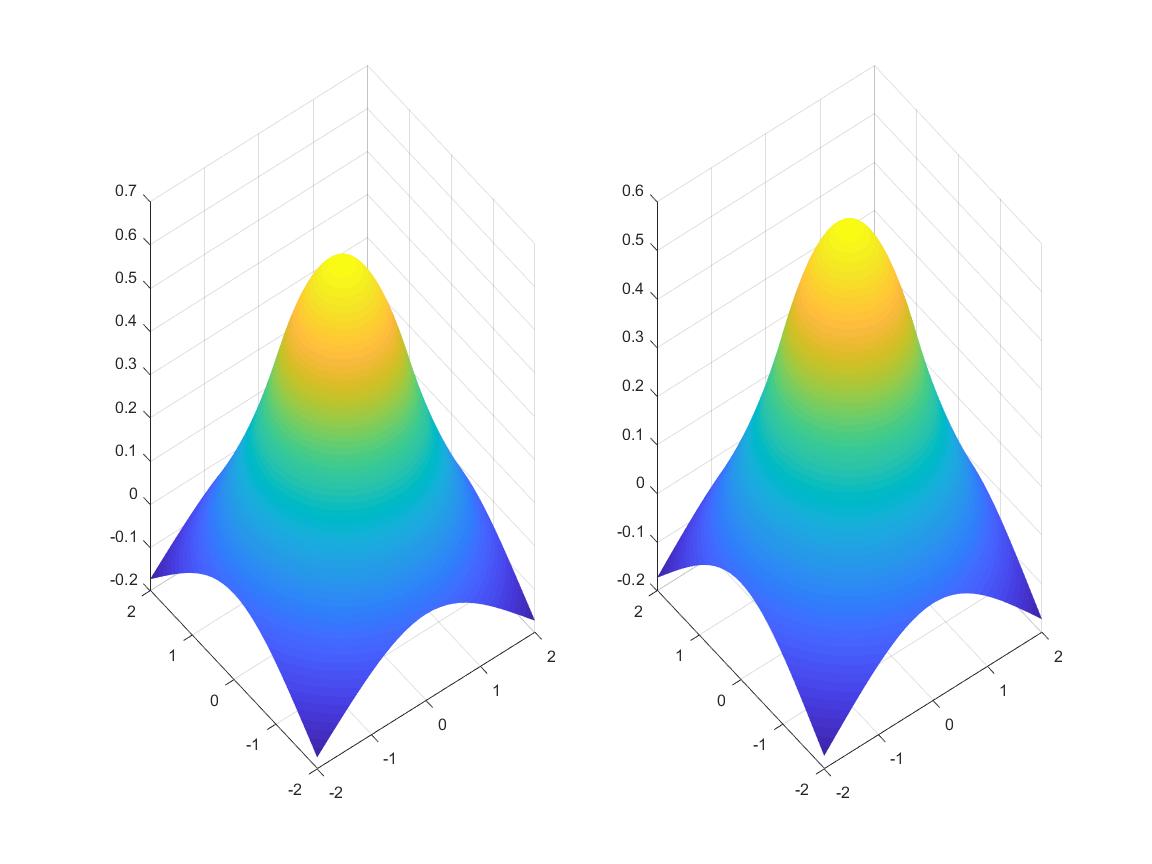
Figure 1: The profile of the discrete state(left) and the exact state(right) for Example 5.1 with $h=2^{-7}$.

References

• [1] V. Arnautu and P. Neittaanmäki, Discretization estimates for an elliptic control problem, Numer. Funct. Anal. Optim., 19(1998), pp. 431-464.
• [2] N. Arada, E. Casas and F. Tröltzsch, Error estimates for the numerical approximation of a semilinear elliptic control problem, Comput. Optim. Appl., 23(2002), pp. 201-229.
• [3] M. Bergounioux, K. Ito and K. Kunisch, Primal-dual strategy for constrained optimal control problems, SIAM J. Control Optim., 37(1999), pp. 1176-1194.
• [4] M. Bergounioux and K. Kunisch, Primal-dual strategy for state constrained optimal control problems, Comput. Optim. Appl., 22(2002), pp. 193-224.
• [5] M. Bergounioux and K. Kunisch, On the structure of Lagrange multipliers for state constrained optimal control problems, Systems Control Lett., 48(2003), pp. 169-176.
• [6] S. C. Brenner and L. Y. Sung, A new convergence analysis of finite element methods for elliptic distributed optimal control problems with pointwise state constraints, SIAM J. Control Optim., 55(2017), pp. 2289-2304.
• [7] S. C. Brenner, L. Y. Sung and Y. Zhang, A $C^{0}$ interior penalty method for an elliptic optimal control problem with state constraints, In Recent Developments in Discontinuous Galerkin Finite Element Methods for Partial Differential Equations (2012 John H. Barrett Memorial Lectures), X. Feng, O. Karakashian and Y. Xing, ed., IMA Volumes in Mathematics and Its Applications, 157(2013), pp. 97-132.
• [8] S. C. Brenner, L. Y. Sung, H. Zhang and Y. Zhang, A Morley finite element method for the displacement obstacle problem of clamped Kirchhoff plates, J. Comput. Appl. Math., 254(2013), pp. 31-42.
• [9] S. C. Brenner, T. Gudi, K. Porwal and L. Y. Sung, A Morley finite element method for an elliptic distributed optimal control problem with pointwise state and control constraints, ESIAM Control Optim. Calc. Var., 24(2018), pp. 1181-1206.
• [10] E. Casas, Control of an elliptic problem with pointwise state constraints, SIAM J. Control Optim., 24(1986), pp. 1309-1318.
• [11] E. Casas, Error estimates for the numerical approximation of semilinear elliptic control problems with finitely many state constraints, ESIAM Control Optim. Calc. Var., 8(2002), pp. 345-374.
• [12] E. Casas and M. Mateos, Uniform convergence of the FEM. Applications to state constrained control problems, Comput. Appl. Math., 21(2002), pp. 67-100.
• [13] E. Casas, M. Mateos and B. Vexler, New regularity results and improved error estimates for optimal control problems with state constraints, ESIAM Control Optim. Calc. Var., 20(2014), pp. 803-822.
• [14] E. Casas and L. A. Fernández, Optimal control of semilinear elliptic equations with pointwise constraints on the gradient of the state, Appl. Math. Optim., 27(1993), pp. 35-56.
• [15] E. Casas, C. Clason and K. Kunisch, Approximation of elliptic control problems in measure spaces with sparse solutions, SIAM J. Control Optim., 50(2012), pp. 1735-1752.
• [16] E. Casas, M. Mateos and F. Tr”oltzsch, Error estimates for the numerical approximation of boundary semilinear elliptic control problems, Comput. Optim. Appl., 31(2005), pp. 193-219.
• [17] E. Casas and M. Mateos, Error estimates for the numerical approximation of Neumann control problems, Comp. Appl. Math., 39(2008), pp. 265-295.
• [18] E. Casas and J. P. Raymond, Error estimates for the numerical approximation of Dirichlet boundary control for semilinear elliptic equations, SIAM J. Control Optim., 45(2006), pp. 1586-1611.
• [19] E. Casas and F. Tröltzsch, Error estimates for the finite element approximation of a semilinear elliptic control problems, Contr. Cybern. 31(2005), pp. 695-712.
• [20] E. Casas and M. Mateos, Uniform convergence of the FEM. Applications to state constrained control problems, Comp. Appl. Math., 21(2002), pp. 67-100.
• [21] E. Casas, M. Mateos and J. P. Raymond, Pontryagin’s principle for the control of parabolic equations with gradient state constraints, Nonlinear Anal., 46(2001), pp. 933-956.
• [22] C. Clason and K. Kunisch, A duality-based approach to elliptic control problems in non reflexive Banach spaces, ESAIM Control Optim. Calc. Var., 17(2011), pp. 243-266.
• [23] P. G. Ciarlet, The Finite Element Method for Elliptic Problems, North-Holland, Amsterdam, 1978.
• [24] K. Deckelnick, A. Günther and M. Hinze, Finite element approximation of Dirichlet boundary control for elliptic PDEs to two- and three-dimensional curved domains, SIAM J. Control Optim., 48(2009), pp. 2798-2819.
• [25] K. Deckelnick and M. Hinze. Convergence of a finite element approximation to a state-constrained elliptic control problem, SIAM J. Numer. Anal., 45(2007), pp. 1937-1953.
• [26] K. Deckelnick and M. Hinze. Numerical analysis of a control and state constrained elliptic control problem with piecewise constant control approximations, Proceeding of ENUMATH , 2007, pp. 597-604.
• [27] K. Deckelnick, A. Günther and M. Hinze, Finite element approximation of elliptic control problems with constraints on the gradient, Numer. Math., 111(2009), pp. 335-350.
• [28] R. Falk, Approximation of a class of optimal control problems with order of convergence estimates, J. Math. Anal. Appl., 44(1973), pp. 28-47.
• [29] R. Glowinski, Numerical Methods for Nonlinear Variational Problems, Springer-Verlag, New York, 1984.
• [30] R. Griesse and K. Kunisch, A semi-smooth newton method for solving elliptic equations with state constraints, ESAIM Math. Model. Numer. Anal.43(2009), pp. 209-238.
• [31] A. Günther and M. Hinze, Elliptic control problems with gradient constraints-variational discrete versus piecewise constant controls, Comput. Optim. Appl., 49(2011), pp. 549-566.
• [32] T. Geveci, On the approximation of the solution of an optimal control problem governed by an elliptic equation, RIARO Anal. Numér., 13 (1979), pp. 313-328.
• [33] R. Herzog and S. Mach, Preconditioned solution of state gradient constrained elliptic optimal control problems, SIAM J. Numer. Anal., 54(2016), pp. 688-718.
• [34] M. Hintermüller, M. Hinze and R. Hoppe, Weak-duality based adaptive finite element methods for PDE-constrained optimization with pointwise gradient state constraints, J. Comp. Math., 30(2012), pp. 101-123.
• [35] M. Hintermüller and K. Kunisch, PDE-Constrained optimization subject to pointwise constraints on the control, the state, and its derivative, SIAM J. Optim., 20(2009), pp. 1133-1156.
• [36] K. Ito and K. Kunisch, Lagrange Multiplier Approach to Variational Problems and Applications, Socity for Industrial and Applied Mathematics, Philadelphia, 2000.
• [37] D. Kinderlehrer and G. Stampacchia, An Introduction to Variational Inequalities and Their Applications, Society for industrial and Applied Mathematics, Philadelphia, 2000.
• [38] S. May and R. Rannacher and B. Vexler, A priori error analysis for the finite element approximation of elliptic Dirichlet boundary control problems, Proceeding of ENUMATH 2007, Graz (2008).
• [39] S. May and R. Rannacher and B. Vexler, Error analysis of a finite element approximation of elliptic Dirichlet boundary control problems, SIAM J. Control Optim., 51(2013), pp. 2585-2611.
• [40] C. Meyer and A. Rösch, $L^{\infty}$ estimates for approximated optimal control problems, SIAM J. Control Optim., 44(2005), pp. 1636-1649.
• [41] J. L. Lions, Optimal Control of Systems Governed by Partial Differential Equations, Springer-Verlag, Berlin, 1971.
• [42] W. B. Liu, N. N. Yan and W. Gong, A new finite element approximation of a state constrained optimal control problem, J. Comput. Math., 27(2009), pp. 97-114.
• [43] W. B. Liu, D. P. Yang, L. Yuan and C. Q. Gao, Finite element approximations of an optimal control problem with integral state constraint, SIAM J. Numer. Anal., 48(2010), pp. 1163-1185.
• [44] C. Meyer, Error estimates for the finite-element approximation of an elliptic control problem with pointwise state and control constraints, Control Cybern., 37(2008), pp. 51-83.
• [45] L. S. D. Morley, The triangular equilibrium problem in the solution of plate bending problems, Aero. Quart., 19(1968), pp. 149-169.
• [46] T. K. Nilssen, X. C. Tai and R. Winther, A robust nonconforming $H^{2}$-element, Math. Comp., 70(2000), pp. 489-505.
• [47] C. Ortner and W. Wollner, A priori error estimates for optimal control problems with pointwise constraints on the gradient of the state, Numer. Math., 118(2011), pp. 587-600.
• [48] A. Schiela and W. Wollner, Barrier methods for optimal control problems with convex nonlinear gradient state constraints, SIAM J. Optim., 21(2011), pp. 269-286.
• [49] P. Shakya and R. K. Sinha, A priori and a posteriori error estimates of finite element approximations for elliptic optimal control problem with measure data, Optim. Control Appl. Meth., 40(2019), pp. 241-264.
• [50] F. Tröltzsch, Optimal Control of Partial Differential Equations, AMS, Providence, RI, 2010.
• [51] W. Wollner, A posteriori error estimates for a finite element discretization of interior point methods for an elliptic optimization problem with state constraints, Comput. Optim. Appl., 47(2010), pp. 133-159.
• [52] W. Wollner, Optimal control of elliptic equations with pointwise constraints on the gradient of the state in nonsmooth polygonal domains, SIAM J. Control Optim., 50(2012), pp. 2117-2129.
• [53] J. Zhou and D. Yang, Legendre-Galerkin spectral methods for optimal control problems with integral constraint for state in one dimension, Comput. Optim. Appl., 61(2015), pp. 135-158.
• [54] L. Zhou, A priori error estimates for optimal control problems with state and control constraints, Optim. Control Appl. Meth., 39(2018), pp. 1168-1181.