Layer-Parallel Training of Residual Networks with Auxiliary-Variable Networks

Abstract

Gradient-based methods for the distributed training of residual networks (ResNets) typically require a forward pass of the input data, followed by back-propagating the error gradient to update model parameters, which becomes time-consuming as the network goes deeper. To break the algorithmic locking and exploit synchronous module parallelism in both the forward and backward modes, auxiliary-variable methods have attracted much interest lately but suffer from significant communication overhead and lack of data augmentation. In this work, a novel joint learning framework for training realistic ResNets across multiple compute devices is established by trading off the storage and recomputation of external auxiliary variables. More specifically, the input data of each independent processor is generated from its low-capacity auxiliary network (AuxNet), which permits the use of data augmentation and realizes forward unlocking. The backward passes are then executed in parallel, each with a local loss function that originates from the penalty or augmented Lagrangian (AL) methods. Finally, the proposed AuxNet is employed to reproduce the updated auxiliary variables through an end-to-end training process. We demonstrate the effectiveness of our methods on ResNets and WideResNets across CIFAR-10, CIFAR-100, and ImageNet datasets, achieving speedup over the traditional layer-serial training method while maintaining comparable testing accuracy.

Keywords: residual network, synchronous module-parallel training, penalty and augmented Lagrangian methods, optimal control of differential equations, auxiliary-variable network

1 Introduction

With the fast development of computer science and technology, learning with deep neural networks has enjoyed remarkable success across a wide variety of machine learning and scientific computing applications (LeCun et al., 2015; Brunton et al., 2020), where the backpropagation (BP) algorithm (Rumelhart et al., 1985) is widely adopted to fulfill the learning tasks. However, even with modern Graphical Processing Units (GPUs), the overall training process remains time-consuming, especially when the network is large and distributed across multiple computing devices.

To improve the training efficiency, various parallelization techniques such as the data-parallelism (Iandola et al., 2016), model-parallelism (Dean et al., 2012), and a combination of both (Paine et al., 2013; Harlap et al., 2018) have been proposed to reduce the training runtime. Unfortunately, none of these methods could fully overcome the scalability barrier created by the intrinsically serial propagation of data within the network itself (G$\ddot{\textnormal{u}}$nther et al., 2020), thereby forcing the distributed machines to work synchronously, and hence preventing us from fully leveraging the computing resources. In other words, the forward, backward, and update locking issues (Jaderberg et al., 2017) inherited from BP are not addressed by either of the methods above.

One way of breaking the algorithmic locks and achieving speed-up over the traditional layer-serial training strategies is to apply synthetic gradients to build decoupled neural interfaces (Jaderberg et al., 2017), where the true objective gradients are approximated by auxiliary neural networks so that each layer can be locally updated without performing the full serial BP. However, it fails in training deep convolutional neural networks since the construction of synthetic loss functions has little relation to the target loss function (Miyato et al., 2017). Nevertheless, this pioneering work motivates the continuing research on what later on became known as local error learning (see also the early work by (Mostafa et al., 2018) from a biological point of view). Recently, (Belilovsky et al., 2019, 2020; Löwe et al., 2019; Pyeon et al., 2020; Belilovsky et al., 2021) empirically demonstrate that we can apply this kind of method with carefully designed auxiliary neural networks to state-of-the-art networks training on real-world datasets, achieving comparable or even better performance against the benchmark BP approach. However, the loss function of these methods is no longer consistent with the original one, and the local worker can be short-sighted (Wang et al., 2021).

Another kind of method relies on the employment of delayed gradients for updating network parameters and therefore achieves backward unlocking (Huo et al., 2018b). However, this design suffers from large memory consumption and weight staleness introduced by the asynchronous backward updates, especially when the network goes deeper (Lian et al., 2015; Xu et al., 2020). To compensate for the gradient delay, feature replay (Huo et al., 2018a) stores all workers’ history inputs and then recomputes the latent feature map before executing the backward operations, which would incur extra computation time hampers the performance for the exposed parallelism. Besides, both methods fail to addresses the forward locking. Hence the acceleration is limited due to Amdahl’s law (Gustafson, 1988). As a potential solution, (Xu et al., 2020) suggests overlapping the recomputation with the forward pass to accelerate the training process further, leading to an asynchronous module parallelization. However, the forward dependency of a particular input data still exists.

To exploit synchronous module parallelism in both the forward and backward modes, several algorithms were proposed recently by introducing external auxiliary variables, e.g., the quadratic penalty method (Carreira-Perpinan and Wang, 2014; Zeng et al., 2018; Choromanska et al., 2018), the AL method (Taylor et al., 2016; Zeng et al., 2019; Marra et al., 2020) and the proximal method (Li et al., 2020) for training fully-connected networks, which can achieve speed-up over the traditional BP algorithm on a single Central Processing Unit (CPU) (Li et al., 2020). However, as shown in (Gotmare et al., 2018), the performances of most of these methods are much worse than that of BP for deep convolutional neural networks. In another recent approach (G$\ddot{\textnormal{u}}$nther et al., 2020; Parpas and Muir, 2019; Kirby et al., 2020), based on the similarity of ResNets training to the optimal control of nonlinear systems (E, 2017), parareal method for solving differential equations is employed to replace the forward and backward passes with iterative multigrid schemes. However, due to its necessity of recording both the state and adjoint variables to perform control updates, the implementation is difficult to integrate with the existing automatic differentiation technologies. Therefore, experiments were conducted on simple ResNets across small datasets rather than state-of-the-art ResNets across modern datasets. So far, to the best of our knowledge, it is still uncertain that whether we can effectively and efficiently apply these layer-parallel training strategies to modern deep ResNets training on real-world datasets.

Figure 1: A diagram describing the motivation of layer-parallel training algorithms from a dynamical systems view.

In this work, a novel layer-parallel training strategy is proposed by using low-capacity auxiliary-variable networks, which can achieve forward, backward, and update unlocking without explicitly storing the external auxiliary variables. As can be seen from Figure 1, our method is first motivated by the similarity of training ResNets to the optimal control of neural ODEs, which allows us to understand and break the algorithmic locking in the continuous-time sense. The corresponding discrete dynamical systems then offer us a fully decoupled training scheme, whereas the introduction of auxiliary networks permits the use of data augmentation by trading off storage and recomputation of the external auxiliary variables during training. More specifically, the proposed algorithm is constructed as follows (see also Figure 1):

• discrete to continuum: the deep layer limit of ResNet training task coincides with a terminal control problem governed by the so-called neural ordinary differential equations (ODE) (E, 2017; Haber and Ruthotto, 2017; Thorpe and van Gennip, 2018);

• penalty or augmented Lagrangian method: the penalty or AL method (Maday and Turinici, 2002; Nocedal and Wright, 2006) is employed for the approximate solution of the neural ODE-constrained optimal control problem, which breaks the forward, backward, and update locking in the continuous-time sense;

• continuum to discrete: a consistent finite difference scheme (Gholami et al., 2019) is adopted for the discrete-in-time solution of the relaxed problem in the previous step, leading to a layer-parallel training algorithm with external auxiliary variables;

• trade-off between storage and computation: to enable the use of data augmentation for improving model performance, the low-capacity AuxNet is trained to learn the correlation between auxiliary variables by replicating their values at each iteration.

The rest of this paper is organized as below. Section 2 is devoted to reviewing the classical BP algorithm and its locking issues, followed by the layer-serial training of deep ResNets from a dynamical systems viewpoint. Then a brief survey of related work on removing these limitations is presented. Next, in section 3, the penalty and AL methods are illustrated to achieve forward, backward, and update unlocking in the continuous-time sense. Its discrete-time counterpart is presented in section 4. Experimental results are reported in section 5 to demonstrate the effectiveness and efficiency of our methods, followed by some concluding remarks and future improvements in section 6.

2 Background and Related Work

In this section, we begin by briefly reviewing the most commonly used BP algorithm (Hecht-Nielsen, 1992) for training deep ResNets (He et al., 2016a, b), followed by a concise description of its locking effects (Jaderberg et al., 2017) from the dynamical system view (Li et al., 2017). Then a survey of related work on breaking these algorithmic limitations (i.e., the forward, backward, and update lockings) is presented and compared with our current work.

2.1 Layer-Serial Training From a Dynamical Systems View

Figure 2: A diagram describing the layer-serial training process of a pre-activation ResNet.

We consider the benchmark residual learning framework (He et al., 2016a, b) that assigns pixels in the raw input image to categories of interest as depicted in Figure 2. Specifically, given a human-labeled database $\{y,h(y)\}_{y\in\Omega}$, the learning task requires solving the optimization problem

$$\operatorname*{arg\,min}_{\{W_{\ell}\}_{\ell=0}^{L-1}}\left\{\varphi(X_{L})\,\Big{|}\,X_{0}=S(y),\ X_{\ell+1}=X_{\ell}+F(X_{\ell},W_{\ell})\ \,\textnormal{for}\ 0\leq\ell\leq L-1\right\}$$ (1)

where $\displaystyle\varphi(X_{L})=\mathbb{E}_{y\in\Omega}\!\Big{[}\lVert T(X_{L})-h(y)\rVert\Big{]}$ represents the classification loss function, $X_{\ell}$ the input feature map of the $\ell$-th residual block, $L\in\mathbb{N}_{+}$ the total number of building blocks, $F$ typically a composition of linear and nonlinear functions as depicted in Figure 2, $W_{\ell}$ the network parameters to be learned, and $\lVert\cdot\rVert$ a given metric measuring the discrepancy between the model prediction $T(X_{L})$ and the ground-truth label $h(y)$ for each input image $y\in\Omega$. The trainable parameters of input and output layers, i.e., $S$ and $T$ in Figure 2, are assumed to be fixed (Haber et al., 2018) for the ease of illustration.

Based on the concept of modified equations (E, 2017) or the variational analysis using $\Gamma$-convergence (Thorpe and van Gennip, 2018), the learning task (1) can be interpreted as the discretization of a terminal control problem governed by the so-called neural ordinary differential equation (Chen et al., 2018)

$$\operatorname*{arg\,min}_{\omega_{t}}\left\{\varphi(x_{1})\,\Big{|}\,x_{0}=S(y),\,dx_{t}=f(x_{t},w_{t})dt\ \,\textnormal{for}\ 0<t\leq 1\right\}.$$ (2)

Accordingly, the continuous-in-time counterpart of the most commonly used BP algorithm (Hecht-Nielsen, 1992) for solving (1), namely,

$$W_{\ell}\leftarrow W_{\ell}-\eta\frac{\partial\varphi(X_{L})}{\partial X_{\ell+1}}\frac{\partial X_{\ell+1}}{\partial W_{\ell}},\qquad 0\leq\ell\leq L-1,$$ (3)

is handled by the adjoint and control equations for finding the extremal of (2) (Li et al., 2017), that is, for $0\leq t\leq 1$,

$$dp_{t}=-p_{t}\frac{\partial f(x_{t},w_{t})}{\partial x}dt,\qquad p_{1}=\frac{\partial\varphi(x_{1})}{\partial x},$$ (4)

$$w_{t}\leftarrow w_{t}-\eta p_{t}\frac{\partial f(x_{t},w_{t})}{\partial w},$$ (5)

where $\eta>0$ represents the learning rate and $p_{t}$ the adjoint (or co-state) variable that captures the loss changes with respect to hidden activation layers (see Appendix A and Appendix B for more details).

Notably, as the training datasets and modern neural networks are becoming larger and larger, a single machine can no longer meet the memory and computing demands placed on it, leading to a need for distributed training. As an illustrative example, the top figure in Table 1 shows a partitioning of the deep ResNet (1) across three machines, where the conventional BP algorithm (3) with stochastic gradient descent optimization technique (Bottou, 2010) is adopted for training. Clearly, such a straightforward implementation would result in several forms of locking (Jaderberg et al., 2017), that is,

• forward locking: for each input mini-batch, no worker can process its corresponding incoming data before the previous node in directed forward network have executed;

• backward locking: no worker can capture the loss changes with respect to its hidden activation layers before the previous node in the backward network have executed;

• update locking: no worker can update its trainable parameters before all the dependent nodes have executed in both the forward and backward modes;

which results in severe under-utilization of computing resources. More specifically, as can be seen from the top figure in Table 1, only a single machine is active at any instant of time, leading to a V-shaped cycle with lots of idle machines over the entire training process.

It is noteworthy that these locking issues for training deep ResNets can be recast as the necessity of first solving the forward-in-time neural ODE in (2) and then the backward-in-time adjoint (or co-state) equation (4) in order to perform the control updates (5) (E, 2017; Li et al., 2017). This connection not only brings us a dynamical system view of the locking effects but also provides a way to consistently discretize the iterative system (4-5) for solving the time-serial training problem (2).

Method	Training Progress (across 3 workers with 3 mini-batches displayed)
BP
PipeDream
Gpipe
DDG
FR
Sync-DGL
Async-DGL
Our Method
Notation Description

Table 1: Timelines of different strategies to accelerate the neural network training process (runtime and per-worker utilization are shown along the $x$- and $y$-axes). For each worker, the backward pass is assumed to take twice as long as the forward one.

2.2 Related Works

For models that are too large to store in a single worker’s memory or cache, some representative works on breaking the forward, backward, and update locking issues are briefly reviewed and summarized in this section, as illustrated in Table 1 and Table 2.

Backpropagation: Due to the necessity of first executing the forward pass of (1) and then the backward gradient propagation (31) in order to perform parameter updates (30) (also known as the forward, backward, and update locking, respectively) at each iteration step, the conventional BP algorithm (Hecht-Nielsen, 1992) for training deep neural networks forces the distributed machines to work in a synchronous fashion (see the top figure in Table 1), thereby compromising the efficiency of computing resources.

Pipeline Parallelism: To accelerate the distributed training process, PipeDream (Harlap et al., 2018; Narayanan et al., 2019, 2021) and GPipe (Huang et al., 2019) propose the pipelined model parallelism so that multiple input data can be pushed through all the available workers in a sequential order. To be specific, PipeDream pipelines the execution of forward passes and intersperses them with BPs in an attempt to minimize the processor idle time. However, such an asynchronous approach introduces inconsistent parameter updates between the forward and backward passes of a particular input (see Table 1 and (30)), requiring more effort to compute the gradient accurately (Narayanan et al., 2021). On the other hand, GPipe divides the input mini-batch into smaller micro-batches (not relabeled in Table 1) and updates parameter after accumulating all the micro-batch gradients, which can be regarded as a combination of model parallelism and data parallelism.

Unfortunately, the locking issues inherited from the forward-backward propagation of data across all the network layers are not addressed by the pipeline parallelism. Therefore, exploring dimensions beyond the data and model parallelism may potentially further accelerate the network training.

Delayed Gradients: Note that the backward pass takes roughly twice as long as the forward one, which motivates the pursuit of removing the backward locking. (Huo et al., 2018b) proposes decoupled parallel backpropagation (DDG), achieving backward unlocking by applying delayed gradients for parameter updates. However, this design is known to suffer from large memory consumption and weight staleness (see Table 1) introduced by asynchronous backward updates, especially when the network goes further deeper (Lian et al., 2015; Xu et al., 2020). To compensate the gradient delay (see Table 1), feature replay (FR) (Huo et al., 2018a) stores the history inputs of all workers and recompute the hidden activations before executing the backward operations, which would incur additional computation time. Besides, neither DDG nor FR addresses the issue of forward locking, hence the acceleration is limited due to the Amdahl’s law (Gustafson, 1988). (Xu et al., 2020) suggests to overlap the recomputation with the forward pass to further reduce the runtime, however, the forward dependency of a particular input data still exists.

Local Error Learning: Another effective way of removing the backward locking is to artificially build local loss functions so that the trainable parameters of each individual worker can be locally updated without performing the full layer-serial BP. One of the pioneer works is the decoupled neural interface (Jaderberg et al., 2017), which employs auxiliary neural networks to generate synthetic gradients for the decoupled backward pass. However, it fails in training deep convolutional neural networks since the auxiliary local loss function has little relation to the target objective function (Miyato et al., 2017). To further reduce the discrepancy between the synthetic and exact gradients, (Mostafa et al., 2018) suggests to use local classifiers with cross-entropy loss for the backward propagation, while a similarity measure combined with the local classifier is introduced in (Nøkland and Eidnes, 2019). Recently, (Belilovsky et al., 2019, 2020; Löwe et al., 2019; Pyeon et al., 2020) empirically demonstrate that this kind of method with carefully designed auxiliary networks can be applied to modern deep networks across real-world datasets, achieving comparable or even better performance against the standard BP. More specifically, as can be seen from Table 1, the synchronous decoupled greedy learning (Sync-DGL) (Belilovsky et al., 2020) attaches each worker with a small auxiliary network that generates its own gradients for BP, which allows achieving backward unlocking. Moreover, by making use of a replay buffer for each worker, forward unlocking can be achieved but in an asynchronous fashion (see the Async-DGL in Table 1).

However, the objective function of local error learning methods is no longer consistent with the original one (1), or in other words, the actual problem has been changed to another one by these methods. In this way, perhaps it is more appropriate to say that these methods themselves do not suffer from the forward, backward, and update locking, rather than breaking the locking issues of the baseline model (1). Another sacrifice that local error learning has to make is the introduction of auxiliary networks with extra trainable parameters, forcing the workers to be short-sighted and learn features that only benefit local layers (Wang et al., 2021).

Auxiliary Variable Methods: To exploit model parallelism in both the forward and backward modes, one can also consider the use of external auxiliary variables for distributed training, e.g., the quadratic penalty method (Choromanska et al., 2018; Zeng et al., 2018; Carreira-Perpinan and Wang, 2014), the augmented Lagrangian method (Taylor et al., 2016; Zeng et al., 2019; Marra et al., 2020), and the proximal method (Li et al., 2020) for training fully-connected networks, which can achieve speed-up over the traditional layer-serial training strategy on a single Central Processing Unit (CPU) (Li et al., 2020). However, as shown in (Gotmare et al., 2018), the performances of most of these methods are much worse than that of BP for deep convolutional neural networks. On the other hand, based on the similarity of ResNets training to the optimal control of nonlinear systems (E, 2017), the parareal method for solving differential equations is employed to replace the conventional forward-backward propagation with iterative multigrid schemes (G$\ddot{\textnormal{u}}$nther et al., 2020; Parpas and Muir, 2019; Kirby et al., 2020). Although the locking issues can be resolved, the implementation is complicated and difficult to integrate with the existing library technologies such as BP and automatic differentiation. Therefore, experiments were conducted on the simple ResNets across small datasets (Kirby et al., 2020), rather than the state-of-the-art ResNets across larger datasets.

So far, to the best of our knowledge, it is still uncertain that whether these auxiliary variable methods can be effectively and efficiently applied to modern deep networks across real-world datasets, which motivates us to combine the benefits of all these technologies and develop a novel layer-parallel training method using auxiliary variable networks. To be specific, as can be seen from Table 1, the input data of each worker is induced from its corresponding auxiliary variable networks, which permits the use of data augmentation at a low cost and achieves forward unlocking. Then the backward passes are executed synchronously in parallel, each with a local loss function that originates from the penalty or AL methods (see Figure 1).

Method	​​ Model Solution	Module Unlocking			Forward Independency	Auxiliary Request
		Forward	Backward	Update		Memory	Network
BP	$\surd$	$\times$	$\times$	$\times$	$\times$	$\times$	$\times$
PipeDream	$\surd$	$\times$	$\times$	$\times$	$\times$	$\times$	$\times$
Gpipe	$\surd$	$\times$	$\times$	$\times$	$\times$	$\surd$	$\times$
DDG	$\surd$	$\times$	$\surd$	$\surd$	$\times$	$\surd$	$\times$
FR	$\surd$	$\times$	$\surd$	$\surd$	$\times$	$\surd$	$\times$
​ Sync-DGL ​	$\times$	$\times$	$\surd$	$\surd$	$\times$	$\times$	$\surd$
​ Async-DGL ​	$\times$	$\surd$	$\surd$	$\surd$	$\times$	$\surd$	$\surd$
​ Our Method ​	$\surd$	$\surd$	$\surd$	$\surd$	$\surd$	$\times$	$\surd$

Table 2: Comparison of different model-parallel training methods in terms of model solution, module unlocking, forward independency and auxiliary request.

To sum up, Table 2 compares our method with other representative works in terms of several criteria, all of which can not only decouple the traditional layer-serial training process but also show potential to match the performance of a standard BP in real-world applications. In either case, the training strategy should be consistent with the default baseline model (1) for fair comparison, which we refer to as model solution in Table 2. It is noteworthy that although the forward unlocking can be achieved by allowing the workers to operate asynchronously on different mini-batches (e.g., the Async-DGL in Table 1), the forward pass of a particular mini-batch still remains sequential across multiple compute devices. For the ease of illustration, removing such a specific forward locking is called forward independency in Table 2. On the other hand, backward unlocking would permit the decoupled BP running in parallel once the local forward pass is completed, while update unlocking would allow updates of model parameters before all subsequent modules complete executing the forward propagation. Besides, the common sacrifice for achieving module-parallelism is the introduction of auxiliary memory footprints or neural networks, which is summarized in the last two columns of Table 2. Clearly, our method surpasses the other algorithms in terms of the first five criteria, but comes at the cost of incorporating auxiliary networks. Fortunately, the extra trainable parameters imposed by these auxiliary networks are of small size, which is empirically demonstrated in section 5.

3 Time-Parallel Training

Based on the analysis of forward, backward, and update locking effects in section 2, we are now ready to break these algorithmic limitations in the continuous-time sense, i.e., the second path in Figure 1. More specifically, to avoid the necessity of solving forward-backward differential equations for performing control updates at each iteration step (see (32) in Appendix B), constraint violations through the use of penalty and AL methods (Nocedal and Wright, 2006; Maday and Turinici, 2002; Carraro et al., 2015) are introduced in this section, which also paves the way for increasing the concurrency of the network training process.

Figure 3: Contrary to the trajectory of neural ODE (blue line), introducing external auxiliary variables at certain moments (solid red dots) enables a time-parallel computation of the state (red lines), adjoint, and control variables. However, to approximately recover the original dynamic, violation of equality constraints (mismatch between the solid and hollow red dots) should be penalized in the loss function.

3.1 Forward Pass with Auxiliary Variables

To employ $K\in\mathbb{N}_{+}$ independent processors for the forward-in-time evolution of the neural ODE in (2), we introduce a coarse partition of $[0,1]$ into several disjoint intervals as shown in Figure 3, that is,

$$0=s_{0}<\ldots<s_{k}<s_{k+1}<\ldots<s_{K}=1.$$

Now we are ready to define the piecewise state variables $\{x_{t}^{k}\}_{k=0}^{K-1}$ such that the underlying dynamic evolves according to

$$x^{k}_{s_{k}^{+}}=\lambda_{k},\qquad dx^{k}_{t}=f(x^{k}_{t},w^{k}_{t})dt\ \ \ \textnormal{on}\ (s_{k},s_{k+1}],$$ (6)

i.e., the continuous-time forward pass that originates from external auxiliary variable $\lambda_{k}$ and with control variable $w_{t}^{k}$. Here, and in what follows, $x^{k}_{s_{k}^{+}}$ and $x^{k}_{s_{k}^{-}}$ refer to the right and left limits of the possibly discontinuous function $x^{k}_{t}$ at the time interface $t=s_{k}$.

Clearly, for any $t\in[s_{k},s_{k+1}]$ where $0\leq k\leq K-1$, the state solution of time-serial training method (2) satisfies $x_{t}=x^{k}_{t}$ if and only if

$$w_{t}^{k}=w_{t}|_{(s_{k},s_{k+1})}\qquad\textnormal{and}\qquad\lambda_{k}=x_{s_{k}^{+}},$$

or by defining $x^{-1}_{s_{0}^{-}}=x_{0}$, we arrive at an equivalent form of the above conditions

$$w_{t}^{k}=w_{t}|_{(s_{k},s_{k+1})}\qquad\textnormal{and}\qquad\lambda_{k}=x^{k-1}_{s_{k}^{-}}.$$

As an immediate result, the optimization problem (2) can be reformulated as

$$\begin{gathered}\operatorname*{arg\,min}_{\{w^{k}_{t}\}_{k=0}^{K-1}}\left\{\varphi(x^{K-1}_{s_{K}^{-}})\,\Big{|}\,x^{k-1}_{s_{k}^{-}}=\lambda_{k}\ \ \text{and}\ \ x^{k}_{s_{k}^{+}}=\lambda_{k},\ \,dx^{k}_{t}=f(x^{k}_{t},w^{k}_{t})dt\ \ \textnormal{on}\ (s_{k},s_{k+1}]\right\}\end{gathered}$$ (7)

which offers the possibility of parallelizing the piecewise neural ODEs (6) by removing the other constraint. To be specific, the exact connection between adjacent sub-intervals can be loosened by incorporating external auxiliary variables (see Figure 3), which inspires us to relax the first constraint in (7) and add penalties to the objective loss function, i.e.,

$$\operatorname*{arg\,min}_{\{w_{t}^{k},\lambda_{k}\}_{k=0}^{K-1}}\bigg{\{}\varphi(x^{K-1}_{s_{K}^{-}})+\beta\sum_{k=0}^{K-1}\psi(\lambda_{k},x^{k-1}_{s_{k}^{-}})\,\Big{|}\,x^{k}_{s_{k}^{+}}=\lambda_{k},\ \,dx^{k}_{t}=f(x^{k}_{t},w^{k}_{t})dt\ \ \textnormal{on}\ (s_{k},s_{k+1}]\bigg{\}}$$ (8)

where $\beta>0$ is a scalar constant and $\psi(\lambda,x)=\|\lambda-x\|_{\ell_{2}}^{2}$ the penalty function.

3.2 Penalty Method

Note that, by definition, $\psi(\lambda_{0},x^{-1}_{s_{0}^{-}})=\psi(x_{0},x_{0})=0$. The Lagrange functional (Liberzon, 2011) associated with the optimization problem (8), i.e.,

$$\mathcal{L}_{\textnormal{P}}(x_{t}^{k},p_{t}^{k},w^{k}_{t},\lambda_{k})=\varphi(x^{K-1}_{s_{K}^{-}})+\sum_{k=0}^{K-1}\left(\beta\psi(\lambda_{k},x^{k-1}_{s_{k}^{-}})+\int_{s_{k}}^{s_{k+1}}p^{k}_{t}\big{(}f(x_{t}^{k},w^{k}_{t})-\dot{x}_{t}^{k}\big{)}dt\right)$$

implies that the adjoint variable $p_{t}^{k}$ satisfies a backward-in-time differential equation

$$\begin{array}[]{l}\displaystyle dp_{t}^{k}=-p_{t}^{k}\frac{\partial f(x_{t}^{k},w^{k}_{t})}{\partial x}dt\ \ \ \textnormal{on}\ [s_{k},s_{k+1}),\\ \displaystyle p^{k}_{s_{k+1}^{-}}=\left(1-\delta_{k,K-1}\right)\beta\frac{\partial\psi(\lambda_{k+1},x^{k}_{s_{k+1}^{-}})}{\partial x}+\delta_{k,K-1}\,\frac{\partial\varphi(x^{k}_{s_{k+1}^{-}})}{\partial x},\end{array}$$ (9)

for any $0\leq k\leq K-1$. Here, the notation $\delta_{k,K-1}$ (or $\delta$ for short) indicates the Kronecker Delta function throughout this work.

Similar to (5), the update rule for the piecewise control variables of (8) follows from

$$w_{t}^{k}\leftarrow w_{t}^{k}-\eta p_{t}^{k}\frac{\partial f(x_{t}^{k},w^{k}_{t})}{\partial w}\ \ \ \textnormal{on}\ [s_{k},s_{k+1}],$$ (10)

where $0\leq k\leq K-1$, and various gradient-based approaches (Gotschel and Minion, 2019; Nocedal and Wright, 2006) can be applied for the correction of auxiliary variables, e.g.,

$$\lambda_{0}\equiv x_{0}\ \ \ \textnormal{and}\ \ \ \lambda_{k}\leftarrow\lambda_{k}-\eta\left(\beta\frac{\partial\psi(\lambda_{k},x^{k-1}_{s_{k}^{-}})}{\partial\lambda}+p^{k}_{s_{k}^{+}}\right)\ \ \textnormal{for}\ 1\leq k\leq K-1.$$ (11)

To sum up, the penalty method for approximating the time-serial training procedure (2) at each iteration consists of

which breaks the forward, backward, and update locking in the continuous-time sense.

In particular, by choosing the quadratic penalty function $\psi(\lambda,x)=\lVert\lambda-x\rVert_{\ell_{2}}^{2}$, it can be deduced from (11) that the constraint violations of the approximate minimizer to (8) satisfy

$$\lambda_{0}-x^{-1}_{s_{0}^{-}}=0\ \ \ \textnormal{and}\ \ \ \lambda_{k}-x^{k-1}_{s_{k}^{-}}\approx-\frac{1}{2\beta}p^{k}_{s_{k}^{+}}\ \ \textnormal{for}\ 1\leq k\leq K-1,$$ (12)

which implies that a relatively large penalty coefficient $\beta$ is needed in order to force the minimizer of (8) close to the feasible region of our original problem (2). Such a quadratic penalty method has been extensively employed due to its simplicity and intuitive appeal (Gotmare et al., 2018; Choromanska et al., 2018), however, it suffers from well-known limitations such as numerical ill-conditioning due to the large penalty coefficients (Nocedal and Wright, 2006), memory issue of storing all the external auxiliary variables, and poor quality for feature extraction (Gotmare et al., 2018). Alternatively, the nonsmooth exact penalty method, e.g., $\psi(\lambda,x)=\lVert\lambda-x\rVert_{\ell_{1}}$ or $\lVert\lambda-x\rVert_{\ell_{\infty}}$, can often find a solution by performing a single unconstrained minimization, but the non-smoothness may create complications (Nocedal and Wright, 2006). In addition, the schedule of penalty coefficient is often different for different datasets, hence a wise strategy for choosing penalty function and coefficient is of crucial importance to the practical performance.

3.3 Augmented Lagrangian Method

To make the approximate solution of (8) nearly satisfy the dynamic (7) even for moderate values of penalty coefficient $\beta$, we consider the AL functional

$$\mathcal{L}_{\textnormal{AL}}(x_{t}^{k},p_{t}^{k},w^{k}_{t},\lambda_{k},\kappa_{k})=\mathcal{L}_{\textnormal{P}}(x_{t}^{k},p_{t}^{k},w^{k}_{t},\lambda_{k})-\sum_{k=0}^{K-1}\kappa_{k}(\lambda_{k}-x^{k-1}_{s_{k}^{-}})$$ (13)

where $\kappa_{k}$ denotes an explicit Lagrange multiplier associated with the $k$-th continuity-constraint of (7). Notably, by forcing $\kappa_{k}\equiv 0$ for all $0\leq k\leq K-1$, the AL method degenerates the penalty approach established in the previous section.

Then, by calculus of variations (Liberzon, 2011), the adjoint variable $p_{t}^{k}$ is shown to satisfy the backward-in-time differential equations (see Appendix C for more details)

$$\begin{array}[]{l}\displaystyle dp_{t}^{k}=-p_{t}^{k}\frac{\partial f(x_{t}^{k},w^{k}_{t})}{\partial x}dt\ \ \ \textnormal{on}\ [s_{k},s_{k+1}),\\ \displaystyle p^{k}_{s_{k+1}^{-}}=\left(1-\delta_{k,K-1}\right)\Bigg{(}\beta\frac{\partial\psi(\lambda_{k+1},x^{k}_{s_{k+1}^{-}})}{\partial x}+\kappa_{k+1}\Bigg{)}+\delta_{k,K-1}\,\frac{\partial\varphi(x^{k}_{s_{k+1}^{-}})}{\partial x},\end{array}$$ (14)

for any $0\leq k\leq K-1$, while the update rule for control variables is given by

$$w_{t}^{k}\leftarrow w_{t}^{k}-\eta p_{t}^{k}\frac{\partial f(x_{t}^{k},w^{k}_{t})}{\partial w}\ \ \ \textnormal{on}\ [s_{k},s_{k+1}]$$ (15)

for $0\leq k\leq K-1$, and the correction of auxiliary variables now takes on the form

$$\lambda_{0}\equiv x_{0}\ \ \ \textnormal{and}\ \ \ \lambda_{k}\leftarrow\lambda_{k}-\eta\left(\beta\frac{\partial\psi(\lambda_{k},x^{k-1}_{s_{k}^{-}})}{\partial\lambda}+p^{k}_{s_{k}^{+}}-\kappa_{k}\right)\ \ \textnormal{for}\ 1\leq k\leq K-1.$$ (16)

Similar to the analysis for penalty method, by choosing $\psi(\lambda,x)=\lVert\lambda-x\rVert_{\ell_{2}}^{2}$, formula (16) implies that the constraint violations of augmented Lagrangian method satisfy

$$\lambda_{0}-x^{-1}_{s_{0}^{-}}=0\ \ \ \textnormal{and}\ \ \ \lambda_{k}-x^{k-1}_{s_{k}^{-}}\approx\frac{1}{2\beta}(\kappa_{k}-p^{k}_{s_{k}^{+}})\ \ \textnormal{for}\ 1\leq k\leq K-1$$ (17)

which offers two ways of improving the consistency constraint $x^{k-1}_{s_{k}^{-}}=x^{k}_{s_{k}^{+}}$: increasing $\beta$ or sending $\kappa_{k}\to p^{k}_{s_{k}^{+}}$, whereas the penalty method (12) provides only one option. As an immediate consequence, the ill-conditioning of quadratic penalty method can be avoided without increasing $\beta$ indefinitely. Under such circumstances, the update rule for explicit Lagrange multipliers can be deduced from (17), namely,

$$\kappa_{0}\equiv 0\ \ \ \textnormal{and}\ \ \ \kappa_{k}\leftarrow\kappa_{k}-\frac{\eta}{2\beta}\big{(}\lambda_{k}-x^{k-1}_{s_{k}^{-}}\big{)}\ \ \textnormal{for}\ 1\leq k\leq K-1.$$ (18)

To sum up, the essential ingredients of AL method for approximately solving the time-serial training problem (2) at each iteration includes

which also parallelizes the time-serial iterative system (32) and hence realizes the forward, backward, and update unlocking in the continuous-time sense. Moreover, by employing the AL method, the ill-conditioning of quadratic penalty method (12) can be lessened without increasing the penalty coefficient indefinitely. However, the introduction of explicit Lagrangian multipliers may require additional memory and communication overheads that need to be properly handled (see more discussion in the following section).

4 Layer-Parallel Training

According to the stable finite difference schemes discussed in Section 2.1 (or see reference (Gholami et al., 2019)), we are now ready to discretize the time-parallel training problem (8) into local optimization processes and establish a non-intrusive layer-parallel training algorithm, i.e., the third path in Figure 1. Note that the external auxiliary variables can increase concurrency across all the building modules but would incur additional memory and communication overheads, which makes it quite challenging to cooperate with the indispensable data augmentation techniques (Tanner and Wong, 1987). Therefore, auxiliary-variable networks are proposed and deployed recursively to balance the storage overhead and the computation time, which enables the use of data augmentation for improving the performance of trained models.

4.1 Decoupled Forward Pass and Backpropagation

Recall the partitioning of $[0,1]$ associated with the layer-serial training task (1), i.e.,

$$0=t_{0}<t_{1}<\ldots<t_{\ell}=\ell\Delta t<t_{\ell+1}<\ldots<t_{L}=1,$$

its decomposed counterpart (see also Section 3.1) is built by choosing a coarsening factor $n\in\mathbb{N}_{+}$ and extracting every $n$-th building block as depicted in Figure 3

$$0=s_{0}<\ldots<s_{k}=t_{nk}<s_{k+1}<\ldots<s_{K}=1,$$

namely, the network architecture within each coarse interval $[s_{k},s_{k+1}]$ is constructed with a stack of $n$ residual blocks.

To be specific, $[s_{k},s_{k+1}]$ can be uniformly divided into $n$ sub-intervals

$$s_{k}=t_{kn}<t_{kn+1}<\cdots<t_{kn+n-1}<t_{kn+n}=s_{k+1},$$

for $0\leq k\leq K-1$, and we have by (6) that the feature flow now evolves according to

$$X_{kn}^{k}=\lambda_{k},\ \ \ X_{kn+m+1}^{k}=X_{kn+m}^{k}+F(X_{kn+m}^{k},W^{k}_{kn+m})$$ (19)

where $0\leq m\leq n-1$, which can be executed in parallel across $K$ computing processors.

Next, by employing the particular numerical schemes (31) that arise from the discrete-to-continuum analysis (see Appendix B) and equation (19), the discretization of our adjoint equation (14) is given by the backward dynamic

$$\begin{array}[]{l}\displaystyle P_{kn+m}^{k}=P_{kn+m+1}^{k}+P_{kn+m+1}^{k}\frac{\partial F(X_{kn+m}^{k},W^{k}_{kn+m})}{\partial X}=P_{kn+m+1}^{k}\frac{\partial X^{k}_{kn+m+1}}{\partial X^{k}_{kn+m}},\\ \displaystyle P_{kn+n}^{k}=(1-\delta_{k,K-1})\left(\beta\frac{\partial\psi(\lambda_{k+1},X^{k}_{kn+n})}{\partial X^{k}_{kn+n}}+\kappa_{k+1}\right)+\delta_{k,K-1}\frac{\partial\varphi(X_{kn+n}^{k})}{\partial X^{k}_{kn+n}}.\end{array}$$ (20)

Or, equivalently, for any $0\leq k\leq K-1$ and $0\leq m\leq n$, the discrete adjoint variable in (20) can be reformulated as

$$P_{kn+m}^{k}=(1-\delta_{k,K-1})\left(\beta\frac{\partial\psi(\lambda_{k+1},X^{k}_{kn+n})}{\partial X^{k}_{kn+m}}+\kappa_{k+1}\frac{\partial X^{k}_{kn+n}}{\partial X^{k}_{kn+m}}\right)+\delta_{k,K-1}\frac{\partial\varphi(X_{kn+n}^{k})}{\partial X^{k}_{kn+m}}$$ (21)

which captures the terminal and intermediate loss changes, i.e., the second- and first-term on the right-hand-side of (21), with respect to the hidden activation layers for $k=K-1$ and $0\leq k\leq K-2$, respectively.

In contrast to the traditional method (Maday and Turinici, 2002; G$\ddot{\textnormal{u}}$nther et al., 2020) where the control updates are performed after finding all the discrete state and adjoint variables, we propose to conduct control updates (15) right after the numerical solution of the adjoint equation (14) at each time slice. More specifically, by recalling (5) and (30), we have, for any $0\leq k\leq K-1$ and $0\leq m\leq n$, that the parameter updates associated with the $k$-th stacked modules can be deduced from (15), (19), and (21), i.e.,

$$\begin{split}W_{kn+m}^{k}\leftarrow\ &W_{kn+m}^{k}-\eta P^{k}_{kn+m+1}\frac{\partial F(X^{k}_{kn+m},W^{k}_{kn+m})}{\partial W}\\ =\ &W^{k}_{kn+m}-\eta\bigg{(}(1-\delta_{k,K-1})\bigg{(}\beta\frac{\partial\psi(\lambda_{k+1},X^{k}_{kn+n})}{\partial W^{k}_{kn+m}}+\kappa_{k+1}\frac{\partial X^{k}_{kn+n}}{\partial W^{k}_{kn+m}}\bigg{)}\\ &\qquad\qquad\ \ \ \ \ +\delta_{k,K-1}\frac{\partial\varphi(X_{kn+n}^{k})}{\partial W^{k}_{kn+m}}\bigg{)}\end{split}$$ (22)

which can not only be executed in parallel but also guarantee the accuracy of gradient information (Gholami et al., 2019).

On the other hand, we have by (16) and (21) that the correction of auxiliary variables satisfies $\lambda_{0}\equiv x_{0}$ and

$$\begin{split}\lambda_{k}\leftarrow\lambda_{k}-\eta&\bigg{(}\beta\frac{\partial\psi(\lambda_{k},X^{k-1}_{kn})}{\partial\lambda}+(1-\delta_{k,K-1})\bigg{(}\beta\frac{\partial\psi(\lambda_{k+1},X^{k}_{kn+n})}{\partial X^{k}_{kn}}+\kappa_{k+1}\frac{\partial X^{k}_{kn+n}}{\partial X^{k}_{kn}}\bigg{)}\\ &\ \ +\delta_{k,K-1}\frac{\partial\varphi(X_{kn+n}^{k})}{\partial X^{k}_{kn}}-\kappa_{k}\bigg{)}\ \ \textnormal{for}\ 1\leq k\leq K-1,\end{split}$$ (23)

while the update rule for explicit Lagrangian multiplier $\kappa_{k}$ is given by

$$\kappa_{0}=0\ \ \ \textnormal{and}\ \ \ \kappa_{k}\leftarrow\kappa_{k}-\frac{\eta}{2\beta}\left(\lambda_{k}-X^{k-1}_{kn}\right)\ \ \textnormal{for}\ 1\leq k\leq K-1,$$ (24)

both of which require communication between adjacent modules.

To sum up, the proposed layer-parallel training strategy for approximately solving the minimization problem (1) can be formulated as

at each iteration, leading to a synchronous module parallelization, and hence realizes the forward, backward, and update unlocking. It is noteworthy that the forward locking is removed in a synchronous fashion, i.e., each of the split parts processes its input data from the same mini-batch (see Table 1). Moreover, by forcing all the explicit Lagrangian multipliers $\kappa_{k}$ to have null values, we arrive at the penalty approach discussed in section 3.2.

4.2 Auxiliary-Variable Networks

Method	Forward Pass
ResNet (layer-serial)
ResNet (layer-parallel)
ResNet (layer-parallel +AuxNet$\times 1$)
ResNet (layer-parallel +AuxNet$\times 2$)
Notation Description

Table 3: Decoupled forward pass through the use of auxiliary-variable networks, where the ResNet model is split and distributed across $K=3$ independent compute devices.

Though the discrete dynamical systems in the previous section already offer us a fully decoupled training scheme, a key observation from (13) is that each input mini-batch requires to introduce a group of external auxiliary variables for fulfilling the classification task across multiple compute devices. When cooperating with the widely deployed data augmentation techniques (Tanner and Wong, 1987) for enhancing the performance of deep learning models, the extra augmented images would incur prohibitive memory and communication overheads and therefore limit the performance for the exposed parallelism. Unfortunately, most of the existing auxiliary-variable methods fail to address this issue (Gotmare et al., 2018; Choromanska et al., 2018), which often leads to a severe testing accuracy drop of trained models. For instance, the quadratic penalty method without using data augmentation (Gotmare et al., 2018) sees an accuracy drop of around $5\%$ in training decoupled ResNet-18 ($K=2$) on CIFAR-10 dataset, while a similar observation can be drawn from Table 4 when training ResNet-110 (implementation details can be found in section 5).

	Training without Data Augmentation			Training with Data Augmentation
	BP ($K\!=\!1$)	Penalty ($K\!=\!3$)	AL ($K\!=\!3$)	BP ($K\!=\!1$)	Penalty+AuxNet ($K\!=\!3$)
Test Acc.	86.4$\%$	84.5$\%$	85.2$\%$	93.7$\%$	92.5$\%$

Table 4: Testing accuracy of (decoupled) ResNet-110 on CIFAR-10 dataset, in which the penalty and AL methods are implemented with or without data augmentation.

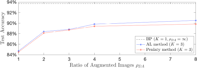
Figure 4: Testing accuracy of ResNet-110 on CIFAR-10 using data augmentation.

To further justify our argument, we show in Figure 4 the test accuracy of decoupled ResNet-110 on CIFAR-10 dataset, where different ratios of augmented images $\rho_{\textnormal{DA}}$ (i.e., the number of synthetically modified images to that of real images) is utilized during training and $\rho_{\textnormal{DA}}=\infty$ denotes the data augmentation containing random operations. It can be observed that, as $\rho_{\textnormal{DA}}$ is increased, the accuracy gap between the traditional layer-serial training approach and the proposed layer-parallel training methods is tending to close. However, the memory requirements for storing all the augmented images and their corresponding auxiliary variables blow up even for moderate values of $\rho_{\textnormal{DA}}$, which could be unaffordable in practical scenarios.

To enable the use of random data augmentation during the layer-parallel training process, we propose a novel joint learning framework that allows trade-off between storage and recomputation of the external auxiliary variables. We can, for instance, take the example of penalty method. If not specified otherwise, the term auxiliary variables is used to only refer to $\{\lambda_{k}\}_{k=0}^{K-1}$ in what follows. Instead of writing the auxiliary variables directly to the CPU memory after each correction (23) (see the second figure in Table 3), an auxiliary-variable network is trained to learn the mapping between these auxiliary variables by replicating their values at the current iteration (see the third figure in Table 3), that is, for $1\leq k\leq K-1$,

$$\lambda_{k-1}\mapsto\lambda_{k}=\textnormal{AuxNet}^{(\lambda)}_{k-1}(\lambda_{k-1};\theta_{k-1}^{(\lambda)})$$ (25)

or, equivalently, the AuxNet above is trained to solve the following minimization problem with pairs of input-output data obtained from (23)

$$\operatorname*{arg\,min}_{\theta_{k-1}^{(\lambda)}}\big{\lVert}\lambda_{k}-\textnormal{AuxNet}^{(\lambda)}_{k-1}(\lambda_{k-1};\theta_{k-1}^{(\lambda)})\big{\rVert}_{\ell_{2}}^{2}$$ (26)

where $\theta_{k-1}^{(\lambda)}$ denotes the trainable parameters. Notably, in contrast to the classical ResNet (1) that requires a large number of model parameters to guarantee its strong exploration capability for solving complex machine learning tasks, the auxiliary-variable network is constructed to mimic the approximate latent feature (or distilled knowledge) generated from the correction operations (23). This observation motivates us to employ a ResNet-like network with small capacity (Gou et al., 2021) for joint training with the layer-parallel training algorithms established in section 4.1, and the experimental results reported in section 5 validate the effectiveness of our proposed strategy.

As a result, the layer-parallel training strategy through the use of penalty method (i.e., forcing $\kappa_{k}\equiv 0$ during training) and auxiliary-variable networks can be formulated as

at each iteration, which achieves forward, backward, and update unlocking without storing the external auxiliary variables in CPU memory. To the best of our knowledge, this is the first study in the literature of training modern ResNets across real-world datasets that breaks the forward locking in a synchronous fashion (see also Table 1 or Table 2).

It is noteworthy that although the explicit Lagrangian multiplier $\kappa_{k}$ has the same size as the auxiliary variable $\lambda_{k}$ for $1\leq k\leq K-1$, the forward dependency between $\kappa_{k-1}$ and $\kappa_{k}$ is not as straightforward as that of $\lambda_{k-1}$ and $\lambda_{k}$. As such, the remaining of this work will focus on the penalty method, and the design of AuxNet architecture for reproducing the explicit Lagrangian multipliers is left for future investigation.

4.2.1 Non-Intrusive Implementation Details

We summarize our results in algorithm 1 for training modern ResNets across real-world datasets, which can be implemented in a non-intrusive way with respect to the existing network architectures. Besides, we denote by $K=1$ the traditional layer-serial training method. Note that for a single iteration step, the computational time associated with the layer-serial ($K=1$) and layer-parallel ($K>1$) training methods are outlined as follows:

Methods	Data Load	Forward Pass	Backpropagation	Auxiliary Network
Layer-Serial	$T_{d}$	$T_{f}$	$T_{b}$	$0$
Layer-Parallel	$T_{d}$	$\frac{1}{K}T_{f}$	$\frac{1}{K}T_{b}+t_{\psi}$	$t^{(\lambda)}_{f}+t^{(\lambda)}_{b}$

where $T_{d}$ denotes the time cost on data loader, $T_{f}$ $(T_{b})$ the time cost of ResNet executing forward (backward) pass through the conventional layer-serial training approach, $t_{\psi}$ the time of computing intermediate loss functions, $t^{(\lambda)}_{f}+t^{(\lambda)}_{b}$ the computation time executing forward pass and knowledge distillation of AuxNets. As a direct result, the speedup ratio per epoch can be expressed as

$$\rho=\frac{\text{runtime per epoch (layer-serial training)}}{\text{runtime per epoch (layer-parallel training)}}=\frac{1}{\frac{1}{K}\frac{T_{f}+T_{b}}{T_{d}+T_{f}+T_{b}}+\frac{T_{d}+t_{\psi}+t^{(\lambda)}_{f}+t^{(\lambda)}_{b}}{T_{d}+T_{f}+T_{b}}}$$ (27)

where $T_{d}$, $T_{f}$, $T_{b}$, $t_{\psi}$, $t^{(\lambda)}_{f}$ and $t^{(\lambda)}_{b}$ are almost independent of the partition number $K$.

// Initialization.

1 split the baseline ResNet model into $K$ parts to deploy model parallelism;

2 initialize the trainable parameters of ResNets and auxiliary-variable networks;

3 schedule proper learning rates for ResNets and auxiliary-variable networks;

4 use a proper penalty function with an increasing sequence of penalty coefficients;

// Training Process.

5 for $j\leftarrow 1$ to $J$ (number of training epochs) do

       foreach mini-batch sampled from training dataset do

             // forward pass to get auxiliary variables

             for $k\leftarrow 0$ to $K-2$ do

                  $\displaystyle\lambda_{k+1}=\textnormal{AuxNet}_{k}^{(\lambda)}(\lambda_{k};\theta_{k}^{(\lambda)})$

             end for

            // decoupled forward-backward pass on multiple GPUs in parallel

             parfor $k\leftarrow 0$ to $K-1$ do

                   // forward pass with auxiliary variable

                   for $m\leftarrow 0$ to $n-1$ do

                        $\displaystyle X_{kn}^{k}=\lambda_{k},\ X_{kn+m+1}^{k}=X_{kn+m}^{k}+F(X_{kn+m}^{k},W_{kn+m})$

                   end for

                  // backpropagation with synthetic and classification losses

                   for $m\leftarrow n$ to $0$ do

                        $\displaystyle W^{k}_{kn+m}\leftarrow W^{k}_{kn+m}-\eta\bigg{(}(1-\delta)\beta\frac{\partial\psi(X^{k}_{kn+n},\lambda_{k+1})}{\partial W^{k}_{kn+m}}+\delta\frac{\partial\varphi(X_{kn+n}^{k})}{\partial W^{k}_{kn+m}}\bigg{)}$

                   end for

                  

             end for

            // communication across GPUs and local knowledge distillation

             parfor $k\leftarrow 1$ to $K-1$ do

                   $\displaystyle\lambda_{k}\leftarrow\lambda_{k}-\eta\bigg{(}(1-\delta)\beta\frac{\partial\psi(X^{k}_{kn+n},\lambda_{k+1})}{\partial X^{k}_{kn}}+\delta\frac{\partial\varphi(X_{kn+n}^{k})}{\partial X^{k}_{kn}}+\beta\frac{\partial\psi(\lambda_{k},X^{k-1}_{kn})}{\partial\lambda}\bigg{)}$

                   $\displaystyle\theta_{k-1}^{(\lambda)}\leftarrow\operatorname*{arg\,min}\big{\lVert}\lambda_{k}-\textnormal{AuxNet}^{(\lambda)}_{k-1}(\lambda_{k-1};\theta_{k-1}^{(\lambda)})\big{\rVert}_{\ell_{2}}^{2}$

                  

             end for

            

       end foreach

      

end for

Algorithm 1 Layer-parallel Training of ResNet with AuxNet (Penalty Method)

Note that the capacity of AuxNets is much smaller than that of realistic ResNets (He et al., 2016a, b), it is plausible to assume that $T_{f}+T_{b}>t_{\psi}+t^{(\lambda)}_{f}+t^{(\lambda)}_{b}$, which immediately shows speed-up over the traditional layer-serial training method by choosing a sufficient large value of $K$. Moreover, formula (27) also implies that the upper bound of speed-up ratio is given by

$$\rho<\frac{T_{d}+T_{f}+T_{b}}{T_{d}+t_{\psi}+t^{(\lambda)}_{f}+t^{(\lambda)}_{b}}.$$

Remark 1

We remark that a different definition of the speedup ratio has been applied by (Huo et al., 2018b). That is, by terminating the parallel training process once its testing accuracy is comparable to that of layer-serial training method, the speedup can then be defined as the ratio of serial execution time to the parallel execution time. Under such a circumstance, testing accuracy becomes the prerequisite for achieving speedup over the traditional method, and (Belilovsky et al., 2020) obtains higher speedup ratio by replacing the original loss function with artificially designed local loss functions during training.

4.2.2 Recursive Auxiliary-Variable Networks

As can be observed from the third figure in Table 3, the time-consuming ResNet realizes forward unlocking with each of its split parts executing the forward pass in a synchronous fashion, however, its accompanied AuxNet still suffers from the issue of forward locking.

To break the forward dependency between the external auxiliary variables, we propose to recursively employ the AuxNets, i.e., another AuxNet can be applied to remove the forward locking of its previous AuxNet and so forth (see the forth figure in Table 3 for example). As an immediate result, all the external auxiliary variables can be generated from the input mini-batch through a stack of AuxNets with different depths (which is referred to as ReAuxNet), that is, for $1\leq k\leq K-1$,

$$\begin{split}\lambda_{k}&=\textnormal{AuxNet}^{(\lambda)}_{k-1}(\textnormal{AuxNet}^{(\lambda)}_{k-2}(\cdots\textnormal{AuxNet}^{(\lambda)}_{0}(\lambda_{0};\theta_{0}^{(\lambda)})\cdots;\theta_{k-2}^{(\lambda)});\theta_{k-1}^{(\lambda)})\\ &=\textnormal{ReAuxNet}^{(\lambda)}_{k}(X_{0};\xi_{k}^{(\lambda)})\end{split}$$

where $\xi_{k}^{(\lambda)}$ represents the network parameters and $\lambda_{0}=X_{0}$. Accordingly, the decoupled forward pass (19) now takes on the form

$$X_{kn}^{k}=\textnormal{ReAuxNet}^{(\lambda)}_{k}(X_{0};\xi_{k}^{(\lambda)}),\ \ X_{kn+m+1}^{k}=X_{kn+m}^{k}+F(X_{kn+m}^{k},W^{k}_{kn+m}),$$ (28)

for $0\leq k\leq K-1$ and $0\leq m\leq n-1$, while the update rule of ReAuxNet satisfies

$$\begin{split}\xi_{k}^{(\lambda)}\leftarrow\xi_{k}^{(\lambda)}-\eta&\bigg{(}\beta\frac{\partial\psi(\lambda_{k},X^{k-1}_{kn})}{\partial\lambda}+(1-\delta_{k,K-1})\beta\frac{\partial\psi(\lambda_{k+1},X^{k}_{kn+n})}{\partial X^{k}_{kn}}\\ &\ \ +\delta_{k,K-1}\frac{\partial\varphi(X_{kn+n}^{k})}{\partial X^{k}_{kn}}\bigg{)}\frac{\partial\textnormal{ReAuxNet}^{(\lambda)}_{k}(X_{0};\xi_{k}^{(\lambda)})}{\partial\xi_{k}^{(\lambda)}}\end{split}$$ (29)

for $1\leq k\leq K-1$. As a result, the layer-parallel training strategy through the use of penalty method (i.e., $\kappa_{k}\equiv 0$) is now given as below.

Though the resulting layer-parallel training strategy is quite attractive due to its simplicity and ability to achieve forward unlocking in both the ResNet and AuxNets, the depth of ReAuxNet grows as the model is partitioned more finely. As a result, it requires more trainable parameters and thus increases the task difficulty for training large ResNets with fine-partitioned stages (see the forth figure in Table 3 for example). On the other hand, an interesting observation is that by forcing the first split parts of all ReAuxNets to have the same trainable parameters, the network structure depicted in the forth figure of Table 3 degenerates to that of the third one, which effectively reduces the total number of network parameters. Therefore, model compression through the use of shared weights is one potential solution to tackle this issue and is left for future investigation.

5 Experiment

To demonstrate the effectiveness and efficiency of our proposed strategy against the most commonly used BP approach and other compared methods, we conduct experiments using the benchmark ResNets (He et al., 2016a) and WideResNet (Zagoruyko and Komodakis, 2016) on CIFAR-10, CIFAR-100, and ImageNet datasets (Krizhevsky et al., 2009, 2012). All our experiments are implemented in Pytorch 1.4 (Paszke et al., 2019) using the multiprocessing library with NCCL backends. The ResNets, together with their accompanied AuxNets, are first split into $K$ pieces of stacked building blocks and then distributed on $K$ independent GPUs (Tesla-V100), where the standard data augmentation techniques, e.g., random crop and flip, are employed during the entire training procedure.

As a preliminary study, we consider the penalty method presented in algorithm 1 and report the training loss, testing accuracy, constraint violation, and speedup ratio. It is noteworthy that in contrast to the regime discussed in remark 1, our definition of speedup ratio is given by (27) and is widely adopted in the parallel computing community (Li et al., 2020).

5.1 ResNet-110 on CIFAR-10 Dataset

To begin with, we consider the benchmark ResNet-110 (He et al., 2016b) on CIFAR-10 dataset (Krizhevsky et al., 2009), where the network architecture is constructed as that described in (He et al., 2016a) and the total number of trainable parameters is around 1.7 million. Models are trained on the 50k training images with a batch size of 128 for 300 epochs, which are then evaluated on the 10k testing images. The initial learning rate of stochastic gradient descent optimizer is set to $0.1$, and then decreases according to a cosine schedule (Loshchilov and Hutter, 2016). The auxiliary variables are perturbed by the Gaussian noise with small variance to prevent from overfitting. If not specified, the penalty coefficient is set to $\beta=10^{5}$ in what follows.

5.1.1 Auxiliary-Variable Network Design

Recall that the AuxNet is designed to mimic the feature maps that generate from the baseline ResNet-110 of different depths, hence a straightforward choice is to employ the original ResNet-110 as our AuxNet. As can be seen from Table 5, the testing accuracy of such a setting is almost the same as the standard BP method, but the additional communication overheads would hamper the speedup ratio.

	ResNet-110	AuxNet for Decoupled ResNet-110 $(K=3)$
		ResNet-110	ResNet-54	ResNet-32	ResNet-20
Test Acc.	93.7$\%$	93.5$\%$	93.0$\%$	92.8$\%$	92.5$\%$
Speedup	-	0.71	1.10	1.30	1.45

Table 5: Testing accuracy and speedup of decoupled ResNet-110 on CIFAR-10, where the AuxNet with different capacities is employed for the joint training framework.

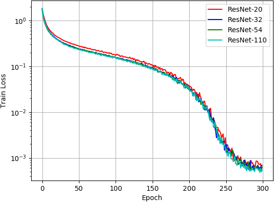
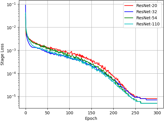
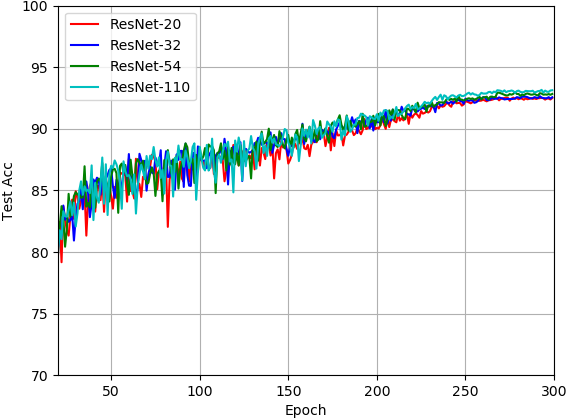
Figure 5: Learning curves of training loss, constraint violation, and test accuracy for decoupled ResNet-110 ($K=3$) on CIFAR-10, where different AuxNets are employed.

On the other hand, the AuxNet is not proposed to solve the classification task, which allows us to reduce its network capacity and further accelerates the training process. As shown in Table 5, the speedup ratio increases as the model capacity of AuxNet declines, while the testing accuracy still remains comparable to the standard BP method (see also Figure 5). To further validate the effectiveness of low-capacity auxiliary-variable network for fulfilling the joint learning task, we employ the ResNet-20 as the AuxNet and conduct experiments using ResNet-32, ResNet-54, and ResNet-110 on CIFAR-10 dataset. The experimental results are reported in Table 6, which shows that our method can boost the training speed of various ResNets while maintain a comparable testing accuracy.

		ResNet-110	ResNet-54	ResNet-32
Layer-Serial	Test Acc.	93.7$\%$	93.3$\%$	92.6$\%$
Layer-Parallel	Test Acc.	92.5$\%$	92.0$\%$	91.3$\%$
	Speedup	1.45	1.18	1.01

Table 6: Testing accuracy and speedup of different ResNets on CIFAR-10, where ResNet- 20 is employed as the AuxNet for decoupled training ($K=3$).

5.1.2 Stage Number and Penalty Coefficient

To further accelerate the network training procedure, we divide the baseline ResNet-110 into $K=4$ stages and summarize the experimental results in Table 7. As the number of decoupled stages grows, the speedup ratio increases but the testing performance of trained model degenerates. This is because that more auxiliary variables and communication overheads are involved as the model is partitioned more finely, making the learning task harder to solve while inducing additional constraint violations. In other words, the increasing number of decoupled stages generally companies with a slight drop in performance. Under such circumstances, a wise strategy for scheduling the penalty coefficient is of crucial importance in order to force the minima of algorithm 1 close to the feasible region of our original problem (1).

	$K=1$	$K=2$	$K=3$	$K=4$
Test Acc.	93.7$\%$	92.8$\%$	92.5$\%$	91.8$\%$
Speedup	-	1.26	1.45	1.68

Table 7: Testing accuracy and speedup of ResNet-110 with different values ($K$) of parallel stages on CIFAR-10, where the ResNet-20 is employed as AuxNet.

Next, we conduct experiments for the decoupled training of ResNet-110 with different values of penalty coefficient. As can be seen from Figure 6, even with the use of different penalty coefficients, the learning curves of the training loss have similar behaviours, i.e., all the optimization problems can be well-solved. However, training with a small penalty coefficient $\beta=10^{3}$ over-explores the infeasible region, which prematurely converges into an infeasible solution that leads to performance degradation (see Table 8). On the contrary, in the case of a very large penalty coefficient, our proposed method may converge just after the feasibility is guaranteed, and hence fails to explore the infeasible region properly. To conclude, the value of penalty coefficient determines the superiority between the classification term and penalty term in the objective loss function (8), and a penalty coefficient that is too small or too large will result in performance degradation.

	$\beta=10^{3}$	$\beta=10^{4}$	$\beta=10^{5}$	$\beta=10^{6}$
Test Acc.	37.8$\%$	91.7$\%$	92.5$\%$	92.3$\%$

Table 8: Testing accuracy of decoupled ResNet-110 ($K=3$) using different penalty coefficients on CIFAR-10, where the ResNet-20 is employed as the AuxNet.

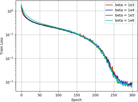
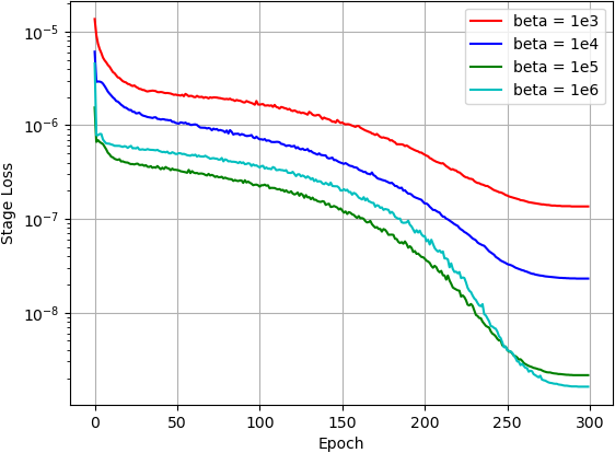
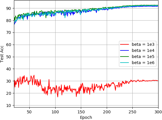
Figure 6: Learning curves of the training loss, penalty loss, and testing accuracy for decoupled ResNet-110 on CIFAR-10 $(K=3)$, where different values of $\beta$ are used.

5.1.3 Comparison to Other Methods

We then compare our joint learning approach with other representative methods from literature for solving the image classification task (1) across CIFAR-10 dataset. Recall from Table 2 or Table 1 that the algorithmic locking issues of BP are not addressed by neither PipeDream nor Gpipe while the loss function of DGL methods is not consistent with the original learning task, the comparison is therefore made against the straight-forward implementation of penalty method without using data augmentation (Gotmare et al., 2018), FR (Huo et al., 2018a), DDG (Huo et al., 2018b) and BP (He et al., 2016a). We follow exactly the same setup from (Huo et al., 2018b, a) and report the experimental results in Table 9. It is noteworthy that in contrast to the definition of speedup ratio applied in (Huo et al., 2018b), we adopt the more commonly used definition (27) for measuring the speed gain of parallel processing. Under such a circumstance, both DDG and FR show no speedup over the traditional layer-serial method (see Table 9), which is caused by the time-consuming communication overheads per epoch during training. On the other hand, it can be concluded from Table 9 that enabling the use of data augmentation at training time can significantly improves the performance of naive penalty method, which validates the effectiveness and efficiency of AuxNet for fulfilling the joint learning task. Besides, our method is also comparable to that of FR and DDG in terms of testing accuracy.

	BP	Penalty	DDG	FR	Our Method
Test Acc.	93.7$\%$	84.5$\%$	93.4$\%$	93.8$\%$	92.5$\%$
Speedup	-	1.56	0.81	0.63	1.45

Table 9: Testing accuracy and speedup of various ResNet training strategies on CIFAR-10 dataset, where the baseline ResNet-110 is decoupled into $K=3$ pieces.

5.2 Large-Scale Experiments

Note that, in contrast to the conventional auxiliary-variable methods, a key advantage of our strategy is that the algorithmic locking problems can be removed without explicitly storing the external auxiliary variables. This allows us to conduct experiments on large-scale datasets, and the results further demostrate the effectiveness of our methods.

More specifically, we first work with WideResNet-40-10 (Zagoruyko and Komodakis, 2016) for CIFAR-100 dataset (Krizhevsky et al., 2009), where the feature map is roughly 10 times larger than that of ResNet-110 on CIFAR-10. Accordingly, the size of auxiliary variables increases significantly as the neural network gets wider, resulting in a very large-scale optimization problem that is challenging to solve. The training starts with a learning rate of $0.1$, which then decays according to the cosine schedule (Loshchilov and Hutter, 2016) for 200 epochs. The initial penalty coefficient is set to $10^{6}$, and is multiplied by $10$ after 50 epochs. As can be seen from Table 10, our joint learning framework still works well under such a challenging scenario, achieving notable speedup with an acceptable drop of testing accuracy.

	WideResNet-40-10	AuxNet for Decoupled WideResNet-40-10
		WideResNet-28-10		WideResNet-16-10
Test Acc.	81.4$\%$	80.1$\%$		79.0$\%$
Speedup	-	1.16		1.53

Table 10: Testing accuracy and speedup of decoupled WideResNet-40-10 on CIFAR-100, in which the AuxNet with different capacities is employed and $K=3$.

Next, we consider the more challenging ImageNet dataset (Krizhevsky et al., 2012) and compare the proposed training approach with other representative methods. More specifically, the ResNet-50 (He et al., 2016b) is chosen as the baseline model, together with ResNet-18 being employed as our AuxNet. All models are split across $K=2$ independent GPUs, and the training terminates after 90 epochs. The initial learning rate is $0.1$ and is divided by 10 every 30 epochs, while the penalty coefficient is set to $\beta=10^{8}$. The experimental results are displayed in Table 11, where all methods except the FR achieve speedup over the standard BP but suffer more or less from the drop of accuracy. This is because that the speedup ratio is defined by (27) rather than that in (Huo et al., 2018b, a). Notably, our method outperforms the other parallel training strategies in terms of test accuracy while the speedup is comparable to that of Sync-DGL.

	BP	FR	Sync-DGL	Our Method
Test Acc.	76.5$\%$	74.4$\%$	73.5$\%$	74.6$\%$
Speedup	-	0.70	1.44	1.40

Table 11: Testing accuracy and speedup of various methods on ImageNet dataset, in which the ResNet-50 is decoupled into $K=2$ pieces and ResNet-18 is used as AuxNet.

6 Concluding Remarks

In this paper, a novel joint learning framework is proposed for the distributed training of modern ResNets across real-world datasets, which fully decouples the conventional forward-backward training process through the employment of low-capacity auxiliary-variable networks. The similarity of training ResNets to the terminal control of neural ODEs motivates us to first utilize the penalty and AL methods for breaking the algorithmic locking in the continuous-time sense, and then to apply a consistent discretization scheme to achieve forward, backward, and update unlocking. Moreover, by trading off storage and recomputation of the external auxiliary variables, the proposed AuxNet enables the use of data augmentation during training, which is of great significance for improving the performance of trained models but not addressed by the existing auxiliary-variable methods. Experimental results are reported to validate the effectiveness and efficiency of our method. For future work, we plan to explore the viability of recursive AuxNets and design efficient AuxNets for reproducing the explicit Lagrangian multipliers.

Appendix

Appendix A Layer-Serial Training

Note that by defining $\displaystyle P_{\ell+1}=\frac{\partial\varphi(X_{L})}{\partial X_{\ell+1}}$ for $0\leq\ell\leq L-1$, scheme (3) can be rewritten as

$$W_{\ell}\leftarrow W_{\ell}-\eta P_{\ell+1}\frac{\partial F(X_{\ell},W_{\ell})}{\partial W},\qquad 0\leq\ell\leq L-1,$$ (30)

where ${\{P_{\ell+1}\}_{\ell=0}^{L-1}}$ satisfy a backward dynamic that captures the loss changes with respect to the hidden activations, i.e.,

$$P_{\ell}=P_{\ell+1}+P_{\ell+1}\frac{\partial F(X_{\ell},W_{\ell})}{\partial X},\qquad P_{L}=\frac{\partial\varphi(X_{L})}{\partial X_{L}}.$$ (31)

Such a sequential propagation of error gradient is also known as the backward locking (Jaderberg et al., 2017), preventing all layers of the network from updating until their dependent layers have executed the backward computation (31).

Consequently, the layer-serial BP algorithm (3) is handled by formulae (31) and (30). Or, to put it differently, the training process of ResNets at each epoch is performed through the repeated execution of

which can be time-consuming as it is common to see neural networks with hundreds or even thousands of layers.

Appendix B Time-Serial Training

By introducing the Lagrange functional with multiplier $p_{t}$ (Nocedal and Wright, 2006), solving the constrained optimization problem (2) is equivalent to finding saddle points of the following Lagrange functional without constraints

$$\begin{split}\mathcal{L}(x_{t},w_{t},p_{t})&=\varphi(x_{1})+\int_{0}^{1}p_{t}\left(f(x_{t},w_{t})-\dot{x}_{t}\right)dt\\ &=\varphi(x_{1})-p_{1}x_{1}+p_{0}x_{0}+\int_{0}^{1}p_{t}f(x_{t},w_{t})+\dot{p}_{t}x_{t}\,dt.\end{split}$$

and the variation in functional $\mathcal{L}(x_{t},w_{t},p_{t})$ corresponding to a variation $\delta w$ in the control variable $w_{t}$ takes on the form (Liberzon, 2011)

$$\delta\mathcal{L}=\bigg{[}\frac{\partial\varphi(x_{1})}{\partial x}-p_{1}\bigg{]}\delta x+\int_{0}^{1}\bigg{(}p_{t}\frac{\partial f(x_{t},w_{t})}{\partial x}+\dot{p}_{t}\bigg{)}\delta x+\bigg{(}p_{t}\frac{\partial f(x_{t},w_{t})}{\partial w}\bigg{)}\delta w\,dt,$$

which leads to the necessary conditions for $w_{t}=w_{t}^{*}$ to be the extremal of $\mathcal{L}(x_{t},w_{t},p_{t})$, i.e.,

$$dx_{t}^{*}=f(x_{t}^{*},w_{t}^{*})dt, x_{0}^{*}=S(y), (\textnormal{state equation})$$

$$dp_{t}^{*}=-p_{t}^{*}\frac{\partial f(x_{t}^{*},w_{t}^{*})}{\partial x}dt, p_{1}^{*}=\frac{\partial\varphi(x_{1}^{*})}{\partial x}, (\textnormal{adjoint equation})$$

$$p_{t}^{*}\frac{\partial f(x_{t}^{*},w_{t}^{*})}{\partial w}=0, \textnormal{for}\ 0\leq t\leq 1. (\textnormal{optimality condition})$$

However, directly solving this optimality system is computationally infeasible, a gradient-based iterative approach with step size $\eta>0$ is typically used, e.g.,

$$dx_{t}=f(x_{t},w_{t})dt, x_{0}=S(y), (\textnormal{forward pass})$$ (32a)

$$dp_{t}=-p_{t}\frac{\partial f(x_{t},w_{t})}{\partial x}dt, p_{1}=\frac{\partial\varphi(x_{1})}{\partial x}, (\textnormal{backward gradient propagation})$$ (32b)

$$w_{t}\leftarrow w_{t}-\eta p_{t}\frac{\partial f(x_{t},w_{t})}{\partial w}, \textnormal{for}\ 0\leq t\leq 1, (\textnormal{parameter updates})$$ (32c)

which is consistent with the layer-serial training process through forward-backward propagation, i.e., (1), (31) and (30), by taking the limit as $L\to\infty$ (Li et al., 2017). In other words, the classic BP scheme (3) for solving problem (1) can be recovered from (4) and (5) after employing the stable discretization schemes (31) and (30).

Appendix C Time-Parallel Training (Augmented Lagrangian Method)

Recall that the augmented Lagrangian functional

$$\begin{split}&\mathcal{L}_{\textnormal{AL}}(x_{t}^{k},p_{t}^{k},w^{k}_{t},\lambda_{k},\kappa_{k})=\mathcal{L}_{\textnormal{P}}(x_{t}^{k},p_{t}^{k},w^{k}_{t},\lambda_{k})-\sum_{k=0}^{K-1}\kappa_{k}(\lambda_{k}-x^{k-1}_{s_{k}^{-}})\\ =\ &\varphi(x^{K-1}_{s_{K}^{-}})+\sum_{k=0}^{K-1}\bigg{(}\beta\psi(\lambda_{k},x^{k-1}_{s_{k}^{-}})-\kappa_{k}(\lambda_{k}-x^{k-1}_{s_{k}^{-}})+\int_{s_{k}}^{s_{k+1}}p^{k}_{t}\big{(}f(x_{t}^{k},w^{k}_{t})-\dot{x}_{t}^{k}\big{)}dt\bigg{)}\\ =\ &\varphi(x^{K-1}_{s_{K}^{-}})+\sum_{k=0}^{K-1}\bigg{(}\beta\psi(\lambda_{k},x^{k-1}_{s_{k}^{-}})-\kappa_{k}(\lambda_{k}-x^{k-1}_{s_{k}^{-}})+\int_{s_{k}}^{s_{k+1}}p^{k}_{t}f(x_{t}^{k},w^{k}_{t})+\dot{p}_{t}^{k}x_{t}^{k}\,dt\\ &\qquad\qquad\qquad\ \ \ \ \ -p^{k}_{s_{k+1}^{-}}x^{k}_{s_{k+1}^{-}}+p^{k}_{s_{k}^{+}}\lambda_{k}\bigg{)}\end{split}$$

can be decomposed as parts involving $x_{t}^{K-1}$ and $\{x_{t}^{k}\}_{k=0}^{K-2}$, i.e.,

$$\varphi(x^{K-1}_{s_{K}^{-}})-p_{s_{K}^{-}}^{K-1}x_{s_{K}^{-}}^{K-1}+p_{s_{K-1}^{+}}^{K-1}\lambda_{K-1}+\int_{s_{K-1}}^{s_{K}}p_{t}^{K-1}f(x_{t}^{K-1},w^{K-1}_{t})+\dot{p}_{t}^{K-1}x_{t}^{K-1}\,dt,$$

and

$$\sum_{k=0}^{K-2}\beta\psi(\lambda_{k+1},x^{k}_{s_{k+1}^{-}})+(\kappa_{k+1}-p^{k}_{s_{k+1}^{-}})x^{k}_{s_{k+1}^{-}}+p^{k}_{s_{k}^{+}}\lambda_{k}+\int_{s_{k}}^{s_{k+1}}p_{t}^{k}f(x_{t}^{k},w^{k}_{t})+\dot{p}_{t}^{k}x_{t}^{k}\,dt-\kappa_{k+1}\lambda_{k+1}$$

respectively. Then the variation in $\mathcal{L}_{\textnormal{AL}}(x_{t}^{k},p_{t}^{k},w^{k}_{t},\lambda_{k},\kappa_{k})$ corresponding to a variation $\delta w_{t}^{k}$ in control $w^{k}_{t}$ takes on the form

$$\begin{split}\delta\mathcal{L}_{\textnormal{AL}}&=\Bigg{(}\frac{\partial\varphi(x^{K-1}_{s_{K}^{-}})}{\partial x}-p_{s_{K}^{-}}^{K-1}\Bigg{)}\delta x^{K-1}+\int_{s_{K-1}}^{s_{K}}\Bigg{(}p_{t}^{K-1}\frac{\partial f(x_{t}^{K-1},w^{K-1}_{t})}{\partial x}+\dot{p}_{t}^{K-1}\Bigg{)}\delta x^{K-1}\,dt\\ &+\sum_{k=0}^{K-2}\Bigg{(}\beta\frac{\partial\psi(\lambda_{k+1},x^{k}_{s_{k+1}^{-}})}{\partial x}+\kappa_{k+1}-p_{s_{k+1}^{-}}^{k}\Bigg{)}\delta x^{k}+\int_{s_{k}}^{s_{k+1}}\bigg{(}p_{t}^{k}\frac{\partial f(x_{t}^{k},w^{k}_{t})}{\partial x}+\dot{p}_{t}^{k}\bigg{)}\delta x^{k}\,dt,\end{split}$$

which implies that the adjoint (or co-state) variable $p_{t}^{k}$ satisfies the backward differential equations (14) (Liberzon, 2011), i.e., for any $0\leq k\leq K-1$,

$$\begin{array}[]{l}\displaystyle dp_{t}^{k}=-p_{t}^{k}\frac{\partial f(x_{t}^{k},w^{k}_{t})}{\partial x}dt\ \ \textnormal{on}\ [s_{k},s_{k+1}),\\ \displaystyle p^{k}_{s_{k+1}^{-}}=\left(1-\delta_{k,K-1}\right)\left(\beta\frac{\partial\psi(\lambda_{k+1},x^{k}_{s_{k+1}^{-}})}{\partial x}+\kappa_{k+1}\right)+\delta_{k,K-1}\,\frac{\partial\varphi(x^{k}_{s_{k+1}^{-}})}{\partial x}.\end{array}$$

On the other hand, it can be easily deduced that the control updates satisfy

$$w_{t}^{k}\leftarrow w_{t}^{k}-\eta p_{t}^{k}\frac{\partial f(x_{t}^{k},w^{k}_{t})}{\partial w}\ \ \ \textnormal{on}\ [s_{k},s_{k+1}]$$

for $0\leq k\leq K-1$, and the correction of auxiliary variables now takes on the form

$$\lambda_{0}\equiv x_{0}\ \ \ \textnormal{and}\ \ \ \lambda_{k}\leftarrow\lambda_{k}-\eta\Bigg{(}\beta\frac{\partial\psi(\lambda_{k},x^{k-1}_{s_{k}^{-}})}{\partial\lambda}+p^{k}_{s_{k}^{+}}-\kappa_{k}\Bigg{)}\ \ \textnormal{for}\ 1\leq k\leq K-1.$$

Obviously, by forcing the Lagrangian multiplier $\kappa_{k}\equiv 0$ for all $0\leq k\leq K-1$, the augmented Lagrangian method degenerates to the standard penalty approach.

References

- Belilovsky et al. (2019) Eugene Belilovsky, Michael Eickenberg, and Edouard Oyallon. Greedy layerwise learning can scale to imagenet. In International conference on machine learning, pages 583–593. PMLR, 2019.
- Belilovsky et al. (2020) Eugene Belilovsky, Michael Eickenberg, and Edouard Oyallon. Decoupled greedy learning of cnns. In International Conference on Machine Learning, pages 736–745. PMLR, 2020.
- Belilovsky et al. (2021) Eugene Belilovsky, Louis Leconte, Lucas Caccia, Michael Eickenberg, and Edouard Oyallon. Decoupled greedy learning of cnns for synchronous and asynchronous distributed learning. arXiv preprint arXiv:2106.06401, 2021.
- Bottou (2010) Léon Bottou. Large-scale machine learning with stochastic gradient descent. In Proceedings of COMPSTAT’2010, pages 177–186. Springer, 2010.
- Brunton et al. (2020) Steven L Brunton, Bernd R Noack, and Petros Koumoutsakos. Machine learning for fluid mechanics. Annual Review of Fluid Mechanics, 52:477–508, 2020.
- Carraro et al. (2015) Thomas Carraro, Michael Geiger, SK Rorkel, and Rolf Rannacher. Multiple Shooting and Time Domain Decomposition Methods. Springer, 2015.
- Carreira-Perpinan and Wang (2014) Miguel Carreira-Perpinan and Weiran Wang. Distributed optimization of deeply nested systems. In Artificial Intelligence and Statistics, pages 10–19. PMLR, 2014.
- Chen et al. (2018) Ricky Chen, Yulia Rubanova, Jesse Bettencourt, and David Duvenaud. Neural ordinary differential equations. In Advances in Neural Information Processing Systems, 2018.
- Choromanska et al. (2018) Anna Choromanska, Benjamin Cowen, Sadhana Kumaravel, Ronny Luss, Mattia Rigotti, Irina Rish, Brian Kingsbury, Paolo DiAchille, Viatcheslav Gurev, Ravi Tejwani, et al. Beyond backprop: Online alternating minimization with auxiliary variables. arXiv preprint arXiv:1806.09077, 2018.
- Dean et al. (2012) Jeffrey Dean, Greg Corrado, Rajat Monga, Kai Chen, Matthieu Devin, Mark Mao, Marc’aurelio Ranzato, Andrew Senior, Paul Tucker, Ke Yang, et al. Large scale distributed deep networks. In Advances in neural information processing systems, pages 1223–1231, 2012.
- E (2017) Weinan E. A proposal on machine learning via dynamical systems. Communications in Mathematics and Statistics, 5(1):1–11, 2017.
- Gnther et al. (2020) Stefanie Gnther, Lars Ruthotto, Jacob B Schroder, Eric C Cyr, and Nicolas R Gauger. Layer-parallel training of deep residual neural networks. SIAM Journal on Mathematics of Data Science, 2(1):1–23, 2020.
- Gholami et al. (2019) Amir Gholami, Kurt Keutzer, and George Biros. Anode: Unconditionally accurate memory-efficient gradients for neural odes. arXiv preprint arXiv:1902.10298, 2019.
- Gotmare et al. (2018) Akhilesh Gotmare, Valentin Thomas, Johanni Brea, and Martin Jaggi. Decoupling backpropagation using constrained optimization methods. 2018.
- Gotschel and Minion (2019) SEBASTIAN Gotschel and Michael L Minion. An efficient parallel-in-time method for optimization with parabolic pdes. SIAM Journal on Scientific Computing, 41(6):C603–C626, 2019.
- Gou et al. (2021) Jianping Gou, Baosheng Yu, Stephen J Maybank, and Dacheng Tao. Knowledge distillation: A survey. International Journal of Computer Vision, 129(6):1789–1819, 2021.
- Gustafson (1988) John L Gustafson. Reevaluating amdahl’s law. Communications of the ACM, 31(5):532–533, 1988.
- Haber and Ruthotto (2017) Eldad Haber and Lars Ruthotto. Stable architectures for deep neural networks. Inverse problems, 34(1):014004, 2017.
- Haber et al. (2018) Eldad Haber, Lars Ruthotto, Elliot Holtham, and Seong-Hwan Jun. Learning across scales—multiscale methods for convolution neural networks. In Thirty-Second AAAI Conference on Artificial Intelligence, 2018.
- Harlap et al. (2018) Aaron Harlap, Deepak Narayanan, Amar Phanishayee, Vivek Seshadri, Nikhil Devanur, Greg Ganger, and Phil Gibbons. Pipedream: Fast and efficient pipeline parallel dnn training. arXiv preprint arXiv:1806.03377, 2018.
- He et al. (2016a) Kaiming He, Xiangyu Zhang, Shaoqing Ren, and Jian Sun. Deep residual learning for image recognition. In Proceedings of the IEEE conference on computer vision and pattern recognition, pages 770–778, 2016a.
- He et al. (2016b) Kaiming He, Xiangyu Zhang, Shaoqing Ren, and Jian Sun. Identity mappings in deep residual networks. In European Conference on Computer Vision, pages 630–645. Springer, 2016b.
- Hecht-Nielsen (1992) Robert Hecht-Nielsen. Theory of the backpropagation neural network. In Neural networks for perception, pages 65–93. Elsevier, 1992.
- Huang et al. (2019) Yanping Huang, Youlong Cheng, Ankur Bapna, Orhan Firat, Dehao Chen, Mia Chen, HyoukJoong Lee, Jiquan Ngiam, Quoc V Le, Yonghui Wu, et al. Gpipe: Efficient training of giant neural networks using pipeline parallelism. In Advances in Neural Information Processing Systems, pages 103–112, 2019.
- Huo et al. (2018a) Zhouyuan Huo, Bin Gu, and Heng Huang. Training neural networks using features replay. arXiv preprint arXiv:1807.04511, 2018a.
- Huo et al. (2018b) Zhouyuan Huo, Bin Gu, Qian Yang, and Heng Huang. Decoupled parallel backpropagation with convergence guarantee. arXiv preprint arXiv:1804.10574, 2018b.
- Iandola et al. (2016) Forrest N Iandola, Matthew W Moskewicz, Khalid Ashraf, and Kurt Keutzer. Firecaffe: near-linear acceleration of deep neural network training on compute clusters. In Proceedings of the IEEE Conference on Computer Vision and Pattern Recognition, pages 2592–2600, 2016.
- Jaderberg et al. (2017) Max Jaderberg, Wojciech Marian Czarnecki, Simon Osindero, Oriol Vinyals, Alex Graves, David Silver, and Koray Kavukcuoglu. Decoupled neural interfaces using synthetic gradients. In Proceedings of the 34th International Conference on Machine Learning-Volume 70, pages 1627–1635. JMLR. org, 2017.
- Kirby et al. (2020) Andrew Kirby, Siddharth Samsi, Michael Jones, Albert Reuther, Jeremy Kepner, and Vijay Gadepally. Layer-parallel training with gpu concurrency of deep residual neural networks via nonlinear multigrid. In 2020 IEEE High Performance Extreme Computing Conference (HPEC), pages 1–7. IEEE, 2020.
- Krizhevsky et al. (2009) Alex Krizhevsky, Geoffrey Hinton, et al. Learning multiple layers of features from tiny images. 2009.
- Krizhevsky et al. (2012) Alex Krizhevsky, Ilya Sutskever, and Geoffrey E Hinton. Imagenet classification with deep convolutional neural networks. Advances in neural information processing systems, 25:1097–1105, 2012.
- LeCun et al. (2015) Yann LeCun, Yoshua Bengio, and Geoffrey Hinton. Deep learning. nature, 521(7553):436–444, 2015.
- Li et al. (2020) Jia Li, Mingqing Xiao, Cong Fang, Yue Dai, Chao Xu, and Zhouchen Lin. Training neural networks by lifted proximal operator machines. IEEE Transactions on Pattern Analysis and Machine Intelligence, 2020.
- Li et al. (2017) Qianxiao Li, Long Chen, Cheng Tai, and E Weinan. Maximum principle based algorithms for deep learning. The Journal of Machine Learning Research, 18(1):5998–6026, 2017.
- Lian et al. (2015) Xiangru Lian, Yijun Huang, Yuncheng Li, and Ji Liu. Asynchronous parallel stochastic gradient for nonconvex optimization. Advances in Neural Information Processing Systems, 28:2737–2745, 2015.
- Liberzon (2011) Daniel Liberzon. Calculus of variations and optimal control theory: a concise introduction. Princeton University Press, 2011.
- Loshchilov and Hutter (2016) Ilya Loshchilov and Frank Hutter. Sgdr: Stochastic gradient descent with warm restarts. arXiv preprint arXiv:1608.03983, 2016.
- Löwe et al. (2019) Sindy Löwe, Peter O’Connor, and Bastiaan S Veeling. Putting an end to end-to-end: Gradient-isolated learning of representations. arXiv preprint arXiv:1905.11786, 2019.
- Maday and Turinici (2002) Yvon Maday and Gabriel Turinici. A parareal in time procedure for the control of partial differential equations. Comptes Rendus Mathematique, 335(4):387–392, 2002.
- Marra et al. (2020) Giuseppe Marra, Matteo Tiezzi, Stefano Melacci, Alessandro Betti, Marco Maggini, and Marco Gori. Local propagation in constraint-based neural network. arXiv preprint arXiv:2002.07720, 2020.
- Miyato et al. (2017) Takeru Miyato, Daisuke Okanohara, Shin-ichi Maeda, and Masanori Koyama. Synthetic gradient methods with virtual forward-backward networks. 2017.
- Mostafa et al. (2018) Hesham Mostafa, Vishwajith Ramesh, and Gert Cauwenberghs. Deep supervised learning using local errors. Frontiers in neuroscience, 12:608, 2018.
- Narayanan et al. (2019) Deepak Narayanan, Aaron Harlap, Amar Phanishayee, Vivek Seshadri, Nikhil R Devanur, Gregory R Ganger, Phillip B Gibbons, and Matei Zaharia. Pipedream: generalized pipeline parallelism for dnn training. In Proceedings of the 27th ACM Symposium on Operating Systems Principles, pages 1–15, 2019.
- Narayanan et al. (2021) Deepak Narayanan, Amar Phanishayee, Kaiyu Shi, Xie Chen, and Matei Zaharia. Memory-efficient pipeline-parallel dnn training. In International Conference on Machine Learning, pages 7937–7947. PMLR, 2021.
- Nocedal and Wright (2006) Jorge Nocedal and Stephen Wright. Numerical optimization. Springer Science & Business Media, 2006.
- Nøkland and Eidnes (2019) Arild Nøkland and Lars Hiller Eidnes. Training neural networks with local error signals. In International Conference on Machine Learning, pages 4839–4850. PMLR, 2019.
- Paine et al. (2013) Thomas Paine, Hailin Jin, Jianchao Yang, Zhe Lin, and Thomas Huang. Gpu asynchronous stochastic gradient descent to speed up neural network training. arXiv preprint arXiv:1312.6186, 2013.
- Parpas and Muir (2019) Panos Parpas and Corey Muir. Predict globally, correct locally: Parallel-in-time optimal control of neural networks. arXiv preprint arXiv:1902.02542, 2019.
- Paszke et al. (2019) Adam Paszke, Sam Gross, Francisco Massa, Adam Lerer, James Bradbury, Gregory Chanan, Trevor Killeen, Zeming Lin, Natalia Gimelshein, Luca Antiga, et al. Pytorch: An imperative style, high-performance deep learning library. Advances in neural information processing systems, 32:8026–8037, 2019.
- Pyeon et al. (2020) Myeongjang Pyeon, Jihwan Moon, Taeyoung Hahn, and Gunhee Kim. Sedona: Search for decoupled neural networks toward greedy block-wise learning. In International Conference on Learning Representations, 2020.
- Rumelhart et al. (1985) David E Rumelhart, Geoffrey E Hinton, and Ronald J Williams. Learning internal representations by error propagation. Technical report, California Univ San Diego La Jolla Inst for Cognitive Science, 1985.
- Tanner and Wong (1987) Martin A Tanner and Wing Hung Wong. The calculation of posterior distributions by data augmentation. Journal of the American statistical Association, 82(398):528–540, 1987.
- Taylor et al. (2016) Gavin Taylor, Ryan Burmeister, Zheng Xu, Bharat Singh, Ankit Patel, and Tom Goldstein. Training neural networks without gradients: A scalable admm approach. In International conference on machine learning, pages 2722–2731, 2016.
- Thorpe and van Gennip (2018) Matthew Thorpe and Yves van Gennip. Deep limits of residual neural networks. arXiv preprint arXiv:1810.11741, 2018.
- Wang et al. (2021) Yulin Wang, Zanlin Ni, Shiji Song, Le Yang, and Gao Huang. Revisiting locally supervised learning: an alternative to end-to-end training. arXiv preprint arXiv:2101.10832, 2021.
- Xu et al. (2020) An Xu, Zhouyuan Huo, and Heng Huang. On the acceleration of deep learning model parallelism with staleness. In Proceedings of the IEEE/CVF Conference on Computer Vision and Pattern Recognition, pages 2088–2097, 2020.
- Zagoruyko and Komodakis (2016) Sergey Zagoruyko and Nikos Komodakis. Wide residual networks. arXiv preprint arXiv:1605.07146, 2016.
- Zeng et al. (2018) Jinshan Zeng, Shikang Ouyang, Tim Tsz-Kit Lau, Shaobo Lin, and Yuan Yao. Global convergence in deep learning with variable splitting via the kurdyka-łojasiewicz property. arXiv preprint arXiv:1803.00225, 2018.
- Zeng et al. (2019) Jinshan Zeng, Shao-Bo Lin, and Yuan Yao. A convergence analysis of nonlinearly constrained admm in deep learning. arXiv preprint arXiv:1902.02060, 2019.