Mean-Square Stability And Stabilizability Analyses of LTI Systems Under Spatially Correlated Multiplicative Perturbations

Abstract

In this paper, we first study the robust stability problem for discrete-time linear time-invariant systems under stochastic multiplicative uncertainties. Those uncertainties could be are susceptible to describing transmission errors, packet drops, random delays, and fading phenomena in networked control systems. In its full generality, we assume that the multiplicative uncertainties are diagonally structured, and are allowed to be spatially correlated across different patterns, which differs from previously related work significantly. We derive a necessary and sufficient condition for robust stability in the mean-square sense against such uncertainties. Based on the obtained stability condition, we further investigate the mean-square stabilizability and consensusability problems through two case studies of first-order single- and two-agent systems. The necessary and sufficient conditions to guarantee stabilizability and consensusability are derived, which rely on the unstable system dynamics, and the stochastic uncertainty variances.

1 Introduction

Networked control is widely considered a key enabling and transformative technology for the current- and next-generation engineering systems. Networked control systems differ from conventional feedback systems, in which networks are implemented to perform communications and enable exchange of data. For such systems, as the most important feature, multiple tasks can be executed remotely combining the cyberspace and physical space, which reduces effectively the complexity and the overall cost in designing and implementing the control systems. However, the consequent communication noises and transmission losses over uncertain networks usher in new challenges inevitably. Over the past decade, the stability and performance problems of networked control systems have receive compelling attention from the control community (see, e.g.,[1, 2, 3, 4, 5, 6, 7, 8, 9, 10]). Recent studies in [3, 10] reveal that stochastic multiplicative noises can be used to effectively model network communication uncertainties including the random-delay and data-loss network phenomena. This relevance of multiplicative channel noises to networked control systems results in a direct impetus motivating our study.

Throughout of this paper, the channel uncertainties are modelled as diagonally structured multiplicative perturbations, which consist of static, zero-mean stochastic processes. The current model and theory of networked control, however, are unable to break through one fundamental limitation, that is the communication channel noises must be independent or uncorrelated [3, 4, 11, 8]. In this paper, we concentrate on the correlated stochastic multiplicative uncertainties coping with correlated noises, transmission losses, and a wide range of other channel models. Under this formulation, we may enable to construct a framework to examine the robust stability and performance problems of networked control systems under such uncertainties. Note that the descriptions of uncertainty are different from those in robust control theory [12]. In doing so, we assess the system’s stability and performance using mean-square measures [4, 8].

In this paper, we focus on the mean-square stability and stabilizability problems. In the presence of correlated stochastic multiplicative uncertainties, we seek to develop fundamental necessary and sufficient conditions that guarantee the stabilizability of linear time-invariant (LTI) systems by the output feedback controller in the mean-square sense. We first develop a mean-square stability condition, namely a generalized mean-square small gain theorem capable of coping with correlated stochastic uncertainties. Next, under the obtained generalized mean-square framework, we attempt to solve the corresponding mean-square stabilizability problems. At current stage, a complete solution to the generalized LTI systems are still unavailable. We consider two special but representative low-order systems serving as a case study. The first case is the single-input single-output (SISO) first-order unstable plant. The channels between the plant and the controller are perturbed by correlated stochastic uncertainties. We develop the necessary and sufficient mean-square stabilizability conditions for such plant. We next consider a typical multi-agent system containing only two agents, each of which keeps a first-order dynamics. Then the associated mean-square consensusability condition is derived, linking the unstable pole of the agent and the variances of the uncertainties together.

The notations used throughout of this paper are collected herein. Let $\mathbb{R}^{n}$ and $\mathbb{R}^{m\times n}$ be the space of real vectors and real matrices. For any matrix $A\in\mathbb{R}^{n\times n}$, we denote $\rho(A)$, $A^{\top}$, $A^{\ast}$, $A^{\mathrm{H}}$, $A_{ij}$, and $\operatorname{vec}{(A)}$ as the spectral radius, the transpose, the conjugate, the conjugate and transpose, the $ij$th entry, and the column stack, respectively. Given two matrices $A,~{}B\in\mathbb{R}^{n\times n}$, $A\leq(\geq)B$ implies the Loewner order. $I_{n}\in\mathbb{R}^{n\times n}$ denotes a unit matrix, and we may omit the subscript $n$ if the dimension is apparent in context. $\textbf{1}_{n}\in\mathbb{R}^{n}$ represents the vector with all entries equal to one. $\otimes$ and $\circ$ denote the Kronecker product and Hadamard product. We denote the expectation operator by $\mathbb{E}[\cdot]$. At last, given a LTI stable system $G$, we use $\left\lVert G\right\rVert_{2}$ to represent its $\mathcal{H}_{2}$ norm.

2 Problem Formulation and Preliminaries

For consideration of stability and stabilization problems, we start by the uncertain system depicted in Fig. 1. In this configuration, $G$ represents an open-loop stable discrete-time LTI plant.

Figure 1: The LTI system with the stochastic multiplicative uncertainty.

The uncertainty $\Delta$ here admits a diagonal structure such that

$$\Delta(k)=\mathrm{diag}\left(\Delta_{1}(k),\ldots,\Delta_{m}(k)\right),$$ (1)

and

$$u(k)=\Delta(k)y(k).$$

Note that each component $\Delta_{i}(k),~{}i=1,\ldots,m$ is a zero-mean stochastic process. The signals $d(k)$, $u(k)$, $e(k)$ and $y(k)$ denote the external input, the internal input, the error and the output, respectively.

2.1 Structured Multiplicative Uncertainty

Throughout this paper, given the uncertainty $\Delta$ in (1), we make the following assumptions:

Assumption 1

$\left\{\Delta_{i}(k)\right\}$, $i=1,\ldots,m$ is a white noise with a bounded variance $\mathbb{E}[\Delta_{i}(k)^{2}]\leq\sigma_{i}^{2}.$

Assumption 2

$\left\{\Delta_{i}(k)\right\}$, $i=1,\ldots,m$ is uncorrelated with $\left\{d(k)\right\}$.

Assumption 3

$\left\{\Delta_{i}(k)\right\}$ and $\left\{\Delta_{j}(k)\right\}$ are correlated processes $\forall i,\,j$. Denote by the vector $\eta(k)=\left[\Delta_{1}(k),\,\ldots,\,\Delta_{m}(k)\right]^{\top}$, then

$$\mathbb{E}\left[\eta(k)\eta(k)^{\top}\right]\leq\Pi_{\Delta}.$$

Assumptions 1 and 2 are standard in the earlier studies of classical stochastic systems and networked control systems (see, e.g., [4]). This uncertainty may be used to model state-and input-dependent random noises in the stochastic control setting [13, 14], and the communication errors and losses in networks [3, 6]. The main difference from the previous studies is the existence of allowable correlations among the diagonal components in uncertainty $\Delta$, that is Assumption 3. We aim to break a fundamental limitation with the current model and theory of networked control, that is, the communication channel noises must be independent or uncorrelated. Assumption 3 actually captures a wide range of channel uncertainties such as correlated noises, random delays, and transmission losses over common networks, which could be tackled as correlated stochastic multiplicative uncertainties.

2.2 Mean-Square Stability

Consider the mean-square stability problems for the interconnection in Fig. 1. We first provide the definition of mean-square stability from an input-output perspective as follows (see also [4, 8]).

Definition 1

The system in Fig. 1 is said to be mean-square stable if for any input sequence $\left\{d(k)\right\}$ with bounded variance $\mathbb{E}[d(k)d(k)^{\top}]<\infty$, the variances of the error and output sequences ${e(k)}$, ${y(k)}$ are also bounded, i.e., $\mathbb{E}[e(k)e(k)^{\top}]<\infty$ and $\mathbb{E}[y(k)y(k)^{\top}]<\infty$.

Equivalently, as to the internal stability, we mean that for any bounded initial states of the plant, the variances of these states will converge asymptotically to the zero matrix when $k\rightarrow\infty$. We next provide a namely generalized mean-square small-gain theorem capable of coping with correlated stochastic uncertainties, which will play a pivotal role in our subsequent development.

Theorem 2.1.

Let $G$ be a stable LTI plant, and $\Delta$ be a diagonally structured correlated uncertainty under Assumptions 1-3. Then the system in Fig. 1 is mean-square stable if and only if

$$\rho\left(\mathrm{diag}\left(\mathrm{vec}(\Pi_{\Delta})\right)\,\frac{1}{2\pi}\int_{-\pi}^{\pi}\hat{G}^{\ast}(e^{j\omega})\otimes\hat{G}(e^{j\omega})\mathrm{d}\omega\right)<1.$$ (2)

Proof. Sufficiency. Define the autocorrelation matrix and the power spectral density matrix of $e(k)$ as $R_{e}(l)=\mathbb{E}[e(k)e(k+l)^{\top}]$ and $\Phi_{e}(\omega)=\sum\limits_{l=-\infty}^{\infty}R_{e}(l)e^{-j\omega l}$, then we derive that $R_{e}(l)=R_{u}(l)+R_{d}(l)$ and $\Phi_{e}(\omega)=\Phi_{u}(\omega)+\Phi_{d}(\omega)$. In addition, $R_{u}(l)=\mathbb{E}[\Delta(k)R_{y}(l)\Delta(k+l)^{\top}]$ .

Therefore, the power spectral density matrix of the output $y(k)$ proceeds as

$$\Phi_{y}(\omega) =\hat{G}(e^{j\omega})\Phi_{e}(\omega)\hat{G}^{\mathrm{H}}(e^{j\omega})$$

$$=\hat{G}(e^{j\omega})(\Phi_{u}(\omega)+\Phi_{d}(\omega))\hat{G}^{\mathrm{H}}(e^{j\omega})$$

$$=\hat{G}(e^{j\omega})R_{u}(0)\hat{G}^{\mathrm{H}}(e^{j\omega})+\hat{G}(e^{j\omega})R_{d}(0)\hat{G}^{\mathrm{H}}(e^{j\omega})$$

$$=\hat{G}(e^{j\omega})\mathbb{E}[\Delta(k)R_{y}(0)\Delta(k)^{\top}]\hat{G}^{\mathrm{H}}(e^{j\omega})+\hat{G}(e^{j\omega})R_{d}(0)\hat{G}^{\mathrm{H}}(e^{j\omega}).$$

Hence, the covariance matrix of the output $y(t)$ implied by $R_{y}(0)$ suffices that

$$\quad\,\mathbb{E}[y(k)y(k)^{\top}]=R_{y}(0)=\frac{1}{2\pi}\int_{-\pi}^{\pi}\Phi_{y}(\omega)\mathrm{d}\omega$$

$$=\frac{1}{2\pi}\int_{-\pi}^{\pi}\hat{G}(e^{j\omega})\mathbb{E}[\Delta(k)R_{y}(0)\Delta(k)^{\top}]\hat{G}^{\mathrm{H}}(e^{j\omega})\mathrm{d}\omega$$

$$~{}~{}~{}~{}~{}~{}~{}~{}~{}~{}~{}+\frac{1}{2\pi}\int_{-\pi}^{\pi}\hat{G}(e^{j\omega})R_{d}(0)\hat{G}^{\mathrm{H}}(e^{j\omega})\mathrm{d}\omega$$

$$~{}~{}~{}~{}~{}=\frac{1}{2\pi}\int_{-\pi}^{\pi}\hat{G}(e^{j\omega})\left(\mathbb{E}\left[\eta(k)\eta(k)^{\top}\right]\circ R_{y}(0)\right)\hat{G}^{\mathrm{H}}(e^{j\omega})\mathrm{d}\omega$$

$$~{}~{}~{}~{}~{}~{}~{}~{}~{}~{}~{}+\frac{1}{2\pi}\int_{-\pi}^{\pi}\hat{G}(e^{j\omega})R_{d}(0)\hat{G}^{\mathrm{H}}(e^{j\omega})\mathrm{d}\omega.$$

Denote by $\mathbb{E}\left[\eta(k)\eta(k)^{\top}\right]=\bar{\Pi}_{\Delta}$. After the vectorization of $R_{y}(0)$, we rewrite that

$$\quad\,\mathrm{vec}(R_{y}(0))=\frac{1}{2\pi}\int_{-\pi}^{\pi}\hat{G}^{\ast}(e^{j\omega})\otimes\hat{G}(e^{j\omega})\mathrm{d}\omega\,\mathrm{diag}\left(\mathrm{vec}(\bar{\Pi}_{\Delta})\right)\mathrm{vec}(R_{y}(0))$$

$$~{}~{}~{}~{}~{}~{}~{}~{}~{}~{}~{}~{}~{}~{}~{}~{}~{}~{}~{}~{}~{}~{}~{}~{}+\frac{1}{2\pi}\int_{-\pi}^{\pi}\hat{G}^{\ast}(e^{j\omega})\otimes\hat{G}(e^{j\omega})\mathrm{d}\omega\,\mathrm{vec}(R_{d}(0)).$$

Hence, there exists a unique and finite solution for $\mathrm{vec}(R_{y}(0))$ if and only if $I_{n^{2}}-\frac{1}{2\pi}\int_{-\pi}^{\pi}\hat{G}^{\ast}(e^{j\omega})\otimes\hat{G}(e^{j\omega})\mathrm{d}\omega\,\mathrm{diag}\left(\mathrm{vec}(\bar{\Pi}_{\Delta})\right)$ is invertible. A sufficient condition to guarantee this is that

$$\rho\left(\mathrm{diag}\left(\mathrm{vec}(\bar{\Pi}_{\Delta})\right)\frac{1}{2\pi}\int_{-\pi}^{\pi}\hat{G}^{\ast}(e^{j\omega})\otimes\hat{G}(e^{j\omega})\mathrm{d}\omega\right)<1.$$

Let $\mathcal{P}_{n}\triangleq\{X\geq 0\}$. Define a linear operator $\mathcal{T}_{\bar{\Pi}_{\Delta}}:\mathcal{P}_{n}\mapsto\mathcal{P}_{n}$ such that

$$\mathcal{T}_{\bar{\Pi}_{\Delta}}(X)=\frac{1}{2\pi}\int_{-\pi}^{\pi}\hat{G}(e^{j\omega})\left(\bar{\Pi}_{\Delta}\circ X\right)\hat{G}^{\mathrm{H}}(e^{j\omega})\mathrm{d}\omega.$$

Then, it follows that

$$\rho\left(\mathrm{diag}\left(\mathrm{vec}(\bar{\Pi}_{\Delta})\right)\frac{1}{2\pi}\int_{-\pi}^{\pi}\hat{G}^{\ast}(e^{j\omega})\otimes\hat{G}(e^{j\omega})\mathrm{d}\omega\right)=\rho(\mathcal{T}_{\bar{\Pi}_{\Delta}}).$$

Next, we need to prove $\rho(\mathcal{T}_{\bar{\Pi}_{\Delta}})\leq\rho(\mathcal{T}_{\Pi_{\Delta}})$ when $0\leq\bar{\Pi}_{\Delta}\leq\Pi_{\Delta}$. To establish this inequality, we first need three support lemmas [15, 16].

Lemma 2.2.

If $A$ and $B$ are positive semi-definite (positive definite), then $A\circ B$ is positive semi-definite (positive definite).

Lemma 2.3.

Given a linear operator $\mathcal{T}:\mathcal{P}_{n}\mapsto\mathcal{P}_{n}$, then $\rho(\mathcal{T})$ is an eigenvalue of $\mathcal{T}$ together with an eigenvector $X\in\mathcal{P}_{n},\,X\neq 0$, i.e. $\mathcal{T}(X)=\rho(\mathcal{T})X$.

Lemma 2.4.

Given a linear operator $\mathcal{T}:\mathcal{P}_{n}\mapsto\mathcal{P}_{n}$, the associated Collatz-Wielandt set is defined as $\Omega(\mathcal{T})=\left\{\kappa:\exists X\in\mathcal{P}_{n}\setminus\{0\},\mathcal{T}(X)\geq\kappa X\right\}$. Then, it holds

$\sup\Omega(\mathcal{T})=\rho(\mathcal{T}).$

Consider

$$\mathcal{T}_{\Pi_{\Delta}}(X)-\mathcal{T}_{\bar{\Pi}_{\Delta}}(X)=\frac{1}{2\pi}\int_{-\pi}^{\pi}\hat{G}(e^{j\omega})\left((\Pi_{\Delta}-\bar{\Pi}_{\Delta})\circ X\right)\hat{G}^{\mathrm{H}}(e^{j\omega})\mathrm{d}\omega.$$

Lemma 2.2 and $\Pi_{\Delta}-\bar{\Pi}_{\Delta}\leq 0$ yield that $(\Pi_{\Delta}-\bar{\Pi}_{\Delta})\circ X\geq 0,\forall X\geq 0$, then $\mathcal{T}_{\Pi_{\Delta}}(X)-\mathcal{T}_{\bar{\Pi}_{\Delta}}(X)\geq 0.$ Inspired by invoking Lemma 2.3, there must exist $X_{\rho}\in\mathcal{P}_{n}$ as the eigenvector such that $\mathcal{T}_{\bar{\Pi}_{\Delta}}(X_{\rho})=\rho(\mathcal{T}_{\bar{\Pi}_{\Delta}})X_{\rho}.$ Therefore, it follows that $\rho(\mathcal{T}_{\bar{\Pi}_{\Delta}})X_{\rho}\leq\mathcal{T}_{\Pi_{\Delta}}(X_{\rho})$ and, from Lemma 2.4, $\rho(\mathcal{T}_{\bar{\Pi}_{\Delta}})\in\Omega(\mathcal{T}_{\Pi_{\Delta}})$. Hence, $\rho(\mathcal{T}_{\bar{\Pi}_{\Delta}})\leq\sup\Omega(\mathcal{T}_{\Pi_{\Delta}})=\rho(\mathcal{T}_{\Pi_{\Delta}})$. Finally, a sufficient condition to guarantee the mean-square stability is $\rho(\mathcal{T}_{\Pi_{\Delta}})<1$, so is to (2).

Necessity. Assume that there exists the uncertainty $\hat{\Delta}$ with $\bar{\Pi}_{\hat{\Delta}}\leq\Pi_{\hat{\Delta}}$ such that $\rho\left(\mathcal{T}_{\Pi_{\hat{\Delta}}})\right)\geq 1$. Then by the continuity and the monotonicity proved above, we can always find a uncertainty $\hat{\tilde{\Delta}}$ with $\bar{\Pi}_{\hat{\tilde{\Delta}}}\leq\Pi_{\hat{\Delta}}$ satisfying $\rho(\mathcal{T}_{\bar{\Pi}_{\hat{\tilde{\Delta}}}})=1$, which implies the non-uniqueness of $R_{y}(0)$, and then leads to a contradiction. Thus, $\rho(\mathcal{T}_{\Pi_{\Delta}})<1$ is also necessary, so is to (2). $\blacksquare$

Consider also the uncorrelated uncertainty as a special case.

Assumption 4

$\left\{\Delta_{i}(k)\right\}$ and $\left\{\Delta_{j}(k)\right\}$ are uncorrelated processes $\forall i,\,j$, i.e.,

$\mathbb{E}[\Delta_{i}(k)\Delta_{j}(k)]=0,\;\forall\,i\neq j.$

The following result, herein referred to as the mean-square small-gain theorem, is adapted from [4] (see also [8] and [3] ), which provides a necessary and sufficient condition for mean-square stability subject to uncorrelated uncertainties.

Corollary 1

Let $G$ be a stable LTI plant, and $\Delta$ be a diagonally structured uncorrelated uncertainty under Assumptions 1-2 and 4. Then the system in Fig. 1 is mean-square stable if and only if

$$\rho\left(\mathrm{diag}\left(\sigma_{1}^{2},\cdots,\sigma_{m}^{2}\right)\,H\right)<1,$$ (3)

where

$$H=\begin{bmatrix}\left\lVert G_{11}\right\rVert_{2}^{2}&\cdots&\left\lVert G_{1m}\right\rVert_{2}^{2}\\ \vdots&\ddots&\vdots\\ \left\lVert G_{m1}\right\rVert_{2}^{2}&\cdots&\left\lVert G_{mm}\right\rVert_{2}^{2}\end{bmatrix}.$$ (4)

It is worth noting that Theorem 2.1 can reduce to the result above if the uncertainties change to uncorrelated. We omit the details herein.

3 Main Results

Our ultimate goal is developing mean-square stabilization conditions for general LTI plants using the obtained generalized mean-square small-gain theorem as a coherent technical approach. Nevertheless, compared with the existing results concentrated on the uncorrelated uncertainties (see for example [17] and [8]), the mean-square stabilizability via output feedback under correlated uncertainties proves fundamentally more difficult, which appears to be a nontrivial task and is currently unavailable. In this paper, two low-order systems are chosen serving as a case study. Firstly, a SISO first-order unstable plant has been put into consideration and the communication channels between the plant and the controller are perturbed by multiplicative uncertainties. Next, we turn to resolve the mean-square consensusability problem of the two-agent system. Each agent admits a first-order unstable dynamics. We can also observe that one agent communicates with another through a communication channel perturbed by a multiplicative uncertainty.

3.1 Multiplicative $\&$ Divisive Uncertainties

We focus on the uncertain system depicted in Fig. 2. The nominal plant $P$ represents a SISO first-order system with relative degree $\tau=1$ such that

$$P(z)=\dfrac{1}{z-p_{1}},~{}~{}~{}~{}~{}|p_{1}|>1,$$ (5)

and $\tau=0$ such that

$$~{}~{}~{}~{}~{}P(z)=\dfrac{z-s_{1}}{z-p_{1}},~{}~{}~{}~{}~{}|s_{1}|>1,~{}|p_{1}|>1.$$ (6)

The plants $P(z)$ in (5) and (6) both admit an unstable pole $p_{1}$, whereas the latter contains one nonminimum phase zero $s_{1}$. The uncertainties $\Delta_{1}$ and $\Delta_{2}$ are usually named as the multiplicative and divisive uncertainties, both of which are assumed to be zero-mean stochastic processes.

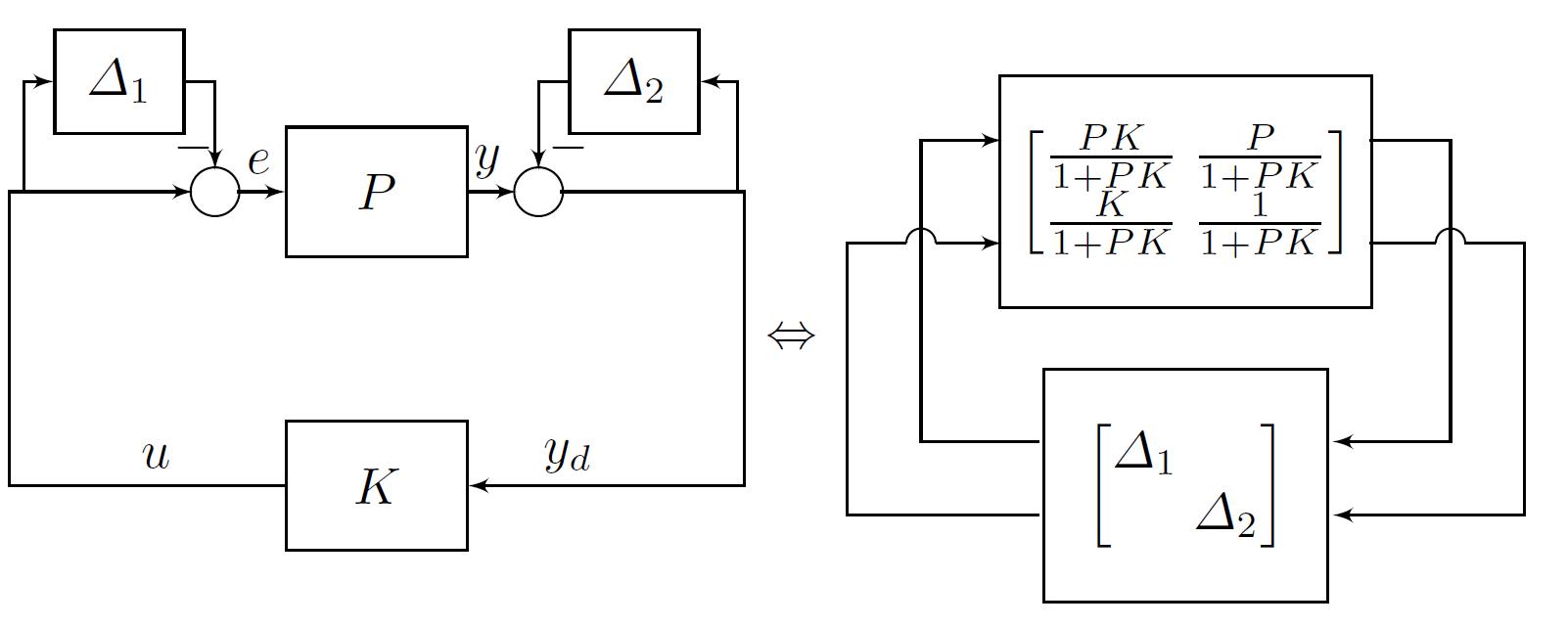
Figure 2: Reshaped loop of system with the correlated uncertainties at plant input and output.

After a linear fractional transformation, we obtain a $G-\Delta$ loop at the right hand side in Fig. 2, where

$$G=\begin{bmatrix}\dfrac{PK}{1+PK}&\dfrac{P}{1+PK}\\ \dfrac{K}{1+PK}&\dfrac{1}{1+PK}\end{bmatrix}$$ (7)

and the uncertainty $\Delta=\mathrm{diag}(\Delta_{1},\Delta_{2})$ satisfies Assumption 1-3 with

$$\Pi_{\Delta}=\begin{bmatrix}\sigma_{1}^{2}&\sigma_{12}\\ \sigma_{12}&\sigma_{2}^{2}\end{bmatrix}.$$ (8)

The following results show that the mean-square stabilizability conditions of the first-order plant under consideration.

Theorem 3.1.

(i) For $P(z)$ in (5), the system in Fig. 2 is mean-square stabilizable if and only if

$$(\sigma_{1}^{2}-2\sigma_{12})(p_{1}^{2}-1)+\sigma_{2}^{2}p_{1}^{2}<1.$$ (9)

(ii) For $P(z)$ in (6), the system in Fig. 2 is mean-square stabilizable if

$$(\sigma_{1}^{2}-2\sigma_{12}+\sigma_{2}^{2})\frac{p_{1}^{2}s_{1}^{2}}{(p_{1}-s_{1})^{2}}+\frac{\sigma_{1}^{2}p_{1}^{2}-2\sigma_{12}s_{1}p_{1}+\sigma_{2}^{2}s_{1}^{2}}{(p_{1}-s_{1})^{2}}<1.$$ (10)

Proof. In light of Theorem 2.1, the system in Fig. 2 is mean-square stabilizable if and only if $\inf_{K:~{}G~{}\mathrm{is~{}stable}}\rho\left(\mathrm{diag}\left(\mathrm{vec}(\Pi_{\Delta})\right)\,\frac{1}{2\pi}\int_{-\pi}^{\pi}\hat{G}^{\ast}(e^{j\omega})\otimes\hat{G}(e^{j\omega})\mathrm{d}\omega\right)\!\!<\!1.$ Specifically, it follows that

$$\!\!\inf_{K:~{}G~{}\mathrm{is~{}stable}}\!\!\!\!\!\!\rho\left(\mathrm{diag}\left(\mathrm{vec}(\Pi_{\Delta})\right)\ \frac{1}{2\pi}\int_{-\pi}^{\pi}\left|\frac{1}{1+P(e^{j\omega})K(e^{j\omega})}\right|^{2}\right.$$

$$~{}~{}~{}~{}~{}~{}~{}~{}~{}~{}~{}~{}~{}~{}~{}~{}~{}~{}~{}~{}~{}~{}\left.\left(\begin{bmatrix}\left|P(e^{j\omega})\right|^{2}\\ P^{\ast}(e^{j\omega})\\ P(e^{j\omega})\\ 1\end{bmatrix}\begin{bmatrix}\left|K(e^{j\omega})\right|^{2}&K^{\ast}(e^{j\omega})&K(e^{j\omega})&1\end{bmatrix}\right)\mathrm{d}\omega\right)\!\!<\!1.$$

Toward the first-order system, it is rather enough to consider only the constant output feedback, i.e., $K=K(e^{j\omega})$. We then have

$$\!\!\inf_{K:~{}G~{}\mathrm{is~{}stable}} \rho\left(\mathrm{diag}\left(\mathrm{vec}(\Pi_{\Delta})\right)\ \frac{1}{2\pi}\int_{-\pi}^{\pi}\left|\frac{1}{1+P(e^{j\omega})K}\right|^{2}\begin{bmatrix}|P(e^{j\omega})|^{2}\\ P^{\ast}(e^{j\omega})\\ P(e^{j\omega})\\ 1\end{bmatrix}\mathrm{d}\omega\begin{bmatrix}K^{2}&K&K&1\end{bmatrix}\right)\!\!<\!1.$$

Apparently, the matrix inside the spectral radius operator is rank-one, which, along with Lemma 2.3, indicates the equality between the spectral radius and the trace of the given matrix. The mean-square stabilizable condition reduces to

$$\!\!\inf_{K:~{}G~{}\mathrm{is~{}stable}}\frac{1}{2\pi}\int_{-\pi}^{\pi}\left|\frac{1}{1+P(e^{j\omega})K}\right|^{2}\times$$

$$\left(\sigma_{1}^{2}|P(e^{j\omega})|^{2}K^{2}+\sigma_{12}(P^{\ast}(e^{j\omega})+P(e^{j\omega}))K+\sigma_{2}^{2}\right)\mathrm{d}\omega<1.$$

Case I: $P(e^{j\omega})=1/(e^{j\omega}-p_{1})$. It is easy to verify that $-1+p_{1}<K<1+p_{1}$. Denote by

$$f_{\mathrm{I}}(K) =\frac{1}{2\pi}\int_{-\pi}^{\pi}\left|\frac{1}{1+\frac{1}{e^{j\omega}-p_{1}}K}\right|^{2}\times$$

$$~{}~{}~{}~{}~{}~{}~{}~{}~{}~{}~{}\left(\sigma_{1}^{2}|\frac{1}{e^{j\omega}-p_{1}}|^{2}K^{2}+\sigma_{12}(\frac{1}{e^{-j\omega}-p_{1}}+\frac{1}{e^{j\omega}-p_{1}})K+\sigma_{2}^{2}\right)\mathrm{d}\omega$$

$$=\frac{1}{1-(p_{1}-K)^{2}}\left((\sigma_{1}^{2}-2\sigma_{12})K^{2}+2\sigma_{2}^{2}p_{1}K+\sigma_{2}^{2}(1-p_{1}^{2})\right).$$

Taking the derivative of $f_{\mathrm{I}}(K)$ with $K$, we have

$$f_{\mathrm{I}}^{\prime}(K)=\frac{2(\sigma_{1}^{2}-2\sigma_{12}+\sigma_{2}^{2})}{(1-(p_{1}-K)^{2})^{2}}\left(p_{1}k^{2}+(1-p_{1}^{2})k\right).$$

Then we obtain $K^{\ast}=p_{1}-1/p_{1}$ such that $f_{\mathrm{I}}^{\prime}(K^{\ast})=0$. Note that $\sigma_{1}^{2}-2\sigma_{12}+\sigma_{2}^{2}>0$. It is evident that $f_{\mathrm{I}}^{\prime}(K)<0$ when $-1+p_{1}<K<K^{\ast}$ and $f_{\mathrm{I}}^{\prime}(K)>0$ when $K^{\ast}<K<1+p_{1}$. Consequently, it can be established that

$$\inf_{K}f_{\mathrm{I}}(K)=f_{\mathrm{I}}(K^{\ast})=(\sigma_{1}^{2}-2\sigma_{12})(p_{1}^{2}-1)+\sigma_{2}^{2}p_{1}^{2},$$

which in turn implies the mean square stabilizability, provided that the condition (9) holds.

Case II: $P(e^{j\omega})=(e^{j\omega}-s_{1})/(e^{j\omega}-p_{1})$. Using Jury stability criterion [18], we first confirm the range of $K$ with

$$\min\{-\frac{1-p_{1}}{1-s_{1}},~{}-\frac{1+p_{1}}{1+s_{1}}\}<K<\max\{-\frac{1-p_{1}}{1-s_{1}},~{}-\frac{1+p_{1}}{1+s_{1}}\}$$

such that the close-loop system $G$ is stable. Next, we consider

$$f_{\mathrm{II}}(K)=\frac{1}{2\pi}\int_{-\pi}^{\pi}\left|\frac{1}{1+\frac{e^{j\omega}-s_{1}}{e^{j\omega}-p_{1}}K}\right|^{2}\times$$

$$~{}~{}~{}~{}~{}~{}~{}~{}~{}\left(\sigma_{1}^{2}|\frac{e^{j\omega}-s_{1}}{e^{j\omega}-p_{1}}|^{2}K^{2}+\sigma_{12}(\frac{e^{-j\omega}-s_{1}}{e^{-j\omega}-p_{1}}+\frac{e^{j\omega}-s_{1}}{e^{j\omega}-p_{1}})K+\sigma_{2}^{2}\right)\mathrm{d}\omega.$$

Let $x=(p_{1}+s_{1}K)/(1+K)\in(-1,1)$ be the stable pole of the close-loop system. We obtain $f_{\mathrm{II}}(K)=g(x),$ where

$$g(x) =\sigma_{1}^{2}\frac{(x-p_{1})^{2}}{(p_{1}-s_{1})^{2}}\frac{1+s_{1}^{2}-2s_{1}x}{1-x^{2}}-2\sigma_{12}\frac{(x-p_{1})(x-s_{1})}{(p_{1}-s_{1})^{2}}\frac{1+s_{1}p_{1}-(s_{1}+p_{1})x}{1-x^{2}}$$

$$~{}~{}~{}~{}~{}~{}~{}~{}~{}~{}+\sigma_{2}^{2}\frac{(x-s_{1})^{2}}{(p_{1}-s_{1})^{2}}\frac{1+p_{1}^{2}-2p_{1}x}{1-x^{2}}.$$

The condition in (10) hence can be established through letting $g(0)<1$. $\blacksquare$

Theorem 3.1 provides a complete solution to the mean-square stabilizability problem in the first-order case against the multiplicative and divisive stochastic uncertainties simultaneously. It is important to note that for the minimum phase plant (5), Theorem 3.1, (9) shows that the mean-square stabilizability condition becomes proportionally more demanding as the variances $\sigma_{1}^{2},~{}\sigma_{2}^{2}$ increase. Also, the distance between the unstable pole $p_{1}$ and the unit circle, as a measure of the system’s instability, plays a central role in the mean-square stabilization. As to the nonminimum phase plant (6), it is clear from (10) that the unstable pole $p_{1}$ and nonminimum phase zero $s_{1}$ coupled together codetermine the mean-square stabilizability condition. Especially when the pole and zero are getting close to each other, it is rather difficult to satisfy the stabilization condition. Note that the influence of the correlation pattern $\sigma_{12}$ in stabilization has been demonstrated clearly in (9) and (10). In addition, for the minimum phase plant, if $\sigma_{12}=\sigma_{2}^{2}=0$, the condition (9) reduces to $\sigma_{1}^{2}(p_{1}^{2}-1)<1.$ If $\sigma_{1}^{2}=\sigma_{12}=0$, we obtain the reduced condition $\sigma_{2}^{2}p_{1}^{2}<1$. Those two reduced conditions coincide with the existing results in [17, 5].

3.2 Two-Agent System

In this subsection, we examine the simplest multi-agent system as a case study, that is a two-agent system (Fig. 3).

Figure 3: The two-agent system.

The dynamics are described by

$$x_{1}(k+1) =p_{1}x_{1}(k)+u_{1}(k)$$ (11)

$$x_{2}(k+1) =p_{1}x_{2}(k)+u_{2}(k)$$

with $|p_{1}|\geq 1$. The consensus protocol is given as follows:

$$u_{1}(k) =(1+\Delta_{1}(k))K(x_{2}(k)-x_{1}(k))$$ (12)

$$u_{2}(k) =(1+\Delta_{2}(k))K(x_{1}(k)-x_{2}(k)),$$

where $K$ is the feedback gain. Clearly, the agents are perturbed by stochastic uncertainties in their control input channels. We then focus on the robust consensus problem in the mean square sense. Here we say that a group of agents achieve mean square consensus if the states of the agents converge asymptotically to a common state under the mean square criterion, i.e., $\lim_{k\rightarrow\infty}\mathbb{E}[x_{1}(k)-x_{2}(k)]=0.$ Consider the error dynamics

$$e(k+1) =p_{1}e(k)-(2+\Delta_{1}(k)+\Delta_{2}(k))Ke(k)$$ (13)

$$=p_{1}e(k)-2(1+\hat{\Delta}(k))Ke(k),$$

where $e(k)=x_{1}(k)-x_{2}(k)$ and

$$\hat{\Delta}(k)=\frac{1}{2}\textbf{1}_{2}^{\top}\begin{bmatrix}\Delta_{1}(k)&\\ &\Delta_{2}(k)\end{bmatrix}\textbf{1}_{2}.$$

Denote by $P(z)=\frac{1}{z-p_{1}}.$ The error dynamics (13) can be transferred into the framework of $G-\Delta$ loop equivalently, as depicted in Fig. 4. The uncertainties $\Delta_{1}$ and $\Delta_{2}$ are assumed to satisfy Assumptions 1-3 with $\Pi_{\Delta}$ in (8).

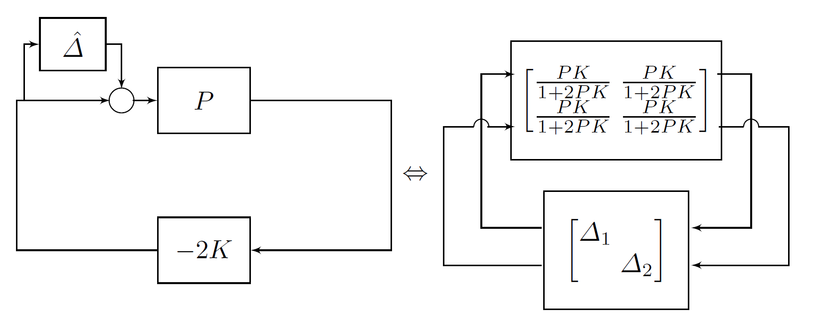
Figure 4: Reshaped loop of two-agent system with correlated uncertainties.

Theorem 3.2.

There exists a consensus protocol (12) achieving mean square consensus for the two-agent system in (11) if and only if

$$\frac{1}{4}(\sigma_{1}^{2}+2\sigma_{12}+\sigma_{2}^{2})(p_{1}^{2}-1)<1.$$ (14)

Following similar steps in the proof of Theorem 3.1, it is not difficult to verify the condition (14). The details are omitted here for conciseness. As a remark, we point out that when the agents contain no eigenvalues outside the unit circle, i.e., $p_{1}=\pm 1$, one can show that the condition (14) always holds. The implication then is that no matter how large the variance of the uncertainty is, we can always find a feedback $K$ to guarantee the robust mean square consensus.

4 Illustrative Example

We use two examples to examine the preceding results in Theorem 3.1 and 3.2.

Example 1 Consider first the first-order system (5) with an unstable pole $p_{1}=\sqrt{2}$. It is instructive to examine the three-dimensional (3-D) manifold of $(\sigma_{1}^{2},\sigma_{2}^{2},\sigma_{12})$, to see the corresponding mean-square stabilizable region (also mean-square unstabilizable region) with respect to the stochastic uncertainties $\Delta_{1}$ and $\Delta_{2}$. Fig. 5 $(a)$ gives approximately the mean-square stabilizable region in terms of $(\sigma_{1}^{2},\sigma_{2}^{2},\sigma_{12})$, which constitutes an unbounded convex hull. We next examine the the first-order nonminimum phase system (6) with a nonminimum phase zero $s_{1}=2\sqrt{2}$. Fig. 5 $(b)$ characterizes the mean-square stabilizable region accordingly. Apparently, the presence of nonminimum phase zero drastically reduces the feasible region for the mean-square stabilization, following one’s long-held intuition.

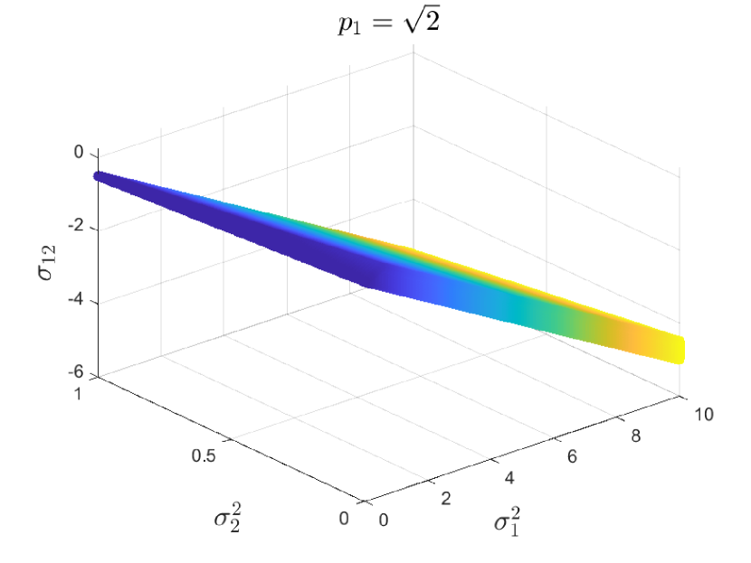
$(a)$

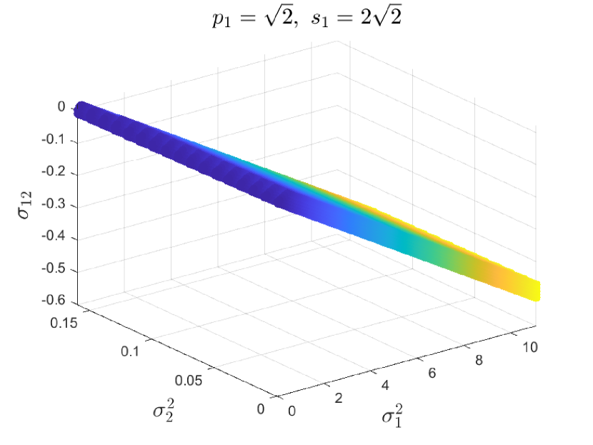
$(b)$

Figure 5: Mean-square stabilizable region for $(\sigma_{1}^{2},\sigma_{2}^{2},\sigma_{12})$.

We may also fix the triple $(\sigma_{1}^{2},\sigma_{2}^{2},\sigma_{12})=(0.2,0.1,0.05)$ and verify the mean-square stabilizable region for all $p_{1}\geq 1$. Fig. 6 $(a)$ shows that when $p_{1}\in[1,~{}2.3453)$, the system (5) is mean-square stabilizable. Next, with fixing $p_{1}=\sqrt{2}$, we can conclude from Fig. 6 $(b)$ that the nonminimum phase system (6) is mean-square stabilizable if $s_{1}\geq 4.7021$. This observation is consistent with a well-accepted agreement, that is a zero-pole closeness is detrimental to the robust stabilization.

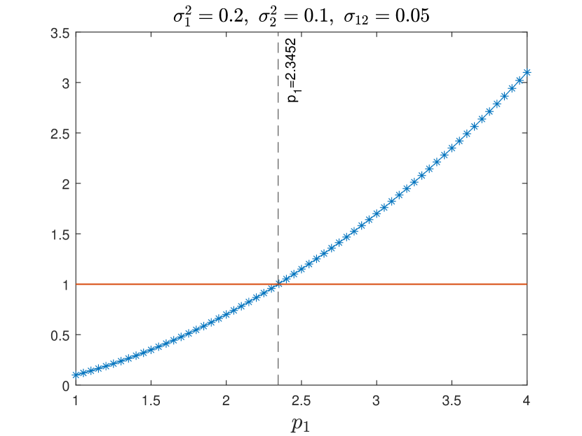
$(a)$

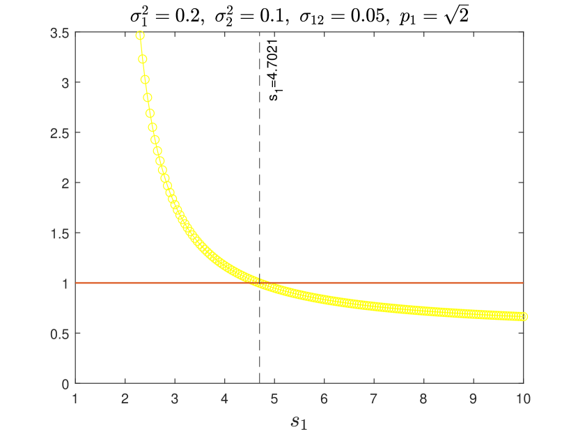
$(b)$

Figure 6: Mean-square stabilizable region for $p_{1}$ and $s_{1}$.

Example 2 Following from (14), the mean-square consensusability of the two-agent system (11) is codetermined by the unstable pole $p_{1}$ and the variance $\sigma_{1}^{2}+2\sigma_{12}+\sigma_{2}^{2}$ together and the feasible region has been filled in Fig. 7. The inversely proportional relationship between $p_{1}$ and $\sigma_{1}^{2}+2\sigma_{12}+\sigma_{2}^{2}$ hence is clearly.

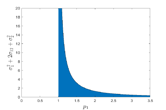
Figure 7: The region of mean-square consensusability for $p_{1}$ and $\sigma_{1}^{2}+2\sigma_{12}+\sigma_{2}^{2}$

5 Conclusion

In this paper we have studied mean-square stabilizability and consensusability problems for networked control systems over uncertain communication channels. We modelled each communication channel as an ideal transmission system subject to a multiplicative stochastic perturbation. All perturbations from different channels are allowed to be correlated in spatial. We first presented fundamental conditions to ensure the mean-square stability of the open-loop stable system under such uncertainties. Next, given two kind of unstable low-order systems, we provided the stabilizability or consensusability conditions linking together such system dynamics and uncertainty variances, under which the robust stable or consensus can be ensured. Notably, all obtained main conditions are necessary and sufficient in the paper.

References

• [1] D. Hinrichsen and A. J. Pritchard, “Stability radii of systems with stochastic uncertainty and their optimization by output feedback,” SIAM journal on control and optimization, vol. 34, no. 6, pp. 1972–1998, 1996.
• [2] R. W. Brockett and D. Liberzon, “Quantized feedback stabilization of linear systems,” IEEE transactions on Automatic Control, vol. 45, no. 7, pp. 1279–1289, 2000.
• [3] N. Elia, “Remote stabilization over fading channels,” Systems & Control Letters, vol. 54, no. 3, pp. 237–249, 2005.
• [4] J. Lu and R. E. Skelton, “Mean-square small gain theorem for stochastic control: discrete-time case,” IEEE Transactions on Automatic Control, vol. 47, no. 3, pp. 490–494, 2002.
• [5] J. H. Braslavsky, R. H. Middleton, and J. S. Freudenberg, “Feedback stabilization over signal-to-noise ratio constrained channels,” IEEE Transactions on Automatic Control, vol. 52, no. 8, pp. 1391–1403, 2007.
• [6] L. Schenato, B. Sinopoli, M. Franceschetti, K. Poolla, and S. S. Sastry, “Foundations of control and estimation over lossy networks,” Proceedings of the IEEE, vol. 95, no. 1, pp. 163–187, 2007.
• [7] B. Bamieh, “Structured stochastic uncertainty,” in Communication, Control, and Computing (Allerton), 2012 50th Annual Allerton Conference on.   IEEE, 2012, pp. 1498–1503.
• [8] T. Qi, J. Chen, W. Su, and M. Fu, “Control under stochastic multiplicative uncertainties: Part i, fundamental conditions of stabilizability,” IEEE Transactions on Automatic Control, vol. 62, no. 3, pp. 1269–1284, 2017.
• [9] W. Su, J. Chen, M. Fu, and T. Qi, “Control under stochastic multiplicative uncertainties: Part ii, optimal design for performance,” IEEE Transactions on Automatic Control, vol. 62, no. 3, pp. 1285–1300, 2017.
• [10] J. Chen, S. He, and J. Chen, “Mean-square stability conditions for linear systems with random delays,” in 2018 13th World Congress on Intelligent Control and Automation (WCICA).   IEEE, 2018, pp. 614–619.
• [11] K. You and L. Xie, “Minimum data rate for mean square stabilization of discrete lti systems over lossy channels,” IEEE Transactions on Automatic Control, vol. 55, no. 10, pp. 2373–2378, 2010.
• [12] K. Zhou, J. C. Doyle, K. Glover et al., Robust and Optimal Control.   Prentice hall New Jersey, 1996, vol. 40.
• [13] J. L. Willems and J. C. Willems, “Feedback stabilizability for stochastic systems with state and control dependent noise,” Automatica, vol. 12, no. 3, pp. 277–283, 1976.
• [14] S. Boyd, L. El Ghaoui, E. Feron, and V. Balakrishnan, Linear Matrix Inequalities in System and Control Theory.   SIAM, 1994.
• [15] E. B. Davies, Linear Operators and Their Spectra.   Cambridge University Press, 2007, vol. 106.
• [16] B.-S. Tam and S.-F. Wu, “On the Collatz-Wielandt sets associated with a cone-preserving map,” Linear Algebra and its Applications, vol. 125, pp. 77–95, 1989.
• [17] W. Chen and L. Qiu, “Linear quadratic optimal control of continuous-time LTI systems with random input gains,” IEEE Transactions on Automatic Control, vol. 61, no. 7, pp. 2008–2013, 2015.
• [18] K. Ogata, Discrete-Time Control Systems.   Prentics-Hall, Inc, 1994.