Segmenting Time Series via Self-Normalization

Abstract

We propose a novel and unified framework for change-point estimation in multivariate time series. The proposed method is fully nonparametric, robust to temporal dependence and avoids the demanding consistent estimation of long-run variance. One salient and distinct feature of the proposed method is its versatility, where it allows change-point detection for a broad class of parameters (such as mean, variance, correlation and quantile) in a unified fashion. At the core of our method, we couple the self-normalization (SN) based tests with a novel nested local-window segmentation algorithm, which seems new in the growing literature of change-point analysis. Due to the presence of an inconsistent long-run variance estimator in the SN test, non-standard theoretical arguments are further developed to derive the consistency and convergence rate of the proposed SN-based change-point detection method. Extensive numerical experiments and relevant real data analysis are conducted to illustrate the effectiveness and broad applicability of our proposed method in comparison with state-of-the-art approaches in the literature.

Keywords: Binary segmentation; Change-point detection; Scanning; Studentization; Long-run variance; Temporal dependence

1 Introduction

Change-point detection has been identified as one of the major challenges for modern data applications (National Research Council,, 2013). There is a vast literature on change-point estimation and testing in statistics, in part due to its broad applications in bioinformatics, climate science, economics, finance, genetics, medical science, and signal processing among many other areas. See Csörgő and Horváth, (1997), Brodsky and Darkhovsky, (2013) and Tartakovsky et al., (2014) for book-length treatments of the subject. We also refer to Aue and Horváth, (2013), Casini and Perron, (2019) and Truong et al., (2020) for excellent reviews.

In this paper, we study the problem of time series segmentation, also known as (offline) change-point estimation, where the task is to partition a sequence of potentially non-homogeneous ordered observations into piecewise homogeneous segments. Many change-point problems arise within a time series context (e.g. climate, epidemiology, economics and financial data), where there is a natural temporal ordering in the observations. Although temporal dependence is the norm rather than the exception for time series, most literature in change-point analysis assume and require independence of observations $\{Y_{t}\}_{t=1}^{n}$ over time for methodological and theoretical validity; see for example Olshen et al., (2004), Killick et al., (2012), Matteson and James, (2014), Fryzlewicz, (2014), and Baranowski et al., (2019) among others. One stream of literature addresses temporal dependence via the assumption of parametric models, see Davis et al., (2006) and Yau and Zhao, (2016) for change-point detection in AR process and Fryzlewicz and Subba-Rao, (2014) in ARCH process. However, parametric approaches generally require stronger conditions and potential violation of parametric assumptions can inevitably cast doubts on the estimation result.

Existing nonparametric approaches for change-point estimation in temporally dependent observations primarily focus on first or second-order moments, see Bai and Perron, (1998), Eichinger and Kirch, (2018) for change-point estimation in mean, Aue et al., (2009), Preuss et al., (2015) in (auto)-covariance, and Cho and Fryzlewicz, (2012), Casini and Perron, 2021a in spectral density function (thus second-order properties). However, for many applications, the key interest can go beyond mean or covariance. For example, detecting potential changes in extreme quantiles is critical for monitoring systemic risk (i.e. Value-at-Risk) in finance and for studying evolving behavior of severe weather systems such as hurricanes in climate science. Moreover, existing nonparametric methods are mostly designed for detecting only one specific type of change (e.g. mean or variance) and cannot be universally used for examining changes in different aspects of the data, which may limit its applications and cause inconvenience of implementation for practitioners. Additionally, existing nonparametric procedures typically involve certain tuning or smoothing parameters, such as the bandwidth parameter involved in the consistent estimation of the long-run variance, and how to choose these tuning parameters is important yet highly challenging in practice.

To fill in the gap in the literature, we propose a new multiple change-point estimation framework that is fully nonparametric, robust to temporal dependence, enjoys effortless tuning, and works universally for various parameters of interest for a multivariate time series $\{Y_{t}\}_{t=1}^{n}$ where $Y_{t}\in\mathbb{R}^{p}$ with a fixed dimension $p\geq 1$. Specifically, denote $F_{t}$ as the cumulative distribution function (CDF) of $Y_{t}$, the proposed procedure allows change-point detection for any $\theta$ such that $\theta=\theta(F_{t})$, where $\theta(\cdot)$ is a functional that takes value in $\mathbb{R}^{d}$ with $d\geq 1.$ This is a broad framework that covers important quantities such as mean, variance, quantile, (auto)-correlation and (auto)-covariance among others, see Künsch, (1989) and Shao, (2010).

As in the standard change-point literature, we assume the change happens in a piecewise constant fashion. Specifically, we assume $\{Y_{t}\}_{t=1}^{n}$ is a piecewise stationary time series and there exist $m_{o}\geq 0$ unknown number of change-points $0<k_{1}<\cdots<k_{m_{o}}<n$ that partition $\{Y_{t}\}_{t=1}^{n}$ into $m_{o}+1$ stationary segments. Define $k_{0}=0$ and $k_{m_{o}+1}=n$, the $i$th segment contains stationary observations $\{Y_{t}\}_{t=k_{i-1}+1}^{k_{i}}$ that share common behavior characterized by $\theta_{i}$ (e.g. mean, variance, correlation, quantile), where we require $\theta_{i}\not=\theta_{i+1}$ for $i=1,\cdots,m_{o}$ due to the structural break. Our primary interest is to recover the unknown number and locations of the change-points.

To achieve broad applicability and robustness against temporal dependence, our proposed multiple change-point estimation method is built upon self-normalization (SN, hereafter), a nascent inference technique for time series (Shao,, 2010, 2015). We note that since its first proposal in Shao, (2010), SN has been extended to retrospective change-point testing by Shao and Zhang, (2010), Hoga, (2018), Betken and Wendler, (2018), Zhang and Lavitas, (2018), and Dette et al., (2020), and to sequential change-point monitoring by Dette and Gösmann, (2020) and Chan et al., (2021). However, the primary focus of these papers is to construct SN-based change-point testing procedures (either retrospective or sequential) but not change-point estimation. Compared to change-point testing, change-point estimation is a much more challenging task both methodologically and theoretically: it further requires the estimation of the unknown number and locations of change-points, which involves substantially different techniques and analysis.

Indeed, the use of SN for time series segmentation (i.e. multiple change-point estimation) seems largely unexplored, with the exception of Jiang et al., (2020, 2022) for piecewise linear and quantile trend models designed for COVID-19 time series. One notable reason for the scarcity of SN-based time series segmentation algorithms is that, unlike the classical CUSUM-based change-point test, the SN-based change-point testing cannot be easily extended to multiple change-point estimation by combining with the standard binary segmentation algorithm (Vostrikova,, 1981). Such a combination simply fails due to the potential inflation of the self-normalizer under the presence of multiple change-points. We discuss this point in more details later in Section 3 and provide further illustration via both theory and numerical experiments in Section S.1 of the supplementary material.

To bypass this difficulty, we propose a novel nested local-window segmentation algorithm, which is then combined with an SN test to achieve multiple change-point estimation. We name the procedure SNCP. Through a series of carefully designed nested local-windows, the proposed procedure can isolate each true change-point adaptively and thus achieves respectable detection power and estimation accuracy. The statistical and computational efficiency of the nested local-window segmentation algorithm is further illustrated via extensive numerical comparison with popular segmentation algorithms such as SaRa in Niu and Zhang, (2012), WBS in Fryzlewicz, (2014) and SBS in Kovacs et al., (2020).

In addition to methodological advances, new theoretical arguments based on the partial influence functions (Pires and Branco,, 2002) are further developed to establish the consistency and convergence rate of the proposed change-point estimation procedure, which seems to be the first in the SN literature. The proof is non-standard and built on a subtle analysis of the behavior of SN-based test statistic around change-points. It differs from existing techniques in the change-point literature due to the presence of the self-normalizer (an inconsistent long-run variance estimator) and is of independent interest.

To our best knowledge, the proposed method (SNCP) is the first to address multiple change point estimation for a general parameter in the time series setting. One salient and distinct feature of SNCP is its versatility: it allows the user to examine potential change in virtually any parameter of interest in an effortless fashion. This is valuable as in practice, the ground truth is unknown and it is important to examine the behavior change of the data via different angles. In addition, due to its versatility and robustness to temporal dependence, SNCP can serve as a numerically credible and theoretically valid benchmark for almost all algorithms designed for multiple change-point estimation in a fixed-dimensional time series, which is of interest to both practical applications and academic research.

The rest of the paper is organized as follows. We first provide background of SN and introduce the SN-based detection method for single change-point estimation in Section 2. Building upon a novel nested local-window segmentation algorithm, Section 3 proposes a unified SN-based framework (SNCP) for multiple change-point estimation and further studies its theoretical properties. Extensive numerical experiments are conducted in Section 4 to demonstrate the promising performance of SNCP when compared with state-of-the-art methods for change-point estimation in mean, variance, quantile of univariate time series, and correlation and covariance matrix of multivariate time series. Section 5 concludes. Technical proofs and additional simulation and real data application results can be found in the supplement.

Some notations used throughout the paper are defined as follows. Let $D[0,1]$ denote the space of functions on $[0,1]$ which are right continuous with left limits, endowed with the Skorokhod topology (Billingsley,, 1968). We use $\Rightarrow$ to denote weak convergence in $D[0,1]$ or more generally in $\mathbb{R}^{m}$-valued function space $D^{m}[0,1]$, where $m\in\mathbb{N}$. We use $\overset{\mathcal{D}}{\longrightarrow}$ to denote convergence in distribution. We use $\|\cdot\|_{2}$ to denote the $l_{2}$ norm of a vector and use $\|\cdot\|$ to denote the spectral norm of a matrix.

2 Single Change-point Estimation

In this section, we provide some background on the SN test and propose an SN test based method for single change-point estimation, which serves as a building block for the proposed multiple change-point estimation procedure in Section 3. Model assumptions and consistency results are discussed in details to provide intuition and foundation for more involved results in Section 3. For ease of presentation, in the following we assume $d=1$, in other words, the parameter of interest $\theta$ is univariate, and postpone the results for the multivariate case of $d>1$ to Section 3.3.

2.1 An SN-based estimation procedure

We start with single change-point estimation in a general parameter $\theta=\theta(F_{t})$ for a univariate time series $\{Y_{t}\}_{t=1}^{n}$, where $F_{t}$ denotes the CDF of $Y_{t}$ and $\theta(\cdot)$ is a general functional. Under the no change-point scenario, $\{Y_{t}\}_{t=1}^{n}$ is a stationary time series. Under the single change-point alternative, we follow the framework of Dette and Gösmann, (2020) and assume $\{Y_{t}\}_{t=1}^{n}$ is generated by

$$Y_{t}=\begin{cases}Y_{t}^{(1)},&1\leq t\leq k_{1}\\ Y_{t}^{(2)},&k_{1}+1\leq t\leq n,\\ \end{cases}$$ (1)

where $\{Y_{t}^{(i)}\}_{t\in\mathbb{Z}}$ is a stationary time series with $Y_{t}^{(i)}\sim F^{(i)}$ for $i=1,2$. Thus we have $F_{t}=F^{(1)}\mathbf{1}(t\leq k_{1})+F^{(2)}\mathbf{1}(t>k_{1})$. Denote $\theta_{1}=\theta(F^{(1)})$ and $\theta_{2}=\theta(F^{(2)})$, we have $\delta=\theta_{2}-\theta_{1}\neq 0$ and the change-point $k_{1}=\lfloor n\tau_{1}\rfloor$ with $\tau_{1}\in(0,1)$. Note that the dependence between $\{Y_{t}^{(1)}\}$ and $\{Y_{t}^{(2)}\}$ is deliberately left unspecified, as the validity of the proposed method does not rely on the specification of the dependence (see Assumption 2.1(i) for more details).

To detect the existence and further estimate the location of the (potential) single change-point $k_{1}=\lfloor n\tau_{1}\rfloor$, we propose an SN-based testing approach. Specifically, we define

$$SN_{n}=\max_{k=1,\cdots,n-1}T_{n}(k),\quad T_{n}(k)=D_{n}(k)^{2}/V_{n}(k),$$ (2)

where

$$\begin{split}D_{n}(k)=&\frac{k(n-k)}{n^{3/2}}(\widehat{\theta}_{1,k}-\widehat{\theta}_{k+1,n}),\\ V_{n}(k)=&\sum_{i=1}^{k}\frac{i^{2}(k-i)^{2}}{n^{2}k^{2}}(\widehat{\theta}_{1,i}-\widehat{\theta}_{i+1,k})^{2}+\sum_{i=k+1}^{n}\frac{(n-i+1)^{2}(i-k-1)^{2}}{n^{2}(n-k)^{2}}(\widehat{\theta}_{i,n}-\widehat{\theta}_{k+1,i-1})^{2},\end{split}$$ (3)

and for any $1\leq a<b\leq n$, $\widehat{\theta}_{a,b}=\theta(\widehat{F}_{a,b})$ where $\widehat{F}_{a,b}$ is the empirical distribution of $\{Y_{t}\}_{t=a}^{b}$. In other words, $\widehat{\theta}_{a,b}$ denotes the nonparametric estimator of $\theta$ based on the subsample $\{Y_{t}\}_{t=a}^{b}$.

When $\theta(\cdot)$ is the mean functional, i.e., $\theta(F_{t})=\int xF_{t}(dx)$, the newly defined contrast-based test $SN_{n}$ in (2) reduces to the CUSUM-based SN test statistic in Shao and Zhang, (2010) (cf. equation (4) therein). However, for a nonlinear functional $\theta(\cdot)$, such as variance, correlation and quantile, $SN_{n}$ is not equivalent to the CUSUM-based counterpart and is preferred due to its contrast nature. We refer to Zhang and Lavitas, (2018) for more discussion.

Built upon the test statistic defined in (2), the SN-based change-point detection procedure proceeds as follows. For a pre-specified threshold $K_{n}$, we declare no change-point if $SN_{n}\leq K_{n}$. Given that $SN_{n}$ exceeds the threshold, we estimate the single change-point location via

$$\widehat{k}=\arg\max_{k=1,\cdots,n-1}T_{n}(k).$$

This SN-based procedure provides a general and unified change-point estimation framework, as it can be implemented for any functional $\theta(\cdot)$ with a nonparametric estimator based on the empirical distribution.

2.2 Assumptions and theoretical results

To establish the consistency of the SN-based estimation procedure under the general functional setting (1), the key is to track the asymptotic behavior of $\widehat{\theta}_{a,b}$ for $1\leq a<b\leq n$. To achieve this, we operate under the framework of approximately linear functional, which covers important quantities such as mean, variance, covariance, correlation and quantile (Künsch,, 1989; Shao,, 2010).

Specifically, we assume the subsample estimator $\widehat{\theta}_{a,b}$ admits the following expansion on the stationary time series $\{Y_{t}^{(i)}\},i=1,2,$ where

$$\begin{split}\widehat{\theta}_{a,b}=&\theta_{1}+\frac{1}{b-a+1}\sum_{t=a}^{b}\xi_{1}(Y_{t}^{(1)})+r^{(1)}_{a,b},\quad\text{for}~{}b\leq k_{1},\\ \widehat{\theta}_{a,b}=&\theta_{2}+\frac{1}{b-a+1}\sum_{t=a}^{b}\xi_{2}(Y_{t}^{(2)})+r^{(2)}_{a,b},\quad\text{for}~{}a>k_{1}.\end{split}$$ (4)

In other words, $\widehat{\theta}_{a,b}$ is approximately linear when the subsample $\{Y_{t}\}_{t=a}^{b}$ is stationary. Note that $\xi_{1}(Y_{t}^{(1)})$ and $\xi_{2}(Y_{t}^{(2)})$ are indeed the influence functions of the functional $\theta(\cdot)$ (Hampel et al.,, 1986), which is the leading term for asymptotic behavior of $\widehat{\theta}_{a,b}$, and $r^{(1)}_{a,b},r^{(2)}_{a,b}$ are the remainder terms.

To further regulate the behavior of $\widehat{\theta}_{a,b}$ when the subsample $\{Y_{t}\}_{t=a}^{b}$ is a mixture of two stationary segments, we utilize the concept of partial influence functions originated from the robust statistics literature (Pires and Branco,, 2002). Specifically, for $a\leq k_{1}<b$, we assume

$$\widehat{\theta}_{a,b}= \theta(\omega_{a,b})+\frac{1}{b-a+1}\left[\sum_{t=a}^{k_{1}}\xi_{1}(Y_{t}^{(1)},\omega_{a,b})+\sum_{t=k_{1}+1}^{b}\xi_{2}(Y_{t}^{(2)},\omega_{a,b})\right]+r_{a,b}(\omega_{a,b}),$$ (5)

where $\omega_{a,b}=\left(\omega_{a,b}^{(1)},\omega_{a,b}^{(2)}\right)^{\top}=\left(\frac{k_{1}-a+1}{b-a+1},\frac{b-k_{1}}{b-a+1}\right)^{\top}$ denotes the proportion of each stationary segment in $\{Y_{t}\}_{t=a}^{b}$, $\theta(\omega_{a,b})$ denotes $\theta(\cdot)$ evaluated at the mixture distribution $F^{\omega_{a,b}}=\omega_{a,b}^{(1)}F^{(1)}+\omega_{a,b}^{(2)}F^{(2)}$ and $r_{a,b}(\omega_{a,b})$ is the remainder term. The terms $\xi_{1}(Y_{t}^{(1)},\omega_{a,b})$ and $\xi_{2}(Y_{t}^{(2)},\omega_{a,b})$ are related to the partial influence functions of the functional $\theta(\cdot)$ evaluated at the mixture distribution $F^{\omega_{a,b}}$. See detailed discussion later.

Note that the expansion (5) generalizes (4) under the single change-point scenario. Specifically, define $\omega_{a,b}=(1,0)^{\top}$ and $(0,1)^{\top}$ for $b\leq k_{1}$ and $a>k_{1}$ respectively, (4) can be viewed as a special case of (5) where the mixture distribution is pure such that $\xi_{1}(Y_{t}^{(1)})=\xi_{1}(Y_{t}^{(1)},(1,0)^{\top})$, $r_{a,b}^{(1)}=r_{a,b}((1,0)^{\top})$ and $\xi_{2}(Y_{t}^{(2)})=\xi_{2}(Y_{t}^{(2)},(0,1)^{\top})$, $r_{a,b}^{(2)}=r_{a,b}((0,1)^{\top})$ respectively.

We now work out the explicit formulation of the expansion (5) under the framework of partial influence function (Pires and Branco,, 2002). Denote the mixture weight $\omega=(\omega^{(1)},\omega^{(2)})^{\top}$ such that $\omega^{(i)}\in[0,1]$, $i=1,2$ and $\omega^{(1)}+\omega^{(2)}=1$. Denote $\theta(\omega,F^{(1)},F^{(2)}):=\theta(\omega^{(1)}F^{(1)}+\omega^{(2)}F^{(2)})$ as the functional $\theta(\cdot)$ evaluated at the mixture $F^{\omega}:=\omega^{(1)}F^{(1)}+\omega^{(2)}F^{(2)}$. Definition 2.1 defines the partial influence function as in Pires and Branco, (2002).

Definition 2.1.

The partial influence functions of the functional $\theta(F^{\omega})=\theta(\omega,F^{(1)},F^{(2)})$ with relation to $F^{(1)}$ and $F^{(2)}$, respectively, are given by

$$IF_{1}\left(y,\theta(\omega,F^{(1)},F^{(2)})\right)= \lim\limits_{\epsilon\to 0}\epsilon^{-1}\Big{[}\theta\left(\omega,(1-\epsilon)F^{(1)}+\epsilon\delta_{y},F^{(2)}\right)-\theta(\omega,F^{(1)},F^{(2)})\Big{]},$$

$$IF_{2}\left(y,\theta(\omega,F^{(1)},F^{(2)})\right)= \lim\limits_{\epsilon\to 0}\epsilon^{-1}\Big{[}\theta\left(\omega,F^{(1)},(1-\epsilon)F^{(2)}+\epsilon\delta_{y}\right)-\theta(\omega,F^{(1)},F^{(2)})\Big{]},$$

provided the limits exist, where $\delta_{y}$ is the Dirac mass at $y$.

To understand the partial influence functions, define $\zeta=\omega^{(1)}\epsilon$, by Definition 2.1, we have

$$IF_{1}\left(y,\theta(\omega,F^{(1)},F^{(2)})\right)= \omega^{(1)}\lim\limits_{\zeta\to 0}\zeta^{-1}\Big{[}\theta\left((\delta_{y}-F^{(1)})\zeta+F^{\omega}\right)-\theta\left(F^{\omega}\right)\Big{]}=\omega^{(1)}\xi_{1}(y,\omega),$$

where $\xi_{1}(y,\omega)$ is the Gâteaux derivative of $\theta\big{(}F^{\omega}\big{)}$ in the direction $\delta_{y}-F^{(1)}$. Similarly, $IF_{2}\left(y,\theta(\omega,F^{(1)},F^{(2)})\right)=\omega^{(2)}\xi_{2}(y,\omega)$, where $\xi_{2}(y,\omega)$ is the Gâteaux derivative of $\theta\big{(}F^{\omega}\big{)}$ in the direction $\delta_{y}-F^{(2)}$.

To establish the expansion (5), note that $\widehat{\theta}_{a,b}=\theta(\widehat{F}_{a,b})$, where $\widehat{F}_{a,b}$ denotes the empirical CDF based on the subsample $\{Y_{t}\}_{t=a}^{b}$. The key observation is that $\widehat{F}_{a,b}=\omega^{(1)}_{a,b}\widehat{F}_{a,k_{1}}+\omega^{(2)}_{a,b}\widehat{F}_{k_{1}+1,b}$ with $\omega_{a,b}=\left(\frac{k_{1}-a+1}{b-a+1},\frac{b-k_{1}}{b-a+1}\right)^{\top}$. In other words, $\widehat{F}_{a,b}$ can be viewed as a mixture of two empirical CDFs $\widehat{F}_{a,k_{1}}$ and $\widehat{F}_{k_{1}+1,b}$ based on stationary segments with CDF $F^{(1)}$ and $F^{(2)}$ respectively. Thus, by the results in Pires and Branco, (2002), we have

$$\theta(\widehat{F}_{a,b})= \theta\left(F^{\omega_{a,b}}\right)+\frac{1}{k_{1}-a+1}\sum_{t=a}^{k_{1}}IF_{1}\left(Y_{t}^{(1)},\theta(\omega_{a,b},F^{(1)},F^{(2)})\right)$$

$$+\frac{1}{b-k_{1}}\sum_{t=k_{1}+1}^{b}IF_{2}\left(Y_{t}^{(2)},\theta(\omega_{a,b},F^{(1)},F^{(2)})\right)+R(\widehat{F}_{a,b}-F^{\omega_{a,b}}),$$

where $R(\widehat{F}_{a,b}-F^{\omega_{a,b}})$ denotes the remainder term. The expansion (5) follows immediately by substituting the partial influence functions with the Gâteaux derivatives $\xi_{1}(y,\omega_{a,b})$ and $\xi_{2}(y,\omega_{a,b})$.

We proceed by imposing the following Assumptions 2.1-2.3 on the approximately linear functional $\theta(\cdot)$, which are further verified in Section S.4 of the supplement for the smooth function model (including mean, variance, (auto)-covariance, (auto)-correlation) and in Section S.5 of the supplement for quantile. We refer to Remark 1 in Section 3.2 for more detailed discussion on the verification of assumptions.

Assumption 2.1.

$(\mathrm{i})$ For some $\sigma_{1}>0$ and $\sigma_{2}>0$, we have

$$\frac{1}{\sqrt{n}}\sum_{t=1}^{[nr]}\Big{(}\xi_{1}(Y_{t}^{(1)}),\xi_{2}(Y_{t}^{(2)})\Big{)}\Rightarrow(\sigma_{1}B^{(1)}(r),\sigma_{2}B^{(2)}(r)),$$

where $B^{(1)}(\cdot)$ and $B^{(2)}(\cdot)$ are standard Brownian motions.

$(\mathrm{ii})$ $\sup_{k<k_{1}}\left|\sum_{t=k+1}^{k_{1}}\xi_{1}\left(Y_{t}^{(1)},\omega_{k+1,n}\right)+\sum_{t=k_{1}+1}^{n}\xi_{2}\left(Y_{t}^{(2)},\omega_{k+1,n}\right)\right|=O_{p}(n^{1/2}),$
     $\sup_{k>k_{1}}\left|\sum_{t=1}^{k_{1}}\xi_{1}(Y_{t}^{(1)},\omega_{1,k})+\sum_{t=k_{1}+1}^{k}\xi_{2}(Y_{t}^{(2)},\omega_{1,k})\right|=O_{p}(n^{1/2}).$

Assumption 2.2.

$\sup_{1\leq k\leq n}k|r_{1,k}(\omega_{1,k})|+\sup_{1\leq k\leq n}(n-k+1)|r_{k,n}(\omega_{k,n})|=o_{p}(n^{1/2}).$

Assumption 2.1 regulates the behavior of the (partial) influence function $\xi_{1}(\cdot)$ and $\xi_{2}(\cdot)$. Specifically, Assumption 2.1(i) requires the invariance principle to hold for each stationary segment. Note that the dependence of the two Brownian motions $B^{(1)}(\cdot)$ and $B^{(2)}(\cdot)$ are left unspecified as we do not require a specific dependence structure on $\{Y_{t}^{(1)}\}$ and $\{Y_{t}^{(2)}\}$. Assumption 2.1(ii) are tailored to regulate $\widehat{\theta}_{a,b}$ estimated on a mixture of two stationary segments. Assumption 2.2 requires that the remainder term is asymptotically negligible and is a commonly used assumption in the SN literature (Shao,, 2010, 2015).

Assumption 2.3.

Denote $\theta(\omega)=\theta(\omega^{(1)}F^{(1)}+\omega^{(2)}F^{(2)})$, where $\omega=(\omega^{(1)},\omega^{(2)})^{\top}$ is the mixture weight with $\omega^{(i)}\in[0,1],i=1,2$ and $\omega^{(1)}+\omega^{(2)}=1$. There exist some constants $0<C_{1}<C_{2}<\infty$ such that for any mixture weight $\omega$, we have

$$C_{1}\omega^{(2)}|\theta_{1}-\theta_{2}|\leq|\theta_{1}-\theta(\omega)|\leq C_{2}\omega^{(2)}|\theta_{1}-\theta_{2}|\text{ and }C_{1}\omega^{(1)}|\theta_{1}-\theta_{2}|\leq|\theta_{2}-\theta(\omega)|\leq C_{2}\omega^{(1)}|\theta_{1}-\theta_{2}|.$$

Assumption 2.3 regulates the smoothness of $\theta(\omega)$. Intuitively, it means that the functional $\theta(\cdot)$ can distinguish the mixture distribution $w^{(1)}F^{(1)}+w^{(2)}F^{(2)}$ from $F^{(1)}$ and $F^{(2)}$. For mean functional, we have $\theta(\omega)=\omega^{(1)}\theta_{1}+\omega^{(2)}\theta_{2}$, thus we can set $C_{1}=C_{2}=1$ as $\theta(\omega)$ is linear in $\omega$.

Assumption 2.4.

$n\delta^{2}\to\infty$ as $n\to\infty$, and $K_{n}$ satisfies $K_{n}=(n\delta^{2})^{\kappa}$ for some $\kappa\in(\frac{1}{2},1)$.

Assumption 2.4 quantifies the asymptotic order of the change size $\delta$ and the threshold $K_{n}$. Under Assumptions 2.1-2.4, Theorem 2.1 gives the consistency results of the SN-based change-point estimation method for approximately linear functionals.

Theorem 2.1.

$(\mathrm{i})$ Under the no change-point scenario, suppose Assumptions 2.1(i) and 2.2 hold, we have $SN_{n}\overset{\mathcal{D}}{\longrightarrow}G=\sup_{r\in[0,1]}\{B(r)-rB(1)\}^{2}/V(r),$ where $B(\cdot)$ denotes a standard Brownian motion and $V(r)=\int_{0}^{r}[B(s)-(s/r)B(r)]^{2}ds+\int_{r}^{1}[B(1)-B(s)-(1-s)/(1-r)\{B(1)-B(r)\}]^{2}ds$.
$(\mathrm{ii})$ Under the one change-point scenario, suppose Assumptions 2.1-2.4 hold, we have

$$\lim\limits_{n\to\infty}P(T_{n}(\widehat{k})>K_{n}\quad\text{and}\quad|\widehat{k}-k_{1}|\leq\iota_{n})=1,$$

for any sequence $\iota_{n}$ such that $\iota_{n}/n\to 0$ and $\iota_{n}^{-2}\delta^{-2}n\to 0$ as $n\to\infty$.

Theorem 2.1(i) indicates that the asymptotic distribution of $SN_{n}$ for a general functional $\theta(\cdot)$ coincides with the asymptotic distribution of the CUSUM-based SN test for mean (see Theorem 3.1 in Shao and Zhang, (2010)). This implies that the same threshold $K_{n}$ can be used to control false positives (i.e. Type-I error) for change-point detection in various parameters and thus greatly simplifies the implementation of the proposed method. In practice, we recommend to set $K_{n}$ as the 90% or 95% quantile of $G$, which can be obtained via simulation as $G$ is pivotal. See Shao and Zhang, (2010) for tabulated critical values of $G$.

Theorem 2.1(ii) gives the convergence rate of the estimated change-point $\widehat{k}$, providing a unified theoretical justification of the SN-based method for a broad class of functionals. Due to the presence of the self-normalizer $V_{n}(k)$, which is complex and further varies by $k$, nonstandard technical arguments different from existing techniques in the change-point literature are developed to establish the consistency result. It involves a simultaneous analysis of the contrast statistic $D_{n}(k)$ and the self-normalizer $V_{n}(k)$. In general, the localization error rate of SNCP is not optimal (at least for change in mean). However, a simple local refinement procedure can be performed to help achieve the optimal rate. We refer to the discussion following 3.1 in Section 3.2 for more details on this matter.

The traditional CUSUM based estimation procedure in the change-point literature typically admits the form $\max_{k=1,\cdots,n-1}|D_{n}(k)|/\widehat{\sigma}_{n}$, where theoretical results are derived under the assumption that $\widehat{\sigma}_{n}$ is a consistent estimator of the long-run variance (LRV), leading to less involved technical analysis than the proposed SN-based estimation. However, in practice, the construction of a consistent $\widehat{\sigma}_{n}$ involves a bandwidth tuning parameter that is difficult to select, especially under the presence of change-points. For example, in the mean case, using a data-driven bandwidth with the estimation-optimal bandwidth formula in Andrews, (1991) could lead to non-monotonic power under the change-point alternative and large size distortion under the null, see Crainiceanu and Vogelsang, (2007) and Shao and Zhang, (2010). Casini et al., (2021) and Casini and Perron, 2021b further provide a comprehensive theoretical analysis of such phenomenon based on Edgeworth expansion. Additionally, different construction of $\widehat{\sigma}_{n}$ is required for different functional $\theta(\cdot)$, which can be highly involved and non-trivial for parameters such as correlation and quantile, making the practical implementation challenging.

In contrast, thanks to the self-normalizer $V_{n}(k)$, the proposed SN-based procedure avoids the challenging estimation of LRV and provides a robust framework that works universally for a broad class of functionals under temporal dependence.

3 Multiple Change-point Estimation

In this section, we further extend the proposed SN-based test to multiple change-point estimation. As in standard change-point literature, we assume $\{Y_{t}\}_{t=1}^{n}$ is a piecewise stationary time series and there exist $m_{o}\geq 0$ unknown number of change-points $0<k_{1}<\cdots<k_{m_{o}}<n$ that partition $\{Y_{t}\}_{t=1}^{n}$ into $m_{o}+1$ stationary segments. Define $k_{0}=0$ and $k_{m_{o}+1}=n$, the $i$th segment contains stationary observations $\{Y_{t}\}_{t=k_{i-1}+1}^{k_{i}}$ that share common behavior characterized by $\theta_{i}$, for $i=1,\cdots,m_{o}+1$.

More specifically, we operate under the following data generating process for $\{Y_{t}\}_{t=1}^{n}$ such that

$$Y_{t}=Y_{t}^{(i)},~{}k_{i-1}+1\leq t\leq k_{i},~{}\text{ for }i=1,\cdots,m_{o}+1,$$ (6)

where $\{Y_{t}^{(i)}\}_{t\in\mathbb{Z}}$ is a stationary time series with CDF $F^{(i)}$ and we require $\theta_{i}=\theta(F^{(i)})\not=\theta_{i+1}=\theta(F^{(i+1)})$ for $i=1,\cdots,m_{o}$ due to the structural break. Our primary interest is to recover the unknown number and locations of the change-points.

To proceed, we first introduce some notations. For $1\leq t_{1}<k<t_{2}\leq n$, we define

$$T_{n}(t_{1},k,t_{2})={D_{n}(t_{1},k,t_{2})^{2}}/{V_{n}(t_{1},k,t_{2})},$$ (7)

where $D_{n}(t_{1},k,t_{2})=\frac{(k-t_{1}+1)(t_{2}-k)}{(t_{2}-t_{1}+1)^{3/2}}(\widehat{\theta}_{t_{1},k}-\widehat{\theta}_{k+1,t_{2}})$, $V_{n}(t_{1},k,t_{2})=L_{n}(t_{1},k,t_{2})+R_{n}(t_{1},k,t_{2}),$ and

$$L_{n}(t_{1},k,t_{2})= \sum_{i=t_{1}}^{k}\frac{(i-t_{1}+1)^{2}(k-i)^{2}}{(t_{2}-t_{1}+1)^{2}(k-t_{1}+1)^{2}}(\widehat{\theta}_{t_{1},i}-\widehat{\theta}_{i+1,k})^{2},$$

$$R_{n}(t_{1},k,t_{2})= \sum_{i=k+1}^{t_{2}}\frac{(t_{2}-i+1)^{2}(i-1-k)^{2}}{(t_{2}-t_{1}+1)^{2}(t_{2}-k)^{2}}(\widehat{\theta}_{i,t_{2}}-\widehat{\theta}_{k+1,i-1})^{2}.$$

Note that $T_{n}(t_{1},k,t_{2})$ is essentially the proposed SN test defined on subsample $\{Y_{t}\}_{t=t_{1}}^{t_{2}}$. Set $t_{1}=1$ and $t_{2}=n$, $T_{n}(t_{1},k,t_{2})=T_{n}(1,k,n)$ reduces to the global SN test defined in (2) of Section 2.1.

The key observation is that, due to the presence of the self-normalizer $V_{n}$, the global test statistic $T_{n}(1,k,n)$ may experience severe power loss under multiple change-point scenarios. The intuition is as follows. Suppose $k$ is a true change-point and $\{Y_{t}\}_{t=1}^{n}$ has other change-points besides $k$. Intuitively, $V_{n}(1,k,n)$ may observe significant inflation as $L_{n}(1,k,n)$ and $R_{n}(1,k,n)$ are based on contrast statistics and their values could significantly inflate due to the existence of other change-points besides $k$. This can in turn cause $T_{n}(1,k,n)$ to suffer severe deflation and thus a loss of power. Consequently, a naive combination of the standard binary segmentation (Vostrikova,, 1981) and the SN test cannot serve as a viable option for multiple change-point estimation (see both theoretical evidence and numerical illustration of this phenomenon in Section S.1 of the supplement).

3.1 The nested local-window segmentation algorithm

To bypass this issue, we combine the SN test with a novel nested local-window segmentation algorithm, where for each $k$, instead of one global SN test $T_{n}(1,k,n)$, we compute a maximal SN test based on a collection of nested windows covering $k$. Specifically, fix a small $\epsilon\in(0,1/2)$ such as $\epsilon=0.05,0.1$, define the window size $h=\lfloor n\epsilon\rfloor$. For each $k=h,\cdots,n-h$, we define its nested window set $H_{1:n}(k)$ where

$$H_{1:n}(k)=\biggl{\{}(t_{1},t_{2})\bigg{|}t_{1}=k-j_{1}h+1,j_{1}=1,\ldots,\lfloor k/h\rfloor;t_{2}=k+j_{2}h,j_{2}=1,\ldots,\lfloor(n-k)/h\rfloor\biggl{\}}.$$

Note that for $k<h$ and $k>n-h$, by definition, we have $H_{1:n}(k)=\varnothing$.

For each $k=1,\cdots,n$, based on its nested window set $H_{1:n}(k)$, we define a maximal SN test statistic $T_{1,n}(k)$ such that

$$T_{1,n}(k) =\max\limits_{(t_{1},t_{2})\in H_{1:n}(k)}T_{n}(t_{1},k,t_{2}),$$

where we set $\max\limits_{(t_{1},t_{2})\in\varnothing}T_{n}(t_{1},k,t_{2}):=0.$ Note that unlike the standard binary segmentation, the test statistic $T_{1,n}(k)$ is calculated based on a set of nested local-window observations $\{Y_{t}\}_{t=t_{1}}^{t_{2}}$ surrounding the time point $k$ instead of directly based on the global observations $\{Y_{t}\}_{t=1}^{n}$.

This mechanism is precisely designed to alleviate the inflation of the self-normalizer $V_{n}$ for the SN test under multiple change-point scenarios. With a sufficiently small window size $\epsilon$, for any change-point $k$, there exists some local-window $(\tilde{t}_{1},\tilde{t}_{2})$ which contains $k$ as the only change-point, thus the maximal statistic $T_{1,n}(k)$ remains effective thanks to $T_{n}(\tilde{t}_{1},k,\tilde{t}_{2})$. In the literature, there exists pure local-window based segmentation algorithms, e.g. SaRa in Niu and Zhang, (2012) for change in mean, LRSM in Yau and Zhao, (2016) for change in AR models. The pure local-window approach only considers the smallest local-window $(k-h+1,k+h)$ when constructing change-point tests for $k$ given a window size $h$. Such an approach is also employed in the literature of “piecewise smooth” change, see Wu and Zhao, (2007), Bibinger et al., (2017) and Casini and Perron, 2021a .

Compared to the pure local-window approach, the constructed nested window set $H_{1:n}(k)$ makes our algorithm more adaptive as it helps $T_{1,n}(k)$ retain more power when $k$ is far away from other change-points by utilizing larger windows that cover $k$. We refer to Section S.1.2 of the supplement for more detailed discussion of this point and numerical evidence of the substantial advantage in detection power and estimation accuracy of the proposed nested local-window approach over the pure local-window approach. In addition, since the nested local-window algorithm examines a set of expanding windows instead of a single window, its performance is more robust to the choice of the bandwidth $h$. This is confirmed by numerical experiments in Section S.2.1 of the supplement, where we conduct sensitivity analysis of $h$ and it is seen that performance of the nested local-window is robust and stable w.r.t. the choice of $h$.

Note that the nested window-based SN statistic $T_{1,n}(k)$ can be viewed as a discretized version of the SN test statistic $\widetilde{T}_{1,n}(k)=\max_{1\leq t_{1}<k<t_{2}\leq n}T_{n}(t_{1},k,t_{2})$, which is related to the scan statistics (Chan and Walther,, 2013) and multiscale statistics (Frick et al.,, 2014). However, $\widetilde{T}_{1,n}(k)$ is computationally impractical, thus we instead approximate $\widetilde{T}_{1,n}(k)$ by $T_{1,n}(k)$ computed on the nested window set $H_{1:n}(k)$.

Based on the maximal test statistic $T_{1,n}(k)$ and a prespecified threshold $K_{n}$, the SN-based multiple change-point estimation (SNCP) proceeds as follows. Starting with the full sample $\{Y_{t}\}_{t=1}^{n}$, we calculate $T_{1,n}(k),k=1,\cdots,n.$ Given that $\max_{k=1,\ldots,n}T_{n}(k)\leq K_{n}$, SNCP declares no change-point. Otherwise, SNCP sets $\widehat{k}=\arg\max_{k=1,\ldots,n}T_{1,n}(k)$ and we recursively perform SNCP on the subsample $\{Y_{t}\}_{t=1}^{\widehat{k}}$ and $\{Y_{t}\}_{t=\widehat{k}+1}^{n}$ until no change-point is declared.

Denote $W_{s,e}=\bigl{\{}(t_{1},t_{2})\big{|}s\leq t_{1}<t_{2}\leq e\bigl{\}}$ and $H_{s:e}(k)=H_{1:n}(k)\bigcap W_{s,e}$, which is the nested window set of $k$ on the subsample $\{Y_{t}\}_{t=s}^{e}$. Define the subsample maximal SN test statistic as $T_{s,e}(k)=\max\limits_{(t_{1},t_{2})\in H_{s:e}(k)}T_{n}(t_{1},k,t_{2})$. Algorithm 1 gives the formal description of SNCP.

Input: Time series $\{Y_{t}\}_{t=1}^{n}$, threshold $K_{n}$, window size $h=\lfloor n\epsilon\rfloor$.

Output: Estimated change-points set $\widehat{\bf{k}}=(\widehat{k}_{1},\cdots,\widehat{k}_{\widehat{m}})$

Initialization: SNCP($1,n,K_{n},h$), $\widehat{\bf{k}}=\varnothing$

Procedure: SNCP($s,e,K_{n},h)$

1 if $e-s+1<2h$ then

2      Stop

3else

4      $\widehat{k}^{*}=\operatorname*{arg\,max}_{k=s,\cdots,e}T_{s,e}(k)$;

5       if $T_{s,e}(\widehat{k}^{*})\leq K_{n}$  then

6            Stop

7      else

8            $\widehat{\bf{k}}=\widehat{\bf{k}}\cup\widehat{k}^{*}$;

9             SNCP($s,\widehat{k}^{*},K_{n},h)$;

10             SNCP($\widehat{k}^{*}+1,e,K_{n},h)$;

11       end if

12      

13 end if

Algorithm 1 SNCP for multiple change-point estimation

Comparison with popular segmentation algorithms in the literature: We remark that it is possible to combine the proposed SN test statistic with other segmentation algorithms designed for multiple change-point estimation, such as wild binary segmentation (WBS) (Fryzlewicz,, 2014) or its variants including narrowest-over-threshold (NOT) (Baranowski et al.,, 2019) and seeded binary segmentation (SBS) (Kovacs et al.,, 2020). WBS and NOT use randomly generated intervals for searching multiple change-points, whereas SBS employs deterministic intervals. However, theoretical guarantees for such procedures can be challenging to establish as the above-mentioned segmentation algorithms are mainly used for change-point estimation in a sequence of independent data. Nevertheless, in Section S.2.2 of the supplement, we provide an extensive numerical comparison between the proposed nested local-window segmentation algorithm (SNCP) and the combinations of the SN test with WBS, NOT and SBS, where the performance of SNCP is seen to be very competitive in terms of both statistical accuracy and computational efficiency.

3.2 Assumptions and theoretical results

In this section, we study the theoretical properties of the proposed SNCP for multiple change-point estimation. We operate under the classical infill framework where we assume $k_{i}/n\to\tau_{i}\in(0,1)$ for $i=1,\ldots,m_{o}$ as $n\to\infty.$ Define $\tau_{0}=0$ and $\tau_{m_{o}+1}=1$, we further assume that $\min_{1\leq i\leq m_{o}+1}(\tau_{i}-\tau_{i-1})=\epsilon_{o}>\epsilon$, where $\epsilon$ is the window size parameter used in SNCP, which imposes an implicit upper bound for $m_{o}$ such that $m_{o}\leq 1/\epsilon.$ This is a common assumption in the literature for change-point testing and estimation under temporal dependence, see Andrews, (1993), Bai and Perron, (2003), Davis et al., (2006) and Yau and Zhao, (2016). In practice, we set $\epsilon$ to be a small constant such as $\epsilon=0.05,0.10,0.15$, which can be based on prior information about the minimum spacing between consecutive change-points.

In Section S.2.1 of the supplement, we conduct an extensive sensitivity analysis of SNCP w.r.t. the window size $\epsilon$ and the threshold $K_{n}$, and the result indicates SNCP is rather robust to the choices of $(\epsilon,K_{n})$ as long as $\epsilon_{o}>\epsilon$, the violation of which could lead to unsatisfactory segmentation results. This suggests that the assumption $\epsilon_{o}>\epsilon$ is necessary both theoretically and empirically, and hence the proposed SNCP may not be suitable for time series with frequent change-points where $\epsilon_{o}$ is vanishing with $\epsilon_{o}=o(1)$; see Fryzlewicz, (2020) for a recent contribution to detecting frequent change-points.

Denote the true parameter for the $i$th segment by $\theta_{i}$ and denote the change size by $\delta_{i}=\theta_{i+1}-\theta_{i}$ for $i=1,\ldots,m_{o}.$ For ease of presentation, we assume that $\delta_{i}=c_{i}\delta$ for $i=1,\ldots,m_{o}$, where $c_{i}\neq 0$ is a fixed constant. Thus, the overall change size is controlled by $\delta.$

We assume the following expansions for the empirical functional $\widehat{\theta}_{a,b}=\theta(\widehat{F}_{a,b})$, which is a natural extension of the expansions (4) and (5) from the single change-point setting in Section 2.2 to the multiple change-point setting. Specifically, for $\widehat{\theta}_{a,b}$ computed exclusively on the $i$th stationary segments with $i=1,\cdots,m_{o}+1$, we assume

$$\widehat{\theta}_{a,b}=\theta_{i}+\frac{1}{b-a+1}\sum_{t=a}^{b}\xi_{i}(Y_{t}^{(i)})+r^{(i)}_{a,b},\quad\text{for}~{}k_{i-1}+1\leq a<b\leq k_{i},$$ (8)

where $\xi_{i}(Y_{t}^{(i)})$ is the influence function of the functional $\theta(\cdot)$ for the $i$th segment and $r^{(i)}_{a,b}$ denotes the remainder term. For $\widehat{\theta}_{a,b}$ computed based on a mixture of stationary segments, we further assume

$$\widehat{\theta}_{a,b}= \theta(\omega_{a,b})+\frac{1}{b-a+1}\left[\sum_{t=a}^{k_{i}}\xi_{i}(Y_{t}^{(i)},\omega_{a,b})+\sum_{l=1}^{j-i}\sum_{t=k_{l+i-1}+1}^{k_{l+i}}\xi_{i+l}(Y_{t}^{(l+i)},\omega_{a,b})+\sum_{t=k_{j}+1}^{b}\xi_{j+1}(Y_{t}^{(j+1)},\omega_{a,b})\right]$$

$$+r_{a,b}(\omega_{a,b}):=\theta_{a,b}+\bar{\xi}_{a,b}(\omega_{a,b})+r_{a,b}(\omega_{a,b}),$$ (9)

where $(k_{i},k_{i+1},\cdots,k_{j})$ with $i\leq j$ denotes the $j-i+1$ true change-points between $a$ and $b$ such that $k_{i-1}+1\leq a\leq k_{i}$ and $k_{j}+1\leq b\leq k_{j+1}$, and

$$\omega_{a,b}=\left(\omega_{a,b}^{(1)},\cdots,\omega_{a,b}^{(m_{o}+1)}\right)^{\top}=\left(\overbrace{0,\cdots,0}^{\mbox{of}~{}i-1},\frac{k_{i}-a+1}{b-a+1},\frac{k_{i+1}-k_{i}}{b-a+1},\cdots,\frac{k_{j}-k_{j-1}}{b-a+1},\frac{b-k_{j}}{b-a+1},\overbrace{0,\cdots,0}^{\mbox{of}~{}m_{o}-j}\right)^{\top},$$

denotes the proportion of each stationary segment in $\{Y_{t}\}_{t=a}^{b}$, $\theta(\omega_{a,b})$ denotes $\theta(\cdot)$ evaluated at the mixture distribution $F^{\omega_{a,b}}=\sum_{i=1}^{m_{o}+1}\omega_{a,b}^{(i)}F^{(i)}$ and $r_{a,b}(\omega_{a,b})$ denotes the remainder term.

Similar to the single change-point scenario, the expansion (8) of $\widehat{\theta}_{a,b}$ with $k_{i-1}+1\leq a<b\leq k_{i}$ can be viewed as a special case of (3.2) where the mixture distribution is pure and $\omega_{a,b}$ is defined as $\omega_{a,b}^{(i)}=1$ and $\omega_{a,b}^{(i^{\prime})}=0,i^{\prime}\neq i$. We proceed by making the following assumptions.

Assumption 3.1.

$\mathrm{(i)}$ For some $\sigma_{i}>0$, $i=1,\cdots,m_{o}+1$,

$$\frac{1}{\sqrt{n}}\sum_{t=1}^{\lfloor nr\rfloor}\Big{(}\xi_{1}(Y_{t}^{(1)}),\cdots,\xi_{m_{o}+1}(Y_{t}^{(m_{o}+1)})\Big{)}\Rightarrow(\sigma_{1}B^{(1)}(r),\cdots,\sigma_{m_{o}+1}B^{(m_{o}+1)}(r)),$$

where $B^{(i)}(\cdot)$, $i=1,\cdots,m_{o}+1$ are standard Brownian motions.

$\mathrm{(ii)}~{}\sup_{1\leq a<b\leq n}|(b-a+1)\bar{\xi}_{a,b}(\omega_{a,b})|=O_{p}(n^{1/2}).$

Assumption 3.2.

$\sup_{1\leq a<b\leq n}|(b-a+1)r_{a,b}(\omega_{a,b})|=o_{p}(n^{1/2}).$

Assumptions 3.1 and 3.2 are natural extensions of Assumptions 2.1 and 2.2 to the multiple change-point setting and can also be verified for smooth function models and quantile under mild conditions. We refer to Sections S.4 and S.5 of the supplement for more details.

Assumption 3.3.

For $1\leq a<b\leq n$, $\theta_{a,b}=\theta(\omega_{a,b})$ can be expressed almost linearly such that $\sup_{1\leq a<b\leq n}\Big{|}\theta_{a,b}-(\theta_{1},\cdots,\theta_{m_{o}+1})\omega_{a,b}\Big{|}=\sup_{1\leq a<b\leq n}\Big{|}\theta_{a,b}-\sum_{i=1}^{m_{o}+1}\omega_{a,b}^{(i)}\theta_{i}\Big{|}=o(n^{-1/2})$.

Assumption 3.3 imposes a relatively strong technical condition on the functional $\theta(\cdot)$ such that $\theta_{a,b}\approx\sum_{i=1}^{m_{o}+1}\omega_{a,b}^{(i)}\theta_{i}$. Assumption 3.3 holds trivially for mean change and is typically satisfied when $\theta(\cdot)$ is the only quantity that changes, which is a common assumption in testing-based change-point estimation literature. For example, Assumption 3.3 holds for variance, (auto)-covariance change with constant mean (Aue et al.,, 2009; Cho and Fryzlewicz,, 2012) and (auto)-correlation change with constant mean and variance (Wied et al.,, 2012). Numerical experiments conducted in Section 4.4 and Sections S.2.6-S.2.9 of the supplement indicate that SNCP is robust and continues to perform well when Assumption 3.3 can not be easily verified.

An alternative Assumption 3.3^∗ is provided in Section S.4.2.3 of the supplement, which is a natural extension of Assumption 2.3 to the multiple change-point setting and further includes Assumption 3.3 as a special case. We defer Assumption 3.3^∗ to the supplement as it is a more involved technical assumption.

Remark 1 (Verification of assumptions): Assumptions 3.1-3.3 are high-level assumptions made on a general functional $\theta(\cdot)$ to facilitate presentation. In Sections S.4 and S.5 of the supplement, under mild conditions, we provide verification of Assumptions 3.1-3.3 for commonly used functionals including the smooth function model and quantile. In general, the assumptions can be verified for mean change, variance and (auto)-covariance change with constant mean or with concurrent small-scale mean change, (auto)-correlation change with constant mean and variance or with concurrent small-scale mean and variance change, and quantile change with density functions that are smooth and bounded. In particular, the verification of Assumption 3.2 for quantile is highly nontrivial and of independent interest. It essentially provides a uniform Bahadur representation for quantiles in subsamples. Our result allows for change-points and temporal dependence, and thus generalizes the ones in Wu, (2005) and Dette and Gösmann, (2020).

For $u\in(\epsilon,1-\epsilon)$, define the scaled limit of $H_{1:n}(k)$ by $H_{\epsilon}(u)=\bigl{\{}(u_{1},u_{2})\big{|}u_{1}=u-j_{1}\epsilon,j_{1}=1,\cdots,\lfloor u/\epsilon\rfloor;u_{2}=u+j_{2}\epsilon,j_{2}=1,\cdots,\lfloor(1-u)/\epsilon\rfloor\bigr{\}}$ and define $\Delta(u_{1},u,u_{2})=B(u)-B(u_{1})-\frac{u-u_{1}}{u_{2}-u_{1}}\{B(u_{2})-B(u_{1})\}$, where $B(\cdot)$ is a standard Brownian motion. Theorem 3.1 gives the consistency result of SNCP for multiple change-point estimation.

Theorem 3.1.

(i) Under the no change-point scenario, and Assumptions 3.1(i) and 3.2, we have

$$\max_{k=1,\cdots,n}T_{1,n}(k)\overset{\mathcal{D}}{\longrightarrow}G_{\epsilon}=\sup_{u\in(\epsilon,1-\epsilon)}\max_{(u_{1},u_{2})\in H_{\epsilon}(u)}{D(u_{1},u,u_{2})^{2}}/{V(u_{1},u,u_{2})},$$ (10)

where $D(u_{1},u,u_{2})=\frac{1}{\sqrt{u_{2}-u_{1}}}\Delta(u_{1},u,u_{2})$ and $V(u_{1},u,u_{2})=\frac{1}{(u_{2}-u_{1})^{2}}\left(\int_{u_{1}}^{u}\Delta(u_{1},s,u)^{2}ds+\int_{u}^{u_{2}}\Delta(u,s,u_{2})^{2}ds\right)$.

(ii) Under the multiple change-point scenario, suppose Assumption 2.4, Assumptions 3.1, 3.2 and 3.3 (or 3.3^∗) hold and suppose $\epsilon<\epsilon_{o}$, we have

$$\lim\limits_{n\to\infty}P(\widehat{m}=m_{o}\quad\text{and}\quad\max_{1\leq i\leq m_{o}}|\widehat{k}_{i}-k_{i}|\leq\iota_{n})=1,$$

for any sequence $\iota_{n}$ such that $\iota_{n}/n\to 0$ and $\iota_{n}^{-2}\delta^{-2}n\to 0$ as $n\rightarrow\infty$.

Theorem 3.1(i) characterizes the asymptotic behavior of SNCP under no change-point and thus provides a natural choice of threshold $K_{n}$. In practice, we set $K_{n}$ as a high quantile, e.g. 90% or 95% quantile of $G_{\epsilon}$ to control the Type-I error of SNCP. For a given window size $\epsilon$, $G_{\epsilon}$ is a pivotal distribution and its critical values can be obtained via simulation. Theorem 3.1(ii) indicates that SNCP can correctly identify the number of change-points $m_{o}$ with an increasing threshold $K_{n}$ of a proper order. Note that the localization error rate of SNCP is the same as the single change-point scenario in Theorem 2.1.

Theorem 3.1(ii) assumes all changes have the same order $\delta$ and requires $\iota_{n}^{-2}\delta^{-2}n\to 0$ to achieve consistency. In fact, this can be relaxed to allow multiscale changes and we then require $\iota_{n}^{-2}\delta^{2}_{max}\delta_{min}^{-4}n\to 0$, where $\delta_{max}$ and $\delta_{min}$ denotes the maximum and minimum change size. This multiscale condition matches the one required by Lavielle and Moulines, (2000) for multiple change-point estimation in mean under temporal dependence (cf. Theorem 3 therein).

Remark 2 (Localization error rate and local refinement): Set the change size $\delta=D_{0}n^{-c}$ with $c\in[0,1/2)$ and $D_{0}\not=0$, Theorem 3.1(ii) implies that $n^{1/2+c}=o(\iota_{n})$. Under the fixed change size ($c=0$), it implies that the convergence rate $\iota_{n}/n$ of SNCP is at best $1/\sqrt{n}$, which is slower than the optimal rate $1/n$ for change-point estimation in mean under temporal dependence, see Bai, (1994) and Lavielle and Moulines, (2000). We note that the derived rate is technically difficult to be further improved due to the complex nature of the self-normalizer $V_{n}(k)$. On the other hand, the derived rate applies to a general functional, which seems not well studied in the literature. Nevertheless, in Section S.8 of the supplement, we further propose a simple and intuitive local refinement procedure, which provably improves the localization error rate of SNCP to $1/n$ for the mean functional. The key observation is that by Theorem 3.1, SNCP can asymptotically isolate each single change-point and thus a simple CUSUM statistic can be used within a well-designed local interval around each estimated change-point $\widehat{k}_{i}$ by SNCP to achieve further refinement. We refer to Sections S.8.1-S.8.2 for more detailed theoretical and numerical results of the procedure.

3.3 Extension to vector-valued functionals

In this section, we discuss the extension of SNCP to a vector-valued functional, where $\mathbb{\boldsymbol{\theta}}(\cdot)\in\mathbb{R}^{d}$ with $d>1.$ A natural example is change-point detection in mean or covariance matrix of multivariate time series, see for example Aue et al., (2009). Additionally, for a univariate time series, we may be interested in detecting any structural break among multiple parameters of interest, such as examining mean and variance together or examining multiple quantile levels simultaneously.

Note that the dimension of the underlying time series $\{Y_{t}\}_{t=1}^{n}$ may or may not equal to that of $\mathbb{\boldsymbol{\theta}}$ (i.e. $d$). For change-point estimation in mean of multivariate time series, we have $\mathbb{\boldsymbol{\theta}}=E(Y_{t})$ and the dimension of $Y_{t}$ is $d$. However, for change-point estimation in covariance matrix ($\mathbb{\boldsymbol{\theta}}=\text{Cov}(Y_{t})$) or multiple parameters (e.g. $Y_{t}\in\mathbb{R}$ and $\mathbb{\boldsymbol{\theta}}=(E(Y_{t}),\text{Var}(Y_{t}))^{\top}$), the dimension of $Y_{t}$ can be smaller than $d$. We examine the performance of SNCP for all three cases via numerical experiments in Section 4.

To accommodate the vector-valued functional, we modify the SN test statistic in (7) such that

$$T_{n}^{*}(t_{1},k,t_{2})={D_{n}^{*}(t_{1},k,t_{2})^{\top}}{V_{n}^{*}(t_{1},k,t_{2})}^{-1}D_{n}^{*}(t_{1},k,t_{2}),$$ (11)

where $\widehat{\mathbb{\boldsymbol{\theta}}}_{a,b}=\mathbb{\boldsymbol{\theta}}(\widehat{F}_{a,b})$ with $\widehat{F}_{a,b}$ being the empirical distribution of $\{Y_{t}\}_{t=a}^{b}$ and

$$D_{n}^{*}(t_{1},k,t_{2})= \frac{(k-t_{1}+1)(t_{2}-k)}{(t_{2}-t_{1}+1)^{3/2}}(\widehat{\mathbb{\boldsymbol{\theta}}}_{t_{1},k}-\widehat{\mathbb{\boldsymbol{\theta}}}_{k+1,t_{2}}),\quad V_{n}^{*}(t_{1},k,t_{2})=L_{n}^{*}(t_{1},k,t_{2})+R_{n}^{*}(t_{1},k,t_{2}),$$

$$L_{n}^{*}(t_{1},k,t_{2})= \sum_{i=t_{1}}^{k}\frac{(i-t_{1}+1)^{2}(k-i)^{2}}{(t_{2}-t_{1}+1)^{2}(k-t_{1}+1)^{2}}(\widehat{\mathbb{\boldsymbol{\theta}}}_{t_{1},i}-\widehat{\mathbb{\boldsymbol{\theta}}}_{i+1,k})(\widehat{\mathbb{\boldsymbol{\theta}}}_{t_{1},i}-\widehat{\mathbb{\boldsymbol{\theta}}}_{i+1,k})^{\top},$$

$$R_{n}^{*}(t_{1},k,t_{2})= \sum_{i=k+1}^{t_{2}}\frac{(t_{2}-i+1)^{2}(i-1-k)^{2}}{(t_{2}-t_{1}+1)^{2}(t_{2}-k)^{2}}(\widehat{\mathbb{\boldsymbol{\theta}}}_{i,t_{2}}-\widehat{\mathbb{\boldsymbol{\theta}}}_{k+1,i-1})(\widehat{\mathbb{\boldsymbol{\theta}}}_{i,t_{2}}-\widehat{\mathbb{\boldsymbol{\theta}}}_{k+1,i-1})^{\top}.$$

With a pre-specified threshold $K_{n}$, SNCP proceeds as in Algorithm 1 where the only difference is that we replace $T_{s,e}(k)$ with $T^{*}_{s,e}(k)=\max\limits_{(t_{1},t_{2})\in H_{s:e}(k)}T^{*}_{n}(t_{1},k,t_{2})$ as defined in (11).

Limiting distribution under no change-point scenario: We first derive the limiting null distribution of $\max_{k=1,\cdots,n}T_{1,n}^{*}(k)$, which is pivotal and thus provides natural choices of the threshold $K_{n}$. We assume the subsample estimator $\widehat{\mathbb{\boldsymbol{\theta}}}_{a,b}$ for the parameter of interest ${\mathbb{\boldsymbol{\theta}}}\in\mathbb{R}^{d}$ admits the following expansion

$$\widehat{\mathbb{\boldsymbol{\theta}}}_{a,b}={\mathbb{\boldsymbol{\theta}}}_{0}+\frac{1}{b-a+1}\sum_{t=a}^{b}\xi(Y_{t})+r_{a,b},$$

where ${\mathbb{\boldsymbol{\theta}}}_{0}$ denotes the true value of $\mathbb{\boldsymbol{\theta}}$, $\xi(Y_{t})\in\mathbb{R}^{d}$ denotes the influence function of $\mathbb{\boldsymbol{\theta}}$ and $r_{a,b}\in\mathbb{R}^{d}$ is the remainder term. We further impose the following mild assumptions.

Assumption 3.4.

For some positive definite matrix $\Sigma\in\mathbb{R}^{d\times d}$, we have

$$\frac{1}{\sqrt{n}}\sum_{t=1}^{\lfloor nr\rfloor}\xi(Y_{t})\Rightarrow\Sigma^{1/2}\mathcal{B}_{d}(r),$$

where $\mathcal{B}_{d}(\cdot)$ is a $d$-dimensional Brownian motion with independent entries.

Assumption 3.4 is a standard functional central limit theorem (FCLT) result commonly assumed in the SN literature under the no change-point scenario, and can be verified under mild moment and weak dependence conditions, see for example, Shao, (2010) (Assumption 2.1), Shao and Zhang, (2010) (Assumption 3.1) and Dette and Gösmann, (2020) (Assumption 3.1).

Assumption 3.5.

The remainder term $r_{a,b}$ is asymptotically negligible such that

$$\sup_{1\leq a<b\leq n}(b-a+1)\|r_{a,b}\|_{2}=o_{p}(n^{1/2}).$$

Proposition 3.1.

Under the no change-point scenario, given Assumptions 3.4 and 3.5, we have

$$\max_{k=1,\cdots,n}T_{1,n}^{*}(k)\overset{\mathcal{D}}{\longrightarrow}G_{\epsilon,d}^{*}=\sup_{u\in(\epsilon,1-\epsilon)}\max_{(u_{1},u_{2})\in H_{\epsilon}(u)}{D^{*}(u_{1},u,u_{2})}^{\top}{V^{*}(u_{1},u,u_{2})}^{-1}{D^{*}(u_{1},u,u_{2})},$$

where $D^{*}(u_{1},u,u_{2})=\frac{1}{\sqrt{u_{2}-u_{1}}}\mathbf{\Delta}(u_{1},u,u_{2})$ and $V^{*}(u_{1},u,u_{2})=\frac{1}{(u_{2}-u_{1})^{2}}\Big{(}\int_{u_{1}}^{u}\mathbf{\Delta}(u_{1},s,u)\mathbf{\Delta}(u_{1},s,u)^{\top}ds+\int_{u}^{u_{2}}\mathbf{\Delta}(u,s,u_{2})\mathbf{\Delta}(u_{1},s,u)^{\top}ds\Big{)}$ with $\mathbf{\Delta}(u_{1},u,u_{2})=\mathcal{B}_{d}(u)-\mathcal{B}_{d}(u_{1})-\frac{u-u_{1}}{u_{2}-u_{1}}[\mathcal{B}_{d}(u_{2})-\mathcal{B}_{d}(u_{1})]$.

The proof of Proposition 3.1 is straightforward and follows the same argument as the proof of Theorem 2.1 in Shao, (2010) and the continuous mapping theorem, hence omitted. For a given dimension $d$ and window size $\epsilon$, the limiting distribution $G_{\epsilon,d}^{*}$ is pivotal and its critical values can be obtained via simulation. Table 1 tabulates the critical values of $G_{\epsilon,d}^{*}$ for $\epsilon=0.05$ and $d=1,\cdots,10$. Note that for $d=1$, $G_{\epsilon,d}^{*}$ coincides with the univariate limiting distribution $G_{\epsilon}$ derived in Theorem 3.1(i).

Consistency of SNCP: To ease presentation and facilitate understanding, we first establish the consistency of SNCP for change-point estimation in mean of multivariate time series. We then provide further discussions on how to extend the consistency result to a general vector-valued functionals.

Specifically, we operate under the following data generating process for $\{Y_{t}\in\mathbb{R}^{d}\}_{t=1}^{n}$ such that

$$Y_{t}=X_{t}+\theta_{i},\quad k_{i-1}+1\leq t\leq k_{i},\quad\text{for}~{}i=1,\cdots,m_{o}+1,$$

where $\{X_{t}\}_{t=1}^{n}$ is a $d$-dimensional stationary time series with $E(X_{t})=0$, $k_{0}:=0<k_{1}<\cdots<k_{m_{o}}<k_{m_{o}+1}:=n$ denote the (potential) change-points, and $\theta_{i}\in\mathbb{R}^{d}$ denotes the mean of the $i$th segment. We assume that, for $i=1,\cdots,m_{o}$, $\theta_{i+1}-\theta_{i}=\eta_{i}\delta$ where $\eta_{i}\in\mathbb{R}^{d}/\{\bf{0}\}$ is a nonzero vector. Thus, the overall change size is controlled by $\delta.$

Same as in Section 3.2, we use the infill framework where we assume $k_{i}/n\to\tau_{i}\in(0,1)$ for $i=1,\ldots,m_{o}$ as $n\to\infty.$ Define $\tau_{0}=0$ and $\tau_{m_{o}+1}=1$, we again require that $\min_{1\leq i\leq m_{o}+1}(\tau_{i}-\tau_{i-1})=\epsilon_{o}>\epsilon$, where $\epsilon$ is the window size parameter used in SNCP.

Theorem 3.2.

Suppose $\{X_{t}\}_{t=1}^{n}$ satisfies the invariance principle such that $n^{-1/2}\sum_{t=1}^{\lfloor nr\rfloor}X_{t}\Rightarrow\Sigma_{X}^{1/2}\mathcal{B}_{d}(r)$, where $\Sigma_{X}$ is a positive definite matrix.

$\mathrm{(i)}$ Under the no change-point scenario, we have $\max_{k=1,\cdots,n}T^{*}_{1,n}(k)\overset{\mathcal{D}}{\longrightarrow}G_{\epsilon,d}^{*}$.

$\mathrm{(ii)}$ Under the multiple change-point scenario, suppose Assumption 2.4 hold and suppose $\epsilon<\epsilon_{o}$, we have

$$\lim\limits_{n\to\infty}P(\widehat{m}=m_{o}\quad\text{and}\quad\max_{1\leq i\leq m_{o}}|\widehat{k}_{i}-k_{i}|\leq\iota_{n})=1,$$

for any sequence $\iota_{n}$ such that $\iota_{n}/n\to 0$ and $\iota_{n}^{-2}\delta^{-2}n\to 0$ as $n\to\infty$.

Compared to the univariate result in Theorem 3.1(ii), it can be seen that the same localization rate is obtained in Theorem 3.2(ii) for the multivariate mean case. However, compared to the univariate proof, the technical argument needed for Theorem 3.2 is substantially different, which is indeed much more challenging as it requires the analysis of a random matrix and its inverse, since the self-normalizer $V_{n}^{*}(t_{1},k,t_{2})$ is a random matrix in $\mathbb{R}^{d\times d}$ due to the vector nature of the functional $\mathbb{\boldsymbol{\theta}}(\cdot)$.

It is easy to see that the result of Theorem 3.2 can be directly used to establish consistency of SNCP for change-point estimation in covariance matrix of $\{Y_{t}\in\mathbb{R}^{d}\}_{t=1}^{n}$ (assuming constant mean $E(Y_{t})$), as the problem can be transformed into multivariate mean change-point estimation for the $(d+d^{2})/2$-dimensional time series $\{(Y_{ti}\cdot Y_{tj})_{i\leq j}\}_{t=1}^{n}$, see for example Aue et al., (2009).

Remark 3 (Extension to general vector-valued functionals): To further extend the consistency result in Theorem 3.2 to a general vector-valued functional $\mathbb{\boldsymbol{\theta}}(\cdot)$, we need an additional assumption on the (approximate) linearity of $\mathbb{\boldsymbol{\theta}}$, similar to Assumption 3.3 of the univariate case. Combined with Assumption 3.4 (FCLT) and 3.5 (asymptotic negligibility of reminder terms), the same argument used for the multivariate mean in Theorem 3.2 can then be applied to establish consistency of SNCP for the general functional $\mathbb{\boldsymbol{\theta}}$. We omit the details to conserve space.

4 Simulation Studies

In this section, we conduct extensive numerical experiments to demonstrate the promising performance of SNCP for a wide range of change-point detection problems under temporal dependence. Under the unified framework of SNCP, we consider change-point estimation for four different settings: mean, covariance matrix, multi-parameter and correlation. In the supplement, we further consider change-point estimation for variance, autocorrelation and quantile.

For comparison, we further implement several state-of-the-art nonparametric change-point detection methods in the literature that are explicitly designed to accommodate temporal dependence. Specifically, (A) For mean change, we compare with the classical CUSUM with binary segmentation (Csörgő and Horváth,, 1997) (hereafter CUSUM) and Bai and Perron, (2003) (hereafter BP), which are designed for detecting mean change in time series and uses a model selection approach to simultaneously detect all change-points. (B) For covariance matrix change, we compare with the CUSUM method in Aue et al., (2009) (hereafter AHHR). (C) For correlation change, we compare with Galeano and Wied, (2017) (hereafter GW), which is essentially a combination of binary segmentation and the correlation change test proposed in Wied et al., (2012). (D) For variance change and autocorrelation change, we compare with Cho and Fryzlewicz, (2012) (hereafter MSML) and Korkas and Fryzlewicz, (2017) (hereafter KF). Both methods are designed for detecting second-order structural change in time series based on wavelet representation. (E) For multi-parameter change and quantile change, to our best knowledge, there is no existing nonparametric method that works under temporal dependence. For illustration, we compare with the energy statistics based segmentation in Matteson and James, (2014) (hereafter ECP) for multi-parameter change and with the multiscale quantile segmentation in Vanegas et al., (2021) (hereafter MQS) for quantile change. Both ECP and MQS require temporal independence. All methods are implemented using the recommended setting in the corresponding R packages or papers. We refer to Section S.2.12 of the supplement for implementation details of these methods.

Implementation details of SNCP: Throughout Sections 4, we set the window size $\epsilon$ of SNCP to be $\epsilon=0.05$. We denote SNCP for mean as SNM, for covariance matrix as SNCM, for multi-parameter as SNMP, for correlation as SNC, for variance as SNV, for autocorrelation as SNA, and for quantile as SNQ. In addition, SNM90 denotes SNM using 90% quantile (i.e. critical value at $\alpha=0.1$) of the limiting null distribution $G^{*}_{\epsilon,d}$ as the threshold $K_{n}$, and similarly for other types of change and levels of critical value. For the power analysis in Sections 4 and real data applications in Section S.3, the threshold $K_{n}$ for SNCP is set at 90% quantile of $G^{*}_{\epsilon,d}$ (i.e. $\alpha=0.1$), which can be found in Table 1 for $d=1,2,\cdots,10.$

We remark that the performance of SNCP is robust w.r.t. the window size $\epsilon$ and the quantile level $\alpha$ as the limiting distribution $G^{*}_{\epsilon,d}$, and thus the threshold $K_{n}$, adapt to the effect of $\epsilon$ and $\alpha$. We refer to Section S.2.1 of the supplement for a detailed sensitivity analysis.

Table 1: Critical values of the limiting null distribution $G_{\epsilon,d}^{*}$ with $\epsilon=0.05$.

	1	2	3	4	5	6	7	8	9	10
90%	141.9	208.2	275.0	344.4	415.9	492.5	568.4	651.4	740.3	823.5
95%	165.5	237.5	309.1	387.5	464.5	541.7	624.1	713.3	808.6	898.9

Error measures of change-point estimation: To assess the accuracy of change-point estimation, we use the Hausdorff distance and adjusted Rand index (ARI). The Hausdorff distance is defined as follows. Denote the set of true (relative) change-points as $\mathbb{\boldsymbol{\tau}}_{o}$ and the set of estimated (relative) change-points as $\hat{\mathbb{\boldsymbol{\tau}}}$, we define $d_{1}(\mathbb{\boldsymbol{\tau}}_{o},\hat{\mathbb{\boldsymbol{\tau}}})=\max_{\tau_{1}\in\hat{\mathbb{\boldsymbol{\tau}}}}\min_{\tau_{2}\in\mathbb{\boldsymbol{\tau}}_{o}}|\tau_{1}-\tau_{2}|\text{~{}~{} and ~{}~{}}d_{2}(\mathbb{\boldsymbol{\tau}}_{o},\hat{\mathbb{\boldsymbol{\tau}}})=\max_{\tau_{1}\in\mathbb{\boldsymbol{\tau}}_{o}}\min_{\tau_{2}\in\hat{\mathbb{\boldsymbol{\tau}}}}|\tau_{1}-\tau_{2}|,$ where $d_{1}$ measures the over-segmentation error of $\hat{\mathbb{\boldsymbol{\tau}}}$ and $d_{2}$ measures the under-segmentation error of $\hat{\mathbb{\boldsymbol{\tau}}}$. The Hausdorff distance is $d_{H}(\mathbb{\boldsymbol{\tau}}_{o},\hat{\mathbb{\boldsymbol{\tau}}})=\max(d_{1}(\mathbb{\boldsymbol{\tau}}_{o},\hat{\mathbb{\boldsymbol{\tau}}}),d_{2}(\mathbb{\boldsymbol{\tau}}_{o},\hat{\mathbb{\boldsymbol{\tau}}}))$. The ARI is originally proposed in Morey and Agresti, (1984) as a measure of similarity between two different partitions of the same observations for evaluating the accuracy of clustering. Under the change-point setting, we calculate the ARI between partitions of the time series given by $\hat{\mathbb{\boldsymbol{\tau}}}$ and $\mathbb{\boldsymbol{\tau}}_{o}$. Ranging from 0 to 1, a higher ARI indicates more coherence between the two partitions by $\hat{\mathbb{\boldsymbol{\tau}}}$ and $\mathbb{\boldsymbol{\tau}}_{o}$ and thus more accurate change-point estimation.

4.1 No change

We first investigate the performance of SNCP under the null, where the time series is stationary with no change-point. We report the performance of SNM and SNV observed in extensive numerical experiments. The performance of SNCP for other functionals is similar and thus omitted.

We simulate a stationary univariate time series $\{Y_{t}\}_{t=1}^{n}$ from an AR(1) process $Y_{t}=\rho Y_{t-1}+\epsilon_{t},$ where $\{\epsilon_{t}\}$ is i.i.d. standard normal $N(0,1)$. We set $n=1024,4096$ and vary $\rho\in\{-0.8,-0.5,0,0.5,0.8\}$ to examine robustness of SNCP against false positives (i.e. Type-I error) under different direction and strength of temporal dependence. Section S.2.3 of the supplement further provides the simulation results for $n=512$. For each combination of ($n,\rho$), we repeat the simulation 1000 times.

The numerical result is summarized in Table 2, where we report the proportion of $\hat{m}=0$, $\hat{m}=1$ and $\hat{m}\geq 2$ among 1000 experiments. In general, the observation is as follows. SNCP gives satisfactory performance under moderate temporal dependence with $|\rho|\leq 0.5$ for all sample sizes and its performance further improves as the sample size $n$ increases.

BP performs well under $\rho=-0.8,-0.5,0$ but exhibits severe over-rejection under positive temporal dependence for $\rho=0.5,0.8$ and the performance does not improve as $n$ increases. KF and MSML perform well under $\rho=0,0.5,0.8$ but produce high proportion of false positives under negative temporal dependence for $\rho=-0.5,-0.8$ and the performance does not improve as $n$ increases. Overall, SNCP provides reasonably accurate size under different direction and strength of temporal dependence and achieves the target size as the sample size $n$ increases.

Table 2: Performance under no change-point scenario with $m_{o}=0$.

$n=1024$	$\rho=-0.8$			$\rho=-0.5$			$\rho=0$			$\rho=0.5$			$\rho=0.8$
$\hat{m}$	$0$	$1$	$\geq 2$	$0$	$1$	$\geq 2$	$0$	$1$	$\geq 2$	$0$	$1$	$\geq 2$	$0$	$1$	$\geq 2$
SNM90	0.99	0.01	0.00	0.96	0.04	0.00	0.93	0.06	0.00	0.87	0.12	0.01	0.60	0.30	0.10
BP	1.00	0.00	0.00	1.00	0.00	0.00	0.99	0.01	0.00	0.35	0.12	0.53	0.00	0.00	1.00
SNV90	0.80	0.18	0.02	0.90	0.09	0.01	0.90	0.09	0.01	0.86	0.12	0.01	0.73	0.22	0.05
KF	0.18	0.20	0.63	0.76	0.14	0.10	0.96	0.03	0.01	0.95	0.04	0.01	0.94	0.04	0.02
MSML	0.48	0.33	0.19	0.84	0.15	0.01	0.92	0.08	0.00	0.92	0.08	0.00	0.90	0.09	0.00
$n=4096$	$\rho=-0.8$			$\rho=-0.5$			$\rho=0$			$\rho=0.5$			$\rho=0.8$
$\hat{m}$	$0$	$1$	$\geq 2$	$0$	$1$	$\geq 2$	$0$	$1$	$\geq 2$	$0$	$1$	$\geq 2$	$0$	$1$	$\geq 2$
SNM90	0.94	0.06	0.00	0.89	0.10	0.00	0.89	0.10	0.01	0.88	0.11	0.01	0.84	0.14	0.02
BP	1.00	0.00	0.00	1.00	0.00	0.00	1.00	0.00	0.00	0.49	0.13	0.38	0.00	0.00	1.00
SNV90	0.88	0.12	0.00	0.90	0.10	0.01	0.91	0.08	0.00	0.90	0.09	0.01	0.85	0.13	0.02
KF	0.02	0.01	0.97	0.54	0.17	0.29	0.90	0.06	0.04	0.92	0.05	0.04	0.88	0.06	0.06
MSML	0.38	0.27	0.36	0.80	0.18	0.02	0.92	0.08	0.00	0.92	0.08	0.00	0.90	0.10	0.00

4.2 Change in mean

For mean change, we first simulate a stationary $d$-dimensional time series $\{X_{t}=(X_{t1},\cdots,X_{td})\}_{t=1}^{n}$ from a VAR(1) process with $X_{t}=\rho\mathbf{I}_{d}X_{t-1}+\epsilon_{t},$ where $\{\epsilon_{t}\}$ is i.i.d. standard $d$-variate normal $N(0,\mathbf{I}_{d})$, and $\mathbf{I}_{d}$ denotes the $d$-dimensional identity matrix. We then generate time series $\{Y_{t}\}_{t=1}^{n}$ with piecewise constant mean based on $\{X_{t}\}_{t=1}^{n}$.

$$\text{(M1)}:n=600, \rho= 0.2, Y_{t} =\begin{cases}0+X_{t},&t\in[1,100],[201,300],[401,500],\\ {2/\sqrt{d}+X_{t}},&t\in[101,200],[301,400],[501,600].\end{cases}$$

$$\text{(M2)}:n=1000, \rho= 0.5, Y_{t} =\begin{cases}{-3/\sqrt{d}+X_{t}},&t\in[1,75],[526,575],\\ 0+X_{t},&t\in[76,375],[426,525],[576,1000],\\ {3/\sqrt{d}+X_{t}},&t\in[376,425].\end{cases}$$

$$\text{(M3)}:n=2000, \rho= -0.7, Y_{t} =\begin{cases}{0.4/\sqrt{d}+X_{t}},&t\in[1,1000],[1501,2000],\\ 0+X_{t},&t\in[1001,1500].\\ \end{cases}$$

(M1) has evenly spaced change-points with moderate temporal dependence, (M2) features abrupt changes where shortest segments have only 50 or 75 time points with change-points mainly located at the first half of the time series, and (M3) has longer segments with small-scale changes. Typical realizations of (M1)-(M3) for $d=1$ can be found in Figure S.2 of the supplementary material.

Note that the change size in (M1)-(M3) is normalized by $\sqrt{d}$ to keep the signal-to-noise ratio (SNR) the same across time series of different dimensions. This enables us to isolate and examine the effect of dimension $d$ on estimation. Intuitively, a larger $d$ makes the estimation more difficult as the quality of finite sample approximation by FCLT worsens for higher dimension.

We set the dimension $d=1,5,10$. Note that BP only works for $d=1$ (i.e. univariate time series) and thus is not included in the comparison for $d=5,10$. The estimation results for $d=1$ and $d=5$ are summarized in Table 3, where we report the distribution of $\hat{m}-m_{o}$, average ARI, over- and under-segmentation errors $d_{1}$, $d_{2}$ and Hausdorff distance $d_{H}$ among 1000 experiments. The estimation result for $d=10$ can be found in Table S.14 of the supplement.

Univariate time series $d=1$: For (M1), all methods perform well overall, though CUSUM tends to greatly over-estimate the number of change-points $m_{o}$, as reflected by the distribution of $\hat{m}-m_{o}$. For (M2), SNM tends to slightly under-estimate $m_{o}$ (missing a short segment) while BP and CUSUM severely over-estimate $m_{o}$ and provide much less accurate estimation with noticeably larger Hausdorff distance $d_{H}$ and smaller ARI. For (M3), which corresponds to strong negative dependence, BP experiences severe power loss and have large under-segmentation error $d_{2}$. In summary, BP and CUSUM are prone to produce false positives under positive dependence, and BP may lose power under strong negative dependence. SNM is robust but may experience power loss when detecting short segment changes.

Multivariate time series $d=5,10$: For (M1) and (M3), the estimation accuracy of SNM is remarkably robust to the increasing dimension, where the ARI and $d_{H}$ achieved by SNM only worsen slightly from $d=1$ to $d=5$. This also holds true for $d=10$ (see Table S.14 of the supplement). For (M2), with abrupt changes and strong positive temporal dependence, SNM is less robust to the increasing dimension and gives more false positives for $d=5,10$, however, its performance is still decent as measured by ARI and $d_{H}$. On the contrary, for all three models (M1)-(M3), the performance of CUSUM worsens significantly from $d=1$ to $d=5$ (and even more so for $d=10$).

Table 3: Performance of SNM, BP, CUSUM under change in mean for $d=1$ and $5$.

		$\hat{m}-m_{o}$
Method	Model	$\leq-3$	$-2$	$-1$	$0$	$1$	$2$	$\geq 3$	ARI	$d_{1}\times 10^{2}$	$d_{2}\times 10^{2}$	$d_{H}\times 10^{2}$	time
SNM		0	0	9	974	17	0	0	0.960	0.87	0.90	1.01	1.75
BP	$(M1)$	0	0	0	847	142	11	0	0.974	1.48	0.50	1.48	9.10
CUSUM		0	0	0	438	414	119	29	0.944	4.43	0.53	4.43	0.05
SNM		0	11	196	749	43	1	0	0.970	1.33	1.77	2.67	3.55
BP	$(M2)$	0	0	0	425	226	203	146	0.863	11.68	0.19	11.68	34.04
CUSUM		2	0	15	365	341	190	87	0.821	10.63	2.86	10.76	0.06
SNM		0	0	1	986	13	0	0	0.969	1.11	0.80	1.14	10.59
BP	$(M3)$	0	371	6	623	0	0	0	0.616	0.33	19.03	19.03	179.75
CUSUM		0	0	0	947	53	0	0	0.965	1.32	0.88	1.32	0.09
		$\hat{m}-m_{o}$
Method	Model	$\leq-3$	$-2$	$-1$	$0$	$1$	$2$	$\geq 3$	ARI	$d_{1}\times 10^{2}$	$d_{2}\times 10^{2}$	$d_{H}\times 10^{2}$	time
SNM	$(M1)$	0	0	13	946	41	0	0	0.953	1.16	1.12	1.37	12.48
CUSUM	$d=5$	167	0	0	230	336	189	78	0.783	5.18	11.41	15.71	0.04
SNM	$(M2)$	0	11	175	628	166	18	2	0.937	4.59	1.93	5.68	22.88
CUSUM	$d=5$	63	5	5	98	161	213	455	0.626	18.02	5.77	20.88	0.07
SNM	$(M3)$	0	0	4	993	3	0	0	0.968	0.93	0.96	1.03	60.00
CUSUM	$d=5$	0	70	0	928	2	0	0	0.896	1.02	4.50	4.52	0.07

4.3 Change in covariance matrix

For covariance matrix change, we adopt the simulation settings in Aue et al., (2009) and detect change in covariance matrices of a four-dimensional time series $\{Y_{t}=(Y_{t1},\cdots,Y_{t4})\}_{t=1}^{n}$ with $n=1000$. Thus, the number of parameters in the covariance matrix is $d=(4\times 5)/2=10$. Denote $\Sigma_{\rho}$ as an exchangeable covariance matrix with unit variance and equal covariance $\rho$, we consider

$$\text{(C0)}:Y_{t}={0.3}\mathbf{I}_{4}Y_{t-1}+\mathbf{e}_{t},~{}\mathbf{e}_{t}\overset{i.i.d.}{\sim}N(0,\Sigma_{0.5}),~{}t\in[1,1000].$$

$$\text{(C1)}:Y_{t}=\begin{cases}L_{0}F_{t}+\mathbf{e}_{t},~{}~{}\mathbf{e}_{t}\overset{i.i.d.}{\sim}N(0,\mathbf{I}_{4}),&t\in[1,333],\\ \sqrt{3}L_{0}F_{t}+\mathbf{e}_{t},~{}~{}\mathbf{e}_{t}\overset{i.i.d.}{\sim}N(0,\mathbf{I}_{4}),&t\in[334,667],\\ L_{0}F_{t}+\mathbf{e}_{t},~{}~{}\mathbf{e}_{t}\overset{i.i.d.}{\sim}N(0,\mathbf{I}_{4}),&t\in[668,1000].\end{cases}$$

$$\text{(C2)}:Y_{t}=\begin{cases}L_{0}F_{t}+\mathbf{e}_{t},~{}~{}\mathbf{e}_{t}\overset{i.i.d.}{\sim}N(0,\mathbf{I}_{4}),&t\in[1,333],\\ \sqrt{3}L_{0}F_{t}+\mathbf{e}_{t},~{}~{}\mathbf{e}_{t}\overset{i.i.d.}{\sim}N(0,\mathbf{I}_{4}),&t\in[334,667],\\ 3L_{0}F_{t}+\mathbf{e}_{t},~{}~{}\mathbf{e}_{t}\overset{i.i.d.}{\sim}N(0,\mathbf{I}_{4}),&t\in[668,1000].\end{cases}$$

Here, $\{F_{t}\}_{t=1}^{n}$ is a two-dimensional stationary VAR(1) process with the transition matrix $0.3\mathbf{I}_{2}$ and $L_{0}=[1,1,0,0;0,0,1,1]$ denotes the factor loading matrix. (C1) and (C2) generate covariance changes in the dynamic factor model, which is widely used in the time series literature. We refer to Section S.2.10 of the supplement for additional simulation settings with covariance changes in VAR models. The estimation result is reported in Table 4. For monotonic changes (C2), both methods perform well though AHHR tends to over-estimate the number of change-points, while for non-monotonic changes (C1), AHHR seems to over-estimate and experience power loss at the same time and is outperformed by SNCM. For (C0), both methods give decent performance under moderate temporal dependence with SNCM achieving the target size more accurately.

Table 4: Performance of SNCM and AHHR under change in covariance matrix.

		$\hat{m}-m_{o}$
Method	Model	$\leq-3$	$-2$	$-1$	$0$	$1$	$2$	$\geq 3$	ARI	$d_{1}\times 10^{2}$	$d_{2}\times 10^{2}$	$d_{H}\times 10^{2}$	time
SNCM	$(C1)$	0	1	19	951	29	0	0	0.923	2.13	2.46	2.78	56.44
AHHR		0	221	0	687	82	10	0	0.721	2.45	12.37	13.50	0.44
SNCM	$(C2)$	0	0	59	902	39	0	0	0.898	2.53	3.95	4.37	55.17
AHHR		0	0	1	792	168	32	7	0.896	4.97	2.34	5.00	0.56
Method	Model	$\hat{m}=0$	$\hat{m}=1$	$\hat{m}\geq 2$
SNCM	$(C0)$	916	80	4
AHHR		932	59	9

4.4 Change in multi-parameter

As discussed before, one notable advantage of SNCP is its universal applicability, where it treats change-point detection for a broad class of parameters in a unified fashion. To conserve space, we refer to Sections S.2.5, S.2.6, S.2.7 and S.2.8 of the supplement for extensive numerical evidence of the favorable performance of SNCP for change-point detection in variance, auto-correlation, correlation and quantile.

In this section, we further consider change-point estimation for multi-parameter of a univariate time series, where we aim to detect any structural break among multiple parameters of interest. This can be useful for practical scenarios where one does not know the exact nature of the change but wishes to detect any change among a group of parameters of interest. For example, if one is interested in central tendency of the time series, SNMP can be used to simultaneously detect change in mean and median, while if the user suspects there is change in the dispersion/volatility of the data, SNMP can be used to detect change jointly in variance and high quantiles.

In some sense, this is related to change-point detection in distribution (e.g. ECP, Matteson and James,, 2014), where the focus is to detect any change in the marginal distribution of a univariate time series. In theory, algorithms that target distributional change can capture all potential changes in the data. However, it only informs users the existence of a change but is unable to narrow down the specific type of change (e.g. is the detected change in central tendency or in volatility?). This can be less informative in real data analysis when the practitioner is particularly concerned about one certain behavior change of the data and may also lead to potential power loss compared to methods that target a specific type of change. In addition, existing methods on distributional change typically require the temporal independence assumption, such as ECP in Matteson and James, (2014).

We consider two simulation settings with $n=1000$, and compare the performance of SNMP and ECP.

$$\text{(MP1)}:Y_{t} =\begin{cases}X_{t},&t\in[1,333],\\ F^{-1}(\Phi(X_{t})),&t\in[334,667],\\ X_{t},&t\in[668,1000].\end{cases}\quad\text{(MP2)}:Y_{t}=\begin{cases}\epsilon_{t},&t\in[1,333],\\ 1.6\epsilon_{t},&t\in[334,667],\\ \epsilon_{t},&t\in[668,1000].\end{cases}$$

For (MP1), $\{X_{t}\}_{t=1}^{n}$ follows an AR(1) process with $X_{t}=\rho X_{t-1}+\sqrt{1-\rho^{2}}\epsilon_{t}$ where $\rho=0.2$ and $\{\epsilon_{t}\}$ is i.i.d. $N(0,1)$, $\Phi(\cdot)$ denotes the CDF of $N(0,1)$, and $F(\cdot)$ denotes a mixture of a truncated normal and a generalized Pareto distribution such that $F^{-1}(q)=\Phi^{-1}(q)$ for $q\leq 0.5$ and $F^{-1}(q)\neq\Phi^{-1}(q)$ for $q>0.5.$ Thus, for (MP1), the change originates from upper quantiles. We refer to Section S.2.8 of the supplement for the detailed definition of $F(\cdot)$ and its motivation from financial applications. For (MP2), $\{\epsilon_{t}\}_{t=1}^{n}$ is i.i.d. $N(0,1)$, thus we have temporal independence and the change is solely driven by variance.

The estimation result is summarized in Table 5. We compare the performance of SNCP based on individual parameters and their multi-parameter combination. For clarity, we specify the multi-parameter set that SNMP targets. For example, SNQ₉₀V denotes the SNMP that targets 90% quantile and variance simultaneously. For (MP1), SNQ₉₀ and SNQ₉₅ perform well as the change originates from upper quantiles, and further improvement can be achieved by combining them into multi-parameter SNQ_90,95. Similarly, including variance in the multi-parameter set further improves the estimation accuracy. ECP provides decent performance but tends to over-estimate due to the temporal dependence of the time series. For (MP2), since the change is solely driven by variance, SNV gives the best performance, while quantile based detection, such as SNQ₉₀ experiences power loss. However, the multi-parameter detection based on SNQ_10,90 and SNQ_10,20,80,90 provide much improved performance over SNQ₉₀, though similar to ECP, they do experience certain power loss compared to SNV. Moreover, SNMP performs competently compared to SNV once variance is included in the multi-parameter set.

This numerical study clearly demonstrates the versatility of SNCP, where it can be effortlessly tailored to target various types of parameter change and their multi-parameter combination. Moreover, compared to detection based on an individual parameter, multi-parameter detection tends to enhance power and improve estimation accuracy when the underlying change affects several parameters in the considered multi-parameter set. We further illustrate this point in more details via real data analysis in Section S.3.2.

Table 5: Performance of SNMP and ECP under change in multi-parameter.

		$\hat{m}-m_{o}$
Method	Model	$\leq-3$	$-2$	$-1$	$0$	$1$	$2$	$\geq 3$	ARI	$d_{1}\times 10^{2}$	$d_{2}\times 10^{2}$	$d_{H}\times 10^{2}$	time
SNQ90		0	10	132	805	50	3	0	0.839	3.25	7.26	7.85	17.74
SNQ95		0	5	100	820	73	2	0	0.868	3.16	5.70	6.62	17.20
SNV		0	2	110	832	54	2	0	0.869	2.45	5.47	6.06	12.20
SNQ90,95		0	3	82	850	62	3	0	0.878	3.01	4.88	5.67	39.56
SNQ90V	$(MP1)$	0	0	56	869	70	5	0	0.891	3.04	3.95	4.77	30.96
SNQ95V		0	2	64	861	68	5	0	0.889	2.92	4.30	5.14	30.81
SNQ90,95V		0	2	48	882	66	2	0	0.894	2.95	3.79	4.58	49.72
ECP		0	0	0	730	144	92	34	0.850	6.33	3.68	6.41	10.58
SNV		0	0	14	956	28	2	0	0.928	2.15	2.13	2.60	12.28
SNQ90		0	71	282	596	48	3	0	0.705	4.10	15.72	16.33	17.50
SNQ10,90		0	13	165	788	32	2	0	0.826	3.00	8.36	8.84	39.62
SNQ90V	$(MP2)$	0	0	32	929	39	0	0	0.913	2.42	2.95	3.45	30.92
SNQ10,90V		0	1	50	917	32	0	0	0.903	2.37	3.67	4.06	49.74
SNQ10,20,80,90		0	5	118	816	60	1	0	0.849	3.41	6.51	7.27	68.96
ECP		0	49	46	807	79	15	4	0.833	3.43	6.78	7.58	9.96

For each estimated change-point by SNMP, one may want to identify which features actually changed. One informal strategy is to further conduct a subsequent SN-test. Specifically, for each estimated change-point, based on a well-designed local interval, we can further conduct a single change-point SN test via (2) for each feature and determine if it is changed at this very change-point. Though this procedure is obviously subject to multiple testing issues, it can shed some light on which feature actually changed. We refer to Section S.8.1 for more details of this informal procedure.

5 Conclusion

In this paper, we present a novel and unified framework for time series segmentation in multivariate time series with rigorous theoretical guarantees. Our proposed method is motivated by the recent success of the SN method (Shao,, 2015) and advances the methodological and theoretical frontier of statistics literature on change-point estimation by adapting the general framework of approximately linear functional in Künsch, (1989). Our method is broadly applicable to the estimation of piecewise stationary models defined in a general functional. In terms of statistical theory, the consistency and convergence rate of change-point estimation are established under the multiple change-points setting for the first time in the literature of SN-based change-point analysis.

For future research, it may be desirable to relax the piecewise constant assumption and allow the parameter to vary smoothly within each segment; see Wu and Zhou, (2019) for such a formulation in nonparametric trend models and Casini and Perron, 2021a in locally stationary time series.

Supplementary Material

The supplementary material is organized as follows. Section S.1 illustrates the failure of combining the proposed SN-based test with the classical binary segmentation or a pure local-window based segmentation algorithm. Section S.2 contains additional simulation results. Section S.3 illustrates the effectiveness and practical significance of SNCP via meaningful real data applications in climate science and finance. Section S.4 provides detailed verification for technical assumptions of SNCP for the smooth function model, which includes a wide class of parameters such as mean, variance, (auto)-covariance and (auto)-correlation. Section S.5 further provides detailed verification for technical assumptions of SNCP for quantiles. Section S.6 contains the consistency proof of SNCP for a general univariate functional. In Section S.7, we further provide the proof for the consistency of SNCP for detecting changes in multivariate mean. Section S.8 proposes a simple local refinement procedure for SNCP, which improves the localization error rate of SNCP to the optimal $O_{p}(n^{-1})$ rate for the mean functional.

There are 12 subsections in Section S.2. In particular, Section S.2.1 conducts sensitivity analysis w.r.t. to the choice of the window size $\epsilon$ and the critical value level $\alpha$ for SNCP; Section S.2.2 provides extensive numerical comparison between the proposed nested local-window segmentation algorithm and other popular state-of-the-art segmentation algorithms (WBS, SBS, NOT and fused-LASSO) for detecting changes in univariate and multivariate mean; Section S.2.3 contains additional results for no change; Section S.2.4 presents additional numerical comparison between SNCP and the conventional CUSUM for the multivariate mean case; Section S.2.5, S.2.6, S.2.7, S.2.8 and S.2.9 conduct numerical comparison between SNCP and other popular change-point detection methods for variance, auto-correlation, correlation, and quantile changes, respectively; Section S.2.10 contains additional results for changes in covariance matrix; Section S.2.11 provides additional simulation results for changes in multi-dimensional parameters; Section S.2.12 contains the implementation details of comparison methods and typical realizations of DGP used in simulation.

In terms of notation, throughout the supplement, we let $X_{n}\in\mathbb{R}^{d}$ with dimension $d>0$ be a set of random vector defined in a probability space $(\Omega,\mathbb{P},\mathcal{F})$. For a corresponding set of constants $a_{n}$, we say $X_{n}=O_{p}^{s}(a_{n})$ if for any $\varepsilon>0$, there exists a finite $M>0$ and a finite $N>0$ such that for all $n>N$,

$$\mathbb{P}(\|X_{n}/a_{n}\|>M)+\mathbb{P}(\|X_{n}/a_{n}\|<1/M)<\varepsilon,$$

where $\|\cdot\|$ denotes the $L_{2}$ norm, i.e. we say $X_{n}=O_{p}^{s}(1)$ if both $\|X_{n}\|$ and $\|X_{n}\|^{-1}$ are bounded (from above) in probability. In addition, we let $C$ be a generic constant that may vary from line to line.

S.1 Failure of SN with binary segmentation and the pure local-window based segmentation

S.1.1 Theoretical evidence

In this section, we provide theoretical evidence to demonstrate that a simple combination of the proposed SN test statistic and the classical binary segmentation can suffer severe power loss and inconsistency under the multiple change-point scenario.

For simplicity, we focus on the univariate mean case with two change-points. Suppose $\{Y_{t}\}_{t=1}^{n}$ is generated by:

$$Y_{t}=\left\{\begin{array}[]{cc}\delta+X_{t},&1\leq t\leq k_{1}\\ X_{t},&k_{1}+1\leq t\leq k_{2}\\ \delta+X_{t},&k_{2}+1\leq t\leq n,\end{array}\right.$$

where $\delta>0$ is a constant, $\{X_{t}\}_{t\in\mathbb{Z}}$ is a stationary time series, and $k_{i}=\lfloor n\tau_{i}\rfloor$, $i=1,2$ with $0<\tau_{1}<\tau_{2}<1$ denotes the two change-points.

In the following, we explicitly derive the asymptotic limit of the SN test statistic $SN_{n}^{*}=\max_{k=1,\cdots,n-1}T_{n}(k)$ $=\max_{k=1,\cdots,n-1}D_{n}(k)^{2}/V_{n}(k)$ based on the entire sample $\{Y_{t}\}_{t=1}^{n}$ and show that the asymptotic order of $SN_{n}^{*}$ is $O_{p}(1)$ (see Section 2 of the main text for detailed definition of $SN_{n}^{*}$). Note that the binary segmentation algorithm uses $SN_{n}^{*}$ to detect the existence of potential change-points and thus $SN_{n}^{*}=O_{p}(1)$ indicates the power loss and asymptotic inconsistency of the binary segmentation algorithm.

Denote $\bar{X}_{a,b}=\frac{1}{b-a+1}\sum_{t=a}^{b}X_{t}$. By simple calculation, the contrast statistic $D_{n}(k)$ takes the form

$$D_{n}(k)= \left\{\begin{aligned} &\frac{k(n-k)}{n^{3/2}}(\bar{X}_{1,k}-\bar{X}_{k+1,n}+\frac{k_{2}-k_{1}}{n-k}\delta),&1\leq k\leq k_{1},\\ &\frac{k(n-k)}{n^{3/2}}(\bar{X}_{1,k}-\bar{X}_{k+1,n}+\frac{k_{1}}{k}\delta-\frac{n-k_{2}}{n-k}\delta),&k_{1}+1\leq k\leq k_{2},\\ &\frac{k(n-k)}{n^{3/2}}(\bar{X}_{1,k}-\bar{X}_{k+1,n}+\frac{k_{1}-k_{2}}{k}\delta),&k_{2}+1\leq k\leq n-1.\end{aligned}\right.$$

Similarly, we can derive the explicit form of the self-normalizer $V_{n}(k)$. For $1\leq k\leq k_{1}$,

$$V_{n}(k) =\sum_{i=1}^{k}\frac{i^{2}(k-i)^{2}}{n^{2}k^{2}}(\bar{X}_{1,i}-\bar{X}_{i+1,k})^{2}$$

$$+\sum_{i=k+1}^{k_{1}+1}\frac{(n-i+1)^{2}(i-k-1)^{2}}{n^{2}(n-k)^{2}}(\bar{X}_{k+1,i-1}-\bar{X}_{i,n}+\frac{k_{2}-k_{1}}{n-i+1}\delta)^{2}$$

$$+\sum_{i=k_{1}+2}^{k_{2}+1}\frac{(n-i+1)^{2}(i-k-1)^{2}}{n^{2}(n-k)^{2}}(\bar{X}_{k+1,i-1}-\bar{X}_{i,n}+\frac{k_{1}-k}{i-k-1}\delta-\frac{n-k_{2}}{n-i+1}\delta)^{2}$$

$$+\sum_{i=k_{2}+2}^{n}\frac{(n-i+1)^{2}(i-k-1)^{2}}{n^{2}(n-k)^{2}}(\bar{X}_{k+1,i-1}-\bar{X}_{i,n}-\frac{k_{2}-k_{1}}{i-k-1}\delta)^{2}.$$

For $k_{1}+1\leq k\leq k_{2}$,

$$V_{n}(k) =\sum_{i=1}^{k_{1}}\frac{i^{2}(k-i)^{2}}{n^{2}k^{2}}(\bar{X}_{1,i}-\bar{X}_{i+1,k}+\frac{k-k_{1}}{k-i}\delta)^{2}$$

$$+\sum_{i=k_{1}+1}^{k}\frac{i^{2}(k-i)^{2}}{n^{2}k^{2}}(\bar{X}_{1,i}-\bar{X}_{i+1,k}+\frac{k_{1}}{i}\delta)^{2}$$

$$+\sum_{i=k+1}^{k_{2}+1}\frac{(n-i+1)^{2}(i-k-1)^{2}}{n^{2}(n-k)^{2}}(\bar{X}_{k+1,i-1}-\bar{X}_{i,n}-\frac{n-k_{2}}{n-i+1}\delta)^{2}$$

$$+\sum_{i=k_{2}+2}^{n}\frac{(n-i+1)^{2}(i-k-1)^{2}}{n^{2}(n-k)^{2}}(\bar{X}_{k+1,i-1}-\bar{X}_{i,n}-\frac{k_{2}-k}{i-k-1}\delta)^{2}.$$

For $k_{2}+1\leq k\leq n-1$,

$$V_{n}(k) =\sum_{i=1}^{k_{1}}\frac{i^{2}(k-i)^{2}}{n^{2}k^{2}}(\bar{X}_{1,i}-\bar{X}_{i+1,k}+\frac{k_{2}-k_{1}}{k-i}\delta)^{2}$$

$$+\sum_{i=k_{1}+1}^{k_{2}}\frac{i^{2}(k-i)^{2}}{n^{2}k^{2}}(\bar{X}_{1,i}-\bar{X}_{i+1,k}+\frac{k_{1}}{i}\delta-\frac{k-k_{2}}{k-i}\delta)^{2}$$

$$+\sum_{i=k_{2}+1}^{k}\frac{i^{2}(k-i)^{2}}{n^{2}k^{2}}(\bar{X}_{1,i}-\bar{X}_{i+1,k}-\frac{k_{2}-k_{1}}{i}\delta)^{2}$$

$$+\sum_{i=k+1}^{n}\frac{(n-i+1)^{2}(i-k-1)^{2}}{n^{2}(n-k)^{2}}(\bar{X}_{k+1,i-1}-\bar{X}_{i,n})^{2}.$$

Thus, by the FCLT that $n^{1/2}(\bar{X}_{\lfloor nr_{1}\rfloor+1,\lfloor nr_{2}\rfloor}-EX_{t})\Rightarrow\sigma_{X}(B(r_{2})-B(r_{1}))$, we have that

$$\left\{n^{-1/2}D_{n}(\lfloor n\tau\rfloor),n^{-1}V_{n}(\lfloor n\tau\rfloor)\right\}\Rightarrow\Big{\{}\sigma_{X}\delta D^{f}(\tau),\sigma_{X}^{2}\delta^{2}V^{f}(\tau)\Big{\}},$$

and

$$\Big{\{}T_{n}(\lfloor n\tau\rfloor)=D_{n}(\lfloor n\tau\rfloor)^{2}/V_{n}(\lfloor n\tau\rfloor)\Big{\}}\Rightarrow\Big{\{}T^{f}(\tau)\Big{\}},$$

where $T^{f}(\tau)=D^{f}(\tau)^{2}/V^{f}(\tau)$, and

$$D^{f}(\tau)= \left\{\begin{aligned} &\tau(\tau_{2}-\tau_{1}),&0\leq\tau<\tau_{1},\\ &(1-\tau)\tau_{1}-\tau(1-\tau_{2}),&\tau_{1}\leq\tau<\tau_{2},\\ &(1-\tau)(\tau_{1}-\tau_{2}),&\tau_{2}\leq\tau\leq 1,\end{aligned}\right.$$

$$V^{f}(\tau)= \left\{\begin{aligned} &\int_{\tau}^{\tau_{1}}\frac{(\tau_{2}-\tau_{1})^{2}(s-\tau)^{2}}{(1-\tau)^{2}}ds+\int_{\tau_{1}}^{\tau_{2}}\frac{(1-s)^{2}(s-\tau)^{2}}{(1-\tau)^{2}}(\frac{\tau_{1}-\tau}{s-\tau}-\frac{1-\tau_{2}}{1-s})^{2}ds+\int_{\tau_{2}}^{1}\frac{(1-s)^{2}(\tau_{2}-\tau_{1})^{2}}{(1-\tau)^{2}}ds,\\ &\hskip 406.87448pt0\leq\tau<\tau_{1},\\ &\int_{0}^{\tau_{1}}\frac{s^{2}(\tau-\tau_{1})^{2}}{\tau^{2}}ds+\int_{\tau_{1}}^{\tau}\frac{(s-\tau)^{2}\tau_{1}^{2}}{\tau^{2}}ds+\int_{\tau}^{\tau_{2}}\frac{(1-\tau_{2})^{2}(s-\tau)^{2}}{(1-\tau)^{2}}ds+\int_{\tau_{2}}^{1}\frac{(1-s)^{2}(\tau_{2}-\tau)^{2}}{(1-\tau)^{2}}ds,\\ &\hskip 406.87448pt\tau_{1}\leq\tau<\tau_{2},\\ &\int_{0}^{\tau_{1}}\frac{s^{2}(\tau_{2}-\tau_{1})^{2}}{\tau^{2}}ds+\int_{\tau_{1}}^{\tau_{2}}\frac{(\tau-s)^{2}s^{2}}{\tau^{2}}(\frac{\tau_{1}}{s}-\frac{\tau-\tau_{2}}{\tau-s})^{2}ds+\int_{\tau_{2}}^{\tau}\frac{(\tau-s)^{2}(\tau_{2}-\tau_{1})^{2}}{\tau^{2}}ds,\\ &\hskip 406.87448pt\tau_{2}\leq\tau\leq 1.\end{aligned}\right.$$

In other words, the asymptotic limit of the SN test statistic $SN_{n}^{*}$ is a deterministic constant $\max_{\tau\in(0,1)}T^{f}(\tau)$. This interesting phenomenon is caused by the existence of the two change-points, which inflates the self-normalizer $V_{n}(k)$ and thus deflates the SN test statistic $T_{n}(k)$.

Together, this implies that $SN_{n}^{*}=O_{p}(1)$. Hence the probability of detecting change-points is less than 1 even when $n\rightarrow\infty$, indicating the power loss and asymptotic inconsistency for a simple combination of the SN test and binary segmentation.

As explained in the main text, unlike the classical binary segmentation, which evaluates the SN test based on the whole sample, the proposed nested local-window segmentation bypasses this power loss issue due to inflated self-normalizer by evaluating the SN test statistic on a set of carefully designed nested local-windows.

Another popular segmentation algorithm in the change-point literature is the pure local-window based approach, see for example, Niu and Zhang, (2012), Yau and Zhao, (2016) and Niu et al., (2016). Compared to the proposed nested local-window segmentation algorithm in our paper, the pure local-window approach only considers one single local-window around each time point in the data.

Specifically, denote the window size as $h$, following the notation in Section 3 of the main text, for each $k=h,\cdots,n-h$, the pure local-window approach computes the SN-based test for time point $k$ via

$$T^{\prime}_{1,n}(k)=T_{n}(k-h+1,k,k+h).$$

In other words, the pure local-window approach only computes the SN-based statistic on the smallest local-window $(k-h+1,k+h)$. The change-point estimator is then obtained by comparing the so-called local-window maximizer (see Niu and Zhang, (2012) for detailed definition) of $\{T_{1,n}(k)\}_{k=h}^{n-h}$ with a properly chosen threshold. Following the same argument as the one for Theorem 3.1 in the main text, we can easily show that

$$\max_{k=h,\cdots,n-h}T^{\prime}_{1,n}(k)\overset{\mathcal{D}}{\longrightarrow}G_{\epsilon}^{\prime}=\sup_{u\in(\epsilon,1-\epsilon)}{D(u-\epsilon,u,u+\epsilon)^{2}}/{V(u-\epsilon,u,u+\epsilon)}.$$

Thus, we can use the 90% or 95% quantile of the limiting distribution $G_{\epsilon}^{\prime}$ as the threshold for the pure local-window approach, which controls the asymptotic false positive detection rate.

In comparison, the proposed nested local-window segmentation algorithm computes the SN-based test for each time point $k=h,\cdots,n-h$ via

$$T_{1,n}(k)=\max\limits_{(t_{1},t_{2})\in H_{1:n}(k)}T_{n}(t_{1},k,t_{2}),$$

based on a series of expanding nested local-windows surrounding $k$ indexed by $H_{1:n}(k)=\bigl{\{}(t_{1},t_{2})\big{|}t_{1}=k-j_{1}h+1,j_{1}=1,\ldots,\lfloor k/h\rfloor;t_{2}=k+j_{2}h,j_{2}=1,\ldots,\lfloor(n-k)/h\rfloor\bigl{\}}.$ Note that $(k-h+1,k+h)$ is the smallest local-window in $H_{1:n}(k)$. As discussed in the main text, such a strategy is expected to achieve higher power than the pure local-window approach, especially for the case where the change-point $k$ is far away from other change-points by utilizing larger nested windows that cover $k$ other than $(k-h+1,k+h)$. We further verify this claim in Section S.1.2 via numerical study.

S.1.2 Numerical evidence

In this section, we demonstrate the power loss of the simple combination between the SN test and the classical binary segmentation or the pure local-window approach via a small simulation example. To illustrate, we simulate $\{Y_{t}\}_{t=1}^{n}$ from

$$\text{(M4)}:n=2000, \rho= 0.7, Y_{t} =\begin{cases}0.8+X_{t},&t\in[1,1000],[1501,2000],\\ 0+X_{t},&t\in[1001,1500].\\ \end{cases}$$

$$\text{(M5)}:n=2000, \rho= 0.7, Y_{t} =\begin{cases}0+X_{t},&t\in[1,1000],\\ 0.8+X_{t},&t\in[1001,1500],\\ 1.6+X_{t},&t\in[1501,2000],\end{cases}$$

where $\{X_{t}\}_{t=1}^{n}$ is a stationary AR(1) process such that $X_{t}=\rho X_{t-1}+\epsilon_{t},$ where $\{\epsilon_{t}\}$ is i.i.d. $N(0,1)$. Note that the main difference between (M4) and (M5) is that the mean change in (M4) is non-monotonic while the mean change in (M5) is monotonic.

We apply the proposed nested local-window based SNM for change-point detection in mean. We further apply the simple combination between the SN test and the classical binary segmentation (SNBS) or the pure local-window approach (SNLocal). The estimation result is summarized in Table S.6. As can be seen clearly, SNLocal has severe power loss compared to SNM in both (M4) and (M5), indicating the advantage of the proposed nested local-window segmentation over the pure local-window approach. In addition, under the non-monotonic change in (M4), SNBS almost completely loses power while its performance is comparable to SNM under monotonic change in (M5). In summary, this result suggests the necessity of the proposed nested local-window segmentation algorithm in SNCP for change-point detection.

Table S.6: Estimation result under change in mean for (M4)-(M5).

		$\hat{m}-m_{o}$
Method	Model	$\leq-3$	$-2$	$-1$	$0$	$1$	$2$	$\geq 3$	ARI	$d_{1}\times 10^{2}$	$d_{2}\times 10^{2}$	$d_{H}\times 10^{2}$	time
SNM		0	19	237	688	51	5	0	0.825	3.57	9.03	10.20	11.54
SNBS	$(M4)$	0	981	19	0	0	0	0	0.009	0.14	49.66	49.66	0.61
SNLocal		0	563	329	94	12	2	0	0.250	3.25	39.10	39.52	0.10
SNM		0	11	268	669	49	3	0	0.824	3.60	9.09	10.23	11.35
SNBS	$(M5)$	0	2	56	722	215	5	0	0.800	7.24	6.33	8.38	1.02
SNLocal		0	528	369	85	17	1	0	0.273	3.14	38.17	38.56	0.10

S.2 Additional Simulation Results

S.2.1 Sensitivity analysis

In this section, we conduct sensitivity analysis of SNCP w.r.t. the window size $\epsilon$ and the critical value level $\alpha$. Specifically, we vary $\epsilon=0.05,0.08,0.10,0.12,0.15$ and vary the critical value level $\alpha=0.1,0.05$, and study how $(\epsilon,\alpha)$ influences the performance of SNCP. For clarity of presentation, in the following, we use the quantile level $q=(1-\alpha)\times 100\%=90,95$ to refer to the critical value level $\alpha$.

Recall that the window size $\epsilon$ reflects one’s belief of minimum (relative) spacing between two consecutive change-point and the quantile value level $q$ balances one’s tolerance of type-I and type-II errors. For consistency of SNCP, we require $\epsilon<\epsilon_{o}$, which is the minimum spacing between change-points.

We consider two simulation settings (SA1) and (SA2) for change in mean. Specifically, we first simulate a stationary unit-variance univariate time series $\{X_{t}\}_{t=1}^{n}$ from a unit-variance AR(1) process with $X_{t}=\rho X_{t-1}+\sqrt{1-\rho^{2}}\epsilon_{t}$ where $\{\epsilon_{t}\}$ is i.i.d. standard normal $N(0,1)$. We then generate univariate time series $\{Y_{t}\}_{t=1}^{n}$ with piecewise constant mean based on $\{X_{t}\}_{t=1}^{n}.$

$$\text{(SA1)}:n=1200,~{}~{}~{}\rho=0, Y_{t} =\begin{cases}0+X_{t},&t\in[1,150],[301,450],[601,750],[901,1050]\\ \delta+X_{t},&t\in[151,300],[451,600],[751,900],[1051,1200].\end{cases}$$

$$\text{(SA2)}:n=1200,~{}~{}~{}\rho=0.5, Y_{t} =\begin{cases}0+X_{t},&t\in[1,150],[301,450],[601,750],[901,1050]\\ \delta+X_{t},&t\in[151,300],[451,600],[751,900],[1051,1200].\end{cases}$$

Note that for both (SA1) and (SA2), all change-points are evenly located with the minimum spacing $\epsilon_{o}=150/1200=0.125.$

For (SA1), the noise $\{X_{t}\}_{t=1}^{n}$ is i.i.d. Gaussian random variables as $\rho=0$. We further vary $\delta=1,\sqrt{2}$ to generate two scenarios with low and high signal-to-noise ratios (SNR). For (SA2), the noise $\{X_{t}\}_{t=1}^{n}$ is a stationary AR(1) process with moderate temporal dependence $\rho=0.5.$ We set $\delta=\sqrt{3},\sqrt{6}$ to generate scenarios with low and high SNR. Note that compared to (SA1), $\delta$ in (SA2) is multiplied by a factor of $\sqrt{3}$ to compensate the long-run variance (LRV) of $\{X_{t}\}_{t=1}^{n}$, which is $\sqrt{3}$. Thus, (SA1) and (SA2) have the same level of SNR.

The estimation results under (SA1) and (SA2) are summarized in Table S.7 and Table S.8. The general findings are as follows. We focus on the result of (SA1) as the result of (SA2) is similar.

Robustness w.r.t. the window size $\epsilon$: The performance of SNCP is reasonably robust across all window sizes $\epsilon=0.05,0.08,0.1,0.12<\epsilon_{o}=0.125$, as evidenced by the stable values of ARI and Hausdorff distance $d_{H}$ achieved across different $\epsilon$. This is especially true for the high SNR scenario.

On the other hand, SNCP fails to detect changes with the window size $\epsilon=0.15$, which exceeds the minimum spacing $\epsilon_{o}=0.125$. This is consistent with the discussion in Section 3.1 of the main text. As for $\epsilon=0.15$, even the smallest local-window centered around any true change-point contains at least two change-points, this significantly lowers the power of SN-tests due to inflated self-normalizer. The drastic contrast between the performance of SNCP with $\epsilon<\epsilon_{o}$ and $\epsilon=0.15$ is partially due to the fact that in (SA1), all change-points are evenly spaced with the same spacing $\epsilon_{o}=0.125$, thus the assumption $\epsilon<\epsilon_{o}$ is violated all at once for all change-points.

Note that though SNCP with $\epsilon=0.05$ may not always deliver the best performance among all window sizes, it does offer one of the best performance under both low and high SNR scenarios. Thus, we recommend setting $\epsilon=0.05$ as it guards against the violation of $\epsilon<\epsilon_{o}$ to the best extent.

Robustness w.r.t. the quantile level $q$: The choice of the quantile level $q$ is less essential for SNCP and it is more about the trade-off between type-I and type-II error in finite sample. As can be seen in Table S.7, for low SNR, given the same window size $\epsilon$, the quantile level $q=90$ provides better performance due to higher power, while for high SNR, the difference between $q=90$ and $95$ is minimal. Of course, setting $q=90$ will incur higher type-I error when there is no change-point.

Finally, comparing the estimation results in Table S.7 (SA1) and Table S.8 (SA2), it can be seen that given the same SNR, the robustness of SNCP w.r.t. the window size $\epsilon$ and the quantile level $q$ remain the same with or without temporal dependence.

Table S.7: Sensitivity analysis under (SA1) with $\delta={1}$ and $\sqrt{2}$.

		$\hat{m}-m_{o}$
$(q,\epsilon)$	Model	$\leq-3$	$-2$	$-1$	$0$	$1$	$2$	$\geq 3$	ARI	$d_{1}\times 10^{2}$	$d_{2}\times 10^{2}$	$d_{H}\times 10^{2}$	time
90, 0.05		0	2	89	899	10	0	0	0.930	1.07	2.09	2.14	3.34
95, 0.05		0	19	180	796	5	0	0	0.916	1.02	3.31	3.33	3.34
90, 0.08		0	26	169	805	0	0	0	0.913	1.00	3.30	3.30	1.20
95, 0.08		8	75	282	635	0	0	0	0.886	0.95	5.38	5.38	1.20
90, 0.10	$(SA1)$	0	1	46	953	0	0	0	0.931	1.04	1.59	1.59	0.71
95, 0.10	$\delta=1$	0	16	102	882	0	0	0	0.921	1.02	2.44	2.44	0.71
90, 0.12		0	6	148	846	0	0	0	0.930	0.77	2.37	2.37	0.47
95, 0.12		1	15	173	811	0	0	0	0.924	0.76	2.80	2.80	0.47
90, 0.15		1000	0	0	0	0	0	0	0.002	0.00	49.95	49.95	0.27
95, 0.15		1000	0	0	0	0	0	0	0.001	0.00	50.01	50.01	0.27
Method	Model	$\leq-3$	$-2$	$-1$	$0$	$1$	$2$	$\geq 3$	ARI	$d_{1}\times 10^{2}$	$d_{2}\times 10^{2}$	$d_{H}\times 10^{2}$	time
90, 0.05		0	0	3	980	17	0	0	0.963	0.68	0.63	0.72	3.76
95, 0.05		0	0	7	982	11	0	0	0.963	0.65	0.68	0.73	3.76
90, 0.08		0	0	13	987	0	0	0	0.961	0.60	0.75	0.75	1.34
95, 0.08		0	0	39	961	0	0	0	0.958	0.59	1.06	1.06	1.34
90, 0.10	$(SA1)$	0	0	1	999	0	0	0	0.959	0.65	0.66	0.66	0.80
95, 0.10	$\delta=\sqrt{2}$	0	0	5	995	0	0	0	0.958	0.64	0.70	0.70	0.80
90, 0.12		0	0	38	962	0	0	0	0.956	0.59	0.99	0.99	0.53
95, 0.12		0	0	39	961	0	0	0	0.956	0.59	1.00	1.00	0.53
90, 0.15		1000	0	0	0	0	0	0	0.000	0.00	50.01	50.01	0.31
95, 0.15		1000	0	0	0	0	0	0	0.000	0.00	50.00	50.00	0.31

Table S.8: Sensitivity analysis under (SA2) with $\delta=\sqrt{3}$ and $\sqrt{6}$.

		$\hat{m}-m_{o}$
$(q,\epsilon)$	Model	$\leq-3$	$-2$	$-1$	$0$	$1$	$2$	$\geq 3$	ARI	$d_{1}\times 10^{2}$	$d_{2}\times 10^{2}$	$d_{H}\times 10^{2}$	time
90, 0.05		0	1	89	882	27	1	0	0.933	1.12	2.06	2.18	3.12
95, 0.05		0	26	175	788	11	0	0	0.918	1.01	3.32	3.38	3.12
90, 0.08		0	33	195	772	0	0	0	0.911	0.97	3.65	3.65	1.10
95, 0.08		16	85	302	597	0	0	0	0.880	0.92	5.92	5.92	1.10
90, 0.10	$(SA2)$	0	4	58	938	0	0	0	0.931	1.02	1.75	1.75	0.66
95, 0.10	$\delta=\sqrt{3}$	0	24	120	856	0	0	0	0.919	0.99	2.74	2.74	0.66
90, 0.12		0	4	130	866	0	0	0	0.933	0.77	2.17	2.17	0.44
95, 0.12		1	14	159	826	0	0	0	0.926	0.76	2.69	2.69	0.44
90, 0.15		1000	0	0	0	0	0	0	0.002	0.00	49.98	49.98	0.25
95, 0.15		1000	0	0	0	0	0	0	0.001	0.00	50.01	50.01	0.25
$(q,\epsilon)$	Model	$\leq-3$	$-2$	$-1$	$0$	$1$	$2$	$\geq 3$	ARI	$d_{1}\times 10^{2}$	$d_{2}\times 10^{2}$	$d_{H}\times 10^{2}$	time
90, 0.05		0	0	4	964	31	1	0	0.965	0.72	0.60	0.77	2.88
95, 0.05		0	0	11	968	21	0	0	0.965	0.66	0.68	0.79	2.88
90, 0.08		0	0	16	984	0	0	0	0.963	0.58	0.77	0.77	1.03
95, 0.08		0	2	48	950	0	0	0	0.958	0.57	1.17	1.17	1.03
90, 0.10	$(SA2)$	0	0	2	998	0	0	0	0.961	0.62	0.65	0.65	0.61
95, 0.10	$\delta=\sqrt{6}$	0	0	8	992	0	0	0	0.961	0.62	0.72	0.72	0.61
90, 0.12		0	0	34	966	0	0	0	0.958	0.59	0.95	0.95	0.41
95, 0.12		0	0	34	966	0	0	0	0.958	0.59	0.95	0.95	0.41
90, 0.15		1000	0	0	0	0	0	0	0.000	0.00	50.01	50.01	0.24
95, 0.15		1000	0	0	0	0	0	0	0.000	0.00	50.00	50.00	0.24

S.2.2 Comparison with state-of-the-art segmentation algorithms

In this subsection, we further demonstrate the promising performance of the proposed nested local-window segmentation algorithm (i.e. SCNP) by comparing it with state-of-the-art segmentation algorithms in the change-point literature. In particular, we consider the wild binary segmentation (WBS) in Fryzlewicz, (2014), the narrowest over threshold (NOT) in Baranowski et al., (2019) and their variants including seeded binary segmentation (SBS) and seeded NOT (SNOT) in Kovacs et al., (2020). We also compare with the change-point estimators by least squares with total variation penalty (i.e. the fused LASSO penalty) in Harchaoui and Lévy-Leduc, (2010), which is denoted by LASSO.

WBS, NOT, SBS and SNOT are generic segmentation algorithms that can be combined with a specific change-point test statistic to achieve multiple change-point detection and are robust to non-monotonic changes. Thus, we combine the SN-based test statistic $T_{n}(t_{1},k,t_{2})$ proposed in the main text (equation (7)) with WBS, NOT, SBS and SNOT to construct multiple change-point detection procedures SN-WBS, SN-NOT, SN-SBS and SN-SNOT, respectively.

For SN-WBS and SN-NOT, we set the number of random intervals used in the algorithm at $M=1000$. Furthermore, we consider two versions of SN-WBS and SN-NOT, where we set the minimal length of the $M$ random intervals to be $4$ (default value in WBS and NOT) or $\lfloor n\epsilon\rfloor$ (same as the minimum nested local window in SNCP with $\epsilon=0.05$), and denote the corresponding procedures by the superscript ¹ or ², respectively.

For SN-SBS and SN-SNOT, following Kovacs et al., (2020), we set the decay rate for the seeded intervals to be $(1/2)^{1/4}$ or $(1/2)^{1/16}$, and denote the corresponding procedures by the superscript ¹ or ², respectively. Note that for SN-SBS and SN-SNOT, the minimal length of the seeded intervals is only set at $\lfloor n\epsilon\rfloor$ with $\epsilon=0.05$, instead of $4$, to avoid overwhelming number of short seeded intervals that are not suitable for the use of self-normalization.

S.2.2.1 Univariate mean change

For simulation comparison, we first consider the change in univariate mean setting, specifically models (M1), (M2) and (M3) with $d=1$, as in Section 4.2 of the main text.

The estimation result is summarized in Table S.9. As can be seen, for all three models (M1)-(M3), the proposed SNM gives comparable (or more favorable in (M2)) performance as SN-WBS, SN-NOT, SN-SBS and SN-SNOT and outperforms LASSO. Furthermore, SNM is computationally more efficient than SN-WBS and SN-NOT, and comparable with SN-SBS, SN-SNOT and LASSO. This further confirms the value of the proposed nested local-window segmentation algorithm. Moreover, in unreported simulation experiments, similar findings are confirmed universally under other simulation settings such as change in variance, covariance, auto-correlation and quantile.

Note that the performance of SN-WBS² and SN-NOT² are in general better than that of SN-WBS¹ and SN-NOT¹, indicating the benefit of incorporating a minimum spacing $\lfloor n\epsilon\rfloor$. SN-SBS¹ and SN-SBS² have similar performance, so do SN-SNOT¹ and SN-SNOT², indicating SBS and SNOT are robust to its tuning parameter decay rate, which is also observed in Kovacs et al., (2020).

Table S.9: Performance of SNM, SN-WBS, SN-NOT, SN-SBS, SN-SNOT and LASSO under change in univariate mean with $d=1$.

		$\hat{m}-m_{o}$
Method	Model	$\leq-3$	$-2$	$-1$	$0$	$1$	$2$	$\geq 3$	ARI	$d_{1}\times 10^{2}$	$d_{2}\times 10^{2}$	$d_{H}\times 10^{2}$	time
SNM		0	0	9	974	17	0	0	0.960	0.87	0.90	1.01	1.75
SN-WBS1		0	1	22	805	153	16	3	0.953	1.65	1.18	2.07	9.26
SN-NOT1		0	0	26	856	111	7	0	0.958	1.58	1.23	2.00	9.26
SN-WBS2		0	0	7	936	56	1	0	0.962	1.06	0.82	1.17	10.04
SN-NOT2	$(M1)$	0	0	7	942	51	0	0	0.968	0.98	0.77	1.09	10.04
SN-SBS1		0	0	21	854	117	7	1	0.956	1.53	1.07	1.86	0.98
SN-SNOT1		0	0	22	870	103	4	1	0.962	1.45	1.10	1.80	0.98
SN-SBS2		0	0	20	837	128	14	1	0.956	1.63	1.05	1.95	4.05
SN-SNOT2		0	0	20	853	114	12	1	0.962	1.55	1.06	1.88	4.05
LASSO		0	0	0	5	19	67	909	0.954	2.08	0.21	2.08	2.12
SNM		0	11	196	749	43	1	0	0.970	1.33	1.77	2.67	3.55
SN-WBS1		0	30	149	537	223	51	10	0.928	5.45	1.92	6.45	18.63
SN-NOT1		0	33	177	555	194	34	7	0.928	5.42	2.09	6.48	18.63
SN-WBS2		0	11	137	724	111	16	1	0.955	2.98	1.30	3.71	20.20
SN-NOT2	$(M2)$	0	14	137	725	108	14	2	0.956	2.95	1.30	3.69	20.20
SN-SBS1		0	7	88	694	178	30	3	0.943	4.28	1.05	4.73	1.86
SN-SNOT1		0	6	99	693	169	30	3	0.943	4.25	1.12	4.74	1.86
SN-SBS2		0	5	80	651	207	44	13	0.933	5.25	0.99	5.65	7.71
SN-SNOT2		0	5	80	651	207	46	11	0.934	5.23	0.96	5.63	7.71
LASSO		0	0	0	0	1	0	999	0.728	12.83	0.23	12.83	3.71
SNM		0	0	1	986	13	0	0	0.969	1.11	0.80	1.14	10.59
SN-WBS1		0	0	1	985	14	0	0	0.967	1.15	0.88	1.17	50.26
SN-NOT1		0	0	1	985	14	0	0	0.975	0.96	0.69	0.98	50.26
SN-WBS2		0	0	1	983	16	0	0	0.966	1.24	0.88	1.27	55.39
SN-NOT2	$(M3)$	0	0	1	983	16	0	0	0.973	1.08	0.69	1.10	55.39
SN-SBS1		0	0	0	982	16	2	0	0.966	1.29	0.86	1.29	4.81
SN-SNOT1		0	0	0	982	16	2	0	0.974	1.11	0.66	1.11	4.81
SN-SBS2		0	0	1	986	13	0	0	0.968	1.11	0.87	1.13	19.92
SN-SNOT2		0	0	3	984	13	0	0	0.975	0.91	0.72	0.99	19.92
LASSO		0	0	64	331	296	202	107	0.912	2.11	4.42	5.72	8.64

As shown in Table S.9, LASSO, as an $L_{1}$ penalty based method, tends to significantly overestimate the number of change-points in (M1)-(M3). Therefore, we further consider a simulation setting with a large number (11) of change-points by adopting the block model in Harchaoui and Lévy-Leduc, (2010). Figure S.1 gives typical realizations of the block model. Here, the block signals are corrupted with Gaussian errors $\mathcal{N}(0,\sigma^{2})$ at two noise levels: medium-noise with $\sigma=0.1$ and high-noise with $\sigma=0.5$, and at two temporal dependence levels: independence with $\rho=0$ and AR(1)-dependence with $\rho=0.5$. The estimation result is summarized in Table S.10. As can be seen, SNM still outperforms LASSO in all settings with little efficiency loss.

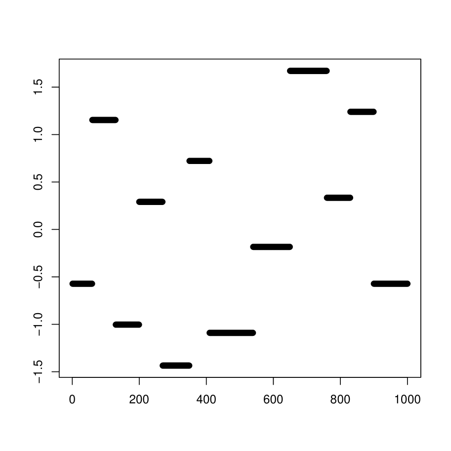
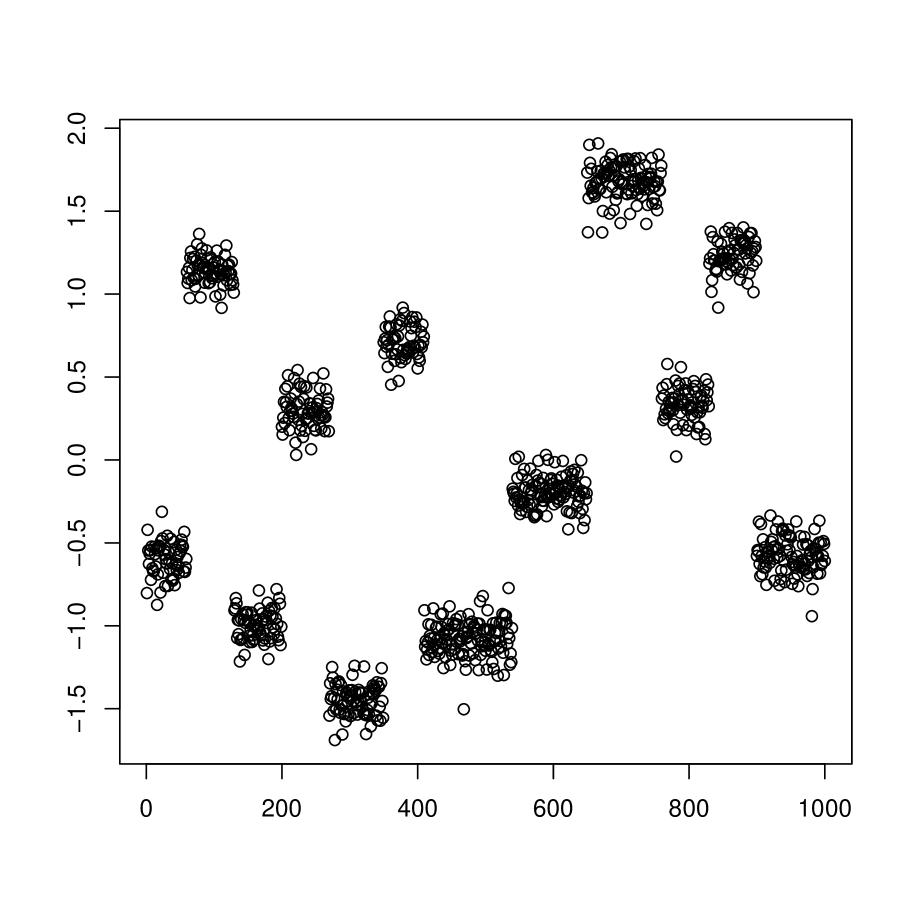
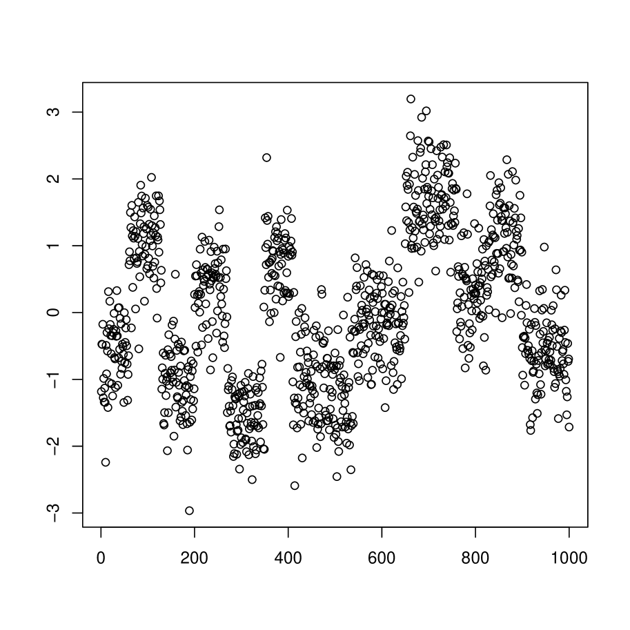
Figure S.1: Typical realization of the block model. Left: no noise ($\sigma=0$); Middle: medium noise ($\sigma=0.1$); Right: high noise ($\sigma=0.5$).

Table S.10: Performance of SNM and LASSO under block models with different noise levels $\sigma$ and temporal dependence levels $\rho$.

			$\hat{m}-m_{o}$
Method	$\sigma$	$\rho$	$\leq-3$	$-2$	$-1$	$0$	$1$	$2$	$\geq 3$	ARI	$d_{1}\times 10^{2}$	$d_{2}\times 10^{2}$	$d_{H}\times 10^{2}$	time
SNM	0.1	0.0	0	0	0	999	1	0	0	0.989	0.11	0.10	0.11	3.82
LASSO	0.1	0.0	3	22	60	134	199	194	388	0.627	3.29	12.99	12.99	3.36
SNM	0.1	0.5	0	0	0	996	4	0	0	0.988	0.14	0.11	0.14	3.90
LASSO	0.1	0.5	4	30	67	133	173	157	436	0.627	3.30	12.99	12.99	3.40
SNM	0.5	0.0	0	0	45	954	1	0	0	0.973	0.32	0.62	0.63	3.86
LASSO	0.5	0.0	26	51	122	162	179	166	294	0.647	3.29	11.93	11.93	3.34
SNM	0.5	0.5	10	110	450	429	1	0	0	0.916	0.57	4.54	4.55	3.88
LASSO	0.5	0.5	21	33	81	127	141	153	444	0.652	3.31	11.23	11.23	3.35

S.2.2.2 Multivariate mean change

We further compare the proposed nested local-window segmentation algorithm (i.e. SNM) with SN-WBS, SN-NOT, SN-SBS and SN-SNOT for multivariate mean change. Specifically, we consider models (M1), (M2) and (M3) with $d=5$ and $d=10$, as in Section 4.2 of the main text. To conserve space, we only report the performance of SN-WBS², SN-NOT², SN-SBS² and SN-NOT². The performance of SN-WBS¹, SN-NOT¹, SN-SBS¹ and SN-NOT¹ are similar but slightly worse.

Table S.11 gives the estimation result for $d=5$ and Table S.12 summarizes the result for $d=10$. In general, the observation is the same as the one for univariate mean. Specifically, SNM provides comparable (or more favorable) performance as SN-WBS, SN-NOT, SN-SBS and SN-SNOT. For (M1) and (M2), SNM indeed provides notably better performance.

Table S.11: Performance of SNM, SN-WBS, SN-NOT, SN-SBS, SN-SNOT under change in multivariate mean with $d=5$.

		$\hat{m}-m_{o}$
Method	Model	$\leq-3$	$-2$	$-1$	$0$	$1$	$2$	$\geq 3$	ARI	$d_{1}\times 10^{2}$	$d_{2}\times 10^{2}$	$d_{H}\times 10^{2}$	time
SNM		0	0	13	946	41	0	0	0.953	1.16	1.12	1.37	12.48
SN-WBS2		0	0	12	802	178	8	0	0.950	1.94	1.10	2.15	146.87
SN-NOT2	$(M1)$	0	0	11	826	156	7	0	0.944	2.16	1.41	2.36	146.87
SN-SBS2		0	1	34	648	255	54	8	0.934	2.96	1.78	3.68	50.01
SN-SNOT2		0	1	37	694	224	39	5	0.926	3.11	2.28	3.84	50.01
SNM		0	11	175	628	166	18	2	0.937	4.59	1.93	5.68	22.88
SN-WBS2		0	6	71	380	338	152	53	0.854	11.85	1.65	12.17	291.21
SN-NOT2	$(M2)$	0	7	72	395	341	140	45	0.852	11.89	1.85	12.21	291.21
SN-SBS2		0	1	13	106	259	244	377	0.737	20.89	1.23	20.97	97.32
SN-SNOT2		0	1	12	108	260	246	373	0.734	20.90	1.47	20.98	97.32
SNM		0	0	4	993	3	0	0	0.968	0.93	0.96	1.03	60.00
SN-WBS2		0	0	4	992	4	0	0	0.966	1.01	1.02	1.10	829.59
SN-NOT2	$(M3)$	0	0	4	992	4	0	0	0.967	1.02	1.04	1.12	829.59
SN-SBS2		0	0	14	985	1	0	0	0.962	1.02	1.33	1.35	258.03
SN-SNOT2		0	0	13	986	1	0	0	0.967	0.91	1.21	1.23	258.03

Table S.12: Performance of SNM, SN-WBS, SN-NOT, SN-SBS, SN-SNOT under change in multivariate mean with $d=10$.

		$\hat{m}-m_{o}$
Method	Model	$\leq-3$	$-2$	$-1$	$0$	$1$	$2$	$\geq 3$	ARI	$d_{1}\times 10^{2}$	$d_{2}\times 10^{2}$	$d_{H}\times 10^{2}$	time
SNM		0	0	9	835	142	13	1	0.945	1.92	1.19	2.08	24.79
SN-WBS2		0	0	10	520	324	118	28	0.925	3.93	1.37	4.20	315.41
SN-NOT2	$(M1)$	0	1	15	574	296	99	15	0.905	4.15	2.20	4.45	315.41
SN-SBS2		0	5	51	377	349	163	55	0.892	5.18	3.14	6.59	98.97
SN-SNOT2		0	5	66	441	348	110	30	0.871	5.29	4.18	6.79	98.97
SNM		0	4	22	283	330	250	111	0.802	15.32	1.38	15.50	48.95
SN-WBS2		0	0	0	7	52	104	837	0.564	27.58	1.42	27.58	651.82
SN-NOT2	$(M2)$	0	0	1	7	50	135	807	0.559	27.56	2.15	27.56	651.82
SN-SBS2		0	0	0	0	0	0	1000	0.373	34.93	0.98	34.93	205.36
SN-SNOT2		0	0	0	0	0	0	1000	0.369	34.92	1.39	34.92	205.36
SNM		0	0	16	983	1	0	0	0.966	0.90	1.26	1.29	136.20
SN-WBS2		0	0	25	975	0	0	0	0.961	0.96	1.58	1.58	1870.29
SN-NOT2	$(M3)$	0	0	26	974	0	0	0	0.962	0.96	1.59	1.59	1870.29
SN-SBS2		0	0	46	954	0	0	0	0.955	0.95	2.09	2.09	565.24
SN-SNOT2		0	0	45	955	0	0	0	0.957	0.95	2.05	2.05	565.24

S.2.3 No change

Table S.13 reports the performance of SNCP and comparison methods under the null for $n=512$. Since the sample size $n=512$ is small, we set the window size $\epsilon=0.1$ for SNCP to ensure we have sufficient observations in each local-window. All implementations are the same as Table 2 in the main text. As can be seen, SNCP in general gives decent performance (i.e. achieving the target size at 10%) except for $\rho=0.8$, which is understandable as the effective sample size is low for strong positive temporal dependence.

Table S.13: Performance under no change-point scenario with $m_{o}=0$.

$n=512$	$\rho=-0.8$			$\rho=-0.5$			$\rho=0$			$\rho=0.5$			$\rho=0.8$
$\hat{m}$	$0$	$1$	$\geq 2$	$0$	$1$	$\geq 2$	$0$	$1$	$\geq 2$	$0$	$1$	$\geq 2$	$0$	$1$	$\geq 2$
SN90M	0.99	0.01	0.00	0.96	0.04	0.00	0.92	0.07	0.00	0.89	0.10	0.01	0.72	0.23	0.06
BP	1.00	0.00	0.00	1.00	0.00	0.00	0.98	0.01	0.00	0.26	0.12	0.62	0.00	0.00	1.00
SN90V	0.84	0.14	0.01	0.91	0.09	0.00	0.93	0.07	0.00	0.87	0.12	0.01	0.75	0.21	0.04
KF	0.32	0.25	0.44	0.69	0.21	0.11	0.81	0.12	0.06	0.83	0.12	0.05	0.83	0.12	0.05
MSML	0.48	0.34	0.19	0.76	0.21	0.04	0.83	0.15	0.01	0.84	0.14	0.01	0.84	0.14	0.01

S.2.4 Change in multivariate mean

Table S.14 reports the performance of SNM and CUSUM under change in multivariate mean with $d=10$. Compared to Table 3 in the main text (with $d=1$ and $5$), it can be seen that the performance of SNM and CUSUM both deteriorate due to the increasing dimension $d$. However, the deterioration of CUSUM is much more notable while SNM still gives decent performance as measured by ARI and $d_{H}$.

Table S.14: Performance of SNM and CUSUM under change in multivariate mean with $d=10$.

		$\hat{m}-m_{o}$
Method	Model	$\leq-3$	$-2$	$-1$	$0$	$1$	$2$	$\geq 3$	ARI	$d_{1}\times 10^{2}$	$d_{2}\times 10^{2}$	$d_{H}\times 10^{2}$	time
SNM	$(M1)$	0	0	9	835	142	13	1	0.945	1.92	1.19	2.08	24.79
CUSUM		242	9	2	186	287	192	82	0.695	4.79	15.47	19.19	0.04
SNM	$(M2)$	0	4	22	283	330	250	111	0.802	15.32	1.38	15.50	48.95
CUSUM		49	13	15	19	57	157	690	0.505	23.29	5.64	25.54	0.10
SNM	$(M3)$	0	0	16	983	1	0	0	0.966	0.90	1.26	1.29	136.20
CUSUM		0	617	1	381	1	0	0	0.367	0.47	31.34	31.35	0.07

S.2.5 Change in variance

For variance change, we consider four univariate time series $\{Y_{t}\}_{t=1}^{n}$ with piecewise constant variance. (V1) is an AR(1) process with moderate temporal dependence adapted from Cho and Fryzlewicz, (2012). (V2) is an ARMA(1,1) process taken from Korkas and Fryzlewicz, (2017). (V3) is an AR(2) process with strong positive dependence taken from Cho and Fryzlewicz, (2012). (V4) is an AR(1) process with longer segments and only one small-scale change. Typical realizations of (V1)-(V4) can be found in Figure S.2 of the supplementary material.

$$\text{(V1)}:n=1024,~{}~{}Y_{t}=\begin{cases}0.5Y_{t-1}+\epsilon_{t},&t\in[1,400],\\ 0.5Y_{t-1}+2\epsilon_{t},&t\in[401,750],\\ 0.5Y_{t-1}+\epsilon_{t},&t\in[751,1024].\end{cases}$$

$$\text{(V2)}:n=1024,~{}~{}Y_{t}=\begin{cases}0.7Y_{t-1}+\epsilon_{t}+0.6\epsilon_{t-1},&t\in[1,125],\\ 0.3Y_{t-1}+\epsilon_{t}+0.3\epsilon_{t-1},&t\in[126,532],\\ 0.9Y_{t-1}+\epsilon_{t},&t\in[533,704],\\ 0.1Y_{t-1}+\epsilon_{t}-0.5\epsilon_{t-1},&t\in[705,1024].\end{cases}$$

$$\text{(V3)}:n=1024,~{}~{}Y_{t}=\begin{cases}0.9Y_{t-1}+\epsilon_{t},&t\in[1,512],\\ 1.69Y_{t-1}-0.81Y_{t-2}+\epsilon_{t},&t\in[513,768],\\ 1.32Y_{t-1}-0.81Y_{t-2}+\epsilon_{t},&t\in[769,1024].\end{cases}$$

$$\text{(V4)}:n=2048,~{}~{}Y_{t}=\begin{cases}-0.7Y_{t-1}+\epsilon_{t},&t\in[1,1024],\\ -0.7Y_{t-1}+\sqrt{2}\epsilon_{t},&t\in[1025,2048].\end{cases}$$

The error process $\{\epsilon_{t}\}$ is i.i.d. standard normal $N(0,1)$.

The estimation result is summarized in Table S.15. For (V1), under moderate temporal dependence, all methods give decent performance with some degree of over-estimation. For (V2), due to the complex dependence, all methods experience power loss, especially for KF and SNV, with MSML giving the best performance. For (V3), due to the strong positive dependence, SNV and KF again experience power loss, with SNV giving noticeably larger estimation error. For (V4), under strong negative dependence, KF and MSML severely over-estimate the number of change-points while SNV gives robust and best performance. In summary, SNV performs quite well compared to MSML and KF, though it may exhibit some lack of power under strong positive dependence $(\rho\geq 0.9)$.

Table S.15: Performance of SNV, KF, MSML under change in variance.

		$\hat{m}-m_{o}$
Method	Model	$\leq-3$	$-2$	$-1$	$0$	$1$	$2$	$\geq 3$	ARI	$d_{1}\times 10^{2}$	$d_{2}\times 10^{2}$	$d_{H}\times 10^{2}$
SNV		0	0	5	938	53	4	0	0.942	2.09	1.49	2.26
KF	$(V1)$	0	0	0	963	35	2	0	0.958	1.70	1.09	1.70
MSML		0	0	0	892	102	6	0	0.957	2.84	0.96	2.84
SNV		12	95	335	538	18	2	0	0.762	2.94	17.35	17.50
KF	$(V2)$	0	121	397	463	17	2	0	0.730	3.30	17.53	17.73
MSML		0	19	161	674	137	7	2	0.792	5.49	8.49	9.46
SNV		0	37	315	542	94	12	0	0.733	6.76	13.65	15.99
KF	$(V3)$	0	0	129	543	258	60	10	0.853	6.52	7.44	9.94
MSML		0	0	1	638	295	58	8	0.883	8.23	3.53	8.26
SNV		0	0	38	898	58	6	0	0.870	3.66	4.03	5.56
KF	$(V4)$	0	0	0	315	219	246	220	0.769	22.35	1.33	22.35
MSML		0	0	0	439	345	154	62	0.834	17.68	1.58	17.68

S.2.6 Change in autocorrelation

For autocorrelation change, we generate three univariate time series $\{Y_{t}\}_{t=1}^{n}$ with piecewise constant autocorrelation. (A1) and (A2) are AR(1) processes taken from Cho and Fryzlewicz, (2012). (A3) is an ARMA(1,1) process adapted from Korkas and Fryzlewicz, (2017). Typical realizations of (A1)-(A3) can be found in Figure S.2 of the supplementary material.

$$\text{(A1)}:n=1024,~{}~{}Y_{t}=\begin{cases}0.5Y_{t-1}+\epsilon_{t},&t\in[1,400],\\ 0.9Y_{t-1}+\epsilon_{t},&t\in[401,750],\\ 0.3Y_{t-1}+\epsilon_{t},&t\in[751,1024].\end{cases}$$

$$\text{(A2)}:n=1024,~{}~{}Y_{t}=\begin{cases}0.75Y_{t-1}+\epsilon_{t},&t\in[1,50],\\ -0.5Y_{t-1}+\epsilon_{t},&t\in[51,1024].\end{cases}$$

$$\text{(A3)}:n=1024,~{}~{}Y_{t}=\begin{cases}-0.9Y_{t-1}+\epsilon_{t}+0.7\epsilon_{t-1},&t\in[1,512],\\ 0.9Y_{t-1}+\epsilon_{t},&t\in[513,768],\\ \epsilon_{t}-0.7\epsilon_{t-1},&t\in[769,1024].\end{cases}$$

The error process $\{\epsilon_{t}\}$ is i.i.d. standard normal $N(0,1)$.

The estimation result is summarized in Table S.16. For (A1), SNA gives the best performance while both KF and MSML seem to suffer power loss. For (A2), the change-point location is close to the boundary with $\tau_{1}=50/1024<0.05=\epsilon$, violating the assumption of SNA. However, SNA still delivers arguably the best performance as measured by ARI. For (A3), all methods tend to over-estimate with SNA providing the most robust performance. In summary, SNA performs favorably compared to MSML and KF for detecting autocorrelation changes in the time series. On the other hand, SNA is computationally more expensive than KF and MSML, since the latter two methods are built on fast wavelet transformation.

Table S.16: Performance of SNA, KF, MSML under change in autocorrelation.

		$\hat{m}-m_{o}$
Method	Model	$\leq-3$	$-2$	$-1$	$0$	$1$	$2$	$\geq 3$	ARI	$d_{1}\times 10^{2}$	$d_{2}\times 10^{2}$	$d_{H}\times 10^{2}$	time
SNA		0	2	69	907	20	2	0	0.895	2.17	4.22	4.56	18.84
KF	$(A1)$	0	135	107	728	27	3	0	0.650	5.34	15.99	16.37	0.29
MSML		0	131	71	654	139	4	1	0.699	5.94	12.99	15.06	0.01
SNA		0	0	59	741	170	29	1	0.724	11.23	4.39	14.18	19.03
KF	$(A2)$	0	0	143	668	118	58	13	0.548	13.10	11.87	20.25	0.40
MSML		0	0	7	769	201	20	3	0.673	12.47	2.02	12.82	0.01
SNA		0	0	0	831	150	16	3	0.940	4.55	0.57	4.55	18.82
KF	$(A3)$	0	0	0	638	222	118	22	0.885	9.57	1.08	9.57	0.30
MSML		0	0	0	665	258	69	8	0.870	9.35	2.26	9.35	0.02

S.2.7 Change in correlation

For correlation change, we generate two bivariate time series $\{Y_{t}=(Y_{t1},Y_{t2})\}_{t=1}^{n}$ with $n=1000$ using piecewise constant correlation. Denote $\Sigma_{r}=[1,r;r,1]$, we define

$$\text{(R0)}:Y_{t}=0.5\mathbf{I}_{2}Y_{t-1}+\mathbf{e}_{t},~{}\mathbf{e}_{t}\overset{i.i.d.}{\sim}N(0,\Sigma_{0.5}),t\in[1,1000].$$

$$\text{(R1)}:Y_{t}=\begin{cases}0.5\mathbf{I}_{2}Y_{t-1}+2\mathbf{e}_{t},~{}~{}\mathbf{e}_{t}\overset{i.i.d.}{\sim}N(0,\Sigma_{0.8}),&t\in[1,333],\\ 0.5\mathbf{I}_{2}Y_{t-1}+\mathbf{e}_{t},~{}~{}\mathbf{e}_{t}\overset{i.i.d.}{\sim}N(0,\Sigma_{0.2}),&t\in[334,667],\\ 0.5\mathbf{I}_{2}Y_{t-1}+\mathbf{e}_{t},~{}~{}\mathbf{e}_{t}\overset{i.i.d.}{\sim}N(0,\Sigma_{0.8}),&t\in[668,1000].\end{cases}$$

$$\text{(R2)}:Y_{t}=\begin{cases}0.5\mathbf{I}_{2}Y_{t-1}+\sqrt{2}\mathbf{e}_{t},~{}~{}\mathbf{e}_{t}\overset{i.i.d.}{\sim}N(0,\Sigma_{0.8}),&t\in[1,333],\\ 0.5\mathbf{I}_{2}Y_{t-1}+\mathbf{e}_{t},~{}~{}\mathbf{e}_{t}\overset{i.i.d.}{\sim}N(0,\Sigma_{0.2}),&t\in[334,667],\\ 0.5\mathbf{I}_{2}Y_{t-1}+2\mathbf{e}_{t},~{}~{}\mathbf{e}_{t}\overset{i.i.d.}{\sim}N(0,\Sigma_{0.2}),&t\in[668,1000].\end{cases}$$

For (R1), the correlation changes from 0.8 to 0.2 and back to 0.8. At the first change-point $t=333$, the variance of the time series also changes. For (R2), the correlation only changes once from 0.8 to 0.2 at $t=333$. At $t=667$, the covariance matrix changes but the correlation remains the same.

The estimation result is reported in Table S.17. For (R1), SNC gives noticeably better performance with much higher ARI and lower Hausdorff distance, while GW seems to over-estimate and experience power loss at the same time. The power loss of GW is due to its inability to detect the first change-point, where correlation change comes with large variance change. For (R2), SNC again outperforms GW. Note that GW systematically over-estimates the number of change-points as it mistakenly detects the sole variance change at $t=667$ as correlation change. For (R0), both methods give decent performance with SNC achieving the target size perfectly. In summary, SNC performs favorably and retains size and power for detecting change in correlation when other quantities such as variance also experience structural breaks.

Table S.17: Performance of SNC, GW under change in correlation of bivariate time series.

		$\hat{m}-m_{o}$
Method	Model	$\leq-3$	$-2$	$-1$	$0$	$1$	$2$	$\geq 3$	ARI	$d_{1}\times 10^{2}$	$d_{2}\times 10^{2}$	$d_{H}\times 10^{2}$	time
SNC	$(R1)$	0	0	9	941	50	0	0	0.937	2.06	1.76	2.35	22.43
GW		0	376	0	440	159	17	8	0.558	3.88	20.03	22.68	0.28
Method	Model	$\leq-3$	$-2$	$-1$	$0$	$1$	$2$	$\geq 3$	ARI	$d_{1}\times 10^{2}$	$d_{2}\times 10^{2}$	$d_{H}\times 10^{2}$	time
SNC	$(R2)$	0	0	0	916	80	4	0	0.932	3.23	1.05	3.23	22.78
GW		0	0	0	11	471	328	190	0.522	31.15	1.24	31.15	0.49
Method	Model	$\hat{m}=0$	$\hat{m}=1$	$\hat{m}\geq 2$
SNC	$(R0)$	900	90	10
GW		892	80	28

S.2.8 Change in quantile

To our best knowledge, SNQ is the only nonparametric method available for detecting structural breaks in quantiles under temporal dependence. Note that there is a stream of literature on testing and estimating structural breaks in quantile regressions, see Qu, (2008), Oka and Qu, (2011) and Aue et al., (2014). However, in all these papers, a parametric linear quantile form is typically specified and the error in the location-scale quantile regression model is assumed to be i.i.d., which does not cover the nonparametric time series setting we are focusing on here.

For illustration, we compare SNQ with the recently proposed multiscale quantile segmentation (MQS) in Vanegas et al., (2021), which is a nonparametric method designed for detecting piecewise constant quantile changes under a temporal independence assumption. In addition, we compare with ECP in Matteson and James, (2014), which is a nonparametric method designed for detecting distributional changes based on the energy statistics. We emphasize that the comparison is not completely fair as the validity of MQS and ECP require temporal independence.

A stylized fact of financial markets is that upper quantiles of negative log-returns (i.e. losses) of stocks are subject to more changes than lower quantiles. Based on a mixture of a truncated normal distribution and a generalized Pareto distribution (GPD), we design a univariate time series to resemble such phenomenon. GPD is a commonly used distribution for characterizing high quantiles of financial returns, see Embrechts et al., (1997). Denote $\Phi(\cdot)$ as the CDF of $N(0,1)$, we use a standard normal distribution truncated at 0 with CDF $F_{1}(x)=2\Phi(x),x\leq 0$. The CDF of a GPD distribution takes the form $F_{2}(x)=1-(1+\xi(x-\mu)/\sigma)_{+}^{-1/\xi}$, where we set the location parameter $\mu=0$, scale parameter $\sigma=2$ and tail index $\xi=0.125$. Setting the mixture as $F(x)=0.5F_{1}(x)+0.5F_{2}(x)$, it is easy to see that $F(x)$ is a continuous distribution with $F^{-1}(q)=\Phi^{-1}(q)$ for $q\leq 0.5$.

To introduce temporal dependence, we first simulate a stationary univariate time series $\{X_{t}\}_{t=1}^{n}$ from an AR(1) process with $X_{t}=\rho X_{t-1}+\sqrt{1-\rho^{2}}\epsilon_{t},$ where $\rho=0.2$ and $\{\epsilon_{t}\}$ is i.i.d. $N(0,1)$. Thus $\{u_{t}=\Phi(X_{t})\}_{t=1}^{n}$ is a stationary time series with uniform margins. Based on $F(x)$ and $\{u_{t}\}_{t=1}^{n}$, we define $\{Y_{t}\}_{t=1}^{n}$ such that

$$\text{(Q1)}:n=1000,~{}~{}Y_{t}=\begin{cases}\Phi^{-1}(u_{t}),&t\in[1,500],\\ F^{-1}(u_{t}),&t\in[501,1000].\end{cases}$$

A typical realization of (Q1) can be found in Figure S.2 of the supplementary material.

We use SNQ and MQS to detect change-points in the 10% quantile (no change-point) and 90% quantile (one change-point) of $\{Y_{t}\}_{t=1}^{n}$ respectively. Note that ECP cannot be tailored to detect changes in a specific quantile level, thus we can only apply it to detect if there is any distributional change in the data (one change-point). The estimation result is reported in Table S.18. For (Q1) 90% quantile, SNQ gives notably better performance with much higher ARI and lower Hausdorff distance, while MQS seems to severely over-estimate. For (Q1) 10% quantile, the size of SNQ is close to the target size of 10%, while MQS yields over-detection of change-points. As for ECP, it always estimates at least one change-point as it targets distributional change and tends to over-estimate due to intolerance to temporal dependence.

In summary, SNQ performs fairly well for quantile change detection while ignoring temporal dependence can lead to less favorable results for MQS. In addition, compared to algorithms that target distributional changes such as ECP, SNCP can be tailored to detect changes in a specific parameter and thus provides more information about the nature of change, e.g. whether the change stems from the lower 10% quantile or the upper 90% quantile.

Table S.18: Performance of SNQ, MQS under change in quantile.

		$\hat{m}-m_{o}$
Method	Model	$\leq-3$	$-2$	$-1$	$0$	$1$	$2$	$\geq 3$	ARI	$d_{1}\times 10^{2}$	$d_{2}\times 10^{2}$	$d_{H}\times 10^{2}$	time
SNQ		0	0	4	903	84	9	0	0.911	3.99	1.94	4.19	25.64
MQS	$(Q1)$-90%	0	0	0	594	221	115	70	0.746	15.19	4.01	15.19	509.27
ECP		0	0	0	658	168	125	49	0.842	11.46	2.11	11.46	17.64
Method	Model	$\hat{m}=0$	$\hat{m}=1$	$\hat{m}\geq 2$
SNQ		860	122	18
MQS	$(Q1)$-10%	462	313	225
ECP		0	658	342

S.2.9 Simultaneous change in mean and variance

In this section, we further investigate the robustness of SNM and SNV under the scenario where both mean and variance change at the same time. We first simulate a stationary univariate time series $\{X_{t}\}_{t=1}^{n}$ from an AR(1) process such that $X_{t}=\rho X_{t-1}+\epsilon_{t},$ where $\{\epsilon_{t}\}$ is i.i.d. $N(0,1)$. We then generate two different time series $\{Y_{t}\}_{t=1}^{n}$ with piecewise constant mean and variance based on $\{X_{t}\}_{t=1}^{n}$.

$$\text{(MV1)}:n=1024,~{}~{}\rho=0.5,~{}~{}Y_{t}=\begin{cases}0+X_{t},&t\in[1,512],\\ 1+1.5X_{t},&t\in[513,1024].\end{cases}$$

$$\text{(MV2)}:n=1024,~{}~{}\rho=-0.5,~{}~{}Y_{t}=\begin{cases}0+X_{t},&t\in[1,512],\\ 1+1.5X_{t},&t\in[513,1024].\end{cases}$$

We run (SNM, BP) and (SNV, KF, MSML) on $\{Y_{t}\}_{t=1}^{n}$. The estimation result is summarized in Table S.19. In general, the observation is as follows. SNM and BP are robust against change in variance. Additionally, BP suffers severe over-estimation under positive dependence. SNV, KF, MSML are robust against change in mean while MSML tends to over-estimate.

Table S.19: Estimation result under change in mean and variance.

		$\hat{m}-m_{o}$
Method	Model	$\leq-3$	$-2$	$-1$	$0$	$1$	$2$	$\geq 3$	ARI	$d_{1}\times 10^{2}$	$d_{2}\times 10^{2}$	$d_{H}\times 10^{2}$	time
SNM		0	0	49	862	81	8	0	0.852	4.24	4.64	6.69	4.02
BP	$(MV1)$	0	0	0	267	174	229	330	0.715	24.54	2.20	24.54	37.12
SNV		0	0	27	887	80	6	0	0.887	3.87	3.18	5.22	17.80
KF	$(MV1)$	0	0	1	956	37	6	0	0.935	2.59	1.57	2.64	0.24
MSML		0	0	0	743	250	7	0	0.908	6.62	1.35	6.62	0.02
SNM		0	0	0	980	20	0	0	0.976	0.92	0.49	0.92	3.99
BP	$(MV2)$	0	0	0	1000	0	0	0	0.990	0.25	0.25	0.25	37.40
SNV		0	0	32	913	54	1	0	0.890	3.12	3.39	4.72	17.76
KF	$(MV2)$	0	0	0	809	135	51	5	0.906	6.47	1.62	6.47	0.29
MSML		0	0	0	723	236	40	1	0.883	8.28	1.92	8.28	0.02

S.2.10 Change in covariance matrix

In this section, we consider two additional simulation settings for changes in covariance matrix of a VAR process. Specifically, we consider change in covariance matrices of a four-dimensional time series $\{Y_{t}=(Y_{t1},\cdots,Y_{t4})\}_{t=1}^{n}$ with $n=1000$. Denote $\Sigma_{\rho}$ as an exchangeable covariance matrix with unit variance and equal covariance $\rho$, we consider

$$\text{(C3)}:Y_{t}=\begin{cases}0.3\mathbf{I}_{4}Y_{t-1}+\sqrt{2}\mathbf{e}_{t},~{}~{}\mathbf{e}_{t}\overset{i.i.d.}{\sim}N(0,\Sigma_{0.5}),&t\in[1,333],\\ 0.3\mathbf{I}_{4}Y_{t-1}+\mathbf{e}_{t},~{}~{}\mathbf{e}_{t}\overset{i.i.d.}{\sim}N(0,\Sigma_{0.2}),&t\in[334,667],\\ 0.3\mathbf{I}_{4}Y_{t-1}+\sqrt{2}\mathbf{e}_{t},~{}~{}\mathbf{e}_{t}\overset{i.i.d.}{\sim}N(0,\Sigma_{0.5}),&t\in[668,1000].\end{cases}$$

$$\text{(C4)}:Y_{t}=\begin{cases}0.3\mathbf{I}_{4}Y_{t-1}+\mathbf{e}_{t},~{}~{}\mathbf{e}_{t}\overset{i.i.d.}{\sim}N(0,\Sigma_{0.2}),&t\in[1,333],\\ 0.3\mathbf{I}_{4}Y_{t-1}+\sqrt{2}\mathbf{e}_{t},~{}~{}\mathbf{e}_{t}\overset{i.i.d.}{\sim}N(0,\Sigma_{0.5}),&t\in[334,667],\\ 0.3\mathbf{I}_{4}Y_{t-1}+2\mathbf{e}_{t},~{}~{}\mathbf{e}_{t}\overset{i.i.d.}{\sim}N(0,\Sigma_{0.5}),&t\in[668,1000].\end{cases}$$

(C3) and (C4) generate covariance changes in the VAR model, which is widely used in the time series literature. The estimation result is reported in Table S.20. For monotonic changes (C4), both methods perform well though AHHR tends to over-estimate the number of change-points, while for non-monotonic changes (C3), AHHR seems to over-estimate and experience power loss at the same time and is outperformed by SNCM.

Table S.20: Performance of SNCM and AHHR under change in covariance matrix.

		$\hat{m}-m_{o}$
Method	Model	$\leq-3$	$-2$	$-1$	$0$	$1$	$2$	$\geq 3$	ARI	$d_{1}\times 10^{2}$	$d_{2}\times 10^{2}$	$d_{H}\times 10^{2}$	time
SNCM	$(C3)$	0	0	51	912	37	0	0	0.904	2.36	3.66	4.06	56.50
AHHR		0	525	8	342	104	18	3	0.408	2.84	27.95	29.32	0.37
SNCM	$(C4)$	0	0	19	947	33	1	0	0.924	2.22	2.42	2.85	56.96
AHHR		0	0	8	780	175	33	4	0.883	5.27	3.00	5.53	0.65

S.2.11 Change in multi-parameter

In this section, we consider an additional simulation setting

$$\text{(MP3)}:n=1000,~{}~{}~{}Y_{t}=\begin{cases}0.1Y_{t-1}+\epsilon_{t},&t\in[1,333],\\ 0.6Y_{t-1}+\epsilon_{t},&t\in[334,667],\\ 0.1Y_{t-1}+\epsilon_{t},&t\in[668,1000].\end{cases}$$

Here $\{\epsilon_{t}\}_{t=1}^{n}$ is i.i.d. $N(0,1)$. Thus the change in $\{Y_{t}\}_{t=1}^{n}$ is driven by autocorrelation and further affects the variance of the marginal distribution of $Y_{t}$.

The estimation result is summarized in Table S.21. As can be seen, SNA gives decent performance as the change originates from autocorrelation. Including variance and quantile in the multi-parameter set improves the estimation accuracy of SNMP, but only by a small amount. On the other hand, ECP does not perform well, possibly due to the strong temporal dependence in the second segment of $\{Y_{t}\}_{t=1}^{n}$.

Table S.21: Performance of SNMP and ECP under change in multi-parameter.

		$\hat{m}-m_{o}$
Method	Model	$\leq-3$	$-2$	$-1$	$0$	$1$	$2$	$\geq 3$	ARI	$d_{1}\times 10^{2}$	$d_{2}\times 10^{2}$	$d_{H}\times 10^{2}$	time
SNA		0	7	86	870	37	0	0	0.873	2.72	5.29	5.80	11.32
SNVA	$(MP3)$	0	2	49	884	64	1	0	0.898	2.80	3.62	4.44	26.88
SNVAQ90		0	1	70	841	83	5	0	0.881	3.27	4.49	5.50	49.87
ECP		0	126	24	245	212	211	182	0.512	12.22	17.61	21.59	12.28

S.2.12 Implementation details of comparison methods and typical realizations of DGP used in simulation

All implementations of the comparison methods are set to the recommended settings by the corresponding papers or R packages. We believe the default settings of the papers or R packages accommodate the presence of serial correlations as the methods we compare with are explicitly designed to handle temporal dependence. The only exceptions are ECP in Matteson and James, (2014) for distributional change and MQS in Vanegas et al., (2021) for quantile change, which can only handle temporal independence, as we cannot find methods for distributional or quantile change that can accommodate temporal dependence.

Note that for all simulation experiments in Section 4 of the main text and in Section S.2 of the supplement, except CUSUM, which is simple enough to be coded by ourselves, all the other competing methods are implemented using source codes obtained from the authors’ website or from the corresponding R packages.

For CUSUM, we estimate the long-run variance following the recommendation in Aue et al., (2009), which uses a Bartlett kernel with bandwidth $\log_{10}n$. For BP in Bai and Perron, (2003) it is implemented via function breakpoints() in the R package strucchange. For MSML in Cho and Fryzlewicz, (2012), it is implemented via source code from Dr. Haeran Cho’s website. For KF in Korkas and Fryzlewicz, (2017), it is implemented via function wbs.lsw() in the R package wbsts. For GW in Wied et al., (2012) and Galeano and Wied, (2017), it is implemented via source code from Dr. Dominik Wied’s website. For ECP in Matteson and James, (2014), it is implemented via function e.divisive() in the R package ecp. For MQS in Vanegas et al., (2021), it is implemented via function mqse() in the R package mqs.

Figure S.2: Typical realizations of DGP used in simulation.

S.3 Real Data Applications

S.3.1 Change-point detection in climate data

In this section, we analyze two climate datasets using SNCP to illustrate the evidence of climate change. The first dataset contains the annual mean temperature of central England from 1772 to 2019, covering $n=247$ years in total. We apply SNM and BP to detect possible mean change in the time series and the estimation result is given in Figure S.3(a). SNM detects two change-points at 1919 and 1988 and BP gives two changes at 1910 and 1988. In addition, we apply ECP, which detects two change-points at 1926 and 1988. Based on the estimated change-points by SNM, the expected annual mean temperature is 9.15^∘C from 1772-1919, 9.52^∘C from 1920-1988, and 10.25^∘C from 1989-now, which clearly indicates the trend of global warming.

The second dataset contains the satellite-derived lifetime-maximum wind speeds of $n=2098$ tropical cyclones over the globe during 1981–2006, and we refer to Elsner et al., (2008) for a more detailed description. It is known in climate science that intensity of tropical cyclones increases with rising ocean temperature, one of the major consequences of global warming. As a result, researchers have been seeking empirical evidence on changes in tropical cyclone wind speeds, see Elsner et al., (2008), Zhang and Wu, (2011), Zhang and Lavitas, (2018) and references therein. Specifically, the change-point test in Zhang and Lavitas, (2018) indicates strong evidence of mean change in the time series of maximum wind speed, however, their test is incapable of locating the exact change-point. We apply SNM and BP to locate the possible change-points in mean. Surprisingly, BP fails to detect any change, while SNM detects one change-point at 1988 with an increase of maximum wind speed (see Figure S.3(b)). Interestingly, this aligns with the second estimated change-point in central England temperature, which provides further evidence of climate change. We also apply ECP, which detects one change-point at 1986, providing additional support for the finding based on SNM. The advantage of SNM here is that it not only detects the change but further indicates that the change is due to an increase in the mean level of maximum wind speed, which is more informative than ECP for the climate study.

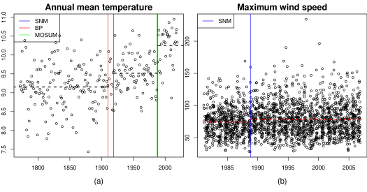
Figure S.3: (a) Estimated change-points for central England temperature. (b) Estimated change-points for cyclones maximum wind speed. Horizon dashed line indicates the sample mean of each segment by SNM.

S.3.2 Change-point detection in financial data

In this section, we study the behavior of financial markets using SNCP. A stylized fact in finance is that volatility of stock markets is much higher during crisis than normal periods. To validate this, we examine the volatility behavior of the S&P 500 index (hereafter SP500) for a period around the 2008 financial crisis. The data consist of daily (negative) log-returns of SP500 from June 2006 to December 2010 with $n=1024$ observations (to facilitate the implementation of MSML). Two widely used measures for (unconditional) volatility in financial markets are variance and Value-at-Risk (which is high quantile such as the 90% or 95% quantile), and they serve as basis for important applications such as portfolio optimization and systemic risk monitoring. Thus, it is crucial to study the structural breaks in these parameters.

We employ SNCP to detect changes in variance, 90% and 95% quantiles of daily (negative) log-returns of SP500, and their multi-parameter combination. Specifically, we implement seven SNCP based estimators: SNV, SNQ₉₀, SNQ₉₅, SNQ_90,95, SNQ₉₀V, SNQ₉₅V and SNQ_90,95V. Each estimator provides an assessment of volatility change in SP500. For comparison, we further apply MSML and KF, which target variance change and also apply ECP, which targets distributional change. The estimation result is summarized in Table S.22 and is further visualized in Figure S.4.

For variance change, SNV detects 4 change-points, MSML gives 6 changes and KF detects 5 changes. The estimated change-points by SNV, MSML and KF are close to each other. The three methods detect the inception of the financial crisis around July 2007, the acceleration of the crisis around September 2008, and the end of the crisis around May 2009. MSML and KF further detect changes in a relatively calm period from August 2006 to January 2007, which may be false positives or small-scale changes.

For high quantile change, both SNQ₉₀ and SNQ₉₅ detect 3 change-points at similar but different dates, around the inception, acceleration and end of the financial crisis, providing further evidence for volatility changes in the stock market during crisis. Moreover, the multi-parameter estimation given by SNQ_90,95 points to 3 changes at similar locations and further nicely reconciles the difference between SNQ₉₀ and SNQ₉₅, thus suggesting the robustness of our findings. Interestingly, ECP also gives 3 changes around similar time as the three SNQ estimators. However, the result given by SNQ is more informative as it further narrows down the changes to high quantiles.

The multi-parameter SN based on both high-quantile and variance (i.e. SNQ₉₀V, SNQ₉₅V, SNQ_90,95V) all detect 4 change-points at similar locations as SNV, which can be seen as evidence that the volatility changes due to variance detected by SNV is substantial and credible.

Table S.22: Estimated change-points by various SNCP estimators, MSML, KF and ECP for the S&P 500 index from June 2006 to December 2010.

	Method	CP1	CP2	CP3	CP4	CP5	CP6
	SNV			07/17/2007	09/16/2008	12/05/2008	05/27/2009
	MSML	07/28/2006	02/23/2007	07/18/2007	09/02/2008	12/01/2008	04/20/2009
	KF	08/01/2006	01/23/2007	07/23/2007	08/20/2008		04/20/2009
	ECP			07/20/2007	09/17/2008		04/21/2009
SP500	SNQ90			06/12/2007	08/04/2008		05/18/2009
	SNQ95			07/09/2007	09/17/2008		04/30/2009
	SNQ90,95			07/09/2007	09/17/2008		05/18/2009
	SNQ90V			07/17/2007	09/16/2008	12/05/2008	05/27/2009
	SNQ95V			07/09/2007	09/16/2008	12/08/2008	04/21/2009
	SNQ90,95V			07/09/2007	09/16/2008	12/05/2008	04/20/2009

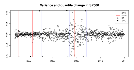
Figure S.4: Estimated change-points in variance by SNV, MSML, KF and estimated change-points in 90% quantile by SNQ for the S&P 500 index from June 2006 to December 2010.

The above analysis demonstrates the versatility and robustness of SNCP. It can be seamlessly applied to change-point detection for various parameters and provides reliable estimation results. In practice, the ground truth is unknown, thus it is important to examine the behavior change of the data via different angles. In this respect, the versatility of SNCP gives it a unique edge, as SNCP can provide practitioners the freedom to virtually examine any parameter of interest. With additional domain knowledge (e.g. examining volatility of financial markets via both variance and high quantiles), the practitioners can further design multi-parameter based SNCP to improve estimation accuracy, reconcile possibly different estimations given by SNCP for individual parameters, and conduct robustness check of the estimation results.

Another well-known hypothesis in the financial literature is that the international equity market correlation increases in volatile times and the correlation further increases due to the growing integration of the global economy (Longin and Solnik,, 2002; Poon et al.,, 2004).

To validate this hypothesis, we examine the correlation between daily (negative) log-returns of the S&P 500 index (U.S. market) and the DAX index (German market) for a 12-year period from January 2000 to December 2012 with $n=2684$ observations. We apply SNC and GW to detect potential changes in correlation. The estimation result is visualized in Figure S.5. SNC detects three change-points at 11/06/2003, 01/10/2006 and 10/20/2008. In contrast, GW detects one change-point at 10/21/2008.

The three change-points detected by SNC partition the 12-year period into 4 segments with Jan. 2000-Nov. 2003 ($\hat{\rho}=0.61$), Dec. 2003-Jan. 2006 ($\hat{\rho}=0.40$), Feb. 2006-Oct. 2008 ($\hat{\rho}=0.51$), and Nov. 2008-Dec. 2012 ($\hat{\rho}=0.70$). SP500 and DAX exhibit strong correlation during the first segment, which contains the period of the early 2000 recession and Dot-com bubble from 2000-2002. The correlation decreases to 0.40 after the crisis but starts to build up following the inception of the 2008 financial crisis and remains at a high level 0.70 during the post-crisis period. This result provides empirical evidence for the hypothesis in Longin and Solnik, (2002) and indicates that the systemic risk in the global financial market is increasing during the past decades.

We remark that since the ground truth is unknown, the estimation results given by SNC need to be interpreted and treated with caution. Here, we further provide some discussion about the discrepancy between the estimated change-points by SNC and GW. The magnitude of change in sample correlation at the first change-point ($\hat{\rho}=0.61$ to $0.40$) and the third change-point ($\hat{\rho}=0.51$ to $0.70$) estimated by SNC are rather significant, providing some evidence for the validity of the detected change-points; whereas the magnitude of change is smaller at the second change-point ($\hat{\rho}=0.40$ to $0.51$), suggesting it could be due to false positives as the threshold $K_{n}$ of SNC is set at the 90% critical level.

Note that around the first change-point (11/06/2003) estimated by SNC, the bivariate time series also experienced a significant change in its variance. This matches the simulation setting of (R1) in Section S.2.7 of the main text, where the simulation result suggests that GW tends to experience power loss for detecting correlation changes when there is large concurrent variance changes in the data. Indeed, the asymptotic validity of GW requires an approximately constant variance, see Assumptions (A4) and (A5) in Wied et al., (2012).

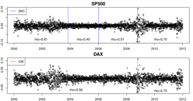
Figure S.5: Estimated change-points in correlation between the S&P 500 index and the DAX index by SNC (upper panel) and GW (lower panel) from January 2000 to December 2012.

S.4 Verification of Assumptions in Smooth Function Model

In this section, we derive explicit formulas for the partial influence function based expansion (5) and (3.2) in the main text, and provide detailed verification of Assumptions 2.1-2.3 and 3.1-3.3 for $\theta(\cdot)$ in the smooth function model, which includes a wide class of parameters such as mean, variance, (auto)-covariance and (auto)-correlation.

S.4.1 Verification of assumptions in Mean

By simple calculation, for any $\omega_{a,b}$, we have $\xi_{i}(Y_{t}^{(i)},\omega_{a,b})=Y_{t}^{(i)}-E(Y_{t}^{(i)})$, $i=1,2$ and $r_{a,b}(\omega_{a,b})\equiv 0$. Thus, Assumption 2.1 holds if the invariance principle holds jointly for the two stationary segments. Assumptions 2.2 and 2.3 hold trivially. Verification of Assumptions 3.1-3.3 is quite similar.

S.4.2 Verification of assumptions in Smooth Function Model

The smooth function model is a broad framework that covers important functionals such as mean, variance, (auto)-covariance and (auto)-correlation (Bhattacharya et al.,, 1978; Hall,, 2013). Roughly speaking, $\theta$ can be viewed as a smooth function model of a stationary process $\{Y_{t}\in\mathbb{R}^{p}\}$ if there exists a smooth function $H:\mathbb{R}^{d}\to\mathbb{R}$ and $d$ measurable functions $z_{i}(\cdot):\mathbb{R}^{p}\to\mathbb{R},i=1,\cdots,d$ such that $\theta=H(\mu_{z}),$ where $\mu_{z}=(\mu_{z,1},\cdots,\mu_{z,d})^{\top}$ with $\mu_{z,i}=E\{z_{i}(Y_{t})\},i=1,\cdots,d.$ Denote $Z_{t}=Z(Y_{t})=(z_{1}(Y_{t}),\cdots,z_{d}(Y_{t}))^{\top}$, we have $E(Z_{t})=\mu_{z}.$

S.4.2.1 Verification of Assumptions 2.1, 2.2, 3.1 and 3.2

We detail the verification of Assumptions 3.1 and 3.2 (multiple change-point setting), which include Assumptions 2.1 and 2.2 (single change-point setting) as special cases.

Given the subsample $\{Y_{t}\}_{t=a}^{b}$, the estimator $\widehat{\theta}_{a,b}$ is given by $\widehat{\theta}_{a,b}=H(\widehat{\mu}_{a,b})$, where $\widehat{\mu}_{a,b}=\frac{1}{b-a+1}\sum_{t=a}^{b}Z_{t}$ is the unbiased estimator of $\mu_{a,b}=E(\widehat{\mu}_{a,b})$. By the smoothness of $H(\cdot)$ and a Taylor expansion, we have

$$\begin{split}\widehat{\theta}_{a,b}=&H({\mu}_{a,b})+\frac{\partial H(\mu_{a,b})^{\top}}{\partial\mu}\frac{1}{b-a+1}\sum_{t=a}^{b}(Z_{t}-\mu_{a,b})+\frac{1}{2}(\widehat{\mu}_{a,b}-\mu_{a,b})^{\top}\frac{\partial^{2}H(\tilde{\mu})}{\partial\mu\partial\mu^{\top}}(\widehat{\mu}_{a,b}-\mu_{a,b}),\end{split}$$ (S.12)

where $\tilde{\mu}=u\widehat{\mu}_{a,b}+(1-u)\mu_{a,b}$ for some $u\in[0,1]$. Denote $\mu_{z}^{(i)}=E(Z_{t}^{(i)})=E\{Z(Y_{t}^{(i)})\}$, $i=1,\cdots,m_{o}+1$. Both expansions (8) and (3.2) in the main text can be naturally derived from (S.12).

For (8), $(a,b)$ contains no change-points, then we have $\xi_{i}(Y_{t}^{(i)})=\frac{\partial H(\mu_{z}^{(i)})^{\top}}{\partial\mu}(Z_{t}^{(i)}-\mu_{z}^{(i)}),i=1,\cdots,m_{o}+1$. For (3.2), let $k_{i-1}+1\leq a\leq k_{i}<\cdots<k_{j}+1\leq b\leq k_{j+1}$, where $k_{i},\cdots,k_{j}$ are change-points between $a$ and $b$, we have $\xi_{r}(Y_{t}^{(r)},\omega_{a,b})=\frac{\partial H(\mu_{a,b})}{\partial\mu}^{\top}(Z_{t}^{(r)}-\mu_{z}^{(r)}),r=i,\cdots,j+1$ and $r_{a,b}(\omega_{a,b})=\frac{1}{2}(\widehat{\mu}_{a,b}-\mu_{a,b})^{\top}\frac{\partial^{2}H(\tilde{\mu})}{\partial\mu\partial\mu^{\top}}(\widehat{\mu}_{a,b}-\mu_{a,b})$.

Thus, a sufficient condition for Assumption 3.1(i) to hold is that

$$\frac{1}{\sqrt{n}}\sum_{t=1}^{\lfloor nr\rfloor}\left(Z_{t}^{(1)}-\mu_{z}^{(1)},\cdots,Z_{t}^{(m_{o}+1)}-\mu_{z}^{(m_{o}+1)}\right)\Rightarrow(\Sigma_{1}^{1/2}\mathcal{B}_{d}^{(1)}(r),\cdots,\Sigma_{m_{o}+1}^{1/2}\mathcal{B}_{d}^{(m_{o}+1)}(r)),$$

where $\mathcal{B}_{d}^{(i)}(\cdot),i=1,\cdots,m_{o}+1$ are $m_{o}+1$ $d$-dimensional standard Brownian motions and $\Sigma_{i},i=1,\cdots,m_{o}+1$ are $m_{o}+1$ positive definite matrices. This is a mild assumption and holds under suitable moment conditions of $Z_{t}^{(i)}=Z(Y_{t}^{(i)}),i=1,\cdots,m_{o}+1$ and mixing conditions of $\{Y_{t}^{(1)},\cdots,Y_{t}^{(m_{o}+1)}\}$ (see Phillips, (1987)).

Assumption 3.1(ii) can be easily verified based on the functional CLT assumed above for Assumption 3.1(i) if we further have the mild condition that $\sup_{1\leq a<b\leq n}\left\|\frac{\partial H(\mu_{a,b})}{\partial\mu}\right\|_{2}<C$ for some $C>0$. In particular, for variance and (auto)-covariance functional, this condition holds when both variance and absolute mean are upper bounded; for correlation and auto-correlation functional, this condition holds if we further have that the variance is lower bounded.

Verification of Assumption 3.2 for the remainder term is more involved. A sufficient condition is $\sup_{1\leq a<b\leq n}\Big{\|}\frac{\partial H^{2}(\mu_{a,b})}{\partial\mu\partial\mu^{\top}}\Big{\|}<C$ for some $C>0$ and $\sup_{1\leq a<b\leq n}\sqrt{b-a+1}\|\widehat{\mu}_{a,b}-\mu_{a,b}\|_{2}=o_{p}(n^{1/4})$, which in general can be verified via results in Shao, (1995) and Wu and Zhou, (2011). See Dette and Gösmann, (2020) for verification of such condition when $\theta(\cdot)$ is variance. The same technical arguments developed there can be applied to verify other smooth function models such as (auto)-covariance and (auto)-correlation.

By setting $m_{o}=1$ in the above arguments, we can automatically verify Assumptions 2.1 and 2.2.

S.4.2.2 Verification of Assumption 2.3

Verification of Assumption 2.3 requires a case-by-case analysis. We provide sufficient conditions for Assumption 2.3 for common functionals such as variance, (auto)-covariance and (auto)-correlation under mild conditions. In the following, denote $\delta=\theta_{1}-\theta_{2}.$ Given a mixture weight $\omega=(\omega^{(1)},\omega^{(2)})^{\top}$ with $\omega^{(i)}\in[0,1]$, $i=1,2$ and $\omega^{(1)}+\omega^{(2)}=1$, we define the mixture distribution of $F^{(1)}$ and $F^{(2)}$ as $F^{\omega}=\omega^{(1)}F^{(1)}+\omega^{(2)}F^{(2)}$.

Example 1 (Variance change): In this case, $\theta(\cdot)$ is the variance functional. Let $Y^{(1)}\sim F^{(1)}$ such that $EY^{(1)}=\mu_{1}$ and $\mathrm{Var}(Y^{(1)})=\sigma_{1}^{2}=\theta_{1}$, and $Y^{(2)}\sim F^{(2)}$ such that $EY^{(2)}=\mu_{2}$ and $\mathrm{Var}(Y^{(2)})=\sigma_{2}^{2}=\theta_{2}$. Let $Y\sim F^{\omega}$, we have $\theta(\omega)=\omega^{(1)}\sigma_{1}^{2}+\omega^{(2)}\sigma_{2}^{2}+\omega^{(1)}\omega^{(2)}(\mu_{1}-\mu_{2})^{2}$. Hence $\theta(\omega)-\theta_{1}=\omega^{(2)}(\theta_{2}-\theta_{1})+\omega^{(1)}\omega^{(2)}(\mu_{1}-\mu_{2})^{2}$, and $\theta(\omega)-\theta_{2}=\omega^{(1)}(\theta_{1}-\theta_{2})+\omega^{(1)}\omega^{(2)}(\mu_{1}-\mu_{2})^{2}$. Simple calculation shows that a sufficient condition for Assumption 2.3 is $(\mu_{1}-\mu_{2})^{2}<|\theta_{1}-\theta_{2}|=|\delta|$, in which case we can set $C_{1}=1-|\delta|^{-1}(\mu_{1}-\mu_{2})^{2}$ and $C_{2}=1+|\delta|^{-1}(\mu_{1}-\mu_{2})^{2}$.

In Examples 2 and 3, we further consider covariance and correlation functional for bivariate time series. In the following, let $\mathbf{Y}^{(1)}=(Y_{1}^{(1)},Y_{2}^{(1)})^{\top}\sim F^{(1)}$ such that $E\mathbf{Y}^{(1)}=\boldsymbol{\mu}^{(1)}=(\mu_{1}^{(1)},\mu_{2}^{(1)})$ and $\mathrm{Cov}(Y_{1}^{(1)},Y_{2}^{(1)})=\gamma_{1}$, and $\mathbf{Y}^{(2)}=(Y_{1}^{(2)},Y_{2}^{(2)})^{\top}\sim F^{(2)}$ such that $E\mathbf{Y}^{(2)}=\boldsymbol{\mu}^{(2)}=(\mu_{1}^{(2)},\mu_{2}^{(2)})$ and $\mathrm{Cov}(Y_{1}^{(2)},Y_{2}^{(2)})=\gamma_{2}$. Furthermore, denote $\chi=\mu_{1}^{(1)}\mu_{2}^{(1)}+\mu_{1}^{(2)}\mu_{2}^{(2)}-\mu_{1}^{(2)}\mu_{2}^{(1)}-\mu_{1}^{(1)}\mu_{2}^{(2)}=(\mu_{1}^{(1)}-\mu_{1}^{(2)})(\mu_{2}^{(1)}-\mu_{2}^{(2)})$, which measures the effect of mean change.

Example 2 (Covariance change): In this case, $\theta(\cdot)$ is the covariance functional. We have that

$$\theta(\omega)= \omega^{(1)}EY_{t1}^{(1)}Y_{t2}^{(1)}+\omega^{(2)}EY_{t1}^{(2)}Y_{t2}^{(2)}-[\omega^{(1)}EY_{t1}^{(1)}+\omega^{(2)}EY_{t1}^{(2)}][\omega^{(1)}EY_{t2}^{(1)}+\omega^{(2)}EY_{t2}^{(2)}]$$

$$= \omega^{(1)}\theta_{1}+\omega^{(2)}\theta_{2}+\omega^{(1)}\omega^{(2)}[\mu_{1}^{(1)}\mu_{2}^{(1)}+\mu_{1}^{(2)}\mu_{2}^{(2)}-\mu_{1}^{(2)}\mu_{2}^{(1)}-\mu_{1}^{(1)}\mu_{2}^{(2)}]$$

$$= \omega^{(1)}\theta_{1}+\omega^{(2)}\theta_{2}+\omega^{(1)}\omega^{(2)}\chi.$$

Therefore, we have

$$\theta(\omega)-\theta_{1}= \omega^{(2)}(\theta_{2}-\theta_{1})+\omega^{(1)}\omega^{(2)}\chi,$$

$$\theta(\omega)-\theta_{2}= \omega^{(1)}(\theta_{1}-\theta_{2})+\omega^{(1)}\omega^{(2)}\chi.$$

Simple calculation shows that a sufficient condition for Assumption 2.3 is $|\chi|<|\theta_{1}-\theta_{2}|=|\delta|$, in which case we can set $C_{1}=1-|\delta|^{-1}|\chi|$ and $C_{2}=1+|\delta|^{-1}|\chi|$.

Example 3 (Correlation change): In this case, $\theta(\cdot)$ is the correlation functional. We consider the following two scenarios:

1. (Changing mean with constant variance) For notational simplicity, we assume the bivariate time series share the same variance such that $\mathrm{Var}(Y_{1}^{(i)})=\mathrm{Var}(Y_{2}^{(i)})=\sigma^{2},i=1,2.$ The conditions under unequal variance can be derived using the same but more algebraically involved arguments. It can be shown that

   $$\theta(\omega)=\frac{\omega^{(1)}\gamma_{1}+\omega^{(2)}\gamma_{2}+\omega^{(1)}\omega^{(2)}\chi}{{\sigma^{2}+\omega^{(1)}\omega^{(2)}\chi}}$$

   $$= \left(1+\frac{\omega^{(1)}\omega^{(2)}\chi}{\sigma^{2}}\right)^{-1}\left[\omega^{(1)}\theta_{1}+\omega^{(2)}\theta_{2}+\frac{\omega^{(1)}\omega^{(2)}\chi}{\sigma^{2}}\right].$$

   Define $M=\chi/\sigma^{2}$, we have

   $$\theta(\omega)-\theta_{1}= \frac{\omega^{(2)}(\theta_{2}-\theta_{1})+\omega^{(1)}\omega^{(2)}M(1-\theta_{1})}{1+\omega^{(1)}\omega^{(2)}M},$$

   $$\theta(\omega)-\theta_{2}= \frac{\omega^{(1)}(\theta_{1}-\theta_{2})+\omega^{(1)}\omega^{(2)}M(1-\theta_{2})}{1+\omega^{(1)}\omega^{(2)}M},$$

   and Assumption 2.3 is equivalent to

   $$C_{1}\leq\Big{|}\frac{1-\omega^{(1)}\delta^{-1}M(1-\theta_{1})}{1+\omega^{(1)}\omega^{(2)}M}\Big{|}\leq C_{2},\quad\text{and}\quad C_{1}\leq\Big{|}\frac{1+\omega^{(1)}\delta^{-1}M(1-\theta_{2})}{1+\omega^{(1)}\omega^{(2)}M}\Big{|}\leq C_{2}.$$

   For $M>0$, a sufficient condition is $0<2M<|\delta|$, in which case we can set $C_{1}=\frac{1-2M/|\delta|}{1+M/4}$ and $C_{2}=1+2M/|\delta|$.

   For $M\leq 0$, a sufficient condition is $\max\{-8,-|\delta|\}<2M\leq 0$, in which case we can set $C_{1}=1+2M/|\delta|$ and $C_{2}=\frac{1-2M/|\delta|}{1+M/4}$.

2. (Changing variance with constant mean) Note that in this case, we have $\chi=0$. Same as in [A], for notational simplicity, we assume the bivariate time series share the same variance such that $\mathrm{Var}(Y_{1}^{(i)})=\mathrm{Var}(Y_{2}^{(i)})=\sigma_{i}^{2},i=1,2.$ The conditions under unequal variance can be derived using the same but more algebraically involved arguments. It can be shown that

   $$\theta(\omega)=\frac{\omega^{(1)}\gamma_{1}+\omega^{(2)}\gamma_{2}}{\omega^{(1)}\sigma^{2}_{1}+\omega^{(2)}\sigma^{2}_{2}},$$

   which implies that

   $$\theta(\omega)-\theta_{1}=\frac{\omega^{(2)}\sigma_{2}^{2}(\theta_{2}-\theta_{1})}{\omega^{(1)}\sigma_{1}^{2}+\omega^{(2)}\sigma_{2}^{2}},\quad\text{and}\quad\theta(\omega)-\theta_{2}=\frac{\omega^{(1)}\sigma_{1}^{2}(\theta_{1}-\theta_{2})}{\omega^{(1)}\sigma_{1}^{2}+\omega^{(2)}\sigma_{2}^{2}}.$$

   Therefore, for Assumption 2.3 to hold, it suffices to let $\sigma_{1}^{2}$ and $\sigma_{2}^{2}$ to have the same order, i.e. $\frac{\sigma_{1}^{2}}{\sigma_{2}^{2}}+\frac{\sigma_{2}^{2}}{\sigma_{1}^{2}}<\infty$, in which case we can set $C_{1}=\min\{\frac{\sigma_{1}^{2}}{\sigma_{2}^{2}},\frac{\sigma_{2}^{2}}{\sigma_{1}^{2}}\}$ and $C_{2}=\max\{\frac{\sigma_{1}^{2}}{\sigma_{2}^{2}},\frac{\sigma_{2}^{2}}{\sigma_{1}^{2}}\}$.

Examples 4 and 5 (Autocovariance and Autocorrelation change): Note that for a univariate time series $\{X_{t}\}$, its autocovariance and autocorrelation functionals of lag-$d$ can be viewed as the covariance and variance functionals of the bivariate time series $\{\mathbf{Y}_{t}=(X_{t},X_{t-d})^{\top}\}$. Thus, the conditions in Examples 2 and 3 can be applied.

S.4.2.3 Verification of Assumption 3.3

Assumption 3.3^∗ is a natural extension of Assumption 2.3 in the main text from the single change-point setting to multiple change-point setting. Assumption 3.3^∗ generalizes Assumption 3.3 in the main text in the sense that Assumption 3.3 implies Assumption 3.3^∗. Thus, in this section, we provide verification for Assumption 3.3^∗.

Assumption 3.3^∗.

Assumption 2.3 holds. Furthermore, there exist positive constants $0<C_{1}<C_{2}<\infty$ such that for any two consecutive change-points $k_{i},k_{i+1}$ for $i=1,\cdots,m_{o}-1$, and any two time points satisfying $a<k_{i}\leq k_{i+1}<b$, we have

$$C_{1}\Big{|}\frac{k_{i}-a}{k_{i+1}-a}[\theta(\omega_{a+1,k_{i}})-\theta_{i+1}]+\frac{b-k_{i+1}}{b-k_{i}}[\theta_{i+1}-\theta(\omega_{k_{i+1}+1,b})]\Big{|}\leq\Big{|}\theta(\omega_{a+1,k_{i+1}})-\theta(\omega_{k_{i}+1,b})\Big{|},$$

$$\Big{|}\theta(\omega_{a+1,k_{i+1}})-\theta(\omega_{k_{i}+1,b})\Big{|}\leq C_{2}\Big{\{}\frac{k_{i}-a}{k_{i+1}-a}\Big{|}\theta(\omega_{a+1,k_{i}})-\theta_{i+1}\Big{|}+\frac{b-k_{i+1}}{b-k_{i}}\Big{|}\theta_{i+1}-\theta(\omega_{k_{i+1}+1,b})\Big{|}\Big{\}}.$$

Assumption 3.3^∗ essentially regulates the behavior of the functional $\theta(\cdot)$ on mixture of three subsamples $\{Y_{t}\}_{t=a}^{k_{i}}$, $\{Y_{t}\}_{t=k_{i}+1}^{k_{i+1}}$ and $\{Y_{t}\}_{t=k_{i+1}+1}^{b}$. Intuitively, Assumption 3.3^∗ requires that $\theta(\cdot)$ can distinguish the mixture of $\{Y_{t}\}_{t=a}^{k_{i}}$ and $\{Y_{t}\}_{t=k_{i}+1}^{k_{i+1}}$ from the mixture of $\{Y_{t}\}_{t=k_{i}+1}^{k_{i+1}}$ and $\{Y_{t}\}_{t={k_{i_{1}}}+1}^{b}$.

Similar to the verification of Assumption 2.3, the verification of Assumption 3.3^∗ requires a case-by-case analysis and is much more tedious. Below we give an illustrative example of the verification of Assumption 3.3^∗ for variance under the multiple change-point setting. The verification of Assumption 3.3^∗ for (auto)-covariance and (auto)-correlation can be done in the same way with more tedious algebra.

Example (Variance change): The data $\{Y_{t}\}_{t=1}^{n}$ consists of $m_{o}+1$ stationary segments with $Y^{(i)}\sim F^{(i)}$ such that $EY^{(i)}=\mu_{i}$ and $\mathrm{Var}(Y^{(i)})=\sigma_{i}^{2}$, for $i=1,\cdots,m_{o}+1.$

In the case of $m_{o}(\geq 2)$ change-points, we provide a verification of Assumption 3.3^∗ under two sufficient conditions: (1). monotonic change and (2). $\max_{i\neq j}|\mu_{i}-\mu_{j}|^{2}<\min_{i}|\sigma_{i}^{2}-\sigma_{i+1}^{2}|.$ Without loss of generality, we assume variance is monotonically decreasing.

For a mixture of distributions, let $\omega_{r,s}$ be defined as in equation (3.2) of the main text, we have

$$\theta_{r,s}=\omega_{r,s}^{\top}\underline{\sigma}^{2}+\omega_{r,s}^{\top}(\underline{\mu})^{2}-(\omega_{r,s}^{\top}\underline{\mu})^{2},$$

where $\underline{\sigma}^{2}=(\sigma_{1}^{2},\cdots,\sigma_{m_{o}+1}^{2})^{\top}$ and $\underline{\mu}=(\mu_{1},\cdots,\mu_{m_{o}+1})^{\top}$. Denote $\sigma_{r,s}^{2}=\omega_{r,s}^{\top}\underline{\sigma}^{2}$, $\delta_{r,s}^{2}=\omega_{r,s}^{\top}\underline{\mu}^{2}$ and $\mu_{r,s}=\omega_{r,s}^{\top}\underline{\mu}$ for any $1\leq r<s\leq n$. It is easy to see that $\delta_{r,s}^{2}\geq\mu_{r,s}^{2}.$

Then, for any $(k_{i},k_{i+1})$ such that $a<k_{i}<k_{i+1}<b$, we have

$$[\theta_{a+1,k_{i+1}}-\theta_{k_{i}+1,b}]= \sigma_{a+1,k_{i+1}}^{2}+\delta_{a+1,k_{i+1}}^{2}-\mu^{2}_{a+1,k_{i+1}}-(\sigma_{k_{i}+1,b}^{2}+\delta_{k_{i}+1,b}^{2}-\mu^{2}_{k_{i}+1,b})$$

$$= \frac{k_{i}-a}{k_{i+1}-a}\sigma^{2}_{a+1,k_{i}}+\frac{k_{i+1}-k_{i}}{k_{i+1}-a}\sigma^{2}_{k_{i}+1,k_{i+1}}-(\frac{k_{i+1}-k_{i}}{b-k_{i}}\sigma^{2}_{k_{i}+1,k_{i+1}}+\frac{b-k_{i+1}}{b-k_{i}}\sigma_{k_{i+1}+1,b}^{2})$$

$$+(\delta_{a+1,k_{i+1}}^{2}-\mu^{2}_{a+1,k_{i+1}})-(\delta^{2}_{k_{i}+1,b}-\mu^{2}_{k_{i}+1,b})$$

$$= \frac{k_{i}-a}{k_{i+1}-a}(\sigma_{a+1,k_{i}}^{2}-\sigma_{k_{i}+1,k_{i+1}}^{2})+(\delta_{a+1,k_{i+1}}^{2}-\mu^{2}_{a+1,k_{i+1}})$$

$$+\frac{b-k_{i+1}}{b-k_{i}}(\sigma_{k_{i}+1,k_{i+1}}^{2}-\sigma_{k_{i+1}+1,b}^{2})-(\delta^{2}_{k_{i}+1,b}-\mu^{2}_{k_{i}+1,b})$$

$$:= Z_{1}+Z_{2}.$$

Here, we note that when $\max_{i\neq j}|\mu_{i}-\mu_{j}|^{2}<\min_{i}|\sigma_{i+1}^{2}-\sigma_{i}^{2}|,$

$$Z_{2}= \frac{b-k_{i+1}}{b-k_{i}}(\sigma_{k_{i}+1,k_{i+1}}^{2}-\sigma_{k_{i+1}+1,b}^{2})-(\delta^{2}_{k_{i}+1,b}-\mu^{2}_{k_{i}+1,b})$$

$$= \frac{b-k_{i+1}}{b-k_{i}}(\sigma_{k_{i}+1,k_{i+1}}^{2}-\sigma_{k_{i+1}+1,b}^{2})-\frac{(b-k_{i+1})(k_{i+1}-k_{i})}{(b-k_{i})^{2}}(\mu_{k_{i}+1,k_{i+1}}-\mu_{k_{i+1}+1,b})^{2}$$

$$\geq \frac{b-k_{i+1}}{b-k_{i}}[(\sigma_{k_{i}+1,k_{i+1}}^{2}-\sigma_{k_{i+1}+1,b}^{2})-(\mu_{k_{i}+1,k_{i+1}}-\mu_{k_{i+1}+1,b})^{2}]>0.$$

Hence, both $Z_{1}$ and $Z_{2}$ are positive.

Similarly, one can show

$$\frac{k_{i}-a}{k_{i+1}-a}[\theta_{a+1,k_{i}}-\theta_{i+1}]+\frac{b-k_{i+1}}{b-k_{i}}[\theta_{i+1}-\theta_{k_{i+1}+1,b}]$$

$$= \frac{k_{i}-a}{k_{i+1}-a}(\sigma_{a+1,k_{i}}^{2}-\sigma_{k_{i}+1,k_{i+1}}^{2}+\delta^{2}_{a+1,k_{i}}-\delta^{2}_{k_{i}+1,k_{i+1}})$$

$$+\frac{b-k_{i+1}}{b-k_{i}}(\sigma_{k_{i}+1,k_{i+1}}^{2}-\sigma_{k_{i+1}+1,b}^{2}+\delta^{2}_{k_{i}+1,k_{i+1}}-\delta^{2}_{k_{i+1}+1,b})$$

$$+\frac{k_{i}-a}{k_{i+1}-a}(-\mu^{2}_{a+1,k_{i}}+\mu^{2}_{k_{i}+1,k_{i+1}})+\frac{b-k_{i+1}}{b-k_{i}}(-\mu^{2}_{k_{i}+1,k_{i+1}}+\mu^{2}_{k_{i+1}+1,b})$$

$$= [\theta_{a+1,k_{i+1}}-\theta_{k_{i}+1,b}]+\frac{k_{i}-a}{k_{i+1}-a}(-\mu^{2}_{a+1,k_{i}}+\mu^{2}_{k_{i}+1,k_{i+1}})+\frac{b-k_{i+1}}{b-k_{i}}(-\mu^{2}_{k_{i}+1,k_{i+1}}+\mu^{2}_{k_{i+1}+1,b})$$

$$+\mu^{2}_{a+1,k_{i+1}}-\mu^{2}_{k_{i}+1,b}$$

$$\leq [\theta_{a+1,k_{i+1}}-\theta_{k_{i}+1,b}]+(\mu^{2}_{a+1,k_{i+1}}-\frac{k_{i}-a}{k_{i+1}-a}\mu^{2}_{a+1,k_{i}}-\frac{k_{i+1}-k_{i}}{k_{i+1}-a}\mu^{2}_{k_{i}+1,k_{i+1}})$$

$$:= Z_{1}+Z_{2}+R_{1}.$$

where the last inequality holds by Cauchy-Schwartz inequality that

$$\mu^{2}_{k_{i}+1,b}\geq\frac{b-k_{i+1}}{b-k_{i}}\mu^{2}_{k_{i+1}+1,b}+\frac{k_{i+1}-k_{i}}{b-k_{i}}\mu^{2}_{k_{i}+1,k_{i+1}}.$$

Hence, to show for some $C_{1}>0$ such that

$$C_{1}\left|\frac{k_{i}-a}{k_{i+1}-a}[\theta_{a+1,k_{i}}-\theta_{i+1}]+\frac{b-k_{i+1}}{b-k_{i}}[\theta_{i+1}-\theta_{k_{i+1}+1,b}]\right|\leq\left|\theta_{a+1,k_{i+1}}-\theta_{k_{i}+1,b}\right|,$$

or equivalently,

$$C_{1}(Z_{1}+Z_{2}+R_{1})\leq Z_{1}+Z_{2},$$

it suffices to show that for some $C_{1}\in(0,1)$,

$$R_{1}<(1-C_{1})Z_{1}.$$

Note that $\delta^{2}_{a+1,k_{i+1}}\geq\mu^{2}_{a+1,k_{i+1}}$, hence a sufficient condition is

$$\left(\delta_{a+1,k_{i+1}}^{2}-\frac{k_{i}-a}{k_{i+1}-a}\mu^{2}_{a+1,k_{i}}-\frac{k_{i+1}-k_{i}}{k_{i+1}-a}\mu^{2}_{k_{i}+1,k_{i+1}}\right)<(1-C_{1})\left(\frac{k_{i}-a}{k_{i+1}-a}\right)(\sigma_{a+1,k_{i}}^{2}-\sigma_{k_{i}+1,k_{i+1}}^{2}).$$

Note that $\delta_{a+1,k_{i+1}}^{2}=\frac{k_{i}-a}{k_{i+1}-a}\delta^{2}_{a+1,k_{i}}+\frac{k_{i+1}-k_{i}}{k_{i+1}-a}\delta^{2}_{k_{i}+1,k_{i+1}}$. Using $\delta_{k_{i}+1,k_{i+1}}^{2}=\mu_{k_{i}+1,k_{i+1}}^{2}$, it suffices to note that

$$\delta^{2}_{a+1,k_{i}}-\mu^{2}_{a+1,k_{i}}\leq\max_{i\neq j}(\mu_{i}-\mu_{j})^{2}<\min_{i}(\sigma_{i}^{2}-\sigma^{2}_{i+1})\leq(\sigma_{a+1,k_{i}}^{2}-\sigma_{k_{i}+1,k_{i+1}}^{2}).$$

That is, we can choose

$$C_{1}=1-\frac{\max_{i\neq j}(\mu_{i}-\mu_{j})^{2}}{\min_{i\neq j}|\sigma_{i}^{2}-\sigma^{2}_{j}|}.$$

The upper bound $C_{2}$ can be similarly chosen as

$$C_{2}=1+\frac{\max_{i\neq j}(\mu_{i}-\mu_{j})^{2}}{\min_{i\neq j}|\sigma_{i}^{2}-\sigma^{2}_{j}|}.$$

S.5 Verification of Assumptions in Quantile

This section verifies technical assumptions for quantiles. Section S.5.1 derives the partial influence functions for quantile functionals, Sections S.5.2-S.5.5 provide detailed verification for Assumptions 2.1-2.3 and Assumptions 3.1-3.3.

In particular, the verification of Assumptions 2.2 and 3.2 is highly nontrivial, and their proofs are provided in Section S.5.7. As a byproduct, in Section S.5.6, we derive a local fluctuation rate for strongly mixing empirical processes of the type

$$P\left[\sup_{|x-y|\leq b_{n}}\Big{|}\hat{F}_{1,n}(x)-F_{1,n}(x)-\hat{F}_{1,n}(y)+F_{1,n}(y)\Big{|}>\epsilon\right],$$

where $\hat{F}_{1,n}(x)=\frac{1}{n}\sum_{t=1}^{n}\mathbf{1}(Y_{t}\leq x)$ is the empirical CDF function. This rate may be of independent interest for other research.

S.5.1 Derivation of (partial) influence functions

Let $\theta=F^{-1}(q)$ be the $q$th quantile functional for a distribution function $F$. We consider $Y_{t}^{(i)}$ with continuous CDF $F^{(i)}$ and density $f^{(i)}$ for $i=1,\cdots,m_{o}+1$. Denote the mixture weight by $\omega_{a,b}$, and the mixture CDF by $F^{\omega_{a,b}}$, see the detailed definition of $F^{\omega_{a,b}}$ below equation (3.2) in the main text.

By Definition 2.1, we have $\xi_{i}(y,\omega_{a,b})=\lim\limits_{\zeta\to 0}\zeta^{-1}\Big{[}\theta\left((\delta_{y}-F^{(i)})\zeta+F^{\omega_{a,b}}\right)-\theta\left(F^{\omega_{a,b}}\right)\Big{]}$ is the Gâteaux derivative of $\theta\big{(}F^{\omega_{a,b}}\big{)}$ in the direction $\delta_{y}-F^{(i)}$ for $i=1,\cdots,m_{o}+1$. A direct calculation gives that

$$\xi_{i}(y,\omega_{a,b})=\frac{F^{(i)}(\theta(F^{\omega_{a,b}}))-\mathbf{1}(y\leq\theta(F^{\omega_{a,b}}))}{f^{\omega_{a,b}}(\theta(F^{\omega_{a,b}}))},~{}i=1,\cdots,m_{o}+1.$$

Thus, for expansion (8) in the main text, we have $\xi_{i}(Y_{t}^{(i)})=\frac{q-\mathbf{1}(Y_{t}^{(i)}\leq\theta(F^{(i)}))}{f^{(i)}(\theta(F^{(i)}))},i=1,\cdots,m_{o}+1,$ and for expansion (3.2) in the main text, we have

$$\xi_{i}(Y_{t}^{(i)},\omega_{a,b})=\frac{F^{(i)}(\theta_{a,b})-\mathbf{1}(Y_{t}^{(i)}\leq\theta_{a,b})}{f^{\omega_{a,b}}(\theta_{a,b})},~{}i=1,\cdots,m_{o}+1,$$

where $\theta_{a,b}=\theta(F^{\omega_{a,b}})$ and $r_{a,b}(\omega_{a,b})$ is defined implicitly.

Similarly, we could derive the results for expansions (4) and (5) in the main text.

S.5.2 Verification of Assumptions 2.1 and 3.1

Assumption 2.1(i) holds under mild mixing conditions of $\{Y_{t}^{(1)},Y_{t}^{(2)}\}$ (see Phillips, (1987)). Assumption 2.1(ii) holds if $\inf_{1\leq a<b\leq n}f^{\omega_{a,b}}(\theta_{a,b})>c$ for some $c>0$, which is true under the mild sufficient condition that $\inf_{\theta\in[\theta_{1},\theta_{2}]}\min(f^{(1)}(\theta),f^{(2)}(\theta))>c$ with $\theta_{i}=\theta(F^{(i)}),i=1,2$. Similarly, Assumption 3.1 hold under mild mixing conditions of $\{Y_{t}^{(1)},\cdots,Y_{t}^{(m_{o}+1)}\}$ and $\inf_{\theta\in[\min\theta_{i},\max\theta_{i}]}\min_{1\leq i\leq m_{o}+1}f^{(i)}(\theta)>c$.

S.5.3 Verification of Assumptions 2.2 and 3.2

Verification of Assumption 2.2 and 3.2 is highly nontrivial, and related results can be found in Wu, (2005) and Dette and Gösmann, (2020). However, the arguments in their papers are not directly applicable in our setting. Specifically, Wu, (2005) provides the Bahadur representation of sample quantiles for linear and some nonlinear processes, but the result only holds for the full sample and no uniform result (in terms of subsample) is given. In addition, he requires the underlying process to be stationary, hence change-points are not allowed. Dette and Gösmann, (2020) extend the result in Wu, (2005) to hold uniformly for subsample, see Theorem 4.1 therein, but they only obtain the result under the i.i.d. setting, which excludes both temporal dependence and change-points.

Theorems S.1 and S.2 below provide verification of Assumptions 2.2 and 3.2 in strongly mixing processes, which give a uniform control for the reminder terms of the partial influence functions derived in Section S.5.1 for all subsample quantiles. Therefore, we give a Bahadur representation that hold uniformly for all subsample quantiles. Note that our result allows for both temporal dependence and structural breaks, and thus improves the results in Dette and Gösmann, (2020). To proceed, we first make the following assumptions.

Assumption S.1.

The data $\{Y_{t}\}_{t=1}^{n}$ is $\alpha$-mixing with mixing coefficient $\alpha(k)=\exp(-c_{0}k)$ for some constant $c_{0}>0$.

Assumption S.2.

For some positive constants $0<c_{1},c_{2},c_{3}<\infty$, the density function $f^{(i)}$ satisfies: (1). $\max_{i}\sup_{x}f^{(i)}(x)\leq c_{1}$; (2). for $x\in[\min_{i}\theta_{i},\max_{i}\theta_{i}]$, $\min_{i}f^{(i)}(x)\geq c_{2}$; (3). $\max_{i}\sup_{x}|f^{(i)^{\prime}}(x)|\leq c_{3}$, where $f^{(i)^{\prime}}(x)$ denotes the first-order derivative of $f^{(i)}(x).$

Assumption S.3.

$\max_{i}P(|Y_{t}^{(i)}|>x)\leq Cx^{-\lambda}$ with $\lambda>4/5$ for some constant $C>0$.

Assumption S.1 is needed for invoking the Bernstein type inequality for $\alpha$-mixing sequences in Merlevède et al., (2009), which plays an important role in our proof. It is satisfied by commonly used time series models, such as ARMA models and GARCH models. Assumption S.2 and Assumption S.3 are adapted from Dette and Gösmann, (2020) to our change-point setting.

Theorem S.1.

Under Assumptions S.1-S.3, Assumption 2.2 holds.

The proof of S.1 can be found in Section S.5.7. When there are multiple change-points, we need a stronger assumption on the tail behavior of $Y_{t}^{(i)}$. This is because we need to control for both the starting and ending index of the subsample in Assumption 3.2 as both $a$ and $b$ are free to move, while we only need to control for one of the two indices in Assumption 2.2.

Assumption S.4.

$\max_{i}P(|Y_{t}^{(i)}|>x)\leq Cx^{-\lambda}$ with $\lambda>18/5$ for some constant $C>0$.

Theorem S.2.

Under Assumptions S.1, S.2 and S.4, Assumption 3.2 holds.

The proof of Theorem S.2 can be found in Section S.5.7.

S.5.4 Verification of Assumption 2.3

Let $\theta=F^{-1}(q)$ be the $q$th quantile functional for a distribution function $F$. We consider $Y_{t}^{(i)}$ with continuous CDF $F^{(i)}$ and density $f^{(i)}$ for $i=1,2$. Denote the mixture weight by $\omega=(\omega^{(1)},\omega^{(2)})^{\top}$, and the mixture CDF by $F^{\omega}=\omega^{(1)}F^{(1)}+\omega^{(2)}F^{(2)}$ and denote $f^{\omega}$ as the density. By the mean value theorem, we have

$$F^{\omega}(\theta(F^{\omega}))-F^{\omega}(\theta_{1})= f^{\omega}(\theta^{*})[\theta(F^{\omega})-\theta_{1}],$$

for some $\theta^{*}$ that lies between $\theta_{1}$ and $\theta(F^{\omega})$. In addition, we have

$$F^{\omega}(\theta(F^{\omega}))-F^{\omega}(\theta_{1})= q-[\omega^{(1)}F^{(1)}+\omega^{(2)}F^{(2)}](\theta_{1})$$

$$= \omega^{(2)}[F^{(1)}(\theta_{1})-F^{(2)}(\theta_{1})].$$

Hence, provided $f^{\omega}(\theta^{*})$ is positive, we have

$$\theta(F^{\omega})-\theta_{1}=f^{\omega}(\theta^{*})^{-1}\omega^{(2)}[F^{(1)}(\theta_{1})-F^{(2)}(\theta_{1})].$$

Similarly, we have

$$\theta(F^{\omega})-\theta_{2}=f^{\omega}(\theta^{{\dagger}})^{-1}\omega^{(1)}[F^{(2)}(\theta_{2})-F^{(1)}(\theta_{2})].$$

for some $\theta^{{\dagger}}$ that lies between $\theta_{2}$ and $\theta(F^{\omega})$.

By symmetry, we assume $\theta_{1}<\theta_{2}$, which implies that $\theta_{1}<\theta(F^{\omega})<\theta_{2}$. Therefore, a sufficient condition for Assumption 2.3 is that $c_{1}\leq f^{\omega}(\theta)\leq c_{2}$ on $[\theta_{1},\theta_{2}]$ where $c_{1}$ and $c_{2}$ are two positive constants, which holds if $c_{1}\leq f^{(i)}(\theta)\leq c_{2}$, $i=1,2$ on $[\theta_{1},\theta_{2}]$. In this case, we can set

$$C_{1}=\frac{\min_{i=1,2}|F^{(1)}(\theta_{i})-F^{(2)}(\theta_{i})|}{\max_{i=1,2}\sup_{\theta\in[\theta_{1},\theta_{2}]}f^{(i)}(\theta)|\theta_{1}-\theta_{2}|},\quad C_{2}=\frac{\max_{i=1,2}|F^{(1)}(\theta_{i})-F^{(2)}(\theta_{i})|}{\min_{i=1,2}\inf_{\theta\in[\theta_{1},\theta_{2}]}f^{(i)}(\theta)|\theta_{1}-\theta_{2}|}.$$

S.5.5 Verification of Assumption 3.3^∗

We verify Assumption 3.3^∗ (see definition in Section S.4.2.3) under the sufficient conditions: (1). monotonic change and (2). $\inf_{\theta\in[\min\theta_{i},\max\theta_{i}]}\min_{i}f^{(i)}(\theta)>c>0$.

Let $a<k_{i}<k_{i+1}<b$, similar to Section S.5.4, we can obtain

$$\theta_{a+1,k_{i+1}}-\theta_{i+1}= \frac{k_{i}-a}{k_{i+1}-a}f^{\omega_{a+1,k_{i}}}(\xi_{1})^{-1}[F_{k_{i}+1,k_{i+1}}(\theta_{i+1})-F_{a+1,k_{i}}(\theta_{i+1})],$$

$$\theta_{k_{i}+1,b}-\theta_{i+1}= \frac{b-k_{i+1}}{b-k_{i}}f^{\omega_{k_{i}+1,b}}(\xi_{2})^{-1}[F_{k_{i}+1,k_{i+1}}(\theta_{i+1})-F_{k_{i+1}+1,b}(\theta_{i+1})],$$

where $\xi_{1}$ lies between $\theta_{a+1,k_{i}}$ and $\theta_{i+1}$, $\xi_{2}$ lies between $\theta_{k_{i+1}+1,b}$ and $\theta_{i+1}$.

Without loss of generality, we assume the change is monotonically decreasing, hence Assumption 3.3^∗ is equivalent to

$$C_{1}\left|\frac{k_{i}-a}{k_{i+1}-a}[\theta_{a+1,k_{i}}-\theta_{i+1}]+\frac{b-k_{i+1}}{b-k_{i}}[\theta_{i+1}-\theta_{k_{i+1}+1,b}]\right|$$

$$\leq \frac{k_{i}-a}{k_{i+1}-a}f^{\omega_{a+1,k_{i}}}(\xi_{1})^{-1}[F_{k_{i}+1,k_{i+1}}(\theta_{i+1})-F_{a+1,k_{i}}(\theta_{i+1})]$$

$$+\frac{b-k_{i+1}}{b-k_{i}}f^{\omega_{k_{i}+1,b}}(\xi_{2})^{-1}[F_{k_{i+1}+1,b}(\theta_{i+1})-F_{k_{i}+1,k_{i+1}}(\theta_{i+1})]$$

$$\leq C_{2}\left\{\left|\frac{k_{i}-a}{k_{i+1}-a}[\theta_{a+1,k_{i}}-\theta_{i+1}]\right|+\left|\frac{b-k_{i+1}}{b-k_{i}}[\theta_{i+1}-\theta_{k_{i+1}+1,b}]\right|\right\}.$$

Thus, for Assumption 3.3^∗ to hold, we can choose

$$C_{1}= \frac{\min_{i\neq j}|F^{(j)}(\theta_{i})-F^{(i)}(\theta_{i})|}{\max_{i}\sup_{\theta\in[\min_{i}\theta_{i},\max_{i}\theta_{i}]}f^{(i)}(\theta)\max_{i\neq j}|\theta_{i}-\theta_{j}|},$$

$$C_{2}= \frac{\max_{i\neq j}|F^{(j)}(\theta_{i})-F^{(i)}(\theta_{i})|}{\min_{i}\inf_{\theta\in[\min_{i}\theta_{i},\max_{i}\theta_{i}]}f^{(i)}(\theta)\min_{i\neq j}|\theta_{i}-\theta_{j}|}.$$

S.5.6 Local fluctuation rate of strongly mixing empirical processes

This section provides a local fluctuation rate of empirical processes for $\alpha$-mixing sequences in Lemma S.1, which is of independent interest. We remark that the key result of Lemma S.1 and Lemma S.2 holds even when the distribution functions are not identical, and hence is useful for verification of Assumption 3.2 in the case of multiple change-points.

Lemma S.1.

For a sequence of $\alpha$-mixing random variables $\{X_{i}\}_{i=1}^{n}$, suppose each $X_{i}$ has the marginal cumulative distribution function $F^{(i)}(x)$ and density function $f^{(i)}(x)$ for which $\max_{i}\sup_{x}f^{(i)}(x)\leq c_{1}<\infty$. In addition, assume the mixing coefficient $\alpha(k)=\exp(-c_{0}k)$ for some $c_{0}>0$, and $\max_{i}P(|X_{i}|\geq x)\leq C|x|^{-\lambda}$ for some $\lambda>0$. Denote the empirical cdf as $\hat{F}_{1,n}(x)=\frac{1}{n}\sum_{i=1}^{n}\mathbf{1}(X_{i}\leq x)$ and the mean cdf as $F_{1,n}(x)=n^{-1}\sum_{i=1}^{n}F^{(i)}(x)$. Then, for any $\tau>1$, and $\iota>0$, there exists constants $C_{\tau}$, $C_{\tau,\iota}$ and $K$ such that,

$$P\left[\sup_{x}\Big{|}\hat{F}_{1,n}(x)-F_{1,n}(x)\Big{|}>\frac{C_{\tau}\log^{1/2}(n)}{n^{1/2}}\right]\leq Kn^{-\tau},$$

and

$$P\left[\sup_{|x-y|\leq b_{n}}\Big{|}\hat{F}_{1,n}(x)-F_{1,n}(x)-\hat{F}_{1,n}(y)+F_{1,n}(y)\Big{|}>\frac{C_{\tau,\iota}(b_{n}^{2/(2+\iota)}\log(n))^{1/2}}{n^{1/2}}\right]\leq Kn^{-\tau},$$

where $b_{n}$ is any positive, bounded sequence of real numbers such that $log^{5}(n)=o(nb_{n}^{2/(2+\iota)})$, and $b_{n}=o(1)$.

Proof.

We only prove for the second, as the first can be proved similarly.

Denote $Y_{i}(x)=\mathbf{1}(X_{i}\leq x)-F^{(i)}(x)$, and let $J=n^{(\tau+3)/\lambda}$, $v_{n}=\sqrt{nb_{n}^{2/(2+\iota)}log(n)}$, $t_{n}=v_{n}/n$.

$$I_{n} :=P\left[\sup_{|x-y|\leq b_{n},x\leq-J}\Big{|}\hat{F}_{1,n}(x)-F_{1,n}(x)-\hat{F}_{1,n}(y)+F_{1,n}(y)\Big{|}>Ct_{n}\right]$$

$$\leq\sum_{i=1}^{n}P\left[\sup_{|x-y|\leq b_{n},x\leq-J}\left|Y_{i}(y)-Y_{i}(x)\right|>Ct_{n}\right]$$

$$\leq\sum_{i=1}^{n}(Ct_{n})^{-1}E\left[\sup_{|x-y|\leq b_{n},x\leq-J}\left|Y_{i}(y)-Y_{i}(x)\right|\right]$$

$$\leq\sum_{i=1}^{n}2(Ct_{n})^{-1}E\left[\sup_{x\leq-J+b_{n}}\left|Y_{i}(x)\right|\right]$$

$$\leq Kn^{2}v_{n}^{-1}\left(J-b_{n}\right)^{-\lambda}\leq Kn^{-1-\tau},$$

where the second inequality holds by Markov’s inequality, and the last by

$$E\left[\sup_{x\leq-J+b_{n}}\left|Y_{i}(x)\right|\right]\leq E\left[\sup_{x\leq-J+b_{n}}\Big{(}F^{(i)}(x)+\mathbf{1}(X_{i}\leq x)(1-F^{(i)}(x))\Big{)}\right]\leq 2F^{(i)}(-J+b_{n}),$$

and that $P(|X_{i}|\geq x)\leq C|x|^{-\lambda}.$

Similarly, we have

$$III_{n}:=P\left[\sup_{|x-y|\leq b_{n},x\geq J}\Big{|}\hat{F}_{1,n}(x)-F_{1,n}(x)-\hat{F}_{1,n}(y)+F_{1,n}(y)\Big{|}>Ct_{n}\right]\leq Kn^{-1-\tau}.$$

Let $x_{i}=ib_{n}/n,i=-N-1,\ldots,N+1$, where $N=\left\lfloor Jn/b_{n}\right\rfloor$, and

$$II_{n}:=P\left[\sup_{|x-y|\leq b_{n},-J<x<J}\Big{|}\hat{F}_{1,n}(x)-F_{1,n}(x)-\hat{F}_{1,n}(y)+F_{1,n}(y)\Big{|}>Ct_{n}\right]\text{. }$$

For any $x,y$ with $|x-y|\leq b_{n},|x|\leq J$ and $|y|\leq J$, choose $i$ and $j$ such that $x_{i}\leq x<x_{i+1}$ and $x_{j}\leq y<x_{j+1}$, we know that either $|x_{i+1}-x_{j}|\leq b_{n}$ or $|x_{j+1}-x_{i}|\leq b_{n}$. In addition, $F_{1,n}(x_{i+1})-F_{1,n}(x_{i})\leq c_{1}(x_{i+1}-x_{i})=c_{1}b_{n}/n$, and similarly $F_{1,n}(x_{j+1})-F_{1,n}(x_{j})\leq c_{1}b_{n}/n$, we have

$$n\Big{[}\hat{F}_{1,n}(x_{i})-F_{1,n}(x_{i})-\hat{F}_{1,n}(x_{j+1})+F_{1,n}(x_{j+1})\Big{]}-2c_{1}b_{n}$$

$$\leq n\Big{[}\hat{F}_{1,n}(x)-F_{1,n}(x)-\hat{F}_{1,n}(y)+F_{1,n}(y)\Big{]}$$

$$\leq n\Big{[}\hat{F}_{1,n}(x_{i+1})-F_{1,n}(x_{i+1})-\hat{F}_{1,n}(x_{j})+F_{1,n}(x_{j})\Big{]}+2c_{1}b_{n}.$$

Thus, note $2c_{1}b_{n}\ll v_{n}$, we obtain by Lemma S.2,

$$II_{n}\leq P\left[\max_{i,j=-N-1,\ldots,N+1:\left|x_{i}-x_{j}\right|\leq b_{n}}n\Big{|}\hat{F}_{1,n}(x_{i})-F_{1,n}(x_{i})-\hat{F}_{1,n}(x_{j})+F_{1,n}(x_{j})\Big{|}>(C-1)v_{n}\right]\leq 2N^{2}n^{-\frac{C_{B}(C-1)^{2}}{C_{V}+1}},$$

where $C_{B}$ and $C_{V}$ are constants dependent only on $c_{0}$ and $c_{1}$. Using the fact that $b_{n}\gg n^{-(2+\iota)/2}$, we have

$$2N^{2}n^{-\frac{C_{B}(C-1)^{2}}{C_{V}+1}}=o(n^{\frac{2\tau+6}{\lambda}+4+\iota-\frac{C_{B}(C-1)^{2}}{C_{V}+1}}).$$

Choose $(C_{\tau,\iota}-1)^{2}=C_{B}^{-1}\lambda^{-1}(C_{V}+1)[2\tau+6+(4+\iota+\tau)\lambda]$ would suffice.

∎

Lemma S.2.

Under conditions of Lemma S.1, if $|x-y|\leq b_{n}$, then for any constant $C\in(0,\infty)$,

$$P\left[n\Big{|}\hat{F}_{1,n}(x)-F_{1,n}(x)-\hat{F}_{1,n}(y)+F_{1,n}(y)\Big{|}>Cv_{n}\right]\leq 2n^{-\frac{C_{B}C^{2}}{C_{V}+1}},$$

where $C_{V}$ and $C_{B}$ are constants that only depend on $c_{0}$ and $c_{1}$.

Proof.

For any fixed pair $(x,y)$ such that $y\leq x\leq y+b_{n}$, denote $\xi_{i}=Y_{i}(x)-Y_{i}(y)$ and $p_{i}=F^{(i)}(x)-F^{(i)}(y)$. Let

$$V_{i}^{2}=\mathrm{Var}[\xi_{i}]+2\sum_{j>i}|\mathrm{Cov}[\xi_{i},\xi_{j}]|.$$

Then,

$$n\Big{[}\hat{F}_{1,n}(x)-F_{1,n}(x)-\hat{F}_{1,n}(y)+F_{1,n}(y)\Big{]}=\sum_{i=1}^{n}\mathbf{1}(y\leq X_{i}\leq x)-[F^{(i)}(x)-F^{(i)}(y)]=\sum_{i=1}^{n}\xi_{i}.$$

Note that

$$E|\xi_{i}|^{(2+\iota)}\leq p_{i}\leq\max_{i}\sup_{z}f^{(i)}(z)|x-y|\leq c_{1}b_{n}.$$ (S.13)

By Davydov’s inequality, we know that

$$|\mathrm{Cov}[\xi_{i},\xi_{j}]|\leq 12\alpha(|i-j|)^{\iota/(2+\iota)}(E|\xi_{i}|^{2+\iota})^{1/(2+\iota)}(E|\xi_{j}|^{2+\iota})^{1/(2+\iota)}$$

$$\leq 12\exp(-c_{0}|j-i|)|p_{i}p_{j}|^{2/(2+\iota)}$$

$$\leq 12\exp(-c_{0}|j-i|)|c_{1}b_{n}|^{2/(2+\iota)}$$

where the last inequality holds by (S.13). Note that $b_{n}=o(1)$, we obtain

$$\max_{i}V_{i}^{2}\leq\sum_{i=0}^{\infty}24\exp(-c_{0}i)|c_{1}b_{n}|^{2/(2+\iota)}\leq C_{V}b_{n}^{2/(2+\iota)}$$

for some constant $C_{V}$ dependent only on $c_{1}$ and $c_{0}$.

Thus, note $\max_{i}|\xi_{i}|\leq 1$, by Bernstein’s inequality for $\alpha$-mixing process, see Theorem 2 in Merlevède et al., (2009), we know that for some constant $C_{B}$ dependent only on $c_{0}$:

$$P\left[\Big{|}\sum_{i=1}^{n}\xi_{i}\Big{|}>Cv_{n}\right]$$

$$\leq \exp\left[\frac{-C_{B}C^{2}v_{n}^{2}}{\big{(}\max_{i}V_{i}^{2}n+1+Cv_{n}\log^{2}(n)\big{)}}\right]$$

$$\leq \exp\left[\frac{-C_{B}C^{2}v_{n}^{2}}{(C_{V}+1)nb_{n}^{2/(2+\iota)}}\right]=n^{-\frac{C_{B}C^{2}}{C_{V}+1}}$$

using the fact $2Cv_{n}\ll nb_{n}^{2/(2+\iota)}$ when $\log^{5}(n)=o(nb_{n}^{2/(2+\iota)})$.

Similarly, we can prove for the case $y-b_{n}\leq x<y$. ∎

S.5.7 Proofs of Theorem S.1 and S.2

S.5.7.1 Results regarding S.1

Let $\hat{F}_{1,k}(x)=\frac{1}{k}\Big{[}\sum_{t=1}^{k^{*}\wedge k}\mathbf{1}_{Y_{t}^{(1)}\leq x}+\mathbf{1}(k>k^{*})\sum_{t=k^{*}+1}^{k}\mathbf{1}_{Y_{t}^{(2)}\leq x}\Big{]}$, ${F}_{1,k}(x)=\frac{k^{*}\wedge k}{k}F^{(1)}(x)+\mathbf{1}(k>k^{*})\frac{k-k^{*}}{k}F^{(2)}(x)$ and $f_{1,k}(x)=F_{1,k}(x)$. The following technical treatments are modified from the i.i.d setting in Dette and Gösmann, (2020) to accommodate the change-point setting in $\alpha$-mixing time series. Lemma S.3 establishes a uniform fluctuation rate of empirical process based on results in Lemma S.1; Lemma S.4 shows that the sample quantile estimates are uniformly close to the true ones; Lemma S.5 further improves Lemma S.4 and deals with the case when the subsample size is small; and Lemma S.6 indicates the fluctuation of empirical process at the true quantile levels can be replaced by the value at the estimates. We defer their proofs after the proof of Theorem S.1.

Lemma S.3.

For all $0<r<1$, and $\vartheta>1$, there exists constants $C_{r,\vartheta}>0$ and $K$ such that

$$P\left(\max_{n^{r}\leq k\leq n}\sup_{x}\left|\hat{F}_{1,k}(x)-F_{1,k}(x)\right|>C_{r,\vartheta}\frac{\sqrt{r\log(n)}}{n^{r/2}}\right)\leq Kn^{-\vartheta}.$$

Furthermore, for any $\iota>0$, there exists a constant $C_{r,\vartheta,\iota}>0$

$$P\left(\max_{n^{r}\leq k\leq n}\sup_{|x-y|\leq b_{n,r}}\left|\hat{F}_{1,k}(x)-F_{1,k}(x)-\hat{F}_{1,k}(y)+F_{1,k}(y)\right|>C_{r,\vartheta,\iota}\frac{\sqrt{b_{n,r}^{2/(2+\iota)}r\log(n)}}{n^{r/2}}\right)\leq Kn^{-\vartheta},$$

where $b_{n,r}$ satisfies $b_{n,r}=o(1)$ and $\log^{5}(n)=o(n^{r}b_{n,r}^{2/(2+\iota)})$.

Lemma S.4.

Suppose for some constant $c_{2}>0$, $f^{(i)}(x)\geq c_{2}$ for $x\in[\min_{i=1,2}\theta^{(i)},\max_{i=1,2}\theta^{(i)}]$, and $\sup_{x}|f^{(i)^{\prime}}(x)|<\infty$ for $i=1,2$. Let $b_{n,r}=4C_{r,\vartheta}/c_{2}\sqrt{r\log(n)}/n^{r/2}$ with $\vartheta>1$, for all $0<r<1$,

$$P(\max_{n^{r}\leq k\leq n}\left|\hat{\theta}(\omega_{1,k})-{\theta}(\omega_{1,k})\right|\geq b_{n,r},i.o.)=0.$$

In addition, for all $0<r<1$ and $0<d_{0}<1$,

$$n^{d_{0}r/2}\max_{n^{r}\leq k\leq n}\left|\hat{\theta}(\omega_{1,k})-{\theta}(\omega_{1,k})\right|=o_{p}(1).$$ (S.14)

Lemma S.5.

For $0<r<\frac{\lambda}{2(\lambda+1)}$,

$$n^{-1/2}\max_{1\leq k<n^{r}}k|\hat{\theta}(\omega_{1,k})-{\theta}(\omega_{1,k})|=o_{p}(1).$$

Lemma S.6.

For $2/9<r<1$,

$$n^{-1/2}\max_{n^{r}\leq k\leq n}k\Big{|}\hat{F}_{1,k}(\hat{\theta}(\omega_{1,k}))-F_{1,k}(\hat{\theta}(\omega_{1,k}))-\hat{F}_{1,k}(\theta(\omega_{1,k}))+F_{1,k}(\theta(\omega_{1,k}))\Big{|}=o_{p}(1).$$

Proof Theorem S.1:

Proof.

Note that $\theta(\omega_{1,k})\in[\min_{i=1,2}\theta^{(i)},\max_{i=1,2}\theta^{(i)}]$, we have $f_{1,k}(\theta(\omega_{1,k}))\geq c_{2}$ for all $k$. By symmetry, we only need to show $\sup_{k}k|r(\omega_{1,k})|=o_{p}(n^{1/2})$.

It suffices to show

$$n^{-1/2}\max_{1\leq k\leq n}k|f_{1,k}(\theta(\omega_{1,k}))\big{(}\hat{\theta}(\omega_{1,k})-{\theta}(\omega_{1,k})\big{)}-\hat{F}_{1,k}(\hat{\theta}(\omega_{1,k}))+\hat{F}_{1,k}(\theta(\omega_{1,k}))|=o_{p}(1).$$

Let $\lambda>4/5$, and $2/9<r<\frac{\lambda}{2(\lambda+1)}<1/2$. Hence, using the boundedness of $\hat{F}_{1,k}(\cdot)$, $\sup_{x}f_{1,k}(x)\leq c_{1}$ and Lemma S.5, it suffices to show

$$n^{-1/2}\max_{n^{r}\leq k\leq n}k|f_{1,k}(\theta(\omega_{1,k}))\big{(}\hat{\theta}(\omega_{1,k})-{\theta}(\omega_{1,k})\big{)}-\hat{F}_{1,k}(\hat{\theta}(\omega_{1,k}))+\hat{F}_{1,k}(\theta(\omega_{1,k}))|=o_{p}(1).$$

By Lemma S.6, it suffices to show

$$n^{-1/2}\max_{n^{r}\leq k\leq n}k|f_{1,k}(\theta(\omega_{1,k}))\big{(}\hat{\theta}(\omega_{1,k})-{\theta}(\omega_{1,k})\big{)}-F_{1,k}(\hat{\theta}(\omega_{1,k}))+F_{1,k}(\theta(\omega_{1,k}))|=o_{p}(1).$$

Using the Taylor’s expansion, it suffices to show

$$n^{-1/2}\max_{n^{r}\leq k\leq n}k\sup_{x}f^{\prime}_{1,k}(x)\big{(}\hat{\theta}(\omega_{1,k})-{\theta}(\omega_{1,k})\big{)}^{2}=o_{p}(1).$$

Choose $d_{0}$ such that $\frac{1}{2d_{0}}\leq rd_{0}+1/2$, $\delta$ such that $r<\frac{1}{2d_{0}}\leq\delta\leq rd_{0}+1/2$. Then

$$\frac{1}{\sqrt{n}}\max_{n^{r}\leq k<n^{\delta}}k\big{(}\hat{\theta}(\omega_{1,k})-{\theta}(\omega_{1,k})\big{)}^{2}\leq \max_{n^{r}\leq k<n^{\delta}}n^{\delta-1/2}\big{(}\hat{\theta}(\omega_{1,k})-{\theta}(\omega_{1,k})\big{)}^{2}$$

$$\leq \max_{n^{r}\leq k<n^{\delta}}n^{rd_{0}}\big{(}\hat{\theta}(\omega_{1,k})-{\theta}(\omega_{1,k})\big{)}^{2}=o_{p}(1),$$

by Lemma S.4. Similarly,

$$\frac{1}{\sqrt{n}}\max_{n^{\delta}\leq k\leq n}k\big{(}\hat{\theta}(\omega_{1,k})-{\theta}(\omega_{1,k})\big{)}^{2}\leq\max_{n^{\delta}\leq k\leq n}n^{1/2}\big{(}\hat{\theta}(\omega_{1,k})-{\theta}(\omega_{1,k})\big{)}^{2}\leq\max_{n^{\delta}\leq k\leq n}n^{\delta d_{0}}\big{(}\hat{\theta}(\omega_{1,k})-{\theta}(\omega_{1,k})\big{)}^{2}=o_{p}(1).$$

∎

Proof of Lemma S.3

Proof.

Note that $\sqrt{\log(k)}/k^{1/2}\leq\sqrt{r\log(n)}/n^{r/2}$ for $k\geq n^{r}$, then

$$P\left(\max_{n^{r}\leq k\leq n}\sup_{x}\left|\hat{F}_{1,k}(x)-F_{1,k}(x)\right|>C_{r,\vartheta}\frac{\sqrt{r\log(n)}}{n^{r/2}}\right)$$

$$\leq \sum_{k=n^{r}}^{n}P\left(\sup_{x}\left|\hat{F}_{1,k}(x)-F_{1,k}(x)\right|>C_{r,\vartheta}\frac{\sqrt{\log(k)}}{k^{1/2}}\right)\leq\sum_{k=n^{r}}^{n}Kk^{-\tau}\leq Kn^{1-r\tau},$$

where the second inequality holds by Lemma S.1. Choose $\tau$ large enough such that $1-r\tau=-\vartheta$ then gives the result.

The second inequality holds similarly. To see this, note that

$$P\left(\max_{n^{r}\leq k\leq n}\sup_{|x-y|\leq b_{n,r}}\left|\hat{F}_{1,k}(x)-F_{1,k}(x)-\hat{F}_{1,k}(y)+F_{1,k}(y)\right|>C_{r,\vartheta,\iota}\frac{\sqrt{b_{n,r}^{2/(2+\iota)}r\log(n)}}{n^{r/2}}\right)$$

$$\leq \sum_{k=n^{r}}^{n}P\left(\sup_{|x-y|\leq b_{n,r}}\left|\hat{F}_{1,k}(x)-F_{1,k}(x)-\hat{F}_{1,k}(y)+F_{1,k}(y)\right|>C_{r,\vartheta,\iota}\frac{\sqrt{b_{n,r}^{2/(2+\iota)}\log(k)}}{k^{1/2}}\right)$$

$$\leq \sum_{k=n^{r}}^{n}Kk^{-\tau}\leq Kn^{1-r\tau}.$$

where the second inequality holds by Lemma S.1, and that for all $n^{r}\leq k\leq n$, $\frac{\log^{5}(k)}{k}\leq\frac{r^{5}\log^{5}(n)}{n^{r}}=o(b_{n,r}^{2/(2+\iota)})$. ∎

Proof of Lemma S.4

Proof.

Recall $\hat{F}_{1,k}(\hat{\theta}(\omega_{1,k}))=q,$ it suffices to show $P(\max_{n^{r}\leq k\leq n}\hat{F}_{1,k}({\theta}(\omega_{1,k})-b_{n,r})-q>0,i.o.)=0,$ and $P(\min_{n^{r}\leq k\leq n}\hat{F}_{1,k}({\theta}(\omega_{1,k})+b_{n,r})-q<0,i.o.)=0,$

By symmetry, we only prove for the case

$$P(\max_{n^{r}\leq k\leq n}\hat{F}_{1,k}({\theta}(\omega_{1,k})-b_{n,r})-q>0,i.o.)=0.$$

Recall also $F_{1,k}(\theta(\omega_{1,k}))=q$,

$$\max_{n^{r}\leq k\leq n}\hat{F}_{1,k}({\theta}(\omega_{1,k})-b_{n,r})-q$$

$$= \max_{n^{r}\leq k\leq n}F_{1,k}({\theta}(\omega_{1,k})-b_{n,r})-q+\hat{F}_{1,k}({\theta}(\omega_{1,k})-b_{n,r})-F_{1,k}({\theta}(\omega_{1,k})-b_{n,r})-\hat{F}_{1,k}(\theta(\omega_{1,k}))+q$$

$$+\hat{F}_{1,k}({\theta}(\omega_{1,k}))-F_{1,k}({\theta}(\omega_{1,k}))$$

$$\leq \max_{n^{r}\leq k\leq n}F_{1,k}({\theta}(\omega_{1,k})-b_{n,r})-F_{1,k}({\theta}(\omega_{1,k}))+\max_{n^{r}\leq k\leq n}\sup_{|x-y|\leq b_{n,r}}|\hat{F}_{1,k}(x)-F_{1,k}(x)-\hat{F}_{1,k}(y)+F_{1,k}(y)|$$

$$+\max_{n^{r}\leq k\leq n}\sup_{x}|\hat{F}_{1,k}(x)-F_{1,k}(x)|$$

$$:= R_{1}+R_{2}+R_{3}.$$

By Taylor’s expansion, $R_{1}\leq\max_{n^{r}\leq k\leq n}\{-f_{1,k}(\theta(\omega_{1,k}))b_{n,r}+\sup_{x}|{f}^{\prime}_{1,k}(x)|b_{n,r}^{2}$}. Note that $\theta(\omega_{1,k})\in[\min_{i=1,2}\theta^{(i)},\max_{i=1,2}\theta^{(i)}]$, we have $f_{1,k}(\theta(\omega_{1,k}))\geq c_{2}$ for all $k$. Hence, observe $b_{n,r}=o(1)$ and $\sup_{x}|f^{\prime}_{1,k}(x)|<\infty$, we have $R_{1}\leq-c_{2}b_{n,r}/2$. Thus,

$$P(\max_{n^{r}\leq k\leq n}\hat{F}_{1,k}({\theta}(\omega_{1,k})-b_{n,r})-q>0,i.o.)\leq P(R_{2}+R_{3}\geq c_{2}b_{n,r}/2,i.o.)$$

$$\leq P(\max_{n^{r}\leq k\leq n}\sup_{x}|\hat{F}_{1,k}(x)-F_{1,k}(x)|\geq c_{2}b_{n,r}/4,i.o.)$$

$$+P(\max_{n^{r}\leq k\leq n}\sup_{|x-y|\leq b_{n,r}}|\hat{F}_{1,k}(x)-F_{1,k}(x)-\hat{F}_{1,k}(y)-F_{1,k}(y)|\geq c_{2}b_{n,r}/4,i.o.).$$

Plug in that $b_{n,r}=4C_{r,\vartheta}/c_{2}\sqrt{r\log(n)}/n^{r/2}$ with $\vartheta>1,$ the first probability is equivalent to

$$P(\max_{n^{r}\leq k\leq n}\sup_{x}|\hat{F}_{1,k}(x)-F_{1,k}(x)|\geq C_{r,\vartheta}\sqrt{r\log(n)}/n^{r/2},i.o.),$$

which is zero by Lemma S.3 and the Borel-Cantelli lemma.

Similarly, note that $b_{n,r}=o(1)$, hence for any $\iota>0$, and $\vartheta=2$,

$$C_{r,\vartheta,\iota}\frac{\sqrt{b_{n,r}^{2/(2+\iota)}r\log(n)}}{n^{r/2}}\ll C_{r,\vartheta}\sqrt{r\log(n)}/n^{r/2}=c_{2}b_{n,r}/4.$$

Therefore, by Lemma S.3 and the Borel-Cantelli lemma, the second probability is also zero.

The second argument is clear by noting $n^{d_{0}r/2}=o(n^{r/2}/\sqrt{\log(n)})$ for $d_{0}<1$. ∎

Proof of Lemma S.5

Proof.

By the fact that $n^{-1/2}\max_{1\leq k<n^{r}}k{\theta}(\omega_{1,k})\leq n^{r-1/2}\max_{i=1,2}|\theta^{(i)}|=o(1)$, it suffices to show that

$$n^{r-1/2}|\hat{\theta}(\omega_{1,k})|\leq n^{r-1/2}\max_{1\leq i\leq n^{r}}|X_{i}|=o_{p}(1).$$

In fact, for any $\epsilon>0$,

$$P(n^{r-1/2}\max_{1\leq i\leq n^{r}}|X_{i}|>\epsilon)= P(\max_{1\leq i\leq n^{r}}|X_{i}|>n^{1/2-r}\epsilon)]$$

$$\leq \sum_{i=1}^{n^{r}}P(|X_{i}|>n^{1/2-r}\epsilon)]$$

$$\leq {n^{r}}C[n^{1/2-r}\epsilon]^{-\lambda}$$

$$= Cn^{\lambda(r-1/2)+r}=o(1),$$

by the assumption that $r(\lambda+1)-\lambda/2<0$. ∎

Proof of Lemma S.6

Proof.

For any $\epsilon>0$, choose $2/3<\delta<3/4r+1/2$ and that $r<\delta<1$, then

$$P(n^{-1/2}\max_{n^{r}\leq k\leq n}k\Big{|}\hat{F}_{1,k}(\hat{\theta}(\omega_{1,k}))-F_{1,k}(\hat{\theta}(\omega_{1,k}))-\hat{F}_{1,k}(\theta(\omega_{1,k}))+F_{1,k}(\theta(\omega_{1,k}))\Big{|}>\epsilon)$$

$$\leq P(n^{-1/2}\max_{n^{\delta}\leq k\leq n}k\Big{|}\hat{F}_{1,k}(\hat{\theta}(\omega_{1,k}))-F_{1,k}(\hat{\theta}(\omega_{1,k}))-\hat{F}_{1,k}(\theta(\omega_{1,k}))+F_{1,k}(\theta(\omega_{1,k}))\Big{|}>\epsilon)$$

$$+P(n^{-1/2}\max_{n^{r}\leq k<n^{\delta}}k\Big{|}\hat{F}_{1,k}(\hat{\theta}(\omega_{1,k}))-F_{1,k}(\hat{\theta}(\omega_{1,k}))-\hat{F}_{1,k}(\theta(\omega_{1,k}))+F_{1,k}(\theta(\omega_{1,k}))\Big{|}>\epsilon).$$

We need to bound these two probabilities separately.

Let $d_{1}\in(0,1)$ such that $\delta/2+d_{1}\delta/4>1/2$, and then fix a small $\iota_{1}>0$ such that $d_{1}(2+\iota_{1})<2$. Let $a_{n,\delta}=n^{-d_{1}(2+\iota_{1})\delta/4}$. The first part is bounded by

$$P(\max_{n^{\delta}\leq k\leq n}\sup_{|x-y|\leq a_{n,\delta}}\Big{|}\hat{F}_{1,k}(x)-F_{1,k}(x)-\hat{F}_{1,k}(y)+F_{1,k}(y)\Big{|}>n^{-1/2}\epsilon)+P(\max_{n^{\delta}\leq k\leq n}\left|\hat{\theta}(\omega_{1,k})-{\theta}(\omega_{1,k})\right|\geq a_{n,\delta})$$

$$\leq P(\max_{n^{\delta}\leq k\leq n}\sup_{|x-y|\leq a_{n,\delta}}\Big{|}\hat{F}_{1,k}(x)-F_{1,k}(x)-\hat{F}_{1,k}(y)+F_{1,k}(y)\Big{|}>C_{\delta,\vartheta,\iota_{1}}\frac{\sqrt{a_{n,\delta}^{2/(2+\iota_{1})}\log(n^{\delta})}}{n^{\delta/2}})$$

$$+P(\max_{n^{\delta}\leq k\leq n}\left|\hat{\theta}(\omega_{1,k})-{\theta}(\omega_{1,k})\right|\geq a_{n,\delta})$$

$$\leq O(n^{-\vartheta})+o(1)=o(1),$$

where the first inequality holds by noting $n^{-1/2}\epsilon>C_{\delta,\vartheta,\iota_{1}}\frac{\sqrt{\log(n^{\delta})}}{n^{\delta/2+d_{1}\delta/4}}=C_{\delta,\vartheta,\iota_{1}}\frac{\sqrt{a_{n,\delta}^{2/(2+\iota_{1})}\log(n^{\delta})}}{n^{\delta/2}},$ and second by Lemma S.3 with $\vartheta>1$, and (S.15) in Lemma S.4.

The second part is similar. Note that we can choose a constant $0<d_{2}<1$ (close to 1) such that $\delta-1/2<\left(d_{2}/4+1/2\right)r$. In addition, choose $\iota_{2}$ such that $d_{2}(2+\iota_{2})<2$. Denote $a_{n,r}=n^{-d_{2}(2+\iota_{2})r/4}$, then the second part is bounded by

$$P(\max_{n^{r}\leq k\leq n^{\delta}}\sup_{|x-y|\leq a_{n,r}}\Big{|}\hat{F}_{1,k}(x)-F_{1,k}(x)-\hat{F}_{1,k}(y)+F_{1,k}(y)\Big{|}>n^{1/2-\delta}\epsilon)$$

$$+P(\max_{n^{r}\leq k\leq n^{\delta}}\left|\hat{\theta}(\omega_{1,k})-{\theta}(\omega_{1,k})\right|\geq a_{n,r})$$

$$\leq P(\max_{n^{r}\leq k\leq n^{\delta}}\sup_{|x-y|\leq a_{n,r}}\Big{|}\hat{F}_{1,k}(x)-F_{1,k}(x)-\hat{F}_{1,k}(y)+F_{1,k}(y)\Big{|}>C_{r,\vartheta,\iota_{2}}\frac{\sqrt{a_{n,r}^{2/(2+\iota_{2})}\log(n^{r})}}{n^{r/2}})$$

$$+ P(\max_{n^{r}\leq k\leq n^{\delta}}\left|\hat{\theta}(\omega_{1,k})-{\theta}(\omega_{1,k})\right|>a_{n,r})$$

$$\leq O(n^{-\vartheta})+o(1)=o(1),$$

where the fact that $n^{1/2-\delta}\epsilon>C_{r,\vartheta,\iota_{2}}\frac{\sqrt{\log(n^{r})}}{n^{r/2+d_{2}r/4}}=C_{r,\vartheta,\iota_{2}}\frac{\sqrt{a_{n,r}^{2/(2+\iota_{2})}\log(n^{r})}}{n^{r/2}}$ is used. ∎

S.5.7.2 Results regarding S.2

Denote $\hat{F}_{a,b}(x)$ be the empirical CDF based on observations $\{Y_{t}\}_{t=a}^{b}$, and $F_{a,b}(x)$ as the true mixture CDF with density function ${f}_{a}^{b}(x)$. The proof of Theorem S.2 also requires four lemmas, which are analogous to Lemma S.3-Lemma S.6 used in the proof of S.1.

Lemma S.7.

For all $0<r<1$, and $\vartheta>1$, there exists constants $C_{r,\vartheta}>0$ and $K$ such that

$$P\left(\max_{\begin{subarray}{c}1\leq a<b\leq n\\ |b-a|\geq n^{r}\end{subarray}}\sup_{x}\left|\hat{F}_{a,b}(x)-F_{a,b}(x)\right|>C_{r,\vartheta}\frac{\sqrt{r\log(n)}}{n^{r/2}}\right)\leq Kn^{-\vartheta}.$$

Furthermore, for any $\iota>0$, there exists a constant $C_{r,\vartheta,\iota}>0$

$$P\left(\max_{\begin{subarray}{c}1\leq a<b\leq n\\ |b-a|\geq n^{r}\end{subarray}}\sup_{|x-y|\leq b_{n,r}}\left|\hat{F}_{a,b}(x)-{F}_{a,b}(x)-\hat{F}_{a,b}(y)+{F}_{a,b}(y)\right|>C_{r,\vartheta,\iota}\frac{\sqrt{b_{n,r}^{2/(2+\iota)}r\log(n)}}{n^{r/2}}\right)\leq Kn^{-\vartheta},$$

where $b_{n,r}$ satisfies $b_{n,r}=o(1)$ and $\log^{5}(n)=o(n^{r}b_{n,r}^{2/(2+\iota)})$.

Proof.

Similar to the proof of Lemma S.3, hence omitted. ∎

Lemma S.8.

Suppose for some constant $c_{2}>0$, $f^{(i)}(x)\geq c_{2}$ for $x\in[\min_{i}\theta^{(i)},\max_{i}\theta^{(i)}]$, and $\sup_{x}|f^{(i)^{\prime}}(x)|<\infty$ for $i=1,\cdots m_{o}+1$. Let $b_{n,r}=4C_{r,\vartheta}/c_{2}\sqrt{r\log(n)}/n^{r/2}$ with $\vartheta>1$, for all $0<r<1$,

$$P(\max_{\begin{subarray}{c}1\leq a<b\leq n\\ |b-a|\geq n^{r}\end{subarray}}\left|\hat{\theta}(\omega_{a,b})-{\theta}(\omega_{a,b})\right|\geq b_{n,r},i.o.)=0.$$

In addition, for all $0<r<1$ and $0<d_{0}<1$,

$$n^{d_{0}r/2}\max_{\begin{subarray}{c}1\leq a<b\leq n\\ |b-a|\geq n^{r}\end{subarray}}\left|\hat{\theta}(\omega_{a,b})-{\theta}(\omega_{a,b})\right|=o_{p}(1).$$ (S.15)

Proof.

Similar to the proof of Lemma S.4, hence omitted. ∎

Lemma S.9.

For $0<r<1/2-1/\lambda$,

$$n^{-1/2}\max_{\begin{subarray}{c}1\leq a<b\leq n\\ |b-a|<n^{r}\end{subarray}}(b-a)|\hat{\theta}(\omega_{a,b})-{\theta}(\omega_{a,b})|=o_{p}(1).$$

Proof.

By the fact that $\theta(\omega_{a,b})\in[\min_{i}\theta_{i},\max_{i}\theta_{i}]$, it suffices to show that

$$n^{r-1/2}|\hat{\theta}(\omega_{a,b})|\leq n^{r-1/2}\max_{1\leq i\leq n}|X_{i}|=o_{p}(1).$$

Here, because $a,b$ may take any values in $\{1,\cdots,n\}$, we need a union bound to control for both indices. In Lemma S.5, only the end index varies, and is strictly smaller than $n^{r}$.

For any $\epsilon>0$,

$$P(n^{r-1/2}\max_{1\leq i\leq n}|X_{i}|>\epsilon)= P(\max_{1\leq i\leq n}|X_{i}|>n^{1/2-r}\epsilon)]$$

$$\leq \sum_{i=1}^{n}P(|X_{i}|>n^{1/2-r}\epsilon)]$$

$$\leq {n}C[n^{1/2-r}\epsilon]^{-\lambda}$$

$$= Cn^{\lambda(r-1/2)+1}=o(1),$$

by the assumption that $\lambda(r-1/2)<-1$. ∎

Lemma S.10.

For $2/9<r<1$,

$$n^{-1/2}\max_{\begin{subarray}{c}1\leq a<b\leq n\\ |b-a|<n^{r}\end{subarray}}(b-a)\Big{|}\hat{F}_{a,b}(\hat{\theta}(\omega_{a,b}))-F_{a,b}(\hat{\theta}(\omega_{a,b}))-\hat{F}_{a,b}(\theta(\omega_{a,b}))+F_{a,b}(\theta(\omega_{a,b}))\Big{|}=o_{p}(1).$$

Proof.

Similar to the proof of Lemma S.6, hence omitted. ∎

Proof of Theorem S.2:

Proof.

It is similar to the proof of Theorem S.1. The only difference is that we need $2/9<r<1/2-1/\lambda$ instead of $2/9<r<\frac{\lambda}{2(\lambda+1)}$ when applying Lemma S.9. Note $2/9<r<1/2-1/\lambda$ requires $\lambda>18/5$, hence Assumption S.4 instead of Assumption S.3 is imposed. ∎

S.6 Consistency of SNCP for a general univariate parameter

S.6.1 Proof of Theorem 2.1

The proof of $\mathrm{(i)}$ is similar to the proof of Theorem 3.1 in Shao and Zhang, (2010), and we can show that $\max_{k\in\{1,\cdots,n-1\}}T_{n}(k)=O_{p}^{s}(1)$. Therefore, we mainly focus on $\mathrm{(ii)}$.

Let $M_{n1}=\{k|k_{1}-k>\iota_{n}\}$ and $M_{n2}=\{k|k-k_{1}>\iota_{n}\}$. Since

$$\max_{k\in\{k|k_{1}-\iota_{n}\leq k\leq k_{1}+\iota_{n}\}}T_{n}(k)\geq T_{n}(k_{1}),$$

by the symmetricity of $M_{n1}$ and $M_{n2}$, it suffices to show that $n^{-1}\delta^{-2}\max_{k\in M_{n1}}T_{n}(k)=o_{p}(1)$ and $T_{n}(k_{1})\geq O_{p}^{s}(n\delta^{2})$, respectively.

The proof lies in showing the following intermediate results:

1. $\max_{k\in M_{n1}}D_{n}(k)^{2}\leq Cn\delta^{2}+O_{p}(1)$;

2. $\max_{k\in M_{n1}}V_{n}(k)^{-1}\leq O_{p}(n[\delta\iota_{n}]^{-2})$;

3. $V_{n}(k_{1})^{-1}=O_{p}^{s}(1)$ and $D_{n}(k_{1})^{2}=Cn\delta^{2}+O_{p}(1)$.

(1) For $k\leq k_{1}$, we have $\omega_{1,k}=(1,0)^{\top}$ and $\omega_{k+1,n}=(\frac{k_{1}-k}{n-k},\frac{n-k_{1}}{n-k})^{\top}$. Then

$$D_{n}(k)$$

$$= \frac{k(n-k)}{n^{3/2}}(\widehat{\theta}_{1,k}-\widehat{\theta}_{k+1,n})$$

$$= \frac{k(n-k)}{n^{3/2}}[\theta_{1}+\frac{1}{k}\sum_{t=1}^{k}\xi_{1}(Y_{t}^{(1)},\omega_{1,k})+r_{1,k}(\omega_{1,k})]$$

$$-\frac{k(n-k)}{n^{3/2}}[\theta(\omega_{k+1,n})+\frac{1}{n-k}\sum_{t=k+1}^{k_{1}}\xi_{1}(Y_{t}^{(1)},\omega_{k+1,n})+\frac{1}{n-k}\sum_{t=k_{1}+1}^{n}\xi_{2}(Y_{t}^{(2)},\omega_{k+1,n})+r_{k+1,n}(\omega_{k+1,n})]$$

$$= \frac{k(n-k)}{n^{3/2}}[\theta_{1}-\theta(\omega_{k+1,n})]$$

$$+\frac{k(n-k)}{n^{3/2}}[\frac{1}{k}\sum_{t=1}^{k}\xi_{1}(Y_{t}^{(1)},\omega_{1,k})-\frac{1}{n-k}\sum_{t=k+1}^{k_{1}}\xi_{1}(Y_{t}^{(1)},\omega_{k+1,n})-\frac{1}{n-k}\sum_{t=k_{1}+1}^{n}\xi_{2}(Y_{t}^{(2)},{\omega_{k+1,n}})]$$

$$+\frac{k(n-k)}{n^{3/2}}[r_{1,k}(\omega_{1,k})-r_{k+1,n}(\omega_{k+1,n})]$$

$$:= D_{n1}(k)+D_{n2}(k)+D_{n3}(k).$$

Note $D_{n}(k)^{2}\leq 3\sum_{i=1}^{3}D_{ni}(k)^{2},$ where under Assumption 2.1 and 2.2, it is easy to see $\max_{k\in M_{n1}}D_{n2}(k)^{2}\leq O_{p}(1)$ and $\max_{k\in M_{n1}}D_{n3}(k)^{2}=o_{p}(1)$. By Assumption 2.3, we have $\max_{k\in M_{n1}}D_{n1}(k)^{2}\leq Cn\delta^{2}$, the result is clear.

(2) We decompose $V_{n}(k)=L_{n}(k)+R_{n1}(k)+R_{n2}(k),$ where

$$L_{n}(k)= \sum_{i=1}^{k}\frac{i^{2}(k-i)^{2}}{n^{2}k^{2}}(\widehat{\theta}_{1,i}-\widehat{\theta}_{i+1,k})^{2},$$

$$R_{n1}(k)= \sum_{i=k+1}^{k_{1}}\frac{(n-i+1)^{2}(i-k-1)^{2}}{n^{2}(n-k)^{2}}(\widehat{\theta}_{i,n}-\widehat{\theta}_{k+1,i-1})^{2},$$

$$R_{n2}(k)= \sum_{i=k_{1}+1}^{n}\frac{(n-i+1)^{2}(i-k-1)^{2}}{n^{2}(n-k)^{2}}(\widehat{\theta}_{i,n}-\widehat{\theta}_{k+1,i-1})^{2}.$$

For $k\leq k_{1}$, we further decompose $R_{n2}(k)$ such that

$$R_{n2}(k)$$

$$= n^{-2}\sum_{i=k_{1}+1}^{n}\frac{(n-i+1)^{2}(i-k-1)^{2}}{(n-k)^{2}}\Big{\{}\Big{[}\theta_{2}-\theta(\omega_{k+1,i-1})\Big{]}$$

$$+\Big{[}\frac{1}{n-i+1}\sum_{t=i}^{n}\xi_{2}(Y_{t}^{(2)},\omega_{i,n})-\frac{1}{i-k-1}\sum_{t=k+1}^{k_{1}}\xi_{1}(Y_{t}^{(1)},\omega_{k+1,i-1})-\frac{1}{i-k-1}\sum_{t=k_{1}+1}^{i-1}\xi_{2}(Y_{t}^{(2)},\omega_{k+1,i-1})\Big{]}$$

$$+\Big{[}r_{i,n}(\omega_{i,n})-r_{k+1,i-1}(\omega_{k+1,i-1})\Big{]}\Big{\}}^{2},$$

where $\omega_{k+1,i-1}=(\frac{k_{1}-k}{i-k-1},\frac{i-k_{1}-1}{i-k-1})^{\top}$ and $\omega_{i,n}=(0,1)^{\top}$.

Note that $V_{n}(k)\geq R_{n2}(k)$, we have $R_{n2}(k)^{-1}\geq V_{n}(k)^{-1}$, hence it suffices to show $\max_{k\in M_{n1}}R_{n2}(k)^{-1}\leq O_{p}(n[\delta\iota_{n}]^{-2})$.

Denote $A_{k}=\sum_{t=k_{1}+1}^{n}a_{t}(k)^{2}$, $B_{k}=\sum_{t=k_{1}+1}^{n}[b_{t}(k)+c_{t}(k)]^{2}$ and $C_{k}=-2\sum_{t=k_{1}+1}^{n}a_{t}(k)[b_{t}(k)+c_{t}(k)]$, where

$$a_{t}(k)= \frac{(n-i+1)(i-k-1)}{(n-k)}\Big{[}\theta_{2}-\theta(\omega_{k+1,i-1})\Big{]},$$

$$b_{t}(k)= \frac{(n-i+1)(i-k-1)}{(n-k)}\Big{\{}\frac{1}{n-i+1}\sum_{t=i}^{n}\xi_{2}(Y_{t}^{(2)},\omega_{i,n})$$

$$-\frac{1}{i-k-1}\Big{[}\sum_{t=k+1}^{k_{1}}\xi_{1}(Y_{t}^{(1)},\omega_{k+1,i-1})+\sum_{t=k_{1}+1}^{i-1}\xi_{2}(Y_{t}^{(2)},\omega_{k+1,i-1})\Big{]}\Big{\}},$$

$$c_{t}(k)= \frac{(n-i+1)(i-k-1)}{(n-k)}\Big{[}r_{i,n}(\omega_{i,n})-r_{k+1,i-1}(\omega_{k+1,i-1})\Big{]},$$

then we get

$$R_{n2}(k)=n^{-2}[A_{k}+B_{k}+C_{k}].$$

By Hua’s identity, we obtain

$$R_{n2}(k)^{-1}=n^{2}A_{k}^{-1}-n^{2}A_{k}^{-1}[1+(B_{k}+C_{k})^{-1}A_{k}]^{-1}.$$ (S.16)

Note that there exists some constant $0<c_{1}<c_{2}<\infty$ independent of $k$ such that $c_{1}n^{3}\leq\sum_{i=k_{1}+1}^{n}(n-i+1)^{2}\leq c_{2}n^{3},$ and by Assumption 2.3, we have $C_{1}\frac{(k_{1}-k)^{2}}{(i-k-1)^{2}}\leq\Big{[}\theta_{2}-\theta(\omega_{k+1,i-1})\Big{]}^{2}\leq C_{2}\frac{(k_{1}-k)^{2}}{(i-k-1)^{2}},$ then it follows that

$$c_{1}C_{1}\frac{(k_{1}-k)^{2}n^{3}\delta^{2}}{(n-k)^{2}}\leq A_{k}\leq c_{2}C_{2}\frac{(k_{1}-k)^{2}n^{3}\delta^{2}}{(n-k)^{2}},$$

or equivalently,

$$\max_{k\in M_{n1}}(A_{k}^{-1})\leq Cn^{-1}[\delta\iota_{n}]^{-2}.$$ (S.17)

In addition, by (S.16), we have $R_{n2}(k)^{-1}=\frac{n^{2}A_{k}^{-1}}{1+A_{k}^{-1}[B_{k}+C_{k}]},$ that is

$$\max_{k\in M_{n1}}R_{n2}(k)^{-1}\leq\frac{Cn[\delta\iota_{n}]^{-2}}{1+\min_{k\in M_{n1}}\{A_{k}^{-1}[B_{k}+C_{k}]\}}\leq\frac{Cn[\delta\iota_{n}]^{-2}}{1-2\max_{k\in M_{n1}}\{A_{k}^{-1/2}B_{k}^{1/2}\}}.$$ (S.18)

where the second inequality holds by Cauchy-Schwarz inequality, that $-2A_{k}^{-1/2}B_{k}^{1/2}\leq A_{k}^{-1}C_{k}\leq 2A_{k}^{-1/2}B_{k}^{1/2}$ and $A_{k}^{-1}B_{k}\geq 0$. Using (S.17), we have

$$\max_{k\in M_{n1}}\{A_{k}^{-1}B_{k}\}\leq\max_{k\in M_{n1}}(A_{k}^{-1})(\max_{k\in M_{n1}}B_{k})\leq Cn[\delta\iota_{n}]^{-2}\max_{k\in M_{n1}}n^{-2}B_{k}.$$

Under Assumptions 2.1 and 2.2, we can show that

$$n^{-2}\max_{k\in M_{n1}}B_{k}=O_{p}(1).$$

Hence, using the fact that $n\delta^{-2}\iota_{n}^{-2}=o(1)$, we obtain $\max_{k\in M_{n1}}\{A_{k}^{-1}B_{k}\}=o_{p}(1)$. Therefore, in view of (S.18), we obtain

$$\max_{k\in M_{n1}}R_{n2}(k)^{-1}\leq O_{p}(n[\delta\iota_{n}]^{-2}).$$ (S.19)

(3) Under Assumption 2.1 and 2.2, we can show that $V_{n}(k_{1})\to_{D}V(\tau_{1}),$ where $V(\tau_{1})=\sigma_{1}^{2}\int_{0}^{\tau_{1}}\{B^{(1)}(r)-r/uB^{(1)}(\tau_{1})\}^{2}dr+\sigma_{2}^{2}\int_{\tau_{1}}^{1}\{B^{(2)}(1)-B^{(2)}(r)-(1-r)/(1-\tau_{1})(B^{(2)}(1)-B^{(2)}(\tau_{1}))\}^{2}dr.$ In addition, the similar arguments used in proving (1) give us the second part of (3).∎

S.6.2 Proof of Theorem 3.1

To ease the presentation, we assume $\theta_{a,b}=(\theta_{1},\cdots,\theta_{m_{o}+1})\omega_{a,b}$ in Assumption 3.3 as the residual $o(1/\sqrt{n})$ is asymptotically negligible as long as $\iota_{n}^{-2}\delta^{-2}n\to 0$ as $n\to\infty$. The proof under Assumption 3.3^∗ is similar based on the argument in the proof of Theorem 2.1.

Let $M_{n}=\{k||k-k_{i}|>\iota_{n},\forall i=1,\cdots,m_{o}\}$ denote the set of time points that are at least of $\iota_{n}$ points away from the true change-point locations. The basic idea of the consistency proof is as follows. Based on the location of $k$ and its local window $(t_{1},t_{2})\in H_{1:n}(k)$, our analysis of $T_{n}(t_{1},k,t_{2})$ boils down to the following three scenarios:

1. When $k$ is a true change-point $k_{i}$, using the fact that $\epsilon<\epsilon_{o}$, we have that the smallest local-window $(k_{i}-h+1,k_{i}+h)$ contains only one single change-point $k_{i}$. Thus, the test statistic $T_{1,n}(k_{i})$ at $k_{i}$ is at least as large as $T_{n}(k_{i}-h+1,k_{i},k_{i}+h)$, which is shown to be of order $O_{p}^{s}(n\delta^{2})$ due to the inflation of the contrast statistic $D_{n}(k_{i}-h+1,k_{i},k_{i}+h)$;

2. When $k\in M_{n}$ and the local-window $(t_{1},t_{2})$ contains no change-points, we use the invariance principle to show that $T_{n}(t_{1},k,t_{2})$ is of order $O_{p}(1)$, a smaller order compared with $O_{p}(n\delta^{2})$;

3. When $k\in M_{n}$ and the local-window $(t_{1},t_{2})$ contains some change-points, we further show that the presence of the change-points causes the inflation of the self-normalizer $V_{n}(t_{1},k,t_{2})$, which in turn causes $T_{n}(t_{1},k,t_{2})$ to take a smaller order compared with $O_{p}(n\delta^{2})$.

Note that the three scenarios imply that asymptotically the distance between the estimated change-point $\widehat{k}_{i}$ and the corresponding true location $k_{i}$ is of order $O(\iota_{n})$. Together with the fact that $\epsilon<\epsilon_{o}$ and $\iota_{n}=o(n)$, it can be shown that the impact of the estimation error $|\widehat{k}_{i}-k_{i}|$ is negligible for the subsequent change-point estimation, which ensures the same convergence rate $\iota_{n}$ for all the estimated change-points by SNCP.

The major part of the proof focuses on establishing the result in scenario 3, where $k\in M_{n}$ and the local-window $(t_{1},t_{2})$ contains some change-points. Different analysis is required depending on the number and relative locations of the change-points contained in the local-window $(t_{1},t_{2})$, which makes the proof rather complicated.

The proof proceeds step-by-step, from the case of single change-point to the case of two change-points, then to the case of three or more change-points. Every step builds upon the result obtained in the previous step. For example, when there are two change-points, but if the local-window $(t_{1},t_{2})$ of $k$ only contains one change-point or both change-points appear on the same side of $k$ (such as $k_{1}<k_{2}<k$), then we can show the analysis reduce to the case of single change-point.

S.6.2.1 No change-point

When $m_{0}=0$, note $\omega_{a,b}\equiv 1$ (as we only have one stationary segment), it follows that

$$\widehat{\theta}_{a,b}=\theta_{1}+\bar{\xi}_{a,b}(1)+r_{a,b}(1).$$

Then we have

$$D_{n}(t_{1},k,t_{2})= \frac{(k-t_{1}+1)(t_{2}-k)}{(t_{2}-t_{1}+1)^{3/2}}\Big{(}[\bar{\xi}_{t_{1},k}(1)-\bar{\xi}_{k+1,t_{2}}(1)]+[r_{t_{1},k}(1)-r_{k+1,t_{2}}(1)]\Big{)},$$

$$L_{n}(t_{1},k,t_{2})= \sum_{i=t_{1}}^{k}\frac{(i-t_{1}+1)^{2}(k-i)^{2}}{(t_{2}-t_{1}+1)^{2}(k-t_{1}+1)^{2}}\Big{(}[\bar{\xi}_{t_{1},i}(1)-\bar{\xi}_{i+1,k}(1)]+[r_{t_{1},i}(1)-r_{i+1,k}(1)]\Big{)}^{2},$$

$$R_{n}(t_{1},k,t_{2})= \sum_{i=k+1}^{t_{2}}\frac{(t_{2}-i+1)^{2}(i-1-k)^{2}}{(t_{2}-t_{1}+1)^{2}(t_{2}-k)^{2}}\Big{(}[\bar{\xi}_{i,t_{2}}(1)-\bar{\xi}_{k+1,i-1}(1)]+[r_{i,t_{2}}(1)-r_{k+1,i-1}(1)]\Big{)}^{2},$$

$$V_{n}(t_{1},k,t_{2})= L_{n}(t_{1},k,t_{2})+R_{n}(t_{1},k,t_{2}).$$

Note that under Assumption 3.2, we can show

$$\frac{(k-t_{1}+1)(t_{2}-k)}{(t_{2}-t_{1}+1)^{3/2}}\Big{|}r_{t_{1},k}(1)-r_{k+1,t_{2}}(1)\Big{|}\leq\frac{(k-t_{1}+1)}{(t_{2}-t_{1}+1)^{1/2}}\Big{|}r_{t_{1},k}(1)\Big{|}+\frac{(t_{2}-k)}{(t_{2}-t_{1}+1)^{1/2}}\Big{|}r_{k+1,t_{2}}(1)\Big{|}=o_{p}(1),$$

and

$$\frac{(i-t_{1}+1)(k-i)}{(t_{2}-t_{1}+1)(k-t_{1}+1)}\Big{|}r_{t_{1},i}(1)-r_{i+1,k}(1)\Big{|}\leq\Big{|}\frac{(i-t_{1}+1)}{(t_{2}-t_{1}+1)}r_{t_{1},i}(1)\Big{|}+\Big{|}\frac{(k-i)}{(t_{2}-t_{1}+1)}r_{i+1,k}(1)\Big{|}=o_{p}(n^{-1/2})$$

uniformly for $t_{1}\leq i\leq k$, and

$$\frac{(t_{2}-i+1)(i-1-k)}{(t_{2}-t_{1}+1)(t_{2}-k)}\Big{|}r_{i,t_{2}}(1)-r_{k+1,i-1}(1)\Big{|}\leq\Big{|}\frac{(t_{2}-i+1)}{(t_{2}-t_{1}+1)}r_{i,t_{2}}(1)\Big{|}+\Big{|}\frac{(i-1-k)}{(t_{2}-t_{1}+1)}r_{k+1,i-1}(1)\Big{|}=o_{p}(n^{-1/2}),$$

uniformly for $k+1\leq i\leq t_{2}$.

Continuous mapping theorem and Assumption 3.1 indicates that

$$\max_{k=h,\ldots,n-h}T_{1,n}(k)\to_{D}\sup_{u\in(\epsilon,1-\epsilon)}\max_{(u_{1},u_{2})\in H_{\epsilon}(u)}\frac{D(u_{1},u,u_{2})^{2}}{V(u_{1},u,u_{2})}=O_{p}^{s}(1),$$

where

$$D(u_{1},u,u_{2}) =\frac{1}{(u_{2}-u_{1})^{1/2}}\left\{B(u)-B(u_{1})-\frac{u-u_{1}}{u_{2}-u_{1}}(B(u_{2})-B(u_{1}))\right\},$$

$$L(u_{1},u,u_{2}) =\frac{1}{(u_{2}-u_{1})^{2}}\int_{u_{1}}^{u}\left[B(s)-B(u_{1})-\frac{s-u_{1}}{u-u_{1}}(B(u)-B(u_{1}))\right]^{2}ds,$$

$$R(u_{1},u,u_{2}) =\frac{1}{(u_{2}-u_{1})^{2}}\int_{u}^{u_{2}}\left[B(u_{2})-B(s)-\frac{u_{2}-s}{u_{2}-u}(B(u_{2})-B(u))\right]^{2}ds,$$

$$V(u_{1},u,u_{2}) =L(u_{1},u,u_{2})+R(u_{1},u,u_{2}).$$

Therefore,

$$P(\widehat{m}=0)=P(\max_{k=h,\ldots,n-h}T_{1,n}(k)<K_{n})\to 1.$$ (S.20)

In the following, we first analyze the behavior of $\widehat{k}=\arg\max_{k=h,\ldots,n-h}T_{1,n}(k)$ generated by applying SNCP to the time series $\{Y_{t}\}_{t=1}^{n}$ when $m_{o}>0$ and prove that

$$P\left(\max_{k=h,\ldots,n-h}T_{1,n}(k)>K_{n}\text{ and }\min_{1\leq i\leq m_{o}}|k_{i}-\widehat{k}|<\iota_{n}\right)\to 1.$$ (S.21)

In other words, when $m_{o}>0$, SNCP can detect the change and the estimated change-point $\widehat{k}$ converges to one of the true change-points with rate $\iota_{n}$.

Note $\min_{1\leq i\leq m_{o}+1}(k_{i}-k_{i-1})>\lfloor\epsilon n\rfloor=h$, thus we can easily show that

$$\frac{T_{1,n}(k_{i})}{n\delta^{2}}\geq\frac{D_{n}(k_{i}-h+1,k_{i},k_{i}+h)^{2}}{V_{n}(k_{i}-h+1,k_{i},k_{i}+h)n\delta^{2}}\to_{D}\frac{\epsilon c_{i}^{2}}{8V(\tau_{i}-\epsilon,\tau_{i},\tau_{i}+\epsilon)}=O_{p}^{s}(1),\text{ for }i=1,\ldots,m_{o}.$$

Note that $K_{n}/(n\delta^{2})\to 0$, thus we have $P(\max_{k=h,\ldots,n-h}T_{1,n}(k)>K_{n})\to 1.$

Therefore, to prove (S.21), we only need to focus on the set

$$M_{n}=\{k|\min_{i=1,\ldots,m_{o}}|k-k_{i}|>\iota_{n}\},$$

and show that

$$\max_{k\in M_{n}}\frac{T_{1,n}(k)}{n\delta^{2}}=o_{p}(1).$$ (S.22)

In the following, we prove (S.22) progressively for one ($m_{o}=1$), two ($m_{o}=2$) and multiple change-points ($m_{o}\geq 3$) cases, by building proofs gradually upon previous arguments.

S.6.2.2 One change-point

We can decompose $M_{n}=M_{n1}\bigcup M_{n2}$, where $M_{n1}=\{k|k_{1}-k>\iota_{n}\}$ and $M_{n2}=\{k|k-k_{1}>\iota_{n}\}$. By symmetry, we only need to prove the result for $M_{n1}$. We choose $c_{n}$ such that

$$c_{n}^{-3}n^{4}\delta^{-2}\iota_{n}^{-2}\to 0\quad\text{and}\quad n^{-1}c_{n}\to 0\quad\text{as}\quad n\to\infty.$$ (S.23)

We mention here that such choice of $c_{n}$ is always possible, for example, we can choose $c_{n}=n^{5/4}(\iota_{n}\delta)^{-1/2}$.

Then we decompose $H_{1:n}(k)$ as:

$$(1)~{}H_{1:n}^{0}(k)=H_{1:n}(k)\cap\{(t_{1},t_{2})|t_{2}\leq k_{1}\},$$

$$(2)~{}H_{1:n}^{1}(k,c_{n})=H_{1:n}(k)\cap\{(t_{1},t_{2})|k_{1}+1\leq t_{2}\leq k_{1}+c_{n}\},$$

$$(3)~{}H_{1:n}^{2}(k,c_{n})=H_{1:n}(k)\cap\{(t_{1},t_{2})|t_{2}>k_{1}+c_{n}\}.$$

$(\mathrm{1})$ On $H_{1:n}^{0}(k)$, there is no change-point, hence it follows

$$\max_{k\in M_{n1}}\max_{(t_{1},t_{2})\in H_{1:n}^{0}(k)}\frac{D_{n}(t_{1},k,t_{2})^{2}}{V_{n}(t_{1},k,t_{2})n\delta^{2}}=\frac{O_{p}(1)}{n\delta^{2}}=o_{p}(1).$$

On $H_{1:n}^{1}(k,c_{n})$ and $H_{1:n}^{2}(k,c_{n})$ , we have

$$\begin{split}&D_{n}(t_{1},k,t_{2})\\ =&\frac{(k-t_{1}+1)(t_{2}-k)}{(t_{2}-t_{1}+1)^{3/2}}(\widehat{\theta}_{t_{1},k}-\widehat{\theta}_{k+1,t_{2}})\\ =&\frac{(k-t_{1}+1)(t_{2}-k)}{(t_{2}-t_{1}+1)^{3/2}}\Big{[}\theta_{1}-(\frac{k_{1}-k}{t_{2}-k}\theta_{1}+\frac{t_{2}-k_{1}}{t_{2}-k}\theta_{2})\Big{]}\\ &+\frac{(k-t_{1}+1)(t_{2}-k)}{(t_{2}-t_{1}+1)^{3/2}}\Big{[}\bar{\xi}_{t_{1},k}(\omega_{t_{1},k})-\bar{\xi}_{k+1,t_{2}}(\omega_{k+1,t_{2}})\Big{]}\\ &+\frac{(k-t_{1}+1)(t_{2}-k)}{(t_{2}-t_{1}+1)^{3/2}}\Big{[}r_{t_{1},k}(\omega_{t_{1},k})-r_{k+1,t_{2}}(\omega_{k+1,t_{2}})\Big{]}\\ :=&D_{n1}(t_{1},k,t_{2})+D_{n2}(t_{1},k,t_{2})+D_{n3}(t_{1},k,t_{2}),\end{split}$$

where $\omega_{t_{1},k}=(1,0)^{\top}$ and $\omega_{t_{1},t_{2}}=(\frac{k_{1}-k}{t_{2}-k},\frac{t_{2}-k_{1}}{t_{2}-k})^{\top}$.

Note that

$$\max_{k\in M_{n1}}\max_{(t_{1},t_{2})\in\{H_{1:n}^{1}(k,c_{n})\cup H_{1:n}^{2}(k,c_{n})\}}\frac{D_{n}(t_{1},k,t_{2})^{2}}{n\delta^{2}}\leq 3\sum_{i=1}^{3}\max_{k\in M_{n1}}\max_{(t_{1},t_{2})\in\{H_{1:n}^{1}(k,c_{n})\cup H_{1:n}^{2}(k,c_{n})\}}\frac{D_{ni}(t_{1},k,t_{2})^{2}}{n\delta^{2}}.$$

Under Assumptions 3.1 and 3.2, on $H_{1:n}^{1}(k,c_{n})\cup H_{1:n}^{2}(k,c_{n})$, it is easy to see that

$$\begin{split}&\max_{k\in M_{n1}}\max_{(t_{1},t_{2})\in\{H_{1:n}^{1}(k,c_{n})\cup H_{1:n}^{2}(k,c_{n})\}}\frac{D_{n2}(t_{1},k,t_{2})^{2}}{n\delta^{2}}=o_{p}(1),\\ &\max_{k\in M_{n1}}\max_{(t_{1},t_{2})\in\{H_{1:n}^{1}(k,c_{n})\cup H_{1:n}^{2}(k,c_{n})\}}\frac{D_{n3}(t_{1},k,t_{2})^{2}}{n\delta^{2}}=o_{p}(1).\end{split}$$ (S.24)

$(\mathrm{2})$ On $H_{1:n}^{1}(k,c_{n})$, we have

$$\max_{k\in M_{n1}}\max_{(t_{1},t_{2})\in H_{1:n}^{1}(k,c_{n})}\frac{D_{n}(t_{1},k,t_{2})^{2}}{V_{n}(t_{1},k,t_{2})n\delta^{2}}\leq\max_{k\in M_{n1}}\max_{(t_{1},t_{2})\in H_{1:n}^{1}(k,c_{n})}\frac{D_{n}(t_{1},k,t_{2})^{2}}{L_{n}(t_{1},k,t_{2})n\delta^{2}}$$

$$\leq 3\sum_{i=1}^{3}\max_{k\in M_{n1}}\max_{(t_{1},t_{2})\in H_{1:n}^{1}(k,c_{n})}\frac{D_{ni}(t_{1},k,t_{2})^{2}}{L_{n}(t_{1},k,t_{2})n\delta^{2}}$$

$$\leq 3\sum_{i=1}^{3}[\max_{k\in M_{n1}}\max_{(t_{1},t_{2})\in H_{1:n}^{1}(k,c_{n})}\frac{D_{ni}(t_{1},k,t_{2})^{2}}{n\delta^{2}}][\max_{k\in M_{n1}}\max_{(t_{1},t_{2})\in H_{1:n}^{1}(k,c_{n})}\frac{1}{L_{n}(t_{1},k,t_{2})}]$$

Note it is easy to see that $\max_{k\in M_{n1}}\max_{(t_{1},t_{2})\in H_{1:n}^{1}(k,c_{n})}[{L_{n}(t_{1},k,t_{2})}]^{-1}=O_{p}^{s}(1)$ and by (S.24), it suffices to show

$$\max_{k\in M_{n1}}\max_{(t_{1},t_{2})\in H_{1:n}^{1}(k,c_{n})}\frac{D_{n}^{1}(t_{1},k,t_{2})^{2}}{n\delta^{2}}=o(1).$$

Note that

$$\max_{k\in M_{n1}}\max_{(t_{1},t_{2})\in H_{1:n}^{1}(k,c_{n})}\frac{D_{n1}(t_{1},k,t_{2})^{2}}{n\delta^{2}}\leq C\max_{k\in M_{n1}}\max_{(t_{1},t_{2})\in H_{1:n}^{1}(k,c_{n})}\frac{(t_{2}-k_{1})^{2}(k-t_{1}+1)^{2}}{n(t_{2}-t_{1}+1)^{3}}$$

$$\leq C\max_{k\in M_{n1}}\max_{(t_{1},t_{2})\in H_{1:n}^{1}(k,c_{n})}\frac{(c_{n})^{2}n^{2}}{n(2\epsilon n)^{3}}=O(\frac{c_{n}^{2}}{n^{2}})=o(1),$$

where the last equality holds by (S.23), the result follows.

$(\mathrm{3})$ On the set $H_{1:n}^{2}(k,c_{n})$, we focus on $R_{n}(t_{1},k,t_{2})$, where

$$R_{n}(t_{1},k,t_{2})= \Big{[}\sum_{i=k+1}^{k_{1}}+\sum_{i=k_{1}+1}^{t_{2}}\Big{]}\frac{(t_{2}-i+1)^{2}(i-1-k)^{2}}{(t_{2}-t_{1}+1)^{2}(t_{2}-k)^{2}}(\widehat{\theta}_{i,t_{2}}-\widehat{\theta}_{k+1,i-1})^{2}$$

$$:= R_{n1}(t_{1},k,t_{2})+R_{n2}(t_{1},k,t_{2}).$$

Since,

$$\max_{k\in M_{n1}}\max_{(t_{1},t_{2})\in H_{1:n}^{2}(k,c_{n})}\frac{D_{n}(t_{1},k,t_{2})^{2}}{V_{n}(t_{1},k,t_{2})n\delta^{2}}\leq\max_{k\in M_{n1}}\max_{(t_{1},t_{2})\in H_{1:n}^{2}(k,c_{n})}\frac{D_{n}(t_{1},k,t_{2})^{2}}{R^{2}_{n}(t_{1},k,t_{2})n\delta^{2}}$$

$$\leq 3\sum_{i=1}^{3}\max_{k\in M_{n1}}\max_{(t_{1},t_{2})\in H_{1:n}^{2}(k,c_{n})}\frac{D_{ni}(t_{1},k,t_{2})^{2}}{R_{n2}(t_{1},k,t_{2})n\delta^{2}}$$

$$\leq 3\sum_{i=1}^{3}[\max_{k\in M_{n1}}\max_{(t_{1},t_{2})\in H_{1:n}^{2}(k,c_{n})}\frac{D_{ni}(t_{1},k,t_{2})^{2}}{n\delta^{2}}][\max_{k\in M_{n1}}\max_{(t_{1},t_{2})\in H_{1:n}^{2}(k,c_{n})}\frac{1}{R_{n2}(t_{1},k,t_{2})}]$$

and $\max_{k\in M_{n1}}\max_{(t_{1},t_{2})\in H_{1:n}^{2}(k,c_{n})}\frac{D_{n1}(t_{1},k,t_{2})^{2}}{n\delta^{2}}\leq O(1),$ combined with Lemma S.1 and (S.24), the result follows.

S.6.2.3 Two change-points

We now consider the case where there are two change-points at $(k_{1},k_{2})$. We can decompose $M_{n}=M_{n1}\cup M_{n2}\cup M_{n3}$, where $M_{n1}=\{k|k_{1}-k>\iota_{n}\}$, $M_{n2}=\{k|k-k_{1}>\iota_{n}\text{ and }k_{2}-k>\iota_{n}\}$ and $M_{n3}=\{k|k-k_{2}>\iota_{n}\}$. By symmetry, we only need to show the result for $M_{n1}$ and $M_{n2}$.

We first consider the set $M_{n1}=\{k|k_{1}-k>\iota_{n}\}$ and analyze the behavior of $T_{n}(t_{1},k,t_{2})$ on two subsets of $(t_{1},t_{2})\in H_{1:n}(k)$. Define

$$H_{1:n}^{1,0}(k) =H_{1:n}(k)\cap\{(t_{1},t_{2})|t_{2}\leq k_{2}\},$$

$$H_{1:n}^{1,1}(k) =H_{1:n}(k)\cap\{(t_{1},t_{2})|t_{2}>k_{2}\}.$$

For the behavior of $T_{n}(t_{1},k,t_{2})$ on $(t_{1},t_{2})\in H_{1:n}^{1,0}(k)$, it reduces to one change-point case.

For the behavior of $T_{n}(t_{1},k,t_{2})$ on $(t_{1},t_{2})\in H_{1:n}^{1,1}(k)$, we have

$$R_{n}(t_{1},k,t_{2})= \Big{[}\sum_{i=k+1}^{k_{1}}+\sum_{i=k_{1}+1}^{k_{2}}+\sum_{i=k_{2}+1}^{t_{2}}\Big{]}\frac{(t_{2}-i+1)^{2}(i-1-k)^{2}}{(t_{2}-t_{1}+1)^{2}(t_{2}-k)^{2}}(\widehat{\theta}_{i,t_{2}}-\widehat{\theta}_{k+1,i-1})^{2}$$

$$:= R_{n1}(t_{1},k,t_{2})+R_{n2}(t_{1},k,t_{2})+R_{n3}(t_{1},k,t_{2}).$$

Similar arguments used in the proof of one change-point case indicates that

$$\max_{k\in M_{n1}}\max_{(t_{1},t_{2})\in H_{1:n}^{1,1}(k)}\frac{[D_{n}(t_{1},k,t_{2})]^{2}}{n\delta^{2}}\leq O_{p}(1),$$

the result follows by Lemma S.2 that

$$\max_{k\in M_{n1}}\max_{(t_{1},t_{2})\in H_{1:n}^{1,1}(k)}\frac{T_{n}(t_{1},k,t_{2})}{n\delta^{2}}\leq\max_{k\in M_{n1}}\max_{(t_{1},t_{2})\in H_{1:n}^{1,1}(k)}\frac{[D_{n}(t_{1},k,t_{2})]^{2}}{n\delta^{2}}\max_{k\in M_{n1}}\max_{(t_{1},t_{2})\in H_{1:n}^{1,1}(k)}R_{n2}(t_{1},k,t_{2})^{-1}.$$

We now focus on the set $M_{n2}=\{k|k-k_{1}>\iota_{n}\text{ and }k_{2}-k>\iota_{n}\}$ and analyze the behavior of $T_{n}(t_{1},k,t_{2})$ on three subsets of $(t_{1},t_{2})\in H_{1:n}(k)$. Define

$$H_{1:n}^{2,0}(k) =H_{1:n}(k)\cap\{(t_{1},t_{2})|t_{1}>k_{1}\},$$

$$H_{1:n}^{2,1}(k) =H_{1:n}(k)\cap\{(t_{1},t_{2})|t_{1}\leq k_{1},t_{2}\leq k_{2}\},$$

$$H_{1:n}^{2,2}(k) =H_{1:n}(k)\cap\{(t_{1},t_{2})|t_{1}\leq k_{1},t_{2}>k_{2}\}.$$

For the behavior of $T_{n}(t_{1},k,t_{2})$ on $(t_{1},t_{2})\in H_{1:n}^{2,0}(k)$ and $(t_{1},t_{2})\in H_{1:n}^{2,1}(k)$, it reduces to one change-point case. For $H_{1:n}^{2,2}(k)$, we further split it into two subsets

$$(1)~{}H_{1:n}^{2,21}(k,c_{n})=H_{1:n}^{2,2}(k)\cap\{(t_{1},t_{2})|t_{1}\leq k_{1}-c_{n}\text{ or }t_{2}>k_{2}+c_{n}\},$$

$$(2)~{}H_{1:n}^{2,22}(k,c_{n})=H_{1:n}^{2,2}(k)\cap\{(t_{1},t_{2})|t_{1}>k_{1}-c_{n}\text{ and }t_{2}\leq k_{2}+c_{n}\},$$

where $c_{n}$ satisfies (S.23).

(1) For $k\in M_{n2}$ and $(t_{1},t_{2})\in H_{1:n}^{2,21}(k,c_{n})$, without loss of generality, we assume $t_{2}>k_{2}+c_{n}$, then we have

$$R_{n}(t_{1},k,t_{2})= \Big{[}\sum_{i=k+1}^{k_{2}}+\sum_{i=k_{2}+1}^{t_{2}}\Big{]}\frac{(t_{2}-i+1)^{2}(i-1-k)^{2}}{(t_{2}-t_{1}+1)^{2}(t_{2}-k)^{2}}(\widehat{\theta}_{i,t_{2}}-\widehat{\theta}_{k+1,i-1})^{2}$$

$$:= R_{n1}(t_{1},k,t_{2})+R_{n2}(t_{1},k,t_{2}).$$

A similar argument used in Lemma S.1 would yield that

$$\max_{k\in M_{n2}}\max_{(t_{1},t_{2})\in H_{1:n}^{2,21}(k,c_{n})}[R_{n2}(t_{1},k,t_{2})]^{-1}\leq(C+o_{p}(1))\frac{n^{4}}{\delta^{2}c_{n}^{3}\iota_{n}^{2}}=o_{p}(1).$$

This is true since $\theta_{i,t_{2}}=\theta_{3}$ and $\theta_{k+1,i-1}=\frac{k_{2}-k}{i-1-k}\theta_{2}+\frac{i-1-k_{2}}{i-1-k}\theta_{3}$, and

$$\min_{k\in M_{n2}}\min_{(t_{1},t_{2})\in H_{1:n}^{2,21}(k,c_{n})}\sum_{i=k_{2}+1}^{t_{2}}\frac{(t_{2}-i+1)^{2}(i-1-k)^{2}}{(t_{2}-t_{1}+1)^{2}(t_{2}-k)^{2}}({\theta}_{i,t_{2}}-{\theta}_{k+1,i-1})^{2}$$

$$= \min_{k\in M_{n2}}\min_{(t_{1},t_{2})\in H_{1:n}^{2,21}(k,c_{n})}\sum_{i=k_{2}+1}^{t_{2}}\frac{(t_{2}-i+1)^{2}(k_{2}-k)^{2}}{(t_{2}-t_{1}+1)^{2}(t_{2}-k)^{2}}\delta_{2}^{2}>C\frac{(t_{2}-k_{2})^{3}\iota_{n}^{2}\delta^{2}}{n^{4}}>C\frac{\iota_{n}^{2}c_{n}^{3}\delta^{2}}{n^{4}}$$

It is easy to see that $\max_{k\in M_{n2}}\max_{(t_{1},t_{2})\in H_{1:n}^{2,21}(k,c_{n})}[D_{n}(t_{1},k,t_{2})]^{2}=O_{p}(n\delta^{2})$, the result follows.

(2) For $k\in M_{n2}$ and $(t_{1},t_{2})\in H_{1:n}^{2,22}(k,c_{n})$, we have that

$$\begin{split}D_{n}(t_{1},k,t_{2})=&\frac{(k-t_{1}+1)(t_{2}-k)}{(t_{2}-t_{1}+1)^{3/2}}(\widehat{\theta}_{t_{1},k}-\widehat{\theta}_{k+1,t_{2}})\\ =&\frac{(k-t_{1}+1)(t_{2}-k)}{(t_{2}-t_{1}+1)^{3/2}}\Big{[}\frac{k_{1}-t_{1}+1}{k-t_{1}+1}\theta_{1}+\frac{k-k_{1}}{k-t_{1}+1}\theta_{2}-\frac{k_{2}-k}{t_{2}-k}\theta_{2}-\frac{t_{2}-k_{2}}{t_{2}-k}\theta_{3}\Big{]}\\ &+\frac{(k-t_{1}+1)(t_{2}-k)}{(t_{2}-t_{1}+1)^{3/2}}\Big{[}\bar{\xi}_{t_{1},k}(\omega_{t_{1},k})-\bar{\xi}_{k+1,t_{2}}(\omega_{k+1,t_{2}})\Big{]}\\ &+\frac{(k-t_{1}+1)(t_{2}-k)}{(t_{2}-t_{1}+1)^{3/2}}\Big{[}r_{t_{1},k}(\omega_{t_{1},k})-r_{k+1,t_{2}}(\omega_{k+1,t_{2}})\Big{]}\\ :=&D_{n1}(t_{1},k,t_{2})+D_{n2}(t_{1},k,t_{2})+D_{n3}(t_{1},k,t_{2}),\end{split}$$ (S.25)

where $\omega_{t_{1},k}=(\frac{k_{1}-t_{1}+1}{k-t_{1}+1},\frac{k-k_{1}}{k-t_{1}+1},0)^{\top}$ and $\omega_{k+1,t_{2}}=(0,\frac{k_{2}-k}{t_{2}-k},\frac{t_{2}-k_{2}}{t_{2}-k})^{\top}$.

Since $(k_{1}+1-t_{1})\leq c_{n}$ and $t_{2}-k_{2}<c_{n}$ on $H_{1:n}^{2,22}(k,c_{n})$, we have

$$\max_{k\in M_{n2}}\max_{(t_{1},t_{2})\in H_{1:n}^{2,22}(k,c_{n})}\frac{[D_{n1}(t_{1},k,t_{2})]^{2}}{n\delta^{2}}\leq \frac{2}{n\delta^{2}}\frac{(k-t_{1}+1)^{2}}{(t_{2}-t_{1}+1)^{3}}\Big{[}\frac{(t_{2}-k)^{2}(k_{1}+1-t_{1})^{2}\delta_{1}^{2}}{(k-t_{1}+1)^{2}}+(t_{2}-k_{2})^{2}\delta_{2}^{2}\Big{]}$$

$$\leq C\frac{c_{n}^{2}}{n^{2}}=o(1).$$

Note that

$$R_{n}(t_{1},k,t_{2})= \Big{[}\sum_{i=k+1}^{k_{2}}+\sum_{i=k_{2}+1}^{t_{2}}\Big{]}\frac{(t_{2}-i+1)^{2}(i-1-k)^{2}}{(t_{2}-t_{1}+1)^{2}(t_{2}-k)^{2}}(\widehat{\theta}_{i,t_{2}}-\widehat{\theta}_{k+1,i-1})^{2}$$

$$:= R_{n1}(t_{1},k,t_{2})+R_{n2}(t_{1},k,t_{2}),$$

where in Lemma S.3 we can show that

$$\max_{k\in M_{n2}}\max_{(t_{1},t_{2})\in H_{1:n}^{2,22}(k,c_{n})}[R_{n1}(t_{1},k,t_{2})]^{-1}=O_{p}^{s}(1),$$

the result is clear.

S.6.2.4 Three or more change-points

We now consider the case where there are multiple change-points at $(k_{1},k_{2},\ldots,k_{m_{o}})$. The proof for three or more change-points can largely be built based on the proof for one and two change-points case. We proceed as follows. For each $k\in M_{n}$, denote $k_{U}(k)=\min\{k_{i}|k_{i}>k,i=0,\ldots,m_{o}+1\}$ and $k_{L}(k)=\max\{k_{i}|k_{i}<k,i=0,\ldots,m_{o}+1\}$. We decompose $H_{1:n}(k)$ into five sets:

$$H_{1:n}^{1}(k)=H_{1:n}(k)\cap\{(t_{1},t_{2})|t_{1}>k_{L}(k)\text{ and }t_{2}\leq k_{U}(k)\},$$

$$H_{1:n}^{2}(k)=H_{1:n}(k)\cap\{(t_{1},t_{2})|k_{L-1}(k)<t_{1}\leq k_{L}(k)\text{ and }t_{2}\leq k_{U}(k)\},$$

$$H_{1:n}^{3}(k)=H_{1:n}(k)\cap\{(t_{1},t_{2})|t_{1}>k_{L}(k)\text{ and }k_{U}(k)<t_{2}\leq k_{U+1}(k)\},$$

$$H_{1:n}^{4}(k)=H_{1:n}(k)\cap\{(t_{1},t_{2})|k_{L-1}(k)<t_{1}\leq k_{L}(k)\text{ and }k_{U}(k)<t_{2}\leq k_{U+1}(k)\},$$

$$H_{1:n}^{5}(k)=H_{1:n}(k)\cap\{(t_{1},t_{2})|t_{1}\leq k_{L-1}(k),|k_{L-1}(k)|<\infty\text{ or }t_{2}>k_{U+1}(k),|k_{U+1}(k)|<\infty\},$$

where $k_{L-1}=-\infty$ if $k_{L}=0$ and $k_{U+1}=\infty$ if $k_{U}=n$.

For $H_{1:n}^{1}(k)$, it reduces to the no change-point case.

For $H_{1:n}^{2}(k)$ and $H_{1:n}^{3}(k)$, it reduces to the one change-point case.

For $H_{1:n}^{4}(k)$, it reduces to the two change-point case.

For $H_{1:n}^{5}(k)$, without loss of generality, we assume $t_{2}>k_{U+1}(k)$, $k_{U+1}(k)<\infty$.

Then, it follows that

$$R_{n}(t_{1},k,t_{2})\geq\sum_{i=k_{U}(k)+1}^{k_{U+1}(k)}\frac{(t_{2}-i+1)^{2}(i-1-k)^{2}}{(t_{2}-t_{1}+1)^{2}(t_{2}-k)^{2}}(\widehat{\theta}_{i,t_{2}}-\widehat{\theta}_{k+1,i-1})^{2}.$$

Note that we can write

$${\theta}_{i,t_{2}}= \frac{k_{U+1}(k)-i+1}{t_{2}-i+1}\theta_{U+1}+\frac{t_{2}-k_{U+1}(k)}{t_{2}-i+1}\theta_{k_{U+1}(k)+1,t_{2}},$$

$${\theta}_{k+1,i-1}= \frac{k_{U}(k)-k}{i-1-k}\theta_{U}+\frac{i-1-k_{U}(k)}{i-1-k}\theta_{U+1},$$

then we have

$${\theta}_{i,t_{2}}-{\theta}_{k+1,i-1}=\frac{t_{2}-k_{U+1}(k)}{t_{2}-i+1}[\theta_{k_{U+1}(k)+1,t_{2}}-\theta_{U+1}]+\frac{k_{U}(k)-k}{i-1-k}(\theta_{U+1}-\theta_{U}),$$

similar arguments used in Lemma S.2 will yield

$$\max_{k\in M_{n2}}\max_{(t_{1},t_{2})\in H_{1:n}^{5}(k)}[R_{n}(t_{1},k,t_{2})]^{-1}\leq(C+o_{p}(1))\frac{n^{4}}{\delta^{2}c_{n}^{3}\iota_{n}^{2}}=o_{p}(1),$$

the result follows.

S.6.2.5 Consistency

To finish the consistency proof, we need to show that (S.20) and (S.21) still hold for applying SNCP on $\{Y_{t}\}_{t=1}^{\widehat{k}}$ and $\{Y_{t}\}_{t=\widehat{k}+1}^{n}$. WLOG, we prove the result for $\{Y_{t}\}_{t=1}^{\widehat{k}}$. In other words, when there are no other change-points in $\{Y_{t}\}_{t=1}^{\widehat{k}}$, we need to show that

$$P\left(\max_{k=h,\ldots,\widehat{k}-h}T_{1,\widehat{k}}(k)<K_{n}\right)\to 1,$$ (S.26)

and when there still exist other change-points, say $(k_{1},\ldots,k_{m_{o}})$, in $Y_{1:\widehat{k}}$, we need to show that

$$P\left(\max_{k=h,\ldots,\widehat{k}-h}T_{1,\widehat{k}}(k)>K_{n}\text{ and }\min_{1\leq i\leq m_{o}}|k_{i}-\tilde{k}|<\iota_{n}\right)\to 1,$$ (S.27)

where $\tilde{k}=\arg\max_{k=h,\ldots,\widehat{k}-h}T_{1,\widehat{k}}(k).$

We first prove (S.26). Note that if there is no other change-points in $\{Y_{t}\}_{t=1}^{\widehat{k}}$, we know that $P(|\widehat{k}-k_{1}|<\iota_{n})\to 1.$ By (S.21) we have

$$P\left(\max_{k=h,\ldots,\widehat{k}-h}T_{1,\widehat{k}}(k)<K_{n}\right)\geq P\left(\max_{k=h,\ldots,k_{1}+\iota_{n}-h}T_{1,k_{1}+\iota_{n}}(k)<K_{n}\right)-o(1)$$

$$= P\left(\max_{k=h,\ldots,k_{1}+\iota_{n}-h}\max\limits_{(t_{1},t_{2})\in H_{1:(k_{1}+\iota_{n})}(k)}\frac{D_{n}(t_{1},k,t_{2})^{2}}{V_{n}(t_{1},k,t_{2})}<K_{n}\right)-o(1)$$

$$\geq P\left(\max_{k=h,\ldots,k_{1}+\iota_{n}-h}\max\limits_{(t_{1},t_{2})\in H_{1:(k_{1}+\iota_{n})}(k)}\frac{D_{n}(t_{1},k,t_{2})^{2}}{L_{n}(t_{1},k,t_{2})}<K_{n}\right)-o(1).$$

Using the same argument as the one used in one change-point case by expanding the $D_{n}(t_{1},k,t_{2})^{2}$ term in the numerator, it is straightforward to show that

$$\max_{k=h,\ldots,k_{1}+\iota_{n}-h}\max\limits_{(t_{1},t_{2})\in H_{1:(k_{1}+\iota_{n})}(k)}\frac{D_{n}(t_{1},k,t_{2})^{2}}{L_{n}(t_{1},k,t_{2})K_{n}}$$

$$\leq \frac{C\iota_{n}^{2}\delta^{2}}{nK_{n}}\max_{k=h,\ldots,n-h}\max\limits_{(t_{1},t_{2})\in H_{1:n}(k)}\frac{1}{L_{n}(t_{1},k,t_{2})}+o_{p}(1)=o_{p}(1),$$

where the last equality holds noting that we can choose $\iota_{n}$ small enough, say $\iota_{n}\leq\left(n\delta^{-2}\log(n\delta^{2})\right)^{1/2}$, such that assumptions in Theorem 3.1 are satisfied. Thus we have proved (S.26).

We now prove (S.27). Note that if there still exist other change-points, say $(k_{1},\ldots,k_{m_{o}^{\prime}})$ in $\{Y_{t}\}_{t=1}^{\widehat{k}}$, we know that either $(\mathrm{i})$ $P(0\leq k_{m_{o}^{\prime}+1}-\widehat{k}<\iota_{n})\to 1$ or $(\mathrm{ii})$ $P(0\leq\widehat{k}-k_{m_{o}^{\prime}}<\iota_{n})\to 1$.

$(\mathrm{i})$ Since $k_{m_{o}^{\prime}+1}-k_{m_{o}^{\prime}}>n\epsilon_{o}>n\epsilon$ and $\iota_{n}=o(n)$, we have $n(\epsilon_{o}-\epsilon)>\iota_{n}$, hence $k_{m_{o}^{\prime}+1}-k_{m_{o}^{\prime}}>\iota_{n}+h$ and

$$P(k_{m_{o}^{\prime}}+h<\widehat{k})\geq P(k_{m_{o}^{\prime}+1}-\iota_{n}<\widehat{k})\to 1.$$

Thus, we have

$$P\left(\max_{k=h,\ldots,\widehat{k}-h}T_{1,\widehat{k}}(k)>K_{n}\right)\geq P\left(\frac{D_{n}(k_{m_{o}^{\prime}}-h+1,k_{m_{o}^{\prime}},k_{m_{o}^{\prime}}+h)^{2}}{V_{n}(k_{m_{o}^{\prime}}-h+1,k_{m_{o}^{\prime}},k_{m_{o}^{\prime}}+h)}>K_{n}\right)-o(1)\to 1.$$

$(\mathrm{ii})$ It is easy to see that $k_{m_{o}^{\prime}-1}+h<k_{m_{o}^{\prime}}<\widehat{k}$, then,

$$P\left(\max_{k=h,\ldots,\widehat{k}-h}T_{1,\widehat{k}}(k)>K_{n}\right)\geq P\left(\frac{D_{n}(k_{m_{o}^{\prime}-1}-h+1,k_{m_{o}^{\prime}-1},k_{m_{o}^{\prime}-1}+h)^{2}}{V_{n}(k_{m_{o}^{\prime}-1}-h+1,k_{m_{o}^{\prime}-1},k_{m_{o}^{\prime}-1}+h)}>K_{n}\right)-o(1)\to 1.$$

Define $M_{\widehat{k}}=\{k|\min_{i=1,\ldots,m_{o}^{\prime}}|k_{i}-k|>\iota_{n},h\leq k\leq\widehat{k}-h\}$, it suffices to show that

$$\max_{k\in M_{\widehat{k}}}\frac{T_{1,\widehat{k}}(k)}{n\delta^{2}}=o_{p}(1).$$

Note that $P(M_{\widehat{k}}\subseteq M_{n})\to 1$, thus

$$\max_{k\in M_{\widehat{k}}}\frac{T_{1,\widehat{k}}(k)}{n\delta^{2}}\leq\max_{k\in M_{n}}\frac{T_{1,n}(k)}{n\delta^{2}}=o_{p}(1).$$

Thus, we have proved (S.27). The argument then goes on similarly till SNCP stops. Since there are finite number of change-points, SNCP will eventually stop.

∎

S.6.3 Lemmas

Lemma S.1.

For the one-change point case,

$$\max_{k\in M_{n1}}\max_{(t_{1},t_{2})\in H_{1:n}^{2}(k,c_{n})}R_{n2}(t_{1},k,t_{2})^{-1}=O_{p}(n^{4}\delta^{-2}c_{n}^{-3}\iota_{n}^{-2})=o_{p}(1).$$

Proof of Lemma S.1 We can see that

$$R_{n2}(t_{1},k,t_{2})= \sum_{i=k_{1}+1}^{t_{2}}\frac{(t_{2}-i+1)^{2}(i-1-k)^{2}}{(t_{2}-t_{1}+1)^{2}(t_{2}-k)^{2}}\Big{(}[\theta_{2}-\theta_{k+1,i-1}]+[\bar{\xi}_{i,t_{2}}(\omega_{i,t_{2}})-\bar{\xi}_{k+1,i-1}(\omega_{k+1,i-1})]$$

$$+[r_{i,t_{2}}(\omega_{i,t_{2}})-r_{k+1,i-1}(\omega_{k+1,i-1})]\Big{)}^{2},$$

where $\omega_{i,t_{2}}=(0,1)^{\top}$ and $\omega_{k+1,i-1}=(\frac{k_{1}-k}{i-1-k},\frac{i-1-k_{1}}{i-1-k})^{\top}$. Denote

$$A_{n}(t_{1},k,t_{2})= \sum_{i=k_{1}+1}^{t_{2}}\frac{(t_{2}-i+1)^{2}(i-1-k)^{2}}{(t_{2}-k)^{2}}[\theta_{2}-\theta_{k+1,i-1}]^{2},$$

$$B_{n}(t_{1},k,t_{2})= \sum_{i=k_{1}+1}^{t_{2}}\frac{(t_{2}-i+1)^{2}(i-1-k)^{2}}{(t_{2}-k)^{2}}\Big{(}[\bar{\xi}_{i,t_{2}}(\omega_{i,t_{2}})-\bar{\xi}_{k+1,i-1}(\omega_{k+1,i-1})]$$

$$+[r_{i,t_{2}}(\omega_{i,t_{2}})-r_{k+1,i-1}(\omega_{k+1,i-1})]\Big{)}^{2},$$

$$C_{n}(t_{1},k,t_{2})= 2\sum_{i=k_{1}+1}^{t_{2}}\frac{(t_{2}-i+1)^{2}(i-1-k)^{2}}{(t_{2}-k)^{2}}\Big{(}[\bar{\xi}_{i,t_{2}}(\omega_{i,t_{2}})-\bar{\xi}_{k+1,i-1}(\omega_{k+1,i-1})]$$

$$+[r_{i,t_{2}}(\omega_{i,t_{2}})-r_{k+1,i-1}(\omega_{k+1,i-1})]\Big{)}[\theta_{2}-\theta_{k+1,i-1}],$$

and by Hua’s identity, we obtain

$$R_{n2}(t_{1},k,t_{2})^{-1}=\frac{(t_{2}-t_{1}+1)^{2}[A_{n}(t_{1},k,t_{2})]^{-1}}{1+[B_{n}(t_{1},k,t_{2})+C_{n}(t_{1},k,t_{2})][A_{n}(t_{1},k,t_{2})]^{-1}}.$$

Note that $(\theta_{2}-\theta_{k+1,i-1})=\frac{k_{1}-k}{i-1-k}\delta$, and we can find some constants $0<c_{1}<c_{2}<\infty$ independent of $\{t_{1},t_{2},k,k_{1}\}$ such that $c_{1}(t_{2}-k_{1})^{3}<\sum_{i=k_{1}+1}^{t_{2}}{(t_{2}-i+1)^{2}}<c_{2}(t_{2}-k_{1})^{3}$, we have

$$[A_{n}(t_{1},k,t_{2})]>c_{1}\frac{(k_{1}-k)^{2}(t_{2}-k_{1})^{3}}{(t_{2}-k)^{2}}\delta^{2}.$$

Hence,

$$\min_{k\in M_{n1}}\min_{(t_{1},t_{2})\in H_{1:n}^{2}(k,c_{n})}[A_{n}(t_{1},k,t_{2})]\geq c_{1}\frac{\iota_{n}^{2}c_{n}^{3}\delta^{2}}{n^{2}}.$$ (S.28)

Under Assumptions 3.1 and 3.2, we can show that

$$(t_{2}-t_{1}+1)^{-2}\max_{k\in M_{n1}}\max_{(t_{1},t_{2})\in H_{1:n}^{2}(k,c_{n})}B_{n}(t_{1},k,t_{2})\leq O_{p}(1),$$ (S.29)

and by Cauchy-Schwartz inequality, we have

$$-2B_{n}(t_{1},k,t_{2})[A_{n}(t_{1},k,t_{2})]^{-1/2}\leq C_{n}(t_{1},k,t_{2})[A_{n}(t_{1},k,t_{2})]^{-1}\leq 2[B_{n}(t_{1},k,t_{2})]^{1/2}[A_{n}(t_{1},k,t_{2})]^{-1/2}.$$

Hence, by (S.28) and (S.29), we obtain

$$\max_{k\in M_{n1}}\max_{(t_{1},t_{2})\in H_{1:n}^{2}(k,c_{n})}R_{n2}(t_{1},k,t_{2})^{-1}$$

$$\leq \frac{(t_{2}-t_{1}+1)^{2}\max_{k\in M_{n1}}\max_{(t_{1},t_{2})\in H_{1:n}^{2}(k,c_{n})}[A_{n}(t_{1},k,t_{2})]^{-1}}{1+\min_{k\in H_{1:n}^{2}(k,c_{n})}[B_{n}(t_{1},k,t_{2})+C_{n}(t_{1},k,t_{2})][A_{n}(t_{1},k,t_{2})]^{-1}}$$

$$\leq \frac{(t_{2}-t_{1}+1)^{2}\max_{k\in M_{n1}}\max_{(t_{1},t_{2})\in H_{1:n}^{2}(k,c_{n})}[A_{n}(t_{1},k,t_{2})]^{-1}}{1-2\max_{k\in M_{n1}}\max_{(t_{1},t_{2})\in H_{1:n}^{2}(k,c_{n})}[B_{n}(t_{1},k,t_{2})]^{1/2}[A_{n}(t_{1},k,t_{2})]^{-1/2}}$$

$$\leq C\frac{n^{4}}{\iota_{n}^{2}c_{n}^{3}\delta^{2}}(1+o_{p}(1))=o_{p}(1),$$

where the last inequality holds by (S.23).

∎

Lemma S.2.

For the two change-point case,

$$\max_{k\in M_{n1}}\max_{(t_{1},t_{2})\in H_{1:n}^{1,1}(k)}R_{n2}(t_{1},k,t_{2})^{-1}=O_{p}(n\delta^{-2}\iota_{n}^{-2})=o_{p}(1)$$

Proof of Lemma S.2

For $i\in[k_{1}+1,k_{2}]$ we decompose $\widehat{\theta}_{i,t_{2}}$ and $\widehat{\theta}_{k+1,i-1}$ as

$$\widehat{\theta}_{i,t_{2}}= \theta_{i,t_{2}}+\bar{\xi}_{i,t_{2}}(\omega_{i,t_{2}})+r_{i,t_{2}}(\omega_{i,t_{2}}),$$

$$\widehat{\theta}_{i,i-1}= \theta_{k+1,i-1}+\bar{\xi}_{k+1,i-1}(\omega_{k+1,i-1})+r_{k+1,i-1}(\omega_{k+1,i-1}),$$

where $\omega_{i,t_{2}}=(0,\frac{k_{2}-i+1}{t_{2}-i+1},\frac{t_{2}-k_{2}}{t_{2}-i+1})^{\top}$ and $\omega_{k+1,i-1}=(\frac{k_{1}-k}{i-1-k},\frac{i-1-k_{1}}{i-1-k},0)^{\top}$.

Note that,

$$\theta_{k+1,i-1}-\theta_{i,t_{2}}=\frac{k_{1}-k}{i-1-k}(\theta_{1}-\theta_{2})+\frac{(t_{2}-k_{2})}{(t_{2}-i+1)}(\theta_{2}-\theta_{3}),$$

and we denote

$$A_{n}(t_{1},k,t_{2})= \sum_{i=k_{1}+1}^{k_{2}}\frac{(t_{2}-i+1)^{2}(i-1-k)^{2}}{(t_{2}-k)^{2}}[\frac{(k_{1}-k)}{(i-1-k)}\delta_{1}+\frac{(t_{2}-k_{2})}{(t_{2}-i+1)}\delta_{2}]^{2}$$

If $\delta_{1}\delta_{2}\geq 0$, then

$$A_{n}(t_{1},k,t_{2})\geq\sum_{i=k_{1}+1}^{k_{2}}(t_{2}-i+1)^{2}[\frac{k_{1}-k}{t_{2}-k}\delta_{1}]^{2}>C\frac{(k_{2}-k_{1})^{3}(k_{1}-k)^{2}\delta_{1}^{2}}{(t_{2}-k)^{2}}=C{n\iota_{n}^{2}\delta_{1}^{2}}.$$

If $\delta_{1}\delta_{2}<0$, denote $x=(t_{2}-k_{2})\delta_{2}$ and $y=(k_{1}-k)\delta_{1}$, then

$$A_{n}(t_{1},k,t_{2})= \frac{1}{(t_{2}-k)^{2}}\sum_{i=k_{1}+1}^{k_{2}}[(i-1-k)x+(t_{2}-i+1)y]^{2}$$

$$> \frac{1}{n^{2}}\sum_{i=k_{1}+1}^{k_{2}}\left[(x-y)i+(t_{2}+1)y-(1+k)x\right]^{2}$$

$$= \frac{(x-y)^{2}}{n^{2}}\sum_{i=0}^{k_{2}-k_{1}}\left[i+\frac{(k_{1}-k)x+(t_{2}-k_{1})y}{x-y}\right]^{2}$$

$$\geq \frac{(x-y)^{2}}{n^{2}}\min_{a}\sum_{i=0}^{\epsilon n}(i+a)^{2}=Cn{(x-y)^{2}}>Cny^{2}>C{n\iota_{n}^{2}\delta_{1}^{2}}.$$

Then, the rest follows from similar arguments (below (S.28)) used in Lemma S.1. ∎

Lemma S.3.

For the two change-point case,

$$\max_{k\in M_{n2}}\max_{(t_{1},t_{2})\in H_{1:n}^{2,22}(k,c_{n})}[R_{n1}(t_{1},k,t_{2})]^{-1}=O_{p}^{s}(1).$$

Proof of Lemma S.3

$$R_{n1}(t_{1},k,t_{2})= \sum_{i=k+1}^{k_{2}}\frac{(t_{2}-i+1)^{2}(i-1-k)^{2}}{(t_{2}-t_{1}+1)^{2}(t_{2}-k)^{2}}(\widehat{\theta}_{i,t_{2}}-\widehat{\theta}_{k+1,i-1})^{2}$$

$$= \sum_{i=k+1}^{k_{2}}\frac{(t_{2}-i+1)^{2}(i-1-k)^{2}}{(t_{2}-t_{1}+1)^{2}(t_{2}-k)^{2}}\Big{(}[{\theta}_{i,t_{2}}-{\theta}_{k+1,i-1}]+[\bar{\xi}_{i,t_{2}}(\omega_{i,t_{2}})-\bar{\xi}_{k+1,i-1}(\omega_{k+1,i-1})]$$

$$+[r_{i,t_{2}}(\omega_{i,t_{2}})-r_{k+1,i-1}(\omega_{k+1,i-1})]\Big{)}^{2}.$$

where $\omega_{i,t_{2}}=(0,\frac{k_{2}-i+1}{t_{2}-i+1},\frac{t_{2}-k_{2}}{t_{2}-i+1})^{\top}$ and $\omega_{k+1,i-1}=(0,1,0)^{\top}$.

Note that uniformly on $M_{n2}(t_{1},t_{2})$ and $H_{1:n}^{2,22}(k,c_{n})$, we have by Assumption 3.2

$$\frac{(t_{2}-i+1)(i-1-k)}{(t_{2}-t_{1}+1)(t_{2}-k)}\Big{|}r_{i,t_{2}}(\omega_{i,t_{2}})-r_{k+1,i-1}(\omega_{k+1,i-1})\Big{|}=o_{p}(n^{-1/2}).$$

Hence, it suffices to consider

$$\sum_{i=k+1}^{k_{2}}\frac{(t_{2}-i+1)^{2}(i-1-k)^{2}}{(t_{2}-t_{1}+1)^{2}(t_{2}-k)^{2}}[{\theta}_{i,t_{2}}-{\theta}_{k+1,i-1}+\bar{\xi}_{i,t_{2}}(\omega_{i,t_{2}})-\bar{\xi}_{k+1,i-1}(\omega_{k+1,i-1})]^{2}.$$

Since $t_{2}-k>\epsilon n$ and $t_{2}-k_{2}<c_{n}=o(n)$, we have $k_{2}-k>\epsilon n/2$, thus we have

$$\sum_{i=k+1}^{k_{2}}\frac{(t_{2}-i+1)^{2}(i-1-k)^{2}}{(t_{2}-t_{1}+1)^{2}(t_{2}-k)^{2}}[{\theta}_{i,t_{2}}-{\theta}_{k+1,i-1}+\bar{\xi}_{i,t_{2}}(\omega_{i,t_{2}})-\bar{\xi}_{k+1,i-1}(\omega_{k+1,i-1})]^{2}$$

$$> \sum_{i=k+1}^{k+\epsilon n/2}\frac{(t_{2}-i+1)^{2}(i-1-k)^{2}}{(t_{2}-t_{1}+1)^{2}(t_{2}-k)^{2}}[{\theta}_{i,t_{2}}-{\theta}_{k+1,i-1}+\bar{\xi}_{i,t_{2}}(\omega_{i,t_{2}})-\bar{\xi}_{k+1,i-1}(\omega_{k+1,i-1})]^{2}$$

$$= \sum_{i=k+1}^{k+\epsilon n/2}\frac{(t_{2}-i+1)^{2}(i-1-k)^{2}}{(t_{2}-t_{1}+1)^{2}(t_{2}-k)^{2}}[\frac{(t_{2}-k_{2})\delta_{2}}{t_{2}-i+1}+\bar{\xi}_{i,t_{2}}(\omega_{i,t_{2}})-\bar{\xi}_{k+1,i-1}(\omega_{k+1,i-1})]^{2}$$

$$\geq \min_{a}\sum_{i=k+1}^{k+\epsilon n/2}\frac{(t_{2}-i+1)^{2}(i-1-k)^{2}}{(t_{2}-t_{1}+1)^{2}(t_{2}-k)^{2}}[\frac{a}{t_{2}-i+1}+\bar{\xi}_{i,t_{2}}(\omega_{i,t_{2}})-\bar{\xi}_{k+1,i-1}(\omega_{k+1,i-1})]^{2}$$

$$:= R_{n1}^{*}(t_{1},k,t_{2}).$$

The above quadratic function will be minimized at

$$a^{*}=-\frac{\sum_{i=k+1}^{k+\epsilon n/2}(i-1-k)^{2}(t_{2}-i+1)[\bar{\xi}_{i,t_{2}}(\omega_{i,t_{2}})-\bar{\xi}_{k+1,i-1}(\omega_{k+1,i-1})]}{\sum_{i=k+1}^{k+\epsilon n/2}(i-1-k)^{2}}.$$

So, if $\bar{\xi}_{i,t_{2}}(\omega_{i,t_{2}})-\bar{\xi}_{k+1,i-1}(\omega_{k+1,i-1})=O_{p}^{s}(n^{-1/2})$, we can show that $R^{*}_{n1}=O_{p}^{s}(1)$.

For example, in the case of smooth function model, we have

$$\bar{\xi}_{i,t_{2}}^{(2,3)}=\frac{\partial H(\mu_{i,t_{2}})}{\partial\mu}^{\top}\frac{1}{t_{2}-i+1}[\sum_{t=i}^{k_{2}}(Z_{t}^{(2)}-\mu_{i,t_{2}})+\sum_{t=k_{2}+1}^{t_{2}}(Z_{t}^{(3)}-\mu_{i,t_{2}})].$$

Note that $\mu_{i,t_{2}}=\frac{k_{2}-i+1}{t_{2}-i+1}\mu_{z}^{(2)}+\frac{t_{2}-k_{2}}{t_{2}-i+1}\mu_{z}^{(3)}$, hence for each $k<i\leq k+\epsilon n/2$,

$$\frac{\partial H(\mu_{i,t_{2}})}{\partial\mu}= \frac{\partial H(\mu_{z}^{(2)})}{\partial\mu}+\frac{1}{2}(\frac{t_{2}-k_{2}}{t_{2}-i+1})^{2}(\mu_{z}^{(2)}-\mu_{z}^{(3)})^{\top}\frac{\partial^{2}H(\tilde{\mu})}{\partial\mu\partial\mu^{\top}}(\mu_{z}^{(2)}-\mu_{z}^{(3)})$$

$$= \frac{\partial H(\mu_{z}^{(2)})}{\partial\mu}+O(\frac{c_{n}^{2}}{n^{2}})$$

for some $\tilde{\mu}=u\mu_{z}^{(2)}+(1-u)\mu_{i,t_{2}}$. Hence, as long as $\|\frac{\partial^{2}H(\tilde{\mu})}{\partial\mu\partial\mu^{\top}}\|$ is bounded, since $|t_{2}-k_{2}|<c_{n}$, we can show that

$$\bar{\xi}_{i,t_{2}}=[\frac{\partial H(\mu_{z}^{(2)})}{\partial\mu}+o(1)]^{\top}\{\frac{1}{t_{2}-i+1}[\sum_{t=i}^{k_{2}}(Z_{t}^{(2)}-\mu_{z}^{(2)}-o(1)]+O_{p}(n^{-1}c_{n}^{1/2})\}$$

Hence, it follows that

$$\frac{t_{2}-i+1}{\sqrt{n}}\bar{\xi}_{i,t_{2}}=\frac{1}{\sqrt{n}}\sum_{t=i}^{t_{2}}\xi_{2}(Y_{t}^{(2)})+o_{p}(1),$$

where $o_{p}(1)$ holds uniformly for $k<i\leq k+\epsilon n/2$ and $\xi_{2}(Y_{t}^{(2)})$ is defined in Assumption 3.1.

Assuming that $t_{1}/n\to u_{1},k/n\to u,t_{2}/n\to u_{2}$ (by definition $u_{1}\leq u-\epsilon$ and $u_{2}\geq u+\epsilon$), by Assumption 3.1 it is straightforward to show that

$$\frac{a^{*}}{n^{1/2}}\to_{D}-\frac{24}{\epsilon^{3}}\int_{u}^{u+\epsilon/2}(s-u)\sigma_{2}\left[(s-u)({B}^{(2)}(u_{2})-{B}^{(2)}(s))-(u_{2}-s)({B}^{(2)}(s)-{B}^{(2)}(u))\right]ds:=A^{*}(u,u_{2},\epsilon),$$

here the $\sum_{t=k_{2}+1}^{t_{2}}Z_{t}^{(3)}-\mu_{i,t_{2}}$ will not contribute to the asymptotic distribution since $|t_{2}-k_{2}|<c_{n}$ while $c_{n}/n\to 0$. Therefore, we have

$$R_{n1}(t_{1},k,t_{2})>R_{n1}^{*}(t_{1},k,t_{2})\to_{D}\frac{1}{(u_{2}-u_{1})^{2}(u_{2}-u)^{2}}\cdot$$

$$\int_{u}^{u+\epsilon/2}\left[(s-u)\sigma_{2}(B^{(2)}(u_{2})-B^{(2)}(s))-(u_{2}-s)(B^{(2)}(s)-B^{(2)}(u))+(s-u)A^{*}(u,u_{2},\epsilon)\right]^{2}ds.$$

The result follows by the fact that

$$\min_{k\in M_{n2}}\min_{(t_{1},t_{2})\in H_{1:n}^{2,22}(k,c_{n})}R_{n1}(t_{1},k,t_{2})>\min_{k\in M_{n2}}\min_{(t_{1},t_{2})\in H_{1:n}^{2,22}(k,c_{n})}R_{n1}^{*}(t_{1},k,t_{2})=O_{p}^{s}(1).$$

∎

S.7 Consistency of SNCP for multivariate mean change

In this section, we provide detailed proof of Theorem 3.2 in the main text, which gives the consistency of SNCP for multivariate mean change.

The proof essentially follows the same logic as the one in Section S.6.2 for Theorem 3.1. However, compared to the univariate proof, substantial technical complication arises due to the vector/multivariate nature of the parameter, which makes the self-normalizer $V^{*}_{n}(t_{1},k,t_{2})$ a matrix in $\mathbb{R}^{d\times d}$. Thus, to establish scenarios 1-3 listed at the beginning of Section S.6.2, the technical argument needed is significantly different, which is indeed much more challenging than the univariate proof in Section S.6.2, as it requires the analysis of random matrix and its inverse. Two main technical tools that will be used repeatedly in the proof are a matrix Cauchy-Schwartz inequality in Tripathi, (1999) (restated in Lemma S.1) and the Sherman-Morrison formula, which quantifies the impact of a rank-one update to a matrix.

S.7.1 No change-point case

The proof of Theorem 3.2(i) follows standard arguments using the invariance principle. In addition, in this case (i.e. the no change-point scenario), we have $\max_{k=1,\cdots,n}T_{1,n}(k)=O_{p}(1)$. Thus, for any threshold $K_{n}\to\infty$, we have

$$\lim\limits_{n\to\infty}P\Big{(}\max_{k=1,\cdots,n}T_{1,n}(k)<K_{n}\Big{)}=1.$$

In the following, we focus on the proof of Theorem 3.2(ii). In what follows, denote $S^{X}_{a,b}=\sum_{t=a}^{b}X_{t}$.

S.7.2 One change-point case

We can decompose $M_{n}=M_{n1}\cup M_{n2}$, where $M_{n1}=\{k|k_{1}-k>\iota_{n}\}$ and $M_{n2}=\{k|k-k_{1}>\iota_{n}\}$. By symmetry, we only need to prove the result for $M_{n1}$. Let $c_{n}$ satisfy (S.23), and recall that $\delta_{1}=\delta\eta_{1}=n^{-\kappa}\eta_{1}$, where $\eta_{1}\in\mathbb{R}^{d}/\{\bf{0}\}$.

We decompose $H_{1:n}(k)$ as:

$$(1)~{}H_{1:n}^{0}(k)=H_{1:n}(k)\cap\{(t_{1},t_{2})|t_{2}\leq k_{1}\},$$

$$(2)~{}H_{1:n}^{1}(k,c_{n})=H_{1:n}(k)\cap\{(t_{1},t_{2})|k_{1}+1\leq t_{2}\leq k_{1}+c_{n}\},$$

$$(3)~{}H_{1:n}^{2}(k,c_{n})=H_{1:n}(k)\cap\{(t_{1},t_{2})|t_{2}>k_{1}+c_{n}\}.$$

$(\mathrm{1})$ On $H_{1:n}^{0}(k)$, there is no change-point. Hence using the invariance principle, it follows

$$(n\delta^{2})^{-1}\max_{k\in M_{n1}}\max_{(t_{1},t_{2})\in H_{1:n}^{0}(k)}D_{n}(t_{1},k,t_{2})^{\top}V_{n}(t_{1},k,t_{2})^{-1}D_{n}(t_{1},k,t_{2})\leq(n\delta^{2})^{-1}\max_{k=1,\cdots,n}T_{1,n}(k)=o_{p}(1).$$

Now, on $H_{1:n}^{1}(k,c_{n})$ and $H_{1:n}^{2}(k,c_{n})$, by simple calculation, we have

$$D_{n}(t_{1},k,t_{2})= -\frac{(k-t_{1}+1)(t_{2}-k_{1})}{(t_{2}-t_{1}+1)^{3/2}}\delta\eta_{1}+\frac{(k-t_{1}+1)(t_{2}-k)}{(t_{2}-t_{1}+1)^{3/2}}\Big{[}\frac{S^{X}_{t_{1},k}}{k-t_{1}+1}-\frac{S^{X}_{k+1,t_{2}}}{t_{2}-k}\Big{]}$$

$$:= -\frac{(k-t_{1}+1)(t_{2}-k_{1})}{(t_{2}-t_{1}+1)^{3/2}}\delta\eta_{1}+D_{n}^{X}(t_{1},k,t_{2}).$$

$(\mathrm{2})$ On $H_{1:n}^{1}(k,c_{n})$, Cauchy Schwarz inequality indicates that

$$\max_{k\in M_{n1}}\max_{(t_{1},t_{2})\in H_{1:n}^{1}(k,c_{n})}(n\delta^{2})^{-1}D_{n}(t_{1},k,t_{2})^{\top}V_{n}(t_{1},k,t_{2})^{-1}D_{n}(t_{1},k,t_{2})$$

$$\leq 2\max_{k\in M_{n1}}\max_{(t_{1},t_{2})\in H_{1:n}^{1}(k,c_{n})}\frac{(t_{2}-k_{1})^{2}(k-t_{1}+1)^{2}}{n(t_{2}-t_{1}+1)^{3}}{\eta_{1}^{\top}V_{n}(t_{1},k,t_{2})^{-1}\eta_{1}}$$

$$+2\max_{k\in M_{n1}}n^{2\kappa-1}{D_{n}^{X}(t_{1},k,t_{2})^{\top}V_{n}(t_{1},k,t_{2})^{-1}D_{n}^{X}(t_{1},k,t_{2})}.$$

Note that $V_{n}(t_{1},k,t_{2})^{-1}\leq L_{n}(t_{1},k,t_{2})^{-1}$, and since $(t_{1},k)$ contains no change-points when $k\in M_{n1}$, one can easily verify that

$$\max_{k\in M_{n1}}\max_{(t_{1},t_{2})\in H_{1:n}^{1}(k,c_{n})}{\eta_{1}^{\top}L_{n}(t_{1},k,t_{2})^{-1}\eta_{1}}=O_{p}(1),$$

using the invariance principle. Recall $t_{2}-k_{1}\leq c_{n}$ when $(t_{1},t_{2})\in H_{1:n}^{1}(k,c_{n})$, hence

$$\begin{split}&\max_{k\in M_{n1}}\max_{(t_{1},t_{2})\in H_{1:n}^{1}(k,c_{n})}(n\delta^{2})^{-1}D_{n}(t_{1},k,t_{2})^{\top}L_{n}(t_{1},k,t_{2})^{-1}D_{n}(t_{1},k,t_{2})\\ \leq&2c_{n}^{2}\frac{n^{2}\epsilon^{2}}{n^{4}}{\eta_{1}^{\top}L_{n}(t_{1},k,t_{2})^{-1}\eta_{1}}+2\max_{k\in M_{n1}}n^{2\kappa-1}{D_{n}^{X}(t_{1},k,t_{2})^{\top}L_{n}(t_{1},k,t_{2})^{-1}D_{n}^{X}(t_{1},k,t_{2})}.\\ =&C\frac{c_{n}}{n}^{2}{\eta_{1}^{\top}L_{n}(t_{1},k,t_{2})^{-1}\eta_{1}}+O_{p}(n^{2\kappa-1})=o_{p}(1),\end{split}$$ (S.30)

where the last equality holds by the fact that $n^{2\kappa-1}=o(1)$ and ${D_{n}^{X}(t_{1},k,t_{2})^{\top}L_{n}(t_{1},k,t_{2})^{-1}D_{n}^{X}(t_{1},k,t_{2})}=O_{p}(1)$.

(3) On $H_{1:n}^{2}(k,c_{n})$, similarly, we have

$$\max_{k\in M_{n1}}\max_{(t_{1},t_{2})\in H_{1:n}^{2}(k,c_{n})}(n\delta^{2})^{-1}D_{n}(t_{1},k,t_{2})^{\top}V_{n}(t_{1},k,t_{2})^{-1}D_{n}(t_{1},k,t_{2})$$

$$\leq 2\max_{k\in M_{n1}}\max_{(t_{1},t_{2})\in H_{1:n}^{2}(k,c_{n})}\frac{(t_{2}-k_{1})^{2}(k-t_{1}+1)^{2}}{n(t_{2}-t_{1}+1)^{3}}{\eta_{1}^{\top}V_{n}(t_{1},k,t_{2})^{-1}\eta_{1}}$$

$$+2\max_{k\in M_{n1}}n^{2\kappa-1}{D_{n}^{X}(t_{1},k,t_{2})^{\top}V_{n}(t_{1},k,t_{2})^{-1}D_{n}^{X}(t_{1},k,t_{2})}$$

$$\leq 2\max_{k\in M_{n1}}\max_{(t_{1},t_{2})\in H_{1:n}^{2}(k,c_{n})}C{\eta_{1}^{\top}V_{n}(t_{1},k,t_{2})^{-1}\eta_{1}}+2\max_{k\in M_{n1}}n^{2\kappa-1}{D_{n}^{X}(t_{1},k,t_{2})^{\top}L_{n}(t_{1},k,t_{2})^{-1}D_{n}^{X}(t_{1},k,t_{2})}$$

By Lemma S.3, we can see that

$$\max_{k\in M_{n1}}\max_{(t_{1},t_{2})\in H_{1:n}^{2}(k,c_{n})}(n\delta^{2})^{-1}D_{n}(t_{1},k,t_{2})^{\top}V_{n}(t_{1},k,t_{2})^{-1}D_{n}(t_{1},k,t_{2})\leq O_{p}(\frac{n^{4+2\kappa}}{c_{n}^{3}\iota_{n}^{2}})+o_{p}(1)=o_{p}(1).$$

Therefore, using the result in (1)-(3), when there is one-change point,

$$\max_{k\in M_{n1}}\max_{(t_{1},t_{2})\in H_{1:n}}(n\delta^{2})^{-1}D_{n}(t_{1},k,t_{2})^{\top}V_{n}(t_{1},k,t_{2})^{-1}D_{n}(t_{1},k,t_{2})=o_{p}(1).$$

S.7.3 Two change-points

We now consider the case where there are two change-points at $(k_{1},k_{2})$. We can decompose $M_{n}=M_{n1}\cup M_{n2}\cup M_{n3}$, where $M_{n1}=\{k|k_{1}-k>\iota_{n}\}$, $M_{n2}=\{k|k-k_{1}>\iota_{n}\text{ and }k_{2}-k>\iota_{n}\}$ and $M_{n3}=\{k|k-k_{2}>\iota_{n}\}$. By symmetry, we only need to show the result for $M_{n1}$ and $M_{n2}$.

(i) We first consider the set $M_{n1}=\{k|k_{1}-k>\iota_{n}\}$ and analyze the behavior of $T_{n}(t_{1},k,t_{2})$ on two subsets of $(t_{1},t_{2})\in H_{1:n}(k)$. Define

$$H_{1:n}^{1,0}(k)= H_{1:n}(k)\cap\{(t_{1},t_{2})|t_{2}\leq k_{2}\},$$

$$H_{1:n}^{1,1}(k)= H_{1:n}(k)\cap\{(t_{1},t_{2})|t_{2}>k_{2}\}.$$

For the behavior of $T_{n}(t_{1},k,t_{2})$ on $(t_{1},t_{2})\in H_{1:n}^{1,0}(k)$, it reduces to the one change-point case.

For the behavior of $T_{n}(t_{1},k,t_{2})$ on $(t_{1},t_{2})\in H_{1:n}^{1,1}(k)$, we first notice that

$$D_{n}(t_{1},k,t_{2})$$

$$= \frac{(k-t_{1}+1)(t_{2}-k)}{(t_{2}-t_{1}+1)^{3/2}}\Big{[}\frac{t_{2}-k_{1}}{t_{2}-k}\delta_{1}+\frac{t_{2}-k_{2}}{t_{2}-k}\delta_{2}\Big{]}+\frac{(k-t_{1}+1)(t_{2}-k)}{(t_{2}-t_{1}+1)^{3/2}}\Big{[}\frac{S^{X}_{t_{1},k}}{(k-t_{1}+1)}-\frac{S^{X}_{k+1,t_{2}}}{(t_{2}-k)}\Big{]}$$

$$= \frac{(k-t_{1}+1)(t_{2}-k_{1})}{(t_{2}-t_{1}+1)^{3/2}}\delta_{1}+\frac{(k-t_{1}+1)(t_{2}-k_{2})}{(t_{2}-t_{1}+1)^{3/2}}\delta_{2}+\frac{(k-t_{1}+1)(t_{2}-k)}{(t_{2}-t_{1}+1)^{3/2}}\Big{[}\frac{S^{X}_{t_{1},k}}{(k-t_{1}+1)}-\frac{S^{X}_{k+1,t_{2}}}{(t_{2}-k)}\Big{]}$$

$$:= \sum_{i=1}^{3}D_{n}^{(i)}(t_{1},k,t_{2}).$$

where

$$D_{n}^{(1)}(t_{1},k,t_{2})= \frac{(k-t_{1}+1)}{(t_{2}-t_{1}+1)^{3/2}}(t_{2}-k_{1})\eta_{1}\delta,$$

$$D_{n}^{(2)}(t_{1},k,t_{2})= \frac{(k-t_{1}+1)}{(t_{2}-t_{1}+1)^{3/2}}(t_{2}-k_{2})\eta_{2}\delta,$$

$$D_{n}^{(3)}(t_{1},k,t_{2})= \frac{(k-t_{1}+1)(t_{2}-k)}{(t_{2}-t_{1}+1)^{3/2}}\Big{[}\frac{S^{X}_{t_{1},k}}{(k-t_{1}+1)}-\frac{S^{X}_{k+1,t_{2}}}{(t_{2}-k)}\Big{]}.$$

Note that by Cauchy Schwarz inequality, we have

$$D_{n}(t_{1},k,t_{2})^{\top}V_{n}(t_{1},k,t_{2})^{-1}D_{n}(t_{1},k,t_{2})\leq 3\sum_{i=1}^{3}D_{n}^{(i)}(t_{1},k,t_{2})^{\top}V_{n}(t_{1},k,t_{2})^{-1}D_{n}^{(i)}(t_{1},k,t_{2})$$

Hence, it suffices to show that

$$\max_{k\in M_{n1}}\max_{(t_{1},t_{2})\in H_{1:n}^{1,1}(k)}D_{n}^{(i)}(t_{1},k,t_{2})^{\top}V_{n}(t_{1},k,t_{2})^{-1}D_{n}^{(i)}(t_{1},k,t_{2})=o_{p}(n\delta^{2})$$

for $i=1,2,3$.

(1) We first show that when $(t_{1},t_{2})\in H_{1:n}^{1,1}(k)$,

$$\max_{k\in M_{n1}}\max_{(t_{1},t_{2})\in H_{1:n}^{1,1}(k)}D_{n}^{(1)}(t_{1},k,t_{2})^{\top}L_{n}(t_{1},k,t_{2})^{-1}D_{n}^{(1)}(t_{1},k,t_{2})=o_{p}(n\delta^{2}).$$

Note $k-t_{1}=O(n)$ and $t_{2}-t_{1}=O(n)$, so it suffices to show that

$$\max_{k\in M_{n1}}\max_{(t_{1},t_{2})\in H_{1:n}^{1,1}(k)}\eta_{1}^{\top}V_{n}(t_{1},k,t_{2})^{-1}\eta_{1}=o_{p}(1),$$

which is implied by Lemma S.4.

(2) We further split $H_{1:n}^{1,1}(k)$ into $H_{1:n}^{1,1}(k)=H_{1:n}^{1,11}(k)\cup H_{1:n}^{1,12}(k)$ such that

$$H_{1:n}^{1,11}(k) =H_{1:n}^{1,1}(k)\cap\{t_{2}-k_{2}=o(n)\},$$

$$H_{1:n}^{1,12}(k) =H_{1:n}^{1,1}(k)\cap\{t_{2}-k_{2}=O(n)\}.$$

For $(t_{1},t_{2})\in H_{1:n}^{1,11}(k)$, using the fact that $t_{2}-k_{2}=o(n)$, we have that

$$\max_{k\in M_{n1}}\max_{(t_{1},t_{2})\in H_{1:n}^{1,11}(k)}(n\delta^{2})^{-1}D_{n}^{(2)}(t_{1},k,t_{2})^{\top}V_{n}(t_{1},k,t_{2})^{-1}D_{n}^{(2)}(t_{1},k,t_{2})$$

$$\leq \max_{k\in M_{n1}}\max_{(t_{1},t_{2})\in H_{1:n}^{1,11}(k)}(n\delta^{2})^{-1}D_{n}^{(2)}(t_{1},k,t_{2})^{\top}L_{n}(t_{1},k,t_{2})^{-1}D_{n}^{(2)}(t_{1},k,t_{2})$$

$$= \max_{(t_{1},t_{2})\in H_{1:n}^{1,11}(k)}O_{p}(\frac{(t_{2}-k_{2})^{2}}{n^{2}})=o_{p}(1).$$

For $(t_{1},t_{2})\in H_{1:n}^{1,12}(k)$, using similar arguments used in Lemma S.4, we can obtain that

$$\max_{k\in M_{n1}}\max_{(t_{1},t_{2})\in H_{1:n}^{1,12}(k)}\eta_{2}^{\top}V_{n}(t_{1},k,t_{2})^{-1}\eta_{2}\leq O_{p}(\frac{n^{1+2\kappa}}{n^{2}}).$$

Hence, results above indicate that

$$\max_{k\in M_{n1}}\max_{(t_{1},t_{2})\in H_{1:n}^{1,1}(k)}D_{n}^{(2)}(t_{1},k,t_{2})^{\top}V_{n}(t_{1},k,t_{2})^{-1}D_{n}^{(2)}(t_{1},k,t_{2})=o_{p}(n\delta^{2}).$$

(3) Using $V_{n}(t_{1},k,t_{2})^{-1}\leq L_{n}(t_{1},k,t_{2})^{-1}$ and the invariance principle, we see that

$$\max_{k\in M_{n1}}\max_{(t_{1},t_{2})\in H_{1:n}^{1,1}(k)}D_{n}^{(3)}(t_{1},k,t_{2})^{\top}L_{n}(t_{1},k,t_{2})^{-1}D_{n}^{(3)}(t_{1},k,t_{2})=O_{p}(1)=o_{p}(n\delta^{2}).$$

Therefore, using the result in (1)-(3), we have ,

$$\max_{k\in M_{n1}}\max_{(t_{1},t_{2})\in H_{1:n}^{1,1}}(n\delta^{2})^{-1}D_{n}(t_{1},k,t_{2})^{\top}V_{n}(t_{1},k,t_{2})^{-1}D_{n}(t_{1},k,t_{2})=o_{p}(1).$$

(ii) We now focus on the set $M_{n2}=\{k|k-k_{1}>\iota_{n}\text{ and }k_{2}-k>\iota_{n}\}$ and analyze the behavior of $T_{n}(t_{1},k,t_{2})$ on three subsets of $(t_{1},t_{2})\in H_{1:n}(k)$. Define

$$H_{1:n}^{2,0}(k) =H_{1:n}(k)\cap\{(t_{1},t_{2})|t_{1}>k_{1}\},$$

$$H_{1:n}^{2,1}(k) =H_{1:n}(k)\cap\{(t_{1},t_{2})|t_{1}\leq k_{1},t_{2}\leq k_{2}\},$$

$$H_{1:n}^{2,2}(k) =H_{1:n}(k)\cap\{(t_{1},t_{2})|t_{1}\leq k_{1},t_{2}>k_{2}\}.$$

For the behavior of $T_{n}(t_{1},k,t_{2})$ on $(t_{1},t_{2})\in H_{1:n}^{2,0}(k)$ and $(t_{1},t_{2})\in H_{1:n}^{2,1}(k)$, it reduces to one change-point case.

Forthe behavior of $T_{n}(t_{1},k,t_{2})$ on $(t_{1},t_{2})\in H_{1:n}^{2,2}(k)$, we have that

$$D_{n}(t_{1},k,t_{2})$$

$$= -\frac{(k_{1}-t_{1}+1)(t_{2}-k)}{(t_{2}-t_{1}+1)^{3/2}}\delta\eta_{1}-\frac{(k-t_{1}+1)(t_{2}-k_{2})}{(t_{2}-t_{1}+1)^{3/2}}\delta\eta_{2}+\frac{(k-t_{1}+1)(t_{2}-k)}{(t_{2}-t_{1}+1)^{3/2}}[\frac{S^{X}_{t_{1},k}}{(k-t_{1}+1)}-\frac{S^{X}_{k+1,t_{2}}}{(t_{2}-k)}]$$

$$:= \sum_{i=1}^{3}D_{n}^{(i)}(t_{1},k,t_{2}),$$

and

$$L_{n}(t_{1},k,t_{2})= \Big{[}\sum_{i=t_{1}}^{k_{1}}+\sum_{i=k_{1}+1}^{k}\Big{]}\frac{(i-t_{1}+1)^{2}(k-i)^{2}}{(t_{2}-t_{1}+1)^{2}(k-t_{1}+1)^{2}}\Big{\{}\frac{S_{t_{1},i}}{i-t_{1}+1}-\frac{S_{i+1,k}}{k-i}\Big{\}}^{\otimes 2}$$

$$:= L_{n1}(t_{1},k,t_{2})+L_{n2}(t_{1},k,t_{2}),$$

$$R_{n}(t_{1},k,t_{2})= \Big{[}\sum_{i=k+1}^{k_{2}}+\sum_{i=k_{2}+1}^{t_{2}}\Big{]}\frac{(t_{2}-i+1)^{2}(i-1-k)^{2}}{(t_{2}-t_{1}+1)^{2}(t_{2}-k)^{2}}\Big{\{}\frac{S_{i,t_{2}}}{t_{2}-i+1}-\frac{S_{k+1,i-1}}{i-k-1}\Big{\}}^{\otimes 2}$$

$$:= R_{n1}(t_{1},k,t_{2})+R_{n2}(t_{1},k,t_{2}).$$

For $k-k_{1}$ and $k_{2}-k$, since $k_{2}-k+k-k_{1}=k_{2}-k_{1}=O(n)$, without loss of generality, we can assume $k_{2}-k=O(n)$, and for now we focus on $R_{n1}(t_{1},k,t_{2})$, where

$$R_{n1}(t_{1},k,t_{2})=\sum_{i=k+1}^{k_{2}}\frac{(t_{2}-i+1)^{2}(i-1-k)^{2}}{(t_{2}-t_{1}+1)^{2}(t_{2}-k)^{2}}\Big{\{}\frac{S^{X}_{i,t_{2}}}{t_{2}-i+1}-\frac{S^{X}_{k+1,i-1}}{i-k-1}+\frac{(t_{2}-k_{2})}{t_{2}-i+1}\delta_{2}\Big{\}}^{\otimes 2}$$

Let $x_{i}=\frac{(i-1-k)}{(t_{2}-t_{1}+1)(t_{2}-k)}$, $y_{i}=\frac{(t_{2}-i+1)(i-1-k)}{(t_{2}-t_{1}+1)(t_{2}-k)}\Big{\{}\frac{S^{X}_{i,t_{2}}}{t_{2}-i+1}-\frac{S^{X}_{k+1,i-1}}{i-k-1}\Big{\}}$, and $z=(t_{2}-k_{2})\delta_{2}$, and invoke Lemma S.2, we have that

$$R_{n1}(t_{1},k,t_{2})$$

$$\geq \sum_{i=k+1}^{k_{2}}\frac{(t_{2}-i+1)^{2}(i-1-k)^{2}}{(t_{2}-t_{1}+1)^{2}(t_{2}-k)^{2}}\Big{\{}\frac{S^{X}_{i,t_{2}}}{t_{2}-i+1}-\frac{S^{X}_{k+1,i-1}}{i-k-1}\Big{\}}^{\otimes 2}-\Big{(}\frac{1}{n}\sum_{i=k+1}^{k_{2}}n^{2}\frac{(i-1-k)^{2}}{(t_{2}-t_{1}+1)^{2}(t_{2}-k)^{2}}\Big{)}^{-1}$$

$$\times\Big{\{}\frac{n^{4}}{(t_{2}-t_{1}+1)^{2}(t_{2}-k)^{2}}\frac{1}{n}\sum_{i=k+1}^{k_{2}}\frac{(t_{2}-i+1)}{n}\Big{[}\frac{i-k-1}{n}\frac{S^{X}_{i,t_{2}}}{\sqrt{n}}-\frac{t_{2}-i+1}{n}\frac{S^{X}_{k+1,i-1}}{\sqrt{n}}\Big{]}\Big{\}}^{\otimes 2}$$

$$:= A_{n}.$$

Note here $k_{2}-k=O(n)$, hence we can show that the RHS of the above inequality will converge in distribution to

$$\Sigma_{X}^{1/2}\int_{u}^{\tau_{2}}\frac{1}{(u_{2}-u_{1})^{2}(u_{2}-u)^{2}}\Big{\{}(s-u)[\mathcal{B}_{d}(u_{2})-\mathcal{B}_{d}(s)]-(u_{2}-s)[\mathcal{B}_{d}(s)-\mathcal{B}_{d}(u)]\Big{\}}^{\otimes 2}ds\Sigma_{X}^{1/2}$$

$$- \Sigma_{X}^{1/2}\Big{(}\int_{u}^{\tau_{2}}\frac{(s-u)^{2}}{(u_{2}-u_{1})^{2}(u_{2}-u)^{2}}ds\Big{)}^{-1}$$

$$\times\Big{(}\frac{1}{(u_{2}-u_{1})^{2}(u_{2}-u)^{2}}\int_{u}^{\tau_{2}}(u_{2}-s)\Big{\{}(s-u)[\mathcal{B}_{d}(u_{2})-\mathcal{B}_{d}(s)]-(u_{2}-s)[\mathcal{B}_{d}(s)-\mathcal{B}_{d}(u)]\Big{\}}ds\Big{)}^{\otimes 2}\Sigma_{X}^{1/2},$$

which is of order $O_{p}(1)$ and positive definite almost surely (by the fact that independent Brownian Motions are linearly uncorrelated almost surely). This implies that

$$V_{n}(t_{1},k,t_{2})^{-1}\leq R_{n1}(t_{1},k,t_{2})^{-1}\leq A_{n}^{-1}=O_{p}(1).$$

Note that $D_{n}^{(3)}(t_{1},k,t_{2})=O_{p}(1)$, hence

$$\max_{k\in M_{n1}}\max_{(t_{1},t_{2})\in H_{1:n}^{2,2}(k,c_{n})}D_{n}^{(3)}(t_{1},k,t_{2})^{\top}V_{n}(t_{1},k,t_{2})^{-1}D_{n}^{(3)}(t_{1},k,t_{2})\leq D_{n}^{(3)}(t_{1},k,t_{2})^{\top}A_{n}^{-1}D_{n}^{(3)}(t_{1},k,t_{2})=O_{p}(1),$$

this implies that $\max_{k\in M_{n1}}\max_{(t_{1},t_{2})\in H_{1:n}^{2,2}(k,c_{n})}(n\delta^{2})^{-1}D_{n}^{(3)}(t_{1},k,t_{2})^{\top}V_{n}(t_{1},k,t_{2})^{-1}D_{n}^{(3)}(t_{1},k,t_{2})=o_{p}(1)$.

We further split $H_{1:n}^{2,2}(k)$ into four subsets:

$$(1)~{}H_{1:n}^{2,21}(k,c_{n})=H_{1:n}^{2,2}(k)\cap\{(t_{1},t_{2})|t_{1}\leq k_{1}-c_{n}\text{ and }t_{2}>k_{2}+c_{n}\},$$

$$(2)~{}H_{1:n}^{2,22}(k,c_{n})=H_{1:n}^{2,2}(k)\cap\{(t_{1},t_{2})|t_{1}>k_{1}-c_{n}\text{ and }t_{2}\leq k_{2}+c_{n}\},$$

$$(3)~{}H_{1:n}^{2,23}(k,c_{n})=H_{1:n}^{2,2}(k)\cap\{(t_{1},t_{2})|t_{1}\leq k_{1}-c_{n}\text{ and }t_{2}\leq k_{2}+c_{n}\},$$

$$(4)~{}H_{1:n}^{2,24}(k,c_{n})=H_{1:n}^{2,2}(k)\cap\{(t_{1},t_{2})|t_{1}>k_{1}-c_{n}\text{ and }t_{2}>k_{2}+c_{n}\},$$

where $c_{n}$ satisfies (S.23).

Using the Cauchy-Schwarz inequality, it suffices to show that for $j=1,2,3,4$, and $i=1,2$,

$$\max_{k\in M_{n1}}\max_{(t_{1},t_{2})\in H_{1:n}^{2,2j}(k,c_{n})}D_{n}^{(i)}(t_{1},k,t_{2})^{\top}V_{n}(t_{1},k,t_{2})^{-1}D_{n}^{(i)}(t_{1},k,t_{2})=o_{p}(n\delta^{2}).$$

To proceed, we remark here that

$$L_{n1}(t_{1},k,t_{2})= \sum_{i=t_{1}}^{k_{1}}\frac{(i-t_{1}+1)^{2}(k-i)^{2}}{(t_{2}-t_{1}+1)^{2}(k-t_{1}+1)^{2}}\Big{\{}\frac{S^{X}_{t_{1},i}}{i-t_{1}+1}-\frac{S^{X}_{i+1,k}}{k-i}-\frac{(k-k_{1})}{k_{1}-i}\delta_{1}\Big{\}}^{\otimes 2},$$

$$R_{n2}(t_{1},k,t_{2})= \sum_{i=k_{2}+1}^{t_{2}}\frac{(t_{2}-i+1)^{2}(i-1-k)^{2}}{(t_{2}-t_{1}+1)^{2}(t_{2}-k)^{2}}\Big{\{}\frac{S^{X}_{i,t_{2}}}{t_{2}-i+1}-\frac{S^{X}_{k+1,i-1}}{i-k-1}+\frac{(k_{2}-k)}{i-k-1}\delta_{2}\Big{\}}^{\otimes 2}.$$

(1) For $k\in M_{n2}$ and $(t_{1},t_{2})\in H_{1:n}^{2,21}(k,c_{n})$, $(t_{1},k)$ contains one change-point $k_{1}$. Hence, a similar argument as in Lemma S.3 would yield that

$$\max_{k\in M_{n1}}\max_{(t_{1},t_{2})\in H_{1:n}^{2,21}(k,c_{n})}\eta_{1}^{\top}V_{n}(t_{1},k,t_{2})^{-1}\eta_{1}\leq\max_{k\in M_{n1}}\max_{(t_{1},t_{2})\in H_{1:n}^{2,21}(k,c_{n})}\eta_{1}^{\top}L_{n1}(t_{1},k,t_{2})^{-1}\eta_{1}=O_{p}(\frac{n^{4+2\kappa}}{c_{n}^{3}\iota_{n}^{2}}).$$ (S.31)

Similarly, $(k,t_{2})$ contains one change-point $k_{2}$, hence

$$\max_{k\in M_{n1}}\max_{(t_{1},t_{2})\in H_{1:n}^{2,21}(k,c_{n})}\eta_{2}^{\top}R_{n2}(t_{1},k,t_{2})^{-1}\eta_{2}\leq O_{p}(\frac{n^{4+2\kappa}}{c_{n}^{3}\iota_{n}^{2}}).$$ (S.32)

Therefore, recall $c_{n}$ satisfies (S.23), so that $\frac{n^{4+2\kappa}}{c_{n}^{3}\iota_{n}^{2}}\to 0$ as $n\to\infty$. Hence, we have that

$$(n\delta^{2})^{-1}\max_{k\in M_{n1}}\max_{(t_{1},t_{2})\in H_{1:n}^{2,21}(k,c_{n})}\sum_{i=1}^{2}D_{n}^{(i)}(t_{1},k,t_{2})^{\top}V_{n}(t_{1},k,t_{2})^{-1}D_{n}^{(i)}(t_{1},k,t_{2})=o_{p}(1).$$

(2) Note that in this case,

$$\begin{split}&(n\delta^{2})^{-1}\max_{k\in M_{n1}}\max_{(t_{1},t_{2})\in H_{1:n}^{2,22}(k,c_{n})}D_{n}^{(1)}(t_{1},k,t_{2})^{\top}V_{n}(t_{1},k,t_{2})^{-1}D_{n}^{(1)}(t_{1},k,t_{2})\\ \leq&\max_{k\in M_{n1}}\max_{(t_{1},t_{2})\in H_{1:n}^{2,22}(k,c_{n})}C\frac{(k_{1}-t_{1})^{2}}{n^{2}}\eta_{1}A_{n}^{-1}\eta_{1}=O_{p}(\frac{c_{n}^{2}}{n^{2}})=o_{p}(1)\end{split}$$ (S.33)

and

$$\begin{split}&(n\delta^{2})^{-1}\max_{k\in M_{n1}}\max_{(t_{1},t_{2})\in H_{1:n}^{2,22}(k,c_{n})}D_{n}^{(2)}(t_{1},k,t_{2})^{\top}V_{n}(t_{1},k,t_{2})^{-1}D_{n}^{(2)}(t_{1},k,t_{2})\\ \leq&\max_{k\in M_{n1}}\max_{(t_{1},t_{2})\in H_{1:n}^{2,22}(k,c_{n})}C\frac{(t_{2}-k_{2})^{2}}{n^{2}}\eta_{1}A_{n}^{-1}\eta_{1}=O_{p}(\frac{c_{n}^{2}}{n^{2}})=o_{p}(1).\end{split}$$ (S.34)

(3) Using (S.31) and (S.34), the result follows.

(4) Using (S.32) and (S.33), the result follows.

S.7.4 Three or more change-points and consistency arguments

By using the results shown in the cases of one change-point and two change-points, the argument follows from subsection S.6.2.4 and S.6.2.5 with minor modifications, and thus is omitted.

S.7.5 Lemmas

Lemma S.1.

Let $x_{i}\in\mathbb{R}^{p}$ and $y_{i}\in\mathbb{R}^{q}$, $i=1,\cdots,n$ such that, almost surely, $\|x_{i}\|^{2}<\infty$ and $\|y_{i}\|^{2}<\infty$. If $\sum_{i=1}^{n}y_{i}y_{i}^{\top}$ is non-singular, then, almost surely,

$$\Big{[}\sum_{i=1}^{n}x_{i}y_{i}^{\top}\Big{]}\Big{[}\sum_{i=1}^{n}y_{i}y_{i}^{\top}\Big{]}^{-1}\Big{[}\sum_{i=1}^{n}x_{i}y_{i}^{\top}\Big{]}\leq\sum_{i=1}^{n}x_{i}x_{i}^{\top}.$$

The equality holds if and only if $x^{\top}a_{i}+y^{\top}b_{i}=0$ almost surely, $i=1,\cdots,n$, for some $(a,b)\in\mathbb{R}^{p}\times\mathbb{R}^{q}$.

Proof of Lemma S.1

See Tripathi, (1999) and remarks therein.

Lemma S.2.

Let $x_{i}\in\mathbb{R}$ such that $\sum_{i=1}^{n}x_{i}^{2}\neq 0$, $y_{i}\in\mathbb{R}^{d}$, $i=1,\cdots,n$, and $z\in\mathbb{R}^{d}$. Furthermore, let

$$A_{n}=\sum_{i=1}^{n}\Big{(}y_{i}y_{i}^{\top}+x_{i}zy_{i}^{\top}+x_{i}y_{i}z^{\top}+x_{i}^{2}zz^{\top}\Big{)},$$

and

$$B_{n}=\sum_{i=1}^{n}y_{i}y_{i}^{\top}-\frac{\Big{(}\sum_{i=1}^{n}x_{i}y_{i}\Big{)}\Big{(}\sum_{i=1}^{n}x_{i}y_{i}\Big{)}^{\top}}{\sum_{i=1}^{n}x_{i}^{2}}.$$

Then,

$$A_{n}-B_{n}\geq 0,\quad\mbox{and}\quad B_{n}\geq 0,$$

here a square matrix $A\geq 0$ indicates that $A$ is semi-positive definite.

Proof of Lemma S.2

For any $a\in\mathbb{R}^{d}$, we have

$$a^{\top}A_{n}(t_{1},k,t_{2})a$$

$$= a^{\top}\Big{(}\sum_{i=1}^{n}y_{i}y_{i}^{\top}\Big{)}a+2(a^{\top}z)\Big{(}\sum_{i=1}^{n}x_{i}y_{i}^{\top}a\Big{)}+\Big{(}\sum_{i=1}^{n}x_{i}^{2}\Big{)}(a^{\top}z)^{2}$$

$$= a^{\top}\Big{(}\sum_{i=1}^{n}y_{i}y_{i}^{\top}\Big{)}a+\Big{[}\big{(}\sum_{i=1}^{n}x_{i}^{2}\big{)}^{1/2}a^{\top}z+\big{(}\sum_{i=1}^{n}x_{i}^{2}\big{)}^{-1/2}\big{(}\sum_{i=1}^{n}x_{i}y_{i}^{\top}\big{)}a\Big{]}^{2}-\big{(}\sum_{i=1}^{n}x_{i}^{2}\big{)}^{-1}\big{(}\sum_{i=1}^{n}x_{i}y_{i}^{\top}a\big{)}^{2}$$

$$= a^{\top}B_{n}a+\Big{[}\big{(}\sum_{i=1}^{n}x_{i}^{2}\big{)}^{1/2}a^{\top}z+\big{(}\sum_{i=1}^{n}x_{i}^{2}\big{)}^{-1/2}\big{(}\sum_{i=1}^{n}x_{i}y_{i}^{\top}\big{)}a\Big{]}^{2}$$

$$\geq a^{\top}B_{n}a.$$

Note the above results hold for any $a\in\mathbb{R}^{d}$, this implies that $A_{n}-B_{n}$ is semi-positive definite.

In addition, by Lemma S.1, since $\sum_{i=1}^{n}x_{i}^{2}>0$, we have

$$\Big{(}\sum_{i=1}^{n}x_{i}y_{i}\Big{)}\Big{(}\sum_{i=1}^{n}x_{i}^{2}\Big{)}^{-1}\Big{(}\sum_{i=1}^{n}x_{i}y_{i}\Big{)}^{\top}\leq\sum_{i=1}^{n}y_{i}y_{i}^{\top}.$$

$\hfill\square$

Lemma S.3.

For the one change-point case,

$$\max_{k\in M_{n1}}\max_{(t_{1},t_{2})\in H_{1:n}^{2}(k,c_{n})}{\eta_{1}^{\top}V_{n}(t_{1},k,t_{2})^{-1}\eta_{1}}\leq O_{p}(\frac{n^{4+2\kappa}}{c_{n}^{3}\iota_{n}^{2}})=o_{p}(1).$$ (S.35)

Proof of Lemma S.3

Note that $V_{n}(t_{1},k,t_{2})=L_{n}(t_{1},k,t_{2})+R_{n}(t_{1},k,t_{2})$, and we further decompose

$$R_{n}(t_{1},k,t_{2})= [\sum_{i=k+1}^{k_{1}}+\sum_{i=k_{1}+1}^{t_{2}}]\frac{(t_{2}-i+1)^{2}(i-1-k)^{2}}{(t_{2}-t_{1}+1)^{2}(t_{2}-k)^{2}}\Big{\{}\frac{S_{i,t_{2}}}{t_{1}-i+1}-\frac{S_{k+1,i-1}}{i-k-1}\Big{\}}^{\otimes 2}$$

$$:= R_{n1}(t_{1},k,t_{2})+R_{n2}(t_{1},k,t_{2}),$$

where

$$R_{n2}(t_{1},k,t_{2})= \sum_{i=k_{1}+1}^{t_{2}}\frac{(t_{2}-i+1)^{2}(i-1-k)^{2}}{(t_{2}-t_{1}+1)^{2}(t_{2}-k)^{2}}\Big{\{}\frac{S^{X}_{i,t_{2}}}{(t_{2}-i+1)}-\frac{S^{X}_{k+1,i-1}}{(i-k-1)}+\frac{k_{1}-k}{i-k-1}\delta\eta_{1}\Big{\}}^{\otimes 2}$$

$$= (t_{2}-k_{1})\frac{1}{t_{2}-k_{1}}\sum_{i=k_{1}+1}^{t_{2}}y_{i}(t_{1},k,t_{2})y_{i}(t_{1},k,t_{2})^{\top}$$

$$:= (t_{2}-k_{1})Z_{yy}(k_{1},t_{2})$$

with

$$y_{i}(t_{1},k,t_{2})=\frac{(t_{2}-i+1)(i-1-k)}{(t_{2}-t_{1}+1)(t_{2}-k)}\Big{\{}\frac{S^{X}_{i,t_{2}}}{(t_{2}-i+1)}-\frac{S^{X}_{k+1,i-1}}{(i-k-1)}+\frac{k_{1}-k}{i-k-1}\delta\eta_{1}\Big{\}}.$$

Now, let

$$Z_{y}(k_{1},t_{2})= \frac{1}{t_{2}-k_{1}}\sum_{i=k_{1}+1}^{t_{2}}y_{i}(t_{1},k,t_{2})$$

$$= \frac{n^{3/2}}{(t_{2}-k_{1})(t_{2}-t_{1}+1)(t_{2}-k)}\sum_{i=k_{1}+1}^{t_{2}}\Big{\{}\frac{(i-k-1)}{n}\frac{S^{X}_{i,t_{2}}}{\sqrt{n}}-\frac{(t_{2}-i+1)}{n}\frac{S^{X}_{k+1,i-1}}{\sqrt{n}}\Big{\}}$$

$$+\frac{(k_{1}-k)n^{-\kappa}}{(t_{2}-k_{1})(t_{2}-t_{1}+1)(t_{2}-k)}\sum_{i=k_{1}+1}^{t_{2}}(t_{2}-i+1)\eta_{1}$$

Recall that $t_{2}-t_{1}+1=O(n)$ and $t_{2}-k=O(n)$, we have that

$$Z_{y}(k_{1},t_{2})= \frac{C}{\sqrt{n}}\frac{1}{t_{2}-k_{1}}\sum_{i=k_{1}+1}^{t_{2}}\Big{\{}\frac{(i-k-1)}{n}\frac{S^{X}_{i,t_{2}}}{\sqrt{n}}-\frac{(t-i+1)}{n}\frac{S^{X}_{k+1,i-1}}{\sqrt{n}}\Big{\}}+\frac{C(k_{1}-k)n^{-\kappa}}{n^{2}}(t_{2}-k_{1})\eta_{1}$$

$$:= H_{n}(t_{1},k,t_{2})+\frac{C(k_{1}-k)n^{-\kappa}}{n^{2}}(t_{2}-k_{1})\eta_{1}$$

In addition, by Lemma S.1, we have

$$Z_{y}^{\top}Z_{yy}^{-1}Z_{y}\leq 1.$$

This implies that

$$(t_{2}-k_{1})Z_{y}^{\top}R_{n2}(t_{1},k,t_{2})^{-1}Z_{y}\leq 1.$$

By the inequality that $\frac{3a^{2}}{4}-3b^{2}\leq(a+b)^{2}$, we have

$$\frac{3C^{2}(t_{2}-k_{1})^{3}(k_{1}-k)^{2}n^{-2\kappa}}{4n^{4}}\eta_{1}^{\top}V_{n}(t_{1},k,t_{2})^{-1}\eta_{1}-3(t_{2}-k_{1})H(t_{1},k,t_{2})^{\top}V_{n}(t_{1},k,t_{2})^{-1}H_{n}(t_{1},k,t_{2})\leq 1$$

That is,

$$\eta_{1}^{\top}V_{n}(t_{1},k,t_{2})^{-1}\eta_{1}\leq\frac{4n^{4+2\kappa}}{3C^{2}(t_{2}-k_{1})^{3}(k_{1}-k)^{2}}\Big{[}3(t_{2}-k_{1})H(t_{1},k,t_{2})^{\top}V_{n}(t_{1},k,t_{2})^{-1}H(t_{1},k,t_{2})+1\Big{]}$$ (S.36)

By the invariance principle, we can show that

$$\frac{1}{t_{2}-k_{1}}\sum_{i=k_{1}+1}^{t_{2}}\Big{\{}\frac{(i-k-1)}{n}\frac{S^{X}_{i,t_{2}}}{\sqrt{n}}-\frac{(t-i+1)}{n}\frac{S^{X}_{k+1,i-1}}{\sqrt{n}}\Big{\}}=O_{p}(1),$$

hence

$$\sqrt{t_{2}-k_{1}}H(t_{1},k,t_{2})=O_{p}(\frac{C\sqrt{t_{2}-k_{1}}}{\sqrt{n}}).$$

Therefore, note that $V_{n}(t_{1},k,t_{2})^{-1}\leq L_{n}(t_{1},k,t_{2})^{-1}$, using (S.36), the fact that $c_{n}<t_{2}-k_{1}\leq n$ when $(t_{1},t_{2})\in H^{2}_{1:n}(k,c_{n})$, and $k_{1}-k>\iota_{n}$, we have

$$\max_{k\in M_{n1}}\max_{(t_{1},t_{2})\in H_{1:n}^{2}(k,c_{n})}\eta_{1}^{\top}V_{n}(t_{1},k,t_{2})^{-1}\eta_{1}\leq\frac{4n^{4+2\kappa}}{3C^{2}(t_{2}-k_{1})^{3}(k_{1}-k)^{2}}\Big{[}1+O_{p}(1)\Big{]}=O_{p}(\frac{n^{4+2\kappa}}{\iota_{n}^{2}c_{n}^{3}})=o_{p}(1),$$

where the last equality holds by (S.23).

$\hfill\square$

Lemma S.4.

For the two change-point case,

$$\max_{k\in M_{n1}}\max_{(t_{1},t_{2})\in H_{1:n}^{1,1}(k)}\eta_{1}^{\top}V_{n}(t_{1},k,t_{2})^{-1}\eta_{1}\leq O_{p}(\frac{n^{1+2\kappa}}{\iota_{n}^{2}})=o_{p}(1).$$ (S.37)

Proof of Lemma S.4

Recall

$$R_{n}(t_{1},k,t_{2})=\Big{[}\sum_{i=k+1}^{k_{1}}+\sum_{k_{1}+1}^{k_{2}}+\sum_{k_{2}+1}^{t_{2}}\Big{]}\frac{(t_{2}-i+1)^{2}(i-1-k)^{2}}{(t_{2}-t_{1}+1)^{2}(t_{2}-k)^{2}}\Big{\{}\frac{S_{i,t_{2}}}{(t_{2}-i+1)}-\frac{S_{k+1,i-1}}{(i-k-1)}\Big{\}}^{\otimes 2},$$

we focus on

$$R_{n2}(t_{1},k,t_{2})=\sum_{k_{1}+1}^{k_{2}}\frac{(t_{2}-i+1)^{2}(i-1-k)^{2}}{(t_{2}-t_{1}+1)^{2}(t_{2}-k)^{2}}\Big{\{}\frac{S^{X}_{i,t_{2}}}{(t_{2}-i+1)}-\frac{S^{X}_{k+1,i-1}}{(i-k-1)}+\frac{t_{2}-k_{2}}{t_{2}-i+1}\delta_{2}+\frac{k_{1}-k}{i-k-1}\delta_{1}\Big{\}}^{\otimes 2}.$$

Define $x_{i}=\frac{(i-1-k)}{(t_{2}-t_{1}+1)(t_{2}-k)}$ , $y_{i}=\frac{(t_{2}-i+1)(i-1-k)}{(t_{2}-t_{1}+1)(t_{2}-k)}\Big{\{}\frac{S^{X}_{i,t_{2}}}{(t_{2}-i+1)}-\frac{S^{X}_{k+1,i-1}}{(i-k-1)}+\frac{k_{1}-k}{i-k-1}\delta_{1}\Big{\}}$ and $z=(t_{2}-k_{2})\delta_{2}$, and invoke Lemma S.2, we obtain that

$$\frac{1}{k_{2}-k_{1}}R_{n2}(t_{1},k,t_{2})\geq \frac{1}{k_{2}-k_{1}}\sum_{k_{1}+1}^{k_{2}}y_{i}y_{i}^{\top}-\frac{\Big{(}\frac{1}{k_{2}-k_{1}}\sum_{k_{1}+1}^{k_{2}}x_{i}y_{i}\Big{)}\Big{(}\frac{1}{k_{2}-k_{1}}\sum_{k_{1}+1}^{k_{2}}x_{i}y_{i}\Big{)}^{\top}}{\frac{1}{k_{2}-k_{1}}\sum_{k_{1}+1}^{k_{2}}x_{i}^{2}}$$

$$:= Z_{yy}-(Z_{xx})^{-1}Z_{xy}Z_{xy}^{\top},$$

Here

$$Z_{yy}$$

$$= \frac{1}{k_{2}-k_{1}}\sum_{k_{1}+1}^{k_{2}}y_{i}y_{i}^{\top}$$

$$= \frac{n^{3}}{(k_{2}-k_{1})(t_{2}-t_{1}+1)^{2}(t_{2}-k)^{2}}\sum_{k_{1}+1}^{k_{2}}\Big{\{}\frac{(i-k-1)}{n}\frac{S^{X}_{i,t_{2}}}{\sqrt{n}}-\frac{(t_{2}-i+1)}{n}\frac{S^{X}_{k+1,i-1}}{\sqrt{n}}+\frac{(k_{1}-k)(t_{2}-i+1)}{n^{3/2}}\delta_{1}\Big{\}}^{\otimes 2},$$

$$Z_{xy}$$

$$= \frac{1}{k_{2}-k_{1}}\sum_{k_{1}+1}^{k_{2}}x_{i}y_{i}$$

$$= \frac{n^{5/2}}{(k_{2}-k_{1})(t_{2}-t_{1}+1)^{2}(t_{2}-k)^{2}}\sum_{k_{1}+1}^{k_{2}}\frac{i-1-k}{n}\Big{\{}\frac{(i-k-1)}{n}\frac{S^{X}_{i,t_{2}}}{\sqrt{n}}-\frac{(t_{2}-i+1)}{n}\frac{S^{X}_{k+1,i-1}}{\sqrt{n}}\Big{\}}$$

$$+\frac{k_{1}-k}{k_{2}-k_{1}}\sum_{k_{1}+1}^{k_{2}}\frac{(t_{2}-i+1)(i-1-k)}{(t_{2}-t_{1}+1)^{2}(t_{2}-k)^{2}}\delta_{1},$$

$$Z_{xx}$$

$$= \frac{1}{(k_{2}-k_{1})(t_{2}-t_{1}+1)^{2}(t_{2}-k)^{2}}\sum_{k_{1}+1}^{k_{2}}(i-1-k)^{2}$$

To simplify the notation, we let $Q_{i}=\frac{(i-k-1)}{n}\frac{S^{X}_{i,t_{2}}}{\sqrt{n}}-\frac{(t_{2}-i+1)}{n}\frac{S^{X}_{k+1,i-1}}{\sqrt{n}}$, so that

$$(k_{2}-k_{1})[Z_{yy}-(Z_{xx})^{-1}Z_{xy}Z_{xy}^{\top}]$$

$$= \frac{n^{3}}{(t_{2}-t_{1}+1)^{2}(t_{2}-k)^{2}}\Big{\{}\sum_{k_{1}+1}^{k_{2}}Q_{i}Q_{i}^{\top}-\frac{n^{2}}{\sum_{k_{1}+1}^{k_{2}}(i-1-k)^{2}}\Big{(}\sum_{k_{1}+1}^{k_{2}}\frac{(i-k-1)}{n}Q_{i}\Big{)}\Big{(}\sum_{k_{1}+1}^{k_{2}}\frac{(i-k-1)}{n}Q_{i}\Big{)}^{\top}\Big{\}}$$

$$+\frac{(k_{1}-k)^{2}}{(t_{2}-t_{1}+1)^{2}(t_{2}-k)^{2}}\Big{\{}{\sum_{k_{1}+1}^{k_{2}}(t_{2}-i+1)^{2}}-\frac{\Big{(}\sum_{k_{1}+1}^{k_{2}}(i-k-1)(t_{2}-i+1)\Big{)}^{2}}{\sum_{k_{1}+1}^{k_{2}}(i-k-1)^{2}}\Big{\}}\delta_{1}\delta_{1}^{\top}$$

$$+\frac{n^{3/2}(k_{1}-k)}{(t_{2}-t_{1}+1)^{2}(t_{2}-k)^{2}}\Big{\{}\sum_{k_{1}+1}^{k_{2}}(t_{2}-i+1)Q_{i}-\frac{n\Big{(}\sum_{k_{1}+1}^{k_{2}}\frac{i-1-k}{n}Q_{i}\Big{)}\Big{(}\sum_{k_{1}+1}^{k_{2}}(i-1-k)(t_{2}-i+1)\Big{)}}{\sum_{k_{1}+1}^{k_{2}}(i-1-k)^{2}}\Big{\}}\delta_{1}^{\top}$$

$$+\delta_{1}\frac{n^{3/2}(k_{1}-k)}{(t_{2}-t_{1}+1)^{2}(t_{2}-k)^{2}}\Big{\{}\sum_{k_{1}+1}^{k_{2}}(t_{2}-i+1)Q_{i}-\frac{n\Big{(}\sum_{k_{1}+1}^{k_{2}}\frac{i-1-k}{n}Q_{i}\Big{)}\Big{(}\sum_{k_{1}+1}^{k_{2}}(i-1-k)(t_{2}-i+1)\Big{)}}{\sum_{k_{1}+1}^{k_{2}}(i-1-k)^{2}}\Big{\}}^{\top}$$

$$:= A_{n}^{X}(t_{1},k,t_{2})+\delta^{2}\zeta_{n}(t_{1},k,t_{2})\eta_{1}\eta_{1}^{\top}+\delta\eta_{1}H_{n}(t_{1},k,t_{2})^{\top}+\delta H_{n}(t_{1},k,t_{2})\eta_{1}^{\top}:=A_{n}(t_{1},k,t_{2})$$

By Lemma S.5, and let

$$C_{n}(t_{1},k,t_{2})= \Big{(}1+\delta\eta_{1}^{\top}A_{n}^{X}(t_{1},k,t_{2})^{-1}H_{n}(t_{1},k,t_{2})\Big{)}^{2}$$

$$-\delta^{2}H_{n}(t_{1},k,t_{2})^{\top}A_{n}^{X}(t_{1},k,t_{2})^{-1}H_{n}(t_{1},k,t_{2})\eta_{1}^{\top}A_{n}^{X}(t_{1},k,t_{2})^{-1}\eta_{1},$$

we obtain that

$$\eta_{1}^{\top}A_{n}(t_{1},k,t_{2})^{-1}\eta_{1}= \frac{\eta_{1}^{\top}A_{n}^{X}(t_{1},k,t_{2})^{-1}\eta_{1}}{C_{n}(t_{1},k,t_{2})+\eta_{1}^{\top}A_{n}^{X}(t_{1},k,t_{2})^{-1}\eta_{1}\delta^{2}\zeta_{n}(t_{1},k,t_{2})}$$

$$= \frac{n^{1+2\kappa}}{(k_{1}-k)^{2}}\frac{\eta_{1}^{\top}A_{n}^{X}(t_{1},k,t_{2})^{-1}\eta_{1}}{\frac{n^{1+2\kappa}}{(k_{1}-k)^{2}}C_{n}(t_{1},k,t_{2})+\eta_{1}^{\top}A_{n}^{X}(t_{1},k,t_{2})^{-1}\eta_{1}\frac{n}{(k_{1}-k)^{2}}\zeta_{n}(t_{1},k,t_{2})}$$

Here, using the invariance principle, we can see that

$$\Big{\{}A_{n}^{X}(\lfloor nu_{1}\rfloor,\lfloor nu\rfloor,\lfloor nu_{2}\rfloor)\Big{\}}_{(0<u_{1}<u<u_{2}<1)}$$

$$\Rightarrow \Big{\{}\frac{1}{(u_{2}-u_{1})^{2}(u_{2}-u)^{2}}\Sigma_{X}^{1/2}\Big{[}\int_{\tau_{1}}^{\tau_{2}}\Big{(}(s-u)(\mathcal{B}_{d}(u_{2})-\mathcal{B}_{d}(s))-(u_{2}-s)(\mathcal{B}_{d}(s)-\mathcal{B}_{d}(u))\Big{)}^{\otimes 2}ds$$

$$-\Big{(}{\int_{\tau_{1}}^{\tau_{2}}(s-u)^{2}ds}\Big{)}^{-1}$$

$$\times\Big{(}\int_{\tau_{1}}^{\tau_{2}}(s-u)^{2}(\mathcal{B}_{d}(u_{2})-\mathcal{B}_{d}(s))-(u_{2}-s)(s-u)(\mathcal{B}_{d}(s)-\mathcal{B}_{d}(u))ds\Big{)}^{\otimes 2}\Big{]}\Sigma_{X}^{1/2}\Big{\}}_{(0<u_{1}<u<u_{2}<1)}$$

$$:= \Big{\{}A^{X}(u_{1},u,u_{2})\Big{\}}_{(0<u_{1}<u<u_{2}<1)},$$

$$\Big{\{}\frac{n}{(k_{1}-k)^{2}}\zeta_{n}(\lfloor nu_{1}\rfloor,\lfloor nu\rfloor,\lfloor nu_{2}\rfloor\Big{\}}_{(0<u_{1}<u<u_{2}<1)}$$

$$\Rightarrow \Big{\{}\frac{1}{(u_{2}-u_{1})^{2}(u_{2}-u)^{2}}\Big{[}\Big{(}\int_{\tau_{1}}^{\tau_{2}}(u_{2}-s)^{2}ds\Big{)}-\Big{(}\int_{\tau_{1}}^{\tau_{2}}(s-u)^{2}ds\Big{)}^{-1}\Big{(}\int_{\tau_{1}}^{\tau_{2}}(s-u)(u_{2}-s)ds\Big{)}^{2}\Big{]}\Big{\}}_{(0<u_{1}<u<u_{2}<1)}$$

$$:= \Big{\{}\zeta(u_{1},u,u_{2})\Big{\}}_{(0<u_{1}<u<u_{2}<1)},$$

$$\frac{n^{1/2}}{(k_{1}-k)}\Big{\{}H_{n}(\lfloor nu_{1}\rfloor,\lfloor nu\rfloor,\lfloor nu_{2}\rfloor)\Big{\}}_{(0<u_{1}<u<u_{2}<1)}$$

$$\Rightarrow \Big{\{}\frac{1}{(u_{2}-u_{1})^{2}(u_{2}-u)^{2}}\Sigma_{X}^{1/2}\Big{[}\Big{(}\int_{\tau_{1}}^{\tau_{2}}(s-u)(u_{2}-s)(\mathcal{B}_{d}(u_{2})-\mathcal{B}_{d}(s))-(u_{2}-s)^{2}(\mathcal{B}_{d}(s)-\mathcal{B}_{d}(u))ds\Big{)}$$

$$-\Big{(}{\int_{\tau_{1}}^{\tau_{2}}(s-u)^{2}ds}\Big{)}^{-1}\Big{(}\int_{\tau_{1}}^{\tau_{2}}(s-u)^{2}(\mathcal{B}_{d}(u_{2})-\mathcal{B}_{d}(s))-(u_{2}-s)(s-u)(\mathcal{B}_{d}(s)-\mathcal{B}_{d}(u))ds\Big{)}$$

$$\times\Big{(}\int_{\tau_{1}}^{\tau_{2}}(s-u)(u_{2}-s)ds\Big{)}\Big{]}\Big{\}}_{(0<u_{1}<u<u_{2}<1)}$$

$$:= \Big{\{}H(u_{1},u,u_{2})\Big{\}}_{(0<u_{1}<u<u_{2}<1)}.$$

Note that $\frac{n^{1/2+\kappa}}{k_{1}-k}\leq\frac{n^{1/2+\kappa}}{\iota_{n}}=o(1)$, this and above convergence results imply that

$$\frac{n^{1+2\kappa}}{(k_{1}-k)^{2}}\Big{\{}C_{n}(\lfloor nu_{1}\rfloor,\lfloor nu\rfloor,\lfloor nu_{2}\rfloor)\Big{\}}_{(0<u_{1}<u<u_{2}<1)}$$

$$\Rightarrow \Big{\{}\big{(}\eta_{1}^{\top}A^{X}(u_{1},u,u_{2})H(u_{1},u,u_{2})\big{)}^{2}-\big{(}\eta_{1}^{\top}A^{X}(u_{1},u,u_{2})\eta\big{)}\big{(}H(u_{1},u,u_{2})^{\top}A^{X}(u_{1},u,u_{2})H(u_{1},u,u_{2})\big{)}\Big{\}}_{(0<u_{1}<u<u_{2}<1)}$$

Hence, we have

$$\max_{k\in M_{n1}}\max_{(t_{1},t_{2})\in H_{1:n}^{1,1}(k)}\eta_{1}^{\top}A_{n}(t_{1},k,t_{2})^{-1}\eta_{1}=O_{p}(\frac{n^{1+2\kappa}}{(k_{1}-k)^{2}})\leq O_{p}(\frac{n^{1+2\kappa}}{\iota_{n}^{2}})=o_{p}(1).$$

$\hfill\square$

Lemma S.5.

For the invertible matrices $A_{n}(t_{1},k,t_{2})$ and $B_{n}(t_{1},k,t_{2})$ defined by

$$A_{n}(t_{1},k,t_{2})= B_{n}(t_{1},k,t_{2})+\delta^{2}\zeta_{n}(t_{1},k,t_{2})\eta\eta^{\top},$$

$$B_{n}(t_{1},k,t_{2})= A^{X}_{n}(t_{1},k,t_{2})+\delta\eta_{1}H_{n}(t_{1},k,t_{2})^{\top}+\delta H_{n}(t_{1},k,t_{2})\eta^{\top},$$

where $\eta\in\mathbb{R}^{d}/\{\bf{0}\}$ and $A^{X}_{n}(t_{1},k,t_{2})$ is invertible. Then

$$\eta_{1}^{\top}A_{n}(t_{1},k,t_{2})^{-1}\eta_{1}=\frac{1}{\frac{1}{\eta_{1}^{\top}B_{n}(t_{1},k,t_{2})^{-1}\eta_{1}}+\zeta_{n}(t_{1},k,t_{2})\delta^{2}},$$

$$\eta_{1}^{\top}B_{n}(t_{1},k,t_{2})^{-1}\eta_{1}$$

$$= \frac{\eta_{1}^{\top}A_{n}^{X}(t_{1},k,t_{2})^{-1}\eta_{1}}{(1+\delta\eta_{1}^{\top}A_{n}^{X}(t_{1},k,t_{2})^{-1}H_{n}(t_{1},k,t_{2}))^{2}-\delta^{2}H_{n}(t_{1},k,t_{2})^{\top}A_{n}^{X}(t_{1},k,t_{2})^{-1}H_{n}(t_{1},k,t_{2})\eta_{1}^{\top}A_{n}^{X}(t_{1},k,t_{2})^{-1}\eta_{1}}.$$

Proof of Lemma S.5

By the well-known Sherman-Morrison formula (see Lemma S.6), we have that

$$\eta_{1}^{\top}A_{n}(t_{1},k,t_{2})^{-1}\eta_{1}=\frac{\eta_{1}^{\top}B_{n}(t_{1},k,t_{2})^{-1}\eta_{1}}{1+\eta_{1}^{\top}B_{n}(t_{1},k,t_{2})^{-1}\eta_{1}\zeta_{n}(t_{1},k,t_{2})\delta^{2}}.$$ (S.38)

By further applying the Sherman-Morrison formula twice on $B_{n}(t_{1},k,t_{2})$, we can establish that

$$\eta_{1}^{\top}B_{n}(t_{1},k,t_{2})^{-1}\eta_{1}$$

$$= \frac{\eta_{1}^{\top}A^{X}_{n}(t_{1},k,t_{2})^{-1}\eta_{1}}{(1+\delta\eta_{1}^{\top}A_{n}^{X}(t_{1},k,t_{2})^{-1}H_{n}(t_{1},k,t_{2}))^{2}-\delta^{2}\eta_{1}^{\top}A_{n}^{X}(t_{1},k,t_{2})^{-1}\eta_{1}H_{n}(t_{1},k,t_{2})^{\top}A_{n}^{X}(t_{1},k,t_{2})^{-1}H_{n}(t_{1},k,t_{2})}.$$

Specifically, let $C_{n}(t_{1},k,t_{2})=A_{n}^{X}(t_{1},k,t_{2})+H_{n}(t_{1},k,t_{2})\delta\eta_{1}^{\top}$, applying the Sherman-Morrison formula, we have

$$C_{n}(t_{1},k,t_{2})^{-1}=A_{n}^{X}(t_{1},k,t_{2})^{-1}-\frac{A_{n}^{X}(t_{1},k,t_{2})^{-1}H_{n}(t_{1},k,t_{2})\delta\eta_{1}^{\top}A_{n}^{X}(t_{1},k,t_{2})^{-1}}{1+\delta\eta_{1}^{\top}A_{n}^{X}(t_{1},k,t_{2})^{-1}H_{n}(t_{1},k,t_{2})},$$

and thus

$$\eta_{1}^{\top}C_{n}(t_{1},k,t_{2})^{-1}\eta_{1}=\frac{\eta_{1}^{\top}A^{X}_{n}(t_{1},k,t_{2})^{-1}\eta_{1}}{1+\delta\eta_{1}^{\top}A^{X}_{n}(t_{1},k,t_{2})^{-1}H_{n}(k)}.$$

Plug the above equation into,

$$\begin{split}&\eta_{1}^{\top}B_{n}(t_{1},k,t_{2})^{-1}\eta_{1}=\frac{\eta_{1}^{\top}C_{n}(t_{1},k,t_{2})^{-1}\eta_{1}}{1+H_{n}(k)^{\top}C_{n}(t_{1},k,t_{2})^{-1}\delta\eta_{1}},\end{split}$$ (S.39)

the result follows. $\hfill\square$

Lemma S.6.

(Sherman-Morrison Formula) Suppose $A\in\mathbb{R}^{d\times d}$ is an invertible square matrix and $u,v\in\mathbb{R}^{d}$ are column vectors, then $A+uv^{\top}$ is invertible if and only if $1+v^{\top}A^{-1}u\neq 0$, and in this case

$$(A+uv^{\top})^{-1}=A^{-1}-\frac{A^{-1}uv^{\top}A^{-1}}{1+v^{\top}A^{-1}u}.$$

S.8 Local Refinement of SNCP via CUSUM

In this section, we further propose a simple and intuitive local refinement procedure for SNCP, which improves the localization error rate of SNCP from $O_{p}(n^{-1/2})$ to the optimal rate $O_{p}(n^{-1}).$

Section S.8.1 proposes the local refinement procedure and further provides theoretical justification for the case of mean functional. Section S.8.2 presents numerical evidence for the improvement brought by local refinement. Technical proofs are collected in Section S.8.3. All notations follow the definitions given in the main text unless otherwise noted.

S.8.1 A local refinement procedure for SNCP

For multiple change-point estimation in a univariate functional $\theta(\cdot)\in\mathbb{R}$, by 3.1(ii), with probability going to 1, SNCP detects the correct number of change-points $m_{o}$ and achieves the localization error rate $\iota_{n}$ such that

$$\max_{1\leq i\leq m_{o}}|\widehat{k}_{i}-k_{i}|\leq\iota_{n},$$ (S.40)

where $\iota_{n}$ is any sequence such that $\iota_{n}/n\to 0$ and $\iota_{n}^{-2}\delta^{-2}n\to 0$ as $n\to\infty$ and $\delta$ is the change size. Given a constant change size $\delta$, this implies that the best localization error rate delivered by SNCP is $O_{p}(n^{-1/2})$, which is slower than the optimal localization rate $O_{p}(n^{-1})$ for mean change (Bai,, 1994).

Based on (S.40), for any sequence $\widetilde{\iota}_{n}$ such that $\iota_{n}=O(\widetilde{\iota}_{n})$ and $\widetilde{\iota}_{n}=o(n)$, we have that with probability going to 1, each local interval

$$[\widehat{k}_{i-1}+\widetilde{\iota}_{n},\widehat{k}_{i+1}-\widetilde{\iota}_{n}]\text{ for }i=1,2,\cdots,m_{o},$$ (S.41)

is of length at least $\epsilon_{0}n$ (where $\epsilon_{0}$ is the minimum spacing between true change-points) and contains one and only one change-point. (By convention, we define $\widehat{k}_{0}=-\widetilde{\iota}_{n}+1$ and $\widehat{k}_{m_{o}+1}=n+\widetilde{\iota}_{n}.$) In other words, SNCP can asymptotically isolate every single true change-point.

We then apply a CUSUM type statistic to each local interval in (S.41) to refine the estimated change-points $\{\widehat{k}_{i}\}_{i=1}^{m_{o}}$ by SNCP. Specifically, given a generic interval $[s,e]$, define the CUSUM statistic based on the subsample $\{Y_{t}\}_{t=s+1}^{e}$ as

$$T(k;s,e)=\frac{\sqrt{(k-s+1)(e-k)}}{e-s+1}\left[\widehat{\theta}_{k+1,e}-\widehat{\theta}_{s,k}\right].$$

For each estimated change-point $\widehat{k}_{i}$ by SNCP, denote $[s_{i}^{*},e_{i}^{*}]=[\widehat{k}_{i-1}+\widetilde{\iota}_{n},\widehat{k}_{i+1}-\widetilde{\iota}_{n}]$ as its local interval in (S.41), we define its locally refined estimator as

$$\widetilde{k}_{i}^{*}={\arg\max}_{s_{i}^{*}+\widetilde{\iota}_{n}\leq k\leq e_{i}^{*}-\widetilde{\iota}_{n}}T^{2}(k;s_{i}^{*},e_{i}^{*}),~{}\text{ for }i=1,2,\cdots,m_{o}.$$ (S.42)

Remark 1: Note that the local refinement procedure works for any sequence $\widetilde{\iota}_{n}$ such that $\iota_{n}=O(\widetilde{\iota}_{n})$ and $\widetilde{\iota}_{n}=o(n)$. In other words, it is essentially robust to the first stage localization error rate $\iota_{n}$ from SNCP. In practice, we can set $\widetilde{\iota}_{n}=\epsilon n/\log n$ to ensure that $\widetilde{\iota}_{n}$ is a valid sequence for the local refinement procedure, where $\epsilon$ is the window size parameter of SNCP.

Remark 2: Note that in (S.42), we define $\widetilde{k}_{i}^{*}$ as the argmax of CUSUM from $s_{i}^{*}+\widetilde{\iota}_{n}\leq k\leq e_{i}^{*}-\widetilde{\iota}_{n}$, i.e. we trim the first and last $\widetilde{\iota}_{n}$ data points in the local interval $[s_{i}^{*},e_{i}^{*}]=[\widehat{k}_{i-1}+\widetilde{\iota}_{n},\widehat{k}_{i+1}-\widetilde{\iota}_{n}]$. This is a technical consideration needed to control the random nature of the local interval, as it is based on the SNCP estimation $\{\widehat{k}_{i}\}_{i=1}^{m_{o}}$.

In the following, we show in S.1 that the locally refined change-point estimator $\{\widetilde{k}_{i}^{*}\}_{i=1}^{m_{o}}$ achieves the optimal localization error rate for the mean functional, which is established by Bai, (1994) and Lavielle and Moulines, (2000) under the following data generating process for $\{Y_{t}\in\mathbb{R}\}_{t=1}^{n}$. Specifically, we have that

$$Y_{t}=X_{t}+\mu_{i},\quad k_{i-1}+1\leq t\leq k_{i},\quad\text{for}~{}i=1,\cdots,m_{o}+1,$$

where $\{X_{t}\}_{t=1}^{n}$ is a one dimensional stationary time series with $E(X_{t})=0$, $k_{0}:=0<k_{1}<\cdots<k_{m_{o}}<k_{m_{o}+1}:=n$ denote the $m_{o}$ change-points, and $\mu_{i}\in\mathbb{R}$ denotes the mean of the $i$th segment. For $i=1,\cdots,m_{o}$, we assume that, $\mu_{i+1}-\mu_{i}=\delta_{i}=c_{i}\delta$ where $c_{i}\neq 0$ is a fixed constant. Thus, the overall change size is controlled by $\delta.$

Assuming the knowledge of $m_{o}=1$, Bai, (1994) establishes the optimal $O_{p}(n^{-1})$ rate of an OLS-based change-point estimator when $\{X_{t}\}_{t=1}^{n}$ is a linear process. Lavielle and Moulines, (2000) generalizes Bai, (1994) by allowing $\{X_{t}\}_{t=1}^{n}$ to be a general short-range or long-range dependent process. Both works use the OLS-based estimator, which is equivalent to our CUSUM based statistic $T(k;s,e)$ for mean change.

To establish the optimal localization error rate, besides the assumptions required by SNCP, we introduce an additional assumption in S.1.

Assumption S.1.

There exists a fixed constant $0<C<\infty$ and $1<\phi<2$ such that for all $1\leq i,j\leq n$,

$$E\left[\sum_{t=i}^{j}X_{i}\right]^{2}\leq C|j-i+1|^{\phi}.$$

S.1 is adopted from Assumption H1 in Lavielle and Moulines, (2000), and holds for commonly used time series models such as linear processes (e.g. ARMA process), strongly mixing processes and certain long-range dependent processes. We refer to Lavielle and Moulines, (2000) for more detailed examples.

A key consequence of S.1 is a Hájek-Rényi type inequality (see Lemma S.1 in Section S.8.3), which is adopted from Theorem 1 and Lemma 2.2 in Lavielle and Moulines, (2000) and plays a key role for controlling random fluctuations of the CUSUM statistic $T(k;s,e)$ around its expectation in the proof of S.1.

Theorem S.1.

Under the conditions of Theorem 3.1 and S.1, we have that

$$|\widetilde{k}_{i}^{*}-k_{i}|=O_{p}(\delta^{2/(\phi-2)}),\text{ for }i=1,\cdots,m_{o},$$

as long as $n^{2-\phi}\delta^{2}\to\infty$, where $1<\phi<2$ is defined in Assumption S.1.

Several remarks are in order. First, Theorem S.1 implies that for a constant change size $\delta$, the locally refined estimator $\widetilde{k}_{i}^{*}/n$ achieves the $O_{p}(n^{-1})$ localization error rate, which is the optimal rate (e.g. Bai, (1994), Bai and Perron, (1998) and Lavielle and Moulines, (2000)). Second, with the further assumption that $\{X_{t}\}_{t=1}^{n}$ is a linear process (see condition (B) in Bai, (1994)), S.1 holds for $\phi=1$, which states that $|\widetilde{k}_{i}^{*}-k_{i}|=O_{p}(\delta^{-2})$ given that $n\delta^{2}\to\infty$, and recovers the result in Bai, (1994).

The proof of Theorem S.1 builds on the arguments in Bai, (1994) and Lavielle and Moulines, (2000), where the key component is the use of a Hájek-Rényi type inequality. However, our proof requires additional technical arguments as we further need to control the randomness of the local interval brought by $\{\widehat{k}_{i}\}_{i=1}^{m_{o}}$ of the first stage SNCP.

Remark 3: Beyond the mean case, it is more difficult to establish the $O_{p}(n^{-1})$ rate for the CUSUM-based local refinement. The reason is as follows. Roughly speaking, the proof for the optimal rate of CUSUM for the mean case consists of two conditions: (A). the population version of CUSUM is maximized at the true change-point and has non-zero left and right derivatives, and (B). the random fluctuations around the population CUSUM is uniformly small. To establish (B), the Hájek-Rényi type inequality is needed. For (A), it is trivially true for the mean case due to linearity, but is much more difficult to be verified for a general functional $\theta(\cdot)$ without linearity.

Nevertheless, when dealing with a functional other than mean, other types of single change-point estimator available in the literature can be used in the local refinement step to help achieve a provably $O_{p}(n^{-1})$ rate. For example, for the quantile case, we may use the change-point estimator in Oka and Qu, (2011). Given the true number of change-points, it estimates the change-point location via minimization of an objective function based on the quantile check loss (see equation (6) therein) and achieves the $O_{p}(n^{-1})$ rate under additional assumptions. To conserve space, we do not further pursue this direction in our current manuscript.

Extension to vector-valued functionals: The proposed local refinement procedure for SNCP can be easily extended to a vector-valued functional where $\mathbb{\boldsymbol{\theta}}(\cdot)\in\mathbb{R}^{d}$ with $d>1.$ Specifically, we use the same CUSUM statistic $T(k;s,e)$ defined above and modify $\widetilde{k}_{i}^{*}$ in (S.42) as

$$\widetilde{k}_{i}^{*}={\arg\max}_{s_{i}^{*}+\widetilde{\iota}_{n}\leq k\leq e_{i}^{*}-\widetilde{\iota}_{n}}\|T(k;s_{i}^{*},e_{i}^{*})\|_{2},~{}\text{ for }i=1,2,\cdots,m_{o},$$

where $\|\cdot\|_{2}$ is the $l_{2}$-norm. The theoretical result in S.1 can be easily established for the case of mean change in a multivariate time series $\{Y_{t}\in\mathbb{R}^{d}\}_{t=1}^{n}$ for any fixed dimension $d>1.$ We omit the details to conserve space.

An informal procedure to identify the functionals that changed: For change-point estimation in vector-valued functionals, once a change-point is detected, one may want to further identify which features actually changed. One informal strategy for this task is to further conduct a subsequent SN-test. Specifically, for each estimated change-point $\widehat{k}_{i}$ by SNCP, based on its local interval $[\widehat{k}_{i-1}+\widetilde{\iota}_{n},\widehat{k}_{i+1}-\widetilde{\iota}_{n}]$ as defined above in (S.41), we can further conduct a single change-point SN test (see equation (2) in the main text) for each feature and determine if it is changed at this very change-point.

This is an informal procedure as it is obviously subject to the multiple testing issues as we are conducting SN tests simultaneously for multiple features at multiple estimated change-points. However, we believe this procedure can informally shed some light on which feature may have actually changed.

S.8.2 Numerical evidence for local refinement

In this section, we conduct numerical experiments to illustrate the improvements brought by the local refinement procedure proposed in Section S.8.1 for mean change in univariate and multivariate time series and for multi-parameter change.

We generate a $d$-dimensional time series $\{Y_{t}\}_{t=1}^{n}$ with piecewise constant mean under both single and multiple change-point settings and different change sizes.

$$\text{(LR1)}:n=600,~{}~{}Y_{t}=\begin{cases}0+X_{t},&t\in[1,300],\\ {0.5/\sqrt{d}+X_{t}},&t\in[301,600].\end{cases}$$

$$\text{(LR2)}:n=600,~{}~{}Y_{t}=\begin{cases}0+X_{t},&t\in[1,300],\\ {1/\sqrt{d}+X_{t}},&t\in[301,600].\end{cases}$$

$$\text{(LR3)}:n=1000,~{}~{}Y_{t}=\begin{cases}0+X_{t},&t\in[1,333],[668,1000]\\ {0.5/\sqrt{d}+X_{t}},&t\in[334,667].\end{cases}$$

$$\text{(LR4)}:n=1000,~{}~{}Y_{t}=\begin{cases}0+X_{t},&t\in[1,333],[668,1000]\\ {1/\sqrt{d}+X_{t}},&t\in[334,667].\end{cases}$$

where $\{X_{t}\}$ is i.i.d. standard $d$-variate normal $N(0,\mathbf{I}_{d})$.

(LR1) and (LR2) have one change-point where (LR2) has a larger change size. (LR3) and (LR4) has two change-points where (LR4) has a larger change size. For each simulation setting, we repeat the experiments 1000 times. Note that to be fair, the local refinement procedure is performed for all experiments where the estimated number of change-points by SNCP $\widehat{m}\geq 1$, as in practice we do not know the true number of change-points $m_{o}.$

Table S.23 and Table S.24 summarize the performance of SNCP and the local refinement (SN-LR) under change in mean for (LR1)-(LR4) with $d=1$ and $d=5$ respectively. Table S.25 further provides the performance of SNCP and the local refinement (SN-LR) under change in multi-parameter (mean + median) for (LR1)-(LR4) with $d=1.$ As can be seen, the local refinement procedure does improve the estimation accuracy of SNCP (e.g. higher ARI and lower Hausdorff distance) to some extent across all simulation settings. Note that SN and SN-LR have exactly the same $\hat{m}-m_{o}$ by design.

		$\hat{m}-m_{o}$
Method	Model	$\leq-3$	$-2$	$-1$	$0$	$1$	$2$	$\geq 3$	ARI	$d_{1}\times 10^{2}$	$d_{2}\times 10^{2}$	$d_{H}\times 10^{2}$
SN	$(LR1)$	0	0	46	914	39	1	0	0.868	3.04	4.39	5.34
SN-LR		0	0	46	914	39	1	0	0.885	2.51	3.89	4.81
SN	$(LR2)$	0	0	0	952	46	2	0	0.961	1.93	0.71	1.93
SN-LR		0	0	0	952	46	2	0	0.971	1.65	0.47	1.65
SN	$(LR3)$	0	6	132	847	15	0	0	0.859	2.38	6.64	6.84
SN-LR		0	6	132	847	15	0	0	0.878	1.88	6.24	6.46
SN	$(LR4)$	0	0	0	974	26	0	0	0.964	1.20	0.84	1.20
SN-LR		0	0	0	974	26	0	0	0.980	0.88	0.47	0.88

Table S.23: Performance of SNCP and the local refinement (SN-LR) under change in mean for $d=1$.

		$\hat{m}-m_{o}$
Method	Model	$\leq-3$	$-2$	$-1$	$0$	$1$	$2$	$\geq 3$	ARI	$d_{1}\times 10^{2}$	$d_{2}\times 10^{2}$	$d_{H}\times 10^{2}$
SN	$(LR1)$	0	0	97	862	39	2	0	0.811	3.39	7.17	8.24
SN-LR		0	0	97	862	39	2	0	0.841	2.37	6.26	7.22
SN	$(LR2)$	0	0	0	948	50	2	0	0.961	2.18	0.73	2.18
SN-LR		0	0	0	948	50	2	0	0.973	1.74	0.40	1.74
SN	$(LR3)$	0	26	212	740	22	0	0	0.803	2.60	10.30	10.57
SN-LR		0	26	212	740	22	0	0	0.829	1.77	9.67	9.94
SN	$(LR4)$	0	0	0	969	30	1	0	0.963	1.31	0.86	1.31
SN-LR		0	0	0	969	30	1	0	0.980	0.89	0.46	0.89

Table S.24: Performance of SNCP and the local refinement (SN-LR) under change in mean for $d=5$.

		$\hat{m}-m_{o}$
Method	Model	$\leq-3$	$-2$	$-1$	$0$	$1$	$2$	$\geq 3$	ARI	$d_{1}\times 10^{2}$	$d_{2}\times 10^{2}$	$d_{H}\times 10^{2}$
SN	$(LR1)$	0	0	83	879	38	0	0	0.826	3.12	6.41	7.27
SN-LR		0	0	83	879	38	0	0	0.846	2.52	5.81	6.67
SN	$(LR2)$	0	0	0	953	47	0	0	0.962	1.90	0.72	1.90
SN-LR		0	0	0	953	47	0	0	0.969	1.75	0.54	1.75
SN	$(LR3)$	0	13	191	768	27	1	0	0.826	2.59	8.87	9.23
SN-LR		0	13	191	768	27	1	0	0.838	2.28	8.71	9.10
SN	$(LR4)$	0	0	0	962	37	1	0	0.963	1.39	0.83	1.39
SN-LR		0	0	0	962	37	1	0	0.975	1.15	0.58	1.15

Table S.25: Performance of SNCP and the local refinement (SN-LR) under change in multi-parameter (mean + median).

S.8.3 Theoretical results for the mean functional

In this section, we provide the proof of S.1 for the mean functional. Recall that $\widetilde{\iota}_{n}$ is any sequence such that $\iota_{n}=O(\widetilde{\iota}_{n})$ and $\widetilde{\iota}_{n}=o(n)$, with $\iota_{n}$ being the localization error rate of SNCP.

Under the mean change setting, the CUSUM statistic on a generic interval $[s_{i},e_{i}]$ takes the form:

$$T(k;s_{i},e_{i})=\frac{\sqrt{(k-s_{i}+1)(e_{i}-k)}}{e_{i}-s_{i}+1}\left[\frac{1}{e_{i}-k}\sum_{t=k+1}^{e_{i}}Y_{t}-\frac{1}{k-s_{i}+1}\sum_{t=s_{i}}^{k}Y_{t}\right],$$

and we define $\tilde{k}_{i}(s_{i},e_{i})=\arg\max_{s_{i}+\widetilde{\iota}_{n}\leq k\leq e_{i}-\widetilde{\iota}_{n}}T^{2}(k;s_{i},e_{i})$.

The locally refined estimator for the $i$th change-point $k_{i}$ is thus

$$\tilde{k}_{i}^{*}=\tilde{k}_{i}(s_{i}^{*},e_{i}^{*}),$$ (S.43)

with $[s_{i}^{*},e_{i}^{*}]=[\widehat{k}_{i-1}+\widetilde{\iota}_{n},\widehat{k}_{i+1}-\widetilde{\iota}_{n}]\text{ for }i=1,2,\cdots,m_{o}.$

Lemma S.1 gives a Hájek-Rényi type inequality, which is adopted from Theorem 1 and Lemma 2.2 in Lavielle and Moulines, (2000) and plays a key role for controlling random fluctuations of the CUSUM statistic $T(k;s_{i},e_{i})$ around its expectation in the proof of S.1.

Lemma S.1.

Suppose $\{X_{t}\}_{t\in\mathbb{Z}}$ satisfies Assumption S.1, there then exists a uniform constant $C(\phi,X)$ that only depends on the form of $\{X_{t}\}$ and $\phi$, such that for any $\varepsilon>0$,

(i) $$P\left(\max_{1\leqslant k\leqslant n}\frac{\left|S^{X}_{1,k}\right|}{\sqrt{k}}\geqslant\varepsilon\right)\leqslant C(\phi,X)\frac{\log(n)n^{\phi-1}}{\varepsilon^{2}},$$

(ii) $$\sup_{i\in\mathbb{Z}}P\left(\max_{i+1\leqslant k\leqslant i+n}\left|S^{X}_{i,k}\right|\geqslant\varepsilon\right)\leqslant C(\phi,X)\frac{n^{\phi}}{\varepsilon^{2}},$$

(iii) $$\sup_{i\in\mathbb{Z}}P\left(\max_{k\geqslant m+i-1}\frac{\left|S^{X}_{i,k}\right|}{k}\geqslant\varepsilon\right)\leqslant C(\phi,X)\frac{m^{\phi-2}}{\varepsilon^{2}},$$

where $S^{X}_{i,k}=\sum_{t=i}^{k}X_{t}$.

Proof.

$(i)$ holds by letting $b_{k}=k^{-1/2}$ and notice that $\sum_{t=1}^{n}b_{t}^{2}=O(\log(n))$ in Theorem 1 in Lavielle and Moulines, (2000). (ii) and (iii) holds by Lemma 2.2 in Lavielle and Moulines, (2000) directly. ∎

Proof of S.1: Our proof consists of two steps: (1) the consistency of $\tilde{k}_{i}^{*}$; and (2) the localization error rate of $\tilde{k}_{i}^{*}$. The proof builds on the arguments in Bai, (1994) and Lavielle and Moulines, (2000), where the key component is the use of the Hájek-Rényi type inequality in Lemma S.1.

However, our proof requires additional technical arguments as we further need to control the randomness of the local interval brought by $\{\widehat{k}_{i}\}_{i=1}^{m_{o}}$ of the first stage SNCP.

Proof.

In the following, we provide the proof for a generic $i\in\{1,2,\cdots,m_{o}\}.$ For $M>0$, denote

$$A_{i}(M)=\{k:M<|k-k_{i}|\},$$

$$B_{i}=\left\{[s_{i},e_{i}]:k_{i-1}<s_{i}\leq k_{i-1}+2\iota_{n},k_{i+1}-2\iota_{n}<e_{i}\leq k_{i+1}\right\}.$$

Recall by Theorem 3.1, we have

$$P(|\hat{k}_{j}-k_{j}|<\iota_{n},\text{ for }j=i-1,i+1)=1-o(1).$$

Thus, it follows $P([s_{i}^{*},e_{i}^{*}]\in B_{i})=1-o(1)$, and

$$P(\tilde{k}_{i}^{*}\in A_{i}(M))\leq P\left(\{\tilde{k}_{i}^{*}\in A_{i}(M)\}\cap\{[s_{i}^{*},e_{i}^{*}]\in B_{i}\}\right)+o(1)$$

$$\leq P\left(\bigcup_{[s_{i},e_{i}]\in B_{i}}\left\{\tilde{k}_{i}(s_{i},e_{i})\in A_{i}(M)\right\}\right)+o(1).$$ (S.44)

Without loss of generality, we assume $\mu_{i+1}-\mu_{i}=\delta_{i}>0$. In this case, $ET(k;s_{i},e_{i})\geq 0$ for $s_{i}\leq k\leq e_{i}$ and $[s_{i},e_{i}]\in B_{i}$, and attains its maximum value at $k_{i}$. Otherwise, one can replace $T(k;s_{i},e_{i})$ by $-T(k;s_{i},e_{i})$ in the following analysis. The key difference, compared with proof of Bai, (1994) and Lavielle and Moulines, (2000), is that we further need to control for CUSUM statistics evaluated on all intervals $[s_{i},e_{i}]\in B_{i}$ uniformly while the referenced papers only have to deal with a single interval, as the CUSUM statistics there do not have a first stage randomness involved.

Part (1). We first show the consistency of $\tilde{k}_{i}^{*}$. By (S.44), it suffices to show that, for any $\varepsilon>0$,

$$P\left(\bigcup_{[s_{i},e_{i}]\in B_{i}}\left\{\tilde{k}_{i}(s_{i},e_{i})\in A_{i}(n\varepsilon)\right\}\right)=o(1),$$

as $n\to\infty$.

Note that

$$P\left(\bigcup_{[s_{i},e_{i}]\in B_{i}}\left\{\tilde{k}_{i}(s_{i},e_{i})\in A_{i}(n\varepsilon)\right\}\right)$$ (S.45)

$$\leq P\left(\bigcup_{[s_{i},e_{i}]\in B_{i}}\left\{\max_{k\in[s_{i}+\widetilde{\iota}_{n},e_{i}-\widetilde{\iota}_{n}]\cap A_{i}(n\varepsilon)}\left|T(k;s_{i},e_{i})\right|\geq\left|T(k_{i};s_{i},e_{i})\right|\right\}\right).$$

By triangle inequality, we know that

$$\left|T(k;s_{i},e_{i})\right|-\left|T(k_{i};s_{i},e_{i})\right|\leq 2\max_{s_{i}+\widetilde{\iota}_{n}\leq k\leq e_{i}-\widetilde{\iota}_{n}}\left|T(k;s_{i},e_{i})-ET(k;s_{i},e_{i})\right|+|ET(k;s_{i},e_{i})|-|ET(k_{i};s_{i},e_{i})|.$$

Using equation (14) in Bai, (1994), for some constant $C>0$ independent of $n$ and $\varepsilon$,

$$ET(k_{i};s_{i},e_{i})-ET(k;s_{i},e_{i})\geq C(e_{i}-s_{i}+1)^{-1}|k-k_{i}|\delta_{i}.$$ (S.46)

Furthermore,

$$T(k;s_{i},e_{i})-ET(k;s_{i},e_{i})=\frac{\sqrt{(k-s_{i}+1)(e_{i}-k)}}{(e_{i}-s_{i}+1)}\left[\frac{\sum_{t=k+1}^{e_{i}}X_{t}}{(e_{i}-k)}-\frac{\sum_{t=s_{i}}^{k}X_{t}}{(k-s_{i}+1)}\right],$$

and

$$\left|T(k;s_{i},e_{i})-ET(k;s_{i},e_{i})\right|\leq(e_{i}-s_{i}+1)^{-1/2}\left\{(k-s_{i}+1)^{-1/2}\left|\sum_{t=s_{i}}^{k}X_{t}\right|+(e_{i}-k)^{-1/2}\left|\sum_{t=k+1}^{e_{i}}X_{t}\right|\right\}.$$

Hence, in view of (S.45), and that $e_{i}-s_{i}+1\leq n$, we have for some constant $C>0$ that is independent of $n$ and $\varepsilon$,

$$P\left(\bigcup_{[s_{i},e_{i}]\in B_{i}}\left\{\tilde{k}_{i}(s_{i},e_{i})\in A_{i}(n\varepsilon)\right\}\right)$$

$$\leq P\left(\bigcup_{[s_{i},e_{i}]\in B_{i}}\left\{\max_{s_{i}+\widetilde{\iota}_{n}\leq k\leq e_{i}-\widetilde{\iota}_{n}}\frac{1}{\sqrt{k-s_{i}+1}}\left|\sum_{t=s_{i}}^{k}X_{t}\right|\geq(C/2)\delta_{i}(e_{i}-s_{i}+1)^{-1/2}n\varepsilon\right\}\right)$$

$$+P\left(\bigcup_{[s_{i},e_{i}]\in B_{i}}\left\{\max_{s_{i}+\widetilde{\iota}_{n}\leq k\leq e_{i}-\widetilde{\iota}_{n}}\frac{1}{\sqrt{e_{i}-k}}\left|\sum_{t=k+1}^{e_{i}}X_{t}\right|\geq(C/2)\delta_{i}(e_{i}-s_{i}+1)^{-1/2}n\varepsilon\right\}\right)$$

$$\leq P\left(\bigcup_{[s_{i},e_{i}]\in B_{i}}\left\{\max_{s_{i}+\widetilde{\iota}_{n}\leq k\leq e_{i}-\widetilde{\iota}_{n}}\frac{1}{\sqrt{k-s_{i}+1}}\left|\sum_{t=s_{i}}^{k}X_{t}\right|\geq(C/2)\delta_{i}n^{1/2}\varepsilon\right\}\right)$$

$$+P\left(\bigcup_{[s_{i},e_{i}]\in B_{i}}\left\{\max_{s_{i}+\widetilde{\iota}_{n}\leq k\leq e_{i}-\widetilde{\iota}_{n}}\frac{1}{\sqrt{e_{i}-k}}\left|\sum_{t=k+1}^{e_{i}}X_{t}\right|\geq(C/2)\delta_{i}n^{1/2}\varepsilon\right\}\right)$$

$$:= P_{s}+P_{e}.$$ (S.47)

Next, note that when $[s_{i},e_{i}]\in B_{i}$ and $k-s_{i}\geq\widetilde{\iota}_{n}$, we have $k-s_{i}\geq(s_{i}-k_{i-1})/2$ and $k-s_{i}\geq(k-k_{i-1})/3$, hence

$$\max_{s_{i}+\widetilde{\iota}_{n}\leq k\leq e_{i}-\widetilde{\iota}_{n}}\frac{1}{\sqrt{k-s_{i}+1}}\left|\sum_{t=s_{i}}^{k}X_{t}\right|$$

$$= \max_{s_{i}+\widetilde{\iota}_{n}\leq k\leq e_{i}-\widetilde{\iota}_{n}}\frac{1}{\sqrt{k-s_{i}+1}}\left|\sum_{t=k_{i-1}+1}^{k}X_{t}-\sum_{t=k_{i-1}+1}^{s_{i}-1}X_{t}\right|$$

$$\leq \max_{s_{i}+\widetilde{\iota}_{n}\leq k\leq e_{i}-\widetilde{\iota}_{n}}\frac{1}{\sqrt{k-s_{i}+1}}\left|\sum_{t=k_{i-1}+1}^{k}X_{t}\right|+\max_{s_{i}+\widetilde{\iota}_{n}\leq k\leq e_{i}-\widetilde{\iota}_{n}}\frac{1}{\sqrt{k-s_{i}+1}}\left|\sum_{t=k_{i-1}+1}^{s_{i}-1}X_{t}\right|$$

$$\leq \max_{s_{i}+\widetilde{\iota}_{n}\leq k\leq e_{i}-\widetilde{\iota}_{n}}\frac{\sqrt{3}}{\sqrt{k-k_{i-1}}}\left|\sum_{t=k_{i-1}+1}^{k}X_{t}\right|+\max_{s_{i}+\widetilde{\iota}_{n}\leq k\leq e_{i}-\widetilde{\iota}_{n}}\frac{\sqrt{2}}{\sqrt{s_{i}-k_{i-1}-1}}\left|\sum_{t=k_{i-1}+1}^{s_{i}-1}X_{t}\right|$$

$$\leq \max_{k_{i-1}+1\leq m\leq k_{i+1}}\frac{\sqrt{3}}{\sqrt{m-k_{i-1}}}\left|\sum_{t=k_{i-1}+1}^{m}X_{t}\right|+\max_{k_{i-1}+1\leq m\leq k_{i+1}}\frac{\sqrt{2}}{\sqrt{m-k_{i-1}}}\left|\sum_{t=k_{i-1}+1}^{m}X_{t}\right|$$

$$\leq \max_{k_{i-1}+1\leq m\leq k_{i+1}}\frac{4}{\sqrt{m-k_{i-1}}}\left|\sum_{t=k_{i-1}+1}^{m}X_{t}\right|.$$ (S.48)

Note (S.48) holds for any pair $[s_{i},e_{i}]\in B_{i}$, hence, by Lemma S.1 (i),

$$P_{s}\leq P\Big{(}\max_{k_{i-1}+1\leq m\leq k_{i+1}}\frac{4}{\sqrt{m-k_{i-1}}}\left|\sum_{t=k_{i-1}+1}^{m}X_{t}\right|\geq C/2\delta_{i}n^{1/2}\varepsilon\Big{)}$$

$$\leq C(\phi,X)\frac{64(k_{i+1}-k_{i-1})^{\phi-1}\log(k_{i+1}-k_{i-1})}{C^{2}n\delta_{i}^{2}\varepsilon^{2}}\leq Cn^{\phi-2}\log(n)\delta_{i}^{-2}.$$

Similarly, we can show that

$$P_{e}\leq Cn^{\phi-2}\log(n)\delta_{i}^{-2}.$$

By (S.47), this implies the consistency of $\tilde{k}_{i}^{*}$ given that $n^{\phi-2}\delta_{i}^{-2}\log(n)\to 0$.

Part (2). Next, we derive the localization error rate $|\tilde{k}_{i}^{*}-k_{i}|=O_{p}(\delta_{i}^{2/(\phi-2)}).$ By (S.44), it suffices to show that, for any $\varrho>0$, there exists $M_{\varrho}$ and $n_{\varrho}$ large enough, such that for $n>n_{\varrho}$ and $M>M_{\varrho}$,

$$P\left(\bigcup_{[s_{i},e_{i}]\in B_{i}}\left\{\tilde{k}_{i}(s_{i},e_{i})\in A_{i}(M\delta_{i}^{2/(\phi-2)})\right\}\right)<\varrho.$$

For any $\varepsilon\in(0,\epsilon_{o}/2)$,

$$P\left(\bigcup_{[s_{i},e_{i}]\in B_{i}}\left\{\tilde{k}_{i}(s_{i},e_{i})\in A_{i}(M\delta_{i}^{2/(\phi-2)})\right\}\right)$$

$$\leq P\left(\bigcup_{[s_{i},e_{i}]\in B_{i}}\left\{\max_{k\in[s_{i}+\varepsilon n,e_{i}-\varepsilon n]\cap A_{i}(M\delta_{i}^{2/(\phi-2)})}T^{2}(k;s_{i},e_{i})\geq T^{2}(k_{i};s_{i},e_{i})\right\}\right)$$

$$+P\left(\bigcup_{[s_{i},e_{i}]\in B_{i}}\left\{\max_{k\in\{[s_{i},s_{i}+\varepsilon n)\bigcup(e_{i}-\varepsilon n,e_{i}]\}\cap A_{i}(M\delta_{i}^{2/(\phi-2)})}T^{2}(k;s_{i},e_{i})\geq T^{2}(k_{i};s_{i},e_{i})\right\}\right),$$

by the proof of consistency, we know the second term can be bounded by $\varrho/5$ for $n$ large enough.

It suffices to bound the first term by $4\varrho/5$. Note that $[s_{i}+\varepsilon n,e_{i}-\varepsilon n]\subset[k_{i-1}+\varepsilon n/2,k_{i+1}-\varepsilon n/2]$, denote $D_{i}(M)=\left\{[k_{i-1}+\varepsilon n/2,k_{i+1}-\varepsilon n/2]\cap A_{i}(M\delta_{i}^{2/(\phi-2)})\right\}$, we have

$$P\left(\bigcup_{[s_{i},e_{i}]\in B_{i}}\left\{\max_{k\in[s_{i}+\varepsilon n,e_{i}-\varepsilon n]\cap A_{i}(M\delta_{i}^{2/(\phi-2)})}T^{2}(k;s_{i},e_{i})\geq T^{2}(k_{i};s_{i},e_{i})\right\}\right)$$

$$\leq P\left(\bigcup_{[s_{i},e_{i}]\in B_{i}}\left\{\max_{k\in D_{i}(M)}T^{2}(k;s_{i},e_{i})\geq T^{2}(k_{i};s_{i},e_{i})\right\}\right)$$

$$\leq P\left(\bigcup_{[s_{i},e_{i}]\in B_{i}}\left\{\max_{k\in D_{i}(M)}[T(k;s_{i},e_{i})-T(k_{i};s_{i},e_{i})]\geq 0\right\}\right)$$

$$+P\left(\bigcup_{[s_{i},e_{i}]\in B_{i}}\left\{\min_{k\in D_{i}(M)}[T(k;s_{i},e_{i})+T(k_{i};s_{i},e_{i})]\leq 0\right\}\right):=P_{1}+P_{2}.$$

Define $b(k;s_{i},e_{i})=\frac{(k-s_{i}+1)^{1/2}(e_{i}-k)^{1/2}}{(e_{i}-s_{i}+1)}$. For $P_{1}$, on the event $\{T(k;s_{i},e_{i})\geq T(k_{i};s_{i},e_{i})\}$, we have

$$T(k;s_{i},e_{i})-ET(k;s_{i},e_{i})-T(k_{i};s_{i},e_{i})+ET(k_{i};s_{i},e_{i})$$

$$= \frac{b(k_{i};s_{i},e_{i})}{k_{i}-s_{i}+1}\sum_{t=s_{i}}^{k_{i}}X_{t}-\frac{b(k;s_{i},e_{i})}{k-s_{i}+1}\sum_{t=s_{i}}^{k}X_{t}-\left(\frac{b(k_{i};s_{i},e_{i})}{e_{i}-k_{i}}\sum_{t=k_{i}+1}^{e_{i}}X_{t}-\frac{b(k;s_{i},e_{i})}{e_{i}-k}\sum_{t=k+1}^{e_{i}}X_{t}\right)$$

$$\geq ET(k_{i};s_{i},e_{i})-ET(k;s_{i},e_{i})\geq C\delta_{i}\frac{|k_{i}-k|}{(e_{i}-s_{i}+1)},$$

where the last inequality holds by (S.46).

Therefore, we have for some constant $C>0$ independent of $n$ and $M$,

$$P_{1}\leq P\left(\bigcup_{[s_{i},e_{i}]\in B_{i}}\left\{\max_{k\in D_{i}(M)}\frac{e_{i}-s_{i}+1}{|k_{i}-k|}\left|\frac{b(k_{i};s_{i},e_{i})}{k_{i}-s_{i}+1}\sum_{t=s_{i}}^{k_{i}}X_{t}-\frac{b(k;s_{i},e_{i})}{k-s_{i}+1}\sum_{t=s_{i}}^{k}X_{t}\right|>C\delta_{i}/2\right\}\right)$$

$$+P\left(\bigcup_{[s_{i},e_{i}]\in B_{i}}\left\{\max_{k\in D_{i}(M)}\frac{e_{i}-s_{i}+1}{|k_{i}-k|}\left|\frac{b(k_{i};s_{i},e_{i})}{e_{i}-k_{i}}\sum_{t=k_{i}+1}^{e_{i}}X_{t}-\frac{b(k;s_{i},e_{i})}{e_{i}-k}\sum_{t=k+1}^{e_{i}}X_{t}\right|>C\delta_{i}/2\right\}\right)$$

$$:= P_{11}+P_{12}.$$

We only deal with $P_{11}$ as $P_{12}$ is similar. Denote

$$G(k;s_{i},e_{i})=\left(\frac{b(k_{i};s_{i},e_{i})}{k_{i}-s_{i}+1}\sum_{t=s_{i}}^{k_{i}}X_{t}-\frac{b(k;s_{i},e_{i})}{k-s_{i}+1}\sum_{t=s_{i}}^{k}X_{t}\right).$$

Without loss of generality, we let $k<k_{i}$, then

$$G(k;s_{i},e_{i})=\frac{(k-k_{i})b(k_{i};s_{i},e_{i})}{(k-s_{i}+1)(k_{i}-s_{i}+1)}\sum_{t=s_{i}}^{k_{i}}X_{t}+\frac{b(k_{i};s_{i},e_{i})-b(k;s_{i},e_{i})}{k-s_{i}+1}\sum_{t=s_{i}}^{k}X_{t}+\frac{b(k_{i};s_{i},e_{i})}{k-s_{i}+1}\sum_{t=k+1}^{k_{i}}X_{t}.$$

Using the fact that $0<b(k;s_{i},e_{i})\leq 1$, $|b(k_{i};s_{i},e_{i})-b(k;s_{i},e_{i})|\leq C|k-k_{i}|/(e_{i}-s_{i}+1)$ for some constant $C>0$, and that $k-s_{i}+1\geq\varepsilon n/4$ for $k\in D_{i}(M)$, we obtain that for $k\in D_{i}(M)$,

$$\frac{e_{i}-s_{i}+1}{|k_{i}-k|}\left|G(k;s_{i},e_{i})\right|$$

$$\leq \frac{4n}{n\varepsilon(k_{i}-s_{i}+1)}\left|\sum_{t=s_{i}}^{k_{i}}X_{t}\right|+\frac{C}{k-s_{i}+1}\left|\sum_{t=s_{i}}^{k}X_{t}\right|+\frac{4(e_{i}-s_{i}+1)}{\varepsilon n(k_{i}-k)}\left|\sum_{t=k+1}^{k_{i}}X_{t}\right|$$

$$\leq \frac{8}{\varepsilon\epsilon_{o}n}\left|\sum_{t=s_{i}}^{k_{i}}X_{t}\right|+\frac{4C}{\varepsilon n}\left(\left|\sum_{t=k_{i-1}+1}^{k}X_{t}\right|+\left|\sum_{t=k_{i-1}+1}^{s_{i}-1}X_{t}\right|\right)+\frac{4}{\varepsilon(k_{i}-k)}\left|\sum_{t=k+1}^{k_{i}}X_{t}\right|,$$

Hence using $|k-k_{i}|\leq n$, we have

$$P_{11}= P\left(\bigcup_{[s_{i},e_{i}]\in B_{i}}\left\{\max_{k\in D_{i}(M)}\frac{e_{i}-s_{i}+1}{|k_{i}-k|}|G(k;s_{i},e_{i})|>C\delta_{i}/2\right\}\right)$$

$$\leq P\left(\frac{8}{\varepsilon\epsilon_{o}n}\max_{k_{i-1}<s_{i}\leq k_{i}-1}\left|\sum_{t=s_{i}}^{k_{i}}X_{t}\right|>C\delta_{i}/6\right)+P\left(\frac{4C}{\varepsilon n}\max_{k_{i-1}<k\leq k_{i+1}}\left|\sum_{t=k_{i-1}+1}^{k}X_{t}\right|>C\delta_{i}/12\right)$$

$$+P\left(\frac{4C}{\varepsilon n}\max_{k_{i-1}<s_{i}\leq k_{i-1}}\left|\sum_{t=k_{i-1}+1}^{s_{i}-1}X_{t}\right|>C\delta_{i}/12\right)+P\left(\max_{k\leq k_{i}-M\delta_{i}^{2/(\phi-2)}}\frac{4}{\varepsilon(k_{i}-k)}\left|\sum_{t=k+1}^{k_{i}}X_{t}\right|>C\delta_{i}/6\right),$$

$$\leq C(\phi,X)\left[\frac{C(k_{i}-k_{i-1})^{\phi}}{\varepsilon^{2}\epsilon_{o}^{2}n^{2}\delta_{i}^{2}}+\frac{C(k_{i+1}-k_{i-1})^{\phi}}{\varepsilon^{2}n^{2}\delta_{i}^{2}}+\frac{C[M\delta_{i}^{2/(\phi-2)}]^{\phi-2}}{\delta_{i}^{2}\varepsilon^{2}}\right]\leq C[n^{\phi-2}+M^{\phi-2}],$$

where the last inequality holds by applying Lemma S.1 (ii) to the first three terms, and Lemma S.1 (iii) to the forth term. Therefore, when $M$ is large, we can see $P_{11}<\varrho/5$, similarly $P_{12}<\varrho/5.$ Hence $P_{1}<2\varrho/5$.

For $P_{2}$, recall we assume $\delta_{i}>0$ and $ET(k;s_{i},e_{i})\geq 0$ for all $k$. On the event $\{T(k;s_{i},e_{i})+T(k_{i};s_{i},e_{i})\leq 0\}$, we have

$$T(k;s_{i},e_{i})-ET(k;s_{i},e_{i})+T(k_{i};s_{i},e_{i})-ET(k_{i};s_{i},e_{i})\leq-ET(k_{i};s_{i},e_{i}),$$

which implies either $T(k;s_{i},e_{i})-ET(k;s_{i},e_{i})\leq-ET(k_{i};s_{i},e_{i})/2$ or $T(k_{i};s_{i},e_{i})-ET(k_{i};s_{i},e_{i})\leq-ET(k_{i};s_{i},e_{i})/2$. Hence

$$\left\{\min_{k\in D_{i}(M)}T(k;s_{i},e_{i})+T(k_{i};s_{i},e_{i})\leq 0\right\}$$

$$\subset \left\{\min_{k\in D_{i}(M)}\Big{[}T(k;s_{i},e_{i})-ET(k;s_{i},e_{i})\Big{]}\leq-ET(k_{i};s_{i},e_{i})/2\right\}\cup\Big{\{}T(k_{i};s_{i},e_{i})-ET(k_{i};s_{i},e_{i})\leq-ET(k_{i};s_{i},e_{i})/2\Big{\}}$$

$$\subset \left\{\max_{k\in D_{i}(M)}\Big{|}T(k;s_{i},e_{i})-ET(k;s_{i},e_{i})\Big{|}\geq ET(k_{i};s_{i},e_{i})/2\right\}\cup\Big{\{}\Big{|}T(k_{i};s_{i},e_{i})-ET(k_{i};s_{i},e_{i})\Big{|}\geq ET(k_{i};s_{i},e_{i})/2\Big{\}}.$$

Thus, we have

$$P_{2}\leq 2P\left(\bigcup_{[s_{i},e_{i}]\in B_{i}}\left\{\max_{k\in D_{i}(M)}\left|T(k;s_{i},e_{i})-ET(k;s_{i},e_{i})\right|\geq ET(k_{i};s_{i},e_{i})/2\right\}\right)$$

$$= 2P\left(\bigcup_{[s_{i},e_{i}]\in B_{i}}\left\{\max_{k\in D_{i}(M)}\left|\frac{b(k;s_{i},e_{i})}{k-s_{i}+1}\sum_{t=s_{i}}^{k}X_{t}-\frac{b(k;s_{i},e_{i})}{e_{i}-k}\sum_{t=k+1}^{e_{i}}X_{t}\right|\geq ET(k_{i};s_{i},e_{i})/2\right\}\right)$$

$$\leq 2P\left(\bigcup_{[s_{i},e_{i}]\in B_{i}}\left\{\max_{k\in D_{i}(M)}\left|\frac{b(k_{i};s_{i},e_{i})}{k-s_{i}+1}\sum_{t=s_{i}}^{k}X_{t}\right|\geq C\delta_{i}\right\}\right)$$

$$+2P\left(\bigcup_{[s_{i},e_{i}]\in B_{i}}\left\{\max_{k\in D_{i}(M)}\left|\frac{b(k;s_{i},e_{i})}{e_{i}-k}\sum_{t=k+1}^{e_{i}}X_{t}\right|\geq C\delta_{i}\right\}\right)$$

$$\leq 2P\left(\bigcup_{[s_{i},e_{i}]\in B_{i}}\left\{\max_{k_{i-1}+\varepsilon n/2\leq k\leq k_{i+1}}\frac{1}{k-s_{i}+1}\left|\sum_{t=s_{i}}^{k}X_{t}\right|\geq C\delta_{i}\right\}\right)$$

$$+2P\left(\bigcup_{[s_{i},e_{i}]\in B_{i}}\left\{\max_{k_{i-1}<k\leq k_{i+1}-\varepsilon n/2}\frac{1}{e_{i}-k}\left|\sum_{t=k+1}^{e_{i}}X_{t}\right|\geq C\delta_{i}\right\}\right)$$

$$:= 2[P_{21}+P_{22}],$$

where the second inequality holds by noting $ET[k_{i};s_{i},e_{i}]=\frac{(e_{i}-k_{i})^{1/2}(k_{i}-s_{i}+1)^{1/2}}{e_{i}-s_{i}+1}\delta_{i}\geq 4C\delta_{i}$ for some constant $C$, and the third inequality holds by $0<b(k;s_{i},e_{i})\leq 1$.

We only deal with $P_{21}$ as $P_{22}$ is similar. Note that for $[s_{i},e_{i}]\in B_{i},$ $k-k_{i-1}\leq k-s_{i}+1$. Hence

$$P_{21}\leq P\left(\max_{k_{i-1}<s_{i}\leq k_{i-1}+2\widetilde{\iota}_{n}}\max_{k_{i-1}+\varepsilon n/2\leq k}\frac{1}{k-k_{i-1}}\left|\sum_{t=s_{i}}^{k}X_{t}\right|\geq C\delta_{i}\right)$$

$$\leq P\left(\max_{k_{i-1}+\varepsilon n/2\leq k}\frac{1}{k-k_{i-1}}\left|\sum_{t=k_{i-1}+1}^{k}X_{t}\right|\geq C\delta_{i}/2\right)$$

$$+P\left(\max_{k_{i-1}<s_{i}\leq k_{i-1}+2\widetilde{\iota}_{n}}\frac{2}{\varepsilon n}\left|\sum_{t=k_{i-1}+1}^{s_{i}-1}X_{t}\right|\geq C\delta_{i}/2\right)$$

$$\leq C(\phi,X)\left[\frac{4(\varepsilon n/2)^{\phi-2}}{C^{2}\delta_{i}^{2}}+\frac{16(2\widetilde{\iota}_{n})^{\phi}}{C^{2}\delta_{i}^{2}n^{2}\varepsilon^{2}}\right]=Cn^{\phi-2}\delta_{i}^{-2}<\varrho/10,$$

where the second inequality holds by noting $\left|\sum_{t=s_{i}}^{k}X_{t}\right|\leq\left|\sum_{t=k_{i-1}+1}^{k}X_{t}\right|+\left|\sum_{t=k_{i-1}+1}^{s_{i}-1}X_{t}\right|$ and that $k-k_{i-1}>\varepsilon n/2$, and the last inequality holds by Lemma S.1 and that $\widetilde{\iota}_{n}<n$. Similarly, we have $P_{22}<\varrho/10$, hence $P_{2}<2\varrho/5$. This completes the proof. ∎

References

- Andrews, (1991) Andrews, D. W. K. (1991). Heteroskedasticity and autocorrelation consistent covariance matrix estimation. Econometrica, 59(3):817–858.
- Andrews, (1993) Andrews, D. W. K. (1993). Tests for parameter instability and structural change with unknown change point. Econometrica, 61(4):821–856.
- Aue et al., (2014) Aue, A., Cheung, R. C. Y., Lee, T. C., and Zhong, M. (2014). Segmented model selection in quantile regression using the minimum description length principle. Journal of the American Statistical Association, 109(507):1241–1256.
- Aue and Horváth, (2013) Aue, A. and Horváth, L. (2013). Structural breaks in time series. Journal of Time Series Analysis, 34(1):1–16.
- Aue et al., (2009) Aue, A., Hörmann, S., Horváth, L., and Reimherr, M. (2009). Break detection in the covariance structure of multivariate time series models. Annals of Statistics, 37(6B):4046–4087.
- Bai, (1994) Bai, J. (1994). Least squares estimation of a shift in linear processes. Journal of Time Series Analysis, 15(5):453–472.
- Bai and Perron, (1998) Bai, J. and Perron, P. (1998). Estimating and testing linear models with multiple structural changes. Econometrica, 66(1):47–78.
- Bai and Perron, (2003) Bai, J. and Perron, P. (2003). Computation and analysis of multiple structural change models. Journal of Applied Econometrics, 18(1):1–22.
- Baranowski et al., (2019) Baranowski, R., Chen, Y., and Fryzlewicz, P. (2019). Narrowest-over-threshold detection of multiple change points and change-point-like features. Journal of the Royal Statistical Society: Series B, 81(3):649–672.
- Betken and Wendler, (2018) Betken, A. and Wendler, M. (2018). Subsampling for general statistics under long range dependence with application to change point analysis. Statistica Sinica, 28(3):1199–1224.
- Bhattacharya et al., (1978) Bhattacharya, R. N., Ghosh, J. K., et al. (1978). On the validity of the formal edgeworth expansion. Annals of Statistics, 6(2):434–451.
- Bibinger et al., (2017) Bibinger, M., Jirak, M., and Vetter, M. (2017). Nonparametric change-point analysis of volatility. The Annals of Statistics, 45(4):1542–1578.
- Billingsley, (1968) Billingsley, P. (1968). Convergence of Probability Measures. John Wiley & Sons.
- Brodsky and Darkhovsky, (2013) Brodsky, E. and Darkhovsky, B. S. (2013). Nonparametric Methods in Change Point Problems. Springer Netherlands.
- Casini et al., (2021) Casini, A., Deng, T., and Perron, P. (2021). Theory of low frequency contamination from nonstationarity and misspecification: Consequences for HAR inference. arXiv preprint arXiv:2103.01604.
- Casini and Perron, (2019) Casini, A. and Perron, P. (2019). Structural breaks in time series. In Oxford Research Encyclopedia of Economics and Finance.
- (17) Casini, A. and Perron, P. (2021a). Change-point analysis of time series with evolutionary spectra. arXiv preprint arXiv:2106.02031.
- (18) Casini, A. and Perron, P. (2021b). Minimax MSE bounds and nonlinear VAR prewhitening for long-run variance estimation under nonstationarity. arXiv preprint arXiv:2103.02235.
- Chan and Walther, (2013) Chan, H. P. and Walther, G. (2013). Detection with the scan and the average likelihood ratio. Statistica Sinica, 23(1):409–428.
- Chan et al., (2021) Chan, N. H., Ng, W. L., and Yau, C. Y. (2021). A self-normalized approach to sequential change-point detection for time series. Statistica Sinica, 31(1):491–517.
- Cho and Fryzlewicz, (2012) Cho, H. and Fryzlewicz, P. (2012). Multiscale and multilevel technique for consistent segmentation of nonstationary time series. Statistica Sinica, 22(1):207–229.
- Crainiceanu and Vogelsang, (2007) Crainiceanu, C. and Vogelsang, T. (2007). Nonmonotonic power for tests of mean shift in a time series. Journal of Statistical Computation and Simulation, 77(6):457–476.
- Csörgő and Horváth, (1997) Csörgő, M. and Horváth, L. (1997). Limit Theorems in Change-Point Analysis. Wiley Series in Probability and Statistics. Wiley.
- Davis et al., (2006) Davis, R., Lee, T. C. M., and Rodriguez-Yam, G. (2006). Structural break estimation for nonstationary time series models. Journal of the American Statistical Association, 101(473):223–239.
- Dette and Gösmann, (2020) Dette, H. and Gösmann, J. (2020). A likelihood ratio approach to sequential change point detection. Journal of the American Statistical Association, 115(531):1361–1377.
- Dette et al., (2020) Dette, H., Kokot, K., and Volgushev, S. (2020). Testing relevant hypotheses in functional time series via self-normalization. Journal of Royal Statistical Society: Series B, 82(3):629–660.
- Eichinger and Kirch, (2018) Eichinger, B. and Kirch, C. (2018). A MOSUM procedure for the estimation of multiple random change points. Bernoulli, 24(1):526–564.
- Elsner et al., (2008) Elsner, J. B., Kossin, J. P., and Jagger, T. H. (2008). Increasing intensity of the strongest tropical cyclones. Nature, 455:92–95.
- Embrechts et al., (1997) Embrechts, P., Klüppelberg, C., and Mikosch, T. (1997). Modelling Extremal Events for Insurance and Finance. Springer-Verlag Berlin Heidelberg.
- Frick et al., (2014) Frick, K., Munk, A., and Sieling, H. (2014). Multiscale change point inference. Journal of the Royal Statistical Society: Series B, 76(3):495–580.
- Fryzlewicz, (2014) Fryzlewicz, P. (2014). Wild binary segmentation for multiple change-point detection. Annals of Statistics, 42(6):2243–2281.
- Fryzlewicz, (2020) Fryzlewicz, P. (2020). Detecting possibly frequent change-points: Wild binary segmentation 2 and steepest-drop model selection. Journal of the Korean Statistical Society (with discussion), 49(4):1027–1070.
- Fryzlewicz and Subba-Rao, (2014) Fryzlewicz, P. and Subba-Rao, S. (2014). Multiple‐change‐point detection for auto‐regressive conditional heteroscedastic processes. Journal of the Royal Statistical Society: Series B, 76(5):903–924.
- Galeano and Wied, (2017) Galeano, P. and Wied, D. (2017). Dating multiple change points in the correlation matrix. Test, 26(2):331–352.
- Hall, (2013) Hall, P. (2013). The Bootstrap and Edgeworth Expansion. Springer-Verlag New York.
- Hampel et al., (1986) Hampel, F. R., Ronchetti, E. M., Rousseeuw, P. J., and Stahel, W. A. (1986). Robust Statistics: The Approach Based on Influence Functions. John Wiley, New York.
- Harchaoui and Lévy-Leduc, (2010) Harchaoui, Z. and Lévy-Leduc, C. (2010). Multiple change-point estimation with a total variation penalty. Journal of the American Statistical Association, 105(492):1480–1493.
- Hoga, (2018) Hoga, Y. (2018). A structural break test for extremal dependence in -mixing random vectors. Biometrika, 105(3):627–643.
- Jiang et al., (2020) Jiang, F., Zhao, Z., and Shao, X. (2020). Time series analysis of COVID-19 infection curve: A change-point perspective. Journal of Econometrics, to appear.
- Jiang et al., (2022) Jiang, F., Zhao, Z., and Shao, X. (2022). Modelling the COVID-19 infection trajectory: A piecewise linear quantile trend model. Journal of the Royal Statistical Society: Series B, to appear.
- Killick et al., (2012) Killick, R., Fearnhead, P., and Eckley, I. (2012). Optimal detection of change-points with a linear computational cost. Journal of the American Statistical Association, 107(500):1590–1598.
- Korkas and Fryzlewicz, (2017) Korkas, K. K. and Fryzlewicz, P. (2017). Multiple change-point detection for non-stationary time series using wild binary segmentation. Statistica Sinica, 27(1):287–311.
- Kovacs et al., (2020) Kovacs, S., Li, H., Bühlmann, P., and Munk, A. (2020). A seeded binary segmentation: A general methodology for fast and optimal change point detection. arxiv: https://arxiv.org/abs/2002.06633.
- Künsch, (1989) Künsch, H. R. (1989). The jackknife and the bootstrap for general stationary observations. Annals of Statistics, 17(3):1217–1241.
- Lavielle and Moulines, (2000) Lavielle, M. and Moulines, E. (2000). Least-squares estimation of an unknown number of shifts in a time series. Journal of Time Series Analysis, 21(1):33–59.
- Longin and Solnik, (2002) Longin, F. and Solnik, B. (2002). Extreme correlation of international equity markets. Journal of Finance, 56(2):649–676.
- Matteson and James, (2014) Matteson, D. and James, N. (2014). A nonparametric approach for multiple change-point analysis of multivariate data. Journal of the American Statistical Association, 109(505):334–345.
- Merlevède et al., (2009) Merlevède, F., Peligrad, M., and Rio, E. (2009). Bernstein inequality and moderate deviations under strong mixing conditions. In High dimensional probability V: the Luminy volume, pages 273–292. Institute of Mathematical Statistics.
- Morey and Agresti, (1984) Morey, L. C. and Agresti, A. (1984). The measurement of classification agreement: An adjustment to the rand statistic for chance agreement. Educational and Psychological Measurement, 44(1):33–37.
- National Research Council, (2013) National Research Council (2013). Frontiers in Massive Data Analysis. The National Academies Press, Washington, DC.
- Niu et al., (2016) Niu, Y. S., Hao, N., and Zhang, H. (2016). Multiple change-point detection: a selective overview. Statistical Science, 31(4):611–623.
- Niu and Zhang, (2012) Niu, Y. S. and Zhang, H. (2012). The screening and ranking algorithm to detect DNA copy number variations. Annals of Applied Statistics, 6(3):1306–1326.
- Oka and Qu, (2011) Oka, T. and Qu, Z. (2011). Estimating structural changes in regression quantiles. Journal of Econometrics, 162(2):248–267.
- Olshen et al., (2004) Olshen, A. B., Venkatraman, S., Lucito, R., and Wigler, M. (2004). Circular binary segmentation for the analysis of array-based DNA copy number data. Biostatistics, 5(4):557–572.
- Phillips, (1987) Phillips, P. C. (1987). Time series regression with a unit root. Econometrica, 55(2):277–301.
- Pires and Branco, (2002) Pires, A. M. and Branco, J. A. (2002). Partial influence functions. Journal of Multivariate Analysis, 83(2):451–468.
- Poon et al., (2004) Poon, S.-H., Rockinger, M., and Tawn, J. (2004). Extreme value dependence in financial markets: Diagnostics, models, and financial implications. Review of Financial Studies, 17(2):581–610.
- Preuss et al., (2015) Preuss, P., Puchstein, R., and Dette, H. (2015). Detection of multiple structural breaks in multivariate time series. Journal of the American Statistical Association, 110(510):654–668.
- Qu, (2008) Qu, Z. (2008). Testing for structural change in regression quantiles. Journal of Econometrics, 146:170–184.
- Shao, (1995) Shao, Q.-M. (1995). On a conjecture of révész. Proceedings of the American Mathematical Society, 123(2):575–582.
- Shao, (2010) Shao, X. (2010). A self-normalized approach to confidence interval construction in time series. Journal of the Royal Statistical Society: Series B, 72(3):343–366.
- Shao, (2015) Shao, X. (2015). Self-normalization for time series: a review of recent developments. Journal of the American Statistical Association, 110(512):1797–1817.
- Shao and Zhang, (2010) Shao, X. and Zhang, X. (2010). Testing for change points in time series. Journal of the American Statistical Association, 105(491):1228–1240.
- Tartakovsky et al., (2014) Tartakovsky, A., Nikiforov, I., and Basseville, M. (2014). Sequential Analysis: Hypothesis Testing and Change-point Detection. CRC Press.
- Tripathi, (1999) Tripathi, G. (1999). A matrix extension of the Cauchy-Schwarz inequality. Economics Letters, 63(1):1–3.
- Truong et al., (2020) Truong, C., Oudre, L., and Vayatis, N. (2020). Selective review of offline change point detection methods. Signal Processing, 167.
- Vanegas et al., (2021) Vanegas, L. J., Behr, M., and Munk, A. (2021). Multiscale quantile segmentation. Journal of the American Statistical Association, to appear.
- Verzelen et al., (2020) Verzelen, N., Fromont, M., Lerasle, M., and Reynaud-Bouret, P. (2020). Optimal change-point detection and localization. arXiv preprint arXiv:2010.11470.
- Vostrikova, (1981) Vostrikova, L. Y. (1981). Detecting “disorder” in multidimensional random processes. In Doklady Akademii Nauk, volume 259, pages 270–274. Russian Academy of Sciences.
- Wang et al., (2020) Wang, D., Yu, Y., and Rinaldo, A. (2020). Univariate mean change point detection: Penalization, CUSUM and optimality. Electronic Journal of Statistics, 14(1):1917–1961.
- Wied et al., (2012) Wied, D., Krämer, W., and Dehling, H. (2012). Testing for a change in correlation at an unknown point in time using an extended functional delta method. Econometric Theory, 28(3):570–589.
- Wu and Zhou, (2019) Wu, W. and Zhou, Z. (2019). Multiscale jump testing and estimation under complex temporal dynamics. arXiv preprint arXiv:1909.06307.
- Wu, (2005) Wu, W. B. (2005). On the bahadur representation of sample quantiles for dependent sequences. Annals of Statistics, 33:1934–1963.
- Wu and Zhao, (2007) Wu, W. B. and Zhao, Z. (2007). Inference of trends in time series. Journal of the Royal Statistical Society: Series B, 69(3):391–410.
- Wu and Zhou, (2011) Wu, W. B. and Zhou, Z. (2011). Gaussian approximations for non-stationary multiple time series. Statistica Sinica, 21(3):1397–1413.
- Yau and Zhao, (2016) Yau, C. Y. and Zhao, Z. (2016). Inference for multiple change points in time series via likelihood ratio scan statistics. Journal of the Royal Statistical Society: Series B, 78(4):895–916.
- Zhang and Lavitas, (2018) Zhang, T. and Lavitas, L. (2018). Unsupervised self-normalized change-point testing for time series. Journal of the American Statistical Association, 113(522):637–648.
- Zhang and Wu, (2011) Zhang, T. and Wu, W. B. (2011). Testing parametric assumptions of trends of a nonstationary time series. Biometrika, 98(3):599–614.