PMFL: Partial Meta-Federated Learning for heterogeneous tasks and its applications
on real-world medical records

Abstract

Federated machine learning is a versatile and flexible tool to utilize distributed data from different sources, especially when communication technology develops rapidly and an unprecedented amount of data could be collected on mobile devices nowadays. Federated learning method exploits not only the data but the computational power of all devices in the network to achieve more efficient model training. Nevertheless, while most traditional federated learning methods work well for homogeneous data and tasks, adapting the method to a different heterogeneous data and task distribution is challenging. This limitation has constrained the applications of federated learning in real-world contexts, especially in healthcare settings. Inspired by the fundamental idea of meta-learning, in this study we propose a new algorithm, which is an integration of federated learning and meta-learning, to tackle this issue. In addition, owing to the advantage of transfer learning for model generalization, we further improve our algorithm by introducing partial parameter sharing. We name this method partial meta-federated learning (PMFL). Finally, we apply the algorithms to two medical datasets. We show that our algorithm could obtain the fastest training speed and achieve the best performance when dealing with heterogeneous medical datasets.

I Introduction

In our modern life, smartphones, tablets, and laptops are the primary computing devices, while phones are especially indispensable for many people [1]. With the development of the processors and sensors of these devices, like cameras and microphones, it’s evident that an unprecedented amount of data would be produced when so many people carry them anywhere. Apparently, if we are able to exploit such data effectively and efficiently, we could easily train and improve our models to acquire much better performance. For instance, with the photos from the smart phones’ cameras, we could train a better computer vision model to classify different images or segment different objects. With the text data people enter into their devices, we could obtain a more robust language model to translate different languages. However, it’s often not feasible to directly exploit these data together, because the data from mobile devices are usually private and significantly large in quantity. Due to these reasons, it is insecure and impossible to gather all such data together to store in a centralized location. Federated learning was proposed by researchers to address these issues [2].

Federated Learning. In the frame of Federated learning [2], clients (e.g. smartphones) only transmit the gradients of all model parameters, which are obtained from training local data of the clients, to the server. The server then aggregates the gradients with weighted average and update the server model with the combined gradients, $w_{t+1}\leftarrow w_{t}-\eta\sum_{k=1}^{K}\frac{n_{k}}{n}*g_{k}$, where $n_{k}$ is the number of samples for client $k$, $\eta$ is learning rate, $w_{t}$ indicates the model parameters at round $t$ and $g_{k}$ denotes the gradients from client $k$. After that, the server delivers the updated model to all clients for the next iterations. In another word, federated learning does not share data but only shares model parameters [3]. Thus, it reduces the privacy and security risks by containing the raw data within clients’ devices [2]. In addition, there are a few variants and improvements based on the fundamental federated learning algorithm.

Federated learning comes with unique statistical and systematical challenges that bottlenecks the real-life application [4, 5]. Specifically, each device may have significant constraints in terms of storage, computation, and communication capacities [6, 7]. To address the challenges, McMahan et al. [1] proposed the Federated Averaging (FedAvg) algorithm that is robust to unbalanced and non-IID data distributions to achieve high accuracy. It also reduces the rounds of communication needed to train a deep network on decentralized data and strike a good balance between computation and communication cost. They update the local model at first, $w_{t+1}^{k}\leftarrow w_{t}-\eta g_{k}$, and transmit the model parameters to the server, then applied the update, $w_{t+1}\leftarrow\sum_{k=1}^{K}\frac{n_{k}}{n}w_{t+1}^{k}$.

While federated learning improves privacy by revealing only model parameters than the raw data, model parameters learned in a traditional way still give out information about data used in training [8]. Bonawitz et al. [3] addressed this issue with a secure aggregation protocol and Geyer et al. [8] developed a procedure that can maintain client-level differential privacy at only a small cost in model performance [9]. Lin et al. [10] proposed Deep Gradient Compression (DGC) that largely reduces the communication bandwidth and preserves accuracy to achieve high-quality models.

Federated learning in medicine. Privacy protection is crucial in healthcare and medical research [11, 12]. Various research tasks have explored applications of federated learning in healthcare, e.g. patient similarity learning, patient representation learning, phenotyping, and predictive modeling [13, 14]. Typical research works deal with EHR/ICU/Genomics data as well as image and sensor data [15]. Under a federated setting, Lee et al. [16] proposed a privacy-preserving platform for a patient similarity learning across institutions. They used k-NN model based on hashed EHRs and sought to identify similar patients from one hospital to another. Huang and Liu [17] proposed community-based federated machine learning (CBFL) algorithm to cluster the distributed data into clinically meaningful communities and evaluated it on non-IID ICU data. Liu et al. [18] developed a two-stage federated natural language processing method that utilizes clinical notes from different hospitals and clinics and conducted patient representation learning and obesity comorbidity phenotyping tasks in a federated manner. The result shows the federated training of ML models on distributed data outperforms algorithms training on data from single site. Liu et al. [19] suggested a Federated-Autonomous Deep Learning (FADL) approach that predicts mortality of patients without moving health data out of their silos using distributed machine learning approach. Brisimi et al. [20] predicted future hospitalizations for patients using EHR data spread among various data sources/agents by training a sparse Support Vector Machine (sSVM) classifier in federated learning environment.

Despite that federated Learning is capable of utilizing data from multiple clients (e.g. different devices or different locations, like hospitals) to train the model, it only works well for homogeneous datasets but performs significantly worse for heterogeneous datasets. In the meanwhile, many researchers have been absorbed in the study of heterogeneous training tasks for a long time. Among all the ideas proposed by them, meta-learning has a similar structure to federated learning. Intuitively, the combination of federated learning and meta-learning would perfectly solve the issue of regular federated learning algorithm.

Meta-learning. A key aspect of intelligence systems is the ability to learn new tasks with knowledge and skills gained from prior experiences [21]. Meta-learning [22, 23] is a powerful paradigm that enables machine learning models to learn how to learn [24] over multiple learning episodes. The objective of meta-learning is to quickly learn a new task from a small set of new data with experiences learnt from the past [25]. The learning algorithm usually covers a set of related tasks and improves its future learning performances with this experience gained [26, 27].

Vinyals et al. [28] used Matching Network as meta-learner that applied non-parametric structure to remember and adapt to new training sets. The model matches each new test cases to the memorized training set using cosine similarity [27]. Santoro et al. [29] came up with Memory-Augmented Neural Networks (MANNs) that utilize Neural Turing Machines (NTMs) [30] as a meta-learner to rapidly learn from new data and make accurate predictions with only a few samples. Ravi and Larochelle [31] proposed an LSTM-based meta-learner that uses its state to represent the learning updates of a classifier’s parameters.

Finn et al. [25] proposed a model-agnostic meta-learning (MAML) algorithm that is applicable to any model trained with gradient descent, which includes classification, regression, and reinforcement learning [25]. The model’s initial parameters are trained such that good generalization performance can be achieved with a small number of gradient steps with limited amount of training data [25, 26]. Models learned with MAML use fewer parameters as compared to matching networks and the meta-learner LSTM and outperform memory-augmented networks [29, 32] and the meta-learner LSTM.

Meta-learning in medicine. Meta-learning is very useful in facilitating learning for small amounts of annotated data [33]. For medical image classification, most of the state-of-the-art deep learning methods require sufficient amount of training data [34, 35]. However, in the medicine domains, it is very expensive to annotate the object of interest. [36]. This is especially true for rare or novel diseases [37]. Under this context, meta-learning is very practical in addressing such limitations [35, 36]. Hu et al. [36] implemented Reptile, a state-of-the-art meta-learning model pre-trained with mini-ImageNet, for detecting diabetic retinopathy. It simplifies MAML and makes it more scalable. Park et al. [35] applied meta-learning in medical image registration. Zhang et al. [34] proposed optimization-based meta-learning method for medical image segmentation tasks. The algorithm is able to surpass MAML and Reptile in terms of the Dice similarity coefficient (DSC) with U-Net being the baseline model. Khadga et al. [38] used Implicit Model Agnostic Meta Learning (iMAML) algorithm in few-shot learning setting for medical image segmentation. Chen et al. [39] proposed MetaDelta, a novel and practical meta-learning system for the few-shot image classification.

II Methodology

In section I, we discussed that with the benefits of federated learning, which could leverage the computation resources from all clients and avoid the privacy issues of users’ data, we are able to train a model from a set of clients that provide different data. However, with federated learning, we just simply adopt more data for a common task and the method would not work effectively for heterogeneous datasets from different clients, which are more common in reality.

II-A Meta-Federated Learning (MetaFL)

To tackle this issue, Model-Agnostic Meta-Learning (MAML) [25], which aims at training an adaptive model and has the ability to deal with different tasks, should be naturally taken into consideration. Federated learning could train the model with datasets from different clients, while MAML has the capacity of training an adaptive model with heterogeneous datasets. Therefore, our goal is to explore how to exploit the basic idea of MAML to design an adaptive federated Learning algorithm, with which we could successfully train our model with heterogeneous datasets.

What is worth noticing is that the fundamental structures of federated learning and MAML are grossly similar. Specifically, for federated learning, such as Federated Averaging algorithm [1], each client needs to update its local model parameters using local dataset, then send all the parameters to the server and the server will integrate them with weighted average based on the number of samples assigned to different clients as the updated model. The following equations show the major work,

$$\theta_{k}\leftarrow\theta-\eta g_{k},\;\forall k$$ (1)

$$\theta\leftarrow\sum_{k=1}^{K}\frac{n_{k}}{n}\theta_{k},$$ (2)

where $\eta$ is the learning rate, $K$ is the number of clients, $g_{k}$ is the gradient for client $k$, $\theta_{k}$ indicate the parameters for the $kth$ client, $\theta$ indicate the parameters of the server, $n_{k}$ is the number of samples for the $kth$ client, and $n$ is the total number of samples for all clients. Notice, for equation (1), each client could iterate the local update for multiple epochs before transmitting the model parameters to the server.

Whilst for MAML algorithm [25], our model could be represented by a parametrized function $f_{\theta}$ with parameters vector $\theta$, and for each training task $k$, we need to compute the losses $\mathcal{L}_{k}(f_{\theta})$ using samples assigned to this training task and integrate all the losses. Importantly, our main model keeps unchangeable during this meta training process. After that, we need to use the integrated loss to backward and update our main model parameters $\theta$,

$$\theta_{k}\leftarrow\theta-\alpha\nabla_{\theta}\mathcal{L}_{k}(f_{\theta}),\;\forall k$$ (3)

$$\theta\leftarrow\theta-\beta\nabla_{\theta}\sum_{k=1}^{K}\frac{1}{K}\mathcal{L}_{k}(f_{\theta_{k}}),$$ (4)

where $\alpha$ is the learning rate for meta training models, $\beta$ is the learning rate for our main model, $\theta_{k}$ indicates the parameters for the $kth$ training task, $\theta$ indicate the parameters for the main model. Similarly, for equation (3), each training task could iterate the meta gradient descent step for multiple epochs before the loss integration. And, for equation (4), we can know that the main model parameters $\theta$ would be trained by optimizing the integrated loss which is based on various meta training model parameters $\theta_{k}$.

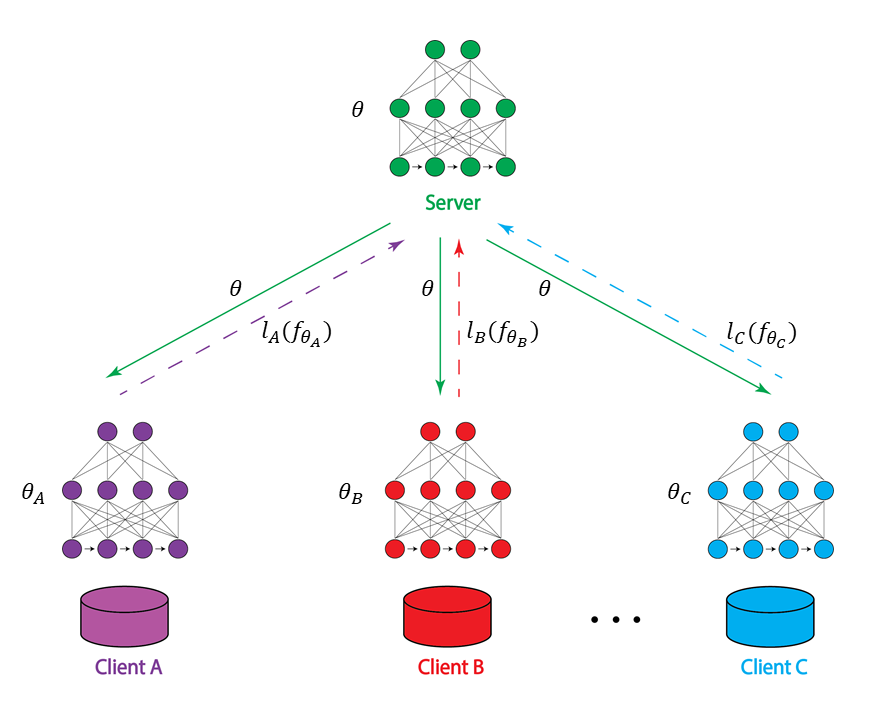
Figure 1: Flowchart of Meta-Federated Learning (MetaFL): After the server distributes the model to all clients, they would finish their local training with their own data. Then, all the losses from the last epoch of their local training would be returned to the server. Finally, the server could update the main model with the integration of the returned losses.

Obviously, for both of algorithms, we need to train various submodels at first and integrate something that is from these submodels to update the main model. For instance, we need to train the clients’ models with the local datasets for Federated Averaging Learning [1], while we need to finish the meta-training of different tasks for MAML [25]. After finishing the integration process, our model could be updated with the integrated result. The only difference between these two algorithms is what we would integrate from different sources. In Federated Averaging algorithm, we directly select model parameters to integrate; while in MAML algorithm, we would integrate the losses from multiple different training tasks. As we stated before, our goal is to design an adaptive federated learning with the basic idea of MAML. Combining these two algorithms, we propose a Meta-Federated Learning (MetaFL) algorithm here, and the key of our algorithm is to return the losses $\mathcal{L}_{k}(f_{\theta})$ from every client $k$ to the server, instead of model parameters $\theta_{k}$. After receiving all the losses, the server would compute the average of them and exploit the integrated loss to update the server model as equation (4). Subsequently, the server would start the new iteration by distributing the new model to all clients and waiting for them to return the new local losses for this iteration. These procedures of MetaFL are visualized in Fig. 1. In other words, compared with the Federated Averaging Learning algorithm, the difference is that what we return from local clients and try to integrate are losses rather than model parameters now. The specific MetaFL algorithm is depicted in Algorithm 1.

Algorithm 1 Meta-Federated Learning

1:randomly initialize $\theta$

2:for each round t = 1, 2, … do

3:     Sample K training tasks from various clients

4:     for all K clients in parallel do

5:         Evaluate $\nabla_{\theta}\mathcal{L}_{k}(f_{\theta})$

6:         Compute adapted local parameters with gradient descent: $\theta_{k}=\theta-\alpha\nabla_{\theta}\mathcal{L}_{k}(f_{\theta})$      

7:     end for

8:     clients return all losses $\mathcal{L}_{k}(f_{\theta_{k}})$ to the server

9:     update the server model with the losses from all clients: $\theta\leftarrow\theta-\beta\nabla_{\theta}\sum_{k=1}^{K}\frac{1}{K}\mathcal{L}_{k}(f_{\theta_{k}})$

10:end for

II-B Partial Meta-Federated Learning (PMFL)

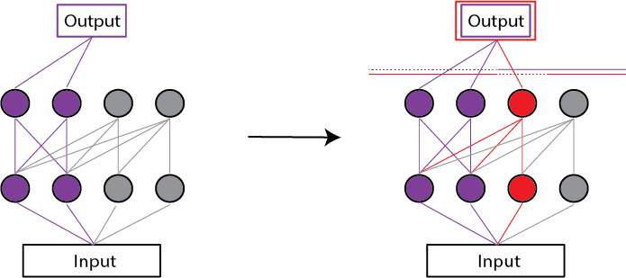
Figure 2: Continual Learning: A simple example of continual learning shows its sparsification scheme.

Transfer learning which focuses on multi-task learning and model generalization is an ideal and perfect utensil to further improve our algorithm. In particular, continual learning, a specific mechanism of transfer learning, could leverage a pre-trained model to train a new task beyond what has been previously trained [40, 41]. Owing to the characteristic of over-parametrization for neural networks, continual learning proposed a sparsification scheme that we just use some active nodes to train the specific task with graceful forgetting. In this case, our model would not suffer any catastrophic forgetting issue. Fig. 2 shows a simple example for continual learning. The subsequent tasks would use the unused weights to learn features since the sparsification scheme allows the current task to train models with only a subset of neurons.

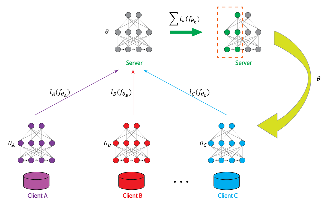
Figure 3: Flowchart of Partial Meta-Federated Learning (PMFL): Similar to MetaFL, the server distributes the main model to all clients, then the clients would train with the local datasets for a few epochs. Then, all the losses from the last epoch of their local training would be returned to the server. After all the losses are delivered to the server, the server would freeze one half of the main model and update the other half with the average loss which is computed with the returned losses from all clients.

Hopefully, by combining our algorithm with this creative scheme, the performance of our model would be promoted positively. In accordance with this thought, we further modify our algorithm and finally propose a Partial Meta-Federated Learning (PMFL) algorithm. Similar to continual learning, we take advantage of the over-parametrization of neural networks by using an activation based neural pruning sparsification scheme to train models which only use a fraction of their width. The explicit steps are included in Fig. 3. Let N denote the total number of nodes in our neural network. Specifically, denoting the first half of our main model parameters $\theta$ with $\theta[:\frac{N}{2}]$ and the second half with $\theta[\frac{N}{2}:]$, our PMFL algorithm would select $\theta[:\frac{N}{2}]$ to update when training with the integrated loss $\sum_{k=1}^{K}\frac{1}{K}\mathcal{L}_{k}(f_{\theta_{k}})$ from all clients, and keep the other half of $\theta[\frac{N}{2}:]$ freezed and unchangeable. And all the clients just trained as normal, which would update all model parameters $\theta_{k}$. By this, the server model has the ability to learn the common features from all various training tasks, and all the clients model could keep their own features. Also, there would be some inactive nodes for our main model to learn future tasks. The steps of the full PMFL algorithm are outlined in Algorithm 2.

Algorithm 2 Partial Meta-Federated Learning

1:randomly initialize $\theta,\theta_{1},\theta_{2},...,\theta_{K}$ $\triangleright$ $\theta$ indicates the server model, and $\theta_{1},\theta_{2},...,\theta_{K}$ indicate K client models

2:for each round t = 1, 2, … do

3:     Sample K training tasks from various clients

4:     for all K clients in parallel do $\triangleright$ each client could update locally in multiple epochs

5:         send the first half of the server model parameters to the client model: $\theta_{k}\leftarrow\theta[:\frac{N}{2}]$

6:         Evaluate $\nabla_{\theta_{k}}\mathcal{L}_{k}(f_{\theta_{k}})$

7:         Compute adapted local parameters with gradient descent: $\theta_{k}\leftarrow\theta_{k}-\alpha\nabla_{\theta_{k}}\mathcal{L}_{k}(f_{\theta_{k}})$      

8:     end for

9:     clients return all losses $\mathcal{L}_{k}(f_{\theta_{k}})$ to the server

10:     freeze the second half of the server model $\theta[\frac{N}{2}:]$

11:     server update with gradient descent: $\theta\leftarrow\theta-\beta\nabla_{\theta}\sum_{k=1}^{K}\frac{1}{K}\mathcal{L}_{k}(f_{\theta_{k}})$ $\triangleright$ update the server model

12:end for

II-C Evaluation

Divergent from the setting of federated learning, for both of our MetaFL and PMFL algorithms, we arrange that the last client which possesses its own dataset is the server for our scheme while the server for federated learning doesn’t include any data and only works for integrating and updating the model. Similar to MAML, after we got the pre-trained model with data from all clients by MetaFL or PMFL algorithm, we would continue to train the model with part of the dataset from this server and test the final model with the other part. Thus, the paramount point for the evaluation procedure is that we would test our trained model with data from the server while training data consists of the datasets from all different clients. It’s because of this arrangement for the server that we are able to train our model directly with the server’s own data regardless of the data of clients. Besides the traditional federated learning algorithm, training directly without any pretraining process also could be compared with our proposed MetaFL and PMFL algorithm. Totally, there are four schemes to be compared.

In order to assess model performance, we need to evaluate our algorithm with different metrics. The model attempts to predict whether patients have certain diseases or not. The outcomes generated from our model are the probabilities for the patients to have this disease. We select thresholds to decide whether the result is positive or otherwise negative for each prediction, where positive means confirmed case. For example, if the output for one sample is 0.48 and we set threshold to be 0.4, then this sample would be a confirmed case. However, if we set threshold to be 0.5, this sample would be a negative case. After comparing our predictions with the true labels, all results would be split into four classes, which are true positive(TP), false positive(FP), true negative(TN), and false negative(FN). After we know how many there are for each class, we could easily derive some crucial metrics, such as recall(TPR) by equation (5), precision by equation (6), FPR by equation (7), and $F_{1}$ score by equation (8).

$$recall(TPR)=\frac{TP}{TP+FN}$$ (5)

$$precision=\frac{TP}{TP+FP}$$ (6)

$$FPR=\frac{FP}{TN+FP}$$ (7)

$$F_{1}=\frac{2}{recall^{-1}+precision^{-1}}$$ (8)

By choosing different thresholds, it’s evident that we could get different number of positive and negative predictions, which would result in different precision, recall and so on. The ROC curve was produced by plotting the true positive rate (TPR or recall) and the false positive rate (FPR or 1-specificity) at thresholds ranging from 0 to 1, while Precision-Recall Curve is based on different precision and recall values. And, ROC AUC which we evaluate is actually the area under the ROC curve. In Fig. 4, we show one example of ROC curve. As you can see, we would get different FPR and TPR with different thresholds even though it doesn’t influence the ROC AUC. Because the precision or other scores will be different if we select different thresholds, unlike ROC AUC, we couldn’t directly exploit these scores to make numeric comparisons and conclude which algorithm is the best. Notwithstanding, the Youden index, the sum of sensitivity and specificity minus one, is an index used for setting optimal thresholds on medical tests, which could provide the best tradeoff between sensitivity and specificity.

$$J=TPR-FPR$$ (9)

where we denote Youden index with $J$.

Therefore, by selecting the threshold to maximize the Youden index as equation (9), we would obtain the optimum cut-off point when our diagnostic test with the metrics, like Precision, Recall, and $F_{1}$ score, gives a numeric rather than a dichotomous result.

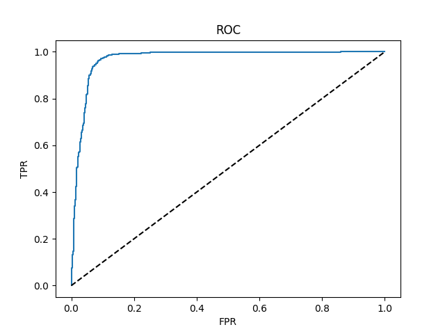
Figure 4: ROC: ROC Curve which results from different thresholds. The ROC curve was produced by plotting the TPR and the FPR.

III Results

III-A MIMIC-CXR v2.0.0

III-A1 Dataset

The MIMIC Chest X-ray (MIMIC-CXR) Database v2.0.0 is a large publicly available dataset of chest radiographs in DICOM format with free-text radiology reports and structured labels derived from these reports. To be specific, the dataset contains 377,110 JPG format images and structured labels derived from the 227,827 free-text radiology reports associated with these images [42, 43, 44, 45]. Despite that we don’t need the image data, a large number of text reports and structured labels could work perfectly for our purpose.

In our experiment, we would mainly use two files from MIMIC-CXR v2.0.0:

• mimic-cxr-reports.tar.gz: a compressed file which include a set of 10 folders, and each folder includes around 6500 sub-folders which are named according to the patient identifier, and contain all the patient’s text reports which are named according to the study identifier.

• mimic-cxr-2.0.0-chexpert.csv.gz: a compressed file listing all studies with labels generated by the CheXpert labeler. The patient identifier and study identifier are also included to match the text reports. Notice that there are several labels unrelated with any disease, like Support Devices and No Findings which we don’t consider in our experiment.

To confirm the extraordinary performance of our proposed algorithm for heterogeneous training tasks, we split the entire dataset into multiple subsets which include different labels to represent different clients. For MIMIC-CXR v2.0.0 dataset, the basic model for all clients and the server would use the text reports of patients from mimic-cxr-reports.tar.gz as input data to classify whether these patients have certain diseases, so the labels for different clients are corresponding to different columns from mimic-cxr-2.0.0-chexpert.csv.gz, and each column of this file includes the information for a single kind of disease. Specifically, we take only 8 kinds of diseases, which are relevant with lung, such as Pneumonia, Lung Lesion, Pneumothorax and so on, into consideration and generate our 8 heterogeneous training tasks. Not only would the selection of similar diseases intuitively make it more sense when testing federated learning and meta-learning algorithm, but it closely resembles the real case scenario of federated learning and meta-learning. In addition, we treat 1 as positive label, otherwise, we would treat it as negative label.

TABLE I: The number of samples for each client and its label. All datasets for clients come from MIMIC-CXR v2.0.0.

client	label	number of samples
1	Pleural Other	4022
2	Lung Lesion	12140
3	Pneumothorax	19224
4	Consolidation	17698
5	Pneumonia	23362
6	Atelectasis	58602
7	Pleural Effusion	27080
8	Lung Opacity	18810

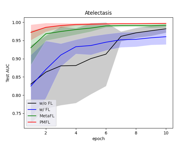
(a) Atelectasis

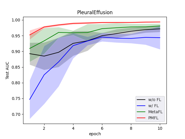
(b) Pleural Effusion

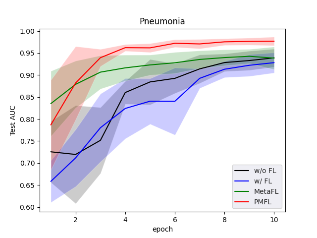
(c) Pneumonia

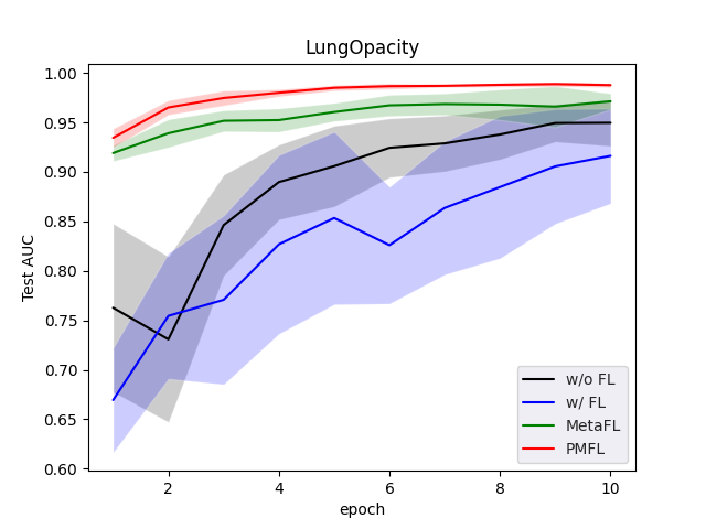
(d) Lung Opacity

Figure 5: Results of MIMIC-CXR v2.0.0 dataset: Plot of average AUC score of our PMFL algorithm, against without FL, original FL, MetaFL when choosing Atelectasis, Consolidation, Pneumonia or Lung Opacity as test task. The lines in this figure show the average AUC of 5 experiments while the thickness of the lines shows the standard deviation for each case.

For the rest, we extract 8 silo datasets from the original dataset by making sure:

• the 1:1 ratio of positive samples and negative samples for each silo.

• first extract data from the class which includes more samples to generate 8 different datasets with similar size in case some clients dominate the learning process. For instance, from the table I, we first select samples of Pleural Other because this class includes the least samples.

Finally, we got 8 different datasets and the size of all datasets could be found in table I. After that, we shuffle all silos to simulate 8 different clients of federated learning or our two algorithms. Importantly, any silo doesn’t overlap with any other silos after splitting the original dataset. It means that each file could only appear in one silo. During the experiment, we would choose one silo as target task, and randomly select any other 5 silos as training tasks to pretrain our model for traditional federated learning, MetaFL and PMFL. For all clients, 90% of the data would be used for training while 10% would be used for testing.

III-A2 Model and performance

Because of the structure of our model, we could separately set different hyper-parameters for the clients’ models and the server model. Clients’ models are responsible for the local training, while the updating process in the server would result in the changes of our main model.

To be specific, because our input data is text, our client model is based on LSTM, and it includes one embedding layer(embedding dimension of 128), one bidirectional LSTM (32 hidden nodes) and one linear layer with one output node. The binary loss function trained with Adam optimizer is adopted to evaluate the result. We settle on the meta learning rate of $10^{-3}$ and set batch size to be varied with respect to the size of local dataset in order to make sure that the number of batches for different clients would be identical, and the number of epochs is $10$ . For our server model, we select 5 clients to train, and the learning rate is $10^{-2}$.

TABLE II: Compare the AUC of ROC, Precision, Recall and F1 score for four different training cases when treat different diseases as target test task. Notice that Precision, Recall and F1 score are obtained with the thresholds which maximize Youden’s Index.

Test task	Algorithm	ROC AUC	Precision	Recall	F1 score
Atelectasis	w/o FL	$0.9920\pm 0.0027$	$0.9709\pm 0.0127$	$0.9872\pm 0.0036$	$0.9789\pm 0.0054$
	FL	$0.9857\pm 0.0097$	$0.9578\pm 0.0219$	$0.9756\pm 0.0107$	$0.9666\pm 0.0159$
	MetaFL	$0.9923\pm 0.0028$	$0.9661\pm 0.0124$	$0.9845\pm 0.0067$	$0.9752\pm 0.0083$
	PMFL	$0.9971\pm 0.0005$	$0.9863\pm 0.0015$	$0.9899\pm 0.0015$	$0.9881\pm 0.0005$
Consolidation	w/o FL	$0.9475\pm 0.0347$	$0.9268\pm 0.0270$	$0.9087\pm 0.0832$	$0.9160\pm 0.0523$
	FL	$0.9475\pm 0.0408$	$0.9148\pm 0.0631$	$0.9284\pm 0.0351$	$0.9204\pm 0.0415$
	MetaFL	$0.9690\pm 0.0208$	$0.9593\pm 0.0242$	$0.9148\pm 0.0757$	$0.9343\pm 0.0398$
	PMFL	$0.9900\pm 0.0041$	$0.9635\pm 0.0096$	$0.9737\pm 0.0074$	$0.9686\pm 0.0084$
Lung Lesion	w/o FL	$0.8733\pm 0.1054$	$0.8621\pm 0.1125$	$0.8083\pm 0.1193$	$0.8339\pm 0.1146$
	FL	$0.9287\pm 0.0267$	$0.9072\pm 0.0327$	$0.8853\pm 0.0628$	$0.8945\pm 0.0352$
	MetaFL	$0.9713\pm 0.0171$	$0.9372\pm 0.0249$	$0.9570\pm 0.0225$	$0.9469\pm 0.0230$
	PMFL	$0.9817\pm 0.0036$	$0.9505\pm 0.0078$	$0.9653\pm 0.0051$	$0.9578\pm 0.0052$
Lung Opacity	w/o FL	$0.9041\pm 0.0152$	$0.8426\pm 0.0375$	$0.9154\pm 0.0711$	$0.8745\pm 0.0245$
	FL	$0.8830\pm 0.0356$	$0.8186\pm 0.0511$	$0.9067\pm 0.0495$	$0.8583\pm 0.0293$
	MetaFL	$0.9669\pm 0.0156$	$0.9339\pm 0.0239$	$0.9575\pm 0.0182$	$0.9455\pm 0.0187$
	PMFL	$0.9882\pm 0.0029$	$0.9605\pm 0.0023$	$0.9723\pm 0.0100$	$0.9663\pm 0.0059$
Pleural Effusion	w/o FL	$0.9436\pm 0.0280$	$0.8957\pm 0.0310$	$0.9208\pm 0.0783$	$0.9063\pm 0.0127$
	FL	$0.9428\pm 0.0111$	$0.8832\pm 0.0202$	$0.9480\pm 0.0271$	$0.9142\pm 0.0163$
	MetaFL	$0.9794\pm 0.0057$	$0.9436\pm 0.0178$	$0.9831\pm 0.0076$	$0.9629\pm 0.0124$
	PMFL	$0.9935\pm 0.0015$	$0.9732\pm 0.0086$	$0.9884\pm 0.0051$	$0.9807\pm 0.0044$
Pleural Other	w/o FL	$0.8702\pm 0.0544$	$0.8334\pm 0.0754$	$0.8304\pm 0.0777$	$0.8297\pm 0.0640$
	FL	$0.7166\pm 0.0671$	$0.6665\pm 0.0541$	$0.7471\pm 0.1110$	$0.7003\pm 0.0694$
	MetaFL	$0.9489\pm 0.0554$	$0.9230\pm 0.0941$	$0.9451\pm 0.0374$	$0.9323\pm 0.0643$
	PMFL	$0.9799\pm 0.0036$	$0.9656\pm 0.0109$	$0.9578\pm 0.0239$	$0.9615\pm 0.0125$
Pneumonia	w/o FL	$0.9394\pm 0.0230$	$0.8802\pm 0.0255$	$0.9305\pm 0.0392$	$0.9041\pm 0.0240$
	FL	$0.9089\pm 0.0349$	$0.8392\pm 0.0460$	$0.9375\pm 0.0229$	$0.8849\pm 0.0288$
	MetaFL	$0.9621\pm 0.0191$	$0.9123\pm 0.0139$	$0.9430\pm 0.0396$	$0.9270\pm 0.0238$
	PMFL	$0.9798\pm 0.0084$	$0.9234\pm 0.0082$	$0.9727\pm 0.0067$	$0.9473\pm 0.0039$
Pneumothorax	w/o FL	$0.9725\pm 0.0044$	$0.9519\pm 0.0079$	$0.9543\pm 0.0204$	$0.9529\pm 0.0089$
	FL	$0.9544\pm 0.0129$	$0.9030\pm 0.0223$	$0.9343\pm 0.0277$	$0.9180\pm 0.0172$
	MetaFL	$0.9801\pm 0.0049$	$0.9613\pm 0.0052$	$0.9672\pm 0.0155$	$0.9642\pm 0.0086$
	PMFL	$0.9887\pm 0.0020$	$0.9700\pm 0.0028$	$0.9781\pm 0.0077$	$0.9740\pm 0.0035$

In addition, to test the performance of our algorithm, we need to create a test model, which would load the trained server model to start training, with one client which we don’t use for training before. Actually, this is the last client mentioned in II-C, which would provide the data for the server training and testing. And the hyperparameters are totally identical with the training clients, besides the batch size of $64$. All models were trained on a single NVIDIA 1080 TI GPU.

Just as we stated before, evaluation metrics include not only the AUC of ROC, but also the precision, recall, F1 score when maximizing the Youden index. By selecting different clients to be training tasks or test task, we compare our PMFL algorithm with three cases, which are training directly without any pretraining process, training with the pre-trained model from the original Federated Averaging Learning algorithm, and training with the pre-trained model from the MetaFL algorithm.

In Fig. 5, we show a few results by choosing Atelectasis, Consolidation, Pneumonia and Lung Opacity as test task when evaluated by the AUC of ROC. Three major conclusions are clearly conveyed by the plot. At first, obviously, when training heterogeneous datasets from different clients, our PMFL algorithm consistently outperforms all three other cases by converging to higher AUCs with fewer epochs. Also, even if MetaFL algorithm couldn’t perform as well as our PMFL algorithm, its performance is evidently better than training directly and federated learning. Interestingly, sometimes after the FL pretraining process, the performance would be even worse than training directly. Probably, this is just because of the heterogeneous property of different clients. Apparently, the knowledge from one task would possibly be useless or even malignant for another different task. Table II shows this result more explicitly. Take Pleural Other for example, training directly after 10 epochs achieves a final AUC of $0.8702$, whereas FL only obtained the AUC of $0.7166$ which is worse than training directly, MetaFL could obtain a better AUC of $0.9489$, and PMFL could further improve the AUC to be $0.9799$.

Second, PMFL converged not only faster but also more stable. In Fig. 5, the thickness of the line represents the standard deviation of the AUC in 5 different experiments. The training process of our PMFL algorithm could converge very fast, mostly in less than 4 epochs. In addition, The red line in the image denotes PMFL algorithm and it’s grossly thinner than the other three lines, especially after training a few epochs. In table II, similarly, when we selected Pleural Other as test task, the standard deviation of the AUC after training 10 epochs is $0.0544$ for training directly, while it’s $0.0671$ for FL, $0.0554$ for MetaFL, and $0.0036$ for PMFL.

Third, we could easily conclude that the improvement of our algorithm is different for different training tasks and test tasks. For instance, when choosing Lung Lesion as test task, training directly could achieve the AUC of $0.8733$, and the MetaFL algorithm could improve it to be $0.9713$ while the PMFL algorithm could further improve it to be $0.9817$; nevertheless, when keeping the training tasks the same but choosing Pleural Other as test task, training directly obtained the AUC of $0.8702$, and MetaFL could improve it to be $0.9489$ while PMFL could further improve it to be $0.9799$. Therefore, the improvement for Lung Lesion task is obviously greater. We believe that this is because the five training tasks are more similar to Lung Lesion when compared with Pleural Other. To show this more persuasively, we also try to treat Lung Lesion as test task but selected five different training tasks and we find that the improvements of MetaFL and PMFL also change.

Besides, we also compare the performance of PMFL algorithm with 3 clients and 5 clients. In Fig. 6, the blue line shows the result of 3-clients while the red line denotes 5-clients case and the black line is the result of training directly. At first, we could conclude that the final performance after 10 epochs of training with 3-clients PMFL is extremely similar to the 5-clients PMFL’s. However, apparently, the standard deviation of the blue line is smaller. It means that 3-clients PMFL is more stable than 5-clients PMFL. The results from table III show this more clearly. Both PMFL algorithms perform better than training directly, and their final ROC AUC scores are almost the same while the standard deviation of 3-clients PMFL is $0.0029$ which is slightly smaller than $0.0033$ of 5-clients. And this also makes sense, because when you pretrain the model with more different tasks, the heterogeneous property would make a bigger influence.

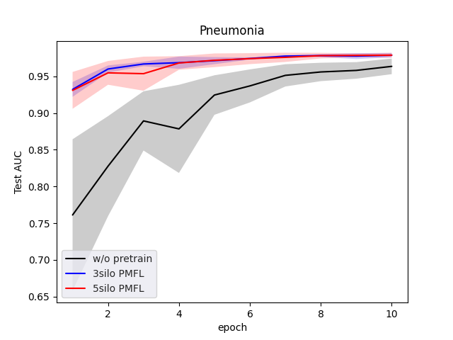
Figure 6: Plot of average AUC score for without pretrain, with 3-clients PMFL, with 5-clients PMFL when choosing Pneumonia as test task. The lines in this figure show the average AUC of 5 experiments while the thickness of the lines shows standard deviation for each case.

TABLE III: Compare ROC AUC for training directly without any pretrain process, PMFL with 3 clients, and PMFL with 5 clients when treat Pneumonia as target test task.

Test task	Algorithm	ROC AUC
Pneumonia	w/o pretrain	$0.9636\pm 0.0106$
	3-clients PMFL	$0.9788\pm 0.0029$
	5-clients PMFL	$0.9789\pm 0.0033$

III-B eICU

III-B1 Dataset

The eICU collaborative Reseach Database, collected through the Philips eICU program, contains highly granular critical care data of 200,859 patients admitted to 208 hospitals from across the United States [46]. For the purpose of our study, we mainly utilized three files:

• admissionDrug.csv.gz: a compressed file which contains details of medications that a patient was taking prior to admission to the ICU. This table includes the patient identifier and admission drug information for this patient such as the drug name, dosage, timeframe during which the drug was administered, the user type and specialty of the clinician entering the data, and the note type where the information was entered.

• patient.csv.gz: a compressed file providing patient demographics and admission and discharge details for hospital and ICU stays.

• admissionDx.csv.gz: a compressed file that includes the patient identifier and the primary diagnosis for admission to the ICU per the APACHE scoring criteria. Entered in the patient note forms.

TABLE IV: The number of samples for each client and its label. All datasets for clients come from eICU.

client	label	number of samples
1	CVA	4483
2	CHF	4495
3	Pneumonia	4280
4	pulmonary	5339
5	Sepsis	5429

With these three files, we could simply obtain the disease labels for each patient from the apacheadmissiondx variable in the patient.csv.gz file. In order to generate the diagnosis text data for each patient, we extract all the drug names for this patient from the admissionDrug.csv.gz file and the diagnosis data from the admissionDx.csv.gz table, and integrated them into a single text file for this patient. Finally, we got 40678 effective patient samples for our research, and 7 different disease labels for each sample. In order to generate the heterogeneous tasks for our experiment, with the same scheme of MIMIC-CXR x2.0.0, we extract 5 silo datasets from the original dataset by making sure:

• the 1:1 ratio of positive samples and negative samples for each silo.

• first select data from the class which includes more samples to generate 5 different datasets with similar size.

Table IV shows the number of samples for each client and its label in detail. After that, we would select three different clients for training tasks to pretrain the traditional federeated learning, MetaFL, and PMFL models, and select another one for test task to evaluate in the server.

III-B2 Model and performance

Similar to the model for MIMIC dataset, a simple LSTM model worked as our meta model. Also, it includes one embedding layer(embedding dimension of 128), one bidirectional LSTM(32 hidden nodes) and one linear layer with one output node. To show the better performance for this dataset, we decrease the batch size to be one half of the MIMIC dataset while all the other hyperparameters the same.

TABLE V: Compare the results of eICU for four different algorithms with the same metrics. In this table, Precision, Recall and F1 score are obtained with the threshold which maximizes Youden’s Index.

Dataset	Algorithm	ROC AUC	Precision	Recall	F1 score
eICU	w/o FL	$0.9218\pm 0.0217$	$0.7296\pm 0.0821$	$0.8733\pm 0.0814$	$0.7877\pm 0.0294$
	FL	$0.8774\pm 0.0524$	$0.7160\pm 0.0662$	$0.7867\pm 0.1035$	$0.7461\pm 0.0672$
	MetaFL	$0.9299\pm 0.0181$	$0.7226\pm 0.0556$	$0.9033\pm 0.0823$	$0.7983\pm 0.0328$
	PMFL	$0.9562\pm 0.0090$	$0.7671\pm 0.0855$	$0.9333\pm 0.0667$	$0.8358\pm 0.0235$

For this dataset, we also compare our PMFL algorithm with training directly, regular federated learning and the MetaFL algorithm with the same metrics. In Fig. 7, this is the result of eICU dataset for evaluating the AUC metric when treated CHF, pneumonia, and pulmonary as the training task labels for clients and treating CVA as the test task label for the server evaluation. At first, obviously, we could find that compared with the regular training, the regular federated learning couldn’t work for heterogeneous datasets but worsen the training performance for our eICU dataset, by comparing the black line with the blue line in the figure. Actually, it performs largely worse for this dataset when compared with MIMIC-CXR v2.0.0 dataset, and I believe that this is because the tasks for all clients are more different. In addition, when comparing the red line with others, our algorithm still outperforms all the other three methods. From the clearer result in table V, we could observe that our PMFL algorithm could improve the AUC of training directly from 0.9218 to 0.9562 after training 10 epochs, which is evidently better than FL and MetaFL algorithm. Also, the standard deviation of our PMFL shows a more competitive result while MetaFL slightly improves the performance of training directly. However, with the regular federated learning pretraining, the result is significantly terrible. Not only does the AUC score decrease to 0.8774, the standard deviation also increases from 0.0217 to 0.0524. Also, for the precision, recall, and F1 score at the threshold when maximizing the Youden’s index, our PMFL algorithm still shows the best result.

By comparing the results of MIMIC-CXR v2.0.0 and eICU datasets, we could find that the performance of regular federated learning would be influenced a lot by the heterogeneous property while the influence is considerably weakened by our proposed algorithms. With the more different training tasks, the regular federated learning would perform worse.

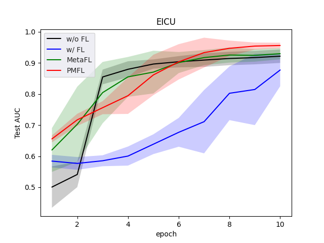
Figure 7: eICU dataset result: Plot of average AUC score of our PMFL algorithm against without FL, with regular FL, with MetaFL when choosing CHF, Pneumonia or pulmonary as training task and select CVA as test task. The lines in this figure show the average AUC of 5 experiments while the thickness of the lines shows standard deviation for each case.

IV Discussion

In this paper, we find that the performance of the normal federated learning would decrease more while our proposed MetaFL and PMFL algorithms perform more stably, when the divergence of tasks from different clients gets bigger. Nevertheless, we believe that there is some limit for our proposed algorithms. And if the divergence between different tasks goes beyond this limit, our algorithms would also perform dreadfully.

Therefore, future research could focus on exploring this limit for our algorithms. To be specific, we could define the distance between different tasks. The bigger distance of two tasks means that these two tasks are more different. It’s overt that how to compute this distance is also a promising future research direction. After we figure out how to compute this distance, we could easily explore the relationship between this distance and the performance of all different algorithms. Also, the limit for our proposed MetaFL and PMFL algorithms could be simply obtained. In addition, if the distance between tasks is extremely small, we believe that the regular federated learning algorithm would also perform very well. Based on this, for different clients, we could quickly judge whether their datasets could be utilized by the regular Federated Learning. Further, we could know the most suitable algorithm for different cases with this distance.

Besides, during our experiments, we try to generate clients with similar sizes. But what if the size is hugely different? Thus, the other viable research direction is to explor the influence of imbalanced datasets. In this case, maybe the training task of the client which includes the most samples would dominate other clients whose datasets are considerably small.

V Conclusion

When the mobile devices, such as smartphones, tablets, and laptops, become more and more popular, a large amount of data could be provided for training. Certainly, by effectively exploiting these data, more robust machine learning models would be easily achieved. While traditional Federated learning, like FedAvg algorithm, has been proved that it’s really helpful for homogeneous training with distributed data, it’s not suitable for heterogeneous training tasks. In order to successfully apply federated learning to heterogeneous datasets, meta-learning, which is able to train an adaptive model, would be a perfect option for us to borrow some ideas. Not only is the structure of meta-learning algorithm really similar to federated learning, but the ability of meta-learning to learn how to learn is absolutely beneficial to heterogeneous training. In this paper, we have confirmed that our new federated learning algorithm(MetaFL), the effective combination of federated learning and meta-learning, significantly outperforms the regular federated learning for heterogeneous tasks. It achieves not only the better ROC AUC or other scores but the faster training speed.

Furthermore, due to the advantage of transfer learning for model generalization, the integration of transfer learning and our algorithm, which is partial meta-federated learning (PMFL), further improve the model performance when compared with the previous one.

Appendix

For the MIMIC-CXR v2.0.0 dataset, there are 8 missing records in the table, which are s58235663.txt in the p11573679 folder, s50798377.txt in the p12632853 folder, s54168089.txt in the p14463099 folder, s53071062.txt in the p15774521 folder, s56724958.txt in the p16175671 folder, s54231141.txt in the p16312859 folder, s53607029.txt in the p17603668 folder, s52035334.txt in the p19349312 folder. Therefore, we just delete these files directly.

References

- [1] H. B. McMahan, E. Moore, D. Ramage, S. Hampson, and B. A. y Arcas, “Communication-efficient learning of deep networks from decentralized data,” 2017.
- [2] J. Konečný, H. B. McMahan, D. Ramage, and P. Richtárik, “Federated optimization: Distributed machine learning for on-device intelligence,” 2016.
- [3] K. Bonawitz, V. Ivanov, B. Kreuter, A. Marcedone, H. B. McMahan, S. Patel, D. Ramage, A. Segal, and K. Seth, “Practical secure aggregation for privacy-preserving machine learning,” in Proceedings of the 2017 ACM SIGSAC Conference on Computer and Communications Security. ACM, Oct. 2017. [Online]. Available: https://doi.org/10.1145/3133956.3133982
- [4] J. Konečný, H. B. McMahan, F. X. Yu, P. Richtárik, A. T. Suresh, and D. Bacon, “Federated learning: Strategies for improving communication efficiency,” 2017.
- [5] F. Chen, M. Luo, Z. Dong, Z. Li, and X. He, “Federated meta-learning with fast convergence and efficient communication,” 2019.
- [6] V. Smith, C.-K. Chiang, M. Sanjabi, and A. Talwalkar, “Federated multi-task learning,” in Proceedings of the 31st International Conference on Neural Information Processing Systems, ser. NIPS’17. Red Hook, NY, USA: Curran Associates Inc., 2017, p. 4427–4437.
- [7] Y. Zhao, M. Li, L. Lai, N. Suda, D. Civin, and V. Chandra, “Federated learning with non-iid data,” 2018.
- [8] R. C. Geyer, T. Klein, and M. Nabi, “Differentially private federated learning: A client level perspective,” 2018.
- [9] Q. Yang, Y. Liu, T. Chen, and Y. Tong, “Federated machine learning: Concept and applications,” vol. 10, no. 2, 2019. [Online]. Available: https://doi.org/10.1145/3298981
- [10] Y. Lin, S. Han, H. Mao, Y. Wang, and W. J. Dally, “Deep gradient compression: Reducing the communication bandwidth for distributed training,” 2020.
- [11] A. Sadilek, L. Liu, D. Nguyen, M. Kamruzzaman, B. Rader, A. Ingerman, S. Mellem, P. Kairouz, E. O. Nsoesie, J. MacFarlane, A. Vullikanti, M. Marathe, P. Eastham, J. S. Brownstein, M. Howell, and J. Hernandez, “Privacy-first health research with federated learning,” medRxiv, 2020. [Online]. Available: https://www.medrxiv.org/content/early/2020/12/24/2020.12.22.20245407
- [12] G. H. Lee and S.-Y. Shin, “Federated learning on clinical benchmark data: Performance assessment,” J Med Internet Res, vol. 22, no. 10, p. e20891, Oct 2020. [Online]. Available: http://www.jmir.org/2020/10/e20891/
- [13] S. Boughorbel, F. Jarray, N. Venugopal, S. Moosa, H. Elhadi, and M. Makhlouf, “Federated uncertainty-aware learning for distributed hospital ehr data,” 2019.
- [14] J. Xu, B. S. Glicksberg, C. Su, P. Walker, J. Bian, and F. Wang, “Federated learning for healthcare informatics,” 2020.
- [15] B. Pfitzner, N. Steckhan, and B. Arnrich, “Federated learning in a medical context: A systematic literature review,” ACM Trans. Internet Technol., vol. 21, no. 2, Jun. 2021. [Online]. Available: https://doi.org/10.1145/3412357
- [16] J. Lee, J. Sun, F. Wang, S. Wang, C.-H. Jun, and X. Jiang, “Privacy-preserving patient similarity learning in a federated environment: Development and analysis,” JMIR Medical Informatics, vol. 6, no. 2, 2018. [Online]. Available: https://par.nsf.gov/biblio/10064144
- [17] L. Huang and D. Liu, “Patient clustering improves efficiency of federated machine learning to predict mortality and hospital stay time using distributed electronic medical records,” 2019.
- [18] D. Liu, D. Dligach, and T. Miller, “Two-stage federated phenotyping and patient representation learning,” 2019.
- [19] D. Liu, T. Miller, R. Sayeed, and K. D. Mandl, “Fadl:federated-autonomous deep learning for distributed electronic health record,” 2018.
- [20] T. S. Brisimi, R. Chen, T. Mela, A. Olshevsky, I. C. Paschalidis, and W. Shi, “Federated learning of predictive models from federated electronic health records,” International Journal of Medical Informatics, vol. 112, pp. 59–67, 2018. [Online]. Available: https://www.sciencedirect.com/science/article/pii/S138650561830008X
- [21] A. Rajeswaran, C. Finn, S. Kakade, and S. Levine, “Meta-learning with implicit gradients,” in NeurIPS, 2019.
- [22] J. Schmidhuber, “Evolutionary principles in self-referential learning. on learning now to learn: The meta-meta-meta…-hook,” Diploma Thesis, Technische Universitat Munchen, Germany, 1987. [Online]. Available: http://www.idsia.ch/~juergen/diploma.html
- [23] S. Bengio, Y. Bengio, J. Cloutier, and J. Gecsei, “On the optimization of a synaptic learning rule,” 1997.
- [24] C. Finn and S. Levine, “Meta-learning and universality: Deep representations and gradient descent can approximate any learning algorithm,” 2018.
- [25] C. Finn, P. Abbeel, and S. Levine, “Model-agnostic meta-learning for fast adaptation of deep networks,” 2017.
- [26] T. Hospedales, A. Antoniou, P. Micaelli, and A. Storkey, “Meta-learning in neural networks: A survey,” 2020.
- [27] J. Vanschoren, “Meta-learning: A survey,” 10 2018.
- [28] O. Vinyals, C. Blundell, T. Lillicrap, K. Kavukcuoglu, and D. Wierstra, “Matching networks for one shot learning,” in Proceedings of the 30th International Conference on Neural Information Processing Systems, ser. NIPS’16. Curran Associates Inc., 2016, p. 3637–3645.
- [29] A. Santoro, S. Bartunov, M. Botvinick, D. Wierstra, and T. Lillicrap, “Meta-learning with memory-augmented neural networks,” in Proceedings of the 33rd International Conference on International Conference on Machine Learning - Volume 48, ser. ICML’16. JMLR.org, 2016, p. 1842–1850.
- [30] A. Graves, G. Wayne, and I. Danihelka, “Neural turing machines,” 2014.
- [31] S. Ravi and H. Larochelle, “Optimization as a model for few-shot learning,” in ICLR, 2017.
- [32] T. Munkhdalai and H. Yu, “Meta networks,” in Proceedings of the 34th International Conference on Machine Learning, ser. Proceedings of Machine Learning Research, D. Precup and Y. W. Teh, Eds., vol. 70. PMLR, 06–11 Aug 2017, pp. 2554–2563. [Online]. Available: http://proceedings.mlr.press/v70/munkhdalai17a.html
- [33] A. Nichol, J. Achiam, and J. Schulman, “On first-order meta-learning algorithms,” 2018.
- [34] P. Zhang, J. Li, Y. Wang, and J. Pan, “Domain adaptation for medical image segmentation: A meta-learning method,” Journal of Imaging, vol. 7, no. 2, 2021. [Online]. Available: https://www.mdpi.com/2313-433X/7/2/31
- [35] H. Park, G. M. Lee, S. Kim, G. H. Ryu, A. Jeong, S. H. Park, and M. Sagong, “A meta-learning approach for medical image registration,” 2021.
- [36] S. Hu, J. M. Tomczak, and M. Welling, “Meta-learning for medical image classification,” in 1st Conference on Medical Imaging with Deep Learning (MIDL 2018), 2018.
- [37] K. Mahajan, M. Sharma, and L. Vig, “Meta-dermdiagnosis: Few-shot skin disease identification using meta-learning,” in 2020 IEEE/CVF Conference on Computer Vision and Pattern Recognition Workshops (CVPRW), 2020, pp. 3142–3151.
- [38] R. Khadga, D. Jha, S. Ali, S. Hicks, V. Thambawita, M. A. Riegler, and P. Halvorsen, “Few-shot segmentation of medical images based on meta-learning with implicit gradients,” 2021.
- [39] Y. Chen, C. Guan, Z. Wei, X. Wang, and W. Zhu, “Metadelta: A meta-learning system for few-shot image classification,” 2021.
- [40] J. Yoon, E. Yang, J. Lee, and S. J. Hwang, “Lifelong learning with dynamically expandable networks,” arXiv preprint arXiv:1708.01547, 2017.
- [41] S. Golkar, M. Kagan, and K. Cho, “Continual learning via neural pruning,” arXiv preprint arXiv:1903.04476, 2019.
- [42] A. Johnson, T. Pollard, R. Mark, S. Berkowitz, and S. Horng, “Mimic-cxr database,” PhysioNet https://doi. org/10.13026/C2JT1Q, 2019.
- [43] A. E. Johnson, T. J. Pollard, N. R. Greenbaum, M. P. Lungren, C.-y. Deng, Y. Peng, Z. Lu, R. G. Mark, S. J. Berkowitz, and S. Horng, “Mimic-cxr-jpg, a large publicly available database of labeled chest radiographs,” arXiv preprint arXiv:1901.07042, 2019.
- [44] A. L. Goldberger, L. A. Amaral, L. Glass, J. M. Hausdorff, P. C. Ivanov, R. G. Mark, J. E. Mietus, G. B. Moody, C.-K. Peng, and H. E. Stanley, “Physiobank, physiotoolkit, and physionet: components of a new research resource for complex physiologic signals,” circulation, vol. 101, no. 23, pp. e215–e220, 2000.
- [45] A. Johnson, M. Lungren, Y. Peng, Z. Lu, R. Mark, S. Berkowitz, and S. Horng, “Mimic-cxr-jpg-chest radiographs with structured labels.”
- [46] T. J. Pollard, A. E. Johnson, J. D. Raffa, L. A. Celi, R. G. Mark, and O. Badawi, “The eicu collaborative research database, a freely available multi-center database for critical care research,” Scientific data, vol. 5, no. 1, pp. 1–13, 2018.