Robustness Certificates for Implicit Neural Networks:
A Mixed Monotone Contractive Approach

Abstract

Implicit neural networks are a general class of learning models that replace the layers in traditional feedforward models with implicit algebraic equations. Compared to traditional learning models, implicit networks offer competitive performance and reduced memory consumption. However, they can remain brittle with respect to input adversarial perturbations.

This paper proposes a theoretical and computational framework for robustness verification of implicit neural networks; our framework blends together mixed monotone systems theory and contraction theory. First, given an implicit neural network, we introduce a related embedded network and show that, given an $\ell_{\infty}$-norm box constraint on the input, the embedded network provides an $\ell_{\infty}$-norm box overapproximation for the output of the given network. Second, using $\ell_{\infty}$-matrix measures, we propose sufficient conditions for well-posedness of both the original and embedded system and design an iterative algorithm to compute the $\ell_{\infty}$-norm box robustness margins for reachability and classification problems. Third, of independent value, we propose a novel relative classifier variable that leads to tighter bounds on the certified adversarial robustness in classification problems. Finally, we perform numerical simulations on a Non-Euclidean Monotone Operator Network (NEMON) trained on the MNIST dataset. In these simulations, we compare the accuracy and run time of our mixed monotone contractive approach with the existing robustness verification approaches in the literature for estimating the certified adversarial robustness.

1 Introduction

Neural networks are increasingly being deployed in real-world applications, including natural language processing, computer vision, and self-driving vehicles. However, they are notoriously vulnerable to adversarial attacks; slight perturbations in the input can lead to large deviations in the output (Szegedy et al., 2014). Understanding this input sensitivity is essential in safety-critical applications, since the consequences of adversarial perturbations can be disastrous. Several different strategies have been proposed in the literature to design neural networks that are robust with respect to adversarial perturbations (Goodfellow et al., 2015; Papernot et al., 2016). Unfortunately, many of these approaches are based on robustness with respect to specific attacks and they do not provide formal robustness guarantees (Madry et al., 2018; Carlini and Wagner, 2017). Recently, there has been a large interest in providing provable robustness guarantees for neural networks. Most existing approaches focus on either the $\ell_{2}$-norm or $\ell_{\infty}$-norm robustness measures. For neural networks with high-dimensional inputs and subject to dense perturbations, the $\ell_{2}$-norm robustness measures are known to provide overly conservative estimates of robustness and are less informative than their $\ell_{\infty}$-norm counterparts. Rigorous verification methods generally fall into four different categories (i) Lipschitz bound methods (Fazlyab et al., 2019; Virmaux and Scaman, 2018; Combettes and Pesquet, 2020), (ii) interval bound methods (Mirman et al., 2018; Gowal et al., 2018; Zhang et al., 2020), (iii) optimization-based methods (Wong and Kolter, 2018; Zhang et al., 2018), and (iv) probabilistic methods (Cohen et al., 2019; Li et al., 2019). However, these methods suffer from several limitations. Regarding the Lipschitz bound approach, the proposed methods are either too conservative (Szegedy et al., 2014) or not scalable to large-scale problems (Virmaux and Scaman, 2018; Combettes and Pesquet, 2020). Similar concerns apply to interval-bound propagation methods and optimization-based methods. Finally, probabilistic approaches provide some guarantees for $\ell_{1}$ and $\ell_{2}$-norm robustness but there are theoretical limitations in their applicability for certifying $\ell_{\infty}$-robustness (Blum et al., 2020).

In this paper we study the robustness properties of implicit neural networks, a recently proposed class of learning models with strong scalability properties. Implicit neural networks replace the notion of layer from traditional neural networks with an implicit fixed-point equation (Bai et al., 2019; El Ghaoui et al., 2021). They can be considered as infinite-depth weight-tied neural networks where recursive function evaluation is performed via solving a single implicit algebraic equation. The implicit framework generalizes many classical neural networks including feedforward, convolutional, and residual networks (El Ghaoui et al., 2021). Implicit neural networks are inspired by biological systems and, compared to traditional neural networks, they offer competitive accuracy and reduced memory consumption (Bai et al., 2019). Additionally, preliminary empirical evidence indicates that appropriately-trained implicit neural networks are more robust than traditional feedforward models (Pabbaraju et al., 2021); however this phenomenon is not yet well understood and open questions remain regarding the stability and robustness of implicit models.

We propose a rigorous computationally efficient certification method for implicit neural network robustness. We note that many of the classical robustness analysis tools for traditional neural networks are either not applicable to implicit neural networks or will lead to conservative results. Our novel approach is derived from mixed monotone systems theory and contraction theory. Unlike the robustness verification approaches based on estimates of Lipschitz constants, our framework takes into account how the $\ell_{\infty}$-error bounds propagate through the network and is scalable with the size of the network.

Related works

Implicit learning models.

Implicit neural networks have been proposed as a generalization of feedforward neural networks (Bai et al., 2019; El Ghaoui et al., 2021). In (Kag et al., 2020), it is demonstrated that implicit models generally do not suffer from vanishing nor exploding gradients. One of the main challenges in studying implicit neural networks is their well-posedness, i.e., existence and uniqueness of solutions for their fixed-point equation. (El Ghaoui et al., 2021) proposes a sufficient spectral condition for convergence of the Picard iterations associated with the fixed-point equation. In (Winston and Kolter, 2020; Revay et al., 2020), using monotone operator theory, a suitable parametrization of the weight matrix is proposed which guarantees the stable convergence of suitable fixed-point iterations. Our previous work (Jafarpour et al., 2021) proposes non-Euclidean contraction theory to design implicit neural networks and study their well-posedness, stability, and robustness with respect to the $\ell_{\infty}$-norm; the general theory is developed in (Davydov et al., 2021) and a short tutorial is given in (Bullo et al., 2021).

Robustness of neural networks.

Starting with (Szegedy et al., 2014), there has been a large body of work in machine learning to understand adversarial examples (Athalye et al., 2018). Several examples for certified robustness training and analysis include (Wong and Kolter, 2018; Zhang et al., 2018; Gowal et al., 2018; Zhang et al., 2020; Mirman et al., 2018; Cohen et al., 2019). Regarding implicit neural networks, there are far fewer works on their robustness guarantees. In (El Ghaoui et al., 2021) a sensitivity-based robustness analysis for implicit neural network is proposed. Approximation of the Lipschitz constants of deep equilibrium networks has been studied in (Pabbaraju et al., 2021; Revay et al., 2020). Recently, the ellipsoid methods based on semi-definite programming (Chen et al., 2021) and the interval-bound propagation method (Anonymous, 2022) have been proposed for robustness certification of deep equilibrium networks.

Mixed monotone system theory.

Mixed monotone systems theory (Enciso et al., 2006; Angeli et al., 2014; Coogan and Arcak, 2015; Coogan, 2020) provides a generalization of classical monotone systems theory (Smith, 1995; Farina and Rinaldi, 2000; Angeli and Sontag, 2003), applicable to all dynamical systems bearing a locally Lipschitz continuous vector field (Yang and Ozay, 2019; Abate et al., 2021). A dynamical system is mixed monotone when there exists a related decomposition function that separates the system’s vector field or update map into increasing and decreasing components. Such a decomposition then facilitates robustness analysis for the initial mixed monotone system and specifically enables, e.g., the efficient computation of robust reachable sets and invariant sets (Abate and Coogan, 2020).

Contributions

Based on mixed monotone system theory, this paper proposes a theoretical and computational framework to study the robustness of implicit neural networks. Given an implicit neural network, we introduce an associated embedded network with twice as many inputs and outputs as the original system. This embedded implicit network takes an $\ell_{\infty}$-norm box as its input and generates an $\ell_{\infty}$-norm box as its output. Then, we study the connection between the well-posedness of the embedded network and the robustness of the original implicit network. Our main theoretical contribution is as follows: if the $\ell_{\infty}$-matrix measure of the original network’s weight matrix is less than one, then (i) the implicit neural network has a unique fixed-point, (ii) the embedded network has a unique fixed-point which can be computed using a suitable average-iteration, and (iii) for a given $\ell_{\infty}$-norm box constraint on the input of the implicit neural network, the output of the embedded implicit neural network is an $\ell_{\infty}$-norm box overapproximation of output the original implicit network. In particular, result (iii) above shows how bounds on the network output are obtained directly from bounds on the network input, allowing for efficient reachability analysis for implicit neural networks. However, the output bounds obtained using this approach can lead to conservative robustness estimates in classifications. As a practical contribution, we propose a new classifier variable, again based upon mixed monotone theory, that leads to sharper robustness estimates in classification. In order to evaluate the robustness guarantees of implicit neural networks, we empirically examine their certified adversarial robustness. We then use (i) estimates of Lipschitz bounds, (ii) the interval bound propagation method, and (iii) our mixed monotone contractive approach to provide lower bounds on certified adversarial robustness. Finally, we compare the certified adversarial robustness of the three approaches mentioned above on a pre-trained implicit neural network. Our simulation results show that the mixed monotone contractive approach significantly outperforms the other two methods.

2 Mathematical preliminaries

Vectors and matrices.

Given a matrix $B\in\mathbb{R}^{n\times m}$, we denote the non-negative part of $B$ by $[B]^{+}=\max(B,0)$ and the nonpositive part of $B$ by $[B]^{-}=\min(B,0)$. The Metzler part and the non-Metzler part of square matrix $A\in^{n\times n}$ are denoted by $\lceil A\rceil^{\mathrm{Mzl}}\in^{n\times n}$ and $\lfloor A\rfloor^{\mathrm{Mzl}}\in^{n\times n}$, respectively, where

$$(\lceil A\rceil^{\mathrm{Mzl}})_{ij} =\begin{cases}A_{ij}&A_{ij}\geq 0\;\mbox{or}\;i=j\\ 0&\mbox{otherwise,}\end{cases}\qquad\lfloor A\rfloor^{\mathrm{Mzl}}=A-\lceil A\rceil^{\mathrm{Mzl}}.$$

We note that, for every square matrix $A\in^{n\times n}$, $\lceil A\rceil^{\mathrm{Mzl}}$ is a Metzler matrix and $\lfloor A\rfloor^{\mathrm{Mzl}}$ is a non-positive matrix with zero diagonal elements. For matrices $C\in^{n\times m}$ and $D\in^{p\times q}$, the Kronecker product of $C$ and $D$ is denoted by $C\otimes D$.

Matrix measures and weak pairings.

For every $\eta\in^{n}_{>0}$, we define the diagonal matrix $[\eta]\in^{n\times n}$ by $[\eta]_{ii}=\eta_{i}$, for every $i\in\{1,\ldots,n\}$. For $\eta\in^{n}_{>0}$, the diagonally weighted $\ell_{\infty}$-norm is defined by $\|x\|_{\infty,[\eta]^{-1}}=\max_{i}|x_{i}|/\eta_{i}$, the diagonally weighted $\ell_{\infty}$-matrix measure is defined by $\mu_{\infty,[\eta]^{-1}}(A)=\max_{i\in\{1,\dots,n\}}A_{ii}+\sum_{j\neq i}\frac{\eta_{j}}{\eta_{i}}|A_{ij}|$. We note that, for every $\eta\in^{n}_{>0}$ and every square matrix $A\in^{n\times n}$, we have

$$\mu_{\infty,[\eta]^{-1}}(A)=\mu_{\infty,I_{2}\otimes[\eta]^{-1}}\left(\begin{bmatrix}\lceil A\rceil^{\mathrm{Mzl}}&\lfloor A\rfloor^{\mathrm{Mzl}}\\ \lfloor A\rfloor^{\mathrm{Mzl}}&\lceil A\rceil^{\mathrm{Mzl}}\end{bmatrix}\right).$$ (1)

From (Davydov et al., 2021, Table III), we define the weak pairing $\left\llbracket{\cdot},{\cdot}\right\rrbracket:^{n}\times^{n}\rightarrow$ associated to the norm $\|\cdot\|_{\infty,[\eta]^{-1}}$ as follows:

$$\left\llbracket{x},{y}\right\rrbracket=\max_{i\in I_{\infty}([\eta]^{-1}y)}\eta_{i}^{-2}y_{i}x_{i},$$

where $I_{\infty}(x)=\{i\in\{1,\dots,n\}\;|\;|x_{i}|=\|x\|_{\infty}\}$.

Lipschitz and one-sided Lipschitz constants.

Let $\mathsf{F}:^{n}\times^{m}\to^{n}$ be a locally Lipschitz map in the first argument. For every $u\in^{m}$ and every $\alpha\in(0,1]$, we define the $\alpha$-average map $\mathsf{F}_{\alpha}:^{n}\times^{m}\to^{n}$ by $\mathsf{F}_{\alpha}=(1-\alpha)\mathsf{I}+\alpha\mathsf{F}$, where $\mathsf{I}$ is the identity map on ⁿ. Given a positive vector $\eta\in^{n}_{>0}$, $\mathsf{F}(x,u)$ is Lipschitz in $x$ with respect to the norm $\|\cdot\|_{\infty,[\eta]^{-1}}$ with constant $\operatorname{Lip}^{x}_{\infty,[\eta]^{-1}}(\mathsf{F})\in_{\geq 0}$ if, for every $x_{1},x_{2}\in^{n}$ and every $u\in^{m}$,

$$\|\mathsf{F}(x_{1},u)-\mathsf{F}(x_{2},u)\|_{\infty,[\eta]^{-1}}\leq\operatorname{Lip}^{x}_{\infty,[\eta]^{-1}}(\mathsf{F})\|x_{1}-x_{2}\|_{\infty,[\eta]^{-1}},$$

For every $u\in^{m}$, we define the set $\Omega_{u}=\{x\in^{n}\;|\;\frac{\partial\mathsf{F}(x,u)}{\partial x}\;\;\mbox{exists}\}$. By Rademacher’s theorem, the set ${}^{n}/\Omega_{u}$ is a measure zero set, for every $u\in^{m}$. The map $\mathsf{F}(x,u)$ is one-sided Lipschitz in $x$ with respect to the norm $\|\cdot\|_{\infty,[\eta]^{-1}}$ with constant $\operatorname{osL}^{x}_{\infty,[\eta]^{-1}}(\mathsf{F})\in$ if, for every $x_{1},x_{2}\in^{n}$ and every $u\in^{m}$,

$$\left\llbracket{\mathsf{F}(x_{1},u)-\mathsf{F}(x_{2},u)},{x_{1}-x_{2}}\right\rrbracket\leq\operatorname{osL}^{x}_{\infty,[\eta]^{-1}}(\mathsf{F})\|x_{1}-x_{2}\|^{2}_{\infty,[\eta]^{-1}},$$

and we define $\operatorname{diagL}(\mathsf{F})\in[-\operatorname{Lip}^{x}_{\infty,[\eta]^{-1}}(\mathsf{F}),\operatorname{Lip}^{x}_{\infty,[\eta]^{-1}}(\mathsf{F})]$ by

$$\operatorname{diagL}(\mathsf{F})=\min_{i\in\{1,\ldots,n\}}\inf_{u\in^{m}}\inf_{x\in\Omega_{u}}D_{x}\mathsf{F}_{ii}(x,u),$$

Mixed monotone mappings.

Given a map $\mathsf{F}:^{n}\times^{m}\to^{n}$ and a Lipschitz function $d:^{2n}\times^{2m}\to^{n}$, we say $\mathsf{F}$ is mixed monotone with respect to the decomposition function $d$, if for every $i\in\{1,\ldots,n\}$,

1. $d_{i}(x,x,u,u)=\mathsf{F}_{i}(x,u)$, for every $x\in^{n}$ and every $u\in^{m}$;

2. $d_{i}(x,\widehat{x},u,\widehat{u})\leq d_{i}(y,\widehat{y},u,\widehat{u})$, for every $x\leq y$ such that $x_{i}=y_{i}$, every $\widehat{y}\leq\widehat{x}$, and every $u,\widehat{u}\in^{m}$;

3. $d_{i}(x,\widehat{x},u,\widehat{u})\leq d_{i}(x,\widehat{x},v,\widehat{v})$, for every $u\leq v$ , every $\widehat{v}\leq\widehat{u}$, and every $x,\widehat{x}\in^{n}$.

Conditions (i)–(iii) are sometimes referred to as the Kamke conditions for mixed monotonicity as developed in (Abate et al., 2021); see also (Coogan, 2020) for a equivalent infinitesimal characterization of mixed monotonicity. Suppose that the map $\mathsf{F}$ is linear, i.e., there exists $A\in^{n\times n}$ and $B\in^{n\times m}$ such that $\mathsf{F}(x,u)=Ax+Bu$, for every $x\in^{n}$ and every $u\in^{m}$. Then one can easily show that $\mathsf{F}$ is mixed monotone with respect to the following decomposition function (Coogan, 2020, Example 3):

$$d(x,\widehat{x},u,\widehat{u})=\lceil A\rceil^{\mathrm{Mzl}}x+\lfloor A\rfloor^{\mathrm{Mzl}}\widehat{x}+[B]^{+}u+[B]^{-}\widehat{u},\qquad\mbox{for every }\;\;x,\widehat{x}\in^{n},\;\;u,\widehat{u}\in^{m}.$$

Indeed, one can show that every locally Lipschitz map $\mathsf{F}$ is mixed monotone with respect to some decomposition function (Abate et al., 2021), however, finding a closed form decomposition function is in general challenging. A remarkable property of implicit neural networks, shown below, is that an optimal decomposition function is easily available in closed-form.

3 Implicit neural networks

An implicit neural network is described by the following fixed-point equation:

$$x =\Phi(Ax+Bu+b):=\mathsf{N}(x,u),$$

$$y =Cx+c,$$ (2)

where $x\in^{n}$ is the hidden variable, $u\in^{r}$ is the input and $y\in^{q}$ is the output. The matrices $A\in^{n\times n}$, $B\in^{n\times r}$, and $C\in^{q\times n}$ are weight matrices, $b\in^{n}$ and $c\in^{q}$ are bias vectors, and $\Phi(x)=(\phi_{1}(x_{1}),\ldots,\phi_{n}(x_{n}))^{\mathsf{T}}$ is the diagonal matrix of activation functions, where, for every $i\in\{1,\ldots,n\}$, $\phi_{i}:\to$ is weakly increasing and satisfies $0\leq\frac{\phi_{i}(x)-\phi_{i}(y)}{x-y}\leq 1$, for every $x,y\in$. Compared to feedforward neural networks, one of the main challenges in studying implicit neural networks is their well-posedness; a unique solution for the fixed-point equation (3) might not exist. We refer the readers to (Winston and Kolter, 2020; El Ghaoui et al., 2021; Revay et al., 2020; Jafarpour et al., 2021) for discussions on the well-posedness of implicit networks.

Training implicit neural networks

Given an input data $U=[u_{1},\ldots,u_{m}]\in^{r\times m}$ and its corresponding output data $Y=[y_{1},\ldots,y_{m}]\in^{q\times m}$, the goal of the training optimization problem is to learn weights and biases which minimizes $\mathcal{L}(Y,CX+c)$ subject to the fixed-point equation $X=\Phi(AX+BU)$, where $\mathcal{L}:^{q\times m}\times^{q\times m}\to$ is a suitable cost function. Thus, the training optimization problem is given by

$$\min_{A,B,C,b,c,X} \mathcal{L}(Y,CX+c)$$ (3)

$$X=\Phi(AX+BU+b).$$

In order to ensure that the implicit neural network is well-posed, an extra constraint is usually added to this training optimization problem. For instance, in (Winston and Kolter, 2020) the constraint $\mu_{2}(A)\leq\gamma$, in (El Ghaoui et al., 2021) the constraint $\|A\|_{\infty}\leq\gamma$, and in (Jafarpour et al., 2021) the constraint $\mu_{\infty,[\eta]^{-1}}(A)\leq\gamma$ is proposed, for some $\gamma<1$ and some $\eta\in^{n}_{>0}$.

4 Robustness certificates via mixed monotone theory

One of the crucial features of neural networks in safety- and security-critical applications is their input-output robustness; the effect of input perturbations on the output. In this paper, we use the theory of mixed monotone systems to study robustness of implicit neural networks.

Robustness of implicit neural networks.

We first introduce the embedded implicit neural network associated with (3). Given $\underline{u}\leq\overline{u}$ in ^r, we define embedded implicit neural network by

$$\begin{bmatrix}\underline{x}\\ \overline{x}\end{bmatrix} =\begin{bmatrix}\Phi(\lceil A\rceil^{\mathrm{Mzl}}\underline{x}+\lfloor A\rfloor^{\mathrm{Mzl}}\overline{x}+[B]^{+}\underline{u}+[B]^{-}\overline{u}+b)\\ \Phi(\lceil A\rceil^{\mathrm{Mzl}}\overline{x}+\lfloor A\rfloor^{\mathrm{Mzl}}\underline{x}+[B]^{+}\overline{u}+[B]^{-}\underline{u}+b)\end{bmatrix}:=\begin{bmatrix}\mathsf{N}^{\mathrm{E}}(\underline{x},\overline{x},\underline{u},\overline{u})\\ \mathsf{N}^{\mathrm{E}}(\overline{x},\underline{x},\overline{u},\underline{u})\end{bmatrix},$$

$$\begin{bmatrix}\underline{y}\\ \overline{y}\end{bmatrix} =\begin{bmatrix}[C]^{+}&[C]^{-}\\ [C]^{-}&[C]^{+}\end{bmatrix}\begin{bmatrix}\underline{x}\\ \overline{x}\end{bmatrix}+\begin{bmatrix}c\\ c\end{bmatrix}.$$ (4)

The embedded implicit neural network (4) can be considered as a neural network with the box input $[\underline{u},\overline{u}]$ and the box output $[\underline{y},\overline{y}]$ (see Figure 1). The following theorem studies well-posedness of the embedded implicit neural network (4) and its connection with robustness of the implicit neural network (3).

Theorem 4.1 (Robustness of implicit neural networks).

Consider the implicit neural network (3). The following statement holds:

1. the map $\mathsf{N}$ is mixed monotone with respect to the decomposition function $\mathsf{N}^{\mathrm{E}}$;

Moreover, let $\eta\in^{n}_{>0}$ be such that $\mu_{\infty,[\eta]^{-1}}(A)<1$. For every $\underline{u}\leq\overline{u}$, every $u\in[\underline{u},\overline{u}]$, and every $\alpha\in[0,\alpha^{*}:=(1-\min_{i\in\{1,\ldots,n\}}(A_{ii})^{-})^{-1}]$,

1. the $\alpha$-average map $(\underline{x},\overline{x})\mapsto\begin{bmatrix}\mathsf{N}^{\mathrm{E}}_{\alpha}(\underline{x},\overline{x},\underline{u},\overline{u})\\ \mathsf{N}^{\mathrm{E}}_{\alpha}(\overline{x},\underline{x},\overline{u},\underline{u})\end{bmatrix}$ is a contraction mapping with respect to the norm $\|\cdot\|_{\infty,I_{2}\otimes[\eta]^{-1}}$ with minimum contraction factor $1-\frac{1-\mu_{\infty,[\eta]^{-1}}(A)^{+}}{1-\min_{i\in\{1,\dots,n\}}(A_{ii})^{-}}$;

2. the $\alpha$-average map $\mathsf{N}_{\alpha}$ is a contraction mapping with respect to the norm $\|\cdot\|_{\infty,[\eta]^{-1}}$ minimum contraction factor $\operatorname{Lip}(\mathsf{N}_{\alpha^{*}})=1-\frac{1-\mu_{\infty,[\eta]^{-1}}(A)^{+}}{1-\min_{i\in\{1,\dots,n\}}(A_{ii})^{-}}$;

3. the embedded network (4) has a unique fixed point $\begin{bmatrix}\underline{x}^{*}\\ \overline{x}^{*}\end{bmatrix}$ such that $\underline{x}^{*}\leq\overline{x}^{*}$ and we have $\lim_{k\to\infty}\begin{bmatrix}\underline{x}^{k}\\ \overline{x}^{k}\end{bmatrix}=\begin{bmatrix}\underline{x}^{*}\\ \overline{x}^{*}\end{bmatrix}$, where the sequence $\left\{\begin{bmatrix}\underline{x}^{k}\\ \overline{x}^{k}\end{bmatrix}\right\}_{k=1}^{\infty}$ is defined iteratively by

   $$\begin{bmatrix}\underline{x}^{k+1}\\ \overline{x}^{k+1}\end{bmatrix}=\begin{bmatrix}\mathsf{N}^{\mathrm{E}}_{\alpha^{*}}(\underline{x}^{k},\overline{x}^{k},\underline{u},\overline{u})\\ \mathsf{N}^{\mathrm{E}}_{\alpha^{*}}(\overline{x}^{k},\underline{x}^{k},\overline{u},\underline{u})\end{bmatrix},\qquad\mbox{ for every }k\in\mathbb{Z}_{\geq 0},\;\;\begin{bmatrix}\underline{x}^{0}\\ \overline{x}^{0}\end{bmatrix}\in^{2n};$$ (5)

4. the implicit neural network (3) has a unique fixed-point $x^{*}_{u}$ such that $x^{*}_{u}\in[\underline{x}^{*},\overline{x}^{*}]$ and we have $\lim_{k\to\infty}x_{u}^{k}=x_{u}^{*}$ where the sequence $\{x_{u}^{k}\}_{k=1}^{\infty}$ is defined iteratively by

   $$x_{u}^{k+1}=\mathsf{N}_{\alpha^{*}}(x_{u}^{k},u),\qquad\mbox{ for every }k\in\mathbb{Z}_{\geq 0},\;\;x_{u}^{0}\in^{n}.$$ (6)

Proof 4.2.

Regarding part (i), first note that we have $\mathsf{N}(x,u)=\Phi(Ax+Bu)$, for every $x\in^{n}$ and every $u\in^{r}$. Moreover, for every $i\in\{1,\ldots,n\}$, the map $x\mapsto\phi_{i}(x)$ is globally Lipschitz and $(x,u)\mapsto Ax+Bu+b$ is an affine map. This implies that their composition map $(x,u)\mapsto\mathsf{N}(x,u)=\Phi(Ax+Bu+b)$ is globally Lipschitz. Then one can use (Abate et al., 2021, Theorem 1) to construct a decomposition function for $\mathsf{N}$, and thus the mapping $\mathsf{N}$ is mixed monotone. Now, we show that $\mathsf{N}^{\mathrm{E}}$ is a decomposition function for $\mathsf{N}$. First note that, for every $x\in^{n}$ and $u\in^{r}$, we have

$$\mathsf{N}^{\mathrm{E}}(x,x,u,u)=\Phi(\lceil A\rceil^{\mathrm{Mzl}}x+\lfloor A\rfloor^{\mathrm{Mzl}}x+[B]^{+}u+[B]^{-}u+b)=\Phi(Ax+Bu+b)=\mathsf{N}(x,u).$$

Moreover, pick $i\in\{1,\ldots,n\}$ and $x,\widehat{x},y,\widehat{y}\in^{n}$ be such that $x\leq y$ and $x_{i}=y_{i}$ and $\widehat{y}\leq\widehat{x}$. It is easy to see that $(\lceil A\rceil^{\mathrm{Mzl}}x)_{i}\leq(\lceil A\rceil^{\mathrm{Mzl}}y)_{i}$ and $(\lfloor A\rfloor^{\mathrm{Mzl}}\widehat{x})_{i}\leq(\lfloor A\rfloor^{\mathrm{Mzl}}\widehat{y})_{i}$. As a result, for every $u,\widehat{u}\in^{r}$, we get

$$\mathsf{N}_{i}^{\mathrm{E}}(x,\widehat{x},u,\widehat{u}) =\phi_{i}\left((\lceil A\rceil^{\mathrm{Mzl}}x)_{i}+(\lfloor A\rfloor^{\mathrm{Mzl}}\widehat{x})_{i}+([B]^{+}u)_{i}+([B]^{-}\widehat{u})_{i}+b\right)$$

$$\leq\phi_{i}\left((\lceil A\rceil^{\mathrm{Mzl}}y)_{i}+(\lfloor A\rfloor^{\mathrm{Mzl}}\widehat{y})_{i}+([B]^{+}u)_{i}+([B]^{-}\widehat{u})_{i}+b\right)$$

$$=\mathsf{N}_{i}^{\mathrm{E}}(y,\widehat{y},u,\widehat{u}),$$

where the second inequality holds since $\phi_{i}$ is weakly increasing. Finally, for every $i\in\{1,\ldots,n\}$, let $u,\widehat{u},v,\widehat{v}\in^{r}$ be such that $u\leq v$ and $\widehat{v}\leq\widehat{u}$. It is easy to see that $([B]^{+}u)_{i}\leq([B]^{+}v)_{i}$ and $([B]^{-}\widehat{u})_{i}\leq([B]^{-}\widehat{v})_{i}$. As a result, for every $x,\widehat{x}\in^{n}$, we have

$$\mathsf{N}_{i}^{\mathrm{E}}(x,\widehat{x},u,\widehat{u}) =\phi_{i}\left((\lceil A\rceil^{\mathrm{Mzl}}x)_{i}+(\lfloor A\rfloor^{\mathrm{Mzl}}\widehat{x})_{i}+([B]^{+}u)_{i}+([B]^{-}\widehat{u})_{i}+b\right)$$

$$\leq\phi_{i}\left((\lceil A\rceil^{\mathrm{Mzl}}x)_{i}+(\lfloor A\rfloor^{\mathrm{Mzl}}\widehat{x})_{i}+([B]^{+}v)_{i}+([B]^{-}\widehat{v})_{i}+b\right)$$

$$=\mathsf{N}_{i}^{\mathrm{E}}(x,\widehat{x},v,\widehat{v}),$$

where the second inequality holds since $\phi_{i}$ is weakly increasing. This shows that $\mathsf{N}^{\mathrm{E}}$ is a decomposition function for the map $\mathsf{N}$.

Regarding part (ii), we define $\tilde{\Phi}=I_{2}\otimes\Phi$ and $\mathsf{G}:^{2n}\to^{2n}$ by $\mathsf{G}(\underline{x},\overline{x})=\begin{pmatrix}\lceil A\rceil^{\mathrm{Mzl}}\underline{x}+\lfloor A\rfloor^{\mathrm{Mzl}}\overline{x}\\ \lfloor A\rfloor^{\mathrm{Mzl}}\underline{x}+\lceil A\rceil^{\mathrm{Mzl}}\overline{x}\end{pmatrix}$. Additionally, we define $D=\begin{bmatrix}[B]^{+}&[B]^{-}\\ [B]^{-}&[B]^{+}\end{bmatrix}$ and $w=\begin{bmatrix}\underline{u}\\ \overline{u}\end{bmatrix}$. Then define $\tilde{\Phi}^{\mathsf{G}}:^{2n}\to^{2n}$ by

$$\tilde{\Phi}^{\mathsf{G}}(\underline{x},\overline{x},w):=\begin{bmatrix}\mathsf{N}^{\mathrm{E}}(\underline{x},\overline{x},\underline{u},\overline{u})\\ \mathsf{N}^{\mathrm{E}}(\overline{x},\underline{x},\overline{u},\underline{u})\end{bmatrix}=\tilde{\Phi}(\mathsf{G}(\underline{x},\overline{x})+Dw+I_{2}\otimes b).$$

The assumptions on each scalar activation function imply that (i) $\tilde{\Phi}:^{2n}\rightarrow^{2n}$ is non-expansive with respect to $\|\cdot\|_{\infty,I_{2}\otimes[\eta]^{-1}}$ and (ii) for every $p,q\in$, there exists $\theta_{i}\in[0,1]$ such that $\phi_{i}(p)-\phi_{i}(q)=\theta_{i}(p-q)$ or in the matrix form $\tilde{\Phi}(\mathbf{p})-\Phi(\mathbf{q})=\Theta(\mathbf{p}-\mathbf{q})$ where $\Theta\in^{2n\times 2n}$ is a diagonal matrix with diagonal elements $\theta_{i}\in[0,1]$ and $\mathbf{p},\mathbf{q}\in^{2n}$. As a result, for every $y_{1},y_{2}\in^{2n}$, we have

$$\|\tilde{\Phi}^{\mathsf{G}}_{\alpha}(y_{1},w)-\tilde{\Phi}^{\mathsf{G}}_{\alpha}(y_{2},w)\|_{\infty,I_{2}\otimes[\eta]^{-1}}=\|(1-\alpha)(y_{1}-y_{2})+\alpha\Theta(\mathsf{G}(y_{1})-\mathsf{G}(y_{2}))\|_{\infty,I_{2}\otimes[\eta]^{-1}}\\ \leq\sup_{y\in^{2n}}\|I_{2n}+\alpha(-I_{2n}+\Theta D\mathsf{G}(y))\|_{\infty,I_{2}\otimes[\eta]^{-1}}\|y_{1}-y_{2}\|_{\infty,I_{2}\otimes[\eta]^{-1}}.$$

where the inequality holds by the mean value theorem. Then, for every $\alpha\in{]0,\frac{1}{1-\operatorname{diagL}(\Theta D\mathsf{G})}]}$,

$$\|I_{2n}+\alpha(-I_{2n}+\Theta D\mathsf{G}(y))\|_{\infty,I_{2}\otimes[\eta]^{-1}} =1+\alpha\mu_{\infty,I_{2}\otimes[\eta]^{-1}}\big{(}-I_{2n}+\Theta D\mathsf{G}(y)\big{)}$$

$$=1+\alpha\big{(}-1+\mu_{\infty,I_{2}\otimes[\eta]^{-1}}(\Theta D\mathsf{G}(y))\big{)}$$

$$\leq 1+\alpha\big{(}-1+\mu_{\infty,I_{2}\otimes[\eta]^{-1}}(D\mathsf{G}(y))^{+}\big{)}$$

$$\leq 1-\alpha(1-\mu_{\infty,[\eta]^{-1}}(A)^{+})<1,$$

where the first equality holds by (Jafarpour et al., 2021, Lemma 7(i)), the second equality holds by translation property of matrix measures, the third inequality holds by (Jafarpour et al., 2021, Lemma 8(i)), and the fourth inequality holds by (1). Moreover, since $\theta_{i}\in[0,1]$, we have $\theta_{i}(D\mathsf{G})_{ii}\geq(D\mathsf{G})_{ii}^{-}$, for every $i\in\{1,\ldots,2n\}$. This means that

$$\operatorname{diagL}(\Theta D\mathsf{G})=\min_{i}\inf_{y\in^{2n}}(\Theta D\mathsf{G}(y))_{ii}\geq\min_{i}\inf_{y\in^{2n}}(D\mathsf{G}_{ii}(y))^{-}=\min_{i\in\{1,\ldots,n\}}(A_{ii})^{-}.$$

This implies that, for every $\alpha\in(0,(1-\min_{i\in\{1,\ldots,n\}}(A_{ii})^{-})^{-1}]$,

$$\|\tilde{\Phi}^{\mathsf{G}}_{\alpha}(x_{1},u)-\tilde{\Phi}^{\mathsf{G}}_{\alpha}(x_{2},u)\|_{\infty,I_{2}\otimes[\eta]^{-1}}\leq(1-\alpha(1-\mu_{\infty,[\eta]^{-1}}(A)^{+}))\|x_{1}-x_{2}\|_{\infty,I_{2}\otimes[\eta]^{-1}}.$$

Since $1-\alpha(1-\mu_{\infty,[\eta]^{-1}}(A)^{+})<1$, $\tilde{\Phi}^{\mathsf{G}}_{\alpha}(\cdot,w)$ is a contraction mapping with respect to the norm $\|\cdot\|_{\infty,I_{2}\otimes[\eta]^{-1}}$ for every $\alpha\in(0,(1-\min_{i\in\{1,\ldots,n\}}(A_{ii})^{-})^{-1}]$.

Regarding part (iii), the proof follows by applying the same argument as in the proof of part (ii) and using $\Phi(Ax+Bu+b)$ instead of $\tilde{\Phi}^{\mathsf{G}}(\underline{x},\overline{x},\underline{u},\overline{u})$.

Regarding parts (iv) and (v), by part (ii), the $\alpha$-average map $(\underline{x},\overline{x})\mapsto\begin{bmatrix}\mathsf{N}^{\mathrm{E}}_{\alpha^{*}}(\underline{x},\overline{x},\underline{u},\overline{u})\\ \mathsf{N}^{\mathrm{E}}_{\alpha^{*}}(\overline{x},\underline{x},\overline{u},\underline{u})\end{bmatrix}$ is a contraction mapping with respect to the norm $\|\cdot\|_{\infty,I_{2}\otimes[\eta]^{-1}}$. Therefore, by Banach’s contraction mapping theorem, this map has a unique fixed-point $\begin{bmatrix}\underline{x}^{*}\\ \overline{x}^{*}\end{bmatrix}$ and the iteration (5) computes this fixed point. The fact that $\begin{bmatrix}\underline{x}^{*}\\ \overline{x}^{*}\end{bmatrix}$ is also the unique fixed-point of $(\underline{x},\overline{x})\mapsto\begin{bmatrix}\mathsf{N}^{\mathrm{E}}(\underline{x},\overline{x},\underline{u},\overline{u})\\ \mathsf{N}^{\mathrm{E}}(\overline{x},\underline{x},\overline{u},\underline{u})\end{bmatrix}$ is a straightforward consequence of the following implications

$$\begin{bmatrix}\underline{x}^{*}\\ \overline{x}^{*}\end{bmatrix}=\begin{bmatrix}\mathsf{N}^{\mathrm{E}}_{\alpha^{*}}(\underline{x}^{*},\overline{x}^{*},\underline{u},\overline{u})\\ \mathsf{N}^{\mathrm{E}}_{\alpha^{*}}(\underline{x}^{*},\overline{x}^{*},\underline{u},\overline{u})\end{bmatrix} \iff\begin{bmatrix}\underline{x}^{*}\\ \overline{x}^{*}\end{bmatrix}=(1-\alpha^{*})\begin{bmatrix}\underline{x}^{*}\\ \overline{x}^{*}\end{bmatrix}+\alpha^{*}\begin{bmatrix}\mathsf{N}^{\mathrm{E}}(\underline{x}^{*},\overline{x}^{*},\underline{u},\overline{u})\\ \mathsf{N}^{\mathrm{E}}(\underline{x}^{*},\overline{x}^{*},\underline{u},\overline{u})\end{bmatrix}$$

$$\iff\begin{bmatrix}\underline{x}^{*}\\ \overline{x}^{*}\end{bmatrix}=\begin{bmatrix}\mathsf{N}^{\mathrm{E}}(\underline{x}^{*},\overline{x}^{*},\underline{u},\overline{u})\\ \mathsf{N}^{\mathrm{E}}(\underline{x}^{*},\overline{x}^{*},\underline{u},\overline{u}).\end{bmatrix}$$

Similar argument can be used to prove existence and uniqueness of the fixed-point $x^{*}_{u}$ for $\mathsf{N}$ and one can show iteration (6) converges to this fixed-point. Now, we show that $\underline{x}^{*}\leq x^{*}_{u}\leq\overline{x}^{*}$. We choose the initial condition $\begin{bmatrix}\underline{x}^{0}\\ \overline{x}^{0}\end{bmatrix}$ for the iteration (5) and choose an initial condition $x^{0}_{u}\in^{n}$ satisfying $\underline{x}^{0}\leq x^{0}_{u}\leq\overline{x}^{0}$ for the iteration (6). We prove by induction that, for every $k\in\mathbb{Z}_{\geq 0}$, we have $\underline{x}^{k}\leq x^{k}_{u}\leq\overline{x}^{k}$. Suppose that this claim is true for $k\in\{1,\ldots,m\}$ and we show that this claim is true for $k=m+1$. Note that

$$\underline{x}^{m+1}-x^{m+1}_{u} =(1-\alpha^{*})(\underline{x}^{m}-x^{m}_{u})$$

$$+\alpha^{*}(\Phi(\lceil A\rceil^{\mathrm{Mzl}}\underline{x}^{m}+\lfloor A\rfloor^{\mathrm{Mzl}}\overline{x}^{m}+[B]^{+}\underline{u}+[B]^{-}\overline{u}+b)-\Phi(Ax^{m}_{u}+Bu+b))$$

$$=\left((1-\alpha^{*})I_{n}+\alpha^{*}\Theta\lceil A\rceil^{\mathrm{Mzl}}\right)(\underline{x}^{m}-x^{m}_{u})+\alpha^{*}\Theta\lfloor A\rfloor^{\mathrm{Mzl}}(\overline{x}^{m}-x^{m}_{u})$$

$$+\alpha^{*}\Theta[B]^{+}(\underline{u}-u)+\alpha^{*}\Theta[B]^{-}(\overline{u}-u),$$

where the non-negative diagonal matrix $\Theta=\operatorname{diag}(\theta_{i})\in^{n}$ is defined as follows: for every $i\in\{1,\ldots,n\}$, $\theta_{i}\in[0,1]$ is such that $\phi_{i}(p_{i})-\phi_{i}(q_{i})=\theta_{i}(p_{i}-q_{i})$, where $p=\lceil A\rceil^{\mathrm{Mzl}}\underline{x}^{m}+\lfloor A\rfloor^{\mathrm{Mzl}}\overline{x}^{m}+[B]^{+}\underline{u}+[B]^{-}\overline{u}+b$ and $q=Ax^{m}_{u}+Bu+b$. Moreover, we know that $\Theta\lfloor A\rfloor^{\mathrm{Mzl}}\leq\mathbbold{0}_{n\times n}$ and, for every $i\in\{1,\ldots,n\}$, we have

$$(1-\alpha^{*})+\alpha^{*}\theta_{i}A_{ii}\geq(1-\alpha^{*})+\alpha^{*}A_{ii}^{-}\geq 0.$$

This implies that $(1-\alpha^{*})I_{n}+\alpha^{*}\Theta\lceil A\rceil^{\mathrm{Mzl}}\geq\mathbbold{0}_{n\times n}$. Additionally, we have $\Theta[B]^{+}\geq\mathbbold{0}_{n\times r}$ and $\Theta[B]^{-}\leq\mathbbold{0}_{n\times r}$. Therefore, using the induction assumption, we get $\underline{x}^{m+1}-x^{m+1}_{u}\leq\mathbbold{0}_{n}$. Similarly, one can show that $x^{m+1}_{u}-\overline{x}^{m+1}\leq\mathbbold{0}_{n}$. This completes the proof of induction. As a result, we get

$$\underline{x}^{*}=\lim_{k\to\infty}\underline{x}^{k}\leq\lim_{k\to\infty}x^{k}_{u}=x^{*}_{u}\leq\lim_{k\to\infty}\overline{x}^{k}=\overline{x}^{*}.$$

This completes the proof of the theorem.

Remark 4.3.

1. Theorem 4.1 can be interpreted as a dynamical system approach to study robustness of implicit neural networks. Indeed, it is easy to see that the $\alpha$-average iteration (5) (resp. (6)) are the forward Euler discretization of the dynamical system $\frac{d}{dt}\begin{bmatrix}\underline{x}\\ \overline{x}\end{bmatrix}=-\begin{bmatrix}\underline{x}\\ \overline{x}\end{bmatrix}+\begin{bmatrix}\mathsf{N}^{\mathrm{E}}(\underline{x},\overline{x},\underline{u},\overline{u})\\ \mathsf{N}^{\mathrm{E}}(\overline{x},\underline{x},\overline{u},\underline{u})\end{bmatrix}$ (resp. $\frac{dx}{dt}=-x+\mathsf{N}(x,u)$).

2. Theorem 4.1(iv) and (v) show that $\mu_{\infty,[\eta]^{-1}}(A)<1$ is a sufficient condition for existence and uniqueness of the fixed-point of both the original neural network and embedded neural network. In (Jafarpour et al., 2021), to ensure well-posedness, the NEMON model is trained by adding the sufficient condition $\mu_{\infty,[\eta]^{-1}}(A)<1$ to the training problem (3). Therefore, for the NEMON model introduced in (Jafarpour et al., 2021), the embedded implicit network provides a margin of robustness for the original neural network with respect to any $\ell_{\infty}$-norm box uncertainty on the input.

3. In terms of evaluation time, computing the $\ell_{\infty}$-norm box bounds on the output is equivalent to two forward passes of the original implicit network (see Figure 1).

4. Implicit neural networks contain feedforward neural networks as a special case (El Ghaoui et al., 2021). Indeed, for a feedforward neural network with $k$ layers and $n$ neurons in each layer, there exists an implicit network representation with block upper diagonal weight matrix $A\in^{kn\times kn}$ and a vector $\eta\in^{kn}_{>0}$ such that $\mu_{\infty,[\eta]^{-1}}(A)<1$. In this case, the fixed-point of the embedded implicit network (4) is unique, can be computed explicitly, and corresponds exactly to the approach taken in (Gowal et al., 2018).

Figure 1: The original implicit neural network and its associated embedding network. The input-output behavior of the embedding system provides a box estimate for robustness of the original network.

Robustness verification via relative classifiers.

The embedded network output $[\underline{y},\overline{y}]$ provides bounds on the elements of the initial implicit network’s output, thus allowing for efficient reachability analysis. However, for classification problems, where the goal is to identify the maximum element of $y$, these boxes can lead to overly conservative estimates of robustness. In this section, we propose an alternative approach to study classification problem by introducing a new classifier variable. Suppose the input $u\in^{r}$ leads to the output $y(u)\in^{q}$ and the correct label of $u$ is $i\in\{1,\ldots,q\}$. We are interested to study the robustness of our classifier with respect to a perturbed set of inputs $[\underline{u},\overline{u}]\ni u$. For every $v\in[\underline{u},\overline{u}]$, we propose the relative classifier variable $z^{u}(v)\in^{q-1}$ defined by

$$z^{u}(v):=y(v)_{i}\mathbbold{1}_{q-1}-y(v)_{-i},$$ (7)

where $y(v)_{-i}=(y(v)_{1},\ldots,y(v)_{i-1},y(v)_{i+1},\ldots,y(v)_{q})^{\mathsf{T}}\in^{q-1}$. Note that $z^{u}(v)>0$ only when the perturbed input $v$ retains the correct label $i$, i.e., the perturbation does not have any effect on the classification. Using (3), we write (7) as

$$z^{u}(v)=T^{u}y(v)=T^{u}Cx^{*}+T^{u}c,$$ (8)

where $x^{*}$ is the fixed-point of the implicit neural network (3) with input $v$ and $T^{u}\in\{-1,0,1\}^{(q-1)\times{q}}$ is the linear transformation defined by (7). Now, we construct

$$\underline{z}^{u}=[T^{u}C]^{+}\underline{x}^{*}+[T^{u}C]^{-}\overline{x}^{*}+T^{u}c,$$ (9)

where $\underline{x}^{*},\overline{x}^{*}$ solves (4) with $\underline{u},\overline{u}$ being the above perturbation bounds on the input.

Lemma 4.4 (Properties of the relative classifier variable).

Let $u\in[\underline{u},\overline{u}]$ be an input with the correct label $i\in\{1,\ldots,q\}$ and $\begin{bmatrix}\underline{y}\\ \overline{y}\end{bmatrix}$ be the output of the embedded network (4) with input $\begin{bmatrix}\underline{u}\\ \overline{u}\end{bmatrix}$. Then,

1. $\underline{z}^{u}>0$ implies that the every perturbed input $v\in[\underline{u},\overline{u}]$ is given the same label as $u$, that is, $y_{i}(v)>y_{j}(v)$ for all $j\neq i$ and every $v\in[\underline{u},\overline{u}]$;

2. $\underline{y}_{i}-\max_{j\neq i}\overline{y}_{j}>0$ implies that $\underline{z}^{u}>0$.

Proof 4.5.

Choose $u$ with correct label $i$ and suppose $\underline{u}\leq\overline{u}$ so that $u\in[\underline{u},\overline{u}]$. Additionally, let $\left[\begin{smallmatrix}\underline{x}^{*}\\ \overline{x}^{*}\end{smallmatrix}\right]$ and $\left[\begin{smallmatrix}\underline{y}\\ \overline{y}\end{smallmatrix}\right]$ be the state and output solutions to (4) for input $\left[\begin{smallmatrix}\underline{u}\\ \overline{u}\end{smallmatrix}\right]$.

Regarding part (i), we observe that $T^{u}Cx\geq[T^{u}C]^{+}\underline{x}+[T^{u}C]^{-}\overline{x}$ for any $x\in[\underline{x},\overline{x}]$, and thus $z^{u}(v)\geq\underline{z}^{u}$ for any $v\in[\underline{u},\overline{u}]$. In this way, $\underline{z}^{u}>0$ implies that $z^{u}(v)>0$ for all $v\in[\underline{u},\overline{u}]$, i.e., $v$ is given the label $i$ for all $v\in[\underline{u},\overline{u}]$.

Regarding part (ii), suppose that $\underline{y}_{i}-\max_{j\neq i}\overline{y}_{j}>0$. We note that $\underline{y}_{i}\mathbbold{1}_{q-1}-\overline{y}_{-i}=[T^{u}]^{+}\underline{y}+[T^{u}]^{-}\overline{y}$ and therefore, we have $[T^{u}]^{+}\underline{y}+[T^{u}]^{-}\overline{y}\geq 0$. Now observe that

$$\begin{split}[T^{u}]^{+}\underline{y}+[T^{u}]^{-}\overline{y}&=[T^{u}]^{+}([C]^{+}\underline{x}^{*}+[C]^{-}\overline{x}^{*}+c)+[T^{u}]^{-}([C]^{-}\underline{x}^{*}+[C]^{+}\overline{x}^{*}+c)\\ &=([T^{u}]^{+}[C]^{+}+[T^{u}]^{-}[C]^{-})\underline{x}^{*}+([T^{u}]^{+}[C]^{-}+[T^{u}]^{-}[C]^{+})\overline{x}^{*}+T^{u}c.\end{split}$$ (10)

Now, note that

$$T^{u}C =([T^{u}]^{+}+[T^{u}]^{-})([C]^{+}+[C]^{-})$$

$$=([T^{u}]^{+}[C]^{+}+[T^{u}]^{-}[C]^{-})+([T^{u}]^{+}[C]^{-}+[T^{u}]^{-}[C]^{+}),$$

where $[T^{u}]^{+}[C]^{+}+[T^{u}]^{-}[C]^{-}\geq\mathbbold{0}_{q-1\times n}$ and $[T^{u}]^{+}[C]^{-}+[T^{u}]^{-}[C]^{+}\leq\mathbbold{0}_{q-1\times n}$. On the other hand, we know that $T^{u}C=[T^{u}C]^{+}+[T^{u}C]^{-}$. This implies that

$$[T^{u}C]^{+} \leq[T^{u}]^{+}[C]^{+}+[T^{u}]^{-}[C]^{-},$$

$$[T^{u}C]^{-} \geq[T^{u}]^{+}[C]^{-}+[T^{u}]^{-}[C]^{+}.$$

Additionally, by Theorem 4.1(iv), we know that $\underline{x}^{*}\leq\overline{x}^{*}$. Thus, we get

$$[T^{u}]^{+}\underline{y}+[T^{u}]^{-}\overline{y} =([T^{u}]^{+}[C]^{+}+[T^{u}]^{-}[C]^{-})\underline{x}^{*}+([T^{u}]^{+}[C]^{-}+[T^{u}]^{-}[C]^{+})\overline{x}^{*}+T^{u}c$$

$$\leq[T^{u}C]^{+}\underline{x}^{*}+[T^{u}C]^{-}\overline{x}^{*}+T^{u}c=\underline{z}^{u}.$$

Thus, if $\underline{y}_{i}-\max_{j\neq i}\overline{y}_{j}>0$ then $\underline{z}^{u}>0$. This completes the proof.

Note that the converse of Lemma 4.4(ii) need not hold in general. Indeed, Lemma 4.4 shows that using $\underline{z}^{u}>0$ for classification leads to less conservative robustness certificates compared to using $\underline{y}_{i}-\max_{j\neq i}\overline{y}_{j}>0$.

5 Theoretical and numerical comparisons

In this section, we compare our robustness bounds with the existing bounds in the literature. Before we proceed with the comparison, following (Gowal et al., 2018; Pabbaraju et al., 2021), we introduce the notion of certified adversarial robustness which plays a crucial role in our numerical comparison for classification problems. Given an implicit neural network (3), its certified adversarial robustness is its accuracy for detection of the correct label. To this end, we consider a set of labeled test data $\mathcal{U}\subset^{r}$ and we define the deviation function $\delta:_{\geq 0}\times\mathcal{U}\to$ by

$$\delta(\epsilon,u)=\max_{v\in^{r}}\;\{y(v)_{i}-\max_{j\neq i}y(v)_{j}\;|\;\|u-v\|_{\infty}\leq\epsilon,\;\;i\;\;\mbox{ is the correct label of }u\},$$ (11)

where $y(u)$ and $y(v)$ are the implicit neural network outputs generated by inputs $u$ and $v$ respectively. We say that the network is certified adversarially robust for radius $\epsilon$ at input $u$ if $\delta(\epsilon,u)>0$.

Certifying adversarial robustness can be complicated due to the non-convexity of the optimization problem on $v$ for the deviation function. We briefly review the existing methods for robustness verification of implicit neural networks and show how these methods provide upper bounds on the deviation function and thus a lower bound on the certified adversarial robustness.

Method 1: Lipschitz constants.

For implicit neural network, the estimates on the input-output Lipschitz constants are studied for deep equilibrium networks in (Winston and Kolter, 2020; Pabbaraju et al., 2021; Revay et al., 2020), for implicit deep learning models in (El Ghaoui et al., 2021), and for non-Euclidean monotone operator networks in (Jafarpour et al., 2021). For an implicit neural network (3) with $\ell_{\infty}$ input-output Lipschitz constant $\operatorname{Lip}^{u\to y}_{\infty}\in_{\geq 0}$, the output can be bounded as $\|y(u)-y(v)\|_{\infty}\leq\operatorname{Lip}^{u\to y}_{\infty}\|u-v\|_{\infty}$. We define $\delta^{\textup{Lip}}(\epsilon,u):=(y(u)_{i}-\max_{j\neq i}y(u)_{j})-2(\operatorname{Lip}^{\infty}_{u\to y})\epsilon$. One can see that $\delta^{\textup{Lip}}(\epsilon,u)>0$ is a sufficient condition for certified adversarial robustness.

Method 2: Interval bound propagation.

In (Gowal et al., 2018) a framework based on interval bound propagation has been proposed for training robust feedforward neural networks. This method has recently been extended for training deep equilibrium networks in (Anonymous, 2022). Given an implicit neural network (3) with input perturbation $\|u-v\|_{\infty}\leq\epsilon$, we can adopt the approach in (Gowal et al., 2018) to the implicit framework and propose the following fixed-point equation for estimating the output of the network:

$$\begin{bmatrix}\underline{x}\\ \overline{x}\end{bmatrix} =\begin{bmatrix}\Phi([A]^{+}\underline{x}+[A]^{-}\overline{x}+[B]^{+}\underline{u}+[B]^{-}\overline{u}+b)\\ \Phi([A]^{+}\overline{x}+[A]^{-}\underline{x}+[B]^{+}\overline{u}+[B]^{-}\underline{u}+b)\end{bmatrix},$$ (12)

$$\begin{bmatrix}\underline{y}\\ \overline{y}\end{bmatrix} =\begin{bmatrix}[C]^{+}&[C]^{-}\\ [C]^{-}&[C]^{+}\end{bmatrix}\begin{bmatrix}\underline{x}\\ \overline{x}\end{bmatrix}+\begin{bmatrix}c\\ c\end{bmatrix},$$ (13)

where $\underline{u}=u-\epsilon\mathbbold{1}_{m}$, $\overline{u}=u+\epsilon\mathbbold{1}_{m}$, and $(\underline{x},\overline{x})$ are the solutions of the fixed-point equation (12). It is worth mentioning that the condition $\mu_{\infty,[\eta]^{-1}}(A)<1$ proposed in Theorem 4.1 does not, in general, ensure well-posedness of the fixed-point equation (12). The output of the neural network then can be bounded by the box $[\underline{y},\overline{y}]$. We define $\delta^{\textup{IBP}}(\epsilon,u)=\underline{y}_{i}-\max_{j\neq i}\overline{y}_{i}$. One can see that $\delta^{\textup{IBP}}(\epsilon,u)>0$ is a sufficient condition for certified adversarial robustness.

Method 3: Mixed monotone contractive approach.

Given an implicit neural network (3) with input perturbation $\|u-v\|_{\infty}\leq\epsilon$, we first use Theorem 4.1 to obtain bounds on the output of the network. Indeed, by Theorem 4.1(ii), the $\alpha$-average iteration (5) with $\underline{u}=u-\epsilon\mathbbold{1}_{m}$, $\overline{u}=u+\epsilon\mathbbold{1}_{m}$ converges to $(\underline{x},\overline{x})$ and therefore, we have $y(v)\in[\underline{y},\overline{y}]$. Moreover, we can define $\delta^{\textup{MM}}(\epsilon,u)=\underline{y}_{i}-\max_{j\neq i}\overline{y}_{i}$. One can see that $\delta^{\textup{MM}}(\epsilon,u)>0$ is a sufficient condition for certified adversarial robustness. Alternatively, we can use Theorem 4.1 with the output transformation (9) to provide less conservative lower bounds on for certified adversarial robustness of the network. We define $\delta^{\mathrm{MM-C}}(\epsilon,u)=\min_{i\in\{1,\ldots,q-1\}}\underline{z}_{i}^{u}$, where $\underline{z}^{u}$ is as defined in equation (9). Then, by Lemma 4.4, one can obtain the tighter sufficient condition $\delta^{\mathrm{MM-C}}(\epsilon,u)>0$ for certified adversarial robustness.

5.1 A simple example

In this section, we consider a simple $2$-dimensional implicit neural network to compare different approaches for robustness verification. Consider an implicit neural network (3) with $A=\begin{bmatrix}-\frac{1}{4}&-\frac{1}{4}\\ \frac{3}{4}&-\frac{1}{4}\end{bmatrix}$, $B=\begin{bmatrix}\frac{1}{2}&1\\ 1&\frac{1}{2}\end{bmatrix}$, $C=I_{2}$, $b=c=\mathbbold{0}_{2}$, and $\phi_{1}(\cdot)=\phi_{2}(\cdot)=\mathrm{ReLU}(\cdot)$. Suppose that the nominal input is $u=\begin{bmatrix}\frac{1}{4}\\ \frac{3}{2}\end{bmatrix}$ and due to uncertainty, the input is in the box $v\in[\underline{u},\overline{u}]$, where $\underline{u}=\begin{bmatrix}0\\ 1\end{bmatrix}$ and $\overline{u}=\begin{bmatrix}\frac{1}{3}\\ 2\end{bmatrix}$. We compare the robustness bounds obtained using the Lipschitz bound approach, the interval bound propagation method, and our mixed monotone contractive approach. Regarding the Lipschitz bound approach, we use the framework in  (Jafarpour et al., 2021, Corollary 5) to estimate the input-output Lipschitz constant of the networks and thus we get $\|y(u)-y(v)\|_{\infty}\leq\frac{\|B\|_{\infty}\|C\|_{\infty}}{1-\mu_{\infty}(A)^{+}}\|u-v\|_{\infty}=3\|u-v\|_{\infty}$. Regarding the interval bound propagation method, using the iterations in (12), we obtain $y(v)\in\left[\begin{pmatrix}0.0342\\ 0\end{pmatrix},\begin{pmatrix}1.7265\\ 2.1026\end{pmatrix}\right]$. Finally, regarding the mixed monotone contractive approach, using the $\alpha$-average iteration (5) in Theorem 4.1(iv), we get $y(v)\in\left[\begin{pmatrix}0.3939\\ 0.6364\end{pmatrix},\begin{pmatrix}1.6061\\ 2.0303\end{pmatrix}\right]$. Figure 2 compares the robustness certificates obtained using these different approaches.

Figure 2: Problem Setting of Section 5.1: Comparing the application of Theorem 4.1 to existing verification methods for implicit neural networks. The yellow parallelogram shows different value of $y(u)$ for 1000 iid uniformly randomly selected $u=(u_{1},u_{2})^{\mathsf{T}}$ satisfying $0\leq u_{1}\leq\frac{1}{3}$ and $1\leq u_{2}\leq 2$. Robustness certificates attained from the Lipschitz bound approach, the interval bound propagation approach, and the application of Theorem 4.1 are shown as red, green, and blue boxes, respectively.

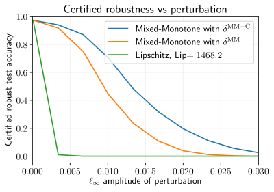
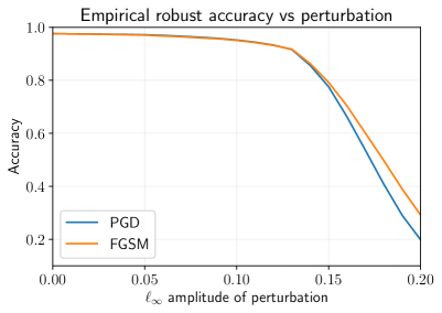
Figure 3: On the left is a plot of the certified adversarial robustness of the trained NEMON model using a Lipschitz method and two mixed monotonicity methods. For fixed $\epsilon$, the fraction of test inputs which are certified robust are plotted. On the right is a plot of the empirical robustness of the same NEMON model subject to PGD and FGSM attacks. Note the difference in scale on the horizontal axis.

5.2 MNIST experiment

In this section, we compare the certified adversarial robustness of different approaches on the MNIST handwritten digit dataset, a dataset of $70000$ $28\times 28$ pixel images, $60000$ of which are for training, and $10000$ for testing. Pixel values are normalized in $[0,1]$. We trained a fully-connected NEMON model, introduced in (Jafarpour et al., 2021), with $n=100$ neurons as in the training problem (3). For well-posedness, we imposed $\mu_{\infty,[\eta]^{-1}}(A)\leq 0$, where we directly parametrize the set of such $A$ as $A=[\eta]^{-1}T[\eta]-\operatorname{diag}(|T|\mathbbold{1}_{n})$ for unconstrained $T$ (Jafarpour et al., 2021, Lemma 9). We also use the estimate in (Jafarpour et al., 2021, Corollary 5) for the input-output Lipschitz bound of the NEMON model. Training data was broken up into batches of $100$ and the model was trained for $15$ epochs with a learning rate of $10^{-3}$. After training, the model was validated on test data using the sufficient conditions for certified adversarial robustness in the previous section. For fixed $\epsilon$ and the $10000$ test images, over $10$ trials, it took, on average, $2.250$ seconds to compute $\delta^{\textup{Lip}}(\epsilon,u)$, $218.099$ seconds to compute $\delta^{\textup{IBP}}(\epsilon,u)$, $9.087$ seconds to compute $\delta^{\textup{MM}}(\epsilon,u)$, and $11.291$ seconds to compute $\delta^{\textup{MM-C}}(\epsilon,u)$. To provide a conservative upper-bound on the certified adversarial robustness and to observe empirical robustness, the model was additionally attacked using projected gradient descent (PGD) and fast-gradient sign method (FGSM) attacks. Results from these experiments are shown in Figure 3.

Summary evaluation.

We draw several conclusions from the experiments. First, the bounds on the certified adversarial robustness provided from the interval-bound propagation are not plotted since they provided a trivial lower bound of zero adversarial robustness for every $\epsilon$ tested. Second, we see that the bounds on the certified adversarial robustness provided by the mixed monotonicity approaches are tighter than the bounds provided by the Lipschitz constant. Third, we note the additional tightness in the bounds provided by computing the relative classifier variable $\underline{z}^{u}$. Finally, we observe that although mixed monotonicity approaches provide better bounds than the better-known Lipschitz and interval-bound propagation approaches, the gap between the certified robustness and the empirical robustness remains sizable, especially for larger $\ell_{\infty}$-perturbations.

6 Conclusions

Using mixed monotone systems theory and contraction theory, we developed a framework for studying robustness of implicit neural networks. A key tool in this approach is an embedded network that provides $\ell_{\infty}$-norm box estimates for input-output behavior of the given implicit neural network. Empirical evidence shows our approach outperforms existing methods. Future work includes (i) applying the mixed monotone contractive approach to other implicit neural networks such as MON (Winston and Kolter, 2020) and LBEN (Revay et al., 2020) and (ii) designing appropriate state transformations (Abate and Coogan, 2021) to improve the input-output bounds in Theorem 4.1.

References

• Abate and Coogan (2020) M. Abate and S. Coogan. Computing robustly forward invariant sets for mixed-monotone systems. In IEEE Conf. on Decision and Control, pages 4553–4559, 2020. 10.1109/CDC42340.2020.9304461.
• Abate and Coogan (2021) M. Abate and S. Coogan. Improving the fidelity of mixed-monotone reachable set approximations via state transformations. In 2021 American Control Conference (ACC), pages 4674–4679, 2021. 10.23919/ACC50511.2021.9483264.
• Abate et al. (2021) M. Abate, M. Dutreix, and S. Coogan. Tight decomposition functions for continuous-time mixed-monotone systems with disturbances. IEEE Control Systems Letters, 5(1):139–144, 2021. 10.1109/LCSYS.2020.3001085.
• Angeli and Sontag (2003) D. Angeli and E. D. Sontag. Monotone control systems. IEEE Transactions on Automatic Control, 48(10):1684–1698, 2003. 10.1109/TAC.2003.817920.
• Angeli et al. (2014) D. Angeli, G. A. Enciso, and E. D. Sontag. A small-gain result for orthant-monotone systems under mixed feedback. Systems & Control Letters, 68:9–19, 2014. 10.1016/j.sysconle.2014.03.002.
• Anonymous (2022) Anonymous. Certified robustness for deep equilibrium models via interval bound propagation. In Submitted to The Tenth International Conference on Learning Representations, 2022. URL https://openreview.net/forum?id=y1PXylgrXZ. under review.
• Athalye et al. (2018) A. Athalye, L. Engstrom, A. Ilyas, and K. Kwok. Synthesizing robust adversarial examples, 2018. URL https://openreview.net/forum?id=BJDH5M-AW.
• Bai et al. (2019) S. Bai, J. Z. Kolter, and V. Koltun. Deep equilibrium models. In Advances in Neural Information Processing Systems, 2019. URL https://arxiv.org/abs/1909.01377.
• Blum et al. (2020) A. Blum, T. Dick, N. Manoj, and H. Zhang. Random smoothing might be unable to certify $\ell_{\infty}$ robustness for high-dimensional images. Journal of Machine Learning Research, 21(211):1–21, 2020. URL http://jmlr.org/papers/v21/20-209.html.
• Bullo et al. (2021) F. Bullo, P. Cisneros-Velarde, A. Davydov, and S. Jafarpour. From contraction theory to fixed point algorithms on Riemannian and non-Euclidean spaces. In IEEE Conf. on Decision and Control, December 2021. URL https://arxiv.org/pdf/2110.03623. To appear (Invited Tutorial Session).
• Carlini and Wagner (2017) N. Carlini and D. Wagner. Adversarial examples are not easily detected: Bypassing ten detection methods. In ACM Workshop on Artificial Intelligence and Security, pages 3–14, 2017. 10.1145/3128572.3140444.
• Chen et al. (2021) T. Chen, J. B. Lasserre, V. Magron, and E. Pauwels. Semialgebraic representation of monotone deep equilibrium models and applications to certification. In Thirty-Fifth Conference on Neural Information Processing Systems, 2021. URL https://openreview.net/forum?id=m4rb1Rlfdi.
• Cohen et al. (2019) J. Cohen, E. Rosenfeld, and J. Z. Kolter. Certified adversarial robustness via randomized smoothing. In Int. Conf. on Machine Learning, pages 1310–1320, 2019. URL https://arxiv.org/abs/1902.02918.
• Combettes and Pesquet (2020) P. L. Combettes and J-C. Pesquet. Lipschitz certificates for layered network structures driven by averaged activation operators. SIAM Journal on Mathematics of Data Science, 2(2):529–557, 2020. 10.1137/19M1272780.
• Coogan (2020) S. Coogan. Mixed monotonicity for reachability and safety in dynamical systems. In 2020 59th IEEE Conference on Decision and Control (CDC), pages 5074–5085, 2020. 10.1109/CDC42340.2020.9304391.
• Coogan and Arcak (2015) S. Coogan and M. Arcak. Efficient finite abstraction of mixed monotone systems. In Hybrid Systems: Computation and Control, pages 58–67, April 2015. 10.1145/2728606.2728607.
• Davydov et al. (2021) A. Davydov, S. Jafarpour, and F. Bullo. Non-Euclidean contraction theory for robust nonlinear stability. IEEE Transactions on Automatic Control, July 2021. URL https://arxiv.org/abs/2103.12263. Submitted.
• El Ghaoui et al. (2021) L. El Ghaoui, F. Gu, B. Travacca, A. Askari, and A. Tsai. Implicit deep learning. SIAM Journal on Mathematics of Data Science, 3(3):930–958, 2021. 10.1137/20M1358517.
• Enciso et al. (2006) G. A. Enciso, H. L. Smith, and E. D. Sontag. Nonmonotone systems decomposable into monotone systems with negative feedback. Journal of Differential Equations, 224(1):205–227, 2006. 10.1016/j.jde.2005.05.007.
• Farina and Rinaldi (2000) L. Farina and S. Rinaldi. Positive Linear Systems: Theory and Applications. John Wiley & Sons, 2000. ISBN 0471384569.
• Fazlyab et al. (2019) M. Fazlyab, A. Robey, H. Hassani, M. Morari, and G. J. Pappas. Efficient and accurate estimation of Lipschitz constants for deep neural networks. In Advances in Neural Information Processing Systems, 2019. URL https://arxiv.org/abs/1906.04893.
• Goodfellow et al. (2015) I. J. Goodfellow, J. Shlens, and C. Szegedy. Explaining and harnessing adversarial examples. In International Conference on Learning Representations (ICLR), 2015. URL https://arxiv.org/abs/1412.6572.
• Gowal et al. (2018) S. Gowal, K. Dvijotham, R. Stanforth, R. Bunel, C. Qin, J. Uesato, R. Arandjelovic, T. Mann, and P. Kohli. On the effectiveness of interval bound propagation for training verifiably robust models. arXiv preprint arXiv:1810.12715, 2018.
• Jafarpour et al. (2021) S. Jafarpour, A. Davydov, A. V. Proskurnikov, and F. Bullo. Robust implicit networks via non-Euclidean contractions. In Advances in Neural Information Processing Systems, December 2021. URL http://arxiv.org/abs/2106.03194.
• Kag et al. (2020) A. Kag, Z. Zhang, and V. Saligrama. RNNs incrementally evolving on an equilibrium manifold: A panacea for vanishing and exploding gradients? In International Conference on Learning Representations, 2020. URL https://openreview.net/forum?id=HylpqA4FwS.
• Li et al. (2019) B. Li, C. Chen, W. Wang, and L. Carin. Certified adversarial robustness with additive noise. In Advances in Neural Information Processing Systems, 2019. URL https://arxiv.org/abs/1809.03113.
• Madry et al. (2018) A. Madry, A. Makelov, L. Schmidt, D. Tsipras, and A. Vladu. Towards deep learning models resistant to adversarial attacks. In International Conference on Machine Learning, 2018. URL https://arxiv.org/abs/1706.06083.
• Mirman et al. (2018) M. Mirman, T. Gehr, and M. Vechev. Differentiable abstract interpretation for provably robust neural networks. In J. Dy and A. Krause, editors, Proceedings of the 35th International Conference on Machine Learning, volume 80 of Proceedings of Machine Learning Research, pages 3578–3586. PMLR, 10-15 Jul 2018. URL https://proceedings.mlr.press/v80/mirman18b.html.
• Pabbaraju et al. (2021) C. Pabbaraju, E. Winston, and J. Z. Kolter. Estimating Lipschitz constants of monotone deep equilibrium models. In International Conference on Learning Representations, 2021. URL https://openreview.net/forum?id=VcB4QkSfyO.
• Papernot et al. (2016) N. Papernot, P. McDaniel, X. Wu, S. Jha, and A. Swami. Distillation as a defense to adversarial perturbations against deep neural networks. In IEEE Symposium on Security and Privacy (SP), pages 582–597, 2016. 10.1109/SP.2016.41.
• Revay et al. (2020) M. Revay, R. Wang, and I. R. Manchester. Lipschitz bounded equilibrium networks. 2020. URL https://arxiv.org/abs/2010.01732.
• Smith (1995) H. L. Smith. Monotone Dynamical Systems: An Introduction to the Theory of Competitive and Cooperative Systems. American Mathematical Society, 1995. ISBN 082180393X.
• Szegedy et al. (2014) C. Szegedy, W. Zaremba, I. Sutskever, J. Bruna, D. Erhan, I. Goodfellow, and R. Fergus. Intriguing properties of neural networks. In International Conference on Learning Representations, 2014. URL https://arxiv.org/abs/1312.6199.
• Virmaux and Scaman (2018) A. Virmaux and K. Scaman. Lipschitz regularity of deep neural networks: analysis and efficient estimation. In Advances in Neural Information Processing Systems, volume 31, page 3839–3848, 2018. URL https://proceedings.neurips.cc/paper/2018/file/d54e99a6c03704e95e6965532dec148b-Paper.pdf.
• Winston and Kolter (2020) E. Winston and J. Z. Kolter. Monotone operator equilibrium networks. In Advances in Neural Information Processing Systems, 2020. URL https://arxiv.org/abs/2006.08591.
• Wong and Kolter (2018) E. Wong and J. Z. Kolter. Provable defenses against adversarial examples via the convex outer adversarial polytope. In International Conference on Machine Learning, pages 5286–5295, 2018. URL http://proceedings.mlr.press/v80/wong18a.html.
• Yang and Ozay (2019) L. Yang and N. Ozay. Tight decomposition functions for mixed monotonicity. In 2019 IEEE 58th Conference on Decision and Control (CDC), pages 5318–5322, 2019. 10.1109/CDC40024.2019.9030065.
• Zhang et al. (2018) H. Zhang, T-W. Weng, P-Y. Chen, C-J. Hsieh, and L. Daniel. Efficient neural network robustness certification with general activation functions. In Advances in Neural Information Processing Systems, page 4944–4953, 2018. URL https://arxiv.org/abs/1811.00866.
• Zhang et al. (2020) H. Zhang, H. Chen, C. Xiao, S. Gowal, R. Stanforth, Bo Li, D. Boning, and C-J. Hsieh. Towards stable and efficient training of verifiably robust neural networks. In International Conference on Learning Representations, 2020. URL https://openreview.net/forum?id=Skxuk1rFwB.