Eigenfunction and eigenmode-spacing statistics in chaotic photonic crystal graphs

Abstract

The statistical properties of wave chaotic systems of varying dimensionalities and realizations have been studied extensively. These systems are commonly characterized by the statistics of the eigenmode-spacings and the statistics of the eigenfunctions. Here, we propose photonic crystal (PC) defect waveguide graphs as a new physical setting for chaotic graph studies. Photonic crystal waveguides possess a dispersion relation for the propagating modes which is engineerable. Graphs constructed by joining these waveguides possess junctions and bends with distinct scattering properties. We present numerically determined statistical properties of an ensemble of such PC-graphs including both eigenfunction amplitude and eigenmode-spacing studies. Our proposed system is compatible with silicon nanophotonic technology and opens chaotic graph studies to a new community of researchers.

I I. Introduction

Wave-chaotic phenomena have been studied in various complex scattering systems, ranging from 1D graphs Hul et al. (2004); Martínez-Argüello et al. (2018); Rehemanjiang et al. (2020); Lu et al. (2020); Chen et al. (2020), 2D billiards Wu et al. (1998); Dembowski et al. (2003, 2005); Hemmady et al. (2005); Kuhl et al. (2008); Shinohara et al. (2010); Dietz and Richter (2019) to 3D enclosures Hemmady et al. (2012); Xiao et al. (2018); Ma et al. (2019a, 2020a, 2020b); Frazier et al. (2020). The statistical properties of many system quantities, such as the closed system eigenvalues and the open system scattering/impedance matrices, exhibit universal characteristics, which only depend on general symmetries (e.g., time-reversal, symplectic) and the degree of system loss. Random Matrix Theory (RMT) has enjoyed great success in describing the energy level spacing statistics of large nuclei Mehta (2004); Dietz et al. (2017a). The statistics of complex systems that show time-reversal invariance (TRI) are described by the Gaussian orthogonal ensemble (GOE) of random matrices, and the statistics of systems showing broken time-reversal invariance are described by the Gaussian unitary ensemble (GUE), and the statistics of systems with TRI and antiunitary symmetry show Gaussian symplectic ensemble (GSE) statistics So et al. (1995); Hemmady et al. (2005); Ma et al. (2020a). It was later conjectured by Bohigas, Giannoni, and Schmit that any system with chaotic dynamics in the classical limit would also have semi-classical wave properties whose statistics are governed by RMT associated with one of these three ensembles Bohigas et al. (1984). In practice, identifying RMT statistical properties in experimental data is difficult due to the presence of non-universal features that obscure the universal fluctuations. The Random Coupling Model (RCM) has found great success in characterizing the statistical properties of a variety of experimental systems by removing the non-universal effects induced by port coupling and short-orbit effects Hemmady et al. (2005); Zheng et al. (2006); Hart et al. (2009); Yeh et al. (2010); Hemmady et al. (2012); Li et al. (2015); Aurégan and Pagneux (2016); Xiao et al. (2018); Zhou et al. (2019); Ma et al. (2020a, b).

Chaotic microwave graphs support complex scattering phenomena despite their relatively simple structure Hul et al. (2004); Martínez-Argüello et al. (2018); Rehemanjiang et al. (2020); Lu et al. (2020); Chen et al. (2020); Zhang et al. (2022). We refer loosely to a chaotic graph as one in which there are multiple paths of differing lengths from one node to another, such that waves traveling along these paths interfere when arriving at nodes. A microwave graph structure can be realized with coaxial cables as graph bonds connected at T-junctions. The graph architecture allows for various useful circuit components (such as variable phase shifters and attenuators, as well as microwave circulators) to be incorporated into the structure Rehemanjiang et al. (2020); Lu et al. (2020); Chen et al. (2020). Recent studies show that non-universal statistical features exist in chaotic graph systems, and these are hypothesized to be caused by the non-zero reflection at the graph vertices. These reflections create trapped modes that impact the spectral statistics of the graph Białous et al. (2016); Dietz et al. (2017b); Lu et al. (2020); Che et al. (2021).

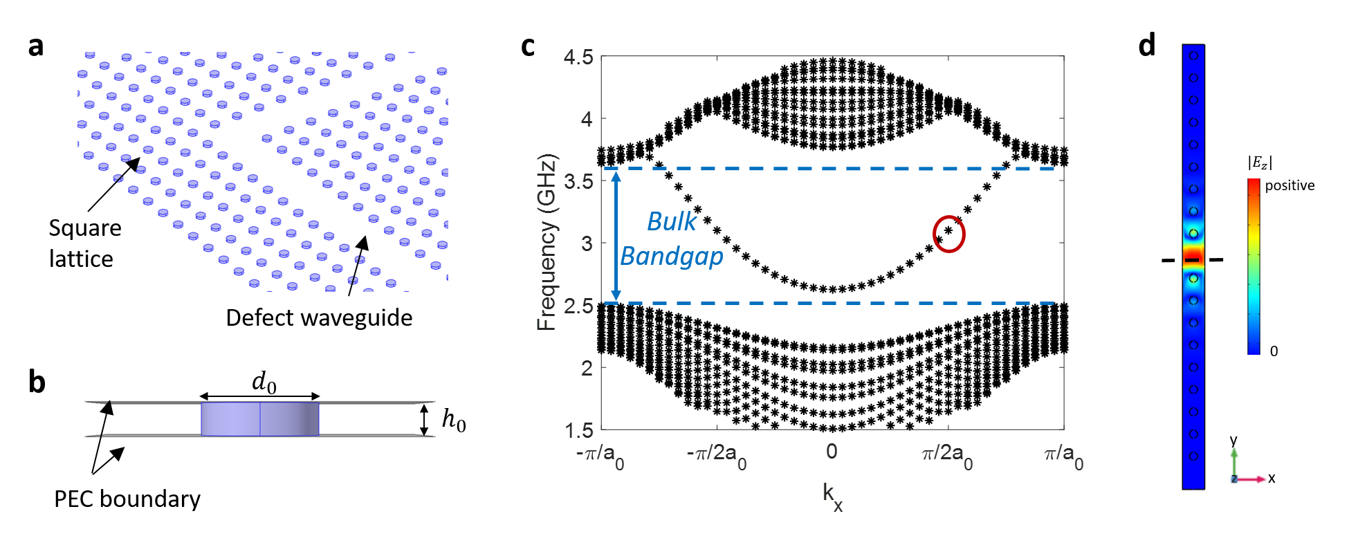
Figure 1: a. The open-plate view of the photonic crystal lattice with an L-shaped defect waveguide region. b. The side view of the PC unit cell. A dielectric rod is sandwiched between two PEC (perfect electric conductor) surfaces. The quantities $h_{0}$ and $d_{0}$ are the height and diameter of the rod. c. The photonic band structure from a supercell defect waveguide simulation. The waveguide modes appear in the bulk bandgap region (delineated by the blue dashed lines). d. The E-field profile of one of the waveguide mode solutions (the red circle in c). The black dashed line marks the center of the waveguide.

Here, we introduce an alternative type of chaotic graph built with photonic crystal (PC) waveguides. Photonic crystals find extensive use in semiconductor-based nanophotonic technology, where they act as low-loss waveguides for visible and infrared light Johnson et al. (2001). The PC graph bonds are realized with defect waveguides, and the nodes are formed by the waveguide junctions. As TRI is preserved and spin-1/2 behavior is absent, chaotic PC-graph systems are expected to fall into the GOE universality class of RMT. With numerical simulation tools, we conduct a series of statistical tests of chaotic photonic crystal graph systems including both eigenvalue and eigenfunction studies of closed graphs.

The unique properties of PC structures for quantum chaos studies are as follows. First, the bond lengths of PC-graphs can be altered by means of lithographic fabrication Johnson et al. (2001). Second, the scattering properties of PC-graph nodes can be engineered by changing the rod properties and geometry. Moreover, PC defect waveguides and cavities are technologies that are widely used in the field of integrated nanophotonics. To our knowledge, PC waveguide graphs have not been previously utilized for quantum graph studies.

The paper is organized as follows. In Section II, we introduce the design details of the proposed PC graph structure as well as its numerical implementation methods. We present the chaotic closed-graph mode-spacing study in section III, and focus on the discussion of closed-graph eigenfunction studies in section IV. Different methods of conducting eigenfunction statistical studies are also discussed. We summarize the paper and discuss the future applications of the proposed PC graphs in section V.

II II. Photonic crystal graph

A photonic crystal system consists of a regular lattice of artificial atoms (or scatterers) whose spacing is comparable to the operating wavelength Joannopoulos et al. (1997, 2008). The material properties and the geometrical details of the atoms are carefully designed in order to achieve a specific functionality. A PC system is usually constructed as a 2D planar structure, which makes it especially good for lithographic fabrication and photonics applications. Importantly, a 2D PC can show a complete bulk bandgap in its electromagnetic excitation spectrum Joannopoulos et al. (1997, 2008). In PC-based devices, waveguides and cavities can be constructed for example by making air defects (removing a certain number of the atoms) in the original lattice. This creates guided propagating modes in the bulk bandgap, which ensures that the modes are confined to the defect region. A variety of defect waveguides can be realized by changing the atom properties Joannopoulos et al. (1997). Recent photonic topological insulator (PTI) studies present an alternative form of PC waveguide using the interface between two different topological domains Xiao et al. (2016); Lai et al. (2016); Ma et al. (2019b); Ma and Anlage (2020); Liu et al. (2021). Such PTI-based waveguides can also be utilized as the bonds for realizing graphs. The interesting properties of the topologically protected modes may further enhance the quantum graph studies. Here, we will utilize the defect waveguide modes to build chaotic graph structures. Note that these PC defect waveguide graphs are distinctly different from photonic crystal slabs and billiards Dietz and Richter (2019); Maimaiti et al. (2020); Zhang and Dietz (2021), and from coupled resonant dielectric cylinders Rehemanjiang et al. (2020); Reisner et al. (2021) studied previously.

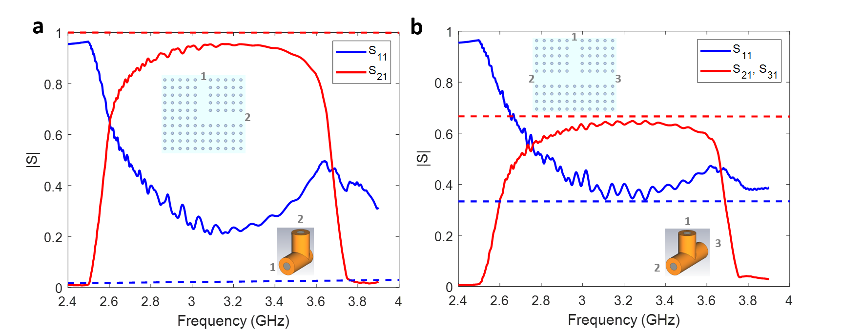
Figure 2: a. The simulated S-parameters of the PC-graph right-angle junction (solid), as well as the S-parameter from a $3.5mm$ uniform coaxial cable 2-port right-angle connector (dashed), which serves as a reference. Inset: the schematics of the PC right-angle junction and the 2-port coaxial cable junction. b. The simulated S-parameters of the PC-graph T-junction (solid) and the S-parameters from a coaxial cable 3-port ‘T’ connector (dashed). Inset: schematics of the PC T-junction and the 3-port coaxial cable junction. All PC-junction S-parameters are frequency averaged with a 500MHz window to remove the effect of spurious reflections.

The construction of the chaotic PC graph starts by building a square lattice with identical dielectric rods (the blue lattice in Fig. 1(a)). The lattice constant is $a_{0}=36.8mm$. The dielectric rod lattice is located between two metallic surfaces and installed in a vacuum background. The defect waveguide is created by simply removing one row or column of the dielectric rods. The detailed shape of the dielectric rod is shown in Fig. 1(b). The diameter of the dielectric rod is $d_{0}=0.36a_{0}=13.2mm$ and the height is $h_{0}=0.1a_{0}=3.68mm$. Because the PC lattice is thin in the vertical direction ($z$-direction), the waveguide modes considered here are polarized such that $E_{z}\neq 0$, $E_{x,y}=0$, $H_{z}=0$ and $H_{x,y}\neq 0$ (TM with respect to $z$), and these are the only modes that propagate for frequencies $f<12$ GHz, well above the band gap of interest here. The relative permitivity and permeability of the dielectric rods are $\epsilon_{r}=11.56$ and $\mu_{r}=1$. We realize the proposed PC structure numerically with COMSOL Multiphysics Software. The presence of the waveguide mode is clearly demonstrated by the supercell photonic band structure (PBS) simulation (Fig. 1(c)). The supercell simulation model consists of a single column of PC lattice with Floquet periodic boundaries on the two long sides. That is, fields on opposite long sides differ by a phase factor $\theta=k_{x}a_{0}$. Fields on the opposite short sides are assigned totally absorbing boundary conditions. We remove the center rod to create the defect waveguide region. The PBS simulation is conducted by computing the system eigenmodes while varying the wavenumber $k_{x}$ in the range $[-\pi/a_{0},\pi/a_{0}]$. As shown in Fig. 1(c), the defect waveguide modes have emerged inside of the bulk bandgap region from $2.5\sim 3.6$GHz. The eigenfrequencies in the band-gap region are essentially real, as the absorbing boundaries are well separated from the defect creating the waveguide.

We see from Fig. 1(c) that the waveguide modes in the PC have a distinct dispersion relation (frequency versus $k_{x}$) that differs from that of a transmission line, $\omega=k_{x}c$. The dispersion relation is parabolic at the lower band-edge, as in a metallic waveguide. However, the group velocity vanishes at the upper band-edge, in contrast with that of a metallic waveguide for which there is no upper band-edge, rather just a boundary where new propagating modes are possible Zhang et al. (2022). In Fig. 1(d), the $|E_{z}|$ profile of the entire simulation domain shows clearly that the mode solution is indeed a guided wave because its amplitude is highly localized in the defect region.

In addition to the propagation on the graph bonds, it is also important to characterize the scattering properties of graph nodes Bittner et al. (2013). The PC graph structure is realized by connecting multiple straight defect waveguides with both right-angle and T-shaped junctions. We have characterized the scattering matrix of both types of junctions with COMSOL and CST Microwave STUDIO. For the right-angle junctions, non-zero transmission is found only in the bulk bandgap region. As shown in Fig. 2(a), the transmission $|S_{21}|$ and the reflection $|S_{11}|$ for right angle bends vary systematically as functions of frequency. Thus, right-angle bends are vertices with a non-trivial scattering matrix in a graph. The PC-graph T-junction also presents a complex scattering profile over the entire bandgap region. As shown in Fig. 2(b), the magnitude of the reflection (transmission) coefficient deviates systematically from 1/3 (2/3) as a function of frequency.

It should be noted that for the PC graph junctions the sum of the squares of the displayed scattering coefficients is close to unity. This implies that at the frequencies of interest the photonic waveguides are operating in a single transverse mode. For an ideal transmission line there is no reflection at a bend. Also, at an ideal T-junction the reflection coefficient $|S_{11}|=|-1/3|$, and the transmission coefficient is $|S_{12}|=|2/3|$. The ideal scattering parameters apply to transmission lines whose transverse dimensions are much smaller than an axial wavelength (equivalently the frequency is well below the first cut-off frequency of non-TEM modes.). The calculated scattering properties of an air-filled coaxial ($r_{o}=2$ mm, $r_{i}=0.86$ mm) cable bend and T-junction are shown as well in Fig. 2, and, by contrast, they show minimal variation in the frequency range of interest. The cut-off frequency of the $TE_{11}$ mode in this cable is 33.34 GHz, well above the operating frequency. Consequently, the scattering parameters are close to the ideal values. Graphs constructed of metallic waveguides, as opposed to transmission lines, can be expected to have scattering parameters with characteristics similar to PC graphs for frequencies between the first and second lowest cut-off frequencies where single mode operation is possible Zhang et al. (2022). These nontrivial junction scattering parameters are a second unique feature of PC graphs, and can be expected to influence the properties of the graph eigenmodes. We note that alternative methods of making waveguide bends, or connecting waveguides, can be applied, for example by removing or adding dielectric rods at the right-angle turn, in order to tune the transmission property of the waveguide joints Mekis et al. (1996). One may adjust the degree of wave localization of graph nodes by engineering the scattering properties of the PC waveguide junctions. The engineering of the node reflection and transmission properties is beyond the scope of this paper.

We simulate the closed PC graphs with the COMSOL eigenvalue solver. The graph topology is that of a flattened tetrahedral graph having $14$ straight segments and $13$ junctions (including both 3-way junctions and right-angle junctions). The four exterior faces of the parallel-plate PC structure (see Fig. 3(a)) are assigned totally absorbing boundary conditions. The total length of the simulated graph is on the scale of $\sim 9$ m, which hosts about 80 eigenmodes (within the bulk PC bandgap) in a typical realization. We note that one is able to decrease the mode-spacing by enlarging the size of the PC graph, and we choose the current system scale due to limited computational power. We have created a statistical ensemble of chaotic PC graphs by changing the length of the bonds for a given graph topology.

A particular eigenmode solution of a graph (shown in Fig. 3(a)) is shown in Fig. 3(b). It is clear that the graph mode is localized to the defect waveguide region and displays a longitudinal sinusoidal standing wave pattern. The mode amplitude on a single bond is uniform but varies between different bonds (shown by the color differences), where bonds are defined as straight waveguide regions between 3-way junctions and right-angle bends.

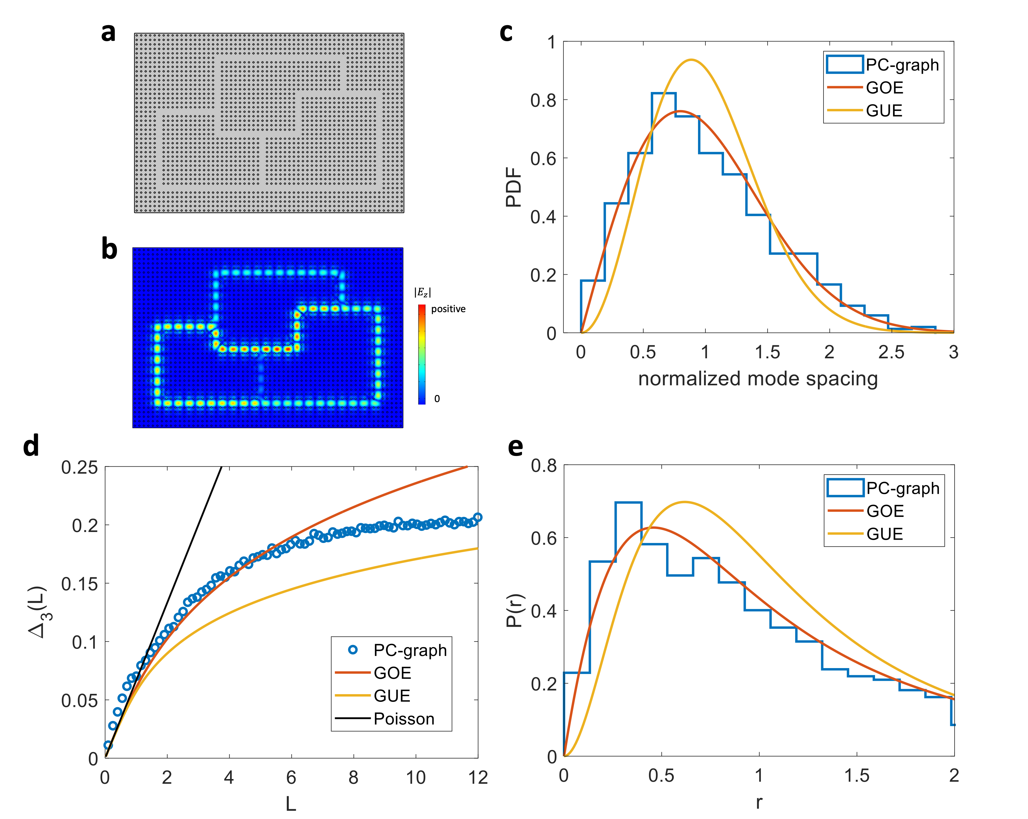
Figure 3: a. Schematic diagram of the PC waveguide graph system. The graph bonds are shown as clear gray channels, and the rectangular lattice is shown as a lattice of dielectric rods (black circles). b. The simulated $|E_{z}|$ profile of the graph system eigenmode at 2.8GHz. c shows the statistics of the normalized mode spacing from graph simulation (histogram). The theoretical predictions for the GOE and GUE systems are shown in red and yellow curves. d shows the spectral rigidity $\Delta_{3}(L)$ of the normalized spectrum from graph simulation (blue circles). The theoretical predictions for the GOE, GUE, and the Poisson systems are shown in red, yellow, and black curves. e shows the statistics of the consecutive mode spacing ratio $r$ (histogram) and the theoretical predictions for the GOE and GUE systems.

III III. Eigenmode Spacing Statistical Analysis

In order to characterize the statistical properties of PC defect waveguide graphs, we start by conducting the nearest neighbor mode spacing analysis of the proposed PC graphs. An ensemble of 10 different graph realizations is studied numerically, and we obtained $\sim 800$ eigenfrequency values from the ensemble. The graph topology ranges from $13\sim 16$ straight segments and $11\sim 14$ junctions. We note that this ensemble of graphs is conducted with the eigenvalue simulation in COMSOL. The simulation results are used for mode-spacing studies here, as well as the eigenfunction statistics in Sec. IV. The model is composed of lossless dielectric structures. However, the presence of radiating boundary conditions on the perimeter of the finite-size structure shown in Fig. 3(a) will give rise to a finite loss. The quality factors of the simulated graph modes are on the order of $10^{5}$ to $10^{7}$, allowing for clear identification of all eigenfrequencies. The graph topology is kept fixed in the eigenfunction studies discussed below. Because the topology and the total length $L_{tot}$ of each graph realization are different, we normalized the system eigenmode solutions using the following method. We considered 10 different graphs. For each graph, we calculated eigenfrequencies in the range 2.8 GHz to 3.6 GHz and placed the eigenfrequencies in ascending order. The eigenfrequencies were then converted to eigen-wavenumbers ($k_{i}$, $i$ is the mode index) using the dispersion relation for the PC-waveguide PBS shown in Fig. 1(c). This results in a tabulation of consecutive wave-numbers. We then fit the mode-number index to the wave-number using a quadratic fitting function $n(k)=c_{2}k^{2}+c_{1}k+c_{0}$, where $c_{0,1,2}$ are fitting parameters and $n(k)$ is the total number of modes below $k$ Rehemanjiang et al. (2016). For a typical graph we found $c_{2}=0.0054m^{2},c_{1}=2.21m$ and $c_{0}=-55.28$. The small value of $c_{2}$ indicates the $n(k)$ is nearly linear in $k$ as expected for quasi-one-dimensional structures. We then evaluate the fitting functions at the calculated $k$-values for each graph, creating a list of normalized eigenvalues $e_{i}=n_{fit}(k_{i})$. The nearest neighbor spacings are finally computed as $s_{i}=e_{i+1}-e_{i}$.

The distribution of the normalized nearest-neighbor mode spacing values of the entire ensemble is shown as the histogram in Fig. 3(c). We have included the approximate theoretical predictions of the mode-spacing statistics for the GOE and GUE systems in the figure. These theoretical predictions are based on RMT Berry (1981); Kottos and Smilansky (1997, 1999), which are methods of understanding the universal statistical properties of wave-chaotic systems Casati et al. (1980); Bohigas et al. (1984). As shown in Fig. 3(c), the distribution of the normalized mode-spacing matches reasonably well with the theoretical prediction for the GOE universality class. Good agreement between the graph nearest neighbor mode-spacing statistics and the RMT theoretical prediction is also reported in various works on graphs, although long-range statistical quantities tend to show non-universal behavior due to the trapped-mode issue mentioned above Białous et al. (2016); Dietz et al. (2017b); Lu et al. (2020); Che et al. (2021).

To test the long-range statistical properties of the eigenmodes, we compute the spectral rigidity of the graph spectrum $\Delta_{3}(L)$, where $L$ measures the length of a segment in the normalized spectrum. Our procedure is as follows. The quantity $\Delta_{3}(e,L)$ representing the deviation of the spectral staircase from a straight line, is evaluated for each value of $L$ by

$$\Delta_{3}(e,L)=\frac{1}{L}min_{a,b}\int_{e}^{e+L}[N(x)-ax-b]^{2}dx,$$ (1)

where $N(e)=n(k)$ and $e$ is chosen at random. We use 100 values of e for each graph. Then we average the values of e over 10 graph realizations Haq et al. (1982). The resulting values of $\Delta_{3}(e,L)$ are then plotted in Fig. 3(d) along with theoretical predictions based on GOE, and GUE random matrices Che et al. (2021), and the predictions of Poisson statistics Berry (1985) (appropriate for classically integrable systems).

The $\Delta_{3}(L)$ curve in Fig. 3(d) is linear in $L$ for small values of $L$. As shown, systems of all symmetries (Poisson, GOE, GUE) show a linear-in-$L$ dependence for $L<1$ Berry (1985), and the data is consistent with this trend. Chaotic systems are then expected to show a logarithmic increase in $\Delta_{3}(L)$ Berry (1985), and this is evident in the data up to approximately $L=5$. It is also predicted that $\Delta_{3}(L)$ will saturate due to the presence of short orbits in any experimental realization of a wave chaotic system Berry (1985), and this is also seen in the data. Previous studies find that the long-range statistics of quantum graphs usually show some degree of agreement with the GOE prediction in the range of roughly $L\in[2,5]$, along with deviations beyond this range Hul et al. (2004); Białous et al. (2016); Dietz et al. (2017b). We observe in Fig. 3(d) a deviation from the GOE RMT predictions, especially for larger $L$, similar to cable graph studies in Ref. Hul et al. (2004). Because the operating bandwidth of the proposed PC-graph system is relatively narrow (Fig. 1 (c)), we believe the long-range statistics may also be affected by finite-size effects because the number of available eigenmodes is bounded above and below by the edge of the PC bandgap. The solution is to increase the graph size substantially, but this is beyond our computational resources. In summary, the $\Delta_{3}(L)$ behavior is very similar to that observed in wave chaotic systems of higher dimensionality.

	PC-Graph	GOE	GUE	GSE
$\left<r\right>$	1.89	1.75	1.37	1.18
$\left<\tilde{r}\right>$	0.51	0.54	0.60	0.68

Table 1: The summarized consecutive mode spacing ratios of the photonic crystal graph (PC-Graph) system, and the theoretical predictions for the GOE, GUE, and GSE systems Atas et al. (2013).

In addition to the mode-spacing distribution test, we note that the method of consecutive mode spacing ratios $r_{i}=\frac{s_{i}}{s_{i-1}}$ and $\tilde{r}_{i}=min\left(r_{i},\frac{1}{r_{i}}\right)$ can also be adopted Atas et al. (2013). Here the ratio statistic has the feature that it is a measure of the correlation between adjacent spacings. One advantage of this type of statistical study is that it does not require unfolding the spectrum Atas et al. (2013). However, here we use the unfolded spectrum $s_{i}$ to compute the spacing ratios. For the PC graphs, the averaged values of $\left<r\right>=1.89$ and $\left<\tilde{r}\right>=0.51$, are closer to the GOE theoretical predictions than the GUE prediction (Table. 1). We note that the high value of $\left<r\right>$ in the PC-graph is related to the correlation between consecutive level-spacings. We further present the distribution of mode-spacing ratios $r$ of the PC graphs and corresponding theoretical predictions of the GOE and GUE systems in Fig. 3(e). The statistics of $r$ match reasonably well with the GOE prediction.

IV IV. Eigenfunction Analysis

We next study the statistics of the closed PC graph eigenfunctions. The eigenfunction statistics have been studied experimentally in 2D chaotic systems by probing the electromagnetic (EM) standing wave field inside a microwave cavity Kudrolli et al. (1995); Wu et al. (1998); Gokirmak et al. (1998); Chung et al. (2000); Kuhl et al. (2000); Hlushchuk et al. (2001). In those studies, the experimental probability amplitude distribution and two-point correlation function agree well with the random plane wave conjecture. Here, the wave properties of the entire closed PC graph (nodes and bonds) can be faithfully simulated. We employ the same eigenvalue simulation model used in the mode-spacing studies above. For a graph system, the telegrapher’s equation is formally equivalent to the 1D Schrödinger equation, where the wavefunction $\psi$ is represented by the wave voltage. For thin parallel plate waveguides, the wave voltage difference between the top and bottom metallic plates is represented by the $E_{z}$ value at the middle cutting plane (at the height of $z=h_{0}/2$). Because the PC graph bonds have a finite width, the bond eigenfunction will be evaluated along a 1D line at the center of the waveguide (shown as the black dashed line in Fig. 1(d)). We next examine two PC graph eigenfunction characterization methods.

Method I: grid-wise representation. For each eigenmode of each graph realization, we will use the entire set of the graph bond $|E_{z}|^{2}$ vs. longitudinal position along the center-line of the waveguide data points to represent the eigenfunction. The name ‘grid-wise’ comes from the granular nature of this method, where the total number of eigenfunction data points is inversely proportional to the computational grid size. We study the wavefunction statistics of the PC graph by computing the distribution of the normalized probability density $v$, which is defined as the square of the eigenfunction values

$$v_{j}=|\psi(r_{j})|^{2}=\frac{|E_{z}(r_{j})|^{2}\cdot L_{tot}}{\sum_{j}|E_{z}(r_{j})|^{2}\cdot\Delta L_{j}},$$ (2)

where $L_{tot}$ is the total length of the graph, $r_{j}$ and $\Delta L_{j}$ are the location and the grid size of the $j^{\prime}th$ grid point, $|E_{z}(r_{j})|$ is the z-directed electric field magnitude at the $j^{\prime}th$ grid point, and the summation in the denominator runs over every graph grid point. In our simulation, the grid size $\Delta L_{j}\sim 0.05\lambda_{op}$ where $\lambda_{op}=10cm$ is the operating wavelength at $3GHz$. The distribution of the probability density values is computed using the data from all simulated eigenmode solutions (48 to be specific) from a single realization, and the results are shown in Fig. 4(a), and discussed below.

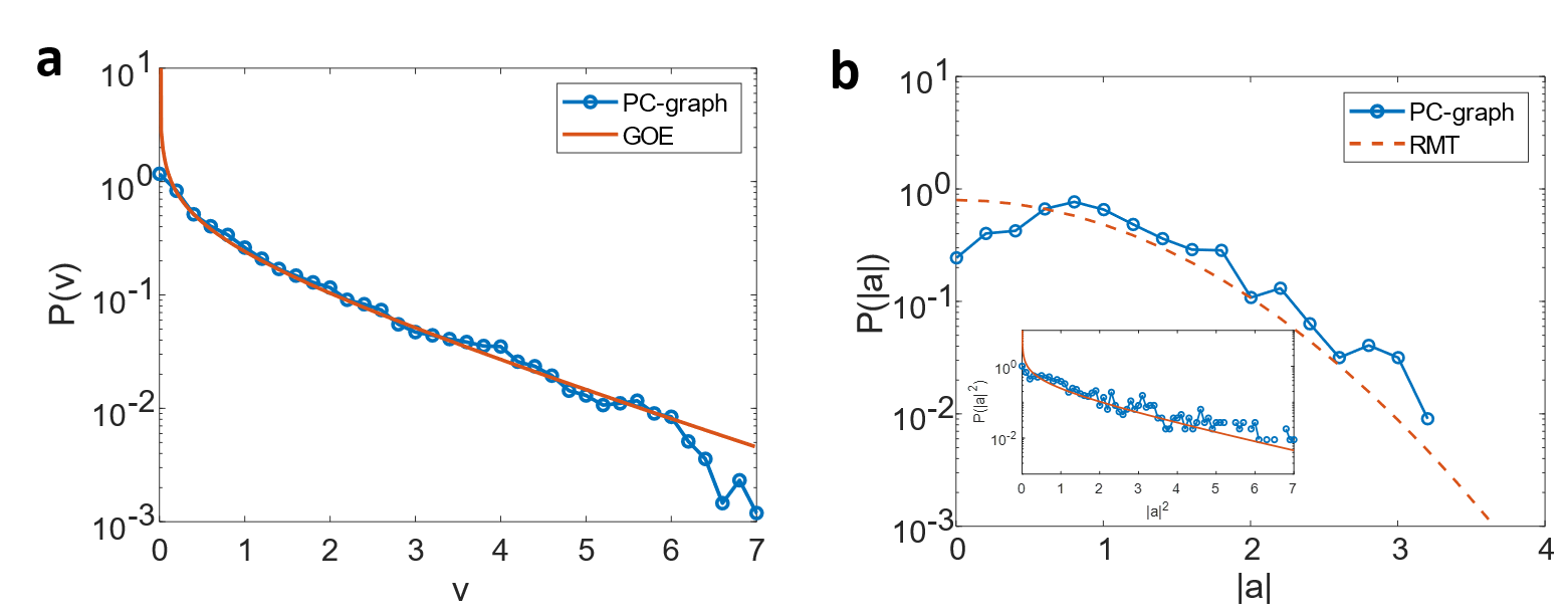
Figure 4: a. Probability amplitude distribution of photonic crystal defect waveguide graph eigenmodes values ($v$) obtained from the grid-wise method (symbols connected by blue line). The theoretical prediction for systems with GOE statistics is in red. b. shows the statistics of the normalized bond amplitude value $|a|$ (symbols connected by blue line) and the Gaussian distribution (red dashed). The inset shows the distribution of the quantity $|a|^{2}$ and the Porter-Thomas theoretical prediction for the GOE system.

Method II: bond-value representation. For each graph realization, the eigenfunction of a mode is represented by a set of ‘bond-values’ $E_{z}(b_{m})$ which is defined as the amplitude of the standing-wave wavefunction on the graph bond $b_{m}$. The quantity $m$ is the index of the bond and runs from 1 to 14. The standing wave on the bond is made up of two counter propagation waves $\psi(x)=a_{m}\,e^{ikx}+a_{m}^{*}\,e^{-ikx}$, where $a_{m}$ is the wavefunction amplitude at bond $b_{m}$ and $x$ is the distance from a vertex along the bond. We first conduct a sine-fit of the raw $E_{z}(x)$ values on each bond, which yields the amplitude, and the value of $|a_{m}|$ is obtained as 1/2 of the amplitude value. The normalization process follows the same method as in Ref. Kaplan (2001) which ensures that $\sum_{m}L(b_{m})|a_{m}|^{2}=L_{tot}$ where $L(b_{m})$ is the length of bond $b_{m}$. Here the distribution of the probability density values is computed over $14\times 78$ data points, where 14 is the number of the bonds and 78 is the number of eigenmode solutions from one graph configuration, and the results for $P(|a|)$ are shown in Fig. 4(b).

The random plane wave hypothesis underlying chaotic eigenfunction treatments asserts that the eigenfunctions in a 2D or 3D cavity can be thought of as superpositions of plane waves with random directions and random phases. Consequently, the value of an eigenfunction at any point is a sum of many random waves and is thus a zero mean Gaussian random variable Berry (1981). For systems with TRS the plane waves come in counter-propagating pairs, and the wave function is real. For systems with TRS broken, wave directions are completely random, and the wave function is complex with independent real and imaginary parts. For the PC graph the situation is changed in that at any point in the graph there are only two counter-propagating waves of equal amplitude. The amplitudes of these waves, $|a_{m}|$ will be different on the different bonds leading to statistical variations.

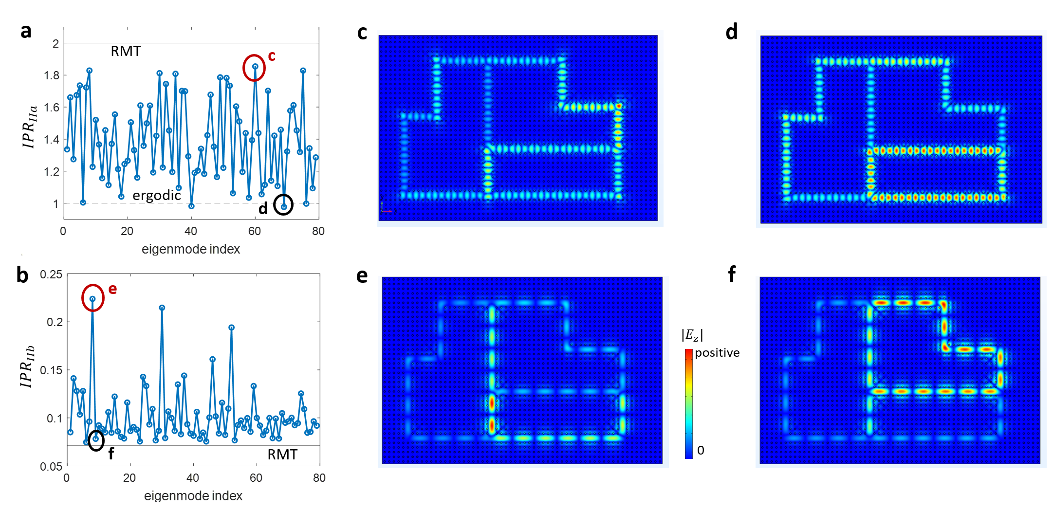
Figure 5: a. The inverse participation ratio (IPR) of graph eigenmodes obtained from the bond-value method, computed based on method IIa. The simulated $|E_{z}|$ profile of the red (black) circled mode in a is shown in c (d). b. The inverse participation ratio (IPR) of graph eigenmodes is computed based on method IIb. The simulated $|E_{z}|$ profile of the red (black) circled mode in b is shown in e (f).

We first discuss the eigenfunction statistics obtained using the grid-wise method in Fig. 4(a). For waves in a 2D or 3D cavity the distribution of values of $v$ based on the random plane wave hypothesis is $P(v)=(2\pi v)^{-1/2}e^{-v/2}$. This is shown as a solid red line in Fig. 4(a). We find that the simulated PC graph result matches to some degree the GOE prediction in that for $v>1$ the curve approaches a straight line on a log-linear plot, and for $v$ small there is an indication of square root singularity. We notice that the mismatch between the graph data and the GOE prediction exists at the small and large probability density values, indicating an absence of both very small and very large $v$ values. One possibility is that this method tends to over-count the appearance of medium-sized eigenfunction values (similar to the systematic errors experienced in Ref. Wu et al. (1998)). It may also indicate that the data simply does not match the GOE prediction. In addition to the discrete eigenfunction imaging method, we note that the eigenfunction statistics may also be tested through resonance width distributions in transmission measurements (Porter-Thomas statistics) Alt et al. (1995); Dembowski et al. (2005).

Here we now use Method II to study the distribution of normalized bond values, $|a|$ that are displayed in Fig. 4(b). Also plotted in Fig. 4(b) is a Gaussian distribution, which would be characteristic of an eigenfunction of a GOE random matrix. However, a clear deviation from Gaussian statistics is seen for low amplitudes, similar to the deviation observed with Method I. The inset to Fig. 4(b) shows a plot of $P(|a|^{2})$ compared to the Porter-Thomas distribution expected for GOE systems. There is an agreement between the two except for deviations between data and the model distribution at small values of $|a|^{2}$, similar to that seen in Fig. 4(a). Together, these results suggest that the wavefunction statistics of this simple graph are not fully consistent with the random plane wave hypothesis.

We next present the inverse participation ratio (IPR) computation based on the bond-value method (Method II) in Fig. 5. IPR is a measure of the degree of localization for a wave function Kaplan (2001); Hul et al. (2009), and can be used to quantify the degree of deviation of wavefunction statistics from the random plane wave hypothesis. Based on its IPR value, the eigenfunction behavior varies between two limits, namely the maximum ergodic limit where the wave function occupies each graph bond with equal chance, and the maximum localization limit where the eigenmode is confined to only one bond. RMT predicts an IPR value by assuming Gaussian random fluctuation of the eigenfunctions. Two different IPR definitions are tested here. Method IIa follows the definition in Ref. Kaplan (2001), where the IPR value for each graph mode is evaluated using the formula $IPR_{IIa}=\langle\left|a_{m}\right|^{4}\rangle$. As shown in Fig. 5(a), the IPR values of the photonic crystal graph modes vary erratically but lie between the maximum ergodic limit ($IPR_{IIa}$ = 1) and the RMT prediction limit ($IPR_{IIa}$ = 2) Kaplan (2001). In the maximum localization limit the $IPR_{IIa}=B$, where $B=14$ is the number of graph bonds, and the results are far from this limit. Method IIb follows the definition in Ref. Hul et al. (2009) where $IPR_{IIb}=\sum_{m}\left|\tilde{a}_{m}\right|^{4}/\left[\sum_{m}\left|\tilde{a}_{m}\right|^{2}\right]^{2}$. The quantity $\tilde{a}_{m}$ is the un-normalized bond wavefunction amplitude. Here, the graph IPR values also vary erratically from mode to mode (Fig. 5(b)), but lie well below the maximum localization limit ($IPR_{IIb}$ = 1) and closer to the RMT prediction limit ($IPR_{IIb}=1/B=0.07$) Hul et al. (2009).

The conclusions we draw from the above two methods are not exactly the same. For Method IIa, two exemplary eigenfunction profiles are shown in Figs. 5(c) and d, which correspond to the RMT and ergodic limits, respectively. One may directly spot the different nature of these two modes based on their eigenfunction patterns, which is a convenient feature of the photonic crystal graph system. For Method IIb, we present the eigenfunction profile of two neighboring graph modes in Figs. 5(e) and (f). The eigenmode in Fig. 5(e) has a larger value of $IPR_{IIb}$ and shows a strongly localized distribution. That in Fig. 5(f) has a small value of $IPR_{IIb}$ and is more evenly distributed over the bonds. The average value of IPR over all the modes is more meaningful in this case, and we have $\langle IPR_{IIa}\rangle=1.39$ and $\langle IPR_{IIb}\rangle=0.10$ which are closer to the ergodic and RMT limits, respectively, than to the localization limit. Previous work Kaplan (2001); Hul et al. (2004) on IPR on quantum graphs shows the surprising results that larger graphs, with the number of vertices $>$ 10, tend to show strong deviations from RMT predictions, while smaller graphs show better agreement. We note that by computing the $IPR_{IIa}$ on single loops rather than the entire graph, one may identify the modes trapped inside these loops from $IPR_{IIa}\sim B_{sl}$, where $B_{sl}$ is the total bond number of the single loop. This study is discussed in the Appendix.

Taking into account the eigenfunction and IPR statistics, it would appear that PC graphs are close to the random plane wave condition for tetrahedral-like graphs, but clear systematic differences from RMT predictions remain. The complex vertex scattering properties of right-angle bends and T-junctions, along with the $\omega(k)$ dispersion relation of PC defect waveguide modes, suggest that PC defect graphs may be very effective for future wave chaotic studies.

V V. Conclusion

To conclude, we have designed and simulated an alternative chaotic graph system with photonic crystal defect waveguides that show a dispersion relation that is different from that utilized in coaxial cable microwave graphs. We show that a series of statistical studies can be carried out on an ensemble of closed graphs, including nearest-neighbor spacing statistics and eigenfunction statistics studies. Because both the graph bonds and nodes can be probed, one may better analyze the non-universal features of chaotic graphs using a PC system. It is possible to adjust the degree of wave localization by engineering the scattering properties of the PC waveguide junctions. This property of PC waveguides may facilitate further studies of localization phenomena in graphs, for example, the emergence or suppression of trapped modes.

VI Acknowledgements

This work was supported by ONR under Grant No. N000141912481, AFOSR COE Grant FA9550-15-1-0171, DARPA WARDEN Grant HR00112120021, and the Maryland Quantum Materials Center.

*

Appendix A Appendix A: Sub-graph IPR Analysis

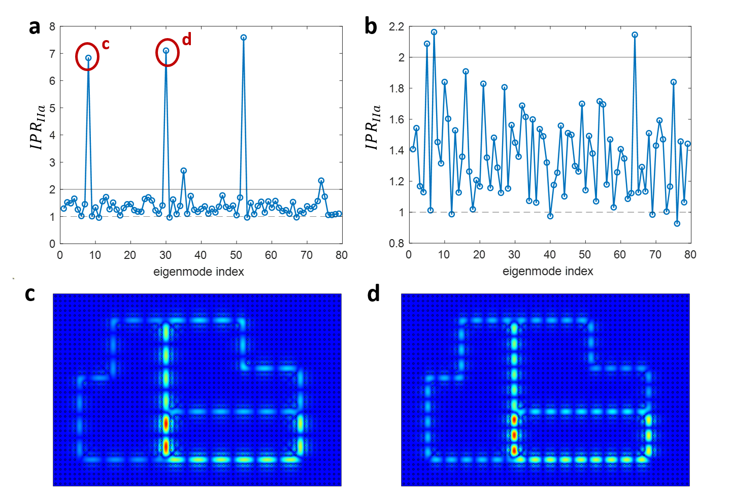
Figure 6: a. The inverse participation ratio (IPR) of the left side of the graph, computed based on method IIa. The simulated $|E_{z}|$ profile of the circled modes in a is shown in c (d). b. The IPR of the right side of the graph is computed based on method IIa. The solid and dashed lines in a. and b. refer to the RMT and the maximum ergodic limits, respectively.

Here we give a brief discussion on applying the inverse participation ratio (IPR) analysis to only a sub-region of the graph structure. Although the original definition of IPR is for the entire graph, we may apply the same computation in the context of subgraphs. Here we conduct subgraph IPR studies with bonds that only belong to the left half (one single loop) or the right half (two loops) of the PC graph shown in Fig. 6. The left half loop IPR is shown in Fig. 6 (a), computed based on method IIa. The IPRs computed with method IIb are not shown here. The majority of the eigenmodes have IPRs between the RMT (IPR = 2) and the maximum ergodic limits (IPR = 1). In the left half loop IPR test, we find three modes that have IPR values that reach the maximum localization limit (IPR = B, B = 7 for the left single loop). We show the eigenfunction profile of the two circled modes in Fig. 6 (c) and (d). These two modes indeed show a high degree of localization behavior, where the eigenfunction amplitude is mainly concentrated on one short bond. Fig. 6 (b) shows the IPR analysis of the right half graph. Here the modes with a higher degree of localization do not stand out in this subgraph IPR analysis. Thus we note that applying the IPR analysis to single loops can bring out the modes with a higher degree of localization.

References

- Hul et al. (2004) O. Hul, S. Bauch, P. Pakoński, N. Savytskyy, K. Życzkowski, and L. Sirko, Physical Review E 69, 056205 (2004).
- Martínez-Argüello et al. (2018) A. M. Martínez-Argüello, A. Rehemanjiang, M. Martínez-Mares, J. A. Méndez-Bermúdez, H.-J. Stöckmann, and U. Kuhl, Physical Review B 98, 075311 (2018).
- Rehemanjiang et al. (2020) A. Rehemanjiang, M. Richter, U. Kuhl, and H.-J. Stöckmann, Physical Review Letters 124, 116801 (2020).
- Lu et al. (2020) J. Lu, J. Che, X. Zhang, and B. Dietz, Physical Review E 102, 022309 (2020).
- Chen et al. (2020) L. Chen, T. Kottos, and S. M. Anlage, Nature Communications 11, 5826 (2020).
- Wu et al. (1998) D. H. Wu, J. S. A. Bridgewater, A. Gokirmak, and S. M. Anlage, Physical Review Letters 81, 2890 (1998).
- Dembowski et al. (2003) C. Dembowski, B. Dietz, H.-D. Gräf, A. Heine, F. Leyvraz, M. Miski-Oglu, A. Richter, and T. H. Seligman, Physical Review Letters 90, 014102 (2003).
- Dembowski et al. (2005) C. Dembowski, B. Dietz, T. Friedrich, H.-D. Gräf, H. L. Harney, A. Heine, M. Miski-Oglu, and A. Richter, Physical Review E 71, 046202 (2005).
- Hemmady et al. (2005) S. Hemmady, X. Zheng, E. Ott, T. M. Antonsen, and S. M. Anlage, Physical Review Letters 94, 014102 (2005).
- Kuhl et al. (2008) U. Kuhl, R. Höhmann, J. Main, and H.-J. Stöckmann, Physical Review Letters 100, 254101 (2008).
- Shinohara et al. (2010) S. Shinohara, T. Harayama, T. Fukushima, M. Hentschel, T. Sasaki, and E. E. Narimanov, Physical Review Letters 104, 163902 (2010).
- Dietz and Richter (2019) B. Dietz and A. Richter, Physica Scripta 94, 014002 (2019).
- Hemmady et al. (2012) S. Hemmady, T. M. Antonsen, E. Ott, and S. M. Anlage, IEEE Transactions on Electromagnetic Compatibility 54, 758 (2012).
- Xiao et al. (2018) B. Xiao, T. M. Antonsen, E. Ott, Z. B. Drikas, J. G. Gil, and S. M. Anlage, Physical Review E 97, 062220 (2018).
- Ma et al. (2019a) S. Ma, B. Xiao, R. Hong, B. Addissie, Z. Drikas, T. Antonsen, E. Ott, and S. Anlage, Acta Physica Polonica A 136, 757 (2019a).
- Ma et al. (2020a) S. Ma, B. Xiao, Z. Drikas, B. Addissie, R. Hong, T. M. Antonsen, E. Ott, and S. M. Anlage, Physical Review E 101, 022201 (2020a).
- Ma et al. (2020b) S. Ma, S. Phang, Z. Drikas, B. Addissie, R. Hong, V. Blakaj, G. Gradoni, G. Tanner, T. M. Antonsen, E. Ott, and S. M. Anlage, Physical Review Applied 14, 14022 (2020b).
- Frazier et al. (2020) B. W. Frazier, T. M. Antonsen, S. M. Anlage, and E. Ott, Physical Review Research 2, 043422 (2020).
- Mehta (2004) M. L. Mehta, Random matrices (Elsevier, 2004).
- Dietz et al. (2017a) B. Dietz, A. Heusler, K. H. Maier, A. Richter, and B. A. Brown, Physical Review Letters 118, 012501 (2017a).
- So et al. (1995) P. So, S. M. Anlage, E. Ott, and R. N. Oerter, Physical Review Letters 74, 2662 (1995).
- Bohigas et al. (1984) O. Bohigas, M. J. Giannoni, and C. Schmit, Physical Review Letters 52, 1 (1984).
- Zheng et al. (2006) X. Zheng, S. Hemmady, T. M. Antonsen, S. M. Anlage, and E. Ott, Physical Review E 73, 046208 (2006).
- Hart et al. (2009) J. A. Hart, T. M. Antonsen, and E. Ott, Physical Review E 80, 041109 (2009).
- Yeh et al. (2010) J.-H. Yeh, J. A. Hart, E. Bradshaw, T. M. Antonsen, E. Ott, and S. M. Anlage, Physical Review E 82, 041114 (2010).
- Li et al. (2015) X. Li, C. Meng, Y. Liu, E. Schamiloglu, and S. D. Hemmady, IEEE Transactions on Electromagnetic Compatibility 57, 448 (2015).
- Aurégan and Pagneux (2016) Y. Aurégan and V. Pagneux, Acta Acustica united with Acustica 102, 869 (2016).
- Zhou et al. (2019) M. Zhou, E. Ott, T. M. Antonsen, and S. M. Anlage, Chaos: An Interdisciplinary Journal of Nonlinear Science 29, 033113 (2019).
- Zhang et al. (2022) W. Zhang, X. Zhang, J. Che, J. Lu, M. Miski-Oglu, and B. Dietz, Physical Review E 106, 044209 (2022).
- Białous et al. (2016) M. Białous, V. Yunko, S. Bauch, M. Ławniczak, B. Dietz, and L. Sirko, Physical Review Letters 117, 144101 (2016).
- Dietz et al. (2017b) B. Dietz, V. Yunko, M. Białous, S. Bauch, M. Ławniczak, and L. Sirko, Physical Review E 95, 052202 (2017b).
- Che et al. (2021) J. Che, J. Lu, X. Zhang, B. Dietz, and G. Chai, Physical Review E 103, 042212 (2021).
- Johnson et al. (2001) S. Johnson, A. Mekis, S. Fan, and J. Joannopoulos, Computing in Science and Engineering 3, 38 (2001).
- Joannopoulos et al. (1997) J. D. Joannopoulos, P. R. Villeneuve, and S. Fan, Nature 386, 143 (1997).
- Joannopoulos et al. (2008) J. D. Joannopoulos, S. G. Johnson, J. N. Winn, and R. D. Meade, Photonic Crystals (Princeton University Press, 2008).
- Xiao et al. (2016) B. Xiao, K. Lai, Y. Yu, T. Ma, G. Shvets, and S. M. Anlage, Physical Review B 94, 195427 (2016).
- Lai et al. (2016) K. Lai, T. Ma, X. Bo, S. Anlage, and G. Shvets, Scientific Reports 6, 28453 (2016), 1601.01311 .
- Ma et al. (2019b) S. Ma, B. Xiao, Y. Yu, K. Lai, G. Shvets, and S. M. Anlage, Physical Review B 100, 085118 (2019b).
- Ma and Anlage (2020) S. Ma and S. M. Anlage, Applied Physics Letters 116, 250502 (2020).
- Liu et al. (2021) Y. G. N. Liu, P. S. Jung, M. Parto, D. N. Christodoulides, and M. Khajavikhan, Nature Physics 17, 704 (2021).
- Maimaiti et al. (2020) W. Maimaiti, B. Dietz, and A. Andreanov, Physical Review B 102, 214301 (2020).
- Zhang and Dietz (2021) W. Zhang and B. Dietz, Physical Review B 104, 064310 (2021).
- Reisner et al. (2021) M. Reisner, M. Bellec, U. Kuhl, and F. Mortessagne, Optical Materials Express 11, 629 (2021).
- Bittner et al. (2013) S. Bittner, B. Dietz, M. Miski-Oglu, A. Richter, C. Ripp, E. Sadurní, and W. P. Schleich, Physical Review E 87, 042912 (2013).
- Mekis et al. (1996) A. Mekis, J. C. Chen, I. Kurland, S. Fan, P. R. Villeneuve, and J. D. Joannopoulos, Physical Review Letters 77, 3787 (1996).
- Rehemanjiang et al. (2016) A. Rehemanjiang, M. Allgaier, C. H. Joyner, S. Müller, M. Sieber, U. Kuhl, and H.-J. Stöckmann, Physical Review Letters 117, 064101 (2016).
- Berry (1981) M. V. Berry, European Journal of Physics 2, 91 (1981).
- Kottos and Smilansky (1997) T. Kottos and U. Smilansky, Physical Review Letters 79, 4794 (1997).
- Kottos and Smilansky (1999) T. Kottos and U. Smilansky, Annals of Physics 274, 76 (1999).
- Casati et al. (1980) G. Casati, F. Valz-Gris, and I. Guarnieri, Lettere al Nuovo Cimento 28, 279 (1980).
- Haq et al. (1982) R. Haq, A. Pandey, and O. Bohigas, Physical Review Letters 48, 1086 (1982).
- Berry (1985) M. V. Berry, Proceedings of the Royal Society of London. A. Mathematical and Physical Sciences 400, 229 (1985).
- Atas et al. (2013) Y. Y. Atas, E. Bogomolny, O. Giraud, and G. Roux, Physical Review Letters 110, 084101 (2013).
- Kudrolli et al. (1995) A. Kudrolli, V. Kidambi, and S. Sridhar, Physical Review Letters 75, 822 (1995).
- Gokirmak et al. (1998) A. Gokirmak, D.-H. Wu, J. S. A. Bridgewater, and S. M. Anlage, Review of Scientific Instruments 69, 3410 (1998).
- Chung et al. (2000) S.-H. Chung, A. Gokirmak, D.-H. Wu, J. S. A. Bridgewater, E. Ott, T. M. Antonsen, and S. M. Anlage, Physical Review Letters 85, 2482 (2000).
- Kuhl et al. (2000) U. Kuhl, E. Persson, M. Barth, and H.-J. Stöckmann, The European Physical Journal B 17, 253 (2000).
- Hlushchuk et al. (2001) Y. Hlushchuk, L. Sirko, U. Kuhl, M. Barth, and H.-J. Stöckmann, Physical Review E 63, 046208 (2001).
- Kaplan (2001) L. Kaplan, Physical Review E 64, 036225 (2001).
- Alt et al. (1995) H. Alt, H. D. Gräf, H. L. Harney, R. Hofferbert, H. Lengeler, A. Richter, P. Schardt, and H. A. Weidenmüller, Physical Review Letters 74, 62 (1995).
- Hul et al. (2009) O. Hul, P. Šeba, and L. Sirko, Physical Review E 79, 066204 (2009).