Surrogate-based cross-correlation for particle image velocimetry

Abstract

This paper presents a novel surrogate-based cross-correlation (SBCC) framework to improve the correlation performance between two image signals. The basic idea behind the SBCC is that an optimized surrogate filter/image, supplanting one original image, will produce a more robust and more accurate correlation signal. The cross-correlation estimation of the SBCC is formularized with an objective function composed of surrogate loss and correlation consistency loss. The closed-form solution provides an efficient estimation. To our surprise, the SBCC framework could provide an alternative view to explain a set of generalized cross-correlation (GCC) methods and comprehend the meaning of parameters. With the help of our SBCC framework, we further propose four new specific cross-correlation methods, and provide some suggestions for improving existing GCC methods. A noticeable fact is that the SBCC could enhance the correlation robustness by incorporating other negative context images. Considering the sub-pixel accuracy and robustness requirement of particle image velocimetry (PIV), the contribution of each term in the objective function is investigated with particles’ images. Compared with the state-of-the-art baseline methods, the SBCC methods exhibit improved performance (accuracy and robustness) on the synthetic dataset and several challenging real experimental PIV cases.

I Introduction

Particle image velocimetry (PIV) is a non-intrusive technology for flow field measurement in experimental fluid dynamics[1, 2, 3]. PIV provides a quantitative vector field by analyzing the consecutive particle recordings. The particle images vary intensively with light illumination, particle diameters and distribution, recording settings, and the latent flow fields. Under such challenging circumstances, the accuracy of PIV measurement therefore could be significantly decreased. The specific problems are widely-recognized peak-locking[4, 5, 6] and outliers[7, 8, 9].

The mainstream analyzing methods can be cast into two categories: cross-correlation methods[10, 4, 11, 2, 12] and optical flow methods[13, 14, 15]. The vanilla cross-correlation provides the image similarity (dot product) as a function of the relative displacement, of which the calculation is computed efficiently in frequency domain via fast Fourier transform (FFT). With a concrete theoretical basis and consecutive modifications (detailed in Section II), the cross-correlation variants have achieved acceptable performance for most experimental or industrial measurements. Optical flow (OF) methods employ a preservation principle, namely that particle brightness attribute[15] (or other attributes[14]) is preserved during the motion, to estimate the image displacement. The risk of failure rises if the OF preservation principle breaks, which is common in a practical challenging measurement. Besides the mainstream methods, deep learning-based methods[8, 16, 17, 18] have been attracting researchers’ interest due to the powerful model capacity. The purported black box nature of neural networks is a barrier to adoption in PIV where interpretability is expected[19, 20]. In this paper, we focus on the cross-correlation methods, which are being employed by most practitioners[21, 22, 23, 24].

To enhance the correlation signal, improving the quality of the input image pair is a straightforward idea. a) The measurement environment (illumination, particles, time interval, etc) should be carefully set up to capture satisfactory recordings with less out-of-plane motion effect[2]. b) Image pre-processing techniques[25, 26, 27, 28] are adopted to improve image quality. c) Image offset [29, 30, 31] is employed to deal with large displacement, and thus reduces the in-plane loss of correlation. d) The image deformation scheme [32, 33] is adopted to meet the uniform displacement assumption of cross-correlation. All these methods achieve the correlation signal enhancement via replacing the original low-quality image with a processed surrogate. It thus might imply that the original image is not a good template for cross-correlation.

(a) Standard cross-correlation of PIV

(b) Correlation filter based object tracking

Figure 1: The comparison between cross-correlation for PIV (a) and correlation filter for object tracking (b).

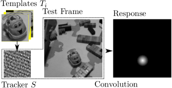
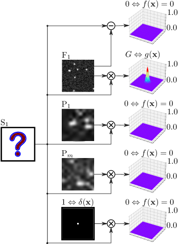
Correlation filters [34, 35, 36] have achieved competitive success in object tracking by online learning a discriminative linear filter/tracker from multiple image templates. The experiments exhibit that the learned filter outperforms the original image templates in robustness and accuracy [34, 37]. Different from the image pre-processing techniques, correlation filters find a filter/tracker that maximizes the convolution/tracking performance, as detailed in Section II. That is to say, the filter/tracker is designed with the best tracking performance. Fig. 1 shows the implementation difference between PIV and object tracking with correlation filters. The tracker $S$ produces appealing robust Gaussian-shaped response.

Our initial motivation is to directly incorporate correlation filters into PIV application, i.e., one interrogation image $F_{1}$ is replaced by a surrogate image/filter $S_{1}$ computed with the correlation filters. This combination method is named as correlation filter based cross-correlation (CFCC), as detailed in Section II. However, the CFCC method does not exhibit a satisfactory robustness (Section IV). Our insight is that the lack of positive templates is the cause of this problem. In contrast, a stable filter/tracker is achieved with multiple template images in the object tracking [34, 35].

As a remedy, we propose a surrogate-based cross-correlation (SBCC) framework, which combines a forward tracking with a backward tracking via correlation consistency objective. To gain robustness, our SBCC also considers the surrogate image performance on negative context images by carefully designing a surrogate loss. The surrogate images and cross-correlation response are jointly optimized under the overall SBCC objective. As a result, a closed-form solution is obtained. The main contributions of this work:

1. Inspired by correlation filter, the SBCC framework successfully combines cross-correlation and surrogate concept, resulting in novel cross-correlation methods.

2. To our surprise, several widely-used generalized cross-correlation methods are special cases of the closed-form solution of our SBCC. Therefore, the SBCC provides a surrogate view to explain the cross-correlation variants and comprehend the meaning of parameters.

3. The performance improvement of SBCC has been investigated on both synthetic and real PIV images.

The rest of this paper is arranged as follows. The related works with consistent mathematical notations are given in Section II. Section III describes our SBCC method from the problem modeling to optimization. And Section IV demonstrates the performance on synthetic datasets and real PIV images in comparison with baseline methods. Finally, the Section V ends the paper with several concluding comments.

II Related works

(a) SCC

(b) SCC with image pre-processing

(c) GCC

(d) CFCC

Figure 2: Different types of cross-correlation methods. The $\bigotimes$ denotes the standard cross-correlation in Fourier frequency domain (a). The SCC with image pre-processing in frequency domain (b). The generalized cross-correlation methods (c), the $\bigodot$ represents an element-wise multiplication. A correlation filter based cross-correlation method (d), the surrogate image $S_{1}$ is generated by minimizing the MOSSE objective $\mathcal{J}_{MOSSE}$ (solid blue arrow).

II-A Cross-correlation in the frequency domain

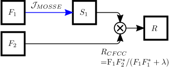
The cross-correlation response $r(\mathbf{x})$ of image pair $f_{1}(\mathbf{x})$, $f_{2}(\mathbf{x})$ contains the displacement information. Due to the Convolution Theorem, the computation of cross-correlation $r(\mathbf{x})$ becomes a fast element-wise multiplication in the Fourier frequency domain. That is to say, $R(\mathbf{\omega})=F_{1}(\mathbf{\omega})F^{*}_{2}(\mathbf{\omega})$, where $R(\omega),F_{1}(\omega),F_{2}(\omega)$ are the Fourier transform of $r(\mathbf{x})$, $f_{1}(\mathbf{x})$, $f_{2}(\mathbf{x})$ and the superscript $(^{*})$ denotes complex conjugation. Hereafter, we will simplify the notations ($F_{1}(\omega),F_{2}(\omega),...$) as ($F_{1},F_{2},...$) by omitting the frequency $\omega$. Due to its wide adoption in PIV estimation, this vanilla cross-correlation method will be referred to as the standard cross-correlation (SCC) method, as shown in Fig. 2 (a).

$$R_{SCC}=F_{1}F^{*}_{2}$$ (1)

The SCC has a satisfactory performance except for some challenging environments. The peak-locking effect increases as the particle image diameter is reduced [2], and SCC likely fails to predict the correct displacement under the strong background noisy circumstance [38]. A trick to improve the correlation result is to pre-process the image for SCC, demonstrated in Fig. 2 (b). Choosing a proper predefined frequency filter $H$ needs experts.

II-B Generalized cross-correlation

To enhance the correlation signal, the generalized cross-correlation (GCC) methods amend the SCC correlation $R_{SCC}$ with different frequency filters, i.e.,

$$R_{GCC}=\psi(F_{1},F_{2})F_{1}F_{2}^{*}$$ (2)

where $\psi(\cdot)$ denotes the modification operation (PHAT filter [39], SPOF filter [38], RPC filter [40], etc.). Several GCC instances are listed in Table. I. The filters of these GCC methods share a special type, $\psi(F_{1},F_{2})=\phi(|F_{1}F_{2}^{*}|)$, as demonstrated in Fig. 2 (c). Compared with the $R_{PRE}$ (image pre-processing), the $R_{GCC}$ can be viewed as a post-processing of $F_{1}F_{2}^{*}$.

TABLE I: Different cross-correlation methods.

Methods	Equations	Comments
SCC[2]	$R_{SCC}=F_{1}F_{2}^{*}$	$\psi(F_{1},F_{2})=1$
Pre-processing	$R_{PRE}=(HF_{1})(HF_{2})^{*}$	Filter $H$
PC[39]	$R_{PC}=\frac{F_{1}F_{2}^{*}}{|F_{1}F_{2}^{*}|}$	GCC method
SPOF[38]	$R_{SPOF}=\frac{F_{1}F_{2}^{*}}{\sqrt{|F_{1}F_{2}^{*}|}}$	GCC method
RPC[41, 40]	$R_{RPC}=\frac{GF_{1}F_{2}^{*}}{|F_{1}F_{2}^{*}|}$	GCC method
$\rho$-CSPC [42]	$R_{CSPC}=\frac{F_{1}F_{2}^{*}}{|F_{1}F_{2}^{*}|^{\rho}+\epsilon}$	GCC method
CFCC	$R_{CFCC}=\frac{GF_{1}F_{2}^{*}}{F_{1}F_{1}^{*}+\lambda}$	our method
SBCC_B1	$R_{B1}=\frac{2GF_{1}F_{2}^{*}}{F_{1}F_{1}^{*}+F_{2}F_{2}^{*}}$	our method
SBCC_B2	$R_{B2}=\frac{2GF_{1}F_{2}^{*}}{F_{1}F_{1}^{*}+F_{2}F_{2}^{*}+\lambda}$	our method
SBCC_B3	$R_{B3}=\frac{2(G+\mu G_{d}G_{d}^{*})F_{1}F_{2}^{*}}{F_{1}F_{1}^{*}+F_{2}F_{2}^{*}+2\mu G_{d}G_{d}^{*}}$	our method
SBCC	$R_{SBCC}=$ Eq.(12)	our method

In order to achieve unit amplitude (Dirac delta correlation response), phase correlation (PC) [39] method adopts a modified variant $R_{PC}$. The correlation peaks of $R_{PC}$ are very sharp, and thus peak-locking problem occurs. Wernet [38] proposed the symmetric phase-only filter (SPOF), which combines the SCC and PC method. In other words, the SPOF filter is a geometric mean of SCC filter $\psi(F_{1},F_{2})=1$ and PC filter $\psi(F_{1},F_{2})=(|F_{1}F_{2}^{*}|)^{-1}$. As a result, higher noisy frequencies are attenuated while also reducing the effects of additive background noise on the DPIV estimation. The GTPC [41] and robust phase correlation (RPC) [40] use an isotropic Gaussian transform filter, $G(\omega)\Leftrightarrow g(\mathbf{x})=exp(-\frac{\mathbf{x}^{2}}{2\sigma^{2}})$, in the spectral domain to transform the delta peak of PC into a Gaussian function. Our experiments demonstrate a vanilla RPC without zero-padding and advanced windowing techniques [40] produces more outliers than SCC method. The cause of occasional failure of RPC may be a numerical problem (the possibility of zero denominator). Researchers in [42, 43] suggest to add a positive value $\epsilon$ to the denominator, as $R_{CSPC}$. Totally speaking, these GCC filters reflect the successful experience of practitioners and researchers. However, it is not easy to comprehend the special choice of $\epsilon$ [42, 43], which seems to be a simple trick to prevent the denominator from being zero. And it is still an open question whether it could have other GCC filters $\psi(\cdot)$.

II-C Correlation filters and CFCC

Figure 3: A schematic diagram to understand the objective of MOSSE, $\mathcal{J}_{MOSSE}$. The $\bigotimes$ denotes the standard cross-correlation.

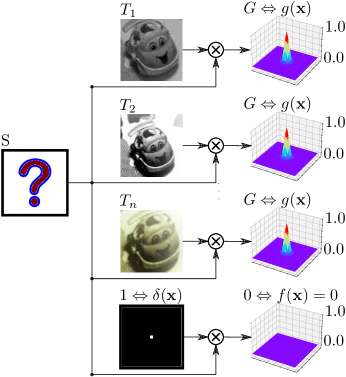
The correlation filter can be derived either from an objective function specifically formularized in the Fourier domain [34] or from ridge regression and circulant matrices [35, 36]. Slightly different from [34, 35], we provide our understanding of correlation filter as following. As shown in Fig. 3, given a set of aligned template images $T_{i},i\in\{1,2,...,n\}$, the MOSSE method [34, 35] finds a surrogate filter/tracker $S$ that produces the best tracking performance, i.e., the cross-correlation response $r_{i}(\textbf{x})=\mathcal{F}^{-1}(T_{i}S^{*})$ is encouraged to be an isotropic Gaussian-shaped response $g(\mathbf{x})$, where $\mathcal{F}^{-1}(\cdot)$ denotes inverse fourier transform. In addition, a regularization term $|S|^{2}$ is employed to avoid the over fitting and gains the stability, similar to Wiener filtering or ridge regression [35].

$$\begin{split}\hat{S}&=\arg\mathop{\min}_{S}\mathcal{J}_{MOSSE}(S)\\ \end{split}$$ (3)

with the minimum output sum of squared error (MOSSE),

$$\begin{split}\mathcal{J}_{MOSSE}(S)=\mathop{\Sigma}_{i=1}^{n}|G-T_{i}S^{*}|^{2}+\lambda|S|^{2}\end{split}$$ (4)

where $\lambda>0$ controls the amount of regularization, and it is recommended to be $0.1$ [34]. The $n$ is the number of positive templates, and $G$ denotes the Fourier transform of a Gaussian function $g(\mathbf{x})$. A closed-form solution of MOSSE is arrived:

$$\hat{S}^{*}=\frac{\Sigma_{i}GT_{i}^{*}}{\Sigma_{i}T_{i}T_{i}^{*}+\lambda}$$ (5)

The $\lambda$ prevents the denominator from being zero.

Our observation is that the regularization term of Eq.(4), $|S|^{2}=|0-1\cdot S^{*}|^{2}$, could be regarded as a special term for a negative template (delta function, $1\Leftrightarrow\delta(\mathbf{x})$), as demonstrated in Fig. 3. That is to say, the MOSSE filter also expects the cross-correlation between $S$ and a negative Dirac delta function to be zero. Now, it is clear that the parameter $\lambda$ controls the importance for this negative template response.

A new generalized cross-correlation method, acronymed CFCC, is proposed by replacing one image $F_{1}$ with the surrogate filter $(\frac{GF_{1}}{F_{1}F_{1}^{*}+\lambda})$ of correlation filter. In other words, one original image is pre-processed with MOSSE filter, and the second original image does not change.

$$R_{CFCC}=\frac{GF_{1}F_{2}^{*}}{F_{1}F_{1}^{*}+\lambda}$$ (6)

The CFCC method, a direct combination of correlation filter and cross-correlation, does provide an improved shape of cross-correlation peak. However it does not achieve satisfactory results due to a large number of outliers (Section IV).

III Surrogate-based cross-correlation

Figure 4: Our surrogate-based cross-correlation framework. The surrogate images $S_{1},S_{2}$ and correlation response $R$ are jointly optimized with surrogate objective $\mathcal{J}_{surr}$ and correlation consistency objective $\mathcal{J}_{corr}$ (blue dash arrows). The $\bigotimes$ denotes the standard cross-correlation. The $R_{f}$ and $R_{b}$ represent the correlation response with forward surrogate ($S_{1}$) and backward surrogate ($S_{2}$) respectively.

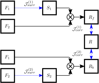
As shown in Fig. 4, the proposed SBCC framework utilizes a bidirectional surrogate structure to achieve an enhanced correlation response $R$. A surrogate filter/image ($S_{1}$ or $S_{2}$) is assumed to have a better cross-correlation response under a well-designed surrogate objective $\mathcal{J}_{surr}$, which considers the tracking performance as well as robustness. The forward correlation response $R_{f}$ (with surrogate $S_{1}$) and backward response $R_{b}$ (with surrogate $S_{2}$) are combined via correlation consistency objective $\mathcal{J}_{corr}$. Because the variables $S_{1}$, $S_{2}$ and $R$ are coupled in this framework, the problem is formularized as a joint optimization with an objective function $\mathcal{J}_{SBCC}$.

$$\begin{split}\hat{R},\hat{S}_{1},\hat{S}_{2}&=\mathop{\arg\min}_{R,S_{1},S_{2}}\mathcal{J}_{SBCC}(R,S_{1},S_{2};F_{1},F_{2})\\ \end{split}$$ (7)

with

$$\begin{split}\mathcal{J}_{SBCC}&(R,S_{1},S_{2};F_{1},F_{2})\\ &=\underbrace{\mathcal{J}_{surr}^{(1)}(S_{1};F_{1})+\mathcal{J}_{surr}^{(2)}(S_{2};F_{2})}_{\textrm{surrogate objective}}\\ &\quad+\underbrace{\mathcal{J}_{corr}^{(1)}(R_{f},R)+\mathcal{J}_{corr}^{(2)}(R_{b},R)}_{\textrm{correlation consistency objective}}\\ \end{split}$$ (8)

where $R_{f}=S_{1}F_{2}^{*},R_{b}=F_{1}S_{2}^{*}$ are the forward correlation response and backward correlation response.

In the remainder of this section, we first describe the specific surrogate objective function and correlation consistency objective function of SBCC, and then proceed to detail the optimization and explain the connections between our SBCC framework and several classical GCC methods.

III-A Surrogate objective and correlation consistency objective

Figure 5: A schematic diagram to understand the surrogate objective of SBCC, $\mathcal{J}_{surr}$. The $P_{1},P_{2},...,P_{m}$ denote negative context images. The $\bigotimes$ denotes the standard cross-correlation. The $\ominus$ operation computes the difference between $F_{1}$ and $S_{1}$.

It is a challenge to bring the surrogate concept to practical cross-correlation for PIV application, because of the robust problem of the MOSSE filter/tracker under one positive PIV template circumstance. To gain the stability of surrogate filter, we construct a well-designed surrogate objective, which makes full use of the positive template and considers other negative context images. The negative samples are proved to be useful for representation learning [44, 45]. As shown in Fig. 5, our surrogate objective $\mathcal{J}_{surr}$ is firstly given before a detail explanation.

$$\begin{split}\mathcal{J}_{surr}(S;F)&=\underbrace{|G-FS^{*}|^{2}+\lambda|0-1\cdot S^{*}|^{2}}_{\textrm{MOSSE term}}\\ &\quad+\underbrace{\mu|G_{d}F-G_{d}S|^{2}}_{\textrm{difference term}}\\ &\quad+\underbrace{\nu\frac{1}{m}\mathop{\Sigma}_{i=1}^{m}|0-P_{i}S^{*}|^{2}}_{\textrm{negative context term}}\\ &=|G-FS^{*}|^{2}+\lambda|S|^{2}\\ &\quad+\mu|G_{d}F-G_{d}S|^{2}+\nu\frac{1}{m}\mathop{\Sigma}_{i=1}^{m}|P_{i}S^{*}|^{2}\\ \end{split}$$ (9)

where $P_{i},i\in\{1,2,...,m\}$ are the negative context templates. The $G$ and $G_{d}$ denote the Fourier transform of Gaussian functions $g(\mathbf{x})$ and $g_{d}(\mathbf{x})$. The $\{\lambda,\mu,\nu\}$ are coefficients for regularization, difference term, and context images term. The MOSSE term $\mathcal{J}_{MOSSE}$ is preserved to encourage a Gaussian-shaped correlation peak. The second difference term is based on the observation that the original image $F$ is often an acceptable tracker for PIV, thus the surrogate $S$ is encouraged to be close to the original image $F$. Most outliers occur when the images have similar image background or other noisy pattern. Reducing the filter’s response to the background/noise could decrease the number of outliers. Recall that the regularization term $|S|^{2}$, the negative context term encourages the filter $S$ also produce zero response to the context images. We choose the other negative interrogation windows as the context images. Compared to the $\delta(\mathbf{x})$, the context images are more likely to have a similar noisy pattern with $F_{2}$.

Different from the object tracking task, PIV could treat the paired images as templates to each other. Our SBCC framework (Fig. 4) models it as forward and backward correlation. To obtain a consistency correlation result, a consistency objective encourages the consistence between $R_{f}$ and $R_{b}$.

$$\begin{split}\mathcal{J}_{corr}(R)&=\mathcal{J}^{(1)}_{corr}(R_{f},R)+\mathcal{J}^{(2)}_{corr}(R_{b},R)\\ &=|R-R_{f}|^{2}+|R-R_{b}|^{2}\\ &=|R-S_{1}F_{2}^{*}|^{2}+|R-F_{1}S_{2}^{*}|^{2}\\ \end{split}$$ (10)

where $R$ is the final cross-correlation response of SBCC.

III-B Optimization of our SBCC objective function

Take the surrogate objective Eq. 9 and correlation consistency objective Eq. 10 back into the problem, Eq. (LABEL:eq_objective_SBCC). The specific objective function of SBCC is arrived,

$$\begin{split}\mathcal{J}_{SBCC}&(R,S_{1},S_{2};F_{1},F_{2})\\ &=|G-F_{1}S_{1}^{*}|^{2}+\lambda|S_{1}|^{2}\\ &\quad+\mu|G_{d}F_{1}-G_{d}S_{1}|^{2}+\nu\frac{1}{m}\mathop{\Sigma}_{i=1}^{m}|P_{i}S_{1}^{*}|^{2}\\ &\quad+|G-F_{2}S_{2}^{*}|^{2}+\lambda|S_{2}|^{2}\\ &\quad+\mu|G_{d}F_{2}-G_{d}S_{2}|^{2}+\nu\frac{1}{m}\mathop{\Sigma}_{i=1}^{m}|P_{i}S_{2}^{*}|^{2}\\ &\quad+|R-S_{1}F_{2}^{*}|^{2}+|R-F_{1}S_{2}^{*}|^{2}\\ \end{split}$$ (11)

This function is the sum of several squared errors between the actual cross-correlation responses and the desired responses. The $\{\lambda,\mu,\nu\}$ controls the relative importance of responses for $\delta(\mathbf{x})$, $G_{d}$ and negative context images.

The optimization of $\mathcal{J}_{SBCC}$ is almost identical to the optimization problems in [34, 35]. The difference is that SBCC objective is a function with three variables. A closed-form solution for SBCC is found by setting the partials to zero, as detailed in Appendix. A.

$$\begin{split}R_{SBCC}&=\hat{R}\\ &=\frac{2(G+\mu G_{d}G_{d}^{*})F_{1}F_{2}^{*}}{F_{1}F_{1}^{*}+F_{2}F_{2}^{*}+2\lambda+2\mu G_{d}G_{d}^{*}+2\nu Q}\\ \end{split}$$ (12)

$$\begin{split}\hat{S}_{1}&=\frac{F_{2}\hat{R}+GF_{1}+\mu G_{d}G_{d}^{*}F_{1}}{F_{1}F_{1}^{*}+F_{2}F_{2}^{*}+\lambda+\mu G_{d}G_{d}^{*}+\nu Q}\\ \hat{S}_{2}^{*}&=\frac{F_{1}^{*}\hat{R}+GF_{2}^{*}+\mu G_{d}G_{d}^{*}F_{2}^{*}}{F_{1}F_{1}^{*}+F_{2}F_{2}^{*}+\lambda+\mu G_{d}G_{d}^{*}+\nu Q}\\ \end{split}$$ (13)

Where $Q=\frac{1}{m}\Sigma_{i=1}^{m}P_{i}P_{i}^{*}$ is the average Fourier power spectrum of negative context images. The cross-correlation response, $R_{SBCC}$, incorporates this $Q$ component, resulting in a robustness correlation by considering the noisy background in these context images. The terms in $R_{SBCC}($Eq. (12)) have clear interpretation. The numerator is the cross-correlation between $F_{1}$ and $F_{2}$ with a Gaussian mixture filter ($G+\mu G_{d}G_{d}^{*}$), and the denominator is the power spectrum sum of $F_{1}$, $F_{2}$, $\delta(\mathbf{x})$, $g_{d}(\mathbf{x})$, and negative context images. Note that the surrogate $\hat{S}_{1}$ depends on both $F_{1}$ and $F_{2}$.

III-C Explain the GCC methods in SBCC view

Each term of the objective function $\mathcal{J}_{SBCC}$ has a clear meaning, and the solution $R_{SBCC}$ has good interpretation as well. According to our SBCC solution, a set of GCC methods are special configuration with additional constraint. As a result, our SBCC framework connects the existing GCC methods with a new surrogate interpretation.

At first, we review the GCC equations and our SBCC solution mathematically. The SCC method pays infinite attention to the difference term ($\mu\rightarrow\infty$), that is

$$R_{SCC}=\lim_{\mu\rightarrow\infty}R_{SBCC}$$ (14)

Now we consider a useful equation.

$$F_{1}F_{1}^{*}+F_{2}F_{2}^{*}=(|F_{1}|-|F_{2}|)^{2}+2|F_{1}F_{2}^{*}|\geq 2|F_{1}F_{2}^{*}|$$ (15)

Thus, the mathematical representation of PC, RPC, 1-CSPC become special SBCC cases with an additional constraint $|F_{1}|=|F_{2}|$. That says,

$$\begin{split}R_{PC}\ \ &=R_{SBCC}|_{\mu=0,\nu=0,G=1,\lambda=0,|F_{1}|=|F_{2}|}\\ R_{1-CSPC}&=R_{SBCC}|_{\mu=0,\nu=0,G=1,|F_{1}|=|F_{2}|}\\ R_{RPC}&=R_{SBCC}|_{\mu=0,\nu=0,G\Leftrightarrow g(x),\lambda=0,|F_{1}|=|F_{2}|}\\ \end{split}$$ (16)

The condition $|F_{1}|^{2}+|F_{2}|^{2}+\lambda=2\sqrt{|F_{1}F_{2}^{*}|}$ of SPOF is beyond our understanding. However, the SPOF can be treated as an ensemble correlation [46] due to the Eq. (17).

$$R_{SPOF}R_{SPOF}=R_{SCC}R_{PC}$$ (17)

It might imply that multiple SBCC frameworks may provide a complex surrogate explanation to SPOF and $\rho-$CSPC.

TABLE II: Comparison of different cross-correlation methods with SBCC framework.

Methods	$\lambda$	$\mu$	$\nu$	$G$	$|F_{1}|=|F_{2}|$	Negative images	Key comments
SCC	-	$\infty$	-	-	-	-	surrogate is the original image.
PC	0	0	0	$1\Leftrightarrow\delta(\mathbf{x})$	$\checkmark$	$\times$	encourage a $\delta$ response.
1-CSPC	$0<\lambda<1$	0	0	$1\Leftrightarrow\delta(\mathbf{x})$	$\checkmark$	$\delta(\mathbf{x})$	-
SPOF	$\lambda>0$	0	0	$1\Leftrightarrow\delta(\mathbf{x})$	$\checkmark$	$\delta(\mathbf{x})$	ensemble correlation
RPC	0	0	0	$G\Leftrightarrow g(\mathbf{x})$	$\checkmark$	$\times$	encourage Gaussian response.
SBCC_B1	0	0	0	$G\Leftrightarrow g(\mathbf{x})$	$\times$	$\times$	discard the constraint, $|F_{1}|=|F_{2}|$.
SBCC_B2	0.1	0	0	$G\Leftrightarrow g(\mathbf{x})$	$\times$	$\delta(\mathbf{x})$	-
SBCC_B3	0	1	0	$G\Leftrightarrow g(\mathbf{x})$	$\times$	$\times$	add difference term.
SBCC	0	1	10	$G\Leftrightarrow g(\mathbf{x})$	$\times$	$P_{i},i\in\{1,...,m\}$	negative context images.

To this end, Table. II summarizes the different cross-correlation methods in our SBCC view. The surrogate of SCC is the original image, $S_{1}=F_{1}$. The PC method encourages a Dirac delta response by setting $G=1$, whereas the RPC method encourages a Gaussian response by setting $G\Leftrightarrow g(\mathbf{x})$. The 1-CSPC method and SPOF method improve the PC with a negative image $\delta(\mathbf{x})$, adding $\lambda$ to the denominator. The PC, 1-CSPC and RPC methods all employ a constraint $|F_{1}|=|F_{2}|$. This constraint is automatically satisfied for the high quality image. However, it is easily broke due to the unknown image background or noise. Note that none of the existing GCC methods consider the negative context images.

IV Experimental investigation

In this section, the correlation responses are firstly visualized with various particle images. And then, the standard accuracy experiments are conducted with uniform flows and non-uniform flows. At last, three real PIV cases are tested.

To evaluate the performance, we compare our SBCC($\lambda=10^{-5},\mu=1.0,\nu=10.0$) and CFCC(Eq. (6)) against SCC [2], SPOF [38], RPC [40]. We also tested three variants of SBCC with different parameter configuration: SBCC_B1($\lambda=10^{-5},\mu=0.0,\nu=0.0$), SBCC_B2($\lambda=0.1,\mu=0.0,\nu=0.0$) and SBCC_B3($\lambda=10^{-5},\mu=1.0,\nu=0.0$), as shown in Table. I and Table. II. The $\lambda$ is set to $10^{-5}$ for numerical stability in implementation. Without specific annotation, the interrogation window is all set to $32\times 32$ pixel², and the default step size is 16 pixel.

• Comparing the RPC and SBCC_B1, we can clarify the contribution of discarding the constraint $(|F_{1}|=|F_{2}|)$.

• Comparing the SBCC_B2 and SBCC_B1, the contribution of the special negative image $(\delta(\mathbf{x}))$ is emphasized.

• Comparing the SBCC_B3 and SBCC_B1, we can understand the contribution of the difference term.

• Comparing the SBCC and SBCC_B3, we can understand the contribution of the negative context images.

IV-A Correlation coefficients map analysis

Figure 6: The correlation responses on synthetic particle images. The $d_{p}$ denotes the particles diameter in pixel. Best viewed in color.

Figure 7: The correlation responses on turbulent jet images [7]. The $F_{1}$ and $F_{2}$ are the interrogation images at the center (white square). Best viewed in color.

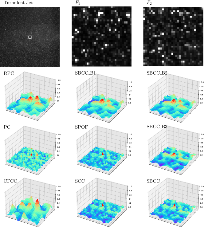
Fig. 6 gives the correlation responses for synthetic particle images under an arbitrary uniform flow $(u=5.25$ pixel, $v=0.0$ pixel). All the methods achieve strong correct peak signals ($>0.4$). The responses of PC and SPOF have sharp peaks for different particle diameters. The response shape of SCC strongly depends on the particle diameters. In contrast, the CFCC, RPC, SBCC_B1, and SBCC_B2 share similar Gaussian-shaped peak responses regardless the particles diameter configuration. This observation verified our initial assumption, the surrogate images could achieve a desired Gaussian-shaped correlation response on such simulated images.

The real experimental cases are more complicated, with unwanted noise/backgrounds or out-of-plane motion. Fig. 7 demonstrates the correlation responses for an experimental turbulent jet flow [7]. The maximum correlation coefficients are small ($\approx 0.2$) due to the strong out-of-plane turbulent motion. The RPC and CFCC have wrong peak locations, while other methods obtain correct peaks. The shape of these peaks determine the corresponding accuracy. The sharp peaks (PC, SPOF, SCC) implies risks of peak-locking, while the Gaussian-shaped peaks (SBCC_B1, SBCC_B2, SBCC_B3, SBCC) are more likely to achieve accurate estimations.

It is interesting to compare RPC and SBCC_B1. For the ideal synthetic cases, the constraint $|F_{1}|=|F_{2}|$ is almost satisfied, RPC and SBCC_B1 have almost identical performance. Our SBCC_B1 achieves a better correlation response over the Turbulent Jet case because the SBCC_B1 does not require the strict constraint ($|F_{1}|=|F_{2}|$) of RPC. There is no significant difference between the responses of SBCC_B1 and SBCC_B2, because the special $\delta(\mathbf{x})$ noise is not likely to occur in these cases. Compared with SBCC_B1, our SBCC_B3 and SBCC reduce the second peak’s coefficients. Our SBCC methods thus are more likely to achieve robust performance.

IV-B Assessment on uniform flow

(a) $d_{p}=0.6$ pixel

(b) $d_{p}=2.2$ pixel

(c) $d_{p}=4.0$ pixel

Figure 8: Measurement uncertainty as a function of displacement and various particle diameters $d_{p}$. (Simulation density $C_{p}=0.02ppp$, particles per pixel.)

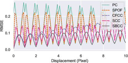
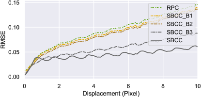
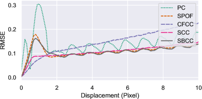
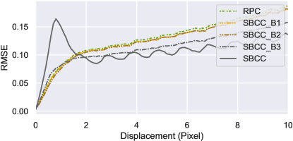
The Monte Carlo simulation is widely adopted in the assessment of the measurement uncertainty of PIV [2, 8]. The test particle images (size: $256\times 256$) are simulated under uniform flow patterns. For a given displacement, the root mean square error (RMSE) is computed from 100 runs.

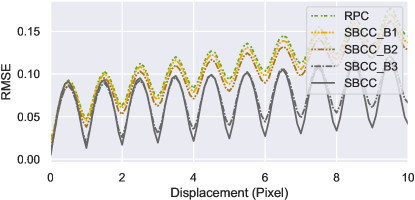
Fig. 8 shows the simulation results for the RMSE as a function of the displacement. The performance of SCC agrees well with the reported results of [2, 8], and the peak-locking is introduced when the particle diameter is too small. The PC method has the largest error on average, and demonstrates strong peak-locking even when the particle diameter reaches $4.0$ pixel. Our explanation is that PC method only encourages a Dirac delta response. The CFCC baseline demonstrates excellent performance for displacements less than $1.0$ pixel, because the MOSSE filter is designed for a better tracking. However, the unstable tracker from one positive template does not perform well for larger displacement.

The interesting step-by-step improvements of SBCC method are observed. That says, the SBCC_B1 performs better than RPC, the SBCC_B2 performs better than SBCC_B1, the SBCC_B3 performs better than SBCC_B2, and the SBCC performs better than SBCC_B3. More interestingly, these performance improvements can be interpreted with our SBCC framework. The RPC method implicitly has a strict constraint $(|F_{1}|=|F_{2}|)$ that causes an accuracy degradation. Employing a negative delta image (SBCC_B2), a difference term (SBCC_B3), and negative context images (SBCC) are contributed to the performance improvement. Considering both the tracking performance and robustness, our SBCC method thus achieves a competitive accuracy in comparison with the PC, SPOF, RPC, and SCC methods.

IV-C Assessment on complex fluids flow

TABLE III: The RMSE results on Cai’s dataset[18]. The best in bold.

Case	PC	SPOF	CFCC	SCC	RPC	SBCC_B1	SBCC_B2	SBCC_B3	SBCC
Uniform	0.208	0.070	0.112	0.059	0.095	0.090	0.087	0.065	0.061
Back-step	0.306	0.135	0.142	0.117	0.134	0.130	0.128	0.115	0.121
Channel	0.253	0.166	0.160	0.157	0.161	0.160	0.158	0.156	0.162
Cylinder	0.429	0.359	0.362	0.353	0.360	0.360	0.360	0.354	0.351
SQG	1.263	0.677	0.682	0.607	0.581	0.570	0.569	0.538	0.610
DNS-turbulence	1.488	0.815	0.843	0.687	0.666	0.660	0.636	0.613	0.715

TABLE IV: The outlier percentage on Cai’s dataset[18]. The best (except 0.00%) in Bold.

Case	PC	SPOF	CFCC	SCC	RPC	SBCC_B1	SBCC_B2	SBCC_B3	SBCC
Uniform	0.11%	0.00%	0.01%	0.00%	0.00%	0.00%	0.00%	0.00%	0.00%
Back-step	0.07%	0.00%	0.00%	0.00%	0.00%	0.00%	0.00%	0.00%	0.00%
Channel	0.00%	0.00%	0.00%	0.00%	0.00%	0.00%	0.00%	0.00%	0.00%
Cylinder	0.06%	0.04%	0.01%	0.02%	0.01%	0.01%	0.01%	0.01%	0.01%
SQG	2.39%	0.54%	0.48%	0.35%	0.28%	0.19%	0.20%	0.23%	0.37%
DNS-turbulence	3.66%	1.30%	1.17%	0.93%	0.73%	0.65%	0.64%	0.63%	1.02%

Considering the complexity of fluids flow, another synthetic dataset [18, 17, 47] is adopted to evaluate the performance under complex flow patterns. The flow fields for test are from either computational fluid dynamics (CFD) simulation or the John Hopkins Turbulence Database (JHTDB). It contains six flow types, i.e., uniform flow, backward stepping flow, flow over a circular cylinder, homogeneous isotropic turbulent flow, SQG sea surface flow, and channel flow provided by JHTDB. Herein, 200 image pairs for each type were randomly chose to evaluate the performance of cross-correlation methods.

Table. III shows the RMSE results and Table. IV provides the outlier percentage. As the complexity of flow field increases, the measurement error and outliers also increases [32, 33]. The SBCC_B3 achieves four best accuracy out of six test sets, it means that our SBCC framework also works well for non-uniform flows. Because these synthetic test images are noise-free, the SBCC does not exhibit performance improvement. Besides, the results of these methods are reliable as the low level of outlier ratio $(<1\%)$.

IV-D Assessment on laboratory recordings

TABLE V: The outlier counts on the real experimental PIV images. The best in bold.

Test Cases	PC	SPOF	CFCC	SCC	RPC	SBCC_B1	SBCC_B2	SBCC_B3	SBCC
Wall Jet Flow [48]	8	1	16	3	5	3	3	3	2
Rotating Flow [24]	11	5	123	8	64	58	59	22	5
Turbulent Jet Flow [7]	290	144	421	98	263	227	203	87	60

Figure 9: Vectors calculated from real PIV images represent a wall jet flow [48]. The color corresponds to velocity magnitude. Best viewed in color.

Figure 10: Vectors calculated from real PIV images represent a rotating flow [24]. The color corresponds to velocity magnitude. Best viewed in color.

Figure 11: Vectors calculated from real PIV images represent a turbulent jet flow [7]. The color corresponds to velocity magnitude. Best viewed in color.

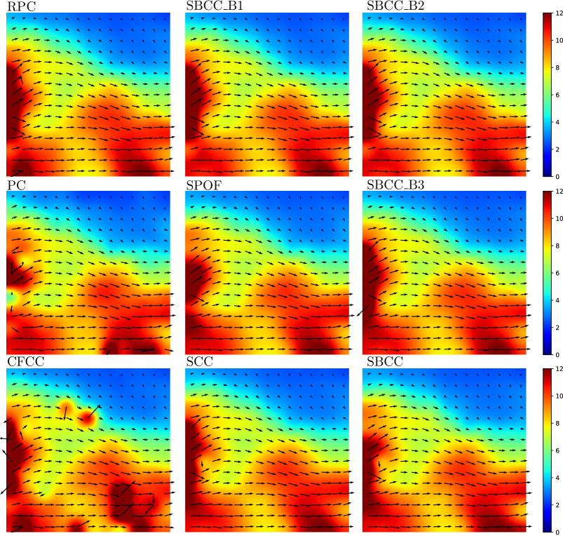
Finally, we test on three public available PIV image pairs. The first case records of a turbulent jet impinging on the wall [48]. The second PIV case records a liquid column rotating at steady uniform angular velocity (PIV Challenge 2014, Case F) [24]. The third image pair reflects a turbulent jet flow, provided by Westerweel and Scarano [49, 7]. These flows have small-scale turbulent structures with large displacement ($\approx 10$ pixel), and the images have non-uniform illumination, noise background and out-of-plane effects. Thus, these cases are considered as challenging test examples. Fig. 9, 10 and 11 provide the original vector field results, computed with different cross-correlation methods without any post-processing operation. The pseudo-color backgrounds represent the vector magnitudes. Table. V counts the number of outliers with a threshold method $|\mathbf{u}-\mathbf{u}_{ref}|^{2}>4.0$, where the reference vector $\mathbf{u}_{ref}$ is computed with the three-pass window deformation iterative method (WIDIM) [32, 8]. The vector $\mathbf{u}$ is labeled as an outlier if it is far from the corresponding reference. The outlier counts agree well with the visual inspection results.

As shown in Fig. 9, 10 and 11, all methods output similar flow structures. Due to the unknown truth, we can’t tell the exact accuracy for each method. But the PC method exhibits a distinguishable peak-locking effect in Fig. 10. The CFCC baseline only works well in the ideal conditions of small displacement ($<4$ pixel) and good-quality image, and it has massive outliers for all three cases. Our SBCC method merely produces 2 outliers for the Wall Jet, 5 outliers for the Rotating case, and 60 outliers for the Turbulent Jet. The SBCC therefore exhibits the best robustness. Besides, the classical SCC and SPOF achieve satisfactory performance due to a small quantity of outliers. Interestingly, the number $\mathbf{N}$ of outliers almost satisfy the following rule, $\mathbf{N}_{RPC}>\mathbf{N}_{SBCC\_B1}\approx\mathbf{N}_{SBCC\_B2}\geq\mathbf{N}_{SBCC\_B3}>\mathbf{N}_{SBCC}$. It reveals the individual contribution of the SBCC objective terms. With a implicit constraint $|F_{1}|=|F_{2}|$, the RPC has more outliers than that of SBCC_B1. The negative delta image $\delta(\mathbf{x})$ does not improve the robustness of SBCC_B2, because it is hardly possible to meet a delta image $\delta(\mathbf{x})$ in reality. The difference term (SBCC_B3) and negative context images (SBCC) can reduce the outliers significantly.

V Conclusion

A SBCC framework is proposed to improve the cross-correlation performance via surrogate images. With the help of this framework, several new cross-correlation methods (SBCC_B1, SBCC_B2, SBCC_B3, and SBCC) are introduced, as a result of different parameter settings. Based on the closed-form solution, this framework provides an surrogate-based explanation for a set of cross-correlation methods, including the SCC, PC, SPOF, RPC, and $1-$CSPC method. And the PC, RPC and $1-$CSPC methods are found to have an implicit constraint $(|F_{1}|=|F_{2}|)$ that leads to a performance degradation. The CFCC and SBCC methods demonstrate the desired Gaussian-shaped correlation response, which is encouraged by the objective function. Through the experimental investigation with PIV images, there is an interesting step-by-step performance improvement for PC, RPC, SBCC_B1, SBCC_B2, SBCC_B3, and SBCC. These gradual changes confirm the contribution of each term in our SBCC objective function. An interesting finding is that employing negative context images in SBCC is beneficial for correlation robustness. A special negative image $(\delta(\mathbf{x}))$ only has a limited positive effect. Moving forward, we plan to apply SBCC beyond PIV to other tasks including one-dimensional time series[50], digital image correlation[51], object tracking[52], visual servo[53], acoustic imaging[54], etc.

Appendix A Minimizing the SBCC objective

Here we provide a more detailed derivation of SBCC optimization following the previous works [34]. The minimization problem of SBCC is set up as:

$$\begin{split}\hat{R},\hat{S}_{1},\hat{S}_{2}=\arg\mathop{\min}_{R,S_{1},S_{2}}\mathcal{J}_{SBCC}(R,S_{1},S_{2};F_{1},F_{2})\end{split}$$ (18)

Because every terms of $\mathcal{J}_{SBCC}(\cdot)$ are element-wise operation, each element can be optimized independently. That says,

$$\begin{split}\hat{R}&{}_{\omega},\hat{S}_{1,\omega},\hat{S}_{2,\omega}\\ &=\mathop{\arg\min}_{R_{\omega},S_{1,\omega},S_{2,\omega}}\mathcal{J}_{SBCC,\omega}(R_{\omega},S_{1,\omega},S_{2,\omega})\end{split}$$ (19)

the subscript $\omega$ index the elements. With the element objective,

$$\begin{split}\mathcal{J}&{}_{SBCC,\omega}(R_{\omega},S_{1,\omega},S_{2,\omega})\\ &=|G_{\omega}-F_{1,\omega}S_{1,\omega}^{*}|^{2}+\lambda|S_{1,\omega}|^{2}\\ &\quad+\mu|G_{d,\omega}F_{1,\omega}-G_{d,\omega}S_{1,\omega}|^{2}\\ &\quad+\nu\frac{1}{m}\mathop{\Sigma}_{i=1}^{m}|P_{i,\omega}S_{1,\omega}^{*}|^{2}\\ &\quad+|G_{\omega}-F_{2,\omega}S_{2,\omega}^{*}|^{2}+\lambda|S_{2,\omega}|^{2}\\ &\quad+\mu|G_{d,\omega}F_{2,\omega}-G_{d,\omega}S_{2,\omega}|^{2}\\ &\quad+\nu\frac{1}{m}\mathop{\Sigma}_{i=1}^{m}|P_{i,\omega}S_{2,\omega}^{*}|^{2}\\ &\quad+|R_{\omega}-S_{1,\omega}F_{2,\omega}^{*}|^{2}+|R_{\omega}-F_{1,\omega}S_{2,\omega}^{*}|^{2}\\ \end{split}$$ (20)

This objective $\mathcal{J}_{SBCC,\omega}(\cdot)$ is a real value function of complex variables ($R_{\omega},S_{1,\omega},S_{2,\omega}$). This type of optimization problem has a closed form solution [34] by setting the following partial derivatives to zero.

$$\begin{split}\frac{\partial\mathcal{J}_{SBCC,\omega}}{\partial S_{1,\omega}^{*}}&=A_{\omega}S_{1,\omega}-F_{2,\omega}R_{\omega}\\ &\quad-G_{\omega}^{*}F_{1,\omega}-\mu G_{d,\omega}G_{d,\omega}^{*}F_{1,\omega}=0\\ \end{split}$$ (21)

$$\begin{split}\frac{\partial\mathcal{J}_{SBCC,\omega}}{\partial S_{2,\omega}}&=A_{\omega}S_{2,\omega}^{*}-F_{1,\omega}^{*}R_{\omega}\\ &\quad-G_{\omega}F_{2,\omega}^{*}-\mu G_{d,\omega}G_{d,\omega}^{*}F_{2,\omega}^{*}=0\\ \end{split}$$ (22)

$$\begin{split}\frac{\partial\mathcal{J}_{SBCC,\omega}}{\partial R_{\omega}^{*}}&=-S_{1,\omega}F_{2,\omega}^{*}-F_{1,\omega}S_{2,\omega}^{*}+2R_{\omega}=0\\ \end{split}$$ (23)

with auxiliary variables $Q_{\omega}$ and $A_{\omega}$,

$$\begin{split}Q_{\omega}&=\frac{1}{m}\mathop{\Sigma}_{i=1}^{m}P_{i,\omega}P_{i,\omega}^{*}\\ A_{\omega}&=F_{1,\omega}F_{1,\omega}^{*}+F_{2,\omega}F_{2,\omega}^{*}+\lambda+\mu G_{d,\omega}G_{d,\omega}^{*}+\nu Q_{\omega}\end{split}$$ (24)

Though it seems to be complicated, it is nothing more than linear equations with three variables in nature. The solution,

$$\begin{split}&\hat{R}_{\omega}=\frac{2(G_{\omega}+\mu G_{d,\omega}G_{d,\omega}^{*})F_{1,\omega}F_{2,\omega}^{*}}{A_{\omega}+(\lambda+\mu G_{d,\omega}G_{d,\omega}^{*}+\nu Q_{\omega})}\\ &\hat{S}_{1,\omega}=\frac{F_{2,\omega}\hat{R}_{\omega}+G_{\omega}^{*}F_{1,\omega}+\mu G_{d,\omega}G_{d,\omega}^{*}F_{1,\omega}}{A_{\omega}}\\ &\hat{S}_{2,\omega}^{*}=\frac{F_{1,\omega}^{*}\hat{R}_{\omega}+G_{\omega}F_{2,\omega}^{*}+\mu G_{d,\omega}G_{d,\omega}^{*}F_{2,\omega}^{*}}{A_{\omega}}\\ \end{split}$$ (25)

At last, the solution is rearranged in an array notation.

$$\begin{split}\hat{R}&=\frac{2(G+\mu G_{d}G_{d}^{*})F_{1}F_{2}^{*}}{F_{1}F_{1}^{*}+F_{2}F_{2}^{*}+2\lambda+2\mu G_{d}G_{d}^{*}+2\nu Q}\\ \end{split}$$ (26)

with the auxiliary variable $Q$ in array notation,

$$\begin{split}Q&=\frac{1}{m}\mathop{\Sigma}_{i=1}^{m}P_{i}P_{i}^{*}\\ \end{split}$$ (27)

Yong Lee received his BSc and Ph.D. degrees from Huazhong University of Science and Technology (HUST), Wuhan, P. R. China, in 2012 and 2018 respectively. He worked at Cobot (Wuhan Cobot Technology Co., Ltd.) as an algorithm scientist from 2018 to 2019. He is currently a Research Fellow with Department of Computer Science at National University of Singapore. His research interests include image processing, particle image velocimetry, machine learning and deep learning.

Fuqiang Gu is currently a professor in the College of Computer Science of Chongqing University. He got his PhD from the University of Melbourne, and worked sequentially as a researcher at the RWTH Aachen University, University of Toronto, and National University of Singapore for several years. His research interests include indoor localization and navigation, activity recognition, machine learning, and robots. He is a member of IEEE.

Zeyu Gong received the B.S. and Ph.D. degrees in mechanical engineering from Huazhong University of Science and Technology in 2012 and 2018 respectively. He is currently a post-doctor with the Department of Mechanical Science and Engineering, HUST. His research interests include visual servoing and machine vision.

References

- [1] R. J. Adrian, “Scattering particle characteristics and their effect on pulsed laser measurements of fluid flow: speckle velocimetry vs particle image velocimetry,” Applied optics, vol. 23, no. 11, pp. 1690–1691, 1984.
- [2] M. Raffel, C. E. Willert, F. Scarano, C. J. Kähler, S. T. Wereley, and J. Kompenhans, Particle image velocimetry: a practical guide. Springer, 2018.
- [3] Y. Lee and S. Mei, “Diffeomorphic particle image velocimetry,” IEEE Transactions on Instrumentation and Measurement, pp. 1–1, 2021.
- [4] J. Westerweel, “Fundamentals of digital particle image velocimetry,” Measurement science and technology, vol. 8, no. 12, p. 1379, 1997.
- [5] M. R. Cholemari, “Modeling and correction of peak-locking in digital piv,” Experiments in fluids, vol. 42, no. 6, pp. 913–922, 2007.
- [6] D. Michaelis, D. R. Neal, and B. Wieneke, “Peak-locking reduction for particle image velocimetry,” Measurement Science and Technology, vol. 27, no. 10, p. 104005, 2016.
- [7] J. Westerweel and F. Scarano, “Universal outlier detection for piv data,” Experiments in fluids, vol. 39, no. 6, pp. 1096–1100, 2005.
- [8] Y. Lee, H. Yang, and Z. Yin, “Piv-dcnn: cascaded deep convolutional neural networks for particle image velocimetry,” Experiments in Fluids, vol. 58, no. 12, p. 171, 2017.
- [9] ——, “Outlier detection for particle image velocimetry data using a locally estimated noise variance,” Measurement Science and Technology, vol. 28, no. 3, p. 035301, 2017.
- [10] C. E. Willert and M. Gharib, “Digital particle image velocimetry,” Experiments in fluids, vol. 10, no. 4, pp. 181–193, 1991.
- [11] R. D. Keane and R. J. Adrian, “Theory of cross-correlation analysis of piv images,” in Flow visualization and image analysis. Springer, 1993, pp. 1–25.
- [12] H. Wang, G. He, and S. Wang, “Globally optimized cross-correlation for particle image velocimetry,” Experiments in Fluids, vol. 61, no. 11, pp. 1–17, 2020.
- [13] G. M. Quénot, J. Pakleza, and T. A. Kowalewski, “Particle image velocimetry with optical flow,” Experiments in fluids, vol. 25, no. 3, pp. 177–189, 1998.
- [14] Q. Zhong, H. Yang, and Z. Yin, “An optical flow algorithm based on gradient constancy assumption for piv image processing,” Measurement Science and Technology, vol. 28, no. 5, p. 055208, 2017.
- [15] J. Lu, H. Yang, Q. Zhang, and Z. Yin, “An accurate optical flow estimation of piv using fluid velocity decomposition,” Experiments in Fluids, vol. 62, no. 4, pp. 1–16, 2021.
- [16] J. Rabault, J. Kolaas, and A. Jensen, “Performing particle image velocimetry using artificial neural networks: a proof-of-concept,” Measurement Science and Technology, vol. 28, no. 12, p. 125301, 2017.
- [17] S. Cai, J. Liang, Q. Gao, C. Xu, and R. Wei, “Particle image velocimetry based on a deep learning motion estimator,” IEEE Transactions on Instrumentation and Measurement, vol. 69, no. 6, pp. 3538–3554, 2019.
- [18] S. Cai, S. Zhou, C. Xu, and Q. Gao, “Dense motion estimation of particle images via a convolutional neural network,” Experiments in Fluids, vol. 60, no. 4, pp. 1–16, 2019.
- [19] B. H. Timmins, B. W. Wilson, B. L. Smith, and P. P. Vlachos, “A method for automatic estimation of instantaneous local uncertainty in particle image velocimetry measurements,” Experiments in fluids, vol. 53, no. 4, pp. 1133–1147, 2012.
- [20] L. K. Rajendran, S. Bhattacharya, S. Bane, and P. Vlachos, “Meta-uncertainty for particle image velocimetry,” Measurement Science and Technology, 2021.
- [21] M. Stanislas, K. Okamoto, and C. Kähler, “Main results of the first international piv challenge,” Measurement Science and Technology, vol. 14, no. 10, p. R63, 2003.
- [22] M. Stanislas, K. Okamoto, C. J. Kähler, and J. Westerweel, “Main results of the second international piv challenge,” Experiments in fluids, vol. 39, no. 2, pp. 170–191, 2005.
- [23] M. Stanislas, K. Okamoto, C. J. Kähler, J. Westerweel, and F. Scarano, “Main results of the third international piv challenge,” Experiments in fluids, vol. 45, no. 1, pp. 27–71, 2008.
- [24] C. J. Kähler, T. Astarita, P. P. Vlachos, J. Sakakibara, R. Hain, S. Discetti, R. La Foy, and C. Cierpka, “Main results of the 4th international piv challenge,” Experiments in Fluids, vol. 57, no. 6, p. 97, 2016.
- [25] S. T. Wereley, L. Gui, and C. Meinhart, “Advanced algorithms for microscale particle image velocimetry,” AIAA journal, vol. 40, no. 6, pp. 1047–1055, 2002.
- [26] C. Bourdon, M. Olsen, and A. Gorby, “Power-filter technique for modifying depth of correlation in micropiv experiments,” Experiments in fluids, vol. 37, no. 2, pp. 263–271, 2004.
- [27] M. Honkanen and H. Nobach, “Background extraction from double-frame piv images,” Experiments in fluids, vol. 38, no. 3, pp. 348–362, 2005.
- [28] Y. Lee, S. Zhang, M. Li, and X. He, “Blind inverse gamma correction with maximized differential entropy,” Signal Processing, p. 108427, 2021.
- [29] J. Westerweel, D. Dabiri, and M. Gharib, “The effect of a discrete window offset on the accuracy of cross-correlation analysis of digital piv recordings,” Experiments in fluids, vol. 23, no. 1, pp. 20–28, 1997.
- [30] F. Scarano and M. L. Riethmuller, “Iterative multigrid approach in piv image processing with discrete window offset,” Experiments in Fluids, vol. 26, no. 6, pp. 513–523, 1999.
- [31] S. T. Wereley and C. D. Meinhart, “Second-order accurate particle image velocimetry,” Experiments in fluids, vol. 31, no. 3, pp. 258–268, 2001.
- [32] F. Scarano, “Iterative image deformation methods in piv,” Measurement science and technology, vol. 13, no. 1, p. R1, 2001.
- [33] T. Astarita and G. Cardone, “Analysis of interpolation schemes for image deformation methods in piv,” Experiments in fluids, vol. 38, no. 2, pp. 233–243, 2005.
- [34] D. S. Bolme, J. R. Beveridge, B. A. Draper, and Y. M. Lui, “Visual object tracking using adaptive correlation filters,” in 2010 IEEE computer society conference on computer vision and pattern recognition. IEEE, 2010, pp. 2544–2550.
- [35] J. F. Henriques, R. Caseiro, P. Martins, and J. Batista, “Exploiting the circulant structure of tracking-by-detection with kernels,” in European conference on computer vision. Springer, 2012, pp. 702–715.
- [36] ——, “High-speed tracking with kernelized correlation filters,” IEEE Transactions on Pattern Analysis and Machine Intelligence, vol. 37, no. 3, pp. 583–596, 2015.
- [37] Q. Wang, L. Zhang, L. Bertinetto, W. Hu, and P. H. Torr, “Fast online object tracking and segmentation: A unifying approach,” in Proceedings of the IEEE/CVF Conference on Computer Vision and Pattern Recognition, 2019, pp. 1328–1338.
- [38] M. P. Wernet, “Symmetric phase only filtering: a new paradigm for dpiv data processing,” Measurement Science and Technology, vol. 16, no. 3, p. 601, 2005.
- [39] J. L. Horner and P. D. Gianino, “Phase-only matched filtering,” Applied optics, vol. 23, no. 6, pp. 812–816, 1984.
- [40] A. Eckstein and P. P. Vlachos, “Digital particle image velocimetry (dpiv) robust phase correlation,” Measurement Science and Technology, vol. 20, no. 5, p. 055401, 2009.
- [41] A. C. Eckstein, J. Charonko, and P. Vlachos, “Phase correlation processing for dpiv measurements,” Experiments in Fluids, vol. 45, no. 3, pp. 485–500, 2008.
- [42] M. Shen and H. Liu, “A modified cross power-spectrum phase method based on microphone array for acoustic source localization,” in 2009 IEEE International Conference on Systems, Man and Cybernetics. IEEE, 2009, pp. 1286–1291.
- [43] T. Padois, O. Doutres, and F. Sgard, “On the use of modified phase transform weighting functions for acoustic imaging with the generalized cross correlation,” The Journal of the Acoustical Society of America, vol. 145, no. 3, pp. 1546–1555, 2019.
- [44] A. v. d. Oord, Y. Li, and O. Vinyals, “Representation learning with contrastive predictive coding,” arXiv preprint arXiv:1807.03748, 2018.
- [45] K. Chen, Y. Lee, and H. Soh, “Multi-modal mutual information (mummi) training for robust self-supervised deep reinforcement learning,” in IEEE International Conference on Robotics and Automation (ICRA), 2021.
- [46] E. Delnoij, J. Westerweel, N. G. Deen, J. Kuipers, and W. P. M. van Swaaij, “Ensemble correlation piv applied to bubble plumes rising in a bubble column,” Chemical Engineering Science, vol. 54, no. 21, pp. 5159–5171, 1999.
- [47] N. Stulov and M. Chertkov, “Neural particle image velocimetry,” arXiv preprint arXiv:2101.11950, 2021.
- [48] K. Okamoto, S. Nishio, T. Saga, and T. Kobayashi, “Standard images for particle-image velocimetry,” Measurement Science and Technology, vol. 11, no. 6, p. 685, 2000.
- [49] C. Fukushima, L. Aanen, and J. Westerweel, “Investigation of the mixing process in an axisymmetric turbulent jet using piv and lif,” in Laser techniques for fluid mechanics. Springer, 2002, pp. 339–356.
- [50] J. E. Contreras-Reyes and B. J. Idrovo-Aguirre, “Backcasting and forecasting time series using detrended cross-correlation analysis,” Physica A: Statistical Mechanics and its Applications, vol. 560, p. 125109, 2020.
- [51] S. Nadarajah, V. Arulkumar, and C. Mallikarachchi, “3d full-field deformation measuring technique using digital image correlation,” in 2020 Moratuwa Engineering Research Conference (MERCon). IEEE, 2020, pp. 1–6.
- [52] Z. Gong, C. Qiu, B. Tao, H. Bai, Z. Yin, and H. Ding, “Tracking and grasping of moving target based on accelerated geometric particle filter on colored image,” Science China Technological Sciences, vol. 64, no. 4, pp. 755–766, 2021.
- [53] Z. Gong, B. Tao, H. Yang, Z. Yin, and H. Ding, “An uncalibrated visual servo method based on projective homography,” IEEE Transactions on Automation Science and Engineering, vol. 15, no. 2, pp. 806–817, 2017.
- [54] D. Yang, B. He, M. Zhu, and J. Liu, “An extrinsic calibration method with closed-form solution for underwater opti-acoustic imaging system,” IEEE Transactions on Instrumentation and Measurement, vol. 69, no. 9, pp. 6828–6842, 2020.
![[Uncaptioned image]](/html/2112.05303/assets/x21.png) |