The Fundamental Limits of Interval Arithmetic for Neural Networks

Abstract.

Interval analysis (or interval bound propagation, IBP) is a popular technique for verifying and training provably robust deep neural networks, a fundamental challenge in the area of reliable machine learning. However, despite substantial efforts, progress on addressing this key challenge has stagnated, calling into question whether interval arithmetic is a viable path forward.

In this paper we present two fundamental results on the limitations of interval arithmetic for analyzing neural networks. Our main impossibility theorem states that for any neural network classifying just three points, there is a valid specification over these points that interval analysis can not prove. Further, in the restricted case of one-hidden-layer neural networks we show a stronger impossibility result: given any radius $\alpha<1$, there is a set of $O(\alpha^{-1})$ points with robust radius $\alpha$, separated by distance $2$, that no one-hidden-layer network can be proven to classify robustly via interval analysis.

(a) Network. Encircled numbers are biases, and circles ( ) are $\operatorname{ReLU}$ activations.

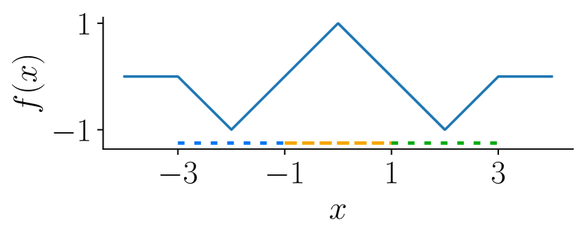
(b) Network values $f(x)$ for $x\in[-4,4]$.

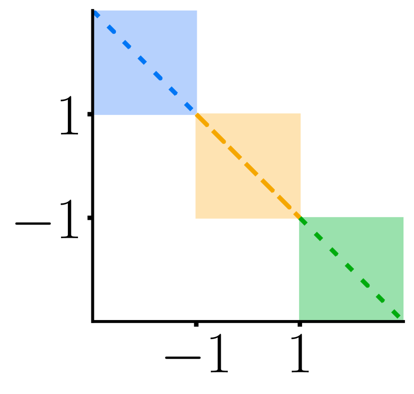
(c) 1st affine layer

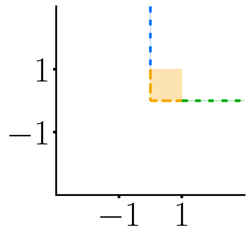
(d) 1st ReLU layer

(e) 2nd affine layer

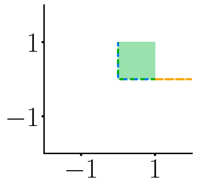
(f) 2nd ReLU layer

(g) 3rd affine layer

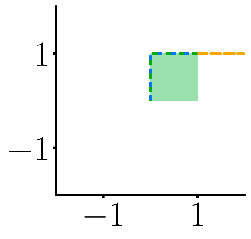
(h) 3rd ReLU layer

Figure 1. An example of a neural network which is in fact robust, yet which interval arithmetic fails to prove is robust. The three intervals $L=[-3,-1]$ ( ), $M=[-1,1]$ ( ) and $R=[1,3]$ ( ) are depicted using dashed lines in Fig. 1(b). The interval propagation through the network is shown using the rectangles, the concrete values are shown by the dashed lines. Here, after the 2nd affine layer (Fig. 1(e)) the orange and green box overlap although the orange lines do not overlap, showing the loss of precision. The output Interval is $[-1,1]$ for all three input intervals $L,M$ and $R$.

1. Introduction

As neural networks are increasingly used in safety critical environments, ensuring their behavior with formal verification has become a highly active research direction (LAL⁺, 19; HKR⁺, 20). Because neural networks are often too large for complete verification methods, incomplete analysis techniques are frequently employed (GMT⁺, 18) – these can scale to larger models though may fail to prove a property that actually holds (as demonstrated in Fig. 1). Indeed, recent progress in constructing provable neural networks has been achieved thanks to leveraging incomplete methods, and particularly interval (box) bound propagation (MGV, 18). However, while many improvements to provable defenses have been published (GDS⁺, 18; ZWC⁺, 18; ZCX⁺, 20; XTSM, 19; WSMK, 18; LSS, 21; BWL⁺, 21; SWZ⁺, 21; XZW⁺, 21) (most building on IBP), progress remains far from satisfactory: the state-of-the-art certified robust accuracy is roughly 60% on CIFAR10 (BV, 20), compared to state-of-the-art standard accuracies of above 95%. The stagnation of progress in constructing provably robust neural networks, and the importance of interval arithmetic to other areas of mathematics (Tuc, 02), has led to a fundamental question:

Do neural networks exist which can be efficiently (with interval analysis) proven correct?

(Fundamental Theoretical Question)

The first result addressing this question was investigated in BMV (20) which proved an analog to the universal approximation theorem (Cyb, 89; HSW, 89) for interval-analyzable networks. WAPJ (20) further showed that two hidden layer networks could also be interval-analyzable approximators. (Ano, 22) also demonstrated that training with interval propagation converges with high probability. While it is helpful to know that searching for networks which can be easily analyzed might not be futile, these results do not explain, and even contradict the provable training gap that is observed in practice. A preliminary negative result was shown in (WAPJ, 20): verifying the robustness of arbitrary neural networks in general and thus translating arbitrary neural networks into interval-analyzable forms is NP-hard. In our work, we provide a strong negative answer, thus explaining the provable training gap: we demonstrate that non-trivial datasets can not be classified by interval-provable networks.

Formally, given a neural network, or more generally any program, $f\colon\mathcal{X}\to\mathcal{Y}$, the goal of verification is to algorithmically prove that $f$ maps an input specification, $S_{I}\subseteq\mathcal{X}$, to a subset of an output specification, $S_{O}\subseteq\mathcal{Y}$, where $(S_{I},S_{O})$ is a member of a set $\mathcal{S}\subseteq\mathcal{P}(\mathcal{X})\times\mathcal{P}(\mathcal{Y})$, which we call the specification task. Interval analysis in particular replaces the basic operations of $f$ with interval arithmetic (Moo, 66; HJVE, 01), producing a sound interval extension, $f^{\#}\colon\text{Intervals}(\mathcal{X})\to\text{Intervals}(\mathcal{Y})$, of $f$ such that every element of $S_{I}$ is mapped by $f$ to an element of $f^{\#}(S_{I})$. As representing and computing intervals is efficient, $f$ is proven to meet the specification $(S_{I},S_{O})$ by proxy of proving $f^{\#}(\mathcal{S}_{I})\subseteq S_{O}$. The specification tasks we consider are $l_{\infty}$ robust classifications, meaning the input specifications are closed $l_{\infty}$-balls (i.e., intervals), and output specifications are either $\mathbb{R}_{>0}$ or $\mathbb{R}_{<0}$. Formally, we say an $l_{\infty}$-robustness classification $\mathcal{S}$ is complete, if for any specification $(S_{I},S_{O})\in\mathcal{S}$, there is an $l_{\infty}$-ball, the scheme, $T_{S}\supseteq S_{I}$ such that for all $l_{\infty}$-balls $B\subseteq T_{S}^{\circ}$, we have $(B,S_{O})\in\mathcal{S}$.

Main contributions. In this paper, we present the first proofs capturing key limitations (incompleteness) of interval analysis for neural networks:

• General interval impossibility (Corollary 5.12): It is impossible to construct a feed-forward $\operatorname{ReLU}$-neural network of any shape (e.g., residual, convolutional, dense, fully-connected) that is completely provably robust (Definition 5.11) with interval analysis for a simple one-dimensional dataset with only three points.

• One-layer strong interval impossibility (Theorem 4.6): Even when the requirement for complete provability is relaxed to regions that are distant from each other ($\alpha$-interval provable with $\alpha<1$ as in Definition 4.1), there are datasets with $O(\alpha^{-1})$ points that can not be provably robustly classified with one-hidden layer networks using interval analysis.

• One-layer strong interval-agnostic possibility (Proposition 5.13): completely-robust classifiers can always be constructed with one-hidden layer networks, even if they are not necessarily provably robust using interval analysis. Together with Theorem 4.6 and Corollary 5.12 this implies that the restriction that a network be analyzable with interval-arithmetic is severely limiting.

2. Problem Motivation

Studying the robustness of artificial neural networks has become an important area of research, as neural networks are increasingly deployed in safety-critical applications such as self-driving cars  (BTD⁺, 16). SZS⁺ (13) first demonstrated that neural networks classifying images can be fooled into misclassification by imperceptible pixel perturbations in an otherwise correctly classified image.

Many of these fooling techniques, known as adversarial attacks, have been developed  (CW, 17; GSS, 15; KGB, 16; SYN, 15; CH19b, ; PMG, 16; WSK, 19). To defend against these attack, methods hardening models have been proposed  (PMW⁺, 16; TKP⁺, 17; WRK, 19; SHS, 20; BIL⁺, 16; CH, 20). A particular line of research aims to provide formal guarantees (i.e., verify) that neural networks behave correctly (KBD⁺, 17; SGM⁺, 18; SGPV, 19; BWC⁺, 19; LTC, 19; WPW⁺, 18; BBS⁺, 19; ZAD, 21; LSR⁺, 21; CH19a, ; CAH, 18). As complete verification of a neural network is NP-Hard (KBD⁺, 17), the majority of modern techniques is incomplete and are based on over-approximating the behavior of a network (GMT⁺, 18). While incomplete methods can be highly efficient, it a correct classification of a network might not be provably correct, as is illustrated in Fig. 1. In fact, for naturally trained neural networks, only a small percentage of non-attackable input images are verifiable.

To improve verification rates, techniques to training networks that are amenable to verification (RSL, 18; MGV, 18; WK, 18; WSMK, 18) have been developed. While this has been a very active area of research, the state-of-the-art developed by BV (20), achieves a certified robust accuracy of 60.5% on CIFAR10 which is unsatisfactory compared to a state-of-the-art standard accuracy of above 95%.

The recent plateau of progress in closing this gap has raised concerns about whether there are theoretical limitations to neural network analysis (SYZ⁺, 19). In this work, we provide fundamental limitations, which helps to explain the significant gab between certified robust accuracy, and standard accuracy. We focus on interval analysis, as some of the most successful and widely used methods have been based on it (MGV, 18; GDS⁺, 18).

3. Background

In this section, we introduce the main concepts, and notation central to understanding our results.

3.1. General Notation

The main results in this work centers around the interval domain, which is technically the domain of axis-aligned bounding boxes, and thus we begin by describing notation related to such boxes.

Let $\mathcal{B}^{d}$, the set of closed, non-empty, axis-aligned boxes of dimension $d$ (also known as $l_{\infty}$ balls). We write the box with center $c\in\mathbb{R}^{d}$ and radius $r\in\mathbb{R}_{\geq 0}^{d}$ as $\mathbb{B}_{r}(c)\coloneqq\{x\colon\forall i\in[d]\mathpunct{.}\exists\xi\in[-1,1]\mathpunct{.}x_{i}=c_{i}+\xi r_{i}\}$. For a given box $B\in\mathcal{B}^{d}$ let $\mathcal{C}(B)$ denote its center and $\mathcal{R}(B)$ denote its radius such that $B=\mathbb{B}_{\mathcal{R}(B)}(\mathcal{C}(B))$. We also write $\mathbb{B}^{\circ}_{\epsilon}(x)\coloneqq\{y\in\mathbb{R}^{d}\colon||x-y||_{\infty}<\epsilon\}$ for $x\in\mathbb{R}^{d}$ and $\epsilon\in\mathbb{R}_{>0}$.

For a set $Y$, we write $Y|_{i}$ for the restriction of $Y$ to the dimension $i$, or more formally, $Y|_{i}\coloneqq\{y_{i}\colon y\in Y\}.$ For any bounded and non-empty set $C$, the $l_{\infty}$-hull, written $\mathcal{H}_{\infty}(C)$, is the smallest axis aligned box containing $C$. Formally, $\mathcal{H}_{\infty}(C)\coloneqq\{x\colon\forall i\in[d]\mathpunct{.}\sup(C|_{i})\leq x_{i}\leq\inf(C|_{i})\}.$

If $f\colon A\to B$ and $S\subseteq A$ we write $f[S]\coloneqq\{f(s)\colon s\in S\}$, but sometimes abuse notation and write $f(S)\coloneqq f[S]$ to avoid clutter. Similarly, we also occasionally write $f^{-1}\circ g^{-1}$ even when $f$ and $g$ are non invertible to mean $(g\circ f)^{-1}$. For any set $S$ we write $\mathcal{P}(S)$ to mean the powerset of $S$. For some positive natural $k\in\mathbb{N}$ we write $[k]\coloneqq\{1,\ldots,k\}$.

3.2. Robustness and Interval Certification (IBP)

Suppose $f\colon\mathbb{R}^{d}\to\mathbb{R}$ is some function (i.e., neural network). We say that this network assigns a label $l\in\{-1,1\}$ to a point $x\in\mathbb{R}^{d}$ if $\operatorname{sign}f(x)=l$. In our case, we discuss $l_{\infty}$-adversarial region specifications. In this case, we say that $f$ is $\epsilon$-robust around $x$ with label $l$ if $\forall x^{\prime}\in\mathbb{B}_{\epsilon}(x)\mathpunct{.}f(x^{\prime})=l$.

The goal of robustness certification is to provide a guarantee that a neural network is robust at some point. However, robustness certification does not need to inform when a neural network is not-robust at a point. This leads to efficient methods in terms of over-approximation, originally described as abstract-interpretation (CC, 77) and applied to neural networks by GMT⁺ (18).

Definition 3.1.

Given the concrete-domains $\mathcal{D}$ and $\mathcal{G}$ we say the concrete function $f\colon\mathcal{D}\to\mathcal{G}$ over-approximated by the transformed function (abstract transformer) $f^{\#}\colon\tilde{\mathcal{D}}\to\tilde{\mathcal{G}}$ with abstract-domains $\tilde{\mathcal{D}}\subseteq\mathcal{P}(\mathcal{D})$ and $\tilde{\mathcal{G}}\subseteq\mathcal{P}(\mathcal{G})$ if it is sound if for any abstract set $\mathcal{S}\in\mathcal{D}$ we have $f(\mathcal{S})\subseteq f^{\#}(\mathcal{S})$

The goal of such an over-approximation that it is possible to computationally represent and modify elements of abstract-domains, whereas it is not in general possible to do this for any subset of $\mathcal{D}$ (as it might very well be $\mathbb{R}$). We note our definitions are a slight departure from the traditional abstract interpretation literature. While typically, the abstract domain refers to the set of representations of subsets of the concrete domain, and the abstract transformer acts on these representations, we refer to the sets they represent themselves. As here we are concerned only with the question of the mathematical limitations of what is represented, and not the question of how to efficiently represent or perform computations (this is trivial for IBP), we can simplify our presentation dramatically by discussing only the represented sets and not the representations themselves.

To certify a function $f=g_{n}\circ\cdots\circ g_{1}$, where $g_{i}\colon\mathbb{R}^{d_{i}}\to\mathbb{R}^{d_{i+1}}$, is $\epsilon$-robust at $x$ using abstract interpretation, one may pick abstract-domains $\mathcal{D}_{i}\subseteq\mathcal{P}(\mathbb{R}^{d_{i}})$ and compute sound transformed functions, $g^{\#}_{1},\ldots,g^{\#}_{n}$: If $g^{\#}_{i}$ and $g^{\#}_{i+1}$ over-approximates $g_{i}$ and $g_{i+1}$ then $g^{\#}_{i}\circ g^{\#}_{i+1}$ over-approximates $g_{i+1}\circ g_{i}$. Then, given one can show for $f^{\#}=g^{\#}_{n}\circ\cdots\circ g^{\#}_{1}$, that for some $\tilde{A}\in\mathcal{D}_{1}$ such that $\mathbb{B}_{\epsilon}(x)\subseteq\tilde{A}$, it is true that $\forall\tilde{y}\in f^{\#}(\tilde{A})\mathpunct{.}\operatorname{sign}\tilde{y}=f(x)$, then one will have also shown that $\forall x^{\prime}\in\mathbb{B}_{\epsilon}(x)\mathpunct{.}\operatorname{sign}f(x^{\prime})=f(x)$.

For any function $f\colon A\to B$, we say that the perfect transformation of $f$ is $f^{\mathcal{P}}\colon\mathcal{P}(A)\to\mathcal{P}(B)$ where for any set $S\subseteq A$ we have $f^{\mathcal{P}}(S)\coloneqq f[S]$.

While the perfect transformation of $f$ is just that, always perfect, it is important to note that over-approximation is typically not precise, meaning $f(S)\subsetneq f^{\#}(S)$. In this case, it is in fact possible to not prove the guarantee, such as robustness, even if that guarantee holds for $f$.

Interval Analysis

In this paper, we focus on the Interval (or Box)-domain, and in particular, Interval Bound Propagation (IBP) (GDS⁺, 18), which is also known as interval-analysis. In this case, $\mathcal{B}^{d}$ is used as the abstract domain, $\tilde{\mathcal{D}}$, when the concrete domain is $\mathbb{R}^{d}$. An interval, $B\in\mathcal{B}^{d}$, can either be represented as a center $c\in\mathbb{R}^{d}$ and radius $r\in\mathbb{R}^{d}_{\geq 0}$ as before, or as a lower-bound and upper bound, $\iota_{l},\iota_{u}\in\mathbb{R}^{d}$ respectively such that for each dimension $j\in[d]$, we have $\iota_{l,j}\leq\iota_{u,j}$. The two representations are related as follows: $\iota_{l}=c-r$ and $\iota_{u}=c+r$, or $c=\frac{1}{2}(\iota_{l}+\iota_{u})$ and $\iota_{u}=\frac{1}{2}(\iota_{u}-\iota_{l})$.

Analyzing Neural Networks

The application of interval analysis to neural networks with $\operatorname{ReLU}$-activations is straightforward. In this paper, we consider (feed forward) neural networks defined inductively as follows:

Definition 3.2.

A $\sigma$-(neural) network with $\sigma$-activations, $f$, is any of the following forms:

• Sequential Computation: $f(x)=g_{1}(g_{2}(x))$ where $g_{1}$ and $g_{2}$ are also both $\sigma$-networks.

• Relational Duplication: $f(x)=(x,x)$.

• Non-Relational Parallel Computation: $f(x_{1},x_{2})=(g_{1}(x_{1}),g_{2}(x_{2}))$ where $g_{1}$ and $g_{2}$ are also both $\sigma$-networks.

• Constant: $f(x)=\kappa$ for some constant $\kappa\in\mathbb{R}$.

• Multiplication by a Constant: $f(x)=\kappa\cdot x$ for some constant $\kappa\in\mathbb{R}_{\neq 0}$.

• Activation: $f(x)=\sigma(x)$.

• Relational Addition: $f(x_{1},x_{2})=x_{1}+x_{2}$.

For the purposes of exploring its limits, we view IBP as method that implicitly constructs a transformed function which acts on intervals. We describe this transformed function inductively as well:

Definition 3.3 (Interval Analysis).

The interval transformation, $f^{\#}$, of a $\operatorname{ReLU}$-network $f$ is as follows:

• Sequential Abstraction: If $f(x)=g_{1}(g_{2}(x))$ then $f^{\#}(B)\coloneqq g^{\#}_{1}(g^{\#}_{2}(B))$.

• Relational Duplication: If $f(x)=(x,x)$ then $f^{\#}(B)\coloneqq B\times B$.

• Non-Relational Parallel Abstraction: If $f(x_{1},x_{2})=(g_{1}(x_{1}),g_{2}(x_{2}))$ then $f^{\#}(B)\coloneqq g^{\#}_{1}(B|_{1})\times g^{\#}_{2}(B|_{2})$.

• Constant: If $f(x)=\kappa$ for $\kappa\in\mathbb{R}$ where $m=n=1$, then $f^{\#}(B)\coloneqq\{\kappa\}$.

• Multiplication by a Constant: If $f(x)=\kappa\cdot x$ for some constant $\kappa\in\mathbb{R}_{\neq 0}$ where $m=n=1$, then $f^{\#}(B)\coloneqq\{\kappa\cdot x\}$.

• Activation: If $f(x)=\operatorname{ReLU}(x)$ (where $m=n=1$), then $f^{\#}(B)\coloneqq\{\operatorname{ReLU}(x)\colon x\in B\}$.

• Relational Addition: If $f(x_{1},x_{2})=x_{1}+x_{2}$ where $m=2$ and $n=1$, then $f^{\#}(B)\coloneqq\{a+b\colon a\in B|_{1}\wedge b\in B|_{2}\}$.

Proposition 3.4.

If $f$ is a $\operatorname{ReLU}$-network then the interval transformer, $f^{\#}$, over-approximates $f$.

4. Limits for Single Hidden Layer Networks

In this section we present an upper-bound on the number of points that can be proven to be robustly classified with interval for a single-layer network. We do this by constructing a paradoxical dataset, which we call flips. We begin by formalizing this dataset, and the notion of robust and provably robust on this dataset.

Definition 4.1.

We say:

• A flip is a point $\hat{\mathtt{x}}_{i}\coloneqq 2i$ with label $\hat{\mathtt{l}}_{i}\coloneqq(-1)^{i}$.

• $f\colon\mathbb{R}\to\mathbb{R}$ is a classifier for $k$ flips if $\forall i\in[k]\mathpunct{.}f(\hat{\mathtt{x}}_{i})=\hat{\mathtt{l}}_{i}$.

• $F\colon\mathcal{B}\to\mathcal{P}(\mathbb{R})$ is an $\alpha$-classifier for $k$ flips if $\forall i\in[k]\mathpunct{.}\forall y\in F([\hat{\mathtt{x}}_{i}-\alpha,\hat{\mathtt{x}}_{i}+\alpha])\mathpunct{.}\operatorname{sign}y=\hat{\mathtt{l}}_{i}\wedge F(\{\hat{\mathtt{x}}_{i}\})=\{\hat{\mathtt{l}}_{i}\}$.

• If $f^{\mathcal{P}}$ (the perfect transformation) is an $\alpha$-classifier for $k$ flips, we say $f$ is an $\alpha$-robust classifier for $k$ flips.

• If $f^{\#}$ (the interval transformation from Definition 3.3) is an $\alpha$-classifier for $k$ flips, then we say that $f$ is a provably $\alpha$-robust classifier for $k$ flips.

We now specify the notion of single-layer network for which we demonstrate bounds:

Definition 4.2.

A single-layer $\sigma$-network, $f\colon\mathbb{R}\to\mathbb{R}$, with $n$-neurons and $\sigma$-activations is a function with pre-activation weights, $N\in\mathbb{R}^{n}$, pre-activation bias, $b\in\mathbb{R}^{n}$, post-activation weights, $M\in\mathbb{R}^{n}$, and post-activation bias, $d\in\mathbb{R}$ (the weights and biases are known as parameters), such that $f(x)=M\cdot\sigma(Nx+b)+d$.

We note that while the Definition 3.3 defines an ordering of addition, this definition does not. While concrete-addition is associative, abstract addition is not always. However, thankfully, for the interval transformation, it is, and the bounds we demonstrate apply to any ordering of the operations.

(a) $\operatorname{ReLU}(-x)$

(b) $-\operatorname{ReLU}(-x)$

(c) $\operatorname{ReLU}(x)$

(d) $-\operatorname{ReLU}(x)$

Figure 2. The orientations of neurons captured by $L+$, $L-$, $R+$, and $R-$ for qualifying the scope of imprecision-contributions.

Definition 4.3.

Given a single-layer $\operatorname{ReLU}$-network, $f$ with $n$ neurons and pre/post-activation weights $N,M$, the imprecision-contributions of $f$ at $x$ are:

$$\mathcal{A}_{D,S}(x) \coloneqq\sum_{N_{i}x+b_{i}\geq 0\wedge M_{i}\in S\wedge N_{i}\in D}|M_{i}N_{i}|,$$

$$\text{and }\;\mathcal{I}_{D,S}(x) \coloneqq\sum_{N_{i}x+b_{i}\geq 0\wedge M_{i}\in S\wedge N_{i}\in D}M_{i}N_{i}$$

where $D$ can be the set $L\coloneqq\mathbb{R}_{\leq 0}$, the set $R\coloneqq\mathbb{R}_{\geq 0}$ or $\mathbb{R}$ and $S$ can be the set $+\coloneqq\mathbb{R}_{\geq 0}$, the set $-\coloneqq\mathbb{R}_{\leq 0}$ or $\mathbb{R}$.

Intuitively, $L+,L-,R+,R-$ correspond to the orientations that a neuron can take, as visualized in Fig. 2. $L$ (resp. $R$) results in contributions from neurons that activate as the argument $x$ of the imprecision-contribution function decreases (resp. increases). Note that $f^{\prime}(x)=\mathcal{I}_{\mathbb{R},\mathbb{R}}(x)$ if the derivative of $f$ is defined at $x$.

Lemma 4.4 (End-Neuron Imprecision-Bound).

For all $\kappa\geq 0$ and single-layer $\operatorname{ReLU}$-networks, $f$, that classify $k$-flips for $k=\lceil\kappa\rceil+5$, we have $\kappa<\max\{\mathcal{A}_{L,\mathbb{R}}(\hat{\mathtt{x}}_{1}),\mathcal{A}_{R,\mathbb{R}}(\hat{\mathtt{x}}_{k})\}$.

Proof Overview. We prove this by induction on $c\coloneqq\lfloor\kappa\rfloor$, using two simultaneous inductive invariants:

$$c \leq\mathcal{A}_{L,+}(\hat{\mathtt{x}}_{2})-\mathcal{A}_{R,+}(\hat{\mathtt{x}}_{2})+\mathcal{A}_{R,+}(\hat{\mathtt{x}}_{k})-\mathcal{A}_{L,+}(\hat{\mathtt{x}}_{k}),$$

$$\text{and }\;c \leq\mathcal{A}_{L,-}(\hat{\mathtt{x}}_{1})-\mathcal{A}_{R,-}(\hat{\mathtt{x}}_{1})+\mathcal{A}_{R,-}(\hat{\mathtt{x}}_{k-1})-\mathcal{A}_{L,-}(\hat{\mathtt{x}}_{k-1}).$$

This proof involves two key observations: (i) once imprecision-contribution in a direction has accumulated, it will only be larger for points further in that direction, (ii) one must measure not just the accumulated growth of the imprecision-contribution at the ends of the approximated data ($\hat{\mathtt{x}}_{1}$ and $\hat{\mathtt{x}}_{k}$) in the out-wards directed neurons, but the growth of the relative imprecision-contribution excluding contribution from in-wards directed neurons. We make these observations more precise in the full proof in the appendix.

(Full proof in Appendix A)

Before demonstrating our main result, we require one further lemma, used to find a specific data-point with enough accumulated imprecision contribution to cause a violation:

Lemma 4.5 (Lower-Bound on Imprecision-Contribution).

For any $a\leq 1$ and $k\geq\lceil\frac{2}{a}\rceil+5$ and single-layer $\operatorname{ReLU}$-network, $f$, that classifies $k$ flips, there is some point $j\in[k]$ such that

$$\hat{\mathtt{l}}_{j}a^{-1}(f(\hat{\mathtt{x}}_{j}+a)+f(\hat{\mathtt{x}}_{j}-a))<\mathcal{A}_{\mathbb{R},\mathbb{R}}(\hat{\mathtt{x}}_{j})+\mathcal{A}_{R,\mathbb{R}}(\hat{\mathtt{x}}_{j}-a)+\mathcal{A}_{L,\mathbb{R}}(\hat{\mathtt{x}}_{j}+a).$$

Proof Overview. By using $c\coloneqq\frac{2}{a}$ we can apply Lemma 4.4 (with $\kappa=c$), to show bounds for either the left or right-most $\hat{\mathtt{x}}$ (i.e., $j=1$ or $j=k$). For this point, we use the knowledge that the function is continuous, piecewise differentiable, to find points $l\in[\hat{\mathtt{x}}_{j}-a,\hat{\mathtt{x}}_{j}]$ and $u\in[\hat{\mathtt{x}}_{j},\hat{\mathtt{x}}_{j}+a]$ such that $\frac{f(\hat{\mathtt{x}}_{j})-f(\hat{\mathtt{x}}_{j}-a)}{a}<f^{\prime}(l)$ and $f^{\prime}(u)<\frac{f(\hat{\mathtt{x}}_{j}+a)-f(\hat{\mathtt{x}}_{j})}{a}$ so we can use that

$$f^{\prime}(l)-f^{\prime}(u)=\mathcal{I}_{\mathbb{R},\mathbb{R}}(l)-\mathcal{I}_{\mathbb{R},\mathbb{R}}(u)\leq\mathcal{A}_{L,\mathbb{R}}(\hat{\mathtt{x}}_{j}-a)-\mathcal{A}_{R,\mathbb{R}}(\hat{\mathtt{x}}_{j}+a),$$

that $-c,c<\mathcal{A}_{\mathbb{R},\mathbb{R}}(\hat{\mathtt{x}}_{j}),$ and that

$$\hat{\mathtt{l}}_{j}a^{-1}(f(\hat{\mathtt{x}}_{j}+a)+f(\hat{\mathtt{x}}_{j}-a))=\frac{f(\hat{\mathtt{x}}_{j})-f(\hat{\mathtt{x}}_{j}-a)}{a}-\frac{f(\hat{\mathtt{x}}_{j}+a)-f(\hat{\mathtt{x}}_{j})}{a}-c$$

to produce the final upper bound.

(Full proof in Appendix A)

We are now ready to show our main theorem, an upper bound on the number of flips that can be provably robustly classified with a single layer network.

Theorem 4.6 (Single-Layer Limit).

No single-layer $\operatorname{ReLU}$-network can provably $\alpha$-robustly classify $\lceil\frac{2}{\alpha}\rceil+5$ or more flips for any $\alpha\in(0,1].$

Proof Overview. The proof is by direct application of Lemma 4.5, and expansion of the definition of the derivative. We demonstrate that for the $\hat{\mathtt{x}}$ found by Lemma 4.5, the center of the box must be strictly closer to 0 than it’s radius. (Full proof in Appendix A)

5. Completely Interval Provable Classifiers are Impossible

Here we show our main result, that no neural network can be completely provably robust with interval analysis for simple functions. We first introduce the necessary lemmas and machinery that allow us show a relationship between whether the network represents an invertible function, and where there is approximation error.

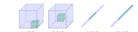
Figure 3. Visualization of the relative interior relation. The green ( ) boxes are $A$ and the purple ( ) boxes are $B$.

Counterintuitively, rather than being able to show that the transformed network in imprecise for a specific input box (i.e., that for a specific box $B$, we know $f[B]\subsetneq f^{\#}(B)$), we must, for any input box $B$ containing non-invertible points on its surface, find an input box, $A$, that is a strict subsets of $B$ (by a particular notion of strict defined below), such that $f(B)\subseteq f^{\#}(A)$. The fact that $A$ is a very strict subset of $B$ implies that interval analysis is imprecise enough on the network such that it can not be used to prove desired properties of $B$ (such that $f$ is completely robust for $B$). It is however crucial that $A$ not be required to be too strict a subset of $B$. One might be tempted to find subsets of the topological interior of $B$. This however leads to significant technical issues: we need to have a notion of strict subset that applies even when some of the neurons in the network are unused (and zero). One can imagine the set representing the possible activations of those neurons as a lower dimensional surface embedded in a higher dimensional space, as in the case of Fig. 3(c) and (d). In this case, the interior of $B$ would be empty, even though we might have identified a subset of it that induces imprecision.

5.1. The Relative Subset Relation

We begin by formalizing the intuitive concept from Fig. 3 using the notion of relative interior, and demonstrating some useful lemmas related to it. First, recall for a set $S\subseteq\mathbb{R}^{d}$ that the affine hull of $S$, written $\operatorname{aff}(S)$ is the smallest linear-subspace of $\mathbb{R}^{d}$ that contains $S$.

Definition 5.1.

We define relative interior as $\operatorname{relint}(S)\coloneqq\{x\in S\colon\exists\epsilon>0\mathpunct{.}\mathbb{B}^{\circ}_{\epsilon}(x)\cap\operatorname{aff}(S)\subseteq S\}$

We note that if $S\in\mathcal{B}^{d}$, the set of closed, non-empty, axis-aligned boxes of dimension $d$, we can restate the relative interior as $\operatorname{relint}(S)=\{x\in S\colon\forall i\in[d]\mathpunct{.}x\in S|_{i}^{\circ}\cup\{\mathcal{C}(S)_{i}\}\},$ where $S|_{i}^{\circ}$ is the interior of $S$’s restriction to dimension $i$.

Definition 5.2 (Relative Subset).

$A$ is a relative subset of $B$, written $A\sqsubset B$, if and only if $A\subseteq\operatorname{relint}(B)$.

We note again, that if $A,B\in\mathcal{B}^{d}$, we can rephrase $A\sqsubset B$ as follows: $A\subseteq B$ and for each dimension, $i$, where $B|_{i}^{\circ}$ isn’t empty, $A|_{i}\subseteq B|_{i}^{\circ}$ or more concisely, $\forall i\in[d]\mathpunct{.}(B|_{i}^{\circ}\neq\emptyset\implies A|_{i}\subseteq B|_{i}^{\circ}).$ In particular, in one dimension, for real intervals $[a,b]$ and $[b,c]$ we have $[a,b]\sqsubset[a^{\prime},b^{\prime}]$ if and only if $a<a^{\prime}\leq b^{\prime}<b$ or $a=a^{\prime}=b^{\prime}=b$.

Let $A,A^{\prime},B,B^{\prime},C$ be bounded and non-empty subsets of $\mathbb{R}^{d}$ in the following lemmas (the proofs of which can be found in Section B.1):

Lemma 5.3 (Respects Projection).

$A\sqsubset B$ implies $A|_{i}\sqsubset B|_{i}$.

Lemma 5.4 (Respects Cartesian Product).

$A\sqsubset B$ and $A^{\prime}\sqsubset B^{\prime}$ implies $A\times A^{\prime}\sqsubset B\times B^{\prime}$.

Lemma 5.5 (Downward Union).

$A\sqsubset C$ and $B\sqsubset C$ implies $A\cup B\sqsubset C$.

Lemma 5.6 (Downward Hull).

$C\in\mathcal{B}^{d}$ and $A\sqsubset C$ implies $\mathcal{H}_{\infty}(A)\sqsubset C$.

The following two trivial lemmas are trivial, and we frequently use them without mention:

Lemma 5.7 (Singleton Reflexivity).

$\{a\}\sqsubset\{a\}$.

Lemma 5.8 (Center-Singleton is Always a Relative Subset).

$A\in\mathcal{B}^{d}$ implies $\{\mathcal{C}(A)\}\sqsubset A$.

It is important to note that some simple related properties counterintuitively do not always hold. Namely, if $A\sqsubset B$ and $B\subseteq C$ it is not always the case that $A\sqsubset C$. Furthermore, if $A\sqsubset B$ and $A^{\prime}\sqsubset B^{\prime}$ it is not always the case that $\mathcal{H}_{\infty}(A\cup A^{\prime})\sqsubset\mathcal{H}_{\infty}(B\cup B^{\prime})$.

5.2. Inversion With Respect to The Relative Subset Relation

Here we demonstrate that neural networks can loosely invert sets with respect to the relative subset relation. More formally, for any neural network $f$ with $\operatorname{ReLU}$-activations, one can essentially always find a strict subset, $X^{\prime}$ of the relative interior of a box $X$ that the neural network maps to a superset of a specified subset $Y$ of the relative interior of the $l_{\infty}$-hull of $f(X)$.

Lemma 5.9 (Concrete Relative Inversion).

Suppose $f$ is a feed-forward network with $\operatorname{ReLU}$-activations and $Y,X^{\prime}\in\mathcal{B}^{d}$ and $X$ is compact and non-empty. Then

$Y\sqsubset\mathcal{H}_{\infty}(f(X))\implies\exists X^{\prime}\sqsubset\mathcal{H}_{\infty}(X)\mathpunct{.}Y\subseteq f^{\#}(X^{\prime}).$

Proof Overview. (Full Proof in Section B.2) The proof is by structural induction on the construction of $f$. We use the lemma itself as the induction hypothesis. Below we outline three key cases of the structural induction: sequential computations, relational parallel computations, and $\operatorname{ReLU}$:

Case: $f=g\circ h$. (Sequential Computation) Subproof. By definition, $Y\sqsubset\mathcal{H}_{\infty}(g\circ h(X))$. Thus, there is some $H\sqsubset\mathcal{H}_{\infty}(h(X))$ such that $Y\subseteq g^{\#}(H)$ by the induction hypothesis on $g$. Applying the induction hypothesis again with the network $h$, we get a set $X^{\prime}\sqsubset\mathcal{H}_{\infty}(X)$ such that $H\subseteq h^{\#}(X^{\prime})$. Thus, $Y\subseteq g^{\#}(H)\subseteq g^{\#}\circ h^{\#}(X^{\prime})=f^{\#}(X^{\prime})$. ∎

Case: $f(x)=(x,x)$. (Relational Duplication) Subproof. In this case, we know $Y|_{1}\sqsubset\mathcal{H}_{\infty}(X)$ and $Y|_{2}\sqsubset\mathcal{H}_{\infty}(X)$ by Lemma 5.3. By Lemma 5.5, we know $X^{\prime}\coloneqq\mathcal{H}_{\infty}(Y|_{1}\cup Y|_{2})$ is a relative subset of $\mathcal{H}_{\infty}(X)$, and also that $Y\subseteq X^{\prime}\times X^{\prime}=f^{\#}(X^{\prime})$. ∎

Case: $f(x_{1},x_{2})=(g_{1}(x_{1}),g_{2}(x_{2}))$. (Non-Relational Parallel Computation) Subproof. We know $Y|_{1}\sqsubset\mathcal{H}_{\infty}(g_{1}(X|_{1}))$ and $Y|_{2}\sqsubset\mathcal{H}_{\infty}(g_{1}(X|_{1}))$, so we can apply the induction hypothesis twice to produce $L\sqsubset\mathcal{H}_{\infty}(X|_{1})$ and $R\sqsubset\mathcal{H}_{\infty}(X|_{2})$ such that $Y|_{1}\subseteq g^{\#}_{1}(L)$ and $Y|_{2}\subseteq g^{\#}_{1}(R)$. We choose $X^{\prime}=L\times R$. By Lemma 5.4, we have $X^{\prime}\sqsubset\mathcal{H}_{\infty}(X)$. Then $Y\subseteq g^{\#}_{1}(X^{\prime}|_{1})\times g^{\#}_{2}(X^{\prime}|_{2})=f^{\#}(X^{\prime})$. ∎

Case: $f(x)=\operatorname{ReLU}(x)$. (Activation) Subproof. We know here that $f\colon\mathbb{R}\to\mathbb{R}$ which simplifies the proof. In this case, $l_{\infty}$-hull of $f(X)$ must either be a subset of $\mathbb{R}_{\geq 0}$ so either $Y$ is the singleton set containing zero, or a subset of $\mathbb{R}_{>0}$. In the first case, we pick $X^{\prime}$ to be an easy-to-pick (the singleton set containing center as in Lemma 5.8) relative subset of the hull of $X$. Otherwise, we can pick $Y$ itself, since $\operatorname{ReLU}(Y)=Y\subseteq\mathcal{H}_{\infty}(X)$. ∎ (Further Cases in Section B.2)

5.3. Impossibility for Non-Invertibility

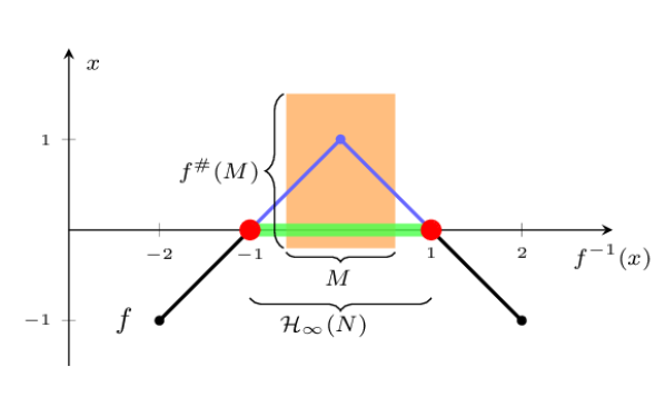
Figure 4. A visualization of the claims of Theorem 5.10. The neural network, $f$ is classifying three flips $\hat{\mathtt{x}}_{-1},\hat{\mathtt{x}}_{0}$ and $\hat{\mathtt{x}}_{1}$ (i.e., $D=\{(-2,-1),(0,1),(2,-1)\}$ as in Corollary 5.12). Here, $x=0$ is the non-invertability and $f^{-1}(x)=\{-1,1\}$. These two points mapping to $x$, which constitute $N\subseteq f^{-1}(x)$, are marked in red ( ). The $l_{\infty}$-hull, $\mathcal{H}_{\infty}(N)$, is marked in green ( ). The perfect approximation of $f$ on $\mathcal{H}_{\infty}(N)$ (i.e., $\{(v,f(v))\colon v\in N\}$) is marked in blue ( ). We can see that the interval approximation of the relative interior box $M\sqsubset\mathcal{H}_{\infty}(N)$ looses precision by looking at the orange region ( ).

We now prove our central result, that non-invertible neural networks necessarily induce approximation imprecision. Essentially, as visualized in Fig. 4, we show that there is a box, $M$ which is a relative subset (i.e., usually very strict subset) of the $l_{\infty}$-hull of any region for which the network is entirely not injective, such that analyzing the network with $M$ includes any of the non-invertible points in the inferred approximation.

The key idea is that while there might be non-invertible points on the boundary of a region, $M$ does not include those points, since it is a relative subset. Thus, we can use this theorem to infer areas where analyzing the network produces approximations that include points that aren’t in the concrete, or true, set of possible network outputs.

Theorem 5.10 (Non-Invertibility Induces Interval Imprecision).

Suppose $f\colon\mathbb{R}^{n}\to\mathbb{R}^{m}$ is a feed-forward network with $\operatorname{ReLU}$-activations and $x\in\mathbb{R}^{m}$ and $N\subseteq f^{-1}(x)$ is compact and non-empty. Then (assuming $M$ is a box):

$\exists M\sqsubset\mathcal{H}_{\infty}(N)\mathpunct{.}x\in f^{\#}(M).$

Proof Overview. (Full Proof in Section B.2) Again, the proof is by structural induction on the construction of $f$, using the lemma itself as the induction hypothesis. Below we outline three key cases: sequential computations, relational parallel computations, and addition:

Case: $f=g\circ h$ (Sequential Computation) Subproof. We know that $N\subseteq h^{-1}\circ g^{-1}(x)$, and thus can use the induction hypothesis on $h$ to produce $M^{\prime}\sqsubset\mathcal{H}_{\infty}(h(N))$ such that $x\in g^{\#}(M^{\prime})$. By Lemma 5.9, we know that there is some $M\sqsubset\mathcal{H}_{\infty}(N)$ such that $M^{\prime}\subseteq h^{\#}(M)$ and thus that $x\in g^{\#}\circ h^{\#}(M)$. ∎

Case: $f(y)=(y,y)$. (Relational Duplication) Subproof. We have $N\subseteq\{x_{1}\}\cap\{x_{2}\}$ so $N=\{x_{1}\}$. By singleton reflexivity, $N\sqsubset\mathcal{H}_{\infty}(N)$. Thus, $x\in f^{\#}(N)$. ∎

Case: $f(x_{1},x_{2})=(g_{1}(x_{1}),g_{2}(x_{2}))$. (Non-Relational Parallel Computation) Subproof. First we know $N|_{1}\subseteq g_{1}^{-1}(x_{1})$ and $N|_{2}\subseteq g_{2}^{-1}(x_{2})$ by projection and that $N|_{1}$ and $N|_{2}$ are still compact and non-empty. Thus, by the induction hypothesis twice we see that there are boxes $M_{1}\sqsubset\mathcal{H}_{\infty}(N|_{1})$ and $M_{2}\sqsubset\mathcal{H}_{\infty}(N|_{2})$ such that $x_{1}\in g_{1}^{\#}(M_{1})$ and $x_{2}\in g_{2}^{\#}(M_{2})$. Then $M_{1}\times M_{2}\sqsubset\mathcal{H}_{\infty}(N)$ by Lemma 5.4. Then $x_{1}\in g_{1}^{\#}(M_{1}\times M_{2})$ and $x_{2}\in g_{2}^{\#}(M_{1}\times M_{2})$ by soundness. Thus, there is some box $M\sqsubset\mathcal{H}_{\infty}(N)$ such that $x\in f^{\#}(M)$. ∎

Case: $f(y_{1},y_{2})=y_{1}+y_{2}$. (Addition) Subproof. Because $f\colon\mathbb{R}^{2}\to\mathbb{R}$, we know $f^{-1}(x)=\{(a,x-a)\colon a\in\mathbb{R}\}$. We can pick $M=\{\mathcal{C}(\mathcal{H}_{\infty}(N))\}$ and demonstrate that $M\sqsubset\mathcal{H}_{\infty}(N)$ and that $x\in f^{\#}(M)$. ∎

(Further Cases in Section B.2)

5.4. Implications and Corollaries

Here we demonstrate implications of this result, such as that no neural network can completely (as defined below), and provably robustly with interval, classify every dataset.

Definition 5.11.

We say that a neural network $f\colon\mathbb{R}^{d}\to\mathbb{R}$ is a completely $\nu$-(provable) robust classifier for points $x_{1},\ldots,x_{n}\in\mathbb{R}^{d}$ and labels $l_{1},\ldots,l_{n}\in\{-1,1\}$ if given $\delta=\frac{1}{2}\min_{i\neq j}||x_{i}-x_{j}||_{\infty}$ then $\forall\epsilon<\nu\delta\mathpunct{.}\forall i\in[d]\mathpunct{.}f(\mathbb{B}_{\epsilon}(x_{i}))l_{i}>0.$ If it is provable then we also have that $\forall i\in[d]\mathpunct{.}f^{\#}(\mathbb{B}_{\epsilon}(x_{i}))l_{i}>0.$

We note that the specification task implicitly induced by this definition is complete as defined by the more general notion in the introduction.

Corollary 5.12 (Completely Provable Classifiers are Impossible).

There is no feed forward $\operatorname{ReLU}$-network that is a completely $1$-provable classifier for the dataset $D=\{(-2,-1),(0,1),(2,-1)\}$.

Proof. Suppose $f\colon\mathbb{R}\to\mathbb{R}$ is a completely $1$-provable interpolator for this dataset. Then by continuity we know that $f(-1)=f(1)=0$, and thus that $\{-1,1\}\subseteq f^{-1}(0)$ (which is a compact non-empty set). Then by application of Theorem 5.10, there is some set $M\sqsubset\mathcal{H}_{\infty}(\{-1,1\})$ such that $0\in f^{\#}(M)$. Rephrased, this means that there are $a,b\in(-1,1)$ such that $0\in f^{\#}([a,b])$. This contradicts with the definition of a completely $1$-provable classifier however. ∎

Proposition 5.13 (Single-Layer Completely Robust Classifiers Always Exist).

For any dataset of $n$ points $x_{i}\in\mathbb{R}$ and labels $l_{i}\in\{-1,1\}$ there is a one-hidden-layer $\operatorname{ReLU}$-network that completely robustly (but not necessarily provably) classifies it.

Proof. We present the construction explicitly. Let $\delta\coloneqq\min\{|x_{i}-x_{j}|\colon i\neq j\}$ in

$$f(y)\coloneqq\sum_{i=1}^{n}l_{i}\left(\operatorname{ReLU}\left[\frac{1}{\delta}(y-(x_{i}-\delta))\right]-\operatorname{ReLU}\left[\frac{2}{\delta}(y-x_{i})\right]+\operatorname{ReLU}\left[\frac{1}{\delta}(y-(x_{i}+\delta))\right]\right)$$

One can check that this works by plugging in $x_{j}$, although a full proof is by induction. While this is not immediately of the form described for one-hidden layer networks, one can see easily how to algebraically convert this into that form. Because we only care about the robustness, and not interval provability of $f$, this is sufficient. ∎

6. Discussion and Future Work

While we limited the scope of our discussion to $\operatorname{ReLU}$-activations, we note that our theorems extetend trivially to any monotone bounded activation. However, we observe that non-monotonic activations functions (such as absolute value) do not admit the same forms of theorems. Our preliminary experiments however indicate that substituting $\operatorname{ReLU}$ with these activation functions does not result in easier training or provability. This suggests that there are more general version of the the theorems presented here, in particular relating the difficulty of program synthesis with the relational expressiveness of the domain used to verify the specification.

7. Conclusion

In this paper, we proved two theorems that show limits in the expressiveness of interval provable neural networks. We showed that no $\operatorname{ReLU}$-network can completely provably classify simple one-dimensional datasets containing only three points. This indicates a fundamental loss of precision whenever $\operatorname{ReLU}$-networks are analyzed using interval arithmetic, which can not be regained, no matter the network. Further, we showed that a single hidden layer $\operatorname{ReLU}$-network can not provably classify simple datasets even without the requirement for completeness, which is in stark contrast to classical universal approximation theorems, where a single hidden layer is sufficient. This shows that the approximative capabilities of interval provable networks are lower compared to standard neural networks.

Appendix A Extended Proofs for Single Hidden Layer Network Results

Here we restate the theorems and show the full proofs for the results in Section 4. See 4.4 Proof of 4.4. We prove this by induction on $c$.

Induction Hypothesis: Given $c\in\mathbb{N}\cup\{0,-1,-2\}$ there is some even natural number $k\leq\operatorname{ReLU}(c+2)+2$ such that for any single-layer $\operatorname{ReLU}$-network, $f$ that classifies $k$ flips we have

$$c \leq\mathcal{A}_{L,+}(\hat{\mathtt{x}}_{2})-\mathcal{A}_{R,+}(\hat{\mathtt{x}}_{2})+\mathcal{A}_{R,+}(\hat{\mathtt{x}}_{k})-\mathcal{A}_{L,+}(\hat{\mathtt{x}}_{k}),$$

$$\text{and }\;c \leq\mathcal{A}_{L,-}(\hat{\mathtt{x}}_{1})-\mathcal{A}_{R,-}(\hat{\mathtt{x}}_{1})+\mathcal{A}_{R,-}(\hat{\mathtt{x}}_{k-1})-\mathcal{A}_{L,-}(\hat{\mathtt{x}}_{k-1}).$$

Base Case: Suppose $c\leq 0$. Subproof. Pick $k=2$. Then

$$\mathcal{A}_{L,+}(\hat{\mathtt{x}}_{2})-\mathcal{A}_{R,+}(\hat{\mathtt{x}}_{2})+\mathcal{A}_{R,+}(\hat{\mathtt{x}}_{2})-\mathcal{A}_{L,+}(\hat{\mathtt{x}}_{2}) =0\geq c,\;\text{ and }$$

$$\mathcal{A}_{L,-}(\hat{\mathtt{x}}_{1})-\mathcal{A}_{R,-}(\hat{\mathtt{x}}_{1})+\mathcal{A}_{R,-}(\hat{\mathtt{x}}_{2-1})-\mathcal{A}_{L,-}(\hat{\mathtt{x}}_{2-1}) =0\geq c.$$

∎

Induction Step: Suppose $c>0$, and the induction hypothesis holds for $c-2$. Subproof. Then there is some even natural $k^{\prime}\leq\operatorname{ReLU}(c-2+2)+2$ such that for any single-layer $\operatorname{ReLU}$-network, $f$, that is a classifier for $k^{\prime}$ flips we have

$$c-2 \leq\mathcal{A}_{L,+}(\hat{\mathtt{x}}_{2})-\mathcal{A}_{R,+}(\hat{\mathtt{x}}_{2})+\mathcal{A}_{R,+}(\hat{\mathtt{x}}_{k^{\prime}})-\mathcal{A}_{L,+}(\hat{\mathtt{x}}_{k^{\prime}}),$$

$$\text{and }\;c-2 \leq\mathcal{A}_{L,-}(\hat{\mathtt{x}}_{1})-\mathcal{A}_{R,-}(\hat{\mathtt{x}}_{1})+\mathcal{A}_{R,-}(\hat{\mathtt{x}}_{k^{\prime}-1})-\mathcal{A}_{L,-}(\hat{\mathtt{x}}_{k^{\prime}-1}).$$

Pick $k=k^{\prime}+2$. Then $k$ is even, and $k\leq\operatorname{ReLU}(c)+4\leq\operatorname{ReLU}(c+2)+2$ since $c>0$.

Let $f$ be any single-layer $\operatorname{ReLU}$-network that classifies $k$ flips. Then $f$ also classifies $k^{\prime}$ flips.

We only show the positive bound, that $c\leq\mathcal{A}_{L,+}(\hat{\mathtt{x}}_{2})-\mathcal{A}_{R,+}(\hat{\mathtt{x}}_{2})+\mathcal{A}_{R,+}(\hat{\mathtt{x}}_{k})-\mathcal{A}_{L,+}(\hat{\mathtt{x}}_{k})$.

The proof for the negative bound is analogous.

There must be some point $l\in[\hat{\mathtt{x}}_{k^{\prime}},\hat{\mathtt{x}}_{k^{\prime}+1}]$ such that $f^{\prime}(l)\leq-1$ by the mean value theorem (since $\operatorname{ReLU}$-networks are continuous) and because $f(\hat{\mathtt{x}}_{k^{\prime}})=1=-f(\hat{\mathtt{x}}_{k^{\prime}+1})$.

Similarly, there must be some point $u\in[\hat{\mathtt{x}}_{k^{\prime}+1},\hat{\mathtt{x}}_{k}]$ such that $1\leq f^{\prime}(u)$. Thus,

$$2 \leq f^{\prime}(u)-f^{\prime}(l)$$

$$\leq\mathcal{I}_{L,+}(u)+\mathcal{I}_{L,-}(u)+\mathcal{I}_{R,+}(u)+\mathcal{I}_{R,-}(u)$$

$$-\mathcal{I}_{L,+}(l)-\mathcal{I}_{L,-}(l)-\mathcal{I}_{R,+}(l)-\mathcal{I}_{R,-}(l).$$

We know $\mathcal{I}_{L,-}(u)-\mathcal{I}_{L,-}(l)\leq 0$ and $\mathcal{I}_{R,-}(u)-\mathcal{I}_{R,-}(l)\leq 0$ and $\mathcal{I}_{L,+}(t)=-\mathcal{A}_{L,+}(t)$ and $\mathcal{I}_{R,+}(t)=\mathcal{A}_{R,+}(t)$ for any $t$ so

$$2 \leq-\mathcal{A}_{L,+}(u)+\mathcal{A}_{R,+}(u)$$

$$+\mathcal{A}_{L,+}(l)-\mathcal{A}_{R,+}(l).$$

We also know $\mathcal{A}_{L,S}(t)$ increases as $t$ decreases and $\mathcal{A}_{R,S}(t)$ increases as $t$ increases, so

$$2 \leq-\mathcal{A}_{L,+}(\hat{\mathtt{x}}_{k})+\mathcal{A}_{R,+}(\hat{\mathtt{x}}_{k})$$

$$+\mathcal{A}_{L,+}(\hat{\mathtt{x}}_{k^{\prime}})-\mathcal{A}_{R,+}(\hat{\mathtt{x}}_{k^{\prime}}).$$

By combining with the positive inductive bound, we get

$$(c-2)+2=c \leq\mathcal{A}_{L,+}(\hat{\mathtt{x}}_{2})-\mathcal{A}_{R,+}(\hat{\mathtt{x}}_{2})+\mathcal{A}_{R,+}(\hat{\mathtt{x}}_{k^{\prime}})-\mathcal{A}_{L,+}(\hat{\mathtt{x}}_{k^{\prime}})$$

$$-\mathcal{A}_{L,+}(\hat{\mathtt{x}}_{k})+\mathcal{A}_{R,+}(\hat{\mathtt{x}}_{k})+\mathcal{A}_{L,+}(\hat{\mathtt{x}}_{k^{\prime}})-\mathcal{A}_{R,+}(\hat{\mathtt{x}}_{k^{\prime}})$$

$$\leq\mathcal{A}_{L,+}(\hat{\mathtt{x}}_{2})-\mathcal{A}_{R,+}(\hat{\mathtt{x}}_{2})-\mathcal{A}_{L,+}(\hat{\mathtt{x}}_{k})+\mathcal{A}_{R,+}(\hat{\mathtt{x}}_{k}),$$

which proves the positive bound of the induction hypothesis for $c$. ∎

Thus, by induction, we find that there is some $k\leq\lceil c\rceil+5$ such that, after removing the negative terms and increasing by swapping $\hat{\mathtt{x}}_{2}$ with $\hat{\mathtt{x}}_{1}$ and $\hat{\mathtt{x}}_{k-1}$ with $\hat{\mathtt{x}}_{k}$:

$$c+1 \leq\mathcal{A}_{L,+}(\hat{\mathtt{x}}_{1})+\mathcal{A}_{R,+}(\hat{\mathtt{x}}_{k}),$$

$$\text{and }\;c+1 \leq\mathcal{A}_{L,-}(\hat{\mathtt{x}}_{1})+\mathcal{A}_{R,-}(\hat{\mathtt{x}}_{k}).$$

Summing these equations together gives us:

$$2c+2\leq\mathcal{A}_{L,+}(\hat{\mathtt{x}}_{1})+\mathcal{A}_{R,+}(\hat{\mathtt{x}}_{k})+\mathcal{A}_{L,-}(\hat{\mathtt{x}}_{1})+\mathcal{A}_{R,-}(\hat{\mathtt{x}}_{k})=2\max\{\mathcal{A}_{L,\mathbb{R}}(\hat{\mathtt{x}}_{1}),\mathcal{A}_{R,\mathbb{R}}(\hat{\mathtt{x}}_{k})\},$$

and thus that $c<\max\{\mathcal{A}_{L,\mathbb{R}}(\hat{\mathtt{x}}_{1}),\mathcal{A}_{R,\mathbb{R}}(\hat{\mathtt{x}}_{k}).$ ∎

See 4.5 Proof of 4.5. Let $k\geq\lceil 2a^{-1}\rceil+5,$ and define $c\coloneqq\frac{2}{a}.$ Because $k\geq\lceil|c|\rceil+5$, we can use Lemma 4.4 to get that $|c|<\max\{\mathcal{A}_{L,\mathbb{R}}(\hat{\mathtt{x}}_{1}),\mathcal{A}_{R,\mathbb{R}}(\hat{\mathtt{x}}_{k})\}$.

For convenience, we define $\tilde{f}_{L}(x)=a^{-1}(f(x)-f(x-a))$ and $\tilde{f}_{R}(x)=a^{-1}(f(x+a)-f(x))$.

We only show the proof when $|c|<\mathcal{A}_{L,\mathbb{R}}(\hat{\mathtt{x}}_{1})$, the other case is analogous, but picking $j=k$.

In this case we know $0<\mathcal{A}_{L,\mathbb{R}}(\hat{\mathtt{x}}_{1})$ and thus,

$$\hat{\mathtt{l}}_{1}a^{-1}(f(\hat{\mathtt{x}}_{1}+a)+f(\hat{\mathtt{x}}_{1}-a))\leq\tilde{f}_{L}(\hat{\mathtt{x}}_{1})-\tilde{f}_{R}(\hat{\mathtt{x}}_{1})-c.$$

There must be a point $l\in[\hat{\mathtt{x}}_{1}-a,\hat{\mathtt{x}}_{1}]$ such that $\tilde{f}_{L}(l)\leq f^{\prime}(l)$ and a point $u\in[\hat{\mathtt{x}}_{1},\hat{\mathtt{x}}_{1}+a]$ such that $f^{\prime}(u)\leq\tilde{f}_{R}(u).$

We can thus derive, in a manner similar to what is seen in Lemma 4.4:

$$\tilde{f}_{L}(\hat{\mathtt{x}}_{1})-\tilde{f}_{R}(\hat{\mathtt{x}}_{1})\leq f^{\prime}(l)-f^{\prime}(u) \leq\mathcal{I}_{L,+}(l)+\mathcal{I}_{L,-}(l)+\mathcal{I}_{R,+}(l)+\mathcal{I}_{R,-}(l)$$

$$-\mathcal{I}_{L,+}(u)-\mathcal{I}_{L,-}(u)-\mathcal{I}_{R,+}(u)-\mathcal{I}_{R,-}(u)$$

$$\leq\mathcal{I}_{L,-}(l)-\mathcal{I}_{R,-}(u)$$

$$\leq\mathcal{A}_{L,\mathbb{R}}(\hat{\mathtt{x}}_{1}-a)-\mathcal{A}_{R,\mathbb{R}}(\hat{\mathtt{x}}_{1}+a).$$

$\tilde{f}_{L}(\hat{\mathtt{x}}_{1})-\tilde{f}_{L}(\hat{\mathtt{x}}_{1})-c<\mathcal{A}_{\mathbb{R},\mathbb{R}}(\hat{\mathtt{x}}_{1})+\mathcal{A}_{L,\mathbb{R}}(\hat{\mathtt{x}}_{1}-a)+\mathcal{A}_{R,\mathbb{R}}(\hat{\mathtt{x}}_{1}+a)$ as $-c\leq|c|<\mathcal{A}_{L,\mathbb{R}}(\hat{\mathtt{x}}_{1})\leq\mathcal{A}_{\mathbb{R},\mathbb{R}}(\hat{\mathtt{x}}_{1})$. ∎

See 4.6 Proof of 4.6. Suppose $\alpha\in(0,1]$, and assume, for the sake of contradiction, that $f$ is a single-layer $\operatorname{ReLU}$-network with weights $N,M$ and biases $b,d$ that provably $\alpha$-robustly classifies $\lceil\frac{2}{\alpha}\rceil+5$ flips.

We begin the proof by labeling the intermediate states of interval analysis for a point $\hat{\mathtt{x}}_{j}$ with interval radius $\alpha$ of the network $f$:

$$v^{-}_{\alpha,j} \coloneqq\operatorname{ReLU}(N\hat{\mathtt{x}}_{j}+b-|N|\alpha)$$

$$v^{+}_{\alpha,j} \coloneqq\operatorname{ReLU}(N\hat{\mathtt{x}}_{j}+b+|N|\alpha)$$

$$w_{\alpha,j} \coloneqq v^{+}_{j,\alpha}-v^{-}_{j,\alpha}$$

$$c_{\alpha,j} \coloneqq v^{+}_{j,\alpha}+v^{-}_{j,\alpha}$$

$$f^{\#}(\langle\hat{\mathtt{x}}_{j},\alpha\rangle) \coloneqq\langle\frac{1}{2}Mc_{\alpha,j}+d,\frac{1}{2}|M|w_{\alpha,j}\rangle,$$

where the notation $|X|$ means the point-wise absolute value (i.e., $|X|_{i}=|X_{i}|$).

Then our assumption for contradiction tells us that for any $j\in[k]$ we know that $(-1)^{j}(Mc_{\alpha,j}+2d)\geq|M|w_{\alpha,j}.$

Let $j$ be such that Lemma 4.5 tells us has $\hat{\mathtt{l}}_{j}\alpha^{-1}(f(\hat{\mathtt{x}}_{j}+\alpha)+f(\hat{\mathtt{x}}_{j}-\alpha))<\mathcal{A}_{\mathbb{R},\mathbb{R}}(\hat{\mathtt{x}}_{j})+\mathcal{A}_{R,\mathbb{R}}(\hat{\mathtt{x}}_{j}-\alpha)+\mathcal{A}_{L,\mathbb{R}}(\hat{\mathtt{x}}_{j}+\alpha)$.

We note that by expanding the definitions, sums, and meaning of absolute value, we can derive that $Mc_{\alpha,j}+2d=M(v^{+}_{\alpha,j}+v^{+}_{\alpha,j})+2d=f(\hat{\mathtt{x}}_{j}+\alpha)+f(\hat{\mathtt{x}}_{j}-\alpha)$. so our assumption for contradiction thus implies $|M|w_{\alpha,j}\leq(-1)^{j}(Mc_{\alpha,j}+2d)=(-1)^{j}(f(\hat{\mathtt{x}}_{j}+\alpha)+f(\hat{\mathtt{x}}_{j}-\alpha)$.

We perform the following deduction:

$$(-1)^{j}(f(\hat{\mathtt{x}}_{j}+\alpha)+f(\hat{\mathtt{x}}_{j}-\alpha)) \geq\sum_{N_{i}\hat{\mathtt{x}}_{j}+b_{i}\geq-\alpha|N_{i}|}|M_{i}|(N_{i}x+b_{i}+\alpha|N_{i}|)-|M|v^{-}_{\alpha,j}$$

$$\geq\sum_{N_{i}\hat{\mathtt{x}}_{j}+b_{i}\geq 0}|M_{i}|(N_{i}x+b_{i}+\alpha|N_{i}|)-|M|v^{-}_{\alpha,j}$$

$$\geq|M|\operatorname{ReLU}(Nx+b)+\sum_{N_{i}\hat{\mathtt{x}}_{j}+b_{i}\geq 0}\alpha|M_{i}N_{i}|$$

$$-\sum_{N_{i}\hat{\mathtt{x}}_{j}+b_{i}\geq\alpha|N_{i}|}|M_{i}|(N_{i}x+b_{i}-\alpha|N_{i}|)$$

$$\geq\sum_{N_{i}\hat{\mathtt{x}}_{j}+b_{i}\geq 0}\alpha|M_{i}N_{i}|+\sum_{N_{i}\hat{\mathtt{x}}_{j}+b_{i}\geq\alpha|N_{i}|}\alpha|M_{i}N_{i}|$$

$$\geq\alpha\left(\sum_{N_{i}\hat{\mathtt{x}}_{j}+b_{i}\geq 0}|M_{i}N_{i}|+\sum_{N_{i}\hat{\mathtt{x}}_{j}+b_{i}\geq\alpha|N_{i}|}|M_{i}N_{i}|\right)$$

$$\geq\alpha(\mathcal{A}_{\mathbb{R},\mathbb{R}}(\hat{\mathtt{x}}_{j})+\mathcal{A}_{R,\mathbb{R}}(\hat{\mathtt{x}}_{j}-\alpha)+\mathcal{A}_{L,\mathbb{R}}(\hat{\mathtt{x}}_{j}+\alpha))$$

$$\geq\hat{\mathtt{l}}_{j}(f(\hat{\mathtt{x}}_{j}+\alpha)+f(\hat{\mathtt{x}}_{j}-\alpha))$$

which is a contradiction. ∎

Appendix B Extended Proofs for General Impossibility Results

Here we restate the theorems and show the full proofs for the results in Section 5.

B.1. Proofs for Relative Interior Lemmas

In the following lemmas, let $A,A^{\prime},B,B^{\prime},C$ be bounded and non-empty subsets of $\mathbb{R}^{d}$:

See 5.3 Proof of 5.3. Let $y\in A|_{i}$. Then there is some $x\in A$ such that $x_{i}=y$. Then $x\in\operatorname{relint}(B)$ by $A\sqsubset B$. Then there is some $\epsilon>0$ such that $N_{\epsilon}(x)\cap\operatorname{aff}(B)\subseteq B$. Then $N_{\epsilon}(x)|_{i}\cap\operatorname{aff}(B)|_{i}\subseteq B|_{i}$. We know $\operatorname{aff}(B|_{i})\subseteq\operatorname{aff}(B)|_{i}$: given $z\in\operatorname{aff}(B|_{i})$, it must be an affine combination of the $i$’th dimension of elements of $B$. Letting $z^{\prime}$ be the same affine combination of those elements, $z^{\prime}_{i}=z$, so $z\in\operatorname{aff}(B)|_{i}$. Then $N_{\epsilon}(x|_{i})\cap\operatorname{aff}(B|_{i})\subseteq B|_{i}$ and thus $y\in\operatorname{relint}(B|_{i})$. ∎

See 5.4 Proof of 5.4. Let $(x,x^{\prime})\in A\times A^{\prime}$. Then because $x\in A$ we know $x\in\operatorname{relint}(B)$ and respectively $x^{\prime}\in\operatorname{relint}(B^{\prime})$. Then there is some $\epsilon>0$ such that $N_{\epsilon}(x)\cap\operatorname{aff}(B)\subseteq B$, and $\epsilon^{\prime}>0$ such that $N_{\epsilon^{\prime}}(x^{\prime})\cap\operatorname{aff}(B^{\prime})\subseteq B^{\prime}$. We know $(A\cap A^{\prime})\times(B\cap B^{\prime})\subseteq(A\times B)\cap(A^{\prime}\times B^{\prime})$: $(a,b)\in(A\cap A^{\prime})\times(B\cap B^{\prime})$ implies $a\in A\cap A^{\prime}$ and $b\in B\cap B^{\prime}$, so $(a,b)\in A\times B$ and $(a,b)\in A^{\prime}\times B^{\prime}$ so $(a,b)\in(A\times B)\cap(A^{\prime}\times B^{\prime})$.

Then, we know $\operatorname{aff}(B\times B^{\prime})\subseteq\operatorname{aff}(B)\times\operatorname{aff}(B^{\prime})$: $(b,b^{\prime})\in\operatorname{aff}(B\times B^{\prime})$ implies $(b,b^{\prime})$ is an affine combination of elements of $B\times B^{\prime}$ which implies $b$ is an affine combination of elements from $B$ and $b^{\prime}$ is an affine combination of elements from $B^{\prime}$, so $(b,b^{\prime})\in\operatorname{aff}(B)\times\operatorname{aff}(B^{\prime})$.

Thus for $\lambda=\min\{\epsilon,\epsilon^{\prime}\}$ we know $N_{\lambda}(x,x^{\prime})\cap\operatorname{aff}(B\times B^{\prime})\subseteq B\times B^{\prime}$. Thus $(x,x^{\prime})\in\operatorname{relint}(B\times B^{\prime})$. ∎

See 5.5 Proof of 5.5. Suppose $x\in A\cup B$. Then $x\in A$ or $x\in B$. Either way, we know $x\in\operatorname{relint}(C)$. ∎

See 5.6 Proof of 5.6. $C\in\mathcal{B}^{d}$ implies $C|_{i}\in\mathcal{B}$, and thus $C|_{i}$ is convex so $\operatorname{relint}(C|_{i})$ is convex. We know $A|_{i}\sqsubset C|_{i}$ by Lemma 5.3, so $\mathcal{H}_{\infty}(A|_{i})\sqsubset C|_{i}$ by convexity of $C|_{i}$ and that $\mathcal{H}_{\infty}$ is the convex hull in one dimension. Thus, by Lemma 5.4, we know $\mathcal{H}_{\infty}(A|_{1})\times\cdots\times\mathcal{H}_{\infty}(A|_{d})\sqsubset C|_{1}\times\cdots\times C|_{d}$. Because $C\in\mathcal{B}^{d}$ we know $C=C|_{1}\times\cdots\times C|_{d}$ and similarly that $\mathcal{H}_{\infty}(A)=\mathcal{H}_{\infty}(A|_{1})\times\cdots\times\mathcal{H}_{\infty}(A|_{d})$. Thus, $\mathcal{H}_{\infty}(A)\sqsubset C$. ∎

B.2. Proofs for Inversion and Impossibility Theorems

See 5.9 Proof of 5.9. The proof is by structural induction on the construction of the network $f$, assuming the lemma itself as the induction hypothesis for any network with fewer operations than $f$. First, assume $Y\sqsubset\mathcal{H}_{\infty}(f(X))$.

Case: $f=g\circ h$. (Sequential Computation) Subproof. By definition, $Y\sqsubset\mathcal{H}_{\infty}(g\circ h(X))$. Thus, there exists some $H\sqsubset\mathcal{H}_{\infty}(h(X))$ such that $Y\subseteq g^{\#}(H)$ by the induction hypothesis on $g$. Applying the induction hypothesis again with the network $h$, we get a set $X^{\prime}\sqsubset\mathcal{H}_{\infty}(X)$ such that $H\subseteq h^{\#}(X^{\prime})$. Thus, $Y\subseteq g(H)\subseteq g^{\#}\circ h^{\#}(X^{\prime})=f^{\#}(X^{\prime})$. ∎

Case: $f(x)=(x,x)$. (Relational Duplication) Subproof. Then $Y|_{1}\sqsubset\mathcal{H}_{\infty}(X)$ and $Y|_{2}\sqsubset\mathcal{H}_{\infty}(X)$ by Lemma 5.3, We choose $X^{\prime}=\mathcal{H}_{\infty}(Y|_{1}\cup Y|_{2})$ which we know by Lemma 5.5, is such that $X^{\prime}\sqsubset\mathcal{H}_{\infty}(X)$. Thus, $Y|_{1}\subseteq X^{\prime}$ and $Y|_{2}\subseteq X^{\prime}$, so $Y\subseteq X^{\prime}\times X^{\prime}=f^{\#}(X^{\prime})$. ∎

Case: $f(x_{1},x_{2})=(g_{1}(x_{1}),g_{2}(x_{2}))$. (Non-Relational Parallel Computation) Subproof. Then $Y|_{1}\sqsubset\mathcal{H}_{\infty}(g_{1}(X|_{1}))$ and $Y|_{2}\sqsubset\mathcal{H}_{\infty}(g_{1}(X|_{1}))$ by definition. Then applying the induction hypothesis twice produces $L\sqsubset\mathcal{H}_{\infty}(X|_{1})$ and $R\sqsubset\mathcal{H}_{\infty}(X|_{2})$ such that $Y|_{1}\subseteq g^{\#}_{1}(L)$ and $Y|_{2}\subseteq g^{\#}_{1}(R)$. Then we choose $X^{\prime}=L\times R$ which we know by Lemma 5.4, is such that $X^{\prime}\sqsubset\mathcal{H}_{\infty}(X)$. Then $Y\subseteq g^{\#}_{1}(X^{\prime}|_{1})\times g^{\#}_{2}(X^{\prime}|_{2})=f^{\#}(X^{\prime})$. ∎

Case: $f(x)=c$. (Constant) Subproof. Here, any subset $X^{\prime}\sqsubset X$ will suffice. Then we can let $X^{\prime}=\{\mathcal{C}(X)\}$. ∎

Case: $f(x)=c\cdot x$ for $c\neq 0$. (Multiplication by a Constant) Subproof. Let $X^{\prime}=\mathbb{B}_{|c^{-1}|\mathcal{R}(Y)}(c^{-1}\mathcal{C}(Y))$. Then clearly, $Y\subseteq f(X^{\prime})$. It remains to show that $X^{\prime}\sqsubseteq\mathcal{H}_{\infty}(X)$. For the remainder of this subproof, because we know that $d=1$ we will write $x_{l}=\inf{X}$, $x_{u}=\sup{X}$, $y_{l}=\inf{Y}$ and $y_{u}=\sup{Y}$. We note that $x_{l}=\mathcal{C}(\mathcal{H}_{\infty}(X))-\mathcal{R}(\mathcal{H}_{\infty}(X))$ and so on. Supposing $c>0$ (the other case is analogous) and $x_{l}<x_{u}$ (the proof is similar when they are equal), we have $cx_{l}<y_{l}\leq y_{u}<cx_{u}$ by $Y\sqsubset\mathcal{H}_{\infty}(f(X))$.

Then we know $x_{l}<|c^{-1}|y_{l}\leq|c^{-1}|y_{u}<x_{u}$, and thus $X^{\prime}\sqsubset\mathcal{H}_{\infty}(X)$. ∎

Case: $f(x)=\operatorname{ReLU}(x)$. (Activation) Subproof. Again, because we know that $d=1$ we will write $x_{l}\coloneqq\inf{X}$, $x_{u}\coloneqq\sup{X}$, and $y_{l}\coloneqq\inf{Y}$ and $y_{u}\coloneqq\sup{Y}$. We know that $\inf{\mathcal{H}_{\infty}(f(X))}=\operatorname{ReLU}(x_{l})$ and $\sup{\mathcal{H}_{\infty}(f(X))}=\operatorname{ReLU}(x_{u})$. Thus by $Y\sqsubset\mathcal{H}_{\infty}(f(X))$ we know $\operatorname{ReLU}(x_{l})\leq y_{l}\leq y_{u}\leq\operatorname{ReLU}(x_{u})$. We then have two cases we need to address:

Suppose: $x_{u}>0$. Subproof. Here we define $X^{\prime}=[y_{l},y_{u}]$. We thus have $x_{l}\leq\operatorname{ReLU}(x_{l})<y_{l}\leq y_{u}<\operatorname{ReLU}(x_{u})=x_{u}$ provided $x_{l}<x_{u}$. Otherwise we know $x_{l}=\operatorname{ReLU}(x_{l})=y_{l}=y_{u}=\operatorname{ReLU}(x_{u})=x_{u}$ so we have $X^{\prime}\sqsubset\mathcal{H}_{\infty}(X)$. ∎

Suppose: $x_{u}\leq 0$. Subproof. Define $X^{\prime}=\{\frac{x_{u}+x_{l}}{2}\}$. We know $\operatorname{ReLU}(m)=0=y_{l}=y_{u}$ and thus $X^{\prime}\sqsubset\mathcal{H}_{\infty}(X)$. ∎

Thus, in both cases we can find $X^{\prime}\sqsubset\mathcal{H}_{\infty}(X)$ such that $Y\subseteq f(X^{\prime})\subseteq f^{\#}(X^{\prime})$ ∎

Case: $f(x_{1},x_{2})=x_{1}+x_{2}$. (Addition) Subproof. Conveniently again, $Y$ is one-dimensional. Either $\mathcal{H}_{\infty}(f(X))$ is a single point or it is not:

Assume: $\mathcal{H}_{\infty}(f(X))$ is a single point. Subproof. Then $\inf{Y}=\sup{Y}=\inf{\mathcal{H}_{\infty}(f(X))}=\sup{\mathcal{H}_{\infty}(f(X))}$. Let $y=\inf{Y}$. In this case, we know there is some compact and non-empty set $Z\subseteq\mathbb{R}$ such that $X=\{(x^{\prime},y-x^{\prime})\colon x^{\prime}\in Z\}$. Then we can pick $X^{\prime}=\{(\mathcal{C}(\mathcal{H}_{\infty}(Z)),y-\mathcal{C}(\mathcal{H}_{\infty}(Z)))\}$ which is the singleton-set containing the center of the $l_{\infty}$-hull of $X$ and thus $X^{\prime}\sqsubset\mathcal{H}_{\infty}(X)$ by Lemma 5.8. ∎

Otherwise: $\mathcal{H}_{\infty}(f(X))$ is not a single point. Subproof. We know $\inf{\mathcal{H}_{\infty}(f(X))}<\inf{Y}\leq\sup{Y}<\sup{\mathcal{H}_{\infty}(f(X))}$. Because $Y$ is one-dimensional and a relative subset of the non-singular $\mathcal{H}_{\infty}(f(X))$ we know $Y\sqsubset\mathcal{H}_{\infty}(f(\mathcal{H}_{\infty}(X)))$.

Let $a,b,r_{a},r_{b},y,r_{y}$ be as follows:

$$a =\mathcal{C}(\mathcal{H}_{\infty}(X|_{1})), r_{a} =\mathcal{R}(\mathcal{H}_{\infty}(X|_{1})),$$

$$b =\mathcal{C}(\mathcal{H}_{\infty}(X|_{2})), r_{b} =\mathcal{R}(\mathcal{H}_{\infty}(X|_{2})),$$

$$y =\mathcal{C}(Y), \text{and }\;r_{y} =\mathcal{R}(Y).$$

Then $\mathcal{H}_{\infty}(X)=\mathbb{B}_{r_{a}}(a)\times\mathbb{B}_{r_{b}}(b)$ and thus $Y\sqsubset f(\mathbb{B}_{r_{a}}(a)\times\mathbb{B}_{r_{b}}(b))=\mathbb{B}_{r_{a}+r_{b}}(a+b)$.

Choose $X^{\prime}=\mathbb{B}_{r}(x)$ for $x$ and $r$ defined as:

$$x_{1} =a+r_{a}\frac{y-a-b}{r_{a}+r_{b}}, r_{1} =\frac{r_{y}r_{a}}{r_{a}+r_{b}},$$

$$x_{2} =b+r_{b}\frac{y-a-b}{r_{a}+r_{b}}, \text{and }\;r_{2} =\frac{r_{y}r_{b}}{r_{a}+r_{b}}.$$

Then clearly, $x_{1}+x_{2}=y$, and $r_{1}+r_{2}=r_{y}$ so $Y\subseteq f(X^{\prime})$.

Thus $r_{y}<r_{a}+r_{b}$ by $Y\sqsubset B_{r_{a}+r_{b}}(a+b)$.

This also tells us that $y+r_{y}<a+b+r_{a}+r_{b}$ and $y-r_{y}>a+b-r_{a}-r_{b}$. If $r_{a}\neq 0$ we can derive $x_{1}+r_{1}<a+r_{a}$ and $x_{1}-r_{1}>a-r_{a}$. Similarly, if $r_{b}\neq 0$ we can derive $x_{2}+r_{2}<b+r_{b}$ and $x_{2}-r_{2}>b-r_{b}$. Thus, $X_{1}\sqsubset\mathbb{B}_{r_{a}}(a)$ and $X_{2}\sqsubset\mathbb{B}_{r_{b}}(b)$, and thus by Lemma 5.4 we have $X^{\prime}\sqsubset\mathbb{B}_{r_{a}}(a)\times\mathbb{B}_{r_{b}}(b)=\mathcal{H}_{\infty}(X)$. ∎ Thus, in both cases, there exists an $X^{\prime}\sqsubset\mathcal{H}_{\infty}(X)$ such that $Y\subseteq f(X^{\prime})\subseteq f^{\#}(X^{\prime})$. ∎ As any feed forward neural network (without input-value dependent loops) can be expressed using these operations without modifying the result under interval analysis, by induction $\exists X^{\prime}\sqsubset\mathcal{H}_{\infty}(X)\mathpunct{.}Y\subseteq f^{\#}(X^{\prime})$. ∎

See 5.10 Proof of 5.10. The proof is by structural induction on the construction of the network $f$, assuming the theorem itself as the induction hypothesis for any network with fewer operations than $f$.

Let $f\colon\mathbb{R}^{n}\to\mathbb{R}^{m}$ be a feed forward network with $\operatorname{ReLU}$ activations, and let $x\in\mathbb{R}^{m}$ and let $N\subseteq f^{-1}(x)$ be compact and non-empty. Then $f$ is one of the following cases:

Case: $f=g\circ h$ (Sequential Computation) Subproof. We first know that $N\subseteq h^{-1}\circ g^{-1}(x)$ by the definition of $f$. We then infer that $h(N)\subseteq\mathcal{H}_{\infty}(N)$ is compact and non-empty by application of the continuous function $h$. Thus, by induction on $h(N)$ and $g$ there is some $M^{\prime}\sqsubset\mathcal{H}_{\infty}(h(N))$ such that $x\in g^{\#}(M^{\prime})$. Thus, by Lemma 5.9, we know that there is some $M\sqsubset\mathcal{H}_{\infty}(N)$ such that $M^{\prime}\subseteq h^{\#}(M)$. Thus, $x\in g^{\#}\circ h^{\#}(M)=f^{\#}(M)$. ∎

Case: $f(y)=(y,y)$. (Relational Duplication) Subproof. We have $N\subseteq\{x_{1}\}\cap\{x_{2}\}$ so $N=\{x_{1}\}$. By singleton reflexivity, $N\sqsubset\mathcal{H}_{\infty}(N)$. Thus, $x\in f^{\#}(N)$. ∎

Case: $f(x_{1},x_{2})=(g_{1}(x_{1}),g_{2}(x_{2}))$. (Non-Relational Parallel Computation) Subproof. First we know $N|_{1}\subseteq g_{1}^{-1}(x_{1})$ and $N|_{2}\subseteq g_{2}^{-1}(x_{2})$ by projection and that $N|_{1}$ and $N|_{2}$ are still compact and non-empty. Thus, by the induction hypothesis twice we see that there are boxes $M_{1}\sqsubset\mathcal{H}_{\infty}(N|_{1})$ and $M_{2}\sqsubset\mathcal{H}_{\infty}(N|_{2})$ such that $x_{1}\in g_{1}^{\#}(M_{1})$ and $x_{2}\in g_{2}^{\#}(M_{2})$. Then $M_{1}\times M_{2}\sqsubset\mathcal{H}_{\infty}(N)$ by Lemma 5.4. Then $x_{1}\in g_{1}^{\#}(M_{1}\times M_{2})$ and $x_{2}\in g_{2}^{\#}(M_{1}\times M_{2})$ by soundness. Thus, there is some box $M\sqsubset\mathcal{H}_{\infty}(N)$ such that $x\in f^{\#}(M)$. ∎

Case: $f(y)=c$. (Constant) Subproof. We know $x=c$ and thus $f^{-1}=\mathbb{R}$. If we let $M=\{\mathcal{C}(\mathcal{H}_{\infty}(N))\}\sqsubset\mathcal{H}_{\infty}(N)$, then $x\in f^{\#}(M)$. ∎

Case: $f(y)=c\cdot y$ for $c\neq 0$. (Multiplication by a Constant) Subproof. We know $f^{-1}(x)=\{c^{-1}\cdot x\}=N\sqsubset\mathcal{H}_{\infty}(N)$ by $N$ being non-empty and thus $x\in f^{\#}(N)$. ∎

Case: $f(y)=\operatorname{ReLU}(y)$. (Activation) Subproof. Then $x=\operatorname{ReLU}(y)$ can either be zero or greater than zero.

Case: $x>0$ Subproof. $N=\{x\}$ by def. of $\operatorname{ReLU}$, and we know $\{x\}\sqsubset\mathcal{H}_{\infty}(N)$ and $x\in f^{\#}(\{x\})$. ∎

Case: $x=0$ Subproof. $N=(-\infty,0]$ by def. of $\operatorname{ReLU}$. Thus $\{\mathcal{C}(\mathcal{H}_{\infty}(N))\}\sqsubset\mathcal{H}_{\infty}(N)$ and $x\in f^{\#}(\{\mathcal{C}(\mathcal{H}_{\infty}(N))\})$. ∎

Because $x$ is the result of a $\operatorname{ReLU}$, it must have been one of these two possibilities, and in both cases we could find some $M\sqsubset\mathcal{H}_{\infty}(N)$ such that $x\in f^{\#}(M)$. ∎

Case: $f(y_{1},y_{2})=y_{1}+y_{2}$. (Addition) Subproof. In this case, we know $N\subseteq f^{-1}(x)=\{(a,x-a)\colon a\in\mathbb{R}\}$. We pick $M=\{\mathcal{C}(\mathcal{H}_{\infty}(N))\}\sqsubset\mathcal{H}_{\infty}(N)$. Given $N$ is bounded, we know:

$$\mathcal{C}(\mathcal{H}_{\infty}(N)) =\left(\frac{\inf N|_{1}+\sup N|_{1}}{2},\frac{\inf N|_{2}+\sup N|_{2}}{2}\right)$$

$$=\left(\frac{\inf N|_{1}+\sup N|_{1}}{2},\frac{2x-\inf N|_{1}-\sup N|_{1}}{2}\right).$$

We can rewrite $f(\mathcal{C}(\mathcal{H}_{\infty}(N)))$ as

$$f(\mathcal{C}(\mathcal{H}_{\infty}(N)))=\frac{\inf N|_{1}+\sup N|_{1}}{2}+\frac{2x-\inf N|_{1}-\sup N|_{1}}{2}=x.$$

Thus, $x=f(\mathcal{C}(\mathcal{H}_{\infty}(N)))\in f^{\#}(M)$ ∎

Thus, $\exists M\sqsubset\mathcal{H}_{\infty}(N)\mathpunct{.}x\in f^{\#}(M).$ ∎