Road Extraction from Overhead Images with Graph Neural Networks

Abstract

Automatic road graph extraction from aerial and satellite images is a long-standing challenge. Existing algorithms are either based on pixel-level segmentation followed by vectorization, or on iterative graph construction using next move prediction. Both of these strategies suffer from severe drawbacks, in particular high computing resources and incomplete outputs. By contrast, we propose a method that directly infers the final road graph in a single pass. The key idea consists in combining a Fully Convolutional Network in charge of locating points of interest such as intersections, dead ends and turns, and a Graph Neural Network which predicts links between these points. Such a strategy is more efficient than iterative methods and allows us to streamline the training process by removing the need for generation of starting locations while keeping the training end-to-end. We evaluate our method against existing works on the popular RoadTracer dataset and achieve competitive results. We also benchmark the speed of our method and show that it outperforms existing approaches. This opens the possibility of in-flight processing on embedded devices.

1 Introduction

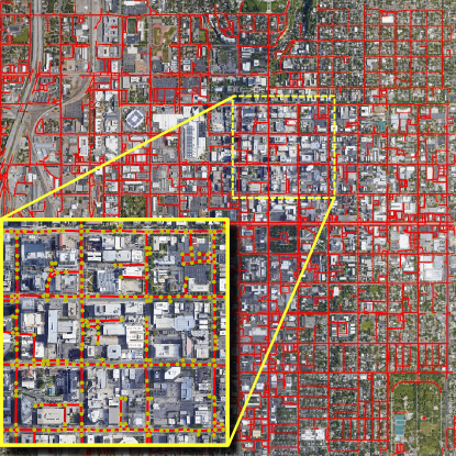
Figure 1: Result of our method on an image from the RoadTracer [5] test set. Our method regresses an entire graph without the need of pre or post-processing. This 8192x8192 pixel image was processed in 22 seconds on a single GPU, which is up to 91 times faster than previous approaches. The extracted graphs have a low complexity and retain good accuracy compared to existing works.

Vector-based maps are heavily used in Geographic Information Systems (GIS) such as online maps and navigation systems. The extraction of roads from overhead images has been, and mainly still is, performed by expert annotators. For a long time, handcrafted methods have been developed with the aim of reducing the burden of the annotators. However, they were not precise enough to replace them. Indeed, their outputs were imperfect and had a high dependence on user-adjustable parameters [31]. In recent years, the availability of large amounts of data [41], combined with the increase in compute capabilities, has led to a rise in the popularity of deep learning methods based on Convolutional Neural Networks [22]. Modern road extraction methods mostly fall into two kinds of approaches, each coming with its own drawbacks. The first kind [34, 53, 54, 7] relies on a pixel-based segmentation which is then converted to a graph using compute-intensive handcrafted algorithms that require a lot of manual tuning and can often yield partial graphs. The production of raster road masks using neural networks is a computationally expensive task in itself because of the large number of layers required to retrieve a segmentation that has the same resolution as the input image. Iterative graph construction methods are the second kind of deep learning based methods for road extraction [5, 29, 45, 30]. These approaches explore the map from an initial starting location using successive applications of a neural network on patches centered on the current point to predict the next-move. While having the advantage of directly inferring a graph, this is a very slow process. In addition, several starting locations may need be picked in order to cover the possible multiple connected components of the final graph.

Our approach aims to solve the aforementioned issues of current deep learning based methods by offering a fast and convenient way to extract roads from satellite or aerial images. Inspired by recent advances in neural networks for object detection [46], we design a fully convolutional detection head that learns to precisely locate multiple points of interest such as intersections, turns, and dead ends across the whole image in a single pass. Node features attached to these points are simultaneously regressed by this head, and fed to a Graph Neural Network (GNN) which predicts links between these points to form the final graph without requiring any post-processing. These networks are jointly trained end-to-end from ground truth road graphs, which are widely available from sources such as OpenStreetMap. We benchmark our method against state-of-the-art approaches on the RoadTracer [5] dataset and find that it is orders of magnitude faster than recent competing methods while retaining competitive accuracy. With the increasing interest in deep learning inference on embedded hardware, such as satellites or drones [3], our method, combined with recent advances in CNN and GNN quantization [8, 4], opens the possibility of on board in-flight road extraction, which could reduce ground computation and bandwidth needs by transmitting graphs instead of images.

The main contribution of our work is threefold. First, we propose a fast fully convolutional method for precise localisation of points of interest. Second, we design a Graph Neural Network for road link prediction. Third, we propose a performance-oriented architecture highly competitive against state-of-the art approaches.

2 Related Works

2.1 Convolutional Neural Networks

In recent works, Convolutional Neural Networks (CNN) such as VGG [44] or ResNet [14] which were originally used for image classification, are stripped of their final classifier and repurposed as fully convolutional feature extractors (often called backbones) for other computer vision tasks, such as semantic segmentation [33]. Object detection methods such as YOLO [39] or FCOS [46] have taken advantage of the fully convolutional nature of these backbones to design very fast single stage object detection neural networks, which infer bounding boxes and classes in a single forward pass and can be trained end-to-end, as opposed to two-stage approaches that perform these tasks separately. Single-stage architectures often follow a similar structure composed of a backbone which extracts features, a neck outputting feature representations at different scales [32], and several detection heads performing the final task.

2.2 Road Extraction

A large number of unsupervised methods have been developed for road graphs extraction. We refer the reader to recent extensive surveys on the subject for more information [30]. In this section, we focus on recent road extraction methods based on deep learning. Early deep learning based methods for road extraction were patch-based applications of fully connected neural networks [36]. However, most recent neural network-based methods proceed differently and can be sorted into two groups.

The first group of methods is based on pixel-level segmentation. Inspired by the success of FCN [33] and U-Net [40], these methods use a backbone as an encoder and learned upscaling as a decoder to retrieve a classification of individual pixels of an input image. In [53], residual connections are added to a U-Net to improve road predictions. D-LinkNet [54] adapts the LinkNet architecture to form a U-Net-like network and achieve better connectivity. DeepRoadMapper [34] use a ResNet-based[14] FCN to produce a segmentation which is then converted to a graph using thinning and an additional connection classifier. In [7], the authors improve the connectivity of extracted networks by jointly learning the segmentation and orientation of roads. All segmentation-based approaches have the drawback of relying on post-processing techniques to convert the predicted road pixels to a road graph. Thus, these methods are slow and the final graphs can lack connectivity.

The second kind of approaches iteratively construct a graph from an initial starting point by successive applications of a neural network for next move prediction around the center of an input patch. These methods are inspired by the way human annotators iteratively create road graphs. In [48], a network predicts which points from the border of the output patch are linked to the center point. RoadTracer [5] uses a CNN to predict the direction of the next move with a fixed step size. PolyMapper [29] uses a Recurrent Neural Network (RNN) guided by segmentation cues to predict the road topology and building polygons. VecRoad [45] implements a variable step size for next move prediction in order to achieve better alignment of intersections. DeepWindow [30] estimates the road direction along a center line regressed by a CNN using a Fourier spectrum analysis algorithm. While these methods have the advantage of outputting a road graph directly, they cannot guarantee the exploration of the whole map from a single starting location. The choice of initial starting locations is a hard problem in itself. Moreover, the repeated application of CNNs makes these approaches very slow.

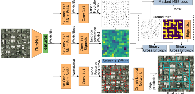
Figure 2: Our single-shot road graph extraction neural network. Features computed using a ResNet [14] backbone are fed to three branches. The junction prediction branch identifies cells which contain points of interest and is trained with binary cross-entropy. The offset prediction branch regresses the precise location of these points inside of the cells by outputting a two-dimensional vector field and is trained with a Mean Squared Error loss. Points selected by the junction and offset branch are paired with node features from a third branch and fed to a Graph Neural Network which predicts the presence of edges between pairs of points to create the final output.

2.3 Relational Inference and GNNs

Graph Neural Networks (GNNs) [42] are effective models for encoding interactions, and have recently been applied to link prediction [52], relational structure discovery, such as to model the dynamics of complex systems [18], and to the modeling of relational knowledge [43]. Kipf and Welling [19] proposed a graph autoencoder using a Graph Convolutional Network (GCN) encoder [20] and a simple dot-product decoder to model undirected networks and applied it to the link prediction task. Follow-up work [43] models different edge types in relational data using a graph neural network encoder and a decoder based on the DistMul [51] factorization. In [18] the authors propose a message-passing [12] encoder that alternates between the computation of node and edge features that can later be leveraged to predict the evolution of the system of interest several time steps in advance. The aforementioned models assume the ground-truth graph is partially known, or operate on the complete graph as an uninformative prior [18]. A parallel line of work is that of learning the unknown graph explicitly. The Dynamic Graph CNN model [50] proposes to dynamically build a graph by k-NN search in the feature space after each application of the EdgeConv operator also introduced in [50]. The approach has been extended in [16], where the authors address the question of the differentiable construction of a discrete graph using the recently proposed Gumbel Top-k trick [21] - a stochastic and differentiable relaxation of k-NN search - and decouple the construction of the graph and the learning of graph features amenable for downstream tasks. With the introduction of deeper architectures [24, 13] came increased interest for efficient implementations of GNNs, an issue relevant to our work as on-board processing of satellite images, such as for road graph extraction, is a pressing issue. [49] applied bucket-based quantization of matrix-matrix products to accelerate the GCN [20] operator. [4] proposed a general framework for binarizing graph neural networks and specifically introduced efficient binarized versions of the Dynamic EdgeConv operator [50] with real-world speed-ups on a low-power device.

3 Method

In this section, we present our method based on a fully convolutional head for regression of points of interest and a Graph Neural Network (GNN) for link prediction. An overview of our method is available in Figure 2.

3.1 General architecture

Our neural network architecture follows the trend of using a pre-trained CNN as a feature extractor (backbone). Most detection neural networks also use a Feature Pyramid Network (FPN) as a ”neck” that aggregates features from multiple scales. However, we chose not to use an FPN since satellite images have a fixed ground sampling distance and consequently, models that work on them are less vulnerable to changes in scale. Since we work at a single level of detail, we feed the output feature maps of the feature extractor directly to a single head. These changes allow us to save computation time and make the training process more streamlined. Indeed, we remove all ground truth bounding box assignment complications that arise when using multiple heads.

Each branch of our head is composed of three convolutional layers working on $N_{feat}$ feature maps. The first two branches are the junction-ness and offset branch, which form the point-of-interest detection model. The third branch is a node feature branch, which computes features that will be used to predict links between points detected by the ”point-of-interest” branch.

Let $H_{I},W_{I}$ be the dimensions of the input RGB image $I\in\mathbb{R}^{H_{I}\times W_{I}\times 3}$. With the ResNet-50 [14] backbone used in our experiments, the height and width $H,W$ of the input feature maps $F^{in}\in\mathbb{R}^{H\times W\times N_{in}}$ are 32 times smaller than the ones of $I$. This means that the final layers of our head have $H\times W$ output cells. In the case of an input image size of $512\times 512$ pixels, for example, we thus obtain 256 output cells, which can each regress the position of one point.

3.2 Point detection branch

Our point of interest detection branch, shown in Figure 2 is inspired by recent developments in single shot detection neural networks [46, 39], which regress a bounding box for each output ”cell” of a detection head, even if they do not necessarily contain an object. This allows object detection to be performed using very fast Fully Convolutional Networks. In [46], the notion of ”center-ness” is then introduced to filter out cells that do not belong to any object. These methods represent bounding boxes as four offsets relative to the center of the cell. We adapt this design to the regression of points of interest by outputting a ”junction-ness” score $J_{j}$ for each output cell $j$, as well as a two-dimensional vector $\mathbf{o}_{j}=[u_{j},v_{j}]\in[-0.5;0.5]^{2}$ representing the offset of the regressed point with respect to the center of its cell. A point $\mathbf{p}_{j}$ is detected in an output cell $j$ if $J_{j}>J_{thr}$, where $J_{thr}$ is the junction-ness detection threshold. We can retrieve the coordinates $(x_{j},y_{j})$ of $\mathbf{p}_{j}$ in the original input image:

$$x_{j}=\frac{u_{j}+X_{j}+0.5}{W}\cdot W_{I},y_{j}=\frac{v_{j}+Y_{j}+0.5}{H}\cdot H_{I}$$ (1)

where $(X_{j},Y_{j})$ are the coordinates of the cell $j$ in the output feature map $F^{out}$.

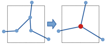
Figure 3: Node averaging which occurs when several ground truth points belong to the same output cell. The offset branch is thus trained to regress the centroid of these ground truth points.

3.3 Choice of input resolution

By design, our method is only able to find a single point of interest by output cell and is directly trained on ground truth annotations. However, depending on the dataset, and especially in very dense neighborhoods, several ground truth points may fall into the same cell. We chose that these points would effectively be merged into their centroid, while keeping incoming edges from outside of that cell linked to that new point, as shown on Figure 3. However, this situation should be avoided as much as possible, since it can shift intersections, and link close points that should not be linked (e.g. parallel roads). Images are often resized when being forwarded through a neural network, as a compromise between speed, memory and accuracy. In our case, the resizing ratio has to be chosen carefully according to the ground sampling distance (GSD) of the dataset and the density of ground truth annotations. To estimate the correct ratio for each dataset, we evaluate the average number of points in each positive cell over the whole dataset, at a wide range of ratios. This average should be as close to one as possible, in order to limit the effects of point merging. Figure 4 shows this average for the popular RoadTracer [5], SpaceNet3 [47] and Massachussetts roads [35] datasets.

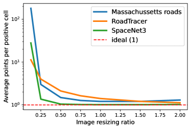
Figure 4: Average ground truth points per positive output cell at a range of image resizing ratios for 3 popular road extraction datasets. The ideal average is one, to prevent the collapse of neighboring nodes as much as possible.

3.4 Edge prediction

Once junctions have been extracted from the image, our task is to predict which ones are connected. We cast the problem as that of learning a latent graph. Starting with an initial prior connectivity estimation - i.e. a set of edges - $\mathcal{E}^{0}$, we aim at both inferring missing edges and discarding irrelevant ones.

Formally, let $j$ be one of the detected junctions. We denote by $X_{j}=F^{out}_{j}$ the corresponding features in the output feature map of the backbone, and $\mathbf{p}_{j}=(x_{j},y_{j})$ the 2D Cartesian coordinates of the junction in the input image, computed from the offset vectors.

Our method computes initial node embeddings

$$\mathbf{x}_{j}=f(X_{j},\mathbf{p}_{j}).$$ (2)

We choose the function $f$ to be either a 2D Convolutional Neural Network defining an additional node features branch of the network - responsible for dimensionality reduction and transformation of the raw image features - or the identity, the latter case leaving the task of transforming the raw image features to the GNN. We then perform several (e.g. three) message-passing iterations using the EdgeConv operator [50]:

$$\mathbf{e}^{(l)}_{ij} =\text{ReLU}\left(\bm{\theta}^{(l)}(\mathbf{x}^{(l-1)}_{j}-\mathbf{x}^{(l-1)}_{i})+\bm{\phi}^{(l)}\mathbf{x}^{(l-1)}_{i}\right)$$ (3)

$$=\text{ReLU}\left(\bm{\Theta}^{(l)}\tilde{\mathbf{X}}^{(l-1)}\right)$$ (4)

$$\mathbf{x}^{(l)}_{i} =\max_{j\in\mathcal{N}(i)}\mathbf{e}^{(l)}_{ij}$$ (5)

followed by Batch Normalization, where $\tilde{\mathbf{X}}^{(l-1)}=\left[\mathbf{x}^{(l-1)}_{i}\operatorname*{||}\mathbf{x}^{(l-1)}_{j}-\mathbf{x}^{(l-1)}_{i}\right]$, $\bm{\theta}$ and $\bm{\phi}$ are trainable weights, and $\bm{\Theta}$ their concatenation. The resulting increase in receptive field allows for connectivity patterns to be learned based on both local image and graph properties, and shared context across junctions.

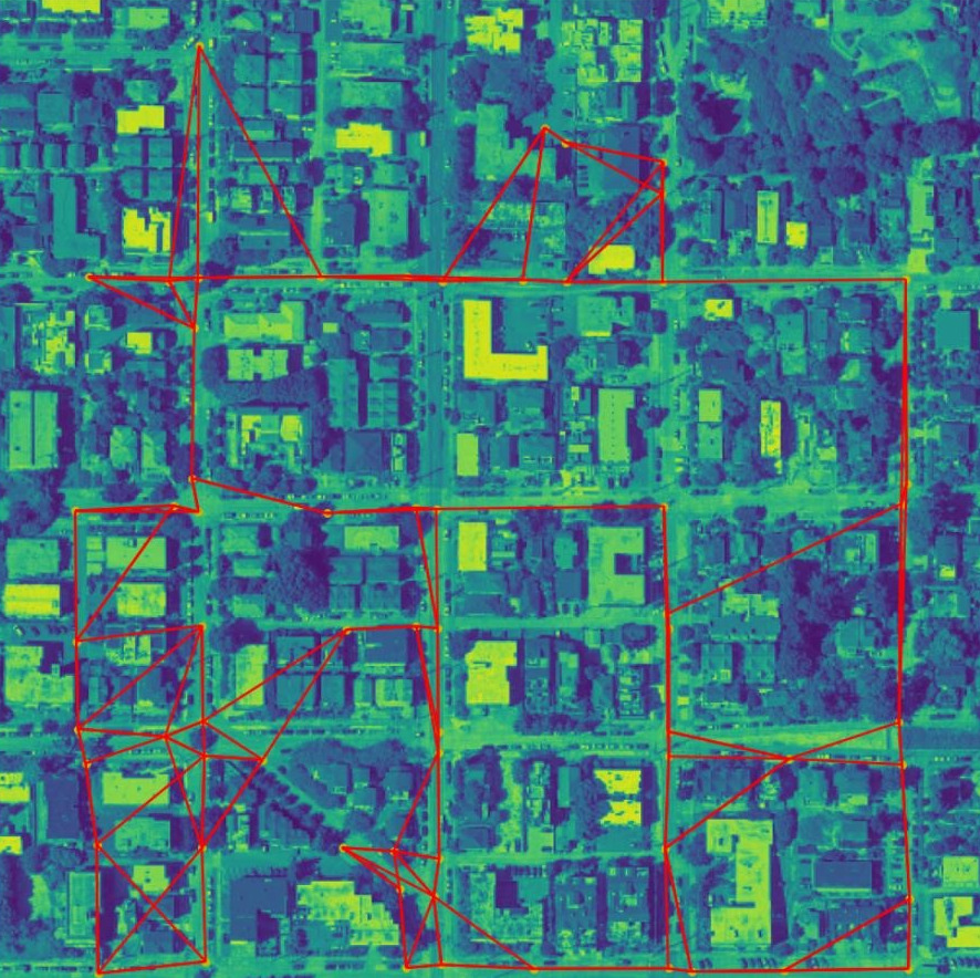
Figure 5: $k=4$-NN graph constructed in feature space on features learned by an additional node features head combined with an MLP edge classifier.

Finally, each possible edge is scored using a simple scoring function $g$ applied on the final node features of the graph. While we could opt to classify the edges based on the computed edge features $\mathbf{e}_{ij}$, performing message passing on a sparse graph (potentially built dynamically) is desirable for efficiency at both training and inference. We note

$$p_{ij}=\sigma(g(\mathbf{x_{i},x_{j}}))$$ (6)

the inferred probability that the edge $\mathbf{e}_{ij}$ exists, where $\sigma$ is the sigmoid function. In practice, we choose $g$ to be either a single bilinear layer, i.e.

$$g(\mathbf{x}_{i},\mathbf{x}_{j})=\mathbf{x}_{i}^{T}W_{g}\mathbf{x}_{j}$$ (7)

or a multi-layer MLP classifier (please refer to the appendix for more details and comparison with other decoders such as the dot product).

Connectivity estimation

Our choice of operator is motivated by the fact the connectivity is unknown, and therefore we may choose $\mathcal{E}^{0}$ to the set of edges of the complete graph (i.e. considering all possible connections between junctions), or introduce a sparse prior by building the graph dynamically by $k$-NN search in feature space. We also considered the case where the initial graph is complete, while subsequent iterations of message passing are done on dynamically inferred connectivity. Choosing $k=4$ is motivated by the observations that junctions with more than four incident roads are rare. To verify this intuition, we trained a model using a three-layer (2D convolutions followed by Batch Normalization and ReLU activations) node features head and an MLP classifier for each possible edge. The model was trained to convergence, and the four nearest neighbours graph was built on the output of the node features branch. The resulting graph is shown in Figure 5, and demonstrates that a high quality sparse initialization of the connectivity can be obtained in this manner.

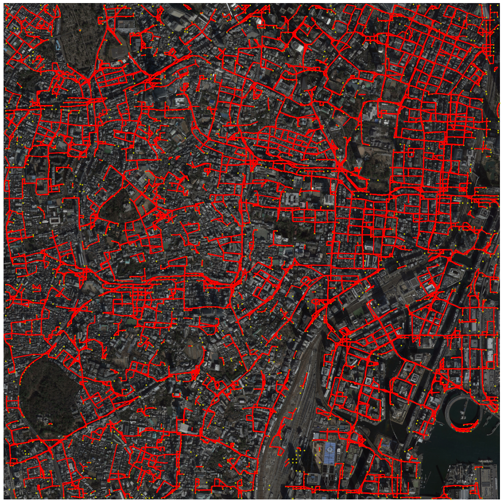
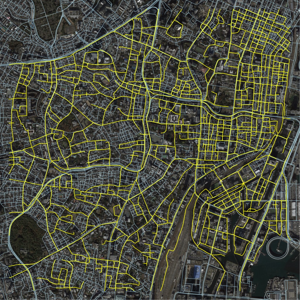
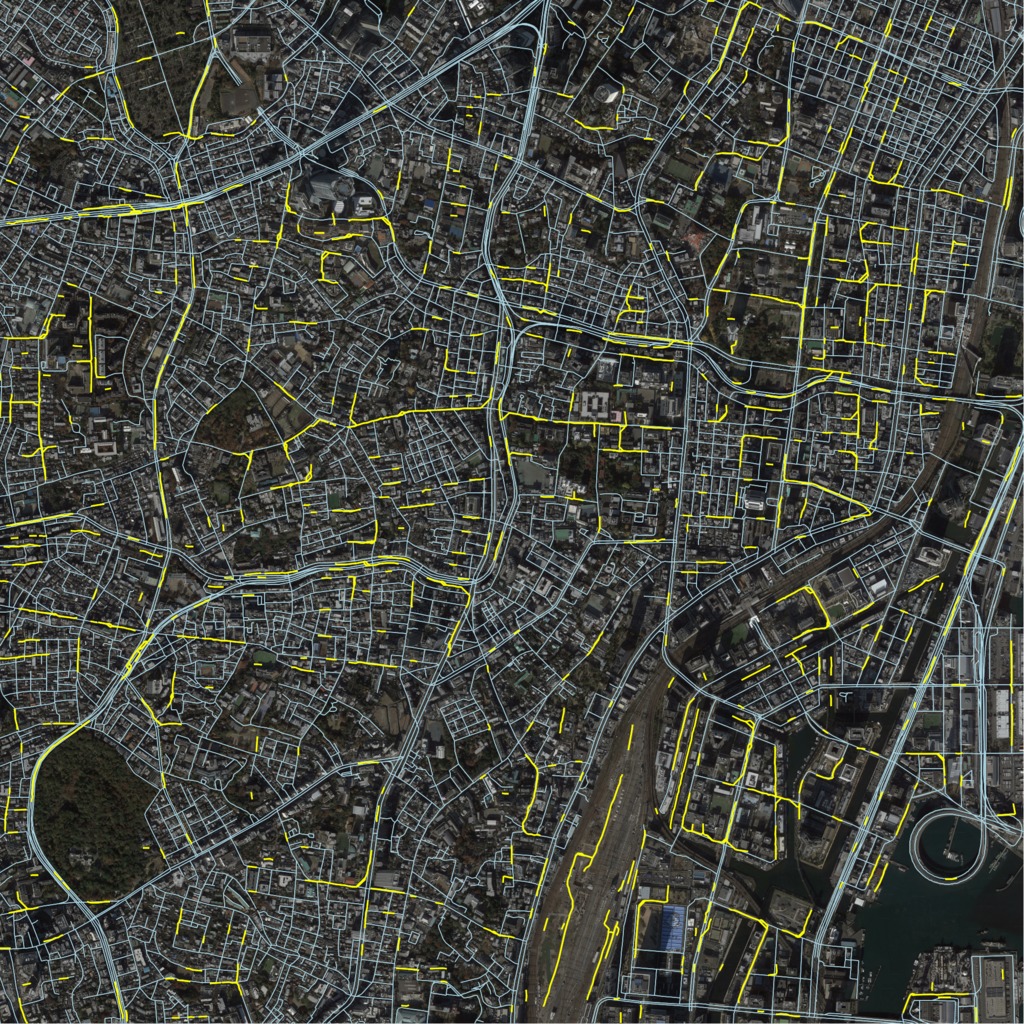
Figure 6: Comparison of our method (left) against an iterative method [5] (middle) and a segmentation based method [34] (right). Our method is able to find more roads in this challenging area of the RoadTracer test set, even in sections that are completely missed by other methods.

3.5 Loss function

To train our neural network our loss function is defined as a sum of three terms:

$$\mathcal{L}=\mathcal{L}_{\text{jun}}+\mathcal{L}_{\text{off}}+\mathcal{L}_{\text{edge}}$$ (8)

where $\mathcal{L}_{\text{jun}}$ and $\mathcal{L}_{\text{edge}}$ are the binary cross-entropy loss which we use to train our junction-ness branch and our edge prediction Graph Neural Network.

$\mathcal{L}_{\text{off}}$ is a Mean Squared Error offset loss masked with the positive junction predictions, which we use to train our offset regression branch. We define it as:

$$\mathcal{L}_{\text{off}}=\frac{1}{\sum\mathbbm{1}_{J_{i,j}>J_{thr}}}\sum_{i,j}\mathbbm{1}_{J_{i,j}>J_{thr}}(v_{i,j}-V_{i,j})^{2}$$ (9)

Where $V$ is the ground truth offset vector field. The mask is used so that the predictions of the offset branch are not conditionned to the presence of nodes.

3.6 Inference on large images

In our testing, we found that the output of the link prediction branch is tied to the original training resolution of the network. Thus, we did not obtain good results by directly inferring on a bigger image. Instead, we apply our network on large images using a sliding window of the same size as the training resolution, and accumulate the detected edges.

4 Experiments

In this section, we compare our method against other road extraction approaches on the widely-used RoadTracer dataset [5], which is composed of 35 training cities (180 images of 4096x4096 pixels) and 15 test cities of 8192x8192 pixels. The low number of training images, low ground sampling distance, high resolution and high annotation density of this dataset make it quite challenging.

4.1 Implementation details

According to the results shown in Figure 4, we choose a rescaling ratio of 0.5 as a good compromise between accuracy and speed. We implement our method in the Pytorch 1.9.1 [38] framework based on CUDA 11. We choose a ResNet-50 backbone (thus $N_{in}=2048$) and $N_{feat}=256$. We perform edge classification on the complete graph (other cases included in the appendix) using a three-layer GNN and a 2-layer MLP scoring function. We use basic data augmentation techniques such as random flips, and train our network on 512x512 pixel random crops for 2350 epochs, which took 24 hours on our system with a single Nvidia RTX 3090 GPU with 24GB of VRAM, an AMD Ryzen 9 3900X CPU and 64GB of RAM. We use the Adam [17] optimizer with a learning rate of $1e^{-3}$.

We also run performance benchmarks. All numbers were obtained on a computer with two Intel Cascade Lake 6248 20-core CPUs, 192GB of RAM, and four Nvidia Tesla V100 GPU with 16GB of VRAM. 10 CPU cores, a single GPU, and a quarter of the available memory were assigned to each run.

4.2 Qualitative results

Figure 6 shows qualitative results against an iterative method and a segmentation-based method. Our method is able to find a noticeably larger number of roads than RoadTracer [5] and DeepRoadMapper [34] in this challenging image. We can also notice that there are a few areas with low connectivity compared to RoadTracer. Indeed, since their network ”walks” through the entire regressed graph, it is inherently made of a single connected component. However, the result of RoadTracer is missing entire portions of the city (e.g. top left) because they are separated from the starting position by a highway that the network was not able to cross during its exploration. Our method does not suffer from such limitations. More qualitative results are available in Figure 1 and in appendix.

4.3 Quantitative evaluation

We follow the literature and use the three metrics defined in [45] to evaluate the accuracy of our network. P-F1 is a pixel-based F1 score obtained by comparing the rasterized output graph and ground truth. J-F1 is a junction-based F1 score based on local connectivity. APLS is the Average Path Length Similarity defined in the SpaceNet challenge [47] and is based on the comparison of shortest paths in the predicted graph and the ground truth.

The results of our testing are shown in Table 1. Our method achieves results which are competitive with DeepRoadMapper [34] and RoadTracer [5]. It is however outperformed by VecRoad [45]. Our intuition is that VecRoad sort of ”brute-forces” these metrics by regressing a lot more points and edges than our method, as shown in Section 4.5 and Table 3.

Method	P-F1	J-F1	APLS
DeepRoadMapper [34]	56.85	29.05	21.27
RoadTracer [5]	55.81	49.57	45.09
RoadCNN[5]	71.76	–	–
VecRoad[45]	72.56	63.13	64.59
Ours	57.2	39.23	46.93

Table 1: Accuracy metrics on the RoadTracer Dataset, evaluated using open source code from [45] and [5]. RoadCNN is a purely segmentation-based method implemented by [5], thus it only has a P-F1 score.

4.4 Performance benchmarks

Run-time is seldom mentioned in the road extraction literature, but it is a very important metric, especially as we move towards inference on edges devices. Thus, we benchmark the performance of our method against other recent approaches with open source code. We remove data loading and output times from all methods and thus only account for pre-processing, inference and post-processing steps of each algorithm. We provide average performance numbers for a single 8192x8192 test image from the RoadTracer [5] dataset, as well as numbers for the whole dataset (15 images), since some methods such as VecRoad [45] have optimizations for multiple-image inference. Our method can run on the whole dataset at once by performing the sliding window in batches, which is a bit faster.

Method	Type	Single image	Whole dataset
VecRoad [45]	Iterative	1902.5	8873.4
RoadTracer [5]	Iterative	579.4	8690.5*
DeepRoadMapper [34]	Seg.	1361.6	20423.4
RoadCNN [5]	Seg.	58.6	878.5
Ours	Graph	20.9	295.0

Table 2: Run-time in seconds on the RoadTracer Dataset. The single image score is averaged over the whole test set. Our method is the fastest by a large margin. *RoadTracer failed on some images, thus this number is extrapolated from the average.

The results of this experiment are shown in Table 2 and Figure 7. We observe that iterative methods are much slower because of the repeated forward passes required for next move estimation. Segmentation methods are not particularly fast as well, as the upscaling computation performed by a learned decoder is very compute intensive, and the extra post-processing steps required for graph conversion are slow. Our method is the fastest one by a large margin and offers a very good compromise between accuracy and speed. Indeed, it achieves similar APLS scores as RoadTracer [5] while running 27 times faster. Our approach also beats the APLS scores of DeepRoadMapper [34] by a large margin while running 65 times faster. It has lower accuracy scores than VecRoad [45], however it is 91 times faster. Our method could be made even faster by using a smaller and more efficient backbone, such as ResNet-18 [14] or DarkNet-53 [39].

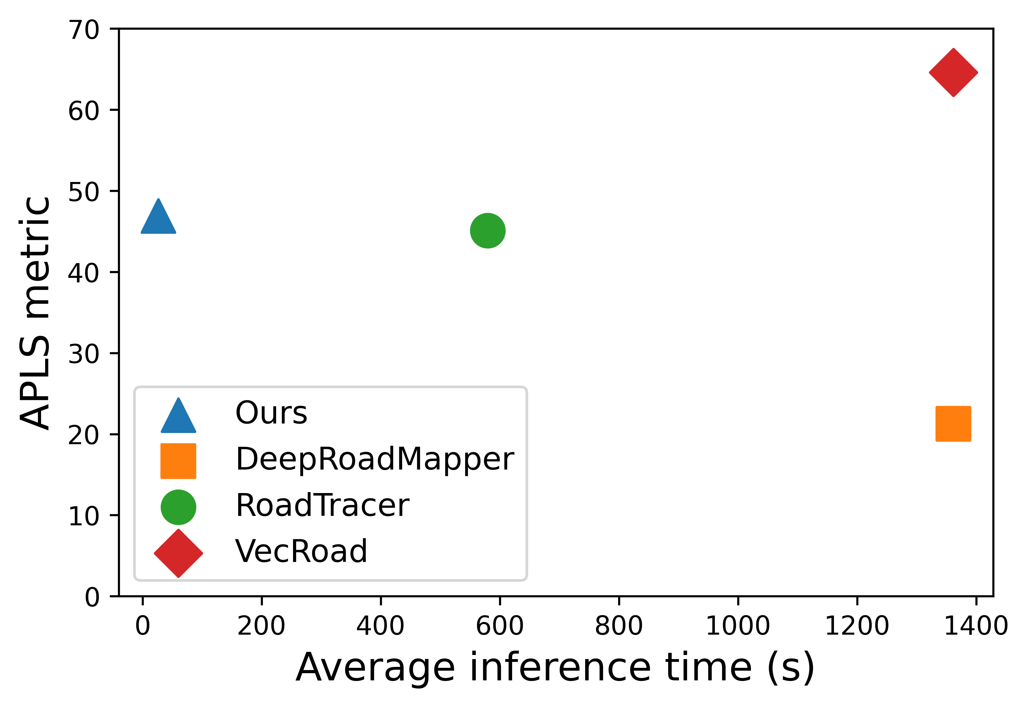
Figure 7: APLS metric with respect to inference time for our method, compared to state-of-the art approaches. Our method is the fastest and offers a very good compromise between accuracy and speed.

4.5 Graph complexity

Another interesting metric which is seldom mentioned in the road extraction literature is the notion of graph complexity. Graphs are a sparse representation and are meant to use a lot less storage space than masks. Most algorithms commonly used on graphs (e.g. shortest path algorithms) have a complexity which depends on the number of nodes and edges of the graph. Thus, offering accurate graphs with a low number of unnecessary nodes and edges is also beneficial in terms of run-time of subsequent applications. To evaluate the complexity of the graphs regressed by our method and compare it to other approaches, we propose a complexity score (lower is better) which is simply the total number of graph elements (nodes and edges) divided by the APLS score. We use the APLS because it seems to be the most popular metric. This score represents the compromise between the accuracy and compactness of graphs.

The results of this experiment are shown in Table 3. We observe that our method obtains the lower complexity compared to VecRoad [45] and DeepRoadMapper [34]. This is mainly due to our sparse approach to the regression of junctions, as shown by the average number of nodes. In Figure 8, we show the way our method finds an optimal representation of a neighborhood compared to the very high number of nodes and edges found by VecRoad [45].

Method	Nodes	Edges	Total	APLS	Complexity
VecRoad [45]	29620	61042	90662	64.59	1404
DRM [34]	6071	11963	18034	21.27	848
RoadTracer [5]	8263	17044	25306	45.09	561
Ours	4343	17273	21615	46.93	461

Table 3: Comparison of average graph complexity scores (Total elements divided by APLS. Lower is better). Nodes (resp. Edges) is the average number of nodes (resp. edges) in the output graphs over the whole RoadTracer test set. DRM = DeepRoadMapper. Our method achieves the lowest complexity compared to other approaches, which make it a good compromise between accuracy and compactness of graphs.

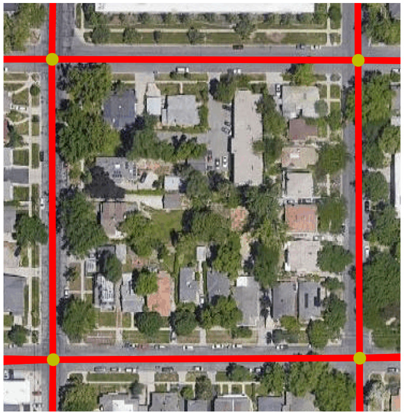
Figure 8: Exemple of the low complexity of the graphs inferred by our method (left) compared to VecRoad [45] (right). Our method finds an optimal 4-node representation of this simple neighborhood, whereas iterative methods tend to find overly complex representations. Having graphs with a low number of elements will save storage and speed up the computation of algorithms performed on these graphs, such as shortest path algorithms.

5 Limitations

Our method comes with some limitations. The first one, as said in previous sections, is the difficulty to work in very dense areas with lots of intersections. Since multiple intersections might fall into the same detection cell, our network will only be able to detect one of them, which can lead to shifted junctions. The second limitation is the inability to be trained on mask-based datasets such as DeepGlobe [9]. Our network can only be trained on graphs, and such data might not always be available. Finally, some long sections of road such as highways or bridges might lack points of interest since they do not have any junctions. Our network can miss these sections of road in the final graph as shown in Figure 9 and in some parts of Figure 1.

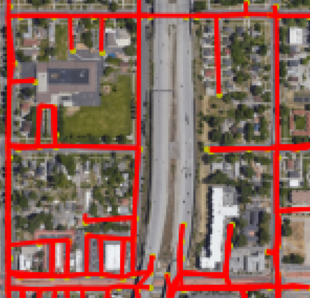
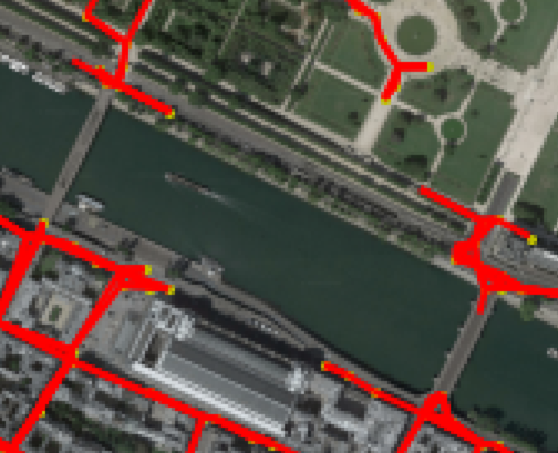
Figure 9: Examples of long sections of road (e.g. highways, bridges) without points of interest, which are occasionally missed by our method.

6 Conclusion

We proposed a novel architecture for single-shot extraction of road graphs from satellite images. Our method first predicts sparse interest points using an image CNN feature extractor as well as a junction detection head, and an offset regression head, trained jointly to identify candidate road intersections in a lower-resolution image and predict their position in the high-resolution image. We then combine the extracted image features and regressed point coordinates with a graph neural network to combine local and global information and infer the unknown graph structure. Our method combines aspects of graph learning and link prediction to score candidate connections between road junctions and infer the road graph. We demonstrate competitive performance with state of the art methods on three reference metrics while achieving significantly lower graph complexity and inference times (up to 91x faster than iterative models) compared to iterative and segmentation-based methods.

Even though the experimental validation of our approach was focused on road networks, our single-shot graph extraction framework can be applied to other types of problems. An example would be the extraction of blood vessels in medical images [10]. An interesting follow-up to road extraction could be to not only decide if edges exist or not in the final graph, but also infer edge attributes like road types, amount of traffic, or speed limits, as done in [11]. We also believe that our method could be adapted to tackle map update problems that have been presented in newly released datasets [6]. In addition, our method can further be combined with existing model compression techniques, both from the Euclidean and Geometric deep learning literature, to pave the way for on board single-shot extraction of road graphs on edge devices.

Appendix A Impact of choosing a smaller backbone

Feature extractors (backbones) come in different sizes to suit different kinds of performance targets. For example, some applications like edge computing might accept a reduction on accuracy in favor of faster inference time and higher throughput. In order to evaluate the impact of choosing a smaller backbone on our method, we take the network presented in the main text and replace the ResNet-50 backbone with ResNet-18.

Method	APLS	Single image time (s)
Ours (R18)	38.80	19.6
Ours (R50)	40.45	20.9

Table 4: Run-time in seconds on the RoadTracer Dataset. The single image score is averaged over the whole test set. Using a smaller backbone (R18) is slightly faster but causes a small drop in APLS.

The results of this experiment are presented in Table 4. We observe that using a ResNet-18 backbone is slightly faster but results in a slightly lower APLS score. This means that our method works with smaller backbones and thus can be used on a variety of low power devices, especially ones that have a low amount of memory, such as the Nvidia Jetson family of devices.

Appendix B Impact of edge detection threshold

In this section, we study the impact of the edge detection threshold, which can be freely chosen between 0 and 1. To do this, we compute the three main accuracy metrics for a range of thresholds varying between 0 and 0.5, using our main model. Setting a high detection threshold favors the Precision of edges, while setting a low threshold favors the Recall. Figure 10 shows the results of this experiment. We observe that the P-F1 (pixel metric) and APLS are better when detecting more edges, while the J-F1 (junction metric) is slightly better when detecting fewer edges. This makes sense as the J-F1 is based on having the correct number of edges for each junction, while the APLS should benefit from more path options. The P-F1 may be higher at low thresholds simply because we find more road pixels. This experiment shows that finding and setting an appropriate edge threshold for each model is important in order to obtain the best accuracy and the best compromise between the three metrics.

Figure 10: J-F1, P-F1 and APLS scores for our main model, at a range of edge detection thresholds.

Appendix C On the J-F1 metric

As previously said in the Method and Limitations sections of our main text, our method is only able to find a single point-of-interest per output cell, which can lead to merged junctions in the output graph. In addition, as seen in the Experiments section of the main text, our method will inherently find a lower number of junctions since it is tailored towards the extraction of a sparse graph. Since the J-F1 score is based on a matching of junctions within a certain radius, we believe that these design choices significantly affect this metric, which leads to our method scoring lower than some other approaches.

#	Pre-trained	Init Graph	GNN	Classifier	Raw feat	Wait	Train $j_{thr}$	J-F1	P-F1	APLS	Sum
1	✓	Baseline	✗	Bilinear				40.33	55.93	43.95	140.21
2		Baseline	✗	Bilinear				36.03	53.87	41.64	131.54
3		Baseline	✗	Bilin small				32.24	50.4	36.11	118.75
4	✓	Baseline	✗	MLP				36.92	53.43	41.17	131.53
5		Baseline	✗	MLP				35.46	56.03	45.35	136.84
6	✓	Complete	EdgeConv	Bilinear				37.69	56.04	45.39	139.13
7*	✓	Complete	EdgeConv	MLP				39.23	57.2	46.93	143.36
8	✓	Dynamic	EdgeConv	Bilinear				35.63	56.29	46.04	137.96
9	✓	Dynamic	EdgeConv	Bilinear			0.3	37.90	55.5	43.68	137.08
10	✓	Dynamic	EdgeConv	Bilinear	✓			37.32	52.07	38.51	127.91
11	✓	Dynamic	EdgeConv	Bilinear	✓		0.3	37.92	52.37	40.27	130.55
12	✓	Dynamic	EdgeConv	MLP				38.44	56.7	46.21	141.35
13	✓	Dynamic	EdgeConv	MLP	✓			34.95	53.75	41.57	130.27
14	✓	Dynamic	EdgeConv	MLP	✓		0.3	35.54	56.5	45.91	137.95
15	✓	kNN-4	EdgeConv	Bilinear				37.30	54.25	42.28	133.83
16	✓	kNN-4	EdgeConv	MLP				37.41	57.54	48.71	143.66
17	✓	Complete	DeepGCN	MLP	✓			37.17	55.43	42.59	135.19
18	✓	Complete	1 Conv + DeepGCN	MLP				38.35	57.11	47.12	142.58
19	✓	Complete	4 Conv + DeepGCN	MLP				37.89	57.71	48.84	144.44
20		Dynamic	EdgeConv	Bilinear				34.52	50.74	35.52	120.78
21		Dynamic	EdgeConv	Bilinear	✓	30		33.23	46.26	30.71	110.20
22		Dynamic	EdgeConv	Bilinear		30		32.03	50.94	37.31	120.28
23		Dynamic	EdgeConv	Bilinear	✓	30	0.3	36.89	49.02	32.13	118.04
24		Dynamic	EdgeConv	MLP				36.35	56.31	45.55	138.21
25		Dynamic	EdgeConv	MLP		30		36.54	55.72	43.97	136.22
26		Dynamic	EdgeConv	MLP		30	0.3	34.32	55.41	45.65	135.38
27		Dynamic	EdgeConv	MLP		10	0.3	35.36	54.96	44.44	134.76
28		Dynamic	EdgeConv	MLP	✓	30	0.3	34.48	55.02	42.15	131.65
29		Dynamic	EdgeConv	MLP	✓	30		35.73	54.9	41.91	132.54
30		Dynamic	EdgeConv	MLP	✓	10	0.3	34.90	56.03	44.60	135.54

Table 5: Variations on our model. Pre-trained = use of pre-trained ResNet and junctionness/offset branches for faster training. Raw feat = GNN applied directly to ResNet features (no node feature convolutions). Wait = Number of epochs where only the junction-ness and offset branches are trained before training the edge branch (default: 0). Train $j_{thr}$ = junction-ness threshold used during training (default: 0.5). Sum = J-F1 + P-F1 + APLS. *variation presented in the main text

Appendix D GNN model choices and ablation study

In this section, we perform a comparative study of different design decisions for the GNN portion of the model.

We compare the following choices for the construction of the road graph:

1. Using the complete graph as the supporting graph for each GNN layer and treating the problem as a pure edge classification task

2. Initializing the road graph by $k$-NN search (k = 4) on the output of the node feature branch (dim = 256) to which we concatenate the Cartesian coordinates of the junctions (dim = 2)

3. Dynamic construction of the graph at each layer by $k$-NN search (k = 4) on the layer’s input (i.e., as described in point 2 for the first layer, and on the output features of the previous layer for subsequent layers)

We also compare two choices of edge scoring function:

1. A 2-layer MLP ($\text{FC}(256)\rightarrow\text{FC}(256)$ where FC($N$) denotes a fully-connected layer with $N$ output features)

2. A $256\times 256\times 1$ bilinear layer

We use a three-layer graph neural network based on the EdgeConv operator with BatchNormalization and ReLU activations. We parameterize the EdgeConv operators each with a linear layer with 256 output features. We also report the results of baseline models trained without graph convolutions.

Finally, we compare the 3-layer EdgeConv networks with DeepGCNs [25, 26] using the Generalized Graph Convolution (GENConv) operator [26], layer normalization [2] and ReLU activations. We apply the DeepGCN layers sequentially on:

1. The raw image features produced by the backbone (DeepGCN)

2. The output of one convolutional layer in the node feature branch (1 Conv + DeepGCN)

3. The output of 4 convolutional layers in the node feature branch (4 Conv + DeepGCN) as for the EdgeConv-based models

In case (1) we used 7 layers of (GENConv $\rightarrow$ LayerNorm $\rightarrow$ ReLU), in case (2) we used 6 layers, and in case (3) we used 3 layers, so as to keep model capacity comparable with the EdgeConv models applied on the full node feature branch. We applied the DeepGCNs on the complete graphs only.

For each of these experiments, we report the J-F1, P-F1 and APLS metrics at the edge threshold that maximizes their sum. Table 5 shows the results of these experiments. To enable faster experimentation, we initialized some of the models using the pre-trained weights of a ”Baseline MLP” model trained on the complete graph, such models are denoted by a checkmark in the ”Pre-trained” columns of Table 5.

We can draw the following conclusions from the experimental results shown:

• The baseline with the bilinear classifier outperforms the baseline with a 2-layer MLP, which is expected since it has a much larger number of parameters. While the improvement is noticeable, the model loses compactness and efficiency.

• All three constructions of the graph (complete, static $k$-NN and fully dynamic) are able to perform well and to outperform the MLP and the Bilinear baseline. Notably, the models that combine a GNN with an MLP classifier outperformed the ones with the same GNNs but a bilinear classifier (scoring function). The entire GNN adds fewer parameter than changing the MLP for a bilinear layer, and yet can bring larger performance deltas, which further motivates our choice of using an MLP scoring function.

• The best performing GNN with the EdgeConv operator used a fixed $4$-NN graph support for message passing (but still scored all possible edges for the final graph). However, choosing the right value of $k$ adds another element to hyperparameter tuning of the model and comes at the disadvantage of reduced robustness to cases where images have no junctions to detect (e.g. satellite images of large bodies of water such as lakes). We therefore chose to report the performance of the simpler model in the main text, while showcasing that sparse graph priors may indeed lead to better road graph reconstructions.

• Getting rid of the node features branch reduces the number of trainable parameters but appears to be detrimental to the performance in most cases. Experiments with deeper GNNs applied directly on the output of the backbone showed increased performance compared to shallower GNNs, although the graph construction differs (l. 14, 17)

• Compared to 3-layer EdgeConv networks on the complete graphs, 3-layer DeepGCNs applied following either a 1-layer or 4-layer node feature branch performed better. These models also outperformed the dynamic graph models and the 3-layer EdgeConv applied on a sparse $4$-NN graph (by a slimmer margin in the latter case). The DeepGCNs applied on raw features outperformed some of the shallower models trained with a node feature branch, but did not match the best performing models.

• All DeepGCNs outperformed the MLP baseline, which indicates that, keeping the edge scoring function the same, replacing all (DeepGCN, l. 17)or most (1 Conv + DeepGCN, l. 18)2D convolutions with graph convolutions leads to increased performance compared to a model that only uses 2D convolutions.

Deep Graph Convolutional Networks

We suspect the last two points are due to two effects: first, 2D convolutions can be seen as special cases of graph convolutions applied to the 2D lattice graph while enforcing translation equivariance; their inductive bias is well suited to the processing of images. In contrast, we applied the GNNs (EdgeConv or DeepGCN) on the (dynamic or complete) graphs of detected junctions, which means the GNNs do not have access to the neighboring pixel’s context whereas the 2D Euclidean convolutions do. We believe this contributes to the reduced performance of all graph-convolutional models compared to models that combine 2D convolutions and graph convolutions. Additionally, the higher performance of the graph convolution models compared to only using 2D convolutions - especially on the APLS metric - show the contribution of the graph-based models.

Regarding the relative performance of DeepGCNs compared to shallower EdgeConv models, the graphs extracted from the images are small: they have at most $16\times 16=256$ nodes and $(256)*(256-1)/2=32640$ edges. The increase in receptive field that comes with deeper models will lose effectiveness once the entire graph is covered at a given layer. Furthermore, the experiments we report with DeepGCNs in Table 5 are done using the complete graph as support. Messages from each node reach all other nodes in a single iteration, which reduces the benefits one can glean from using deeper models, and makes the GNNs more susceptible to the smoothing problem [28]. We therefore decided to report results using shallow GNNs using the EdgeConv operator which is well suited to learning edge features and to learning on dynamic graphs. Further work will investigate using DeepGCNs on sparse graphs as well as on graphs built on larger images.

Junctionness threshold

In addition to the ablation study, we evaluated the impact of the junction-ness threshold $j_{thr}$ used during training. Lowering this threshold seems to have a positive impact on the three metrics. Our intuition is that when the junction-ness threshold is lower, the subsequent GNN is presented with more nodes and a larger number of possible edges for each image, and is thus trained better and faster.

Appendix E Other uses of our method

Our method is generic in the sense that it could be used for applications other than road extraction. In fact, it could be suitable for any image to 2D graph application. For example, our method could be used for blood vessel extraction as done in [48]. Another example is the polygonal extraction of buildings in aerial images. Just like for road extraction, existing methods either rely on an iterative process [29] or on post-processing of a pixel-based segmentation [27]. Thus, our method is able to provide the same advantages in this task as for road extraction. Figure 11 shows an example of building extraction using our method.

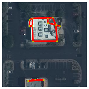
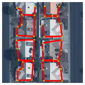
Figure 11: Our method can be used for other tasks, such as building extraction. This example is taken from the CrowdAI Mapping Challenge dataset [37]

Appendix F Qualitative results

Figures 12 and 13 show more qualitative results on cities from the RoadTracer test set. Our method is able to find more roads than RoadTracer [5] and DeepRoadMapper [34]. Some roads and highways that cannot be accessed easily by iterative approaches are found by our method. Our graphs also seem to have a better connectivity than the ones found by the segmentation-based method.

Appendix G Environmental impact statement

While the focus of our work is to create efficient neural networks that are able to run on very low power devices, we cannot help but notice that these networks are still created and trained using power-hungry multi-GPU machines and wonder about the environmental impact. For this paper, we tracked the number of GPU hours used and use that to estimate its global environmental footprint and publish these estimations, as recommended in [15, 1, 23].

In order to run the experiments required for our main results and ablation study, we have used 1572 GPU hours on Nvidia Tesla V100 GPUs, which are rated for a power consumption of 300W. This, not counting CPUs, cooling, PSU efficiency, storage of datasets and results, as well as different trials or hyper-parameter searches on workstations, amounts to 471,6kWh. Since the carbon intensity of our electricity grid is 10 gCO2/kWh, we estimate an emission of 4716 gCO2, which is equivalent to 39.17 km traveled by car according to [1].

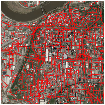
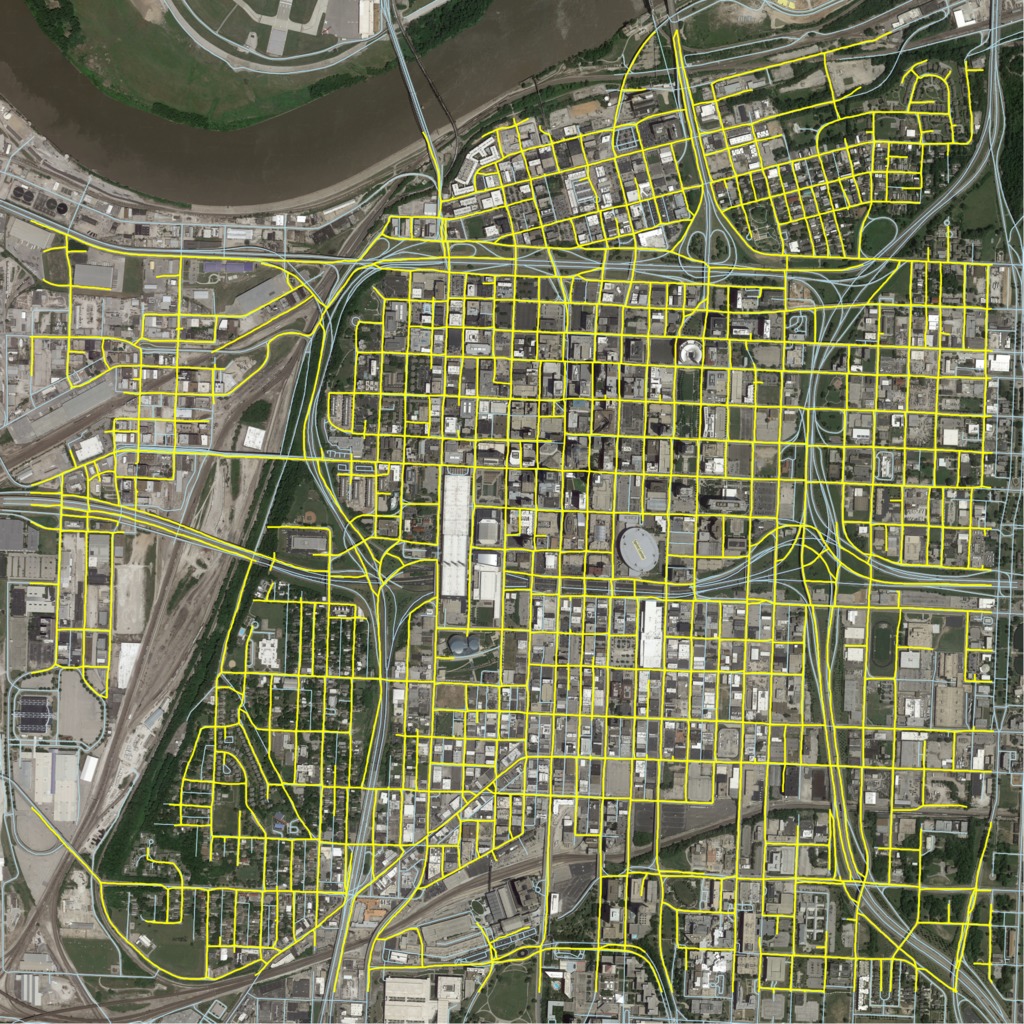
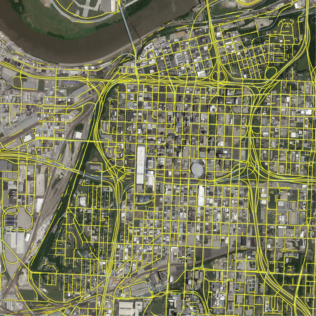
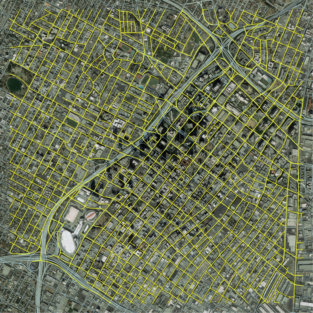
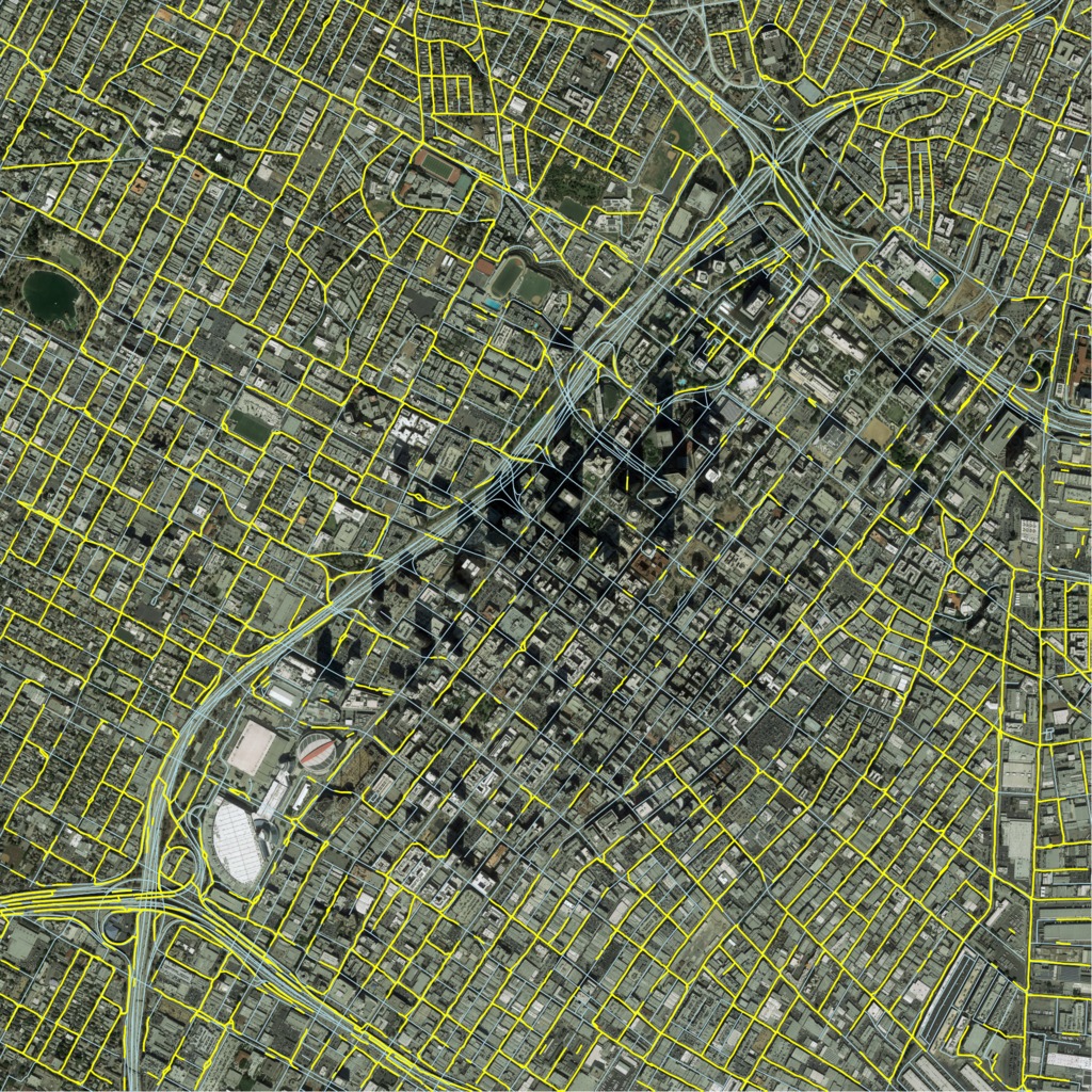
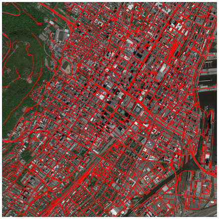
Figure 12: More qualitative results of our method (left) compared to RoadTracer [5] (middle) and DeepRoadMapper [34] (right), on the RoadTracer test set.

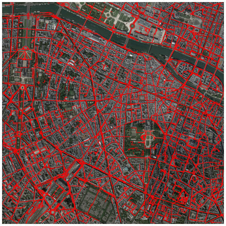
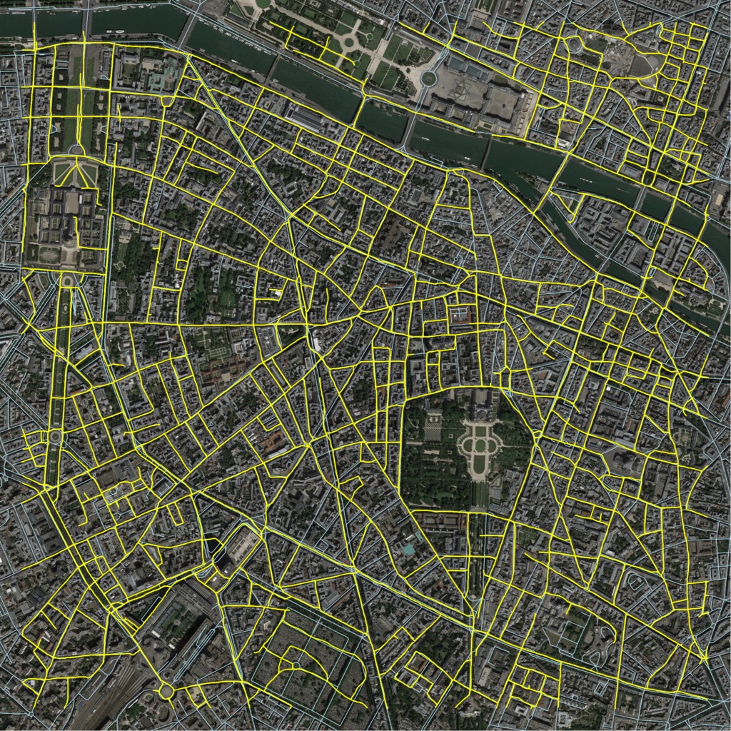
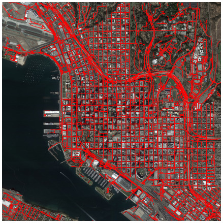
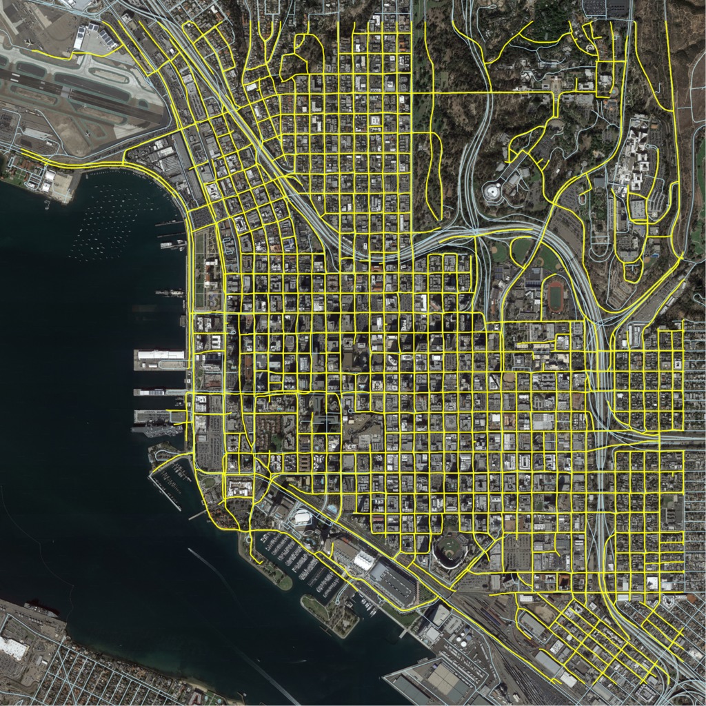
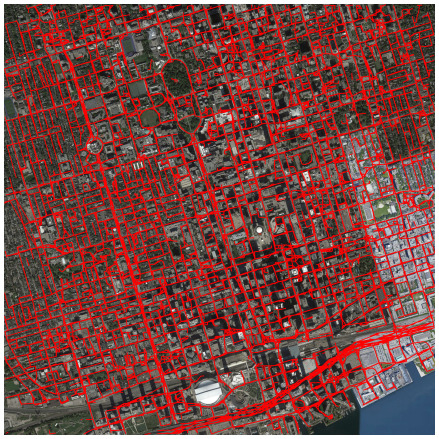
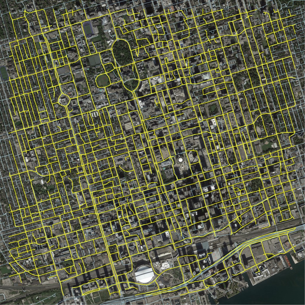
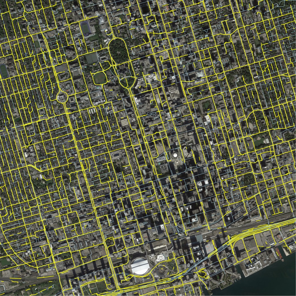
Figure 13: More qualitative results of our method (left) compared to RoadTracer [5] (middle) and DeepRoadMapper [34] (right), on the RoadTracer test set.

References

- [1] Lasse F Wolff Anthony, Benjamin Kanding, and Raghavendra Selvan. Carbontracker: Tracking and predicting the carbon footprint of training deep learning models. arXiv:2007.03051, 2020.
- [2] Jimmy Lei Ba, Jamie Ryan Kiros, and Geoffrey E Hinton. Layer normalization. arXiv preprint arXiv:1607.06450, 2016.
- [3] Gaétan Bahl, Lionel Daniel, Matthieu Moretti, and Florent Lafarge. Low-power neural networks for semantic segmentation of satellite images. In ICCV Workshops, 2019.
- [4] Mehdi Bahri, Gaétan Bahl, and Stefanos Zafeiriou. Binary graph neural networks. In CVPR, 2021.
- [5] Favyen Bastani, Songtao He, Sofiane Abbar, Mohammad Alizadeh, Hari Balakrishnan, Sanjay Chawla, Sam Madden, and David DeWitt. Roadtracer: Automatic extraction of road networks from aerial images. In CVPR, 2018.
- [6] Favyen Bastani and Samuel Madden. Beyond road extraction: A dataset for map update using aerial images. In ICCV, 2021.
- [7] Anil Batra, Suriya Singh, Guan Pang, Saikat Basu, CV Jawahar, and Manohar Paluri. Improved road connectivity by joint learning of orientation and segmentation. In CVPR, 2019.
- [8] Adrian Bulat and Georgios Tzimiropoulos. Xnor-net++: Improved binary neural networks. arXiv preprint arXiv:1909.13863, 2019.
- [9] Ilke Demir, Krzysztof Koperski, David Lindenbaum, Guan Pang, Jing Huang, Saikat Basu, Forest Hughes, Devis Tuia, and Ramesh Raskar. Deepglobe 2018: A challenge to parse the earth through satellite images. In CVPR Workshops, 2018.
- [10] Muhammad Moazam Fraz, Paolo Remagnino, Andreas Hoppe, Bunyarit Uyyanonvara, Alicja R Rudnicka, Christopher G Owen, and Sarah A Barman. Blood vessel segmentation methodologies in retinal images–a survey. Computer methods and programs in biomedicine, 108(1), 2012.
- [11] Zahra Gharaee, Shreyas Kowshik, Oliver Stromann, and Michael Felsberg. Graph representation learning for road type classification. Pattern Recognition, 120, 2021.
- [12] Justin Gilmer, Samuel S Schoenholz, Patrick F Riley, Oriol Vinyals, and George E Dahl. Neural message passing for quantum chemistry. In ICML, 2017.
- [13] Shunwang Gong, Mehdi Bahri, Michael M Bronstein, and Stefanos Zafeiriou. Geometrically principled connections in graph neural networks. In CVPR, 2020.
- [14] Kaiming He, Xiangyu Zhang, Shaoqing Ren, and Jian Sun. Deep residual learning for image recognition. In CVPR, 2016.
- [15] Peter Henderson, Jieru Hu, Joshua Romoff, Emma Brunskill, Dan Jurafsky, and Joelle Pineau. Towards the systematic reporting of the energy and carbon footprints of machine learning. Journal of Machine Learning Research, 21(248), 2020.
- [16] Anees Kazi, Luca Cosmo, Nassir Navab, and Michael Bronstein. Differentiable graph module (dgm) for graph convolutional networks. arXiv preprint arXiv:2002.04999, 2020.
- [17] Diederik P Kingma and Jimmy Ba. Adam: A method for stochastic optimization. arXiv preprint arXiv:1412.6980, 2014.
- [18] Thomas Kipf, Ethan Fetaya, Kuan-Chieh Wang, Max Welling, and Richard Zemel. Neural relational inference for interacting systems. In ICML, 2018.
- [19] Thomas N Kipf and Max Welling. Variational graph auto-encoders. arXiv preprint arXiv:1611.07308, 2016.
- [20] Thomas N Kipf and Max Welling. Semi-Supervised Classification with Graph Convolutional Neural Networks. In ICLR, 2017.
- [21] Wouter Kool, Herke Van Hoof, and Max Welling. Stochastic beams and where to find them: The gumbel-top-k trick for sampling sequences without replacement. In ICML, 2019.
- [22] Alex Krizhevsky, Ilya Sutskever, and Geoffrey E Hinton. Imagenet classification with deep convolutional neural networks. NeurIPS, 2012.
- [23] Loïc Lannelongue, Jason Grealey, and Michael Inouye. Green algorithms: Quantifying the carbon emissions of computation. arXiv:2007.07610, 2020.
- [24] Guohao Li, Matthias Muller, Ali Thabet, and Bernard Ghanem. DeepGCNs: Can GCNs go as deep as CNNs? In ICCV, 2019.
- [25] Guohao Li, Matthias Muller, Ali Thabet, and Bernard Ghanem. Deepgcns: Can gcns go as deep as cnns? In ICCV, 2019.
- [26] Guohao Li, Chenxin Xiong, Ali Thabet, and Bernard Ghanem. Deepergcn: All you need to train deeper gcns. arXiv preprint arXiv:2006.07739, 2020.
- [27] Muxingzi Li, Florent Lafarge, and Renaud Marlet. Approximating shapes in images with low-complexity polygons. In CVPR, 2020.
- [28] Qimai Li, Zhichao Han, and Xiao Ming Wu. Deeper insights into graph convolutional networks for semi-supervised learning. In 32nd AAAI Conference on Artificial Intelligence, AAAI 2018, 2018.
- [29] Zuoyue Li, Jan Dirk Wegner, and Aurélien Lucchi. Topological map extraction from overhead images. In ICCV, 2019.
- [30] Renbao Lian and Liqin Huang. Deepwindow: Sliding window based on deep learning for road extraction from remote sensing images. IEEE Journal of Selected Topics in Applied Earth Observations and Remote Sensing, 13, 2020.
- [31] Renbao Lian, Weixing Wang, Nadir Mustafa, and Liqin Huang. Road extraction methods in high-resolution remote sensing images: A comprehensive review. IEEE Journal of Selected Topics in Applied Earth Observations and Remote Sensing, 13, 2020.
- [32] Tsung-Yi Lin, Piotr Dollár, Ross Girshick, Kaiming He, Bharath Hariharan, and Serge Belongie. Feature pyramid networks for object detection. In CVPR, 2017.
- [33] Jonathan Long, Evan Shelhamer, and Trevor Darrell. Fully convolutional networks for semantic segmentation. In CVPR, 2015.
- [34] Gellert Mattyus, Wenjie Luo, and Raquel Urtasun. Deeproadmapper: Extracting road topology from aerial images. ICCV, 2017.
- [35] Volodymyr Mnih. Machine learning for aerial image labeling. University of Toronto (Canada), 2013.
- [36] Volodymyr Mnih and Geoffrey E. Hinton. Learning to detect roads in high-resolution aerial images. Lecture Notes in Computer Science (including subseries Lecture Notes in Artificial Intelligence and Lecture Notes in Bioinformatics), 6316 LNCS, 2010.
- [37] Sharada Prasanna Mohanty, Jakub Czakon, Kamil A Kaczmarek, Andrzej Pyskir, Piotr Tarasiewicz, Saket Kunwar, Janick Rohrbach, Dave Luo, Manjunath Prasad, Sascha Fleer, et al. Deep learning for understanding satellite imagery: An experimental survey. Frontiers in Artificial Intelligence, 3, 2020.
- [38] Adam Paszke, Sam Gross, Francisco Massa, Adam Lerer, James Bradbury, Gregory Chanan, Trevor Killeen, Zeming Lin, Natalia Gimelshein, Luca Antiga, Alban Desmaison, Andreas Kopf, Edward Yang, Zachary DeVito, Martin Raison, Alykhan Tejani, Sasank Chilamkurthy, Benoit Steiner, Lu Fang, Junjie Bai, and Soumith Chintala. Pytorch: An imperative style, high-performance deep learning library. In H. Wallach, H. Larochelle, A. Beygelzimer, F. d'Alché-Buc, E. Fox, and R. Garnett, editors, NeurIPS. 2019.
- [39] Joseph Redmon, Santosh Divvala, Ross Girshick, and Ali Farhadi. You only look once: Unified, real-time object detection. In CVPR, 2016.
- [40] Olaf Ronneberger, Philipp Fischer, and Thomas Brox. U-net: Convolutional networks for biomedical image segmentation. In International Conference on Medical image computing and computer-assisted intervention, 2015.
- [41] Olga Russakovsky, Jia Deng, Hao Su, Jonathan Krause, Sanjeev Satheesh, Sean Ma, Zhiheng Huang, Andrej Karpathy, Aditya Khosla, Michael Bernstein, et al. Imagenet large scale visual recognition challenge. IJCV, 115(3), 2015.
- [42] Franco Scarselli, Marco Gori, Ah Chung Tsoi, Markus Hagenbuchner, and Gabriele Monfardini. The graph neural network model. IEEE transactions on neural networks, 20(1), 2009.
- [43] Michael Schlichtkrull, Thomas N Kipf, Peter Bloem, Rianne Van Den Berg, Ivan Titov, and Max Welling. Modeling relational data with graph convolutional networks. In European semantic web conference. Springer, 2018.
- [44] Karen Simonyan and Andrew Zisserman. Very deep convolutional networks for large-scale image recognition. arXiv preprint arXiv:1409.1556, 2014.
- [45] Yong-Qiang Tan, Shang-Hua Gao, Xuan-Yi Li, Ming-Ming Cheng, and Bo Ren. Vecroad: Point-based iterative graph exploration for road graphs extraction. In CVPR, 2020.
- [46] Zhi Tian, Chunhua Shen, Hao Chen, and Tong He. Fcos: Fully convolutional one-stage object detection. In ICCV, 2019.
- [47] Adam Van Etten, Dave Lindenbaum, and Todd M Bacastow. Spacenet: A remote sensing dataset and challenge series. arXiv preprint arXiv:1807.01232, 2018.
- [48] Carles Ventura, Jordi Pont-Tuset, Sergi Caelles, Kevis Kokitsi Maninis, and Luc Van Gool. Iterative deep learning for road topology extraction. BMVC, 2018.
- [49] Junfu Wang, Yunhong Wang, Zhen Yang, Liang Yang, and Yuanfang Guo. Bi-GCN: Binary Graph Convolutional Network. In CVPR, 2021.
- [50] Yue Wang, Yongbin Sun, Ziwei Liu, Sanjay E Sarma, Michael M Bronstein, and Justin M Solomon. Dynamic Graph CNN for Learning on Point Clouds. ACM Trans. Graph., 38(5), oct 2019.
- [51] Bishan Yang, Wen-tau Yih, Xiaodong He, Jianfeng Gao, and Li Deng. Embedding entities and relations for learning and inference in knowledge bases. arXiv preprint arXiv:1412.6575, 2014.
- [52] Muhan Zhang and Yixin Chen. Link Prediction Based on Graph Neural Networks. In S Bengio, H Wallach, H Larochelle, K Grauman, N Cesa-Bianchi, and R Garnett, editors, NeurIPS, 2018.
- [53] Zhengxin Zhang, Qingjie Liu, and Yunhong Wang. Road extraction by deep residual u-net. IEEE Geoscience and Remote Sensing Letters, 15(5), 2018.
- [54] Lichen Zhou, Chuang Zhang, and Ming Wu. D-linknet: Linknet with pretrained encoder and dilated convolution for high resolution satellite imagery road extraction. In CVPR Workshops, 2018.