Contextualized Spatio-Temporal Contrastive Learning with Self-Supervision

Abstract

Modern self-supervised learning algorithms typically enforce persistency of instance representations across views. While being very effective on learning holistic image and video representations, such an objective becomes sub-optimal for learning spatio-temporally fine-grained features in videos, where scenes and instances evolve through space and time. In this paper, we present Contextualized Spatio-Temporal Contrastive Learning (ConST-CL) to effectively learn spatio-temporally fine-grained video representations via self-supervision. We first design a region-based pretext task which requires the model to transform instance representations from one view to another, guided by context features. Further, we introduce a simple network design that successfully reconciles the simultaneous learning process of both holistic and local representations. We evaluate our learned representations on a variety of downstream tasks and show that ConST-CL achieves competitive results on 6 datasets, including Kinetics, UCF, HMDB, AVA-Kinetics, AVA and OTB. Our code and models will be available at https://github.com/tensorflow/models/tree/master/official/projects/const_cl.

(a)

(b)

Figure 1: (a) A typical contrastive learning algorithm draws two augmented views $\{\boldsymbol{x},\boldsymbol{x^{\prime}}\}$ from one source $\boldsymbol{s}$ and trains an encoder network $f(\cdot)$ to construct representations $\boldsymbol{h}$ and $\boldsymbol{h^{\prime}}$. A projection function $g(\cdot)$ is trained to project representations into a shared space and to maximize the agreement between two views. (b) Contextualized Spatio-Temporal Contrastive Learning uses a binary projection function $g(\cdot,\cdot)$ to transform a representation $\boldsymbol{h}$ from one view to the other guided by context features $\boldsymbol{F_{c}^{\prime}}$ from the other view. The contrastive objective encourages the transformed representation $\boldsymbol{z}$ to agree with its correspondence $\boldsymbol{h^{\prime}}$.

1 Introduction

Self-supervised learning (SSL) has revolutionized natural language processing [34, 12] and computer vision [9, 24, 3, 4] due to strong representations learned from a vast amount of unlabeled data. The key breakthroughs that paved the way for SSL’s success in computer vision come from the instance discrimination pretext task [16] and the contrastive objective [41], with which for the first time the self-supervised pretraining surpasses the supervised pretraining on downstream visual tasks [27]. For videos, many self-supervised contrastive learning approaches [45, 19, 3, 4] directly extend established image-based methods [27, 9] to the spatio-temporal domain. Most of them, however, do not explicitly exploit the temporal evolutions of multiple instances and scene context in videos.

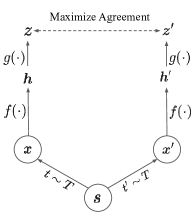
Self-supervised learning methods typically enforce semantic consistency across views to construct instance representations [27, 9]. This assumption is particularly true in the image domain because two views are typically generated from the same image. As shown in Fig. 1(a), the goal is to enforce the representations of these two views to be as close as possible in the feature space. In the video domain, these view-based contrastive approaches [45, 19] may be less effective as the visual appearance of an instance frequently and drastically changes across frames. For example, one person in a video can have different poses and perform different activities over time, indicating the states and semantics of an instance are likely to change across space and time. Enforcing spatio-temporal persistency throughout the video [19] would lead to representations only encoding minimally shared information across frames, which may negatively impact spatio-temporally fine-grained downstream tasks.

Furthermore, existing self-supervised methods typically focus on learning representations for holistic visual understanding tasks [9, 45], such as image classification and video action recognition. For dense prediction tasks, such as object detection, action localization and tracking, those models are enhanced by adding task specific heads. On the other hand, several approaches are designed to learn discriminative local features for dense prediction tasks [55, 63, 23, 62], but their performances on holistic visual understandings are often compromised [60]. In light of this, we are interested in learning representations that can be applied to both holistic and local video tasks.

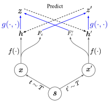
We propose Contextualized Spatio-Temporal Contrastive Learning (ConST-CL), illustrated in Fig. 1(b), to circumvent the undesirable strong spatio-temporal persistency enforced by the global contrastive objective. ConST-CL learns semantically consistent but discriminative local representations for various video downstream tasks, ranging from spatio-temporal action localization and object tracking to action recognition. Specifically, we design a projection function $g(\cdot,\cdot)$ to take not only the instance feature but also the context feature into account, where the instance feature is extracted from the source view of a video, and the context feature is sampled from the target view. This task enforces the model to be context-aware in a video and thus is a good proxy to learn discriminative local representations.

To address the imbalanced capability of learning holistic and local video representations, we design a simple two-branch module to facilitate the network to learn high-quality video representations both globally and locally in one unified self-supervised learning scheme.

We evaluate the learned representations on a variety of downstream tasks. For holistic representations, we evaluate with video action recognition on Kinetics400 [32], UCF101 [49] and HMDB51 [33] datasets. For local representations, we conduct experiments with spatio-temporal action localization on AVA-Kinetics [37] and AVA [25] datasets, and the single object tracking on the OTB2015 [58] dataset. Our experimental results show that by pretraining with ConST-CL, the learned representations adapt well across all studied datasets, surpassing recently proposed methods that use either supervised pretraining or the self-supervised pretraing [45, 62, 19, 22].

The main contributions of this work are:

• A region-based contrastive learning framework for fine-grained spatio-temporal representation learning.

• A contextualized region prediction task that facilitates learning semantically consistent while locally discrinimative video features.

• A simple network design to effectively reconcile simultaneous holistic and local representation learning.

• Competitive performance on 6 benchmarks, including spatio-temporal action localization, object tracking, and video action recognition.

Figure 2: Contextualized Spatio-Temporal Contrastive Learning. Two spatio-temporally distant views are randomly sampled from one video and their dense representation feature maps $\{F,F^{\prime}\}$ are extracted by the base network $f(x)$. Region features $\{h,h^{\prime}\}$ are pooled from respective dense feature maps by spatio-temporal ROIAlign and $F_{c}^{\prime}$ are a set of context features sampled from the dense feature maps $F^{\prime}$. The projection head $g(h,F_{c}^{\prime})$ is learned to transform representations $h$ from one view to the other, guided by the context features $F_{c}^{\prime}$. We use the transformer [52] architecture that takes region feature $h$ as Query and context features $F_{c}^{\prime}$ as Keys and Values. The InfoNCE loss is used to encourage the similarity between the reconstructed representations $z$ and their correspondences $h^{\prime}$.

2 Related Work

Self-supervised learning in images. To effectively learn representations from images, early self-supervised methods focus on designing pretext tasks by experts. Various pretext tasks have been proposed, including colorization [35], inpainting [42], denoising [53], egomotion prediction [2], context prediction [14], orientation prediction [21], spatial jigsaw puzzle [40], etc. Recent advances in image self-supervised learning stem mainly from minimizing contrastive loss [41] on instance discrimination tasks [16]. The contrastive objective effectively enforces representations of the same instance from different views to be similar, while it repels representations from different instances in the latent space. Representative frameworks in this category include NPID [59], MoCo [27, 10], SimCLR [9], etc.

Self-supervised learning in videos. In the video domain, self-supervised representation learning prospers in recent years. Contrastive objectives have been widely used to learn video representations for holistic recognition tasks [45, 19, 46, 64, 48]. Extensive pretext tasks have been exploited to learn good representation in videos. Compared with the image domain, videos naturally yield richer self-supervision signals. In [46], the goal is to enforce global context consistency and utilize long-short views of a video to align representations. In [56], the action and context features are factorized separately by learning from the conjugate examples in video dataset. Motion signals are also exploited for learning good representations [50, 26]. Temporal ordering of frames in a video has also been used for self-supervised representation learning. For instance, in [38, 36], temporal ordering of frames is enforced to learn representations by scuffling frames in a self-supervised manner. Similarly, forward and backward ordering of frames is used as the self-supervision signals for representation learning [57]. In addition, temporal cycle consistency is exploited to learn spatio-temporal correspondence between video frames [31, 54]. On the other hand, multi-modal signals, such as audio/visual and visual/text, have been used to learn representations in a self-supervised manner that outperform models based on a single modality [4, 5, 43, 39].

Local representations. Although existing methods focus on learning holistic representations on images or videos, several recent approaches explicitly model spatially fine-grained representations. In [8, 55], several constriave learning models have been developed for dense prediction tasks, such as object detection and image segmentation. In addition, augmented samples with pseudo ground-truth are generated to learn dense features for object detection [63, 13]. Other methods introduce location priors to group pixels for learning local features. For example, [66, 29, 51] use unsupervised masks and [44, 61] use pixel coordinates. In the video domain, many methods learn fine-grained features by leveraging inherent temporal augmentations to determine object correspondence [62, 65, 23, 31]. [23] randomly samples two images from a video to construct the contrastive pairs for self-supervised learning and shows improved performance on video tasks. [65] employs pretext tasks of determining whether frames are from the same video and their temporal ordering. [62] observes the emergence of correspondence by learning frame-level similarity. [31] enforces forward-backward temporal consistency to learn local correspondences in videos. Most of the existing approaches focus on learning local representations and do not emphasize performances on holistic tasks. [60] explicitly raises the question about simultaneously learning holistic and local representations but only focuses on the image domain.

Different from these related works, our method leverages video context during self-supervised learning by employing a novel region-based prediction tasks, and is designed to learn holistic and local representations simultaneously with self-supervision from unlabeled videos. Unlike most of the aforementioned methods that focus on learning either holistic or local representations, we emphasize the quality of both under one unified training scheme.

3 Method

In this section, we introduce the proposed self-supervised learning framework, Contextualized Spatio-Temporal Contrastive Learning (ConST-CL) for learning spatio-temporally fine-grained representations in videos.

3.1 Region-Based Contrastive Learning in Videos

Given a video, a simple contrastive learning algorithm randomly samples two video clips $\{x,x^{\prime}\}$, and applies random data augmentation on each video clip independently. Corresponding video-level representations $\{z,z^{\prime}\}\in\mathbb{R}^{C}$ are extracted by the network $f(\cdot)$ for computing a contrastive loss [41], with negative examples from other videos. We denote this video-level global contrastive loss as $\mathcal{L}_{g}$. This training objective enforces globally average-pooled features from the same video to be similar while it repels such features from different videos. However, no explicit supervision is enforced on local features, which play an important role for dense prediction tasks.

To enforce local supervision, one way is to extend [55] to the spatio-temporal domain. Given the dense feature maps $\{F,F^{\prime}\}\in\mathbb{R}^{T\times H\times W\times C}$ from $\{x,x^{\prime}\}$, where $T,W,H,C$ are time, height, width and channel dimention respectively, for each feature voxel $h_{i}\in F$, we find its correspondence $h_{j}^{\prime}\in F^{\prime}$ that it is closest to in the feature space to form a positive pair. Thus, the dense contrastive loss in a video can be formulated as:

$$z_{i} =g(h_{i})=\text{MLP}(h_{i}),$$ (1)

$$\mathcal{L}_{r} =\sum_{i}-\log\frac{\exp(z_{i}\cdot z_{j}^{\prime}/\tau)}{\exp(z_{i}\cdot z_{j}^{\prime}/\tau)+\sum_{k}{\exp(z_{i}\cdot\hat{z}_{k}/\tau)}},$$

s.t. $$\quad j=\operatorname*{argmin}_{j}h_{i}\cdot h^{\prime}_{j},$$ (2)

where MLP refers to a multi-layer perceptron, $\tau$ is the temperature parameter, $i$, $j$ and $k$ are grid indices, and $\{\hat{z}\}$ are representations from other videos. Here, we simply regard all the dense features from other videos as negative examples for loss computation.

Assuming that we have access to the location priors of regions of interest $\{r_{i}\}$, we can derive the vanilla region-based contrastive learning by organizing the representations using the region location:

$$z_{i} =g(h_{i})=\text{MLP}(\text{ROIAlign}(F,r_{i})),$$ (3)

where we override the notation $h_{i}$ to be the pooled region features, with $i$ being the region index. In this paper, we parameterize a region as a bounding box of a certain frame $r=\{t,x_{\textrm{min}},y_{\textrm{min}},x_{\textrm{max}},y_{\textrm{max}}\}$. The region representation $h_{i}$ is pooled from the dense feature map $F$ by ROIAlign [47].

The full learning objective is the linear combination of the global loss and the local loss weighted by the scale factor $\omega$. And we average over the $N$ mini-batch during training:

$$\mathcal{L}=\frac{1}{N}\sum\left(\mathcal{L}_{g}+\omega\mathcal{L}_{r}\right).$$ (4)

Figure 3: Balancing global and local losses. We analyze three different endpoints to impose global and local training losses. $\otimes$ indicates a pooling operation. Throughout the experiments, we find that by branching the res5 block in the network and applying $\mathcal{L}_{g}$ and $\mathcal{L}_{r}$ on R$5_{g}$ and R$5_{r}$ respectively, two losses mutually benefit and the representations thrive by co-training.

3.2 Contextualized Spatio-Temporal Contrastive Learning (ConST-CL)

The vanilla region-based contrastive learning framework described in Section 3.1 has one limitation: the loss always encourages the representations of the same instance at different timestamps to be similar, while the appearance of an instance in a video may change across frames. For example, one person in a video can appear in different poses and perform different activities. Simply enforcing the similarity of the same instance at different temporal locations of the video will inadvertently encourage the model to encode only the minimal information, which is less effective for downstream video understanding tasks.

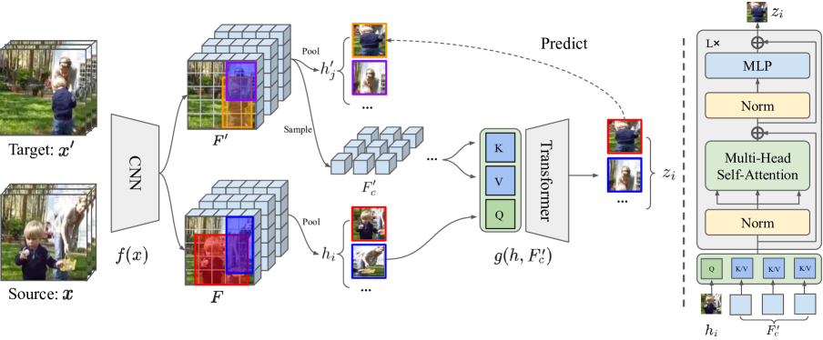
To resolve this issue, we propose a novel self-supervised method, Contextualized Spatio-Temporal Contrastive Learning (ConST-CL). In a nutshell, ConST-CL requires the network to learn to “reconstruct” the representation of a region in a target view given its representation from the source view and the context features around the target view.

$$z_{i} =g(h_{i},F_{c}^{\prime})=g(\text{ROIAlign}(F,r_{i}),F_{c}^{\prime}),$$ (5)

$$\mathcal{L}_{r} =\sum_{i}-\log\frac{\exp(z_{i}\cdot h_{j}^{\prime}/\tau)}{\exp(z_{i}\cdot h_{j}^{\prime}/\tau)+\sum_{k}{\exp(z_{i}\cdot\hat{h}_{k}/\tau)}},$$

s.t. $$\quad j=\operatorname*{argmin}_{j}h_{i}\cdot h^{\prime}_{j},$$ (6)

where $F^{\prime}_{c}$ denotes the set of context features around the target view, and $i$, $j$ and $k$ are region indices, and $\{\hat{h}\}$ are representations from other videos. Here we would like to note: (1) comparing with Eq. (3), we extend the representation decoding function $g(\cdot)$ from an unary function to a binary function $g(\cdot,\cdot)$ in Eq. (5); (2) we do not force bijective mapping between regions in two clips, so the different numbers of regions between views do not cause a problem. Eq.(5- 6) formulate ConST-CL in a general manner, which considers all regions from all frames. It might pose computation challenges, so in practice, we instead construct two sets of regions by sampling from one temporal slice of each feature map. The temporal sampling strategy will be discussed in the following ablation studies.

Fig. 2 shows an illustration of ConST-CL. Given a pooled region feature $h_{i}$ from the source view and a set of context features $F^{\prime}_{c}$ from the target view, a projection function $z_{i}=g(h_{i},F^{\prime}_{c})$ is learned with the objective to minimize the representation distance between the reconstructed relating representation $z_{i}$ and its corresponding native representation $h_{j}^{\prime}$ in the target view. The context features $F^{\prime}_{c}$ are a subset of feature voxels sampled from the dense feature map $F^{\prime}$. In our case, we subsample a few frames from the dense video representations $F^{\prime}$ along the temporal dimension. We define the number of frames used to construct $F^{\prime}_{c}$ as the context length, whose effect on the performance is studied in Section 4.4. Different from simply contrasting features that are projected into the shared feature space, ConST-CL requires every feature vector in $\{F,F^{\prime}\}$ to encode more information about itself and the context, such that with context features from another view, $g(\cdot,\cdot)$ can reconstruct the instance encoding conditionally.

We implement $g(\cdot,\cdot)$ using a transformer [52] architecture. First, we linearly project each instance feature vector from the source view $h_{i}$ to a Query token, and the context feature vectors from the target view $F_{c}^{\prime}$ to Key-Value token pairs. The multi-head cross-attention is then used to look up the Key-Value pairs by the Query token. Finally, we apply the InfoNCE loss [41] on the transformed instance feature $z_{i}$ and its correspondence $h_{j}^{\prime}$ using Eq. (6).

3.3 Region Generation

Random boxes. Generating random boxes on-the-fly during the training is the most straightforward method. For all of our related experiments, we randomly generate $8$ boxes on each frame. In Section 4.4, we show that our method performs interestingly well trained with these random boxes.

Boxes from low-level image cues. We also consider two methods to generate boxes from low-level image cues. Specifically, we use the SLIC [1] algorithm to generate $16$ superpixels on each frame. Following [29], we alternatively use the graph-based image segmentation method [20] to generate $16$ image segments for each frame.

Boxes from detectors. We also use off-the-shelf modern detectors to generate object-centric bounding boxes for weakly supervised learning. A CenterNet-based [68] person detector is employed to generate bounding boxes on persons only. As an alternative, we use a generic object detector, which is based on Cascade RCNN [17].

		Pre-training	AVA-Kinetics			AVA			Object Tracking
Method	Backbone	Dataset	mAP (GT)	mAP (Det)		mAP (GT)	mAP (Det)		Precision	Success
INet-sup [37]	I3D	K400	$35.9$	$22.9$		27.5	19.1		-	-
K400-sup	R3D50	K400	$26.7$	$19.8$		-	22.2		$71.2$	$51.46$
SimSiam [11]	R50	INet	-	-		-	-		$61.0$	$43.2$
VINCE [23]	R50	R2V2	-	-		-	-		$66.0$	$47.6$
SeCo [65]	R50	K400	-	-		-	-		$71.9$	$51.8$
VFS [62]	R50	K400	-	-		-	-		$73.9$	$52.5$
$\rho$MoCo [19]	Slow-only	K400	-	-		-	$20.3$		-	-
$\rho$BYOL [19]	Slow-only	K400	-	-		-	$23.4$		-	-
VFS-inflated	R3D50	K400	$34.6$	$25.9$		$29.1$	$22.4$		$73.3$	$52.7$
CVRL [45]	R3D50	K400	$31.6$	$24.1$		$24.9$	$18.4$		$75.4$	$53.7$
ConST-CL	R3D50	K400	$\mathbf{39.4}$	$\mathbf{30.5}$		$\mathbf{31.1}$	$\mathbf{24.1}$		$\mathbf{78.1}$	$\mathbf{55.2}$

Table 1: Downstream task performances based on pre-trained representations. The learned representations are evaluated for spatio-temporally fine-grained tasks, including spatio-temporal action recognition on the AVA v2.2 and AVA-Kinetics (using both ground-truth and detected person boxes) and single object tracking on OTB2015. ConST-CL achieves the state-of-the-art results across the board, suggesting the effectiveness of our proposed framework that is capable of coherently learning better local visual representations in videos.

3.4 Balancing Global and Local Losses

Existing methods [67, 62] have shown discriminative local features can be extracted by applying supervisory signals on holistic representations. Intuitively, adding constraints on both holistic and local representations are mutually beneficial, because discriminative local features would contribute to holistic recognition, while expressive holistic features could be derived from local features. In practice, however, we find that directly adding the proposed region-based local loss on the dense feature map right before the average pooling layer in the ResNet, the self-supervised training is less stable and sensitive to the hyper-parameters for balancing the global and local losses.

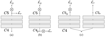
To address this issue, we propose a simple solution. As we use ResNet3D-50 as our base model, instead of adding the local loss on the $C5$ endpoint, we modify the ResNet architecture and replicate the $res5$ block, forming a “Y” structure, as shown in Fig. 3. Then the global and local losses are attached on endpoint $C5_{g}$ and $C5_{r}$, respectively, and they co-constrain the latent feature map in $C4$ during training. When fine-tuning the model for downstream tasks, we take either $C5_{g}$ or $C5_{r}$ branch depending on the task. This design introduces only moderate additional computes during the pre-training stage and is at no extra cost for fine-tuning and inference. We will show in Section 4.4 that the proposed “Y” structure results in better trade-off for both video-level and instance-level downstream tasks.

4 Experiments

We evaluate clip-level video representation models on the Kinetics400 [32] dataset following the linear probing protocol, and the UCF101 [49] and HMDB51 [33] datasets using both linear probing and fine-tuning. To evaluate the learned spatio-temporally fine-grained representations, we conduct experiments on the AVA-Kinetics [37] and AVA v2.2 [25] datasets for spatio-temporal action localization and the OTB2015 [58] dataset for single object tracking.

4.1 Implementation Details

We use the ResNet3D-50 (R3D50) as our backbone feature extractor following [45]. All features are $\ell_{2}$ normalized before being used to compute the self-supervised loss.

For the holistic representation learning branch, we use a 3-layer MLP with $2048$ hidden nodes to project a $2048$-dimensional feature vector into a $128$-dimensional feature vector. On the local representation learning branch, we use the same attention-based architecture as described in [52]. The attention units are stacked into multiple heads and layers to construct the ConST-CL head for the instance prediction task. In this work, the head of ConST-CL consists of 3-layer 3-head attention units with hidden dimension of $128$. We use the ReLU activation function without dropout. A final linear layer is used to project the $128$-dim feature vector back to $2048$-dim. We add spatio-temporal positional encodings to the query, key and value tokens before inputting into the transformer head in order to preserve location information. To construct contrastive pairs for local branch, we always sample examples from the center frame in both views for the experiments unless otherwise specified. The self-supervised pre-training is performed on the Kinetics400 [32] dataset. During evaluations, all the heads used for self-supervised learning are discarded.

All models are pre-trained with mini-batch of $1024$. During the pre-training, we use the SGD optimizer with momentum of $0.9$. The learning rate is linearly warmed-up to $40.96$ during the first $5$ epochs, followed by half-period cosine learning rate decay [28] to $0$. A weight decay of $10^{-6}$ is applied to all kernels. We set the temperature $\tau$ to be $0.1$ for the global loss and $0.2$ for the local loss. The scale factor $\omega$ is $0.01$ to balance the global and local losses.

For results in Table (1,2), we pre-train the backbone model for $200$k steps, which is around $850$ epochs on the Kinetics400 dataset with the randomly generated region boxes. And the context length is set to $5$. For all ablation studies, we use backbone models from a shorter pre-training schedule, which trains for $100$k steps.

4.2 Downstream Tasks

It is of great interest to understand whether one representation model can be applied to both holistic and local understandings, as intuitively the better local representations can facilitate holistic recognition tasks and vice versa. In this work, we apply the learned representation models to (1) video action recognition tasks that require holistic representations on the Kinetics400 [32], UCF101 [49] and HMDB51 [33] datastes; and (2) spatio-temporal action localization and single object tracking tasks that require local representations on the AVA-Kinetics [37], AVA v2.2 [25] and OTB2015 [58] datasets.

Video action recognition. we perform linear evaluation by fixing all the backbone weights on Kinetics400 [32], UCF101 [49] and HMDB51 [33]. The input is a $32$-frame video clip with temporal stride of $2$ and resolution of $224$. We train the linear classifier for $100$ epochs. We also use the pre-trained models to initialize the network and fine-tune all layers for $50$ epochs on UCF101 and HMDB51.

Spatio-temporal action localization. We attach the same action transformer head as in [22, 37] to our R3D50 backbone, and follow the setting in [37] for simplicity. We train our model with ground-truth person bounding boxes and use either ground-truth boxes or boxes generated using off-the-shelf person detectors for region proposals during evaluation. The model is trained with batch size $256$ for $50$k steps. The input has $32$ frames with resolution of $400$ and temporal stride of $2$.

Single object tracking. We also evaluate our learned representations via single object tracking task, which requires semantically consistent spatio-temporal features to determine object-level correspondence. We follow the same practice as in [62, 23, 65] to adopt the SiameseFC [6] as the tracker and modify the spatial stride and dilation rate in the $res_{4}$ and $res_{5}$ blocks. Note that our backbone is a 3D-convolutional network, and for each input frame we also sample its neighboring $n$ frames from each side and use the $2n+1$ frames as the input. After the $res_{5}$ block, we slice the center frame along the time dimension of the local feature map $F$ for the input to the tracking head. Here we use $n=2$ as the largest temporal kernel in the network is $5$. We use the pre-trained checkpoint to initialize the backbone and fine-tune the tracker for all experiments.

4.3 Main Results

In Table 1, we study the model performance on dense vision tasks by using the pre-trained models from different methods. We evaluate the spatio-temporal action localization on the AVA-Kinetics [37] and AVA v2.2 [25]. Following [37, 22], the models are evaluated under two settings: using either ground-truth boxes or detected boxes as region proposals on the validation set. On AVA-Kinetics, ConST-CL achieves $39.4\%$ mAP when using ground-truth boxes and $30.5\%$ mAP when using detected boxes, outperforming the supervised method [37] by a large margin. ConST-CL also outperforms the baseline self-supervised method CVRL [45] model with more than $24\%$ relative performance gain. In addition, we compare to the VFS [62] which is designed for dense vision tasks. As VFS uses 2D ResNet, we follow the common practice to inflate all 2D kernels in the network into 3D [7] and load the pre-trained weights from VFS for the fair comparison. In the table, ConST-CL outperforms the VFS-inflated method by more than $4.6\%$ mAP, showing the effectiveness of our proposed method on spatio-temporal action recognition task. On the AVA v2.2, we observe similar trend that ConST-CL outperforms competing methods, achieving $31.1\%$ and $24.1\%$ mAP using ground-truth and detected boxes respectively.

On OTB2015 [58], we first compare with prior methods designed for dense task only. Table 1 shows that ConST-CL outperforms the evaluated methods by a large margin. Specifically, compared to VFS [62], ConST-CL achieves $78.1\%$($+\Delta 4.2\%$) in precision score and $55.2\%$($+\Delta 2.7\%$) in success score. To rule out the effect of architecture difference (2D network vs. 3D network), we inflate the 2D ResNet into 3D and load the VFS pre-trained checkpoint, denoted as VFS-inflated in the table. Compared to VFS, VFS-inflated performs similarly to its 2D counterpart, which indicates the effect of this architecture difference on the tracking task is insignificant. When compared with CVRL, ConST-CL achieves clear performance gain for single object tracking on the OTB2015 benchmark.

In Table 2, our method performs comparable to CVRL and $\rho$MOCO ($\rho$=2) using linear probing and achieves competitive fine-tuning results with top-1 accuracy of $94.8\%$ and $71.9\%$ on UCF101 and HMDB51, respectively. It is worth pointing out that our method improves upon CVRL on fine-tuning UCF101 and HMDB51, even though we do not use any extra supervision on holistic representations other than the CVRL’s loss $\mathcal{L}_{g}$. These findings are consistent with our intuition that the holistic and the local representation modeling can be mutually beneficial. In our method, the two losses simultaneously contribute to and constrain on the latent feature map $C4$ in the network. These results also demonstrate the effectiveness of the proposed model design that coherently organizes different levels of representations in a single framework.

Finally, in Table 3 we report the model size and computational cost including both the backbone and the SSL heads in different video self-supervised learning methods. Comparing to CVRL, ConST-CL increased model sizes and computational cost moderately, mainly due to the branched $res_{5}$ block and additional transformer head. The Slow-only network and training strategy used in [19] is different from ours, making the side-to-side comparison difficult. Thus we leave the results in the table for reference.

	Linear				Fine-tune
Method	K400	UCF	HMDB		UCF	HMDB
VINCE [23]	$49.1$	-	-		-	-
SeCo [65]	$61.9$	-	-		$88.3$	$55.6$
VFS-inflated [62]	$33.1$	-	-		$71.4$	$41.0$
$\rho$MoCo ($\rho$=$2$) [19]	$67.4$	-	-		$93.2$	-
$\rho$BYOL ($\rho$=$4$) [19]	$\mathbf{71.5}$	-	-		$\mathbf{95.5}$	$\mathbf{73.6}$
CVRL [45]	$66.1$	$\mathbf{89.2}$	$57.3$		$92.2$	$66.7$
ConST-CL	$66.6$	$89.1$	$\mathbf{59.9}$		$94.8$	$71.9$

Table 2: Downstream video action recognition. ConST-CL achieves competitive results on fine-tuning experiments, indicating it can learn strong holistic visual representations in videos.

Method	Frames	Params (M)	FLOPs (G)
CVRL [45]	16$\times$2	$44.6$	$91.2$
$\rho$MOCO ($\rho$=$2$) [19]	8$\times$2	$44.6$	$83.6$
$\rho$MOCO ($\rho$=$2$) [19]	16$\times$2	$44.6$	$167.0$
$\rho$BYOL ($\rho$=$4$) [19]	16$\times$4	$44.6$	$334.0$
ConST-CL	16$\times$2	$71.7$	$113.0$

Table 3: Model sizes and computational costs for different SSL methods with video-based networks. The SSL heads are included for the parameter and FLOPS counts.

Method	Sampling	UCF	HMDB	AVA-K	OTB
CVRL	-	$91.6$	$66.2$	$30.9$	$75.9$
ConST-CL	Random	$56.2$	$57.8$	$34.8$	$75.4$
ConST-CL	Center	$94.1$	$67.7$	$36.9$	$77.1$
ConST-CL	Nearest	$93.8$	$68.1$	$36.9$	$76.4$

Table 4: Ablation on the temporal sampling strategy. The “Center” and “Nearest” temporal sampling strategy perform equally well and better than “Random” sampling for ConST-CL.

Method	Endpoint	UCF	HMDB	AVA-K	OTB
CVRL	-	$91.6$	$66.2$	$30.9$	$75.9$
ConST-CL	$C4_{p}$	$93.5$	$67.5$	$32.0$	$75.3$
ConST-CL	$C5$	$93.4$	$66.7$	$33.6$	$74.3$
ConST-CL	$C5_{g}$+$C5_{r}$	$94.3$	$68.7$	$36.7$	$77.7$

Table 5: Ablation on the loss endpoints. We apply region-based contrastive loss on different endpoints and show that the $C5_{g}$+$C5_{r}$ configuration achieves the best trade-off between the global and local losses with the best downstream task performances.

Context	Loss	UCF	HMDB	AVA-Kinetics			OTB
length	endpoint(s)	Top-1	Top-1	mAP (GT)	mAP (Det)		Precision	Success	$\#$Params (M)	$\#$FLOPs (G)
-	R5	$91.6$	$66.2$	$30.9$	$23.4$		$75.9$	$53.6$	$44.6$	$45.6$
$0$	2R5	$91.8$	$66.0$	$35.3$	$27.5$		$75.4$	$56.6$	$77.7$	$55.5$
$1$	2R5	$93.4$	$66.7$	$36.7$	$28.0$		$77.7$	$55.0$	$71.7$	$55.6$
$3$	2R5	$93.7$	$67.4$	$36.9$	$28.1$		$77.5$	$54.5$	$71.7$	$56.1$
$5$	2R5	$93.4$	$67.5$	$37.6$	$28.1$		$79.0$	$55.4$	$71.7$	$56.5$

Table 6: Ablation study on the context length and the computational overhead. “-” indicates no ConST-CL is used and the model is only trained with the $\mathcal{L}_{g}$; “0” indicates no context is provided and the model simply degrades to the vanilla region-based contrastive learning. From the table, we observe the trend that more context is helpful to learn better spatio-temporal representations. We notice the number of parameter increment is largely from the duplicated $res5$ block while our transformer based head is more parameter efficient than the MLP head for the region-based contrastive learning.

	UCF	AVA-K	OTB
Box type	Top-1	mAP (GT)	Precision	Success
Random	$94.3$	$36.9$	$77.0$	$54.0$
SLIC [1]	$93.4$	$36.4$	$76.3$	$53.7$
FH [20]	$94.1$	$36.9$	$77.1$	$54.3$
Person Detector	$93.4$	$36.7$	$77.7$	$55.0$
Object Detector	$93.7$	$37.2$	$77.8$	$54.1$

Table 7: Ablation study on the box type. When applying different types of boxes during the self-supervised training, we find that model learns equally well regardless of the region location quality.

4.4 Ablation Study

Temporal sampling strategy. To construct the contrastive region pairs, we sample one frame from the source and the target clip respectively. In Table 4, we study three different temporal sampling strategies. For “random” strategy, we randomly sample frames from the source and the target views to construct the contrastive pairs. For “center” strategy, we simply choose the center frame from the dense feature maps in both views for ConST-CL. For “nearest” strategy, we always choose the temporally closest frame pairs from two views. If two randomly sampled clips temporally overlap, then we draw samples from their overlapping frames. Otherwise, frames at the closest two ends of the two video clips are selected. Table 4 shows that the “random” sampling strategy is consistently worse than the other approaches. This can be attributed to that the temporally random sampling introduces significant noise and negatively affect the model performance. We do not see significant performance differences by using the “center” or “nearest” sampling strategy. For the simplicity, we choose the “center” sampling strategy throughout our experiments.

Loss endpoints. We analyze how global and local contrastive losses can be integrated together for vision tasks. In this study, we attach the proposed local loss to different endpoints of the network and analyze how it interacts with the global loss. As shown in Fig. 3(a) the region features are from the C5 endpoint for this model. For the model in Fig. 3(b), we first perform a 2$\times$2 average pooling on the C4 feature map to reduce its spatial resolution from 14$\times$14 to 7$\times$7 and then apply the region-level loss. For the model in Fig 3(c), we duplicates the $res5$ block of the network and then apply the global loss on $\text{C5}_{g}$ branch and the region loss on the $\text{C5}_{r}$ branch respectively. During the inference stage for the model in Fig 3(c), we use feature maps from $\text{C5}_{g}$ and $\text{C5}_{r}$ for video and instance-level tasks respectively. In Table 5, we observe that by simply adding the proposed region-based contrastive loss on C4_p or C5, ConST-CL outperforms the baseline method CVRL on downstream tasks already. By branching the $res5$ block as shown in Fig 3(c), we achieve the best trade-off of two losses and the holistic and local representations obtain better performance gains on downstream tasks.

Context length. We study the effect of contextualization by varying the number of feature maps sampled along the time axis from the target view to input to the ConST-CL transformer head. Different number of context length indicates the number of feature maps sampled along the time axis. Note that when the context length is zero, the method simply degrades to the vanilla region-based contrastive learning described in Section 3.1. Table 6 shows our model learns better representations as the context length is increased. This can be attributed to that as more context features provide richer information about the target view, the model can learn a better decoder function $g(\cdot,\cdot)$, resulting in higher-quality spatio-temporal representations. In Table 6, we also present the number of model parameters and FLOPs for one pass of self-supervised training. Comparing the vanilla region-based model (second row) to the baseline model CVRL (first row), we note that the number of model parameters is increased by $74.2\%$ and the number of FLOPs is increased by $20.9\%$, where the overheads largely result from the duplicated $res5$ block. When switching to the proposed transformer decoder with context length equals to $1$, the number of model parameters is decreased to $71.76$M while the FLOPs is increased by $0.16$B. This is due to the fact that we use multi-head self-attention with fewer hidden units, which is more parameter efficient. Finally, when increasing context lengths, we notice only slight increases in the number of FLOPs.

Boxes type. Table 7 shows how different location priors affect the representations learning. We study three types of boxes generated using different methods: randomly generated boxes, boxes derived from low-level image cues and detector-generated boxes. Overall, our method performs equally well regardless whether region locations are accurate or not. We reason that each region could be understood as an instance crop in the scene and ConST-CL does not require the crop to be object-centric. This observation is aligned with previous self-supervised learning methods on images [27, 9] and videos [45]. The experiment suggests the robustness of the proposed method.

4.5 Limitations

One missing piece in the current framework is the self-supervisory signal for learning even finer-grained representations. We hope to enrich our method by incorporating dense self-supervision in the future. Moreover, the current solution of organizing global-local self-supervisory signals is limited to the convolutional neural network backbone. For the recent vision transformer (ViT) [15], it is non-trivial to apply our proposed method directly in its current form.

5 Conclusion

In this paper, we propose a novel self-supervised learning framework that facilitates learning versatile spatio-temporally fine-grained representations in videos. A simple architecture design is proposed to reconcile holistic and local representations learning in one single framework. Extensive experiments are carried out to demonstrate the efficacy of the proposed method. In the future, we plan to experiment on more video tasks, such as video segmentation and temporal localization.

Acknowledgment. We thank Olivier Henaff (DeepMind) for providng image segmentation code; Ang Li (DeepMind) for the help with AVA-Kinetics; Xiao Zhang (U. Chicago) and Jianing Wei (Google) for the help with object tracking.

Appendix A Model Architectures

We illustrate the model architectures that are used in the ConST-CL framework.

A.1 Base network $\boldsymbol{f(\cdot)}$

Table 8 describes the base model architecture that is proposed for reconciling global and local training signals.

Stage	Network	Input from	Output size $T\times S^{2}$
raw clip	-	-	$32\times 224^{\text{2}}$
data	stride 2, 1${}^{\text{2}}$	raw clip	$16\times 224^{\text{2}}$
res1	$\textbf{5}\times 7^{\text{2}}$, 64	data	$8\times 112^{\text{2}}$
	stride 2, 2${}^{\text{2}}$
pool1	$1\times 3^{\text{2}}$ max	res1	$8\times 56^{\text{2}}$
	stride 1, 2${}^{\text{2}}$
res2	$\left[\begin{array}[]{c}\text{1$\times$1${}^{\text{2}}$, {64}}\\[-0.80005pt] \text{1$\times$3${}^{\text{2}}$, {64}}\\[-0.80005pt] \text{1$\times$1${}^{\text{2}}$, {256}}\end{array}\right]$$\times$3	pool1	$8\times 56^{\text{2}}$
res3	$\left[\begin{array}[]{c}\text{1$\times$1${}^{\text{2}}$, {128}}\\[-0.80005pt] \text{1$\times$3${}^{\text{2}}$, {128}}\\[-0.80005pt] \text{1$\times$1${}^{\text{2}}$, {512}}\end{array}\right]$$\times$4	res2	$8\times 28^{\text{2}}$
res4	$\left[\begin{array}[]{c}\text{\text@underline{3$\times$1${}^{\text{2}}$}, {256}}\\[-0.80005pt] \text{1$\times$3${}^{\text{2}}$, {256}}\\[-0.80005pt] \text{1$\times$1${}^{\text{2}}$, {1024}}\end{array}\right]$$\times$6	res3	$8\times 14^{\text{2}}$
res5r	$\left[\begin{array}[]{c}\text{\text@underline{3$\times$1${}^{\text{2}}$}, {512}}\\[-0.80005pt] \text{1$\times$3${}^{\text{2}}$, {512}}\\[-0.80005pt] \text{1$\times$1${}^{\text{2}}$, {2048}}\end{array}\right]$$\times$3	res4	$8\times 7^{\text{2}}$
res5g	$\left[\begin{array}[]{c}\text{\text@underline{3$\times$1${}^{\text{2}}$}, {512}}\\[-0.80005pt] \text{1$\times$3${}^{\text{2}}$, {512}}\\[-0.80005pt] \text{1$\times$1${}^{\text{2}}$, {2048}}\end{array}\right]$$\times$3	res4	$8\times 7^{\text{2}}$

Table 8: Base network $\boldsymbol{f(\cdot)}$: a ResNet3D-50 (R3D-50) based encoder.

A.2 ConST-CL head $\boldsymbol{g(\cdot,\cdot)}$

Table 9 describes the projection head we use for achieving the instance prediction task.

Stage	Input, Dimension	Network	Output
Linear project	$\boldsymbol{h}$, N$\times$2048	n_nodes=128	Query
Linear project	$\boldsymbol{F_{c}^{\prime}}$, M$\times$2048	n_nodes=128	Key
Linear project	$\boldsymbol{F_{c}^{\prime}}$, M$\times$2048	n_nodes=128	Value
MHSA	Query, N$\times$128	hidden_size=128	Hidden
	Key, M$\times$128	n_heads=3
	Value, M$\times$128	n_layers=3
Linear project	Hidden, N$\times$128	n_nodes=2048	$\boldsymbol{z}$

Table 9: ConST-CL head $\boldsymbol{g(\cdot,\cdot)}$: a transformer-based decoder. The inputs are the region features $\boldsymbol{h}$ and the context features $\boldsymbol{F_{c}^{\prime}}$ and the outputs are the transformed features $\boldsymbol{z}$. N and M are the number of tokens of $\boldsymbol{h}$ and $\boldsymbol{F_{c}^{\prime}}$ respectively.

Appendix B Region Generation

In this section, we detail three options to generate region priors that we study for training ConST-CL.

Random boxes. For all of our related experiments, we randomly generate $8$ boxes on each frame. The boxes are constrained to have aspect ratio within $[0.5,2]$ and size within $[0.1,0.5]$ of the image size.

Boxes from low-level image cues. We use the SLIC [1] algorithm to generate $16$ superpixels on each frame. Following [29], we alternatively use the graph-based image segmentation method [20] to generate $16$ image segments for each frame. We use two scales to generate segments, the scale $s$ and minimum cluster size $c$, and $s=c\in\{500,1000\}$ in practice. After the segments generation, we convert each segment into its minimal bounding box and only keep those with width/height between $[0.05,0.7]$ of the image width/height.

Boxes from detectors. We also use off-the-shelf modern detectors to generate object-centric bounding boxes for weakly supervised learning. A CenterNet-based [68] person detector is employed to generate bounding boxes on persons only. As an alternative, we use a generic object detector, which is based on Cascade RCNN [17].

Appendix C Downstream tasks

C.1 Action Recognition

On all video action recognition datasets, we use the video clip of $32$ frames with temporal stride $2$ as input. During training, the temporally consistent random data augmentation [45] of cropping, resizing and flipping are applied and the resolution is set to $224\times 224$. During evaluation, we densely sample $10$ clips with resolution $256\times 256$ from each video and apply a 3-crop evaluation following [18].

Linear Evaluation. On action recognition datasets, we train a linear classifier with fixed backbone weights using the SGD optimizer with momentum of $0.9$. On Kineitcs400 [32], the linear classifier is trained for $100$ epochs with learning rate of $32$ and batch size of $1024$. On UCF101 [49] and HMDB51 [33], the linear classifier is trained for $50$ epochs with learning rate of $0.84$ and batch size of $128$. No dropout and weight decay are applied.

Fine-tuning. On UCF101 [49] and HMDB51 [33], we use the pre-trained models to initialize the network and fine-tune all layers for $50$ epochs. We use batch size of $128$, weight decay of $1\text{e-}5$ and dropout rate of $0.5$ during fine-tuning. The learning rate is set to $0.72$ and $0.84$ for UCF101 and HMDB51 respectively.

C.2 Spatio-temporal Action Localization

We use the same action transformer head as in [22, 37] to our R3D-50 backbone and follow the setting in [37]. The model is fine-tuned with batch size $256$ for $50$k steps, which is around $36$ epochs on AVA-Kinetics [37]. The input has $32$ frames with resolution $400$ and temporal stride $2$. We use the SGD optimizer with momentum $0.9$ during the fine-tuning. On AVA-Kinetics, the learning rate is $1\text{e-}2$ and the weight decay is $1\text{e-}7$. On AVA [25], the learning rate is set to $3\text{e-}2$ and the weight decay is $1\text{e-}4$. During evaluation, we use the same set of detected boxes in [37] for AVA-Kinetics and in [19] for AVA v2.2 for a fair comparison.

C.3 Object Tracking

To evaluate on OTB2015 [58] dataset, we follow the same practice as in [62, 23, 65] to adopt the SiameseFC [6] as the tracker. Specifically, we modify the spatial stride and dilation rate to be $(1,2)$ and $(1,4)$ in the first layer of the $res_{4}$ and $res_{5}$ blocks. These modifications allows us to increase the feature map resolution without impacting on the pre-trained model. We fine-tune the tracker on GOT-10K [30] dataset using the SGD optimizer with momentum of $0.9$. We use batch size of $256$, learning rate of $0.1$ and weight decay of $1\text{e-}4$ and the tracker is fine-tuned for 20 epochs.

Appendix D Visualization

D.1 Attention

Source	Thumbnail	Target	Attention

Figure 4: Visualization of the attention during the training. We use boxes from the object detector to pool region features from the source view as the query in order to generate the attention maps given the context (features from the target view). Interestingly, the model learns to attend to not only the corresponding instance in the target frame, but also to some other semantically meaningful objects the instance potentially interacts with.

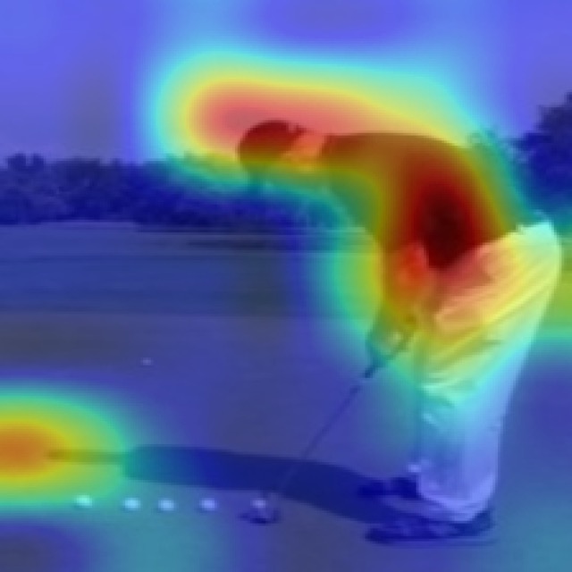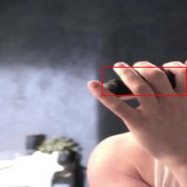
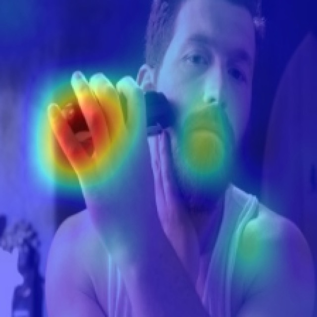
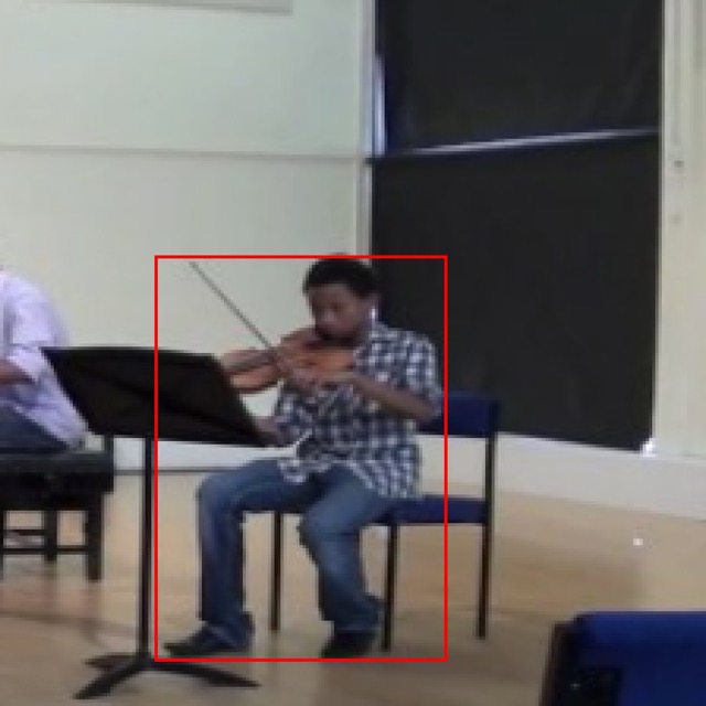
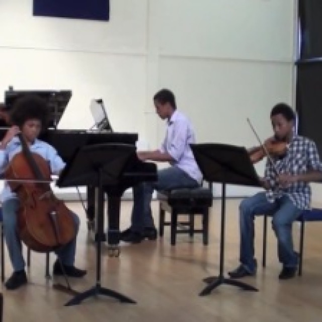
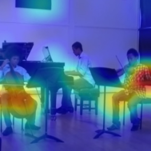
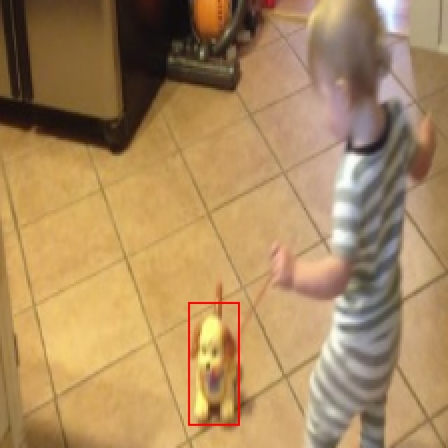
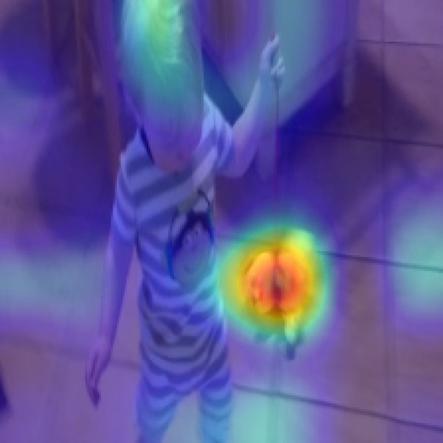
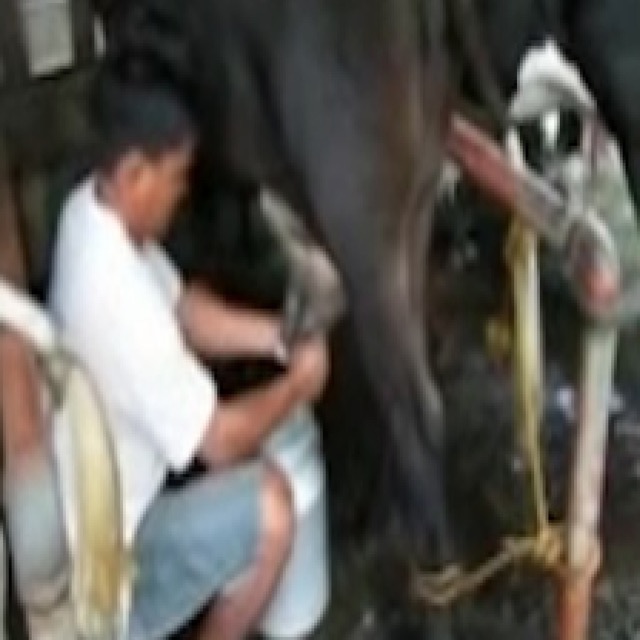
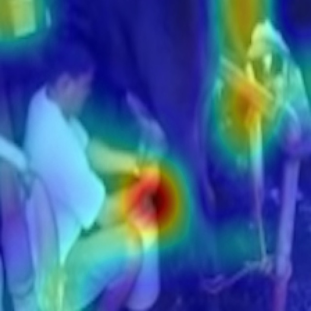
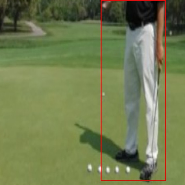
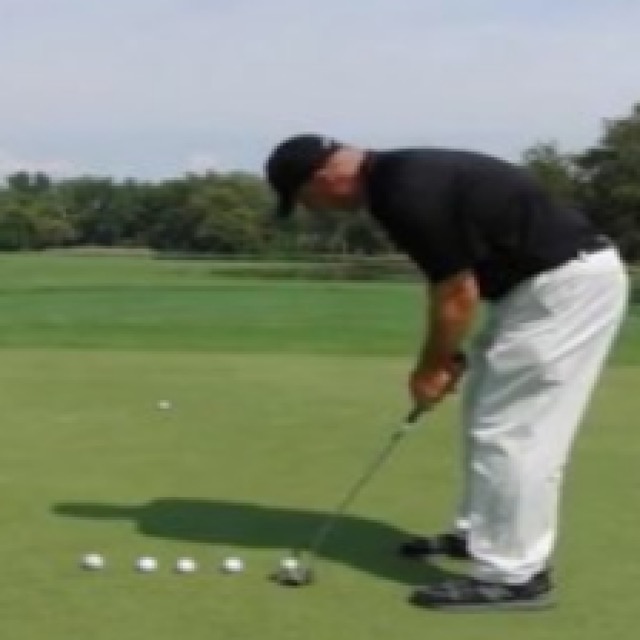
We visualize the learned attention map during the training in Figure 4. For visualization purpose only, we use the boxes from the object detector to pool the region features in the source views to generate the attention maps. The model is trained with the randomly generated boxes as described in the paper. In Figure 4, we visualize the center frames in the source and the target views and the source frames are superimposed with one box for visualization. The zoomed-in thumbnails are presented in the second column. Given the context (features from the target views), we use these thumbnails’ region feature as the query to generate the attention maps shown in the fourth column. It is interesting to observe that the model learns to attend to not only the corresponding instance in the target view, but also to some other semantically meaningful objects the instance potentially interacts with.

D.2 Visual Object Tracking

Input	Prediction

Figure 5: Qualitative results for visual object tracking on OTB2015 [58]. Best view in color.

We provide some qualitative results on visual object tracking on OTB2015 [58] in Figure 5. The results show that our tracker could robustly track objects under different scenarios.

References

- [1] Radhakrishna Achanta, Appu Shaji, Kevin Smith, Aurelien Lucchi, Pascal Fua, and Sabine Süsstrunk. Slic superpixels compared to state-of-the-art superpixel methods. TPAMI, 2012.
- [2] Pulkit Agrawal, Joao Carreira, and Jitendra Malik. Learning to see by moving. In ICCV, 2015.
- [3] Hassan Akbari, Linagzhe Yuan, Rui Qian, Wei-Hong Chuang, Shih-Fu Chang, Yin Cui, and Boqing Gong. Vatt: Transformers for multimodal self-supervised learning from raw video, audio and text. In NeurIPS, 2021.
- [4] Jean-Baptiste Alayrac, Adria Recasens, Rosalia Schneider, Relja Arandjelovic, Jason Ramapuram, Jeffrey De Fauw, Lucas Smaira, Sander Dieleman, and Andrew Zisserman. Self-supervised multimodal versatile networks. In NeurIPS, 2020.
- [5] Humam Alwassel, Dhruv Mahajan, Bruno Korbar, Lorenzo Torresani, Bernard Ghanem, and Du Tran. Self-supervised learning by cross-modal audio-video clustering. arXiv preprint arXiv:1911.12667, 2019.
- [6] Luca Bertinetto, Jack Valmadre, Joao F Henriques, Andrea Vedaldi, and Philip HS Torr. Fully-convolutional siamese networks for object tracking. In ECCV, 2016.
- [7] Joao Carreira and Andrew Zisserman. Quo vadis, action recognition? a new model and the kinetics dataset. In CVPR, 2017.
- [8] Krishna Chaitanya, Ertunc Erdil, Neerav Karani, and Ender Konukoglu. Contrastive learning of global and local features for medical image segmentation with limited annotations. arXiv preprint arXiv:2006.10511, 2020.
- [9] Ting Chen, Simon Kornblith, Mohammad Norouzi, and Geoffrey Hinton. A simple framework for contrastive learning of visual representations. In ICML, 2020.
- [10] Xinlei Chen, Haoqi Fan, Ross Girshick, and Kaiming He. Improved baselines with momentum contrastive learning. arXiv preprint arXiv:2003.04297, 2020.
- [11] Xinlei Chen and Kaiming He. Exploring simple siamese representation learning. In CVPR, 2021.
- [12] Jacob Devlin, Ming-Wei Chang, Kenton Lee, and Kristina Toutanova. Bert: Pre-training of deep bidirectional transformers for language understanding. arXiv preprint arXiv:1810.04805, 2018.
- [13] Jian Ding, Enze Xie, Hang Xu, Chenhan Jiang, Zhenguo Li, Ping Luo, and Gui-Song Xia. Unsupervised pretraining for object detection by patch reidentification. arXiv preprint arXiv:2103.04814, 2021.
- [14] Carl Doersch, Abhinav Gupta, and Alexei A Efros. Unsupervised visual representation learning by context prediction. In ICCV, 2015.
- [15] Alexey Dosovitskiy, Lucas Beyer, Alexander Kolesnikov, Dirk Weissenborn, Xiaohua Zhai, Thomas Unterthiner, Mostafa Dehghani, Matthias Minderer, Georg Heigold, Sylvain Gelly, et al. An image is worth 16x16 words: Transformers for image recognition at scale. In ICLR, 2021.
- [16] Alexey Dosovitskiy, Jost Tobias Springenberg, Martin Riedmiller, and Thomas Brox. Discriminative unsupervised feature learning with convolutional neural networks. In NeurIPS, 2014.
- [17] Xianzhi Du, Barret Zoph, Wei-Chih Hung, and Tsung-Yi Lin. Simple training strategies and model scaling for object detection. arXiv preprint arXiv:2107.00057, 2021.
- [18] Christoph Feichtenhofer, Haoqi Fan, Jitendra Malik, and Kaiming He. Slowfast networks for video recognition. In ICCV, 2019.
- [19] Christoph Feichtenhofer, Haoqi Fan, Bo Xiong, Ross Girshick, and Kaiming He. A large-scale study on unsupervised spatiotemporal representation learning. In CVPR, 2021.
- [20] Pedro F Felzenszwalb and Daniel P Huttenlocher. Efficient graph-based image segmentation. IJCV, 2004.
- [21] Spyros Gidaris, Praveer Singh, and Nikos Komodakis. Unsupervised representation learning by predicting image rotations. In ICLR, 2018.
- [22] Rohit Girdhar, Joao Carreira, Carl Doersch, and Andrew Zisserman. Video action transformer network. In CVPR, 2019.
- [23] Daniel Gordon, Kiana Ehsani, Dieter Fox, and Ali Farhadi. Watching the world go by: Representation learning from unlabeled videos. arXiv preprint arXiv:2003.07990, 2020.
- [24] Jean-Bastien Grill, Florian Strub, Florent Altché, Corentin Tallec, Pierre H Richemond, Elena Buchatskaya, Carl Doersch, Bernardo Avila Pires, Zhaohan Daniel Guo, Mohammad Gheshlaghi Azar, et al. Bootstrap your own latent: A new approach to self-supervised learning. arXiv preprint arXiv:2006.07733, 2020.
- [25] Chunhui Gu, Chen Sun, David A Ross, Carl Vondrick, Caroline Pantofaru, Yeqing Li, Sudheendra Vijayanarasimhan, George Toderici, Susanna Ricco, Rahul Sukthankar, et al. Ava: A video dataset of spatio-temporally localized atomic visual actions. In CVPR, 2018.
- [26] Tengda Han, Weidi Xie, and Andrew Zisserman. Self-supervised co-training for video representation learning. In NeurIPS, 2020.
- [27] Kaiming He, Haoqi Fan, Yuxin Wu, Saining Xie, and Ross B Girshick. Momentum contrast for unsupervised visual representation learning. In CVPR, 2019.
- [28] Tong He, Zhi Zhang, Hang Zhang, Zhongyue Zhang, Junyuan Xie, and Mu Li. Bag of tricks for image classification with convolutional neural networks. In CVPR, 2019.
- [29] Olivier J Hénaff, Skanda Koppula, Jean-Baptiste Alayrac, Aaron van den Oord, Oriol Vinyals, and João Carreira. Efficient visual pretraining with contrastive detection. In ICCV, 2021.
- [30] Lianghua Huang, Xin Zhao, and Kaiqi Huang. Got-10k: A large high-diversity benchmark for generic object tracking in the wild. TPAMI, 2021.
- [31] Allan Jabri, Andrew Owens, and Alexei A Efros. Space-time correspondence as a contrastive random walk. In NeurIPS, 2020.
- [32] Will Kay, Joao Carreira, Karen Simonyan, Brian Zhang, Chloe Hillier, Sudheendra Vijayanarasimhan, Fabio Viola, Tim Green, Trevor Back, Paul Natsev, et al. The kinetics human action video dataset. arXiv preprint arXiv:1705.06950, 2017.
- [33] Hildegard Kuehne, Hueihan Jhuang, Estíbaliz Garrote, Tomaso Poggio, and Thomas Serre. Hmdb: a large video database for human motion recognition. In ICCV, 2011.
- [34] Zhenzhong Lan, Mingda Chen, Sebastian Goodman, Kevin Gimpel, Piyush Sharma, and Radu Soricut. Albert: A lite bert for self-supervised learning of language representations. 2020.
- [35] Gustav Larsson, Michael Maire, and Gregory Shakhnarovich. Colorization as a proxy task for visual understanding. In CVPR, 2017.
- [36] Hsin-Ying Lee, Jia-Bin Huang, Maneesh Singh, and Ming-Hsuan Yang. Unsupervised representation learning by sorting sequences. In ICCV, 2017.
- [37] Ang Li, Meghana Thotakuri, David A Ross, João Carreira, Alexander Vostrikov, and Andrew Zisserman. The ava-kinetics localized human actions video dataset. arXiv preprint arXiv:2005.00214, 2020.
- [38] Ishan Misra, C Lawrence Zitnick, and Martial Hebert. Shuffle and learn: unsupervised learning using temporal order verification. In ECCV, 2016.
- [39] Pedro Morgado, Nuno Vasconcelos, and Ishan Misra. Audio-visual instance discrimination with cross-modal agreement. arXiv preprint arXiv:2004.12943, 2020.
- [40] Mehdi Noroozi and Paolo Favaro. Unsupervised learning of visual representations by solving jigsaw puzzles. In ECCV, 2016.
- [41] Aaron van den Oord, Yazhe Li, and Oriol Vinyals. Representation learning with contrastive predictive coding. arXiv preprint arXiv:1807.03748, 2018.
- [42] Deepak Pathak, Philipp Krahenbuhl, Jeff Donahue, Trevor Darrell, and Alexei A Efros. Context encoders: Feature learning by inpainting. In CVPR, 2016.
- [43] Mandela Patrick, Yuki M Asano, Polina Kuznetsova, Ruth Fong, João F Henriques, Geoffrey Zweig, and Andrea Vedaldi. On compositions of transformations in contrastive self-supervised learning. In ICCV, 2021.
- [44] Pedro O Pinheiro, Amjad Almahairi, Ryan Y Benmalek, Florian Golemo, and Aaron Courville. Unsupervised learning of dense visual representations. arXiv preprint arXiv:2011.05499, 2020.
- [45] Rui Qian, Tianjian Meng, Boqing Gong, Ming-Hsuan Yang, Huisheng Wang, Serge Belongie, and Yin Cui. Spatiotemporal contrastive video representation learning. In CVPR, 2021.
- [46] Adrià Recasens, Pauline Luc, Jean-Baptiste Alayrac, Luyu Wang, Florian Strub, Corentin Tallec, Mateusz Malinowski, Viorica Patraucean, Florent Altché, Michal Valko, et al. Broaden your views for self-supervised video learning. In ICCV, 2021.
- [47] Shaoqing Ren, Kaiming He, Ross Girshick, and Jian Sun. Faster r-cnn: Towards real-time object detection with region proposal networks. In NeurIPS, 2015.
- [48] Ankit Singh, Omprakash Chakraborty, Ashutosh Varshney, Rameswar Panda, Rogerio Feris, Kate Saenko, and Abir Das. Semi-supervised action recognition with temporal contrastive learning. In CVPR, 2021.
- [49] Khurram Soomro, Amir Roshan Zamir, and Mubarak Shah. Ucf101: A dataset of 101 human actions classes from videos in the wild. arXiv preprint arXiv:1212.0402, 2012.
- [50] Yonglong Tian, Dilip Krishnan, and Phillip Isola. Contrastive multiview coding. In ECCV, 2020.
- [51] Wouter Van Gansbeke, Simon Vandenhende, Stamatios Georgoulis, and Luc Van Gool. Unsupervised semantic segmentation by contrasting object mask proposals. arXiv preprint arXiv:2102.06191, 2021.
- [52] Ashish Vaswani, Noam Shazeer, Niki Parmar, Jakob Uszkoreit, Llion Jones, Aidan N Gomez, Łukasz Kaiser, and Illia Polosukhin. Attention is all you need. In NeurIPS, 2017.
- [53] Pascal Vincent, Hugo Larochelle, Yoshua Bengio, and Pierre-Antoine Manzagol. Extracting and composing robust features with denoising autoencoders. In ICML, 2008.
- [54] Xiaolong Wang, Allan Jabri, and Alexei A Efros. Learning correspondence from the cycle-consistency of time. In CVPR, 2019.
- [55] Xinlong Wang, Rufeng Zhang, Chunhua Shen, Tao Kong, and Lei Li. Dense contrastive learning for self-supervised visual pre-training. In CVPR, 2021.
- [56] Yang Wang and Minh Hoai. Pulling actions out of context: Explicit separation for effective combination. In CVRP, 2018.
- [57] Donglai Wei, Joseph J Lim, Andrew Zisserman, and William T Freeman. Learning and using the arrow of time. In CVPR, 2018.
- [58] Yi Wu, Jongwoo Lim, and Ming-Hsuan Yang. Online object tracking: A benchmark. In CVPR, 2013.
- [59] Zhirong Wu, Yuanjun Xiong, Stella X Yu, and Dahua Lin. Unsupervised feature learning via non-parametric instance discrimination. In CVPR, 2018.
- [60] Enze Xie, Jian Ding, Wenhai Wang, Xiaohang Zhan, Hang Xu, Peize Sun, Zhenguo Li, and Ping Luo. Detco: Unsupervised contrastive learning for object detection. In ICCV, 2021.
- [61] Zhenda Xie, Yutong Lin, Zheng Zhang, Yue Cao, Stephen Lin, and Han Hu. Propagate yourself: Exploring pixel-level consistency for unsupervised visual representation learning. In CVPR, 2021.
- [62] Jiarui Xu and Xiaolong Wang. Rethinking self-supervised correspondence learning: A video frame-level similarity perspective. In ICCV, 2021.
- [63] Ceyuan Yang, Zhirong Wu, Bolei Zhou, and Stephen Lin. Instance localization for self-supervised detection pretraining. In CVPR, 2021.
- [64] Ceyuan Yang, Yinghao Xu, Bo Dai, and Bolei Zhou. Video representation learning with visual tempo consistency. arXiv preprint arXiv:2006.15489, 2020.
- [65] Ting Yao, Yiheng Zhang, Zhaofan Qiu, Yingwei Pan, and Tao Mei. Seco: Exploring sequence supervision for unsupervised representation learning. In AAAI, 2021.
- [66] Xiao Zhang and Michael Maire. Self-supervised visual representation learning from hierarchical grouping. arXiv preprint arXiv:2012.03044, 2020.
- [67] Bolei Zhou, Aditya Khosla, Agata Lapedriza, Aude Oliva, and Antonio Torralba. Learning deep features for discriminative localization. In CVPR, 2016.
- [68] Xingyi Zhou, Dequan Wang, and Philipp Krähenbühl. Objects as points. arXiv preprint arXiv:1904.07850, 2019.