PixMix: Dreamlike Pictures
Comprehensively Improve Safety Measures

Abstract

In real-world applications of machine learning, reliable and safe systems must consider measures of performance beyond standard test set accuracy. These other goals include out-of-distribution (OOD) robustness, prediction consistency, resilience to adversaries, calibrated uncertainty estimates, and the ability to detect anomalous inputs. However, improving performance towards these goals is often a balancing act that today’s methods cannot achieve without sacrificing performance on other safety axes. For instance, adversarial training improves adversarial robustness but sharply degrades other classifier performance metrics. Similarly, strong data augmentation and regularization techniques often improve OOD robustness but harm anomaly detection, raising the question of whether a Pareto improvement on all existing safety measures is possible. To meet this challenge, we design a new data augmentation strategy utilizing the natural structural complexity of pictures such as fractals, which outperforms numerous baselines, is near Pareto-optimal, and roundly improves safety measures.

1 Introduction

A central challenge in machine learning is building models that are reliable and safe in the real world. In addition to performing well on the training distribution, deployed models should be robust to distribution shifts, consistent in their predictions, resilient to adversaries, calibrated in their uncertainty estimates, and capable of identifying anomalous inputs. Numerous prior works have tackled each of these problems separately [32, 15, 12, 10], but they can also be grouped together as various aspects of ML Safety [14]. Consequently, the properties listed above can be thought of as safety measures.

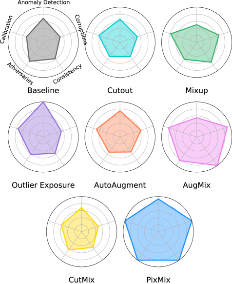
Figure 1: Normalized performance of different methods on five different model safety measures. PixMix is the only method that significantly outperforms the baseline in all five safety measures.

Ideally, models deployed in real-world settings would perform well on multiple safety measures. Unfortunately, prior work has shown that optimizing for some desirable properties often comes at the cost of others. For example, adversarial training only improves adversarial robustness and degrades classification performance [48]. Similarly, inducing consistent predictions on out-of-distribution (OOD) inputs seems to be at odds with better detecting these inputs, an intuition supported by recent work [4] which finds that existing help with some safety metrics but harm others. This raises the question of whether improving all safety measures is possible with a single model.

Method	Baseline	Cutout	Mixup	CutMix	PixMix
Corruptions mCE ($\downarrow$)	50.0 $+0.0$	51.5 $+1.5$	48.0 $-2.0$	51.5 $+1.5$	30.5 $\mathbf{-19.5}$
Adversaries Error ($\downarrow$)	96.5 $+0.0$	98.5 $+1.0$	97.4 $+0.9$	97.0 $+0.5$	92.9 $\mathbf{-3.9}$
Consistency mFR ($\downarrow$)	10.7 $+0.0$	11.9 $+1.2$	9.5 $-1.2$	12.0 $+1.3$	5.7 $\mathbf{-5.0}$
Calibration RMS Error ($\downarrow$)	31.2 $+0.0$	31.1 $-0.1$	13.0 $-18.1$	29.3 $-1.8$	8.1 $\mathbf{-23.0}$
Anomaly Detection AUROC ($\uparrow$)	77.7 $+0.0$	74.3 $-3.4$	71.7 $-6.0$	74.4 $-3.3$	$\mathbf{89.3}$ $\mathbf{+11.6}$

Table 1: PixMix comprehensively improves safety measures, providing significant improvements over state-of-the-art baselines. We observe that previous augmentation methods introduce few additional sources of structural complexity. By contrast, PixMix incorporates fractals and feature visualizations into the training process, actively exposing models to new sources of structural complexity. We find that PixMix is able to improve both robustness and uncertainty estimation and is the first method to substantially improve all existing safety measures over the baseline.

While previous augmentation methods create images that are different (e.g., translations) or more entropic (e.g., additive Gaussian noise), we argue that an important underexplored axis is creating images that are more complex. As opposed to entropy or descriptive difficulty, which is maximized by pure noise distributions, structural complexity is often described in terms of the degree of organization [28]. A classic example of structurally complex objects is fractals, which have recently proven useful for pretraining image classifiers [22, 35]. Thus, an interesting question is whether sources of structural complexity can be leveraged to improve safety through data augmentation techniques.

We show that Pareto improvements are possible with PixMix, a simple and effective data processing method that leverages pictures with complex structures and substantially improves all existing safety measures. PixMix consists of a new data processing pipeline that incorporates structurally complex “dreamlike” images. These dreamlike images include fractals and feature visualizations. We find that feature visualizations are a suitable source of complexity, thereby demonstrating that they have uses beyond interpretability. In extensive experiments, we find that PixMix provides substantial gains on a broad range of existing safety measures, outperforming numerous previous methods. Code is available at github.com/andyzoujm/pixmix.

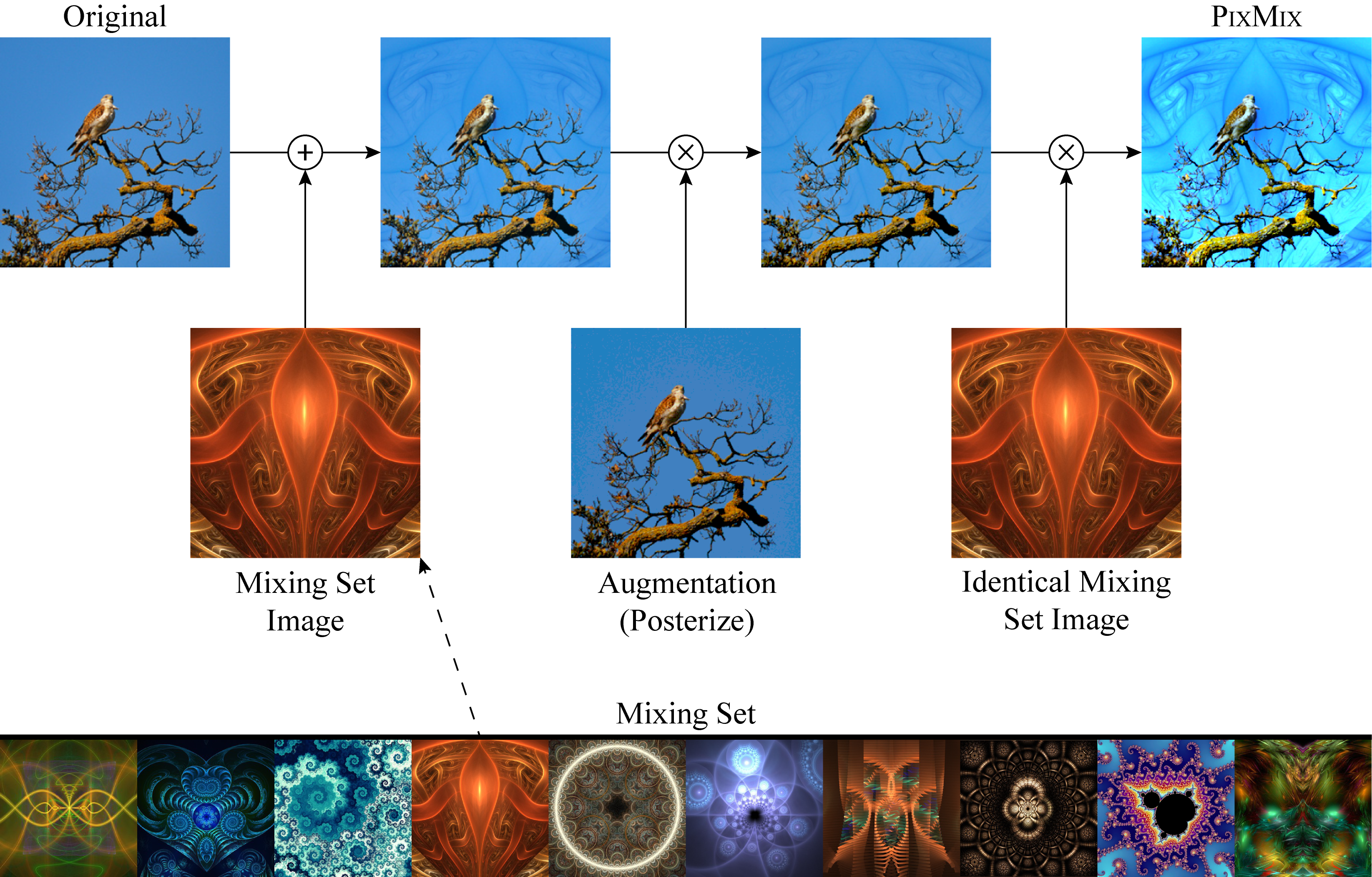
Figure 2: Top: An instance of a PixMix augmentation being applied to a bird image. The original clean image is mixed with augmented versions of itself and an image such as a fractal. Bottom: Sample images from the PixMix mixing set. We select fractals and feature visualizations from manually curated online sources. In ablations, we find that these new sources of visual structure for augmentations outperform numerous synthetic image distributions explored in prior work [2].

2 Related Work

Robustness. Out-of-distribution robustness considers how to make ML models resistant to various forms of data shift at test time. Geirhos et al., 2019 [11] uncover a texture bias in convolutional networks and show that training on diverse stylized images can improve robustness at test-time. The ImageNet-C(orruptions) benchmark [15] consists of diverse image corruptions known to track robustness on some real world data shifts [13]. ImageNet-C is used to test models that are trained on ImageNet [7] and is used as a held-out, more difficult test set. They also introduce ImageNet-P(erturbations) for measuring prediction consistency under various non-adversarial input perturbations. Others have introduced additional corruptions for evaluation called ImageNet-$\overline{\text{C}}$ [33]. The ImageNet-R(enditions) benchmark measures performance degradation under various renditions of objects including paintings, cartoons, graffiti, embroidery, origami, sculptures, toys, and more [13]. In the similar setting of domain adaptation, Bashkirova et al., 2021 [3] consider evaluating test-time robustness of models and even anomaly detection [10, 27, 41]. Yin et al., 2019 [50] show that adversarial training can substantially reduce robustness on some corruptions and argue that part of model fragility is explained by overreliance on spurious cues [43, 23].

Calibration. Calibrated prediction confidences are valuable for classification models in real-world settings. Several works have investigated evaluating and improving the calibration of deep neural networks [37, 12] through the use of validation sets. Others have shown that calibration can be improved without a validation set through methods such as ensembling [24] and pre-training [17]. Ovadia et al. [40] find that models are markedly less calibrated under distribution shift.

Anomaly Detection. Since models should ideally know what they do not know, they will need to identify when an example is anomalous. Anomaly detection seeks to estimate whether an input is out-of-distribution (OOD) with respect to a given training set. Hendrycks et al., 2017 [16] propose a simple baseline for detecting classifier errors and OOD inputs. Devries et al., 2018 [9] propose training classifiers with an additional confidence branch for detecting OOD inputs. Lee et al., 2018 [25] propose improving representations used for detectors with near-distribution images generated by GANs. Lee et al., 2018 [26] also propose the Mahalanobis detector. Outlier Exposure [18] fine-tunes classifiers with diverse, natural anomalies, and since it is the state-of-the-art for OOD detection, we test this method in our paper.

Data Augmentation. Simulated and augmented inputs can help make ML systems more robust, and this approach is used in real-world applications such as autonomous driving [46, 1]. For state-of-the-art models, data augmentation can improve clean accuracy comparably to a $10\times$ increase in model size [44]. Further, data augmentation can improve out-of-distribution robustness comparably to a $1,\!000\times$ increase in labeled data [13]. Various augmentation techniques for image data have been proposed, including Cutout [8, 55], Mixup [54, 47], CutMix [52, 45], and AutoAugment [6, 50]. Lopes et al., 2019 [29] find that inserting random noise patches into training images improves robustness. AugMix is a data augmentation technique that specifically improves OOD generalization [21]. Chun et al. [4] evaluates some of these techniques on CIFAR-10-C, a variant of ImageNet-C for the CIFAR-10 dataset [15]. They find that these data augmentation techniques can improve OOD generalization at the cost of weaker OOD detection.

Analyzing Safety Goals Simultaneously. Recent works study how a given method influences safety goals [14] simultaneously. Prior work has shown that Mixup, CutMix, Cutout, ShakeDrop, adversarial training, Gaussian noise augmentation, and more have mixed effects on various safety metrics [4]. Others have shown that different pretraining methods can improve some safety metrics and hardly affect others, but the pretraining method must be modified per task [17]. Self-supervised learning methods can also be repurposed to help with some safety goals, all while not affecting others, but to realize the benefit, each task requires different self-supervised learning models [20]. Thus, creating a single method for improving performance across multiple safety metrics is an important next step.

⬇

def pixmix(|$x_\text{orig}$|, |$x_\text{mixing\_pic}$|, k=4, beta=3):

|$x_\text{pixmix}$| = random.choice([|\color{blue}{augment}|(|$x_\text{orig}$|), |$x_\text{orig}$|])

\parfor i in range(random.choice([0,1,…,k])): # random count of mixing rounds

\par# mixing_pic is from the mixing set (e.g., fractal, natural image, etc.)

mix_image = random.choice([|\color{blue}{augment}|(|$x_\text{orig}$|), |$x_\text{mixing\_pic}$|])

mix_op = random.choice([additive, multiplicative])

\par|$x_\text{pixmix}$| = mix_op(|$x_\text{pixmix}$|, mix_image, beta)

\parreturn |$x_\text{pixmix}$|

\pardef augment(x):

aug_op = random.choice([rotate, solarize, …, posterize])

return aug_op(x)

Figure 3: Simplified code for PixMix, our proposed data augmentation method. Initial images are mixed with a randomly selected image from our mixing set or augmentations of the clean image. The mixing operations are selected at random, and the mixing set includes fractals and feature visualization pictures. PixMix integrates new complex structures into the training process by leveraging fractals and feature visualizations, resulting in improved classifier robustness and uncertainty estimation across numerous safety measures.

Training on Complex Synthetic Images. Kataoka et al., 2020 [22] introduce FractalDB, a dataset of black-and-white fractals, and they show that pretraining on these algorithmically generated fractal images can yield better downstream performance than pretraining on many manually annotated natural datasets. Nakashima et al. [35] show that models trained on a large variant of FractalDB can match ImageNet-1K pretraining on downstream tasks. Baradad et al., 2021 [2] find that, for self-supervised learning, other synthetic datasets may be more effective than FractalDB, and they find that structural complexity and diversity are key properties for good downstream transfer. We depart from this recent line of work and ask whether structurally complex images can be repurposed for data augmentation instead of training from scratch. While data augmentation techniques such as those that add Gaussian noise increase input entropy, such noise has maximal descriptive complexity but introduce little structural complexity [28]. Since a popular definition of structural complexity is the fractal dimension [28], we turn to fractals and other structurally complex images for data augmentation.

3 Approach

We propose PixMix, a simple and effective data augmentation technique that improves many ML Safety [14] measures simultaneously, in addition to accuracy. PixMix is comprised of two main components: a set of structurally complex pictures (“Pix”) and a pipeline for augmenting clean training pictures (“Mix”). At a high level, PixMix integrates diverse patterns from fractals and feature visualizations into the training set. As fractals and feature visualizations do not belong to any particular class, we train networks to classify augmented images as the original class, as in standard data augmentation.

3.1 Picture Sources (Pix)

While PixMix can utilize arbitrary datasets of pictures, we discover that fractals and feature visualizations are especially useful pictures with complex structures. Collectively we refer to these two picture sources as “dreamlike pictures.” We analyze PixMix using other picture sources in the Appendix.

These pictures have “non-accidental” properties that humans may use, namely “structural properties of contours (orientation, length, curvature) and contour junctions (types and angles) from line drawings of natural scenes” [49]. Fractals possess some of these structural properties, and they are highly non-accidental and unlikely to arise from maximum entropy, unstructured random noise processes.

Fractals. Fractals can be generated in several ways, with one of the most common being iterated function systems. Rather than generate our own diverse fractals, which is a substantial research endeavor [22], we download $14,\!230$ fractals from manually curated collections on DeviantArt. The resulting fractals are visually diverse, which can be seen in the bottom portion of Figure 2.

Feature Visualization. Feature visualizations that maximize the response of neurons create archetypal images for neurons and often have high complexity [34, 39]. Thus, we include feature visualizations in our mixing set. We collect $4,\!700$ feature visualizations from the initial layers of several convolutional architectures using OpenAI Microscope. While feature visualizations have been primarily used for understanding network representations, we connect this line of interpretability work to improve performance on safety measures.

3.2 Mixing Pipeline (Mix)

The pipeline for augmenting clean training images is described in Figure 3. An instance of our mixing pipeline is shown in the top half of Figure 2. First, a clean image has a $50\%$ chance of having a randomly selected standard augmentation applied. Next, we augment the image a random number of times with a maximum of $k$ times. Each augmentation is carried out by either additively or multiplicatively mixing the current image with a freshly augmented clean image or an image from the mixing set. Multiplicative mixing is performed similarly to the geometric mean. For both additive and multiplicative mixing, we use coefficients that are not convex combinations but rather conic combinations. Thus, additive and multiplicative mixing are performed with exponents and weights sampled from a Beta distribution independently.

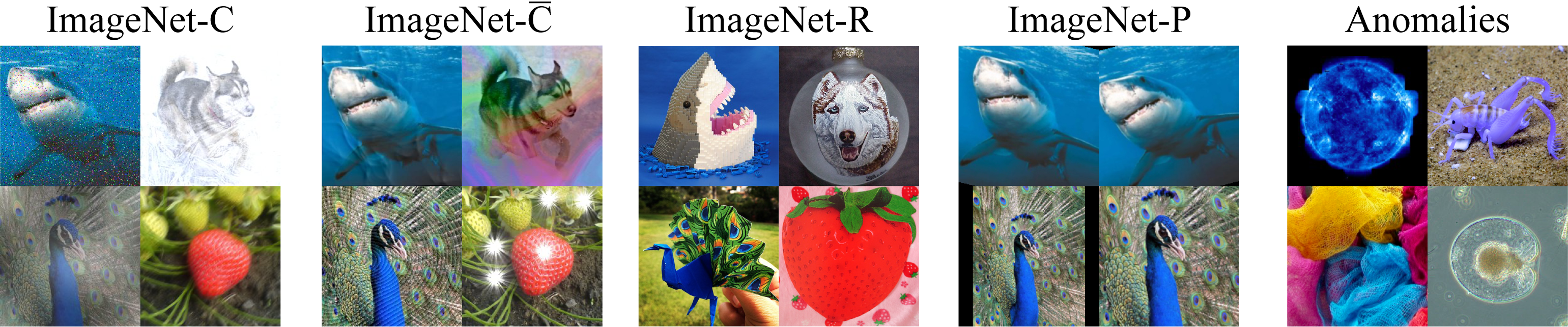
Figure 4: We comprehensively evaluate models across safety tasks, including corruption robustness (ImageNet-C, ImageNet-$\overline{\text{C}}$), rendition robustness (ImageNet-R), prediction consistency (ImageNet-P), confidence calibration, and anomaly detection. ImageNet-C [15] contains $15$ common corruptions, including fog, snow, and motion blur. ImageNet-$\overline{\text{C}}$ [33] contains additional corruptions. ImageNet-R [13] contains renditions of object categories and measures robustness to shape abstractions. ImageNet-P [15] contains sequences of gradual perturbations to images, across which predictions should be consistent. Anomalies are semantically distinct from the training classes. Existing work focuses on learning representations that improve performance on one or two metrics, often to the detriment of others. Developing models that perform well across multiple safety metrics is an important next step.

4 Experiments

Datasets. We evaluate PixMix on extensions of CIFAR-10, CIFAR-100, and ImageNet-1K (henceforth referred to as ImageNet) for various safety tasks. So as not to ignore performance on the original tasks, we also evaluate on the standard versions of these datasets. ImageNet consists of $1.28$ million color images. As is common practice, we downsample ImageNet images to $224\times 224$ resolution in all experiments. ImageNet consists of $1,\!000$ classes from WordNet noun synsets, covering a wide variety of objects, including fine-grained distinctions. We use the validation set for evaluating clean accuracy, which contains $50,\!000$ images.

To measure corruption robustness, we use the CIFAR-10-C, CIFAR-100-C, and ImageNet-C datasets [15]. Each dataset consists of $15$ diverse corruptions applied to each image in the original test set. The corruptions can be grouped into blur, weather, and digital corruptions. Each corruption appears at five levels of severity. We also evaluate on the similar CIFAR-10-$\mkern 1.5mu\overline{\mkern-1.5mu\text{C}\mkern-1.5mu}\mkern 1.5mu$ and ImageNet-$\mkern 1.5mu\overline{\mkern-1.5mu\text{C}\mkern-1.5mu}\mkern 1.5mu$ datasets, which use a different set of corruptions [33]. To measure robustness to different renditions of object categories, we use the ImageNet-R dataset [13]. These datasets enable evaluating the out-of-distribution generalization of classifiers trained on clean data and non-overlapping augmentations.

To measure consistency of predictions, we use the CIFAR-10-P, CIFAR-100-P, and ImageNet-P datasets. Each dataset consists of $10$ gradual shifts that images can undergo, such as zoom, translation, and brightness variation. Unlike other datasets we evaluate on, each example in these datasets is a video, and the objective is to have robust predictions that do not change across per-frame perturbations. These datasets enable measuring the stability, volatility, or “jaggedness” of network predictions in the face of minor perturbations. Examples from these datasets are in Figure 4.

Methods. We compare PixMix to various state-of-the-art data augmentation methods. Baseline denotes standard data augmentation; for ImageNet, we use the a random resized crop and random horizontal flipping, while on CIFAR-10 and CIFAR-100, we use random cropping with zero padding followed by random horizontal flips. Cutout aims to improve representations by randomly masking out image patches, using patch side lengths that are half the side length of the original image. Mixup regularizes networks to behave linearly between training examples by training on pixel-wise linear interpolations between input images and labels. CutMix combines the techniques of Cutout and Mixup by replacing image patches with patches from other images in the training set. The labels of the resulting images are combined in proportion to the pixels taken by each source image. Auto Augment searches for compositions of augmentations that maximize accuracy on a validation set. AugMix uses a ResNeXt-like pipeline to combine randomly augmented images. Compared to AugMix, which requires up to $9$ augmentations per image and can be slow to run, PixMix requires substantially fewer augmentations; we find an average of $2$ augmentations is sufficient. For fairness, we follow [33] and train AugMix without the Jensen-Shannon Divergence consistency loss, which requires at least thrice the memory per batch. Outlier Exposure trains networks to be uncertain on a training dataset of outliers, and these outliers are distinct from the out-of-distribution test sets that we use during evaluation. For ImageNet experiments, we compare to several additional methods. SIN trains networks on a mixture of clean images and images rendered using neural style transfer [11]. We opt for simple techniques that are widely used and do not evaluate all possible techniques from each of the areas we consider. More methods are evaluated in the Appendix.

		Baseline	Cutout	Mixup	CutMix	Auto Augment	AugMix	Outlier Exposure	PixMix
CIFAR-10	Corruptions	26.4	25.9	21.0	26.5	22.2	12.4	25.1	9.5
	Consistency	3.4	3.7	2.9	3.5	3.6	1.7	3.4	1.7
	Adversaries	91.3	96.0	93.3	92.1	95.1	86.8	92.9	82.1
	Calibration	22.7	17.8	12.1	18.6	14.8	9.4	13.0	3.7
	Anomaly Detection ($\uparrow$)	91.9	91.4	88.2	92.0	93.2	89.2	98.4	97.0
CIFAR-100	Corruptions	50.0	51.5	48.0	51.5	47.0	35.4	51.5	30.5
	Consistency	10.7	11.9	9.5	12.0	11.2	6.5	11.3	5.7
	Adversaries	96.8	98.5	97.4	97.0	98.1	95.6	97.2	92.9
	Calibration	31.2	31.1	13.0	29.3	24.9	18.8	15.2	8.1
	Anomaly Detection ($\uparrow$)	77.7	74.3	71.7	74.4	80.4	84.9	90.3	89.3

Table 2: On CIFAR-10 and CIFAR-100, PixMix outperforms state-of-the-art techniques on five distinct safety metrics. Lower is better except for anomaly detection, and full results are in the Supplementary Material. On robustness tasks and confidence calibration, PixMix outperforms all prior methods by significant margins. On anomaly detection, PixMix nearly matches the performance of the state-of-the-art Outlier Exposure method without requiring a large, diverse dataset of known outliers.

4.1 Tasks and Metrics

We compare PixMix to methods on five distinct ML Safety tasks. Individual methods are trained on clean versions of CIFAR-10, CIFAR-100, and ImageNet. Then, they are evaluated on each of the following tasks.

Corruptions. This task is to classify corrupted images from the CIFAR-10-C, CIFAR-100-C, and ImageNet-C datasets. The metric is the mean corruption error (mCE) across all fifteen corruptions and five severities for each corruption. Lower is better.

Consistency. This task is to consistently classify sequences of perturbed images from CIFAR-10-P, CIFAR-100-P, and ImageNet-P. The main metric is the mean flip rate (mFR), which corresponds to the probability that adjacent images in a temporal sequence have different predicted classes. This can be written as $\mathbb{P}_{x\sim\mathcal{S}}(f(x_{j})\neq f(x_{j-1}))$, where $x_{i}$ is the $i^{\text{th}}$ image in a sequence. For non-temporal sequences such as increasing noise values in a sequence $\mathcal{S}$, the metric is modified to $\mathbb{P}_{x\sim\mathcal{S}}(f(x_{j})\neq f(x_{1}))$. Lower is better.

Adversaries. This task is to classify images that have been adversarially perturbed by projected gradient descent [32]. For this task, we focus on untargeted perturbations on CIFAR-10 and CIFAR-100 with an $\ell_{\infty}$ budget of $2/255$ and $20$ steps of optimization. We do not display results of ImageNet models against adversaries in our tables, as for all tested methods the accuracy declines to zero with this budget. The metric is the classifier error rate. Lower is better.

Calibration. This task is to classify images with calibrated prediction probabilities, i.e. matching the empirical frequency of correctness. For example, if a weather forecast predicts that it will rain with $70\%$ probability on ten occasions, then we would like the model to be correct $7/10$ times. Formally, we want posteriors from a model $f$ to satisfy $\mathbb{P}\left(Y=\arg\max_{i}f(X)_{i}\mid\max_{i}f(X)_{i}=C\right)=C$, where $X,Y$ are random variables representing the data distribution. The metric is RMS calibration error [19], which is computed as $\sqrt{\mathbb{E}_{C}[(\mathbb{P}(Y=\hat{Y}|C=c)-c)^{2}]}$, where $C$ is the classifier’s confidence that its prediction $\hat{Y}$ is correct. We use adaptive binning [38] to compute this metric. Lower is better.

Anomaly Detection. In this task we detect out-of-distribution [16] or out-of-class images from various unseen distributions. The anomaly distributions are Gaussian, Rademacher, Blobs, Textures [5], SVHN [36], LSUN [51], Places69 [56]. We describe each in the Appendix and report average AUROC. An AUROC of $50\%$ is random chance and $100\%$ is perfect detection. Higher is better.

4.2 Results on CIFAR-10/100 Tasks

Training Setup. In the following CIFAR experiments, we train a 40-4 Wide ResNet [53] with a drop rate of $0.3$ for $100$ epochs. All experiments use an initial learning rate of $0.1$ which decays following a cosine learning rate schedule [30]. For PixMix experiments, we use $k=4,\beta=3$. Hyperparameter robustness is discussed in the Appendix. Additionally, we use a weight decay of $0.0001$ for Mixup and $0.0005$ otherwise.

	Accuracy	Robustness			Consistency		Calibration				Anomaly Detection
	Clean	C	$\overline{\text{C}}$	R	ImageNet-P		Clean	C	$\overline{\text{C}}$	R	Out-of-Class Datasets
	Error	mCE	Error	Error	mFR	mT5D	RMS	RMS	RMS	RMS	AUROC ($\uparrow$)	AUPR ($\uparrow$)
Baseline	23.9	78.2	61.0	63.8	58.0	78.4	5.6	12.0	20.7	19.7	79.7	48.6
Cutout	22.6	76.9	60.2	64.8	57.9	75.2	3.8	11.1	17.1	14.6	81.7	49.6
Mixup	22.7	72.7	55.0	62.3	54.3	73.2	5.8	7.3	13.2	44.6	72.2	51.3
CutMix	22.9	77.8	59.8	66.5	60.3	76.6	6.2	9.1	15.3	43.5	78.4	47.9
AutoAugment	22.4	73.8	58.0	61.9	54.2	72.0	3.6	8.0	14.3	12.6	84.4	58.2
AugMix	22.8	71.0	56.5	61.7	52.7	70.9	4.5	9.2	15.0	13.2	84.2	61.1
SIN	25.4	70.9	57.6	58.5	54.4	71.8	4.2	6.5	14.0	16.2	84.8	62.3
PixMix	22.6	65.8	44.3	60.1	51.1	69.1	3.6	6.3	5.8	11.0	85.7	64.1

Table 3: On ImageNet, PixMix improves over state-of-the-art methods on a broad range of safety metrics. Lower is better except for anomaly detection, and the full results are in the Supplementary Material. Bold is best, and underline is second best. Across evaluation settings, PixMix is occasionally second-best, but it is usually first, making it near Pareto-optimal.

Results. In Table 1, we see that PixMix improves over the standard baseline method on all safety measures. Moreover, all other methods decrease performance relative to the baseline for at least one metric, while PixMix is the first method to improve performance in all settings. Results for all other methods are in Table 2. PixMix obtains better performance than all methods on Corruptions, Consistency, Adversaries, and Calibration. Notably, PixMix is far better than other methods for improving confidence calibration, reaching acceptably low calibration error on CIFAR-10. For corruption robustness, performance improvements on CIFAR-100 are especially large, with mCE on the Corruptions task dropping by $4.9\%$ compared to AugMix and $19.5\%$ compared to the baseline.

In addition to robustness and calibration, PixMix also greatly improves anomaly detection. PixMix nearly matches the anomaly detection performance of Outlier Exposure, the state-of-the-art anomaly detection method, without requiring large quantities of diverse, known outliers. This is surprising, as PixMix uses a standard cross-entropy loss, which makes the augmented images seem more in-distribution. Hence, one might expect unseen corruptions to be harder to distinguish as well, but in fact we observe the opposite—anomalies are easier to distinguish. Additional results and ablations are in the Appendix.

		Accuracy	Corruptions	Consistency	Adversaries	Calibration	Anomaly
		Clean	C	CIFAR-P	PGD	C	Detection
	PixMix Mixing Set	Error	mCE	mFR	Error	RMS	AUROC ($\uparrow$)
Previous	Dead Leaves (Squares) [2]	21.3	36.2	6.3	94.1	15.8	81.8
	Spectrum + Color + WMM [2]	20.7	36.1	6.6	94.4	15.9	85.8
	StyleGAN (Oriented) [2]	20.4	37.3	7.2	97.0	14.9	83.7
	FractalDB [22]	20.3	33.9	6.4	98.2	12.0	82.5
	300K Random Images [19]	19.6	34.5	6.3	94.7	12.9	86.2
1-8 New	Fractals	20.3	32.3	6.2	95.5	8.7	88.9
	Feature Visualization (FVis)	21.5	30.3	5.4	91.5	9.9	88.1
	Fractals + FVis	20.3	30.5	5.7	92.9	8.1	89.3

Table 4: Mixing set ablations showing that PixMix can use numerous mixing sets, including real images. Results are using CIFAR-100. Bold is best, and underline is second best. We compare Fractals + FVis, the mixing set used as PixMix’s default mixing set, to other datasets from prior work. The 300K Random Images are real images scraped from online for Outlier Exposure. We discover the distinct utility of Fractals and FVis. By utilizing the 300K Random Images mixing set, PixMix can attain a $19.6\%$ error rate, though fractals can provide more robustness than these real images.

4.3 Results on ImageNet Tasks

Training Setup. Since regularization methods may require a greater number of training epochs to converge, we fine-tune a pre-trained ResNet-50 for 90 epochs. For PixMix experiments, we use $k=4,\beta=4$. We use a batch size of $512$ and an initial learning rate of $0.01$ following a cosine decay schedule.

Results. We show ImageNet results in Table 3. Compared to the standard augmentations of the baseline, PixMix has higher performance on all safety measures. By contrast, other augmentation methods have lower performance than the baseline (cropping and flipping) on some metrics. Thus, PixMix is the first augmentation method with a Pareto improvement over the baseline on a broad range of safety measures.

On corruption robustness, PixMix outperforms state-of-the-art augmentation methods such as AugMix, improving mCE by $12.4\%$ over the baseline and $5.1\%$ over the mCE of the next-best method. On rendition robustness, PixMix outperforms all other methods save for SIN. Note that SIN is particularly well-suited to improving rendition robustness, as it trains on stylized ImageNet data. However, SIN incurs a $2\%$ loss to clean accuracy, while PixMix increases clean accuracy by $1.3\%$. Maintaining strong performance on clean images is an important property for methods to have, as practitioners may be unwilling to adopt methods that markedly reduce performance in ideal conditions.

On calibration tasks, PixMix outperforms all methods. As Ovadia et al. [40] show, models are markedly less calibrated under distribution shift. We find that PixMix cuts calibration error in half on ImageNet-C compared to the baseline. On ImageNet-$\mkern 1.5mu\overline{\mkern-1.5mu\text{C}\mkern-1.5mu}\mkern 1.5mu$, the improvement is even larger, with a $14.9\%$ reduction in absolute error. In Figure 5, we visualize how calibration error on ImageNet-C and ImageNet-$\mkern 1.5mu\overline{\mkern-1.5mu\text{C}\mkern-1.5mu}\mkern 1.5mu$ varies as the corruption severities increase. Compared to the baseline, PixMix calibration error increases much more slowly. Further uncertainty estimation results are in the Appendix. For example, PixMix substantially improves anomaly detection performance with Places365 as the in-distribution set.

4.4 Mixing Set Picture Source Ablations

While we provide a high-quality source of structural complexity with PixMix, our mixing pipeline could be used with other mixing sets. In Table 4, we analyze the choice of mixing set on CIFAR-100 performance. We replace our Fractals and Feature Visualizations dataset (Fractals + FVis) with several synthetic datasets developed for unsupervised representation learning [2, 22]. We also evaluate the 300K Random Images dataset of natural images used for Outlier Exposure on CIFAR-10 and CIFAR-100 [19].

Compared to alternative sources of visual structure, the Fractals + FVis mixing set yields substantially better results. This suggests that structural complexity in the mixing set is important. Indeed, the next-best method for reducing mCE on CIFAR-100-C is FractalDB, which consists of weakly curated black-and-white fractal images. By contrast, our Fractals dataset consists of color images of fractals that were manually designed and curated for being visually interesting. Furthermore, we find that removing either Fractals or FVis from the mixing set yields lower performance on safety metrics or lower performance on clean data, showing that both components of our mixing set are important. Similar ablations on ImageNet shown in Table 10 follow the same trend.

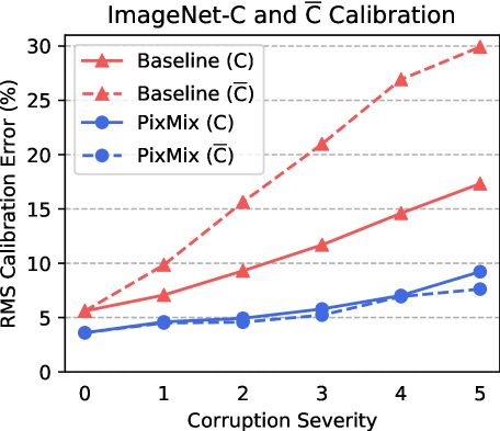
Figure 5: As corruption severity increases, PixMix calibration error increases much more slowly than the baseline calibration error, demonstrating that PixMix can improve uncertainty estimation under distribution shifts with unseen image corruptions.

5 Conclusion

We proposed PixMix, a simple and effective data augmentation technique for improving ML safety measures. Unlike previous data augmentation techniques, PixMix introduces new complexity into the training procedure by leveraging fractals and feature visualizations. We evaluated PixMix on numerous distinct ML Safety tasks: corruption robustness, rendition robustness, prediction consistency, adversarial robustness, confidence calibration, and anomaly detection. We found that PixMix was the first method to provide substantial improvements over the baseline on all existing safety metrics, and it obtained state-of-the-art performance in nearly all settings.

Appendix A Additional Results

Mixing Strategies.

In Table 5, we analyze different mixing strategies. The full PixMix mixing strategy is depicted in Figures 2 and 3 of the main paper. Mix Input only includes clean images in the mixing pipeline and does not use the mixing set at all. This severely harms performance on all safety metrics. Mix Aug only mixes with images from the mixing set. This reduces RMS calibration error but increases error on robustness tasks compared to PixMix Original. Finally, Iterative mixes with feature visualizations computed on the fly for the network being trained. This performs well on robustness tasks but has weaker calibration and anomaly detection. Additionally, computing feature visualizations at each iteration of training is substantially slower than precomputing them on fixed networks as we do in PixMix.

Full Results.

In Tables 7, 8, and 9, we report full results for CIFAR-10, CIFAR-100, and ImageNet. The ImageNet results are copied from the main paper. For CIFAR, we evaluate on additional datasets, including CIFAR-10-$\mkern 1.5mu\overline{\mkern-1.5mu\text{C}\mkern-1.5mu}\mkern 1.5mu$ and CIFAR-100-$\mkern 1.5mu\overline{\mkern-1.5mu\text{C}\mkern-1.5mu}\mkern 1.5mu$, additional datasets of corrupted CIFAR images. We also report the mT5D metric on ImageNet-P. In all cases, PixMix provides the best overall performance.

Noise-Based Augmentations.

Since noise-based augmentations sometimes nearly overlap with the test distribution and thereby may have an unfair advantage, we separately compare to several additional baselines on ImageNet that use noise-based data augmentations. ANT trains networks on inputs with adversarially transformed noise applied [42]. Speckle trains on inputs with speckle noise added, which has been observed to improve robustness. EDSR and Noise2Net inject noise using image-to-image neural networks with noisy parameters [13]. Adversarial trains networks with $\ell_{\infty}$ perturbations of magnitude $\varepsilon=8/255$ [31].

Results are in Tables 11. We find that ANT and Speckle have strong performance on ImageNet-P overall, but this mostly comes from the Gaussian and shot noise categories. If we only consider prediction stability on non-noise categories, PixMix exhibits the least volatility in predictions out of all the methods considered.

Hyperparameter Sensitivity.

In Table 14, we examine the hyperparameter sensitivity of PixMix on corruption robustness for CIFAR-100. We vary the $\beta$ and $k$ hyperparameters and find that performance is very stable across a range of hyperparameters.

Places365 Anomaly Detection.

In Table 13, we show anomaly detection performance with Places365 as the in-distribution data. For all methods, we use a ResNet-18 pre-trained on Places365. PixMix and Outlier Exposure (OE) are fine-tuned for $10$ epochs. We find that PixMix nearly matches the state-of-the-art OE detector despite being a general data augmentation technique that improves many other safety metrics.

Appendix B Outlier Datasets

For anomaly detection, we use a suite of out-of-distribution datasets and average metrics across all OOD datasets in the main results. Gaussian noise is IID noise sampled from a normal distribution. Rademacher Noise is noise with each pixel sampled from $\{-1,1\}$ with equal probability. Blobs are algorithmically generated blobs. Textures are from the Describable Textures Dataset [5]. SVHN has images of numbers from houses. Places69 contains 69 scene categories and is disjoint from Places365.

Appendix C Broader Impacts

As PixMix differentially improves safety metrics, it could have various beneficial effects. Improved robustness can result in more reliable machine learning systems deployed in safety-critical situations [14], such as self-driving cars. Anomaly detection enables better human oversight of machine learning systems and fallback policies in cases where systems encounter inputs they were not designed to handle. At the same time, anomaly detection could be misused as a surveillance tool, requiring careful consideration of individual use cases. Calibration enables more meaningful predictions that increase trust with end users. Additionally, compared to other methods for improving robustness, PixMix requires minimal modification of the training setup and a low computational overhead, resulting in lower costs to machine learning practitioners and the environment.

	Accuracy	Corruptions	Consistency	Adversaries	Calibration	Anomaly
	Clean	C	CIFAR-P	PGD	C	Detection
	Error ($\downarrow$)	mCE ($\downarrow$)	mFR ($\downarrow$)	Error ($\downarrow$)	RMS ($\downarrow$)	AUROC ($\uparrow$)
PixMix Original	20.3	30.5	5.7	92.9	8.1	89.3
Mix Input	19.9	34.1	6.4	96.7	15.5	86.5
Mix Aug	20.6	31.1	6.2	94.2	6.0	89.7
Iterative	21.1	31.4	5.6	90.6	12.7	86.7

Table 5: PixMix variations on CIFAR-100. Mix Input only mixes with augmented versions of the clean image. Mix Aug only mixes with images from the mixing set (i.e. fractals and feature visualizations). Iterative mixes with feature visualizations computed on the fly for the current network. Using the mixing set alone is more effective than augmented images alone, and combining them can further improve performance on several metrics.

	Accuracy	Corruptions		Consistency		Adversaries	Calibration			Anomaly
	Clean	C	$\overline{\text{C}}$	CIFAR-P		PGD	Clean	C	$\overline{\text{C}}$	Detection
	Error	mCE	mCE	mFR	mT5D	Error	RMS	RMS	RMS	AUROC ($\uparrow$)	AUPR ($\uparrow$)
CutMix	20.3	51.5	49.6	12.0	3.0	97.0	12.2	29.3	26.5	74.4	32.3
PixMix	20.3	30.5	36.7	5.7	1.6	92.9	7.0	8.1	8.9	89.3	70.9
PixMix + CutMix	19.9	30.9	35.5	5.8	1.7	93.1	4.4	6.0	5.9	89.5	68.6

Table 6: Combining PixMix and CutMix on CIFAR-100. While PixMix is strong on its own, combination with other data augmentation techniques can further improve performance.

	Accuracy	Corruptions		Consistency		Adversaries	Calibration			Anomaly
	Clean	C	$\overline{\text{C}}$	CIFAR-P		PGD	Clean	C	$\overline{\text{C}}$	Detection
	Error	mCE	mCE	mFR	mT5D	Error	RMS	RMS	RMS	AUROC ($\uparrow$)	AUPR ($\uparrow$)
Baseline	21.3	50.0	52.0	10.7	2.7	96.8	14.6	31.2	30.9	77.7	35.4
Cutout	19.9	51.5	50.2	11.9	2.7	98.5	11.4	31.1	29.4	74.3	31.3
Mixup	21.1	48.0	49.8	9.5	3.0	97.4	10.5	13.0	12.9	71.7	31.9
CutMix	20.3	51.5	49.6	12.0	3.0	97.0	12.2	29.3	26.5	74.4	32.3
AutoAugment	19.6	47.0	46.8	11.2	2.6	98.1	9.9	24.9	22.8	80.4	33.2
AugMix	20.6	35.4	41.2	6.5	1.9	95.6	12.5	18.8	22.5	84.9	53.8
OE	21.9	50.3	52.1	11.3	3.0	97.0	12.0	13.8	13.9	90.3	66.2
PixMix	20.3	30.5	36.7	5.7	1.6	92.9	7.0	8.1	8.9	89.3	70.9

Table 7: Full results for CIFAR-100. mT5D is an additional metric used for gauging prediction consistency in ImageNet-P, which we adapt to CIFAR-100. Note PixMix can achieve 19.6% error rate if it uses 300K Random Images as the Mixing Set, so PixMix can achieve the same accuracy as AutoAugment yet also do better on safety metrics.

	Accuracy	Corruptions		Consistency		Adversaries	Calibration			Anomaly
	Clean	CIFAR-C	$\overline{\text{C}}$	CIFAR-P		PGD	Clean	CIFAR-C	$\overline{\text{C}}$	Detection
	Error	mCE	mCE	mFR	mT5D	Error	RMS	RMS	RMS	AUROC ($\uparrow$)	AUPR ($\uparrow$)
Baseline	4.4	26.4	26.4	3.4	1.7	91.3	6.4	22.7	22.4	91.9	70.9
Cutout	3.6	25.9	24.5	3.7	1.7	96.0	3.3	17.8	17.5	91.4	63.6
Mixup	4.2	21.0	22.1	2.9	2.1	93.3	12.5	12.1	10.9	88.2	67.1
CutMix	4.0	26.5	25.4	3.5	2.1	92.1	5.0	18.6	17.8	92.0	65.5
AutoAugment	3.9	22.2	24.4	3.6	1.7	95.1	4.0	14.8	16.6	93.2	64.6
AugMix	4.3	12.4	16.4	1.7	1.2	86.8	5.1	9.4	12.6	89.2	61.5
OE	4.6	25.1	26.1	3.4	1.9	92.9	6.9	13.0	13.2	98.4	92.5
PixMix	4.2	9.5	13.6	1.7	1.0	82.1	2.6	3.7	5.3	97.0	88.4

Table 8: Full results for CIFAR-10. mT5D is an additional metric used for gauging prediction consistency in ImageNet-P, which we adapt to CIFAR-10.

	Accuracy	Robustness			Consistency		Calibration				Anomaly
	Clean	C	$\overline{\text{C}}$	R	ImageNet-P		Clean	C	$\overline{\text{C}}$	R	Detection
	Error	mCE	Error	Error	mFR	mT5D	RMS	RMS	RMS	RMS	AUROC ($\uparrow$)	AUPR ($\uparrow$)
Baseline	23.9	78.2	61.0	63.8	58.0	78.4	5.6	12.0	20.7	19.7	79.7	48.6
Cutout	22.6	76.9	60.2	64.8	57.9	75.2	3.8	11.1	17.1	14.6	81.7	49.6
Mixup	22.7	72.7	55.0	62.3	54.3	73.2	5.8	7.3	13.2	44.6	72.2	51.3
CutMix	22.9	77.8	59.8	66.5	60.3	76.6	6.2	9.1	15.3	43.5	78.4	47.9
AutoAugment	22.4	73.8	58.0	61.9	54.2	72.0	3.6	8.0	14.3	12.6	84.4	58.2
AugMix	22.8	71.0	56.5	61.7	52.7	70.9	4.5	9.2	15.0	13.2	84.2	61.1
SIN	25.4	70.9	57.6	58.5	54.4	71.8	4.2	6.5	14.0	16.2	84.8	62.3
PixMix	22.6	65.8	44.3	60.1	51.1	69.1	3.6	6.3	5.8	11.0	85.7	64.1

Table 9: Full results for ImageNet. mT5D is an additional metric used for gauging prediction consistency in ImageNet-P. Bold is best, and underline is second best.

	Accuracy	Robustness			Consistency		Calibration				Anomaly
	Clean	C	$\overline{\text{C}}$	R	ImageNet-P		Clean	C	$\overline{\text{C}}$	R	Detection
	Error	mCE	Error	Error	mFR	mT5D	RMS	RMS	RMS	RMS	AUROC ($\uparrow$)	AUPR ($\uparrow$)
Baseline	23.9	78.2	61.0	63.8	58.0	78.4	5.6	12.0	20.7	19.7	79.7	48.6
Fractals	22.0	68.2	47.4	60.6	52.6	71.1	4.0	7.2	7.4	11.7	85.3	62.6
ResNet only FVis	22.1	64.3	45.3	60.1	50.7	69.1	3.9	7.1	7.6	12.2	85.1	63.3
Fractals + FVis	22.6	65.8	44.3	60.1	51.1	69.1	3.6	6.3	5.8	11.0	85.7	64.1

Table 10: Similar to the results obtained in CIFAR-100 mixing set ablations, a fractal-only mixing set is effective (Fractals), but combining fractals and feature visualizations yields the best performance (Fractals + FVis). Moreover, feature visualizations from a model trained with the same dataset and architecture perform well (ResNet only FVis), showing that knowledge distillation does not explain the results.

	Accuracy	Robustness			Consistency		Calibration				Anomaly
	Clean	C	$\overline{\text{C}}$	R	ImageNet-P		Clean	C	$\overline{\text{C}}$	R	Detection
	Error	mCE	Error	Error	mFR	mT5D	RMS	RMS	RMS	RMS	AUROC ($\uparrow$)	AUPR ($\uparrow$)
Baseline	23.9	78.2	61.0	63.8	58.0	78.4	5.6	12.0	20.7	19.7	79.7	48.6
ANT	23.9	67.0	61.0	61.0	48.0	68.4	7.0	10.3	19.3	22.9	80.9	54.3
Speckle	24.2	72.7	62.1	62.1	51.2	70.6	5.6	11.6	19.8	20.9	79.7	53.3
Noise2Net	22.7	71.6	57.7	57.6	51.5	72.3	4.4	8.9	16.3	15.2	84.8	60.4
EDSR	23.5	65.4	54.7	60.3	44.6	63.3	4.5	8.4	15.7	16.7	71.7	36.3
$\ell_{\infty}$ Adversarial	45.5	92.6	68.0	65.2	38.5	41.5	15.5	10.2	15.1	10.2	69.8	26.4
$\ell_{2}$ Adversarial	37.2	85.5	64.9	63.0	29.2	34.8	11.3	9.7	16.6	10.7	78.9	40.2

Table 11: While many noise-based augmentation methods often do well on ImageNet-C by targeting the noise corruptions, they do not reliably improve performance across many safety metrics.

			Noise		Blur		Weather		Digital
	Clean	mFR	Gaussian	Shot	Motion	Zoom	Snow	Bright	Translate	Rotate	Tilt	Scale
Baseline	23.9	58.0	59	58	65	72	63	62	44	52	57	48
ANT	23.9	48.0	41	36	50	61	48	58	40	48	52	46
Speckle	24.2	51.2	38	28	60	67	58	65	43	51	54	48
Noise2Net	22.7	51.5	54	53	50	70	56	50	38	47	52	43
EDSR	23.5	44.6	37	35	48	56	46	56	38	44	44	43
$\ell_{\infty}$ Adversarial	45.5	38.5	43	56	24	33	15	80	20	34	33	46
$\ell_{2}$ Adversarial	37.2	29.2	24	30	24	31	14	64	13	27	26	39

Table 12: ImageNet-P results. The mean flipping rate is the average of the flipping rates across all 10 perturbation types. Noise-based augmentation methods are less performant on non-noise distribution shifts.

	AUROC ($\uparrow$)			AUPR ($\uparrow$)
	Baseline	OE	PixMix	Baseline	OE	PixMix
Gaussian Noise	72.2	93.5	100.0	23.5	54.1	100.0
Rademacher Noise	47.7	90.2	100.0	14.6	44.9	100.0
Blobs	41.9	100.0	100.0	13.0	99.4	100.0
Textures	66.6	91.4	80.3	24.6	75.7	56.2
SVHN	96.6	100.0	99.5	90.5	99.9	98.6
ImageNet	63.0	86.5	71.5	25.1	69.7	47.4
Places69	61.5	63.1	62.3	23.4	24.9	31.3
Average	64.2	89.2	87.6	30.7	66.9	76.2

Table 13: Out-of-Distribution detection results for a ResNet-18 pre-trained on Places365. PixMix and OE are finetuned for 10 epochs. Despite being a general data augmentation technique, PixMix is near the state-of-the-art in OOD detection.

	$k=2$	$k=3$	$k=4$
$\beta=5$	20.2 31.6	20.0 31.1	20.1 30.8
$\beta=4$	19.7 31.3	20.3 30.9	20.1 30.7
$\beta=3$	20.3 31.2	20.2 30.7	20.3 30.5

Table 14: Performance is not strongly affected by hyperparameters. We include the CIFAR-100 test set error and the CIFAR-100-C mCE for each hyperparameter setting.

			Noise			Blur				Weather				Digital
	Clean	mCE	Gauss.	Shot	Impulse	Defocus	Glass	Motion	Zoom	Snow	Frost	Fog	Bright	Contrast	Elastic	Pixel	JPEG
Baseline	23.9	78.2	78	80	80	79	90	81	80	80	78	69	62	75	88	76	78
Cutout	22.6	76.9	76	77	79	76	90	79	79	79	78	69	60	74	87	75	75
Mixup	22.7	72.7	69	72	73	76	90	77	78	73	68	62	59	64	86	71	73
CutMix	22.9	77.8	78	80	80	79	90	81	80	80	78	69	62	75	88	76	78
AutoAugment	22.4	73.8	71	72	75	75	90	78	79	73	74	64	55	68	87	73	71
AugMix	22.8	71.0	69	70	70	72	88	74	71	73	74	58	58	59	85	73	72
SIN	25.4	70.9	64	65	66	73	84	73	80	71	74	66	62	69	80	64	73
PixMix	22.6	65.8	53	52	51	73	88	77	77	62	64	58	56	53	85	69	70

Table 15: Clean Error, mCE, and Corruption Error (CE) values for various methods on ImageNet-C. The mCE value is computed by averaging across per corruption CE values.

	Clean	$\overline{\text{C}}$ Error	Blue Sample	Plasma	Checkerboard	Cocentric Sine	Single Freq	Brown	Perlin	Sparkles	Inverse Sparkle	Refraction
Baseline	23.9	61.0	62	77	55	86	80	45	41	38	78	48
Cutout	22.6	60.2	64	77	49	85	80	45	41	36	77	47
Mixup	22.7	55.0	58	68	49	80	72	38	36	35	71	44
CutMix	22.9	59.8	64	77	47	85	80	46	41	35	75	47
AutoAugment	22.4	58.0	56	71	49	86	77	42	39	36	77	47
AugMix	22.8	56.5	51	71	48	83	76	42	38	36	75	45
SIN	25.4	57.6	53	72	54	81	68	41	41	41	79	47
PixMix	22.6	44.3	40	48	48	48	47	34	37	33	65	44

Table 16: Results for various methods on ImageNet-$\overline{\text{C}}$.

References

- [1] Drago Anguelov. Machine learning for autonomous driving, 2019.
- [2] Manel Baradad, Jonas Wulff, Tongzhou Wang, Phillip Isola, and Antonio Torralba. Learning to see by looking at noise. arXiv preprint arXiv:2106.05963, 2021.
- [3] Dina Bashkirova, Dan Hendrycks, Donghyun Kim, Samarth Mishra, Kate Saenko, Kuniaki Saito, Piotr Teterwak, and Ben Usman. Visda-2021 competition universal domain adaptation to improve performance on out-of-distribution data. arXiv preprint arXiv:2107.11011, 2021.
- [4] Sanghyuk Chun, Seong Joon Oh, Sangdoo Yun, Dongyoon Han, Junsuk Choe, and Youngjoon Yoo. An empirical evaluation on robustness and uncertainty of regularization methods. Uncertainty and Robustness in Deep Learning. ICML Workshop, 2019.
- [5] M. Cimpoi, S. Maji, I. Kokkinos, S. Mohamed, , and A. Vedaldi. Describing textures in the wild. In Computer Vision and Pattern Recognition, 2014.
- [6] Ekin Dogus Cubuk, Barret Zoph, Dandelion Mané, Vijay Vasudevan, and Quoc V. Le. AutoAugment: Learning augmentation policies from data. CVPR, 2018.
- [7] Jia Deng, Wei Dong, Richard Socher, Li jia Li, Kai Li, and Li Fei-Fei. ImageNet: A large-scale hierarchical image database. CVPR, 2009.
- [8] Terrance Devries and Graham W. Taylor. Improved regularization of convolutional neural networks with Cutout. arXiv preprint arXiv:1708.04552, 2017.
- [9] Terrance Devries and Graham W. Taylor. Learning confidence for out-of-distribution detection in neural networks. ArXiv, abs/1802.04865, 2018.
- [10] Andrew Emmott, Shubhomoy Das, Thomas Dietterich, Alan Fern, and Weng-Keen Wong. A meta-analysis of the anomaly detection problem. arXiv preprint arXiv:1503.01158, 2015.
- [11] Robert Geirhos, Patricia Rubisch, Claudio Michaelis, Matthias Bethge, Felix A Wichmann, and Wieland Brendel. Imagenet-trained CNNs are biased towards texture; increasing shape bias improves accuracy and robustness. ICLR, 2019.
- [12] Chuan Guo, Geoff Pleiss, Yu Sun, and Kilian Q Weinberger. On calibration of modern neural networks. In International Conference on Machine Learning, pages 1321–1330. PMLR, 2017.
- [13] Dan Hendrycks, Steven Basart, Norman Mu, Saurav Kadavath, Frank Wang, Evan Dorundo, Rahul Desai, Tyler Zhu, Samyak Parajuli, Mike Guo, Dawn Song, Jacob Steinhardt, and Justin Gilmer. The many faces of robustness: A critical analysis of out-of-distribution generalization. ICCV, 2021.
- [14] Dan Hendrycks, Nicholas Carlini, John Schulman, and Jacob Steinhardt. Unsolved problems in ml safety. arXiv preprint arXiv:2109.13916, 2021.
- [15] Dan Hendrycks and Thomas Dietterich. Benchmarking neural network robustness to common corruptions and perturbations. ICLR, 2019.
- [16] Dan Hendrycks and Kevin Gimpel. A baseline for detecting misclassified and out-of-distribution examples in neural networks. ICLR, 2017.
- [17] Dan Hendrycks, Kimin Lee, and Mantas Mazeika. Using pre-training can improve model robustness and uncertainty. In ICML, 2019.
- [18] Dan Hendrycks, Mantas Mazeika, and Thomas Dietterich. Deep anomaly detection with outlier exposure. In International Conference on Learning Representations, 2019.
- [19] Dan Hendrycks, Mantas Mazeika, and Thomas Dietterich. Deep anomaly detection with outlier exposure. ICLR, 2019.
- [20] Dan Hendrycks, Mantas Mazeika, Saurav Kadavath, and Dawn Song. Using self-supervised learning can improve model robustness and uncertainty. arXiv preprint arXiv:1906.12340, 2019.
- [21] Dan Hendrycks, Norman Mu, Ekin D Cubuk, Barret Zoph, Justin Gilmer, and Balaji Lakshminarayanan. Augmix: A simple data processing method to improve robustness and uncertainty. arXiv preprint arXiv:1912.02781, 2019.
- [22] Hirokatsu Kataoka, Kazushige Okayasu, Asato Matsumoto, Eisuke Yamagata, Ryosuke Yamada, Nakamasa Inoue, Akio Nakamura, and Yutaka Satoh. Pre-training without natural images. In Proceedings of the Asian Conference on Computer Vision, 2020.
- [23] Pang Wei Koh, Shiori Sagawa, Henrik Marklund, Sang Michael Xie, Marvin Zhang, Akshay Balsubramani, Wei hua Hu, Michihiro Yasunaga, Richard L. Phillips, Sara Beery, Jure Leskovec, Anshul Kundaje, Emma Pierson, Sergey Levine, Chelsea Finn, and Percy Liang. Wilds: A benchmark of in-the-wild distribution shifts. In ICML, 2021.
- [24] Balaji Lakshminarayanan, Alexander Pritzel, and Charles Blundell. Simple and scalable predictive uncertainty estimation using deep ensembles. In NeurIPS, 2017.
- [25] Kimin Lee, Honglak Lee, Kibok Lee, and Jinwoo Shin. Training confidence-calibrated classifiers for detecting out-of-distribution samples. ICLR, 2018.
- [26] Kimin Lee, Kibok Lee, Honglak Lee, and Jinwoo Shin. A simple unified framework for detecting out-of-distribution samples and adversarial attacks. NeurIPS, 2018.
- [27] Shiyu Liang, Yixuan Li, and Rayadurgam Srikant. Enhancing the reliability of out-of-distribution image detection in neural networks. ICLR, 2018.
- [28] Seth Lloyd. Measures of complexity: a nonexhaustive list. IEEE Control Systems Magazine, 21(4):7–8, 2001.
- [29] Raphael Gontijo Lopes, Dong Yin, Ben Poole, Justin Gilmer, and Ekin Dogus Cubuk. Improving robustness without sacrificing accuracy with patch Gaussian augmentation. arXiv preprint arXiv:1906.02611, 2019.
- [30] Ilya Loshchilov and Frank Hutter. SGDR: stochastic gradient descent with warm restarts. ICLR, 2016.
- [31] Aleksander Madry, Aleksandar Makelov, Ludwig Schmidt, Dimitris Tsipras, and Adrian Vladu. Towards deep learning models resistant to adversarial attacks. arXiv preprint arXiv:1706.06083, 2017.
- [32] Aleksander Madry, Aleksandar Makelov, Ludwig Schmidt, Dimitris Tsipras, and Adrian Vladu. Towards deep learning models resistant to adversarial attacks. ICLR, 2018.
- [33] Eric Mintun, Alexander Kirillov, and Saining Xie. On interaction between augmentations and corruptions in natural corruption robustness. arXiv preprint arXiv:2102.11273, 2021.
- [34] Alexander Mordvintsev, Christopher Olah, and Mike Tyka. Inceptionism: Going deeper into neural networks, 2015.
- [35] Kodai Nakashima, Hirokatsu Kataoka, Asato Matsumoto, Kenji Iwata, and Nakamasa Inoue. Can vision transformers learn without natural images? ArXiv, abs/2103.13023, 2021.
- [36] Yuval Netzer, Tao Wang, Adam Coates, Alessandro Bissacco, Bo Wu, and Andrew Y. Ng. Reading digits in natural images with unsupervised feature learning. In NIPS Workshop on Deep Learning and Unsupervised Feature Learning, 2011.
- [37] Khanh Nguyen and Brendan O’Connor. Posterior calibration and exploratory analysis for natural language processing models. arXiv preprint arXiv:1508.05154, 2015.
- [38] Khanh Nguyen and Brendan T. O’Connor. Posterior calibration and exploratory analysis for natural language processing models. In EMNLP, 2015.
- [39] Chris Olah, Alexander Mordvintsev, and Ludwig Schubert. Feature visualization. Distill, 2017. https://distill.pub/2017/feature-visualization.
- [40] Yaniv Ovadia, Emily Fertig, Jie Ren, Zachary Nado, D Sculley, Sebastian Nowozin, Joshua V Dillon, Balaji Lakshminarayanan, and Jasper Snoek. Can you trust your model’s uncertainty? Evaluating predictive uncertainty under dataset shift. NeurIPS, 2019.
- [41] Lukas Ruff, Jacob R Kauffmann, Robert A Vandermeulen, Grégoire Montavon, Wojciech Samek, Marius Kloft, Thomas G Dietterich, and Klaus-Robert Müller. A unifying review of deep and shallow anomaly detection. Proceedings of the IEEE, 2021.
- [42] Evgenia Rusak, Lukas Schott, Roland S Zimmermann, Julian Bitterwolf, Oliver Bringmann, Matthias Bethge, and Wieland Brendel. A simple way to make neural networks robust against diverse image corruptions. In European Conference on Computer Vision, pages 53–69. Springer, 2020.
- [43] Shiori Sagawa, Pang Wei Koh, Tatsunori B. Hashimoto, and Percy Liang. Distributionally robust neural networks for group shifts: On the importance of regularization for worst-case generalization. ICLR, 2020.
- [44] Andreas Steiner, Alexander Kolesnikov, Xiaohua Zhai, Ross Wightman, Jakob Uszkoreit, and Lucas Beyer. How to train your vit? data, augmentation, and regularization in vision transformers. arXiv preprint arXiv:2106.10270, 2021.
- [45] Ryo Takahashi, Takashi Matsubara, and Kuniaki Uehara. Data augmentation using random image cropping and patching for deep cnns. IEEE Transactions on Circuits and Systems for Video Technology, 30(9):2917–2931, 2019.
- [46] Tesla. Tesla ai day, 2021.
- [47] Yuji Tokozume, Yoshitaka Ushiku, and Tatsuya Harada. Between-class learning for image classification. In Proceedings of the IEEE Conference on Computer Vision and Pattern Recognition, pages 5486–5494, 2018.
- [48] Dimitris Tsipras, Shibani Santurkar, Logan Engstrom, Alexander Turner, and Aleksander Madry. Robustness may be at odds with accuracy. arXiv preprint arXiv:1805.12152, 2018.
- [49] Dirk B. Walther and Dan Shen. Nonaccidental properties underlie human categorization of complex natural scenes. Psychological Science, 2014.
- [50] Dong Yin, Raphael Gontijo Lopes, Jonathon Shlens, Ekin Dogus Cubuk, and Justin Gilmer. A fourier perspective on model robustness in computer vision. NeurIPS, 2019.
- [51] Fisher Yu, Yinda Zhang, Shuran Song, Ari Seff, and Jianxiong Xiao. LSUN: construction of a large-scale image dataset using deep learning with humans in the loop. CoRR, 2015.
- [52] Sangdoo Yun, Dongyoon Han, Seong Joon Oh, Sanghyuk Chun, Junsuk Choe, and Youngjoon Yoo. Cutmix: Regularization strategy to train strong classifiers with localizable features. ICCV, 2019.
- [53] Sergey Zagoruyko and Nikos Komodakis. Wide residual networks. In BMVC, 2016.
- [54] Hongyi Zhang, Moustapha Cissé, Yann Dauphin, and David Lopez-Paz. mixup: Beyond empirical risk minimization. ICLR, 2017.
- [55] Zhun Zhong, Liang Zheng, Guoliang Kang, Shaozi Li, and Yi Yang. Random erasing data augmentation. arXiv preprint arXiv:1708.04896, 2017.
- [56] Bolei Zhou, Agata Lapedriza, Aditya Khosla, Aude Oliva, and Antonio Torralba. Places: A 10 million image database for scene recognition. PAMI, 2017.