Plenoxels: Radiance Fields without Neural Networks

Abstract

We introduce Plenoxels (plenoptic voxels), a system for photorealistic view synthesis. Plenoxels represent a scene as a sparse 3D grid with spherical harmonics. This representation can be optimized from calibrated images via gradient methods and regularization without any neural components. On standard, benchmark tasks, Plenoxels are optimized two orders of magnitude faster than Neural Radiance Fields with no loss in visual quality. For video and code, please see https://alexyu.net/plenoxels.

1 Introduction

A recent body of research has capitalized on implicit, coordinate-based neural networks as the 3D representation to optimize 3D volumes from calibrated 2D image supervision. In particular, Neural Radiance Fields (NeRF) [26] demonstrated photorealistic novel viewpoint rendering, capturing scene geometry as well as view-dependent effects. This impressive quality, however, requires extensive computation time for both training and rendering, with training lasting more than a day and rendering requiring  30 seconds per frame, on a single GPU. Multiple subsequent papers [56, 36, 35, 19, 8, 9] reduced this computational cost, particularly for rendering, but single GPU training still requires multiple hours, a bottleneck that limits the practical application of photorealistic volumetric reconstruction.

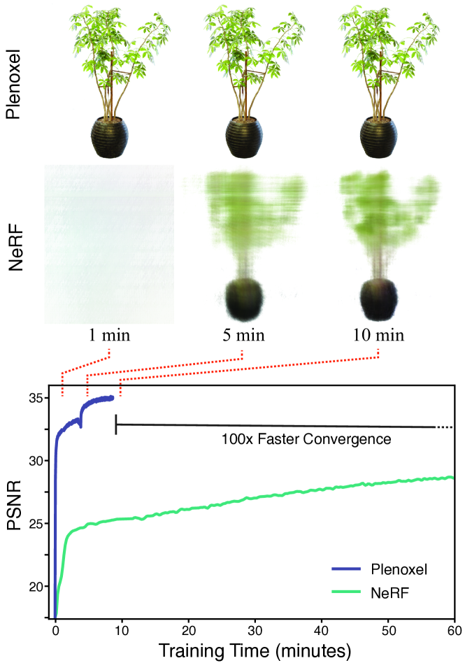
Figure 1: Plenoxel: Plenoptic Volume Elements for fast optimization of radiance fields. We show that direct optimization of a fully explicit 3D model can match the rendering quality of modern neural based approaches such as NeRF while optimizing over two orders of magnitude faster.

In this paper, we show that we can train a radiance field from scratch, without neural networks, while maintaining NeRF quality and reducing optimization time by two orders of magnitude. We provide a custom CUDA [29] implementation that capitalizes on the model simplicity to achieve substantial speedups. Our typical optimization time on a single Titan RTX GPU is 11 minutes on bounded scenes (compared to roughly 1 day for NeRF, more than a $100\times$ speedup) and 27 minutes on unbounded scenes (compared to roughly 4 days for NeRF++ [57], again more than a $100\times$ speedup). Although our implementation is not optimized for fast rendering, we can render novel viewpoints at interactive rates $15$ fps. If faster rendering is desired, our optimized Plenoxel model can be converted into a PlenOctree [56].

Specifically, we propose an explicit volumetric representation, based on a view-dependent sparse voxel grid without any neural networks. Our model can render photorealistic novel viewpoints and be optimized end-to-end from calibrated 2D photographs, using the differentiable rendering loss on training views as well as a total variation regularizer. We call our model Plenoxel for plenoptic volume elements, as it consists of a sparse voxel grid in which each voxel stores opacity and spherical harmonic coefficients. These coefficients are interpolated to model the full plenoptic function continuously in space. To achieve high resolution on a single GPU, we prune empty voxels and follow a coarse to fine optimization strategy. Although our core model is a bounded voxel grid, we can model unbounded scenes by using normalized device coordinates (for forward-facing scenes) or by surrounding our grid with multisphere images to encode the background (for $360^{\circ}$ scenes).

Our method reveals that photorealistic volumetric reconstruction can be approached using standard tools from inverse problems: a data representation, a forward model, a regularization function, and an optimizer. Our method shows that each of these components can be simple and state of the art results can still be achieved. Our experiments suggest the key element of Neural Radiance Fields is not the neural network but the differentiable volumetric renderer.

2 Related Work

Classical Volume Reconstruction.

We begin with a brief overview of classical methods for volume reconstruction, focusing on those which find application in our work. In particular, the most common classical methods for volume rendering are voxel grids [6, 42, 41, 13, 51, 43, 20] and multi-plane images (MPIs) [47, 32, 59, 46, 25, 55]. Voxel grids are capable of representing arbitrary topologies but can be memory limited at high resolution. One approach for reducing the memory requirement for voxel grids is to encode hierarchical structure, for instance using octrees [38, 11, 50, 52] (see [16] for a survey); we use an even simpler sparse array structure. Using these grid-based representations combined with some form of interpolation produces a continuous representation that can be arbitrarily resized using standard signal processing methods (see [30] for reference). This combination of sparsity and interpolation enables even a simple grid-based model to represent 3D scenes at high resolution without prohibitive memory requirements. We combine this classical sampling and interpolation paradigm with the forward volume rendering formula introduced by Max [22] (based on work from Kajiya and Von Herzen [12] and used in NeRF) to directly optimize a 3D model from indirect 2D observations. We further extend these classical approaches by modeling view dependence, which we accomplish by optimizing spherical harmonic coefficients for each color channel at each voxel. Spherical harmonics are a standard basis for functions over the sphere, and have been used previously to represent view dependence [34, 45, 3, 56].

Neural Volume Reconstruction.

Recently, dramatic improvements in neural volume reconstruction have renewed interest in this direction. Neural implicit representations were first used to model occupancy [24, 5, 21] and signed distance to an object’s surface [31, 48], and perform novel view synthesis from 3D point clouds [1, 40, 54, 17]. Several papers extended this idea of neural implicit 3D modeling to model a scene using only calibrated 2D image supervision via a differentiable volume rendering formulation [43, 44, 20, 26].

NeRF [26] in particular uses a differentiable volume rendering formula to train a coordinate-based multilayer perceptron (MLP) to directly predict color and opacity from 3D position and 2D viewing direction. NeRF produces impressive results but requires several days for full training, and about half an minute to render a full image, because every rendered pixel requires evaluating the coordinate-based MLP at hundreds of sample locations along the corresponding ray. Many papers have since extended the capabilities of NeRF, including modeling the background in $360^{\circ}$ views [57] and incorporating anti-aliasing for multiscale rendering [2]. We extend our Plenoxel method to unbounded $360^{\circ}$ scenes using a background model inspired by NeRF++ [57].

Of these methods, Neural Volumes [20] is the most similar to ours in that it uses a voxel grid with interpolation, but optimizes this grid through a convolutional neural network and applies a learned warping function to improve the effective resolution (of a $128^{3}$ grid). We show that the voxel grid can be optimized directly and high resolution can be achieved by pruning and coarse to fine optimization, without any neural networks or warping functions.

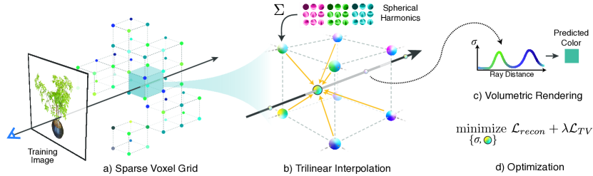
Figure 2: Overview of our sparse Plenoxel model. Given a set of images of an object or scene, we reconstruct a (a) sparse voxel (“Plenoxel”) grid with density and spherical harmonic coefficients at each voxel. To render a ray, we (b) compute the color and opacity of each sample point via trilinear interpolation of the neighboring voxel coefficients. We integrate the color and opacity of these samples using (c) differentiable volume rendering, following the recent success of NeRF [26]. The voxel coefficients can then be (d) optimized using the standard MSE reconstruction loss relative to the training images, along with a total variation regularizer.

Accelerating NeRF.

In light of the substantial computational requirements of NeRF for both training and rendering, many recent papers have proposed methods to improve efficiency, particularly for rendering. Among these methods are many that achieve speedup by subdividing the 3D volume into regions that can be processed more efficiently [35, 19]. Other speedup approaches have focused on a range of computational and pre- or post-processing methods to remove bottlenecks in the original NeRF formulation. JAXNeRF [7], a JAX [4] reimplementation of NeRF offers a speedup for both training and rendering via parallelization across many GPUs or TPUs. AutoInt [18] restructures the coordinate-based MLP to compute ray integrals exactly, for more than $10\times$ faster rendering with a small loss in quality. Learned Initializations [49] employs meta-learning on many scenes to start from a better MLP initialization, for both $>10\times$ faster training and better priors when per-scene data is limited. Other methods [27, 33, 14] achieve speedup by predicting a surface or sampling near the surface, reducing the number of samples necessary for rendering each ray.

Another approach is to pretrain a NeRF (or similar model) and then extract it into a different data structure that can support fast inference [8, 9, 36, 56]. In particular, PlenOctrees [56] extracts a NeRF variant into a sparse voxel grid in which each voxel represents view-dependent color using spherical harmonic coefficients. Because the extracted PlenOctree can be further optimized, this method can speed up training by roughly $3\times$, and because it uses an efficient GPU octree implementation without any MLP evaluations, it achieves $>3000\times$ rendering speedup. Our method extends PlenOctrees to perform end-to-end optimization of a sparse voxel representation with spherical harmonics, offering much faster training (two orders of magnitude speedup compared to NeRF). Our Plenoxel model is a generalization of PlenOctrees to support sparse plenoptic voxel grids of arbitrary resolution (not necessary powers of two) with the ability to perform trilinear interpolation, which is easier to implement with this sparse voxel structure.

3 Method

Our model is a sparse voxel grid in which each occupied voxel corner stores a scalar opacity $\sigma$ and a vector of spherical harmonic (SH) coefficients for each color channel. From here on we refer to this representation as Plenoxel. The opacity and color at an arbitrary position and viewing direction are determined by trilinearly interpolating the values stored at the neighboring voxels and evaluating the spherical harmonics at the appropriate viewing direction. Given a set of calibrated images, we optimize our model directly using the rendering loss on training rays. Our model is illustrated in Fig. 2 and described in detail below.

3.1 Volume Rendering

We use the same differentiable model for volume rendering as in NeRF, where the color of a ray is approximated by integrating over samples taken along the ray:

$$\hat{C}(\textbf{r})=\sum_{i=1}^{N}T_{i}\big{(}1-\exp(-\sigma_{i}\delta_{i})\big{)}\textbf{c}_{i}$$ (1)

$$\text{where }\hskip 20.00003ptT_{i}=\exp\left(-\sum_{j=1}^{i-1}\sigma_{j}\delta_{j}\right)$$ (2)

$T_{i}$ represents how much light is transmitted through ray r to sample $i$ (versus contributed by preceding samples), $\left(1-\exp(-\sigma_{i}\delta_{i})\right)$ denotes how much light is contributed by sample $i$, $\sigma_{i}$ denotes the opacity of sample $i$, and $\textbf{c}_{i}$ denotes the color of sample $i$, with distance $\delta_{i}$ to the next sample. Although this formula is not exact (it assumes single-scattering [12] and constant values between samples [22]), it is differentiable and enables updating the 3D model based on the error of each training ray.

3.2 Voxel Grid with Spherical Harmonics

Similar to PlenOctrees [56], we use a sparse voxel grid for our geometry model. However, for simplicity and ease of implementing trilinear interpolation, we do not use an octree for our data structure. Instead, we store a dense 3D index array with pointers into a separate data array containing values for occupied voxels only. Like PlenOctrees, each occupied voxel stores a scalar opacity $\sigma$ and a vector of spherical harmonic coefficients for each color channel. Spherical harmonics form an orthogonal basis for functions defined over the sphere, with low degree harmonics encoding smooth (more Lambertian) changes in color and higher degree harmonics encoding higher-frequency (more specular) effects. The color of a sample $\textbf{c}_{i}$ is simply the sum of these harmonic basis functions for each color channel, weighted by the corresponding optimized coefficients and evaluated at the appropriate viewing direction. We use spherical harmonics of degree 2, which requires 9 coefficients per color channel for a total of 27 harmonic coefficients per voxel. We use degree 2 harmonics because PlenOctrees found that higher order harmonics confer only minimal benefit.

Our Plenoxel grid uses trilinear interpolation to define a continuous plenoptic function throughout the volume. This is in contrast to PlenOctrees, which assumes that the opacity and spherical harmonic coefficients remain constant inside each voxel. This difference turns out to be an important factor in successfully optimizing the volume, as we discuss below. All coefficients (for opacity and spherical harmonics) are optimized directly, without any special initialization or pretraining with a neural network.

3.3 Interpolation

The opacity and color at each sample point along each ray are computed by trilinear interpolation of opacity and harmonic coefficients stored at the nearest 8 voxels. We find that trilinear interpolation significantly outperforms a simpler nearest neighbor interpolation; an ablation is presented in Tab. 1. The benefits of interpolation are twofold: interpolation increases the effective resolution by representing sub-voxel variations in color and opacity, and interpolation produces a continuous function approximation that is critical for successful optimization. Both of these effects are evident in Tab. 1: doubling the resolution of a nearest-neighbor-interpolating Plenoxel closes much of the gap between nearest neighbor and trilinear interpolation at a fixed resolution, yet some gap remains due to the difficulty of optimizing a discontinuous model. Indeed, we find that trilinear interpolation is more stable with respect to variations in learning rate compared to nearest neighbor interpolation (we tuned the learning rates separately for each interpolation method in Tab. 1, to provide close to the best number possible for each setup).

	PSNR $\uparrow$	SSIM $\uparrow$	LPIPS $\downarrow$
Trilinear, $256^{3}$	30.57	0.950	0.065
Trilinear, $128^{3}$	28.46	0.926	0.100
Nearest Neighbor, $256^{3}$	27.17	0.914	0.119
Nearest Neighbor, $128^{3}$	23.73	0.866	0.176

Table 1: Ablation over interpolation method. Results are averaged over the 8 NeRF synthetic scenes. We find that trilinear interpolation provides dual benefits of improving effective resolution and improving optimization, such that trilinear interpolation at resolution $128^{3}$ outperforms nearest neighbor interpolation at $256^{3}$.

3.4 Coarse to Fine

We achieve high resolution via a coarse-to-fine strategy that begins with a dense grid at lower resolution, optimizes, prunes unnecessary voxels, refines the remaining voxels by subdividing each in half in each dimension, and continues optimizing. For example, in the synthetic case, we begin with $256^{3}$ resolution and upsample to $512^{3}$. We use trilinear interpolation to initialize the grid values after each voxel subdivision step. In fact, we can resize between arbitrary resolutions using trilinear interpolation. Voxel pruning is performed using the method from PlenOctrees [56], which applies a threshold to the maximum weight $T_{i}(1-\exp(-\sigma_{i}\delta_{i}))$ of each voxel over all training rays (or, alternatively, to the density value in each voxel). Due to trilinear interpolation, naively pruning can adversely impact the the color and density near surfaces since values at these points interpolate with the voxels in the immediate exterior. To solve this issue, we perform a dilation operation so that a voxel is only pruned if both itself and its neighbors are deemed unoccupied.

3.5 Optimization

We optimize voxel opacities and spherical harmonic coefficients with respect to the mean squared error (MSE) over rendered pixel colors, with total variation (TV) regularization [39]. Specifically, our base loss function is:

$$\mathcal{L}=\mathcal{L}_{recon}+\lambda_{TV}\,\mathcal{L}_{TV}$$ (3)

Where the MSE reconstruction loss $\mathcal{L}_{recon}$ and the total variation regularizer $\mathcal{L}_{TV}$ are:

$$\mathcal{L}_{recon} =\frac{1}{|\mathcal{R}|}\sum_{\textbf{r}\in\mathcal{R}}\lVert C(\textbf{r})-\hat{C}(\textbf{r})\rVert_{2}^{2}$$

$$\mathcal{L}_{TV} =\frac{1}{|\mathcal{V}|}\sum_{\begin{subarray}{c}\mathbf{v}\in\mathcal{V}\\ d\in[D]\end{subarray}}\sqrt{\Delta_{x}^{2}(\mathbf{v},d)+\Delta_{y}^{2}(\mathbf{v},d)+\Delta_{z}^{2}(\mathbf{v},d)}$$

with $\Delta_{x}^{2}(\mathbf{v},d)$ shorthand for the squared difference between the $d$th value in voxel $\mathbf{v}:=(i,j,k)$ and the $d$th value in voxel $(i+1,j,k)$ normalized by the resolution, and analogously for $\Delta_{y}^{2}(\mathbf{v},d)$ and $\Delta_{z}^{2}(\mathbf{v},d)$. Note in practice we use different weights for SH coefficients and $\sigma$ values. These weights are fixed for each scene type (bounded, forward-facing, and $360^{\circ}$).

For faster iteration, we use a stochastic sample of the rays $\mathcal{R}$ to evaluate the MSE term and a stochastic sample of the voxels $\mathcal{V}$ to evaluate the TV term in each optimization step. We use the same learning rate schedule as JAXNeRF and Mip-NeRF [7, 2], but tune the initial learning rate separately for opacity and harmonic coefficients. The learning rate is fixed for all scenes in all datasets in the main experiments.

Directly optimizing voxel coefficients is a challenging problem for several reasons: there are many values to optimize (the problem is high-dimensional), the optimization objective is nonconvex due to the rendering formula, and the objective is poorly conditioned. Poor conditioning is typically best resolved by using a second order optimization algorithm (e.g. as recommended in [28]), but this is practically challenging to implement for a high-dimensional optimization problem because the Hessian is too large to easily compute and invert in each step. Instead, we use RMSProp [10] to ease the ill-conditioning problem without the full computational complexity of a second-order method.

3.6 Unbounded Scenes

We show that Plenoxels can be optimized for a wide range of settings beyond the synthetic scenes from the original NeRF paper.

With minor modifications, Plenoxels extend to real, unbounded scenes, both forward-facing and $360^{\circ}$. For forward-facing scenes, we use the same sparse voxel grid structure with normalized device coordinates, as defined in the original NeRF paper [26].

Background model.

For $360^{\circ}$ scenes, we augment our sparse voxel grid foreground representation with a multi-sphere image (MSI) background model, which also uses learned voxel colors and opacities with trilinear interpolation within and between spheres. Note that this is effectively the same as our foreground model, except the voxels are warped into spheres using the simple equirectangular projection (voxels index over sphere angles $\theta$ and $\phi$). We place 64 spheres linearly in inverse radius from $1$ to $\infty$ (we pre-scale the inner scene to be approximately contained in the unit sphere). To conserve memory, we store only rgb channels for the colors (only zero-order SH) and store all layers sparsely by using opacity thresholding as in our main model. This is similar to the background model in NeRF++ [57].

3.7 Regularization

We illustrate the importance of TV regularization in Fig. 3. In addition to TV regularization, which encourages smoothness and is used on all scenes, for certain types of scenes we also use additional regularizers.

(a) Full

(b) No SH TV

(c) No $\sigma$ TV

(d) No TV

Figure 3: Ablation over TV regularization. Clear artifacts are visible in the forward-facing scenes without TV on both $\sigma$ and SH coefficients, although PSNR does not always reflect this.

On the real, forward-facing and $360^{\circ}$ scenes, we use a sparsity prior based on a Cauchy loss following SNeRG [9]:

$$\mathcal{L}_{s}=\lambda_{s}\sum_{i,k}\log\left(1+2\sigma(\mathbf{r}_{i}(t_{k}))^{2}\right)$$ (4)

where $\sigma(\mathbf{r}_{i}(t_{k}))$ denotes the opacity of sample $k$ along training ray $i$. In each minibatch of optimization on forward-facing scenes, we evaluate this loss term at each sample on each active ray. This is also similar to the sparsity loss used in PlenOctrees [56] and encourages voxels to be empty, which helps to save memory and reduce quality loss when upsampling.

On the real, $360^{\circ}$ scenes, we also use a beta distribution regularizer on the accumulated foreground transmittance of each ray in each minibatch. This loss term, following Neural Volumes [20], promotes a clear foreground-background decomposition by encouraging the foreground to be either fully opaque or empty. This beta loss is:

$$\mathcal{L}_{\beta}=\lambda_{\beta}\sum_{\mathbf{r}}\left(\log(T_{FG}(\mathbf{r}))+\log(1-T_{FG}(\mathbf{r}))\right)$$ (5)

where $\mathbf{r}$ are the training rays and $T_{FG}(\mathbf{r})$ is the accumulated foreground transmittance (between 0 and 1) of ray $\mathbf{r}$.

3.8 Implementation

Since sparse voxel volume rendering is not well-supported in modern autodiff libraries, we created a custom PyTorch CUDA [29] extension library to achieve fast differentiable volume rendering; we hope practitioners will find this implementation useful in their applications. We also provide a slower, higher-level JAX [4] implementation. Both implementations will be released to the public.

The speed of our implementation is possible in large part because the gradient of our Plenoxel model becomes very sparse very quickly, as shown in Fig. 4. Within the first 1-2 minutes of optimization, fewer than 10% of the voxels have nonzero gradients.

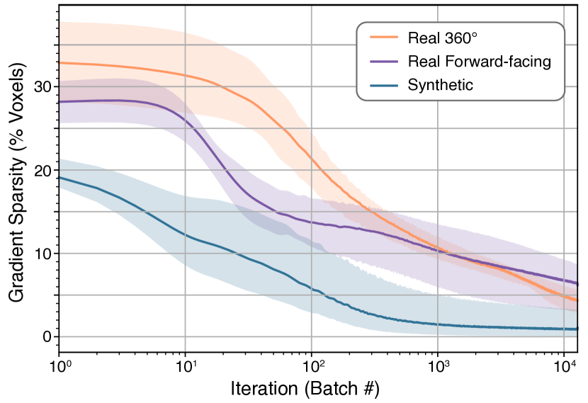
Figure 4: Gradient sparsity. The gradient becomes very sparse spatially within the first 12800 batches (one epoch for the synthetic scenes), with as few as 1% of the voxels updating per batch in the synthetic case. This enables efficient training via sparse parameter updates. The solid lines show the mean and the shaded regions show the full range of values among all scenes of each type.

4 Results

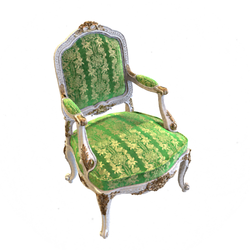
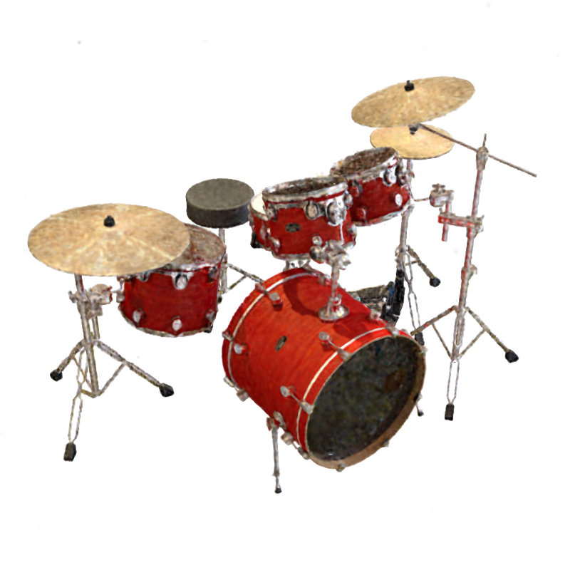
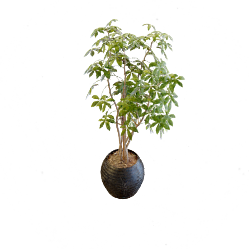
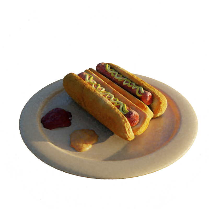
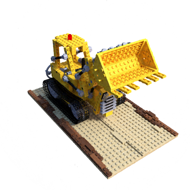
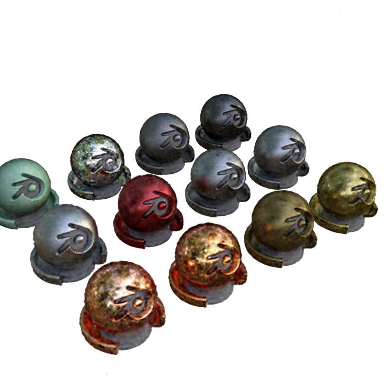
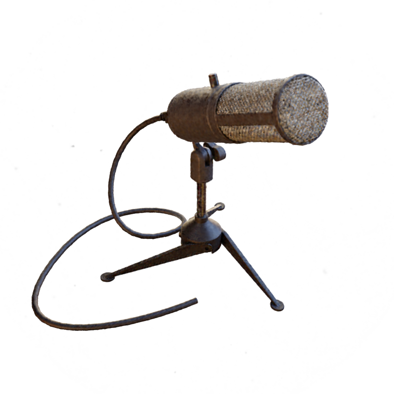
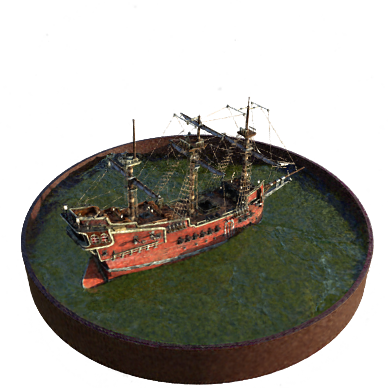
Figure 5: 1 minute, 20 seconds. Results on the synthetic scenes after 1 epoch of optimization, an average of 1 minute and 20 seconds.

We present results on synthetic, bounded scenes; real, unbounded, forward-facing scenes; and real, unbounded, $360^{\circ}$ scenes. We include time trial comparisons with prior work, showing dramatic speedup in training compared to all prior methods (alongside real-time rendering). Quantitative comparisons are presented in Tab. 2, and visual comparisons are shown in Fig. 6, Fig. 7, and Fig. 9. Our method achieves quality results after even the first epoch of optimization, less than 1.5 minutes, as shown in Fig. 5.

We also present the results from various ablation studies of our method. In the main text we present average results (PSNR, SSIM [53], and VGG LPIPS [58]) over all scenes of each type; full results on each scene individually are included in the supplement. We include full experimental details (hyperparameters, etc.) in the supplement.

4.1 Synthetic Scenes

Our synthetic experiments use the 8 scenes from NeRF: chair, drums, ficus, hotdog, lego, materials, mic, and ship. Each scene includes 100 ground truth training views with 800 $\times$ 800 resolution, from known camera positions distributed randomly in the upper hemisphere facing the object, which is set against a plain white background. Each scene is evaluated on 200 test views, also with resolution 800 $\times$ 800 and known inward-facing camera positions in the upper hemisphere. We provide quantitative comparisons in Tab. 2 and visual comparisons in Fig. 6.

	PSNR $\uparrow$	SSIM $\uparrow$	LPIPS $\downarrow$	Train Time
Ours	31.71	0.958	0.049	11 mins
NV [20]	26.05	0.893	0.160	$>$1 day
JAXNeRF [26, 7]	31.85	0.954	0.072	1.45 days
Ours	26.29	0.839	0.210	24 mins
LLFF [25]	24.13	0.798	0.212	—*
JAXNeRF [26, 7]	26.71	0.820	0.235	1.62 days
Ours	20.40	0.696	0.420	27 mins
NeRF++ [57]	20.49	0.648	0.478	$\sim$4 days

Table 2: Results. Top: average over the 8 synthetic scenes from NeRF; Middle: the 8 real, forward-facing scenes from NeRF; Bottom: the 4 real, $360^{\circ}$ scenes from Tanks and Temples [15]. 4 of the synthetic scenes train in under 10 minutes. *LLFF requires pretraining a network to predict MPIs for each view, and then can render novel scenes without further training; this pretraining is amortized across all scenes so we do not include it in the table.

(a) Ground Truth

(b) JAXNeRF [7, 26]

(c) Plenoxels

Figure 6: Synthetic, bounded scenes. Example results on the lego and ship synthetic scenes from NeRF [26]. Please see the supplementary material for more images.

We compare our method to Neural Volumes (NV) [20] (as a prior method that predicts a grid for each scene, using a 3D convolutional network), and JAXNeRF [26, 7]. For Neural Volumes we use values reported in [26]; for JAXNeRF we report results from our own rerunning, fixing the centered pixel bug. Our method achieves comparable quality compared to the best baseline, while training in an average of 11 minutes per scene on a single GPU and supporting interactive rendering.

4.2 Real Forward-Facing Scenes

We extend our method to unbounded, forward-facing scenes by using normalized device coordinates (NDC), as derived in NeRF [26]. Our method is otherwise identical to the version we use on bounded, synthetic scenes, except that we use TV regularization (with a stronger weight) throughout the optimization. This change is likely necessary because of the reduced number of training views for these scenes, as described in Sec. 4.4.

Our forward-facing experiments use the same 8 scenes as in NeRF, 5 of which are originally from LLFF [25]. Each scene consists of 20 to 60 forward-facing images captured by a handheld cell phone with resolution 1008 $\times$ 756, with $\frac{7}{8}$ of the images used for training and the remaining $\frac{1}{8}$ of the images reserved as a test set.

We compare our method to Local Light Field Fusion (LLFF) [25] (a prior method that uses a 3D convolutional network to predict a grid for each input view) and JAXNeRF. We provide quantitative comparisons in Tab. 2 and visual comparisons in Fig. 7.

(a) Ground Truth

(b) JAXNeRF [7, 26]

(c) Plenoxels

Figure 7: Real, forward-facing scenes. Example results on the fern and orchid forward-facing scenes from NeRF.

4.3 Real $360^{\circ}$ Scenes

We extend our method to real, unbounded, $360^{\circ}$ scenes by surrounding our sparse voxel grid with an multi-sphere image (MSI, based on multi-plane images introduced by [59]) background model, in which each background sphere is also a simple voxel grid with trilinear interpolation (both within each sphere and between adjacent background sphere layers).

Our $360^{\circ}$ experiments use 4 scenes from the Tanks and Temples dataset [15]: M60, playground, train, and truck. For each scene, we use the same train/test split as [37].

We compare our method to NeRF++ [57], which augments NeRF with a background model to represent unbounded scenes. We present quantitative comparisons in Tab. 2 and visual comparisons in Fig. 9.

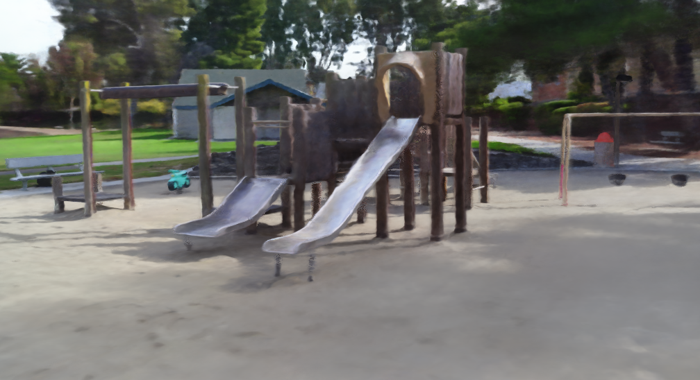
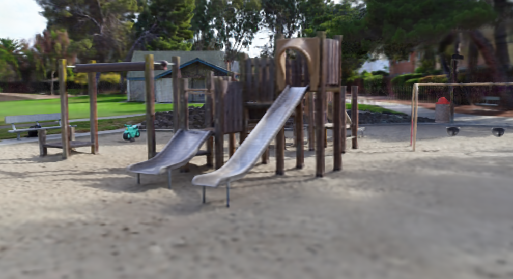
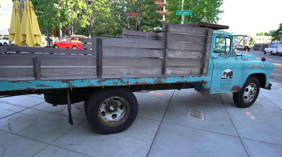
(a) Ground Truth

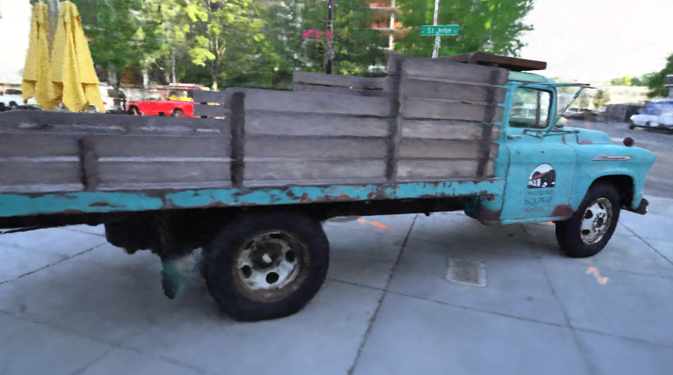
(b) NeRF++ [57]

(c) Plenoxels

Figure 9: Real, $360^{\circ}$ scenes. Example results on the playground and truck $360^{\circ}$ scenes from Tanks and Temples [15].

4.4 Ablation Studies

In this section, we perform extensive ablation studies of our method to understand which features are core to its success, with such a simple model. In Tab. 1, we show that continuous (in our case, trilinear) interpolation is responsible for dramatic improvement in fidelity compared to nearest neighbor interpolation (i.e. constant within each voxel) [56].

In Tab. 3, we consider how our method handles a dramatic reduction in training data, from 100 views to 25 views, on the 8 synthetic scenes. We compare our method to NeRF and find that, despite its lack of complex neural priors, by increasing TV regularization our method can outperform NeRF even in this limited data regime. This ablation also sheds light on why our model performs better with higher TV regularization on the real forward-facing scenes compared to the synthetic scenes: the real scenes have many fewer training images, and the stronger regularizer helps our optimization extend smoothly to sparsely-supervised regions.

We also ablate over the resolution of our Plenoxel grid in Tab. 4 and the rendering formula in Tab. 5. The rendering formula from Max [22] yields a substantial improvement compared to that of Neural Volumes [20], perhaps because it is more physically accurate (as discussed further in the supplement). The supplement also includes ablations over the learning rate schedule and optimizer demonstrating Plenoxel optimization to be robust to these hyperparameters.

	PSNR $\uparrow$	SSIM $\uparrow$	LPIPS $\downarrow$
Ours: 100 images (low TV)	31.71	0.958	0.050
NeRF: 100 images [26]	31.01	0.947	0.081
Ours: 25 images (low TV)	26.88	0.911	0.099
Ours: 25 images (high TV)	28.25	0.932	0.078
NeRF: 25 images [26]	27.78	0.925	0.108

Table 3: Ablation over the number of views. By increasing our TV regularization, we exceed NeRF fidelity even when the number of training views is only a quarter of the full dataset. Results are averaged over the 8 synthetic scenes from NeRF.

Resolution	PSNR $\uparrow$	SSIM $\uparrow$	LPIPS $\downarrow$
$512^{3}$	31.71	0.958	0.050
$256^{3}$	30.57	0.950	0.065
$128^{3}$	28.46	0.926	0.100
$64^{3}$	26.11	0.892	0.139
$32^{3}$	23.49	0.859	0.174

Table 4: Ablation over the Plenoxel grid resolution. Results are averaged over the 8 synthetic scenes from NeRF.

Rendering Formula	PSNR $\uparrow$	SSIM $\uparrow$	LPIPS $\downarrow$
Max [22], used in NeRF [26]	30.57	0.950	0.065
Neural Volumes [20]	27.54	0.906	0.201

Table 5: Comparison of different rendering formulas. We compare the rendering formula from Max [22] (used in NeRF and our main method) to the one used in Neural Volumes [20], which uses absolute instead of relative transmittance. Results are averaged over the 8 synthetic scenes from NeRF.

5 Discussion

We present a method for photorealistic scene modeling and novel viewpoint rendering that produces results with comparable fidelity to the state-of-the-art, while taking orders of magnitude less time to train. Our method is also strikingly straightforward, shedding light on the core elements that are necessary for solving 3D inverse problems: a differentiable forward model, a continuous representation (in our case, via trilinear interpolation), and appropriate regularization. We acknowledge that the ingredients for this method have been available for a long time, however nonlinear optimization with tens of millions of variables has only recently become accessible to the computer vision practitioner.

Limitations and Future Work.

As with any underdetermined inverse problem, our method is susceptible to artifacts. Our method exhibits different artifacts than neural methods, as shown in Fig. 10, but both methods achieve similar quality in terms of standard metrics (as presented in Sec. 4). Future work may be able to adjust or mitigate these remaining artifacts by studying different regularization priors and/or more physically accurate differentiable rendering functions.

Although we report all of our results for each dataset with a fixed set of hyperparameters, there is no optimal a priori setting of the TV weight $\lambda_{TV}$. In practice better results may be obtained by tuning this parameter on a scene-by-scene basis, which is possible due to our fast training time. This is expected because the scale, smoothness, and number of training views varies between scenes. We note that NeRF also has hyperparameters to be set such as the length of positional encoding, learning rate, and number of layers, and tuning these may also increase performance on a scene-by-scene basis.

(a) Ground Truth

(b) JAXNeRF [7, 26]

(c) Plenoxels

Figure 10: Artifacts. JAXNeRF and Plenoxel models both exhibit artifacts, but the artifacts are different, as shown here in the specularities in the synthetic drums scene. Note that some artifacts are unavoidable for any underdetermined inverse problem, but the specific artifacts vary depending on the priors induced by the model and regularizer.

Our method should extend naturally to support multiscale rendering with proper anti-aliasing through voxel cone-tracing, similar to the modifications in Mip-NeRF [2]. Another easy addition is tone-mapping to account for white balance and exposure changes, which we expect would help especially in the real $360^{\circ}$ scenes. A hierarchical data structure (such as an octree) may provide additional speedup compared to our sparse array implementation, provided that differentiable interpolation is preserved.

Since our method is two orders of magnitude faster than NeRF, we believe that it may enable downstream applications currently bottlenecked by the performance of NeRF–for example, multi-bounce lighting and 3D generative models across large databases of scenes. By combining our method with additional components such as camera optimization and large-scale voxel hashing, it may enable a practical pipeline for end-to-end photorealistic 3D reconstruction.

Plenoxels: Radiance Fields without Neural Networks
Supplementary Material

Appendix A Overview

In the supplementary material, we include additional experimental details and present results and visualizations of further ablation studies. We also present full, per-scene quantitative and visual comparisons between our method and prior work. We encourage the reader to see the video for results of our method on a wide range of scenes.

Appendix B Experimental Details

B.1 Implementation Details

As briefly discussed in Sec. 3.2, we use a simple data structure which consists of a data table in addition to a dense grid, where each cell is either NULL or a pointer into the data table. Each entry in the data table consists of the density value and the SH coefficients for each of the RGB color channels. NULL cells are considered to have all 0 values. This data structure allows for reasonably efficient trilinear interpolation both in the forward and backward passes while maintaining sparsity; due to the relatively large memory requirements to store the SH coefficients, gradients, and RMSProp running averages, the dense pointer grid is usually not dominant in size. Nevertheless, reading the pointers currently appears to take a significant amount of rendering time, and optimizations are likely possible.

Our main CUDA rendering and gradient kernels simultaneously parallelize across rays, colors, and SH coefficients. Each CUDA warp (32 threads) handles one ray, with threads processing one SH coefficient each; since coefficients are stored contiguously, this means access to global memory is highly coalesced. The SH coefficients are combined into colors using warp-level operations from NVIDIA CUB [23]. These features are particularly significant in the case of trilinear interpolation.

Note that in order to correctly perform trilinear color interpolation, instead of using the sigmoid function to ensure that predicted sample colors are always between 0 and 1 as in NeRF [26], we simply clip negative color values to 0 with a ReLU to preserve linearity as much as possible.

We use weight-based thresholding (as in PlenOctrees [56]) for the synthetic and real, $360^{\circ}$ scenes, and opacity-based thresholding for the forward-facing scenes. The reason for this is that some content (especially at the edges) in the forward-facing scenes is not visible in most of the training views, so weight-based thresholding tends to prune these sparsely-supervised features.

We use a batch size of 5000 rays and optimize with RMSProp [10]. For $\sigma$ we use the same delayed exponential learning rate schedule as Mip-NeRF [2], where the exponential is scaled by a learning rate of 30 (this is where the exponential would start, if not for the delay) and decays to 0.05 at step 250000, with an initial delay period of 15000 steps. For SH we use a pure exponential decay learning rate schedule, with an initial learning rate of 0.01 that decays to $5\text{\times}{10}^{-6}$ at step 250000.

The TV losses are evaluated stochastically; they are applied only to 1% of all voxels in the grid in each step. Note that empty voxels can be selected, as their neighbors may not be empty. In practice, for performance reasons, we always apply the TV regularization on random contiguous segments of voxels (in the order that the pointer grid is stored). This is much faster to evaluate on the GPU due to locality. In all cases, the voxel differences in the TV loss defined below Eq. 3 is in practice normalized by the voxel resolution in each dimension, relative to 256 (for historical reasons):

$$\Delta_{x}((i,j,k),d)=\frac{|V_{d}(i+1,j,k)-V_{d}(i,j,k)|}{256/D_{x}}$$ (6)

Where $D_{x}$ is the grid resolution in the $x$ dimension, and $V_{d}(i,j,k)$ is the $d$th value of voxel $(i,j,k)$ (either density or a SH coefficient). We scale $\Delta_{y},\Delta_{z}$ analogously. Note that the same loss is applied in NDC and to the background model, except in the background model, the TV also wraps around the edges of the equirectangular image. For SH, empty grid cells and edges are considered to have the same value as the current cell (instead of 0) for purposes of TV.

B.2 Synthetic experiments

On the synthetic scenes, we found that our method performs nearly identically when TV regularization is present only in the first stage of optimization; turning off the regularization after pruning voxels and increasing resolution reduces our training time modestly. We suspect (see Tab. 3) this is due to the large number of training views (100) available for these scenes as well as the low level of noise; for the other datasets we retain TV regularization throughout optimization.

We start at resolution $256^{3}$, prune and upsample to resolution $512^{3}$ after 38400 steps (the equivalent of 3 epochs), and optimize for a total of 128000 steps (the equivalent of 10 epochs). We prune using a weight threshold of 0.256, and use $\lambda_{TV}$ of $1\text{\times}{10}^{-5}$ for $\sigma$ and $1\text{\times}{10}^{-3}$ for SH, only during the initial 38400 steps (and then turn off regularization after pruning and upsampling, for faster optimization).

B.3 Forward-facing experiments

For the forward-facing scenes we start at resolution $256\times 256\times 128$, prune and upsample to resolution $512\times 512\times 128$ at step 38400, prune and upsample to resolution $1408\times 1156\times 128$ at step 76800, and optimize for a total of 128000 steps. The final grid resolution is derived from the image resolution of the dataset, with some padding added on each side. We prune using a $\sigma$ threshold of 5, use $\lambda_{TV}$ of $5\text{\times}{10}^{-4}$ for $\sigma$ and $5\text{\times}{10}^{-3}$ for SH, and use a sparsity penalty $\lambda_{s}$ of $1\text{\times}{10}^{-12}$ to encourage empty voxels.

While these TV parameters work well for the forward-facing NeRF scenes, more generally, we find that sometimes it is preferrable to use $\lambda_{TV}$ $5\text{\times}{10}^{-3}$ for density and $5\text{\times}{10}^{-2}$ for SH, which reduces artifacts while blurring the scene more. This is used for some of the examples in the video, for example the piano. In general, since scenes differ significantly in content, camera noise, and actual scale, a hyperparameter sweep of the TV weights can be helpful, and using different TV values across the scenes would improve the metrics for the NeRF scenes as well.

B.4 $360^{\circ}$ experiments

For the $360^{\circ}$ scenes our foreground Plenoxel grid starts at resolution $128^{3}$; we prune and upsample to $256^{3}$, $512^{3}$, and $640^{3}$ with 25600 steps in between each upsampling. We optimize for a total of 102400 steps. We prune using a weight threshold of 1.28, and use $\lambda_{TV}$ of $5\text{\times}{10}^{-5}$ for $\sigma$ and $5\text{\times}{10}^{-3}$ for SH for the inner grid and $\lambda_{TV}$ of $1\text{\times}{10}^{-3}$ for both $\sigma$ and SH for the 64 background grid layers of resolution $2048\times 1024$. We use $\lambda_{s}$ of $1\text{\times}{10}^{-11}$ and $\lambda_{\beta}$ of $1\text{\times}{10}^{-5}$. For simplicity of implementation, we did not use coarse-to-fine for the background and only use $\sigma$ thresholding. We also do not use the delayed learning rate function for the background, opting instead to use an exponential decay to allow the background to optimize faster than the foreground at the beginning.

While the TV weights were fixed for these scenes, in general, a hyperparameter sweep of the TV weights can be helpful. For more general scenes, it is sometimes useful to use a near-bound on the camera rays (as in NeRF) to prevent floaters very close to the camera, or to only begin optimizing the foreground after, say, 1000 iterations. Further sparsity losses to encourage the weight distribution to be a delta function may also help.

Appendix C Ablation Studies

We visualize ablations on the synthetic lego scene in Fig. 11. In addition to comparing nearest neighbor and trilinear interpolation, we also experimented with tricubic interpolation, which produces a function approximation that is both continuous (like trilinear interpolation) and smooth. However, we found tricubic interpolation offered negligible improvements compared to trilinear, in exchange for a substantial increase in computation (this increase in computation is why we do not include a full ablation table for tricubic interpolation).

(a) Trilinear, $256^{3}$

(b) Nearest, $256^{3}$

(c) Trilinear, $128^{3}$

(d) 25 Images, Low TV

(e) 25 Images, High TV

(f) NV Formula

Figure 11: Visual results of ablation studies on the synthetic lego scene. Trilinear interpolation at resolution $256^{3}$ is quite similar to our full model at resolution $512^{3}$. Nearest neighbor interpolation shows clear voxel artifacts. Trilinear interpolation at lower resolution appears less detailed. Reducing the number of training views produces visual artifacts that are mostly resolved by increasing the TV regularization. Optimizing and rendering with the Neural Volumes [20] formula produces different visual artifacts.

LR Schedule	PSNR $\uparrow$	SSIM $\uparrow$	LPIPS $\downarrow$
Exp for SH, Delayed for $\sigma$ [2]	30.57	0.950	0.065
Exp for SH and $\sigma$	30.58	0.950	0.066
Exp for SH, Constant for $\sigma$	30.37	0.948	0.068
Constant for SH and $\sigma$	30.13	0.945	0.075

Table 6: Comparison of different learning rate schedules for $\sigma$ (voxel opacity) and spherical harmonics (SH), with fixed resolution $256^{3}$ and RMSProp [10]. Results are averaged over the 8 synthetic scenes from NeRF [26]. Our method is robust to variations in learning rate schedule.

Optimizer	PSNR $\uparrow$	SSIM $\uparrow$	LPIPS $\downarrow$
RMSProp [10] for SH and $\sigma$	30.57	0.950	0.065
RMSProp for SH, SGD for $\sigma$	30.20	0.946	0.072
SGD for SH, RMSProp for $\sigma$	29.82	0.940	0.076
SGD for SH and $\sigma$	29.35	0.932	0.087

Table 7: Comparison of different optimizers for $\sigma$ and SH, with fixed resolution $256^{3}$. Results are averaged over the 8 synthetic scenes from NeRF [26]. Our method is robust to variations in optimizer, although there is a benefit to RMSProp particularly for optimizing the spherical harmonic coefficients.

Regularizer	PSNR $\uparrow$	SSIM $\uparrow$	LPIPS $\downarrow$
TV SH, TV $\sigma$, Sparsity	26.29	0.839	0.210
- Sparsity	26.31	0.839	0.210
- TV $\sigma$	25.25	0.807	0.226
- TV SH	25.80	0.814	0.234

Table 8: Ablation over regularization. Results are averaged over the 8 forward-facing scenes from NeRF, which are particularly sensitive to regularization due to the low number of training views. We find that the sparsity regularizer is not necessary for quality, but we retain it to reduce memory footprint. TV regularization is essential for $\sigma$ but also important for spherical harmonics, as visualized in Fig. 3, even though this effect is not as pronounced in the PSNR metric. Without any TV regularization (on SH or $\sigma$), three of the eight scenes run out of memory on our GPU.

Tab. 6 and Tab. 7 show ablations over learning rate schedule and optimizer, respectively. We find that Plenoxel optimization is reasonably robust to both of these hyperparameters, although there is a noticeable improvement from using RMSProp compared to SGD, particularly for the spherical harmonic coefficients. Note that when comparing different learning rate schedules and optimizers, we tune the initial learning rate separately for each row to provide the best results possible for each configuration.

Tab. 8 shows ablation over regularization, for the forward-facing scenes. We find that TV regularization is important for these scenes, likely due to their low number of training images. Regularization on opacity has a quantitatively larger effect than regularization on spherical harmonics, but both are important for avoiding visual artifacts (see Fig. 3).

Tab. 5 compares the performance of Plenoxels when trained with the rendering formula used in NeRF (originally from Max [22]) and when trained with the rendering formula used in Neural Volumes [20]. The Max formula is defined in Eq. 1 and rewritten here in a slightly more convenient format:

$$T_{i} =\exp\left(-\sum_{j=1}^{i-1}\sigma_{j}\delta_{j}\right)$$ (7)

$$\hat{C}(\textbf{r}) =\sum_{i=1}^{N}(T_{i}-T_{i+1})\textbf{c}_{i}$$ (8)

The Neural Volumes formula is (up to optimizing in log space):

$$T_{i} =\min\left\{1,~{}\sum_{j=1}^{i-1}\exp(-\delta_{i}\sigma_{i})\right\}$$ (9)

$$\hat{C}(\textbf{r}) =\sum_{i=1}^{N}(T_{i}-T_{i+1})\textbf{c}_{i}$$ (10)

These formulas only differ in their definition of the transmittance $T_{i}$. In particular, the Neural Volumes formula treats $\alpha_{i}$, the fraction of the ray contributed by sample $i$, as a function of the opacity and sampling distance of sample $i$ only. In contrast, the contribution of sample $i$ in the Max formula depends on the opacity of sample $i$ as well as the opacities of all preceding samples along the ray. In essence, opacity in the Neural Volumes formula is absolute and ray-independent (except for clipping the total contribution to 1), whereas opacity in the Max formula denotes the fraction of incoming light that each sample absorbs, a ray-dependent quantity. As we show in Tab. 5, the Max formula results in substantially better performance; we suspect this difference is due to its more physically-accurate modeling of transmittance.

Appendix D Per-Scene Results

D.1 Synthetic, Bounded Scenes

Full, per-scene results for the 8 synthetic scenes from NeRF are presented in Tab. 10 and Fig. 13. Note that the values for JAXNeRF are from our own rerunning with centered pixels (we ran JAXNeRF in parallel across 4 GPUs and multiplied the times by 4 to account for this parallelization).

D.2 Real, Forward-Facing Scenes

Full, per-scene results for the 8 forward-facing scenes from NeRF are presented in Tab. 11. Note that the values for JAXNeRF are from our own rerunning with centered pixels (we ran JAXNeRF in parallel across 4 GPUs and multiplied the times by 4 to account for this parallelization).

D.3 Real, $360^{\circ}$ Scenes

Full, per-scene results for the four $360^{\circ}$ scenes from Tanks and Temples [15] are presented in Tab. 9. Note that the values for NeRF++ appear slightly different from the paper; we re-evaluated the metrics independently using VGG LPIPS and standard SSIM, from rendered images shared by the original authors.

PSNR $\uparrow$
	M60	Playground	Train	Truck	Mean
Ours	17.93	23.03	17.97	22.67	20.40
NeRF++ [57]	18.49	22.93	17.77	22.77	20.49
SSIM $\uparrow$
	M60	Playground	Train	Truck	Mean
Ours	0.687	0.712	0.629	0.758	0.696
NeRF++	0.650	0.672	0.558	0.712	0.648
LPIPS $\downarrow$
	M60	Playground	Train	Truck	Mean
Ours	0.439	0.435	0.443	0.364	0.420
NeRF++	0.481	0.477	0.531	0.424	0.478
Optimization Time $\downarrow$
	M60	Playground	Train	Truck	Mean
Ours	25.5m	26.3m	29.5m	28.0m	27.3m

Table 9: Full results on $360^{\circ}$ scenes.

PSNR $\uparrow$
	Chair	Drums	Ficus	Hotdog	Lego	Materials	Mic	Ship	Mean
Ours	33.98	25.35	31.83	36.43	34.10	29.14	33.26	29.62	31.71
NV [20]	28.33	22.58	24.79	30.71	26.08	24.22	27.78	23.93	26.05
JAXNeRF [7, 26]	34.20	25.27	31.15	36.81	34.02	30.30	33.72	29.33	31.85
SSIM $\uparrow$
	Chair	Drums	Ficus	Hotdog	Lego	Materials	Mic	Ship	Mean
Ours	0.977	0.933	0.976	0.980	0.975	0.949	0.985	0.890	0.958
NV	0.916	0.873	0.910	0.944	0.880	0.888	0.946	0.784	0.893
JAXNeRF	0.975	0.929	0.970	0.978	0.970	0.955	0.983	0.868	0.954
LPIPS $\downarrow$
	Chair	Drums	Ficus	Hotdog	Lego	Materials	Mic	Ship	Mean
Ours	0.031	0.067	0.026	0.037	0.028	0.057	0.015	0.134	0.049
NV	0.109	0.214	0.162	0.109	0.175	0.130	0.107	0.276	0.160
JAXNeRF	0.036	0.085	0.037	0.074	0.068	0.057	0.023	0.192	0.072
Optimization Time $\downarrow$
	Chair	Drums	Ficus	Hotdog	Lego	Materials	Mic	Ship	Mean
Ours	9.6m	9.8m	8.8m	12.5m	10.8m	11.0m	8.2m	18.0m	11.1m
JAXNeRF	37.8h	37.8h	37.7h	38.0h	26.0h	38.1h	37.8h	26.0h	34.9h

Table 10: Full results on synthetic scenes.

(a) Ground Truth

(b) Neural Volumes

(c) JAXNeRF

(d) Plenoxels

Figure 12: Synthetic scenes. We show a random view from each of the synthetic scenes, comparing the ground truth, Neural Volumes [20], JAXNeRF [26, 7], and our Plenoxels.

(a) Ground Truth

(b) Neural Volumes

(c) JAXNeRF

(d) Plenoxels

Figure 13: Synthetic scenes. We show a random view from each of the synthetic scenes, comparing the ground truth, Neural Volumes [20], JAXNeRF [26, 7], and our Plenoxels.

PSNR $\uparrow$
	Fern	Flower	Fortress	Horns	Leaves	Orchids	Room	T-Rex	Mean
Ours	25.46	27.83	31.09	27.58	21.41	20.24	30.22	26.48	26.29
LLFF [25]	28.42	22.85	19.52	29.40	18.52	25.46	24.15	24.70	24.13
JAXNeRF [7, 26]	25.20	27.80	31.57	27.70	21.10	20.37	32.81	27.12	26.71
SSIM $\uparrow$
	Fern	Flower	Fortress	Horns	Leaves	Orchids	Room	T-Rex	Mean
Ours	0.832	0.862	0.885	0.857	0.760	0.687	0.937	0.890	0.839
LLFF	0.932	0.753	0.697	0.872	0.588	0.844	0.857	0.840	0.798
JAXNeRF	0.798	0.840	0.890	0.840	0.703	0.649	0.952	0.890	0.820
LPIPS $\downarrow$
	Fern	Flower	Fortress	Horns	Leaves	Orchids	Room	T-Rex	Mean
Ours	0.224	0.179	0.180	0.231	0.198	0.242	0.192	0.238	0.210
LLFF	0.155	0.247	0.216	0.173	0.313	0.174	0.222	0.193	0.212
JAXNeRF	0.272	0.198	0.151	0.249	0.305	0.307	0.164	0.235	0.235
Optimization Time $\downarrow$
	Fern	Flower	Fortress	Horns	Leaves	Orchids	Room	T-Rex	Mean
Ours	23.7m	22.0m	31.2m	26.3m	13.3m	23.4m	28.8m	24.8m	24.2m
JAXNeRF	38.9h	38.8h	38.6h	38.7h	38.8h	38.7h	39.1h	38.6h	38.8h

Table 11: Full results on forward-facing scenes.

(a) Ground Truth

(b) JAXNeRF

(c) Plenoxels

Figure 14: Forward-facing scenes. We show a random view from each of the forward-facing scenes, comparing the ground truth, JAXNeRF [26, 7], and our Plenoxels.

(a) Ground Truth

(b) JAXNeRF

(c) Plenoxels

Figure 15: Forward-facing scenes. We show a random view from each of the forward-facing scenes, comparing the ground truth, JAXNeRF [26, 7], and our Plenoxels. Note that these two methods have different behaviors in unsupervised regions (e.g. the bottom right in the orchids view): JAXNeRF fills in plausible textures whereas Plenoxels default to gray.

(a) Ground Truth

(b) NeRF++

(c) Plenoxels

Figure 16: $360^{\circ}$ scenes. We show a random view from each of the Tanks and Temples scenes, comparing the ground truth, NeRF++ [57], and our Plenoxels. We include two random views each for the M60 and train scenes, since the playground and truck scenes were shown in the main text.

References

- [1] Kara-Ali Aliev, Artem Sevastopolsky, Maria Kolos, Dmitry Ulyanov, and Victor Lempitsky. Neural point-based graphics. In Computer Vision–ECCV 2020: 16th European Conference, Glasgow, UK, August 23–28, 2020, Proceedings, Part XXII 16, pages 696–712. Springer, 2020.
- [2] Jonathan T. Barron, Ben Mildenhall, Matthew Tancik, Peter Hedman, Ricardo Martin-Brualla, and Pratul P. Srinivasan. Mip-NeRF: A multiscale representation for anti-aliasing neural radiance fields, 2021.
- [3] R. Basri and D.W. Jacobs. Lambertian reflectance and linear subspaces. IEEE Transactions on Pattern Analysis and Machine Intelligence, 25(2):218–233, 2003.
- [4] James Bradbury, Roy Frostig, Peter Hawkins, Matthew James Johnson, Chris Leary, Dougal Maclaurin, George Necula, Adam Paszke, Jake VanderPlas, Skye Wanderman-Milne, and Qiao Zhang. JAX: composable transformations of Python+NumPy programs, 2018.
- [5] Zhiqin Chen and Hao Zhang. Learning implicit fields for generative shape modeling, 2019.
- [6] Christopher B. Choy, Danfei Xu, JunYoung Gwak, Kevin Chen, and Silvio Savarese. 3d-r2n2: A unified approach for single and multi-view 3d object reconstruction, 2016.
- [7] Boyang Deng, Jonathan T. Barron, and Pratul P. Srinivasan. JaxNeRF: an efficient JAX implementation of NeRF, 2020.
- [8] Stephan J. Garbin, Marek Kowalski, Matthew Johnson, Jamie Shotton, and Julien Valentin. Fastnerf: High-fidelity neural rendering at 200fps, 2021.
- [9] Peter Hedman, Pratul P. Srinivasan, Ben Mildenhall, Jonathan T. Barron, and Paul Debevec. Baking neural radiance fields for real-time view synthesis, 2021.
- [10] Geoffrey Hinton. RMSProp.
- [11] Christian Häne, Shubham Tulsiani, and Jitendra Malik. Hierarchical surface prediction for 3d object reconstruction, 2017.
- [12] James T. Kajiya and Brian P Von Herzen. Ray tracing volume densities. In Proceedings of the 11th Annual Conference on Computer Graphics and Interactive Techniques, SIGGRAPH ’84, page 165–174, New York, NY, USA, 1984. Association for Computing Machinery.
- [13] Abhishek Kar, Christian Häne, and Jitendra Malik. Learning a multi-view stereo machine, 2017.
- [14] Petr Kellnhofer, Lars Jebe, Andrew Jones, Ryan Spicer, Kari Pulli, and Gordon Wetzstein. Neural lumigraph rendering, 2021.
- [15] Arno Knapitsch, Jaesik Park, Qian-Yi Zhou, and Vladlen Koltun. Tanks and temples: Benchmarking large-scale scene reconstruction. ACM Trans. Graph., 36(4), July 2017.
- [16] Aaron Knoll. A survey of octree volume rendering methods, 2006.
- [17] Christoph Lassner and Michael Zollhöfer. Pulsar: Efficient sphere-based neural rendering. In IEEE/CVF Conference on Computer Vision and Pattern Recognition (CVPR), June 2021.
- [18] David B. Lindell, Julien N. P. Martel, and Gordon Wetzstein. Autoint: Automatic integration for fast neural volume rendering, 2021.
- [19] Lingjie Liu, Jiatao Gu, Kyaw Zaw Lin, Tat-Seng Chua, and Christian Theobalt. Neural sparse voxel fields, 2021.
- [20] Stephen Lombardi, Tomas Simon, Jason Saragih, Gabriel Schwartz, Andreas Lehrmann, and Yaser Sheikh. Neural volumes. ACM Transactions on Graphics, 38(4):1–14, Jul 2019.
- [21] Julien N. P. Martel, David B. Lindell, Connor Z. Lin, Eric R. Chan, Marco Monteiro, and Gordon Wetzstein. Acorn: Adaptive coordinate networks for neural scene representation, 2021.
- [22] N. Max. Optical models for direct volume rendering. IEEE Transactions on Visualization and Computer Graphics, 1(2):99–108, 1995.
- [23] Duane Merrill and NVIDIA Corporation. CUB: Cooperative primitives for CUDA C++, 2021.
- [24] Lars Mescheder, Michael Oechsle, Michael Niemeyer, Sebastian Nowozin, and Andreas Geiger. Occupancy networks: Learning 3d reconstruction in function space, 2019.
- [25] Ben Mildenhall, Pratul P. Srinivasan, Rodrigo Ortiz-Cayon, Nima Khademi Kalantari, Ravi Ramamoorthi, Ren Ng, and Abhishek Kar. Local light field fusion: Practical view synthesis with prescriptive sampling guidelines, 2019.
- [26] Ben Mildenhall, Pratul P Srinivasan, Matthew Tancik, Jonathan T Barron, Ravi Ramamoorthi, and Ren Ng. Nerf: Representing scenes as neural radiance fields for view synthesis. In European conference on computer vision, pages 405–421. Springer, 2020.
- [27] T. Neff, P. Stadlbauer, M. Parger, A. Kurz, J. H. Mueller, C. R. A. Chaitanya, A. Kaplanyan, and M. Steinberger. Donerf: Towards real‐time rendering of compact neural radiance fields using depth oracle networks. Computer Graphics Forum, 40(4):45–59, Jul 2021.
- [28] Jorge Nocedal and Stephen J. Wright. Numerical Optimization. Springer, New York, NY, USA, second edition, 2006.
- [29] NVIDIA, Péter Vingelmann, and Frank H.P. Fitzek. Cuda, release: 10.2.89, 2020.
- [30] Alan V. Oppenheim and Ronald W. Schafer. Discrete-Time Signal Processing. Prentice Hall Press, USA, 3rd edition, 2009.
- [31] Jeong Joon Park, Peter Florence, Julian Straub, Richard Newcombe, and Steven Lovegrove. DeepSDF: Learning continuous signed distance functions for shape representation, 2019.
- [32] Eric Penner and Li Zhang. Soft 3d reconstruction for view synthesis. ACM Transactions on Graphics (TOG), 36:1 – 11, 2017.
- [33] Martin Piala and Ronald Clark. Terminerf: Ray termination prediction for efficient neural rendering, 2021.
- [34] Ravi Ramamoorthi and Pat Hanrahan. On the relationship between radiance and irradiance: determining the illumination from images of a convex lambertian object. JOSA A, 18(10):2448–2459, 2001.
- [35] Daniel Rebain, Wei Jiang, Soroosh Yazdani, Ke Li, Kwang Moo Yi, and Andrea Tagliasacchi. Derf: Decomposed radiance fields, 2020.
- [36] Christian Reiser, Songyou Peng, Yiyi Liao, and Andreas Geiger. KiloNeRF: Speeding up neural radiance fields with thousands of tiny mlps, 2021.
- [37] Gernot Riegler and Vladlen Koltun. Free view synthesis, 2020.
- [38] Gernot Riegler, Ali Osman Ulusoy, and Andreas Geiger. Octnet: Learning deep 3d representations at high resolutions, 2017.
- [39] Leonid I Rudin and Stanley Osher. Total variation based image restoration with free local constraints. In Proceedings of 1st International Conference on Image Processing, volume 1, pages 31–35. IEEE, 1994.
- [40] Darius Rückert, Linus Franke, and Marc Stamminger. Adop: Approximate differentiable one-pixel point rendering, 2021.
- [41] Seitz, Steven, Kutulakos, and Kiriakos. A theory of shape by space carving. 01 2000.
- [42] S.M. Seitz and C.R. Dyer. Photorealistic scene reconstruction by voxel coloring. In Proceedings of IEEE Computer Society Conference on Computer Vision and Pattern Recognition, pages 1067–1073, 1997.
- [43] Vincent Sitzmann, Justus Thies, Felix Heide, Matthias Nießner, Gordon Wetzstein, and Michael Zollhöfer. Deepvoxels: Learning persistent 3d feature embeddings, 2019.
- [44] Vincent Sitzmann, Michael Zollhöfer, and Gordon Wetzstein. Scene representation networks: Continuous 3d-structure-aware neural scene representations, 2020.
- [45] Peter-Pike Sloan, Jan Kautz, and John Snyder. Precomputed radiance transfer for real-time rendering in dynamic, low-frequency lighting environments. ACM Trans. Graph., 21(3):527–536, July 2002.
- [46] Pratul P. Srinivasan, Richard Tucker, Jonathan T. Barron, Ravi Ramamoorthi, Ren Ng, and Noah Snavely. Pushing the boundaries of view extrapolation with multiplane images, 2019.
- [47] Richard Szeliski and Polina Golland. Stereo matching with transparency and matting. International Journal of Computer Vision, 32:45–61, 2004.
- [48] Towaki Takikawa, Joey Litalien, Kangxue Yin, Karsten Kreis, Charles Loop, Derek Nowrouzezahrai, Alec Jacobson, Morgan McGuire, and Sanja Fidler. Neural geometric level of detail: Real-time rendering with implicit 3d shapes, 2021.
- [49] Matthew Tancik, Ben Mildenhall, Terrance Wang, Divi Schmidt, Pratul P. Srinivasan, Jonathan T. Barron, and Ren Ng. Learned initializations for optimizing coordinate-based neural representations, 2021.
- [50] Maxim Tatarchenko, Alexey Dosovitskiy, and Thomas Brox. Octree generating networks: Efficient convolutional architectures for high-resolution 3d outputs, 2017.
- [51] Shubham Tulsiani, Tinghui Zhou, Alexei A. Efros, and Jitendra Malik. Multi-view supervision for single-view reconstruction via differentiable ray consistency, 2017.
- [52] Peng-Shuai Wang, Yang Liu, Yu-Xiao Guo, Chun-Yu Sun, and Xin Tong. O-cnn. ACM Transactions on Graphics, 36(4):1–11, Jul 2017.
- [53] Zhou Wang, A.C. Bovik, H.R. Sheikh, and E.P. Simoncelli. Image quality assessment: from error visibility to structural similarity. IEEE Transactions on Image Processing, 13(4):600–612, 2004.
- [54] Olivia Wiles, Georgia Gkioxari, Richard Szeliski, and Justin Johnson. Synsin: End-to-end view synthesis from a single image, 2020.
- [55] Suttisak Wizadwongsa, Pakkapon Phongthawee, Jiraphon Yenphraphai, and Supasorn Suwajanakorn. Nex: Real-time view synthesis with neural basis expansion, 2021.
- [56] Alex Yu, Ruilong Li, Matthew Tancik, Hao Li, Ren Ng, and Angjoo Kanazawa. Plenoctrees for real-time rendering of neural radiance fields, 2021.
- [57] Kai Zhang, Gernot Riegler, Noah Snavely, and Vladlen Koltun. NeRF++: Analyzing and improving neural radiance fields, 2020.
- [58] Richard Zhang, Phillip Isola, Alexei A Efros, Eli Shechtman, and Oliver Wang. The unreasonable effectiveness of deep features as a perceptual metric. In CVPR, 2018.
- [59] Tinghui Zhou, Richard Tucker, John Flynn, Graham Fyffe, and Noah Snavely. Stereo magnification: Learning view synthesis using multiplane images, 2018.