Fair Community Detection and Structure Learning in Heterogeneous Graphical Models

Abstract

Inference of community structure in probabilistic graphical models may not be consistent with fairness constraints when nodes have demographic attributes. Certain demographics may be over-represented in some detected communities and under-represented in others. This paper defines a novel $\ell_{1}$-regularized pseudo-likelihood approach for fair graphical model selection. In particular, we assume there is some community or clustering structure in the true underlying graph, and we seek to learn a sparse undirected graph and its communities from the data such that demographic groups are fairly represented within the communities. In the case when the graph is known a priori, we provide a convex semidefinite programming approach for fair community detection. We establish the statistical consistency of the proposed method for both a Gaussian graphical model and an Ising model for, respectively, continuous and binary data, proving that our method can recover the graphs and their fair communities with high probability.

2010.00000

, and

1 Introduction

Probabilistic graphical models have been applied in a wide range of machine learning problems to infer dependency relationships among random variables. Examples include gene expression [85, 106], social interaction networks [98, 101], computer vision [52, 65, 73], and recommender systems [61, 104]. Since in most applications the number of model parameters to be estimated far exceeds the available sample size, it is necessary to impose structure, such as sparsity or community structure, on the estimated parameters to make the problem well-posed. With the increasing application of structured graphical models and community detection algorithms in human-centric contexts [99, 96, 42, 16, 87, 32], there is a growing concern that, if left unchecked, they can lead to discriminatory outcomes for protected groups. For instance, the proportion of a minority group assigned to some community can be far from its underlying proportion, even if detection algorithms do not take the minority sensitive attribute into account in decision making [29]. Such an outcome may, in turn, lead to unfair treatment of minority groups. For example, in precision medicine, patient-patient similarity networks over a biomarker feature space can be used to cluster a cohort of patients and support treatment decisions on particular clusters [84, 66]. If the clusters learned by the algorithm are demographically imbalanced, this treatment assignment may unfairly exclude under-represented groups from effective treatments.

To the best of our knowledge, the estimation of fair structured graphical models has not previously been addressed. However, there is a vast body of literature on learning structured probabilistic graphical models. Typical approaches to impose structure in graphical models, such as $\ell_{1}$-regularization, encourage sparsity structure that is uniform throughout the network and may therefore not be the most suitable choice for many real world applications where data have clusters or communities, i.e., groups of graph nodes with similar connectivity patterns or stronger connections within the group than to the rest of the network. Graphical models with these properties are called heterogeneous.

It is known that if the goal is structured heterogeneous graph learning, structure or community inference and graph weight estimation should be done jointly. In fact, performing structure inference before weight estimation results in a sub-optimal procedure [74]. To overcome this issue, some of the initial work focused on either inferring connectivity information or performing graph estimation in case the connectivity or community information is known a priori [31, 48, 40, 72, 68]. Recent developments consider the two tasks jointly and estimate the structured graphical models arising from heterogeneous observations [64, 54, 50, 101, 63, 41, 88, 21, 35].

In this paper, we develop a provably convergent penalized pseudo-likelihood method to induce fairness into clustered probabilistic graphical models. Our contributions are as follows:

• Fair Structure Learning in Graphical Models: We formulate a novel version of probabilistic graphical modeling that incorporates fairness considerations. We assume an underlying community structure in our graph and aim to learn an undirected graph from the data such that demographic groups are fairly represented within the communities.

• Fair Convex Community Detection: We provide a semidefinite programming for detecting fair communities within a known graph. This approach retains the computational complexity of convex community detection methods [8, 17, 70] while enhancing fairness in community structure.

• Unified Consistency Estimation Analysis: Our rigorous analysis shows high-probability recovery of fair communities within an unknown graph. We show that community estimators are asymptotically consistent in high-dimensional settings for Gaussian and Ising graphical models, assuming standard regularity conditions.

• We present numerical results from both synthetic and real-world datasets, highlighting the importance of proportional clustering. Comparisons of our method with traditional graphical models show our algorithms’ superior efficacy in estimating graphs and their communities, thus attaining higher fairness levels.

The remainder of the paper is organized as follows: Section 2 gives a general framework for fair structure learning in graphs. Section 3 gives a detailed statement of the proposed fair graphical models for continuous and binary datasets. In Sections 4 and 5, we illustrate the proposed framework on a number of synthetic and real data sets, respectively. Section 6 provides some concluding remarks.

Notation.

For a set $\mathcal{S}$, $|\mathcal{S}|$ is the cardinality of $\mathcal{S}$, and $\mathcal{S}^{c}$ is its complement. The reals and nonnegative reals fields are denoted as ${\mathbb{R}}$ and ${\mathbb{R}}_{+}$, respectively. We use lower-case and upper-case bold letters such as ${\bf{x}}$ and ${\bf{X}}$ to represent vectors and matrices, respectively, with $x_{i}$ and $x_{ij}$ denoting their elements. If all coordinates of a vector ${\bf{x}}$ are nonnegative, we write ${\bf{x}}\geq 0$. The notation ${\bf{x}}>0$, as well as ${\bf{X}}\geq 0$ and ${\bf{X}}>0$ for matrices, are defined similarly. For a symmetric matrix ${\bf{X}}\in{\mathbb{R}}^{n\times n}$, we write ${\bf{X}}\succ 0$ if ${\bf{X}}$ is positive definite, and ${\bf{X}}\succeq 0$ if it is positive semidefinite. ${\bf{I}}_{p}$, ${\bf{J}}_{p}$, and ${\bf{0}}_{p}$ denote the $p\times p$ identity matrix, matrix of all ones, and matrix of all zeros, respectively. We use $\Lambda_{i}({\bf{X}})$, $\Lambda_{\max}({\bf{X}})$ and $\Lambda_{\min}({\bf{X}})$ to denote the $i$-th, maximum, and minimum singular values of ${\bf{X}}$, respectively. For any matrix ${\bf{X}}$, we define $\|{\bf{X}}\|_{\infty}:=\max_{ij}|x_{ij}|$, $\|{\bf{X}}\|_{1}:=\sum_{ij}|x_{ij}|$, $\|{\bf{X}}\|:=\Lambda_{\max}({\bf{X}})$, and $\|{\bf{X}}\|_{\text{F}}:=\sqrt{\sum_{ij}|x_{ij}|^{2}}$.

2 Fair Structure Learning in Graphical Models

We introduce a fair graph learning method that simultaneously accounts for fair community detection and estimation of heterogeneous graphical models.

Let ${\bf{Y}}$ be an $n\times p$ matrix, with columns ${\bf{y}}_{1},\ldots,{\bf{y}}_{p}$. We associate to each column in ${\bf{Y}}$ a node in a graph $\mathcal{G}=(\mathcal{V},\mathcal{E})$, where $\mathcal{V}=\{1,2,\ldots,p\}$ is the vertex set and $\mathcal{E}\in\mathcal{V}\times\mathcal{V}$ is the edge set. We consider a simple undirected graph, without self-loops, and whose edge set contains only distinct pairs. Graphs are conveniently represented by a $p\times p$ matrix, denoted by $\Theta$, whose nonzero entries correspond to edges in the graph. The precise definition of this usually depends on modeling assumptions, properties of the desired graph, and application domain.

In order to obtain a sparse and interpretable graph estimate, many authors have considered the problem

$$~{}\begin{array}[]{ll}\underset{\mbox{\boldmath$\Theta$}}{\text{minimize}}&\begin{array}[]{c}\hskip 5.69046ptL(\mbox{\boldmath$\Theta$};{\bf{Y}})+\rho_{1}\|\mbox{\boldmath$\Theta$}\|_{1,\textnormal{off}}\end{array}\\ \text{subj. to}&\begin{array}[t]{l}\hskip 5.69046pt\mbox{\boldmath$\Theta$}\in\mathcal{M}.\end{array}\end{array}$$ (5)

Here, $L$ is a loss function; $\rho_{1}\|\mbox{\boldmath$\Theta$}\|_{1,\textnormal{off}}$ is the $\ell_{1}$-norm regularization applied to off-diagonal elements of $\Theta$ with parameter $\rho_{1}>0$; and $\mathcal{M}$ is a convex constraint subset of ${\mathbb{R}}^{p\times p}$. For instance, in the case of a Gaussian graphical model, we could take $L(\mbox{\boldmath$\Theta$};{\bf{Y}})=-\log\det(\mbox{\boldmath$\Theta$})+\operatorname{trace}({\bf{S}}\mbox{\boldmath$\Theta$})$, where ${\bf{S}}=n^{-1}\sum_{i=1}^{n}{\bf{y}}_{i}{\bf{y}}_{i}^{\top}$ and $\mathcal{M}$ is the set of $p\times p$ positive definite matrices. The solution to (5) can then be interpreted as a sparse estimate of the inverse covariance matrix [10, 38]. Throughout, we assume that $L(\mbox{\boldmath$\Theta$};{\bf{Y}})$ and $\mathcal{M}$ are convex function and set, respectively.

2.1 Model Framework

We build our fair graph learning framework using (5) as a starting point. Let $\mathcal{V}$ denote the set of nodes. Suppose there exist $K$ disjoint communities of nodes denoted by $\mathcal{V}=\mathcal{C}_{1}\cup\cdots\cup\mathcal{C}_{K}$ where $\mathcal{C}_{k}$ is the subset of nodes from $\mathcal{G}$ that belongs to the $k$–th community. For each candidate partition of $n$ nodes into $K$ communities, we associate it with a partition matrix ${\bf{Q}}\in[0,1]^{p\times p}$, such that $q_{ij}=1/|C_{k}|$ if and only if nodes $i$ and $j$ are assigned to the $k$th community. Let $\mathcal{Q}_{pK}$ be the set of all such partition matrices, and $\bar{{\bf{Q}}}$ the true partition matrix associated with the ground-truth clusters $\{\bar{\mathcal{C}}_{k}\}_{k=1}^{K}$.

Figure 1: Examples of probabilistic graphical models with $p=10$ nodes, and demographic groups $\mathcal{V}=\mathcal{D}_{1}\cup\mathcal{D}_{2}$, where $\mathcal{D}_{1}$ is the set of red nodes while $\mathcal{D}_{2}$ is the set of blue nodes. The left and right figures show the precision matrices associated with ${\bf{Q}}^{\prime}$ and ${\bf{Q}}$ (fair membership matrix) defined in Example 8, respectively. For the fair graphical model (right) with disjoin communities $\mathcal{C}_{1}$, $\mathcal{C}_{2}$, and $\mathcal{C}_{3}$, we have $|\mathcal{D}_{h}\cap\mathcal{C}_{k}|/|\mathcal{C}_{k}|=1/2=|\mathcal{D}_{h}|/p~{}~{}\textnormal{for all}~{}~{}k\in\{1,2,3\}$.

Assume the set of nodes contains $H$ demographic groups such that $\mathcal{V}=\mathcal{D}_{1}\cup\cdots\cup\mathcal{D}_{H}$, potentially with overlap between the groups. [29] proposed a model for fair clustering requiring the representation in each cluster to preserve the global fraction of each demographic group $\mathcal{D}_{h}$, i.e.,

$$\frac{|\mathcal{D}_{h}\cap\mathcal{C}_{k}|}{|\mathcal{C}_{k}|}=\frac{|\mathcal{D}_{h}|}{p}~{}~{}\textnormal{for all}~{}~{}k\in[K].$$ (6)

Let ${\bf{R}}\in\{0,1\}^{p\times p}$ be such that $r_{ij}=1$ if and only if nodes $i$ and $j$ are assigned to the same demographic group, with the convention that $r_{ii}=1,\forall i$. One will notice that (6) is equivalent to ${\bf{R}}({\bf{I}}-{\bf{J}}_{p}/p){\bf{Q}}=0$; see Figure 1 for an illustration.

Let ${\bf{A}}_{1}:={\bf{R}}({\bf{I}}-{\bf{J}}_{p}/p)$ and ${\bf{B}}_{1}:=\text{diag}(\mbox{\boldmath$\epsilon$}){\bf{J}}_{p}$ for some $\mbox{\boldmath$\epsilon$}>0$ that controls how close we are to exact demographic parity. Under this setting, we introduce a general optimization framework for fair structured graph learning via a trace regularization and a fairness constraint on the partition matrix ${\bf{Q}}$ as follows:

$$\begin{array}[]{ll}\underset{\mbox{\boldmath$\Theta$},~{}\mbox{\boldmath$Q$}}{\text{minimize}}&\begin{array}[]{c}\hskip 14.22636ptL(\mbox{\boldmath$\Theta$};{\bf{Y}})+\rho_{1}\|\mbox{\boldmath$\Theta$}\|_{1,\textnormal{off}}+\rho_{2}\operatorname{trace}\big{(}{\bf{Q}}G(\mbox{\boldmath$\Theta$})\big{)}\end{array}\\ \text{subj. to}&\begin{array}[t]{l}\hskip 5.69046pt\mbox{\boldmath$\Theta$}\in\mathcal{M},~{}~{}{\bf{A}}_{1}{\bf{Q}}\leq{\bf{B}}_{1},~{}~{}\text{and}~{}~{}{\bf{Q}}\in\cup_{K}\mathcal{Q}_{pK}.\end{array}\end{array}$$ (11)

Here, $G(\mbox{\boldmath$\Theta$}):\mathcal{M}\rightarrow\mathcal{M}$ is a function of $\Theta$ (introduced in Sections 3.1 and 3.2).

In Problem (11), the term $\rho_{1}\|\mbox{\boldmath$\Theta$}\|_{1,\textnormal{off}}$ shrinks small entries of $\Theta$ to $0$, thus enforcing sparsity in $\Theta$ and consequently in $\mathcal{G}$. This term controls the presence of edges between any two nodes irrespective of the community they belong to, with higher values for $\rho_{1}$ forcing sparser estimators. The polyhedral constraint is the fairness constraint, enforcing that every community contains the $\epsilon$-approximate proportion of elements from each demographic group $\mathcal{D}_{h}$, $h\in[H]$, matching the overall proportion. The term $\rho_{2}\operatorname{trace}\left({\bf{Q}}G(\mbox{\boldmath$\Theta$})\right)$ enforces community structure in a similarity graph, $G(\mbox{\boldmath$\Theta$})$. It should be mentioned that such trace regularization has been previously used in different forms [17, 8, 54, 88, 35] when estimating communities of networks. The intuition/interpretation behind the specific choice of the function $G({\Theta})$ is to connect the trace term and the loss function $L(\mbox{\boldmath$\Theta$};{\bf{Y}})$ in the different graphical models; see discussions in Sections 3 and 3.2.

The problem (11) is in general NP-hard due to its constraint on ${\bf{Q}}$. However, it can be relaxed to a computationally feasible problem. To do so, we exploit algebraic properties of a community matrix ${\bf{Q}}$. By definition, we see that ${\bf{Q}}$ must have the form ${\bf{Q}}=\mbox{\boldmath$\Psi$}\mbox{\boldmath$\Gamma$}\mbox{\boldmath$\Psi$}^{\intercal}$, where $\Gamma$ is block diagonal with size ${p_{k}}\times{p_{k}}$ blocks on the diagonal with blue all entries equal to $1/|C_{k}|$ associated with $k$-th community, $\Psi$ is some permutation matrix, and the number of communities $K$ is unknown. The set of all matrices ${{\bf{Q}}}$ of this form is non-convex. The key observation is that any such ${\bf{Q}}$ satisfies several convex constraints such as (i) all entries of ${\bf{Q}}$ are nonnegative, (ii) all diagonal entries of ${\bf{Q}}$ are $1/|C_{k}|$, and (iii) ${\bf{Q}}$ is positive semi-definite [17, 8, 70]. Without loss of generality, we assume that the permutation matrix corresponding to the ground truth communities is the identity, i.e., $\mbox{\boldmath$\Psi$}={\bf{I}}$. Now, let

$${\bf{A}}:=[{\bf{A}}_{1};{\bf{I}}_{p}],~{}~{}~{}\text{and}~{}~{}{\bf{B}}:=[{\bf{B}}_{1};{\bf{J}}_{p}].$$

Thus, we propose the following relaxation:

$$~{}\begin{array}[]{ll}\underset{\mbox{\boldmath$\Theta$},~{}{\bf{\mbox{\boldmath$Q$}}}}{\text{minimize}}&\begin{array}[]{c}\hskip 14.22636ptL(\mbox{\boldmath$\Theta$};{\bf{Y}})+\rho_{1}\|\mbox{\boldmath$\Theta$}\|_{1,\textnormal{off}}+\rho_{2}\operatorname{trace}\big{(}{\bf{Q}}G(\mbox{\boldmath$\Theta$})\big{)}\end{array}\\ \text{subj. to}&\begin{array}[t]{l}\hskip 14.22636pt\mbox{\boldmath$\Theta$}\in\mathcal{M},~{}~{}\textnormal{and}~{}~{}{\bf{Q}}\in\mathcal{N},\end{array}\end{array}$$ (12e)

where

$$\mathcal{N} =\left\{{\bf{Q}}\in{\mathbb{R}}^{p\times p}:~{}{\bf{Q}}\succeq{\bf{0}},~{}{\bf{0}}\leq{\bf{A}}{\bf{Q}}\leq{\bf{B}},~{}q_{ii}=1~{}\textnormal{for}~{}1\leq i\leq p\right\}.$$ (12f)

The solution of (12) jointly learns the fair community matrix ${\bf{Q}}$ and the network estimate $\Theta$. We highlight the following attractive properties of the formulation (12): (i) the communities are allowed to have significantly different sizes; (ii) the number of communities $K$ may grow as $p$ increases; (iii) the knowledge of $K$ is not required for fair community detection, and (iv) the objective function (12e) is convex in $\Theta$ given ${\bf{Q}}$ and conversely.

2.2 Algorithm

In order to solve (12), we use an alternating direction method of multipliers (ADMM) algorithm [15]. ADMM is an attractive algorithm for this problem, as it allows us to decouple some of the terms in (12) that are difficult to optimize jointly. In order to develop an ADMM algorithm for (12) with guaranteed convergence, we reformulate it as follows:

$$\operatorname*{minimize}_{\mbox{\boldmath$Q$},\mbox{\boldmath$\Theta$},\mbox{\boldmath$\Omega$}}~{}~{}~{}~{} L(\mbox{\boldmath$\Theta$};{\bf{Y}})+\rho_{1}\|\mbox{\boldmath$\Omega$}\|_{1,\textnormal{off}}+\rho_{2}\operatorname{trace}\big{(}{\bf{Q}}G(\mbox{\boldmath$\Omega$})\big{)}$$

subj. to $$\mbox{\boldmath$\Theta$}=\mbox{\boldmath$\Omega$},~{}~{}\mbox{\boldmath$\Theta$}\in\mathcal{M},~{}~{}\textnormal{and}~{}~{}{\bf{Q}}\in\mathcal{N}.$$ (13)

The scaled augmented Lagrangian function for (2.2) takes the form

$$\begin{split}\Upsilon_{\gamma}(\mbox{\boldmath$\Theta$},{\bf{Q}},\mbox{\boldmath$\Omega$},{\bf{W}})&:=L(\mbox{\boldmath$\Theta$};{\bf{Y}})+\rho_{1}\|\mbox{\boldmath$\Omega$}\|_{1,\textnormal{off}}\\ &+\rho_{2}\operatorname{trace}\big{(}{\bf{Q}}G(\mbox{\boldmath$\Omega$})\big{)}+\frac{\gamma}{2}\left\|\mbox{\boldmath$\Theta$}-\mbox{\boldmath$\Omega$}+{\bf{W}}\right\|^{2}_{\textnormal{F}},\\ \end{split}$$ (14)

where $\mbox{\boldmath$\Theta$}\in\mathcal{M}$, $\Omega$, and ${\bf{Q}}\in\mathcal{N}$ are the primal variables; ${\bf W}$ is the dual variable; and $\gamma>0$ is a dual parameter. We note that the scaled augmented Lagrangian can be derived from the usual Lagrangian by adding a quadratic term and completing the square [15, Section 3.1.1].

The proposed ADMM algorithm requires the following updates:

$${\bf{Q}}^{(t+1)} \leftarrow \underset{{\bf{Q}}\in\mathcal{N}}{\text{argmin}}~{}\Upsilon_{\gamma}\left({\bf{Q}},\mbox{\boldmath$\Omega$}^{(t)},\mbox{\boldmath$\Theta$}^{(t)},{\bf{W}}^{(t)}\right),$$ (15a)

$$\mbox{\boldmath$\Omega$}^{(t+1)} \leftarrow \underset{\mbox{\boldmath$\Omega$}}{\text{argmin}}~{}\Upsilon_{\gamma}\left({\bf{Q}}^{(t+1)},\mbox{\boldmath$\Omega$},\mbox{\boldmath$\Theta$}^{(t)},{\bf{W}}^{(t)}\right),$$ (15b)

$$\mbox{\boldmath$\Theta$}^{(t+1)} \leftarrow \underset{\mbox{\boldmath$\Theta$}\in\mathcal{M}}{\text{argmin }}\Upsilon_{\gamma}\left({\bf{Q}}^{(t+1)},\mbox{\boldmath$\Omega$}^{(t+1)},\mbox{\boldmath$\Theta$},{\bf{W}}^{(t)}\right),$$ (15c)

$${\bf{W}}^{(t+1)} \leftarrow {\bf{W}}^{(t)}+\mbox{\boldmath$\Theta$}^{(t+1)}-\mbox{\boldmath$\Omega$}^{(t+1)}.$$ (15d)

A general algorithm for solving (12) is provided in Algorithm 1. Note that update for $\Theta$, ${\bf{Q}}$, and $\Omega$ depends on the form of the functions $L$ and $G$, and is addressed in Sections 3.1 and 3.2. We also note that ${\bf{Q}}$ sub-problem in S1. can be solved via a variety of convex optimization methods such as CVX [43] and ADMM [17, 8]. In the following sections, we consider special cases of (12) that lead to the estimation of Gaussian graphical model and an Ising model for, respectively, continuous and binary data.

Algorithm 1 Fair Graph Learning via Alternating Direction Method of Multipliers

Initialize primal variables $\mbox{\boldmath$\Theta$}^{(0)},{\bf{Q}}^{(0)}$, and $\mbox{\boldmath$\Omega$}^{(0)}$; dual variable ${\bf{W}}^{(0)}$; and positive constants $\gamma,\nu$.
Iterate until the stopping criterion $\max\left\{\frac{\|{\mbox{\boldmath$\Theta$}}^{(t+1)}-{\mbox{\boldmath$\Theta$}}^{(t)}\|_{F}^{2}}{\|{\mbox{\boldmath$\Theta$}}^{(t)}\|_{\textnormal{F}}^{2}},\frac{\|{\mathbf{Q}}^{(t+1)}-{\mathbf{Q}}^{(t)}\|_{\textnormal{F}}^{2}}{\|{\mathbf{Q}}^{(t)}\|_{\textnormal{F}}^{2}}\right\}\leq\nu$ is met, where ${\mbox{\boldmath$\Theta$}}^{(t+1)}$ and ${{\bf{Q}}}^{(t+1)}$ are the value of $\Theta$ and ${\bf{Q}}$, respectively, obtained at the $t$-th iteration:

1. ${\bf{Q}}^{(t+1)}\leftarrow\underset{{\bf{Q}}\in\mathcal{N}}{\textnormal{argmin}}~{}\operatorname{trace}\big{(}{\bf{Q}}G(\mbox{\boldmath$\Omega$}^{(t)})\big{)}$.

2. $\mbox{\boldmath$\Omega$}^{(t+1)}\leftarrow\underset{\mbox{\boldmath$\Omega$}}{\textnormal{argmin}}~{}\rho_{2}\operatorname{trace}\big{(}{\bf{Q}}^{(t+1)}G(\mbox{\boldmath$\Omega$})\big{)}+\rho_{1}\|\mbox{\boldmath$\Omega$}\|_{1}+\frac{\gamma}{2}\left\|\mbox{\boldmath$\Theta$}^{(t)}-\mbox{\boldmath$\Omega$}+{\bf{W}}^{(t)}\right\|_{\textnormal{F}}^{2}.$

3. $\mbox{\boldmath$\Theta$}^{(t+1)}\leftarrow\underset{\mbox{\boldmath$\Theta$}\in\mathcal{M}}{\textnormal{argmin}}~{}L(\mbox{\boldmath$\Theta$};{\bf{Y}})+\frac{\gamma}{2}\left\|\mbox{\boldmath$\Theta$}-\mbox{\boldmath$\Omega$}^{(t+1)}+{\bf{W}}^{(t)}\right\|_{\textnormal{F}}^{2}$.

4. ${\bf{W}}^{(t+1)}\leftarrow{\bf{W}}^{(t)}+\mbox{\boldmath$\Theta$}^{(t+1)}-\mbox{\boldmath$\Omega$}^{(t+1)}$.

We have the following global convergence result for Algorithm 1.

Theorem 1.

Algorithm 1 converges globally for any sufficiently large $\gamma$, i.e., starting from any $(\mbox{\boldmath$\Theta$}^{(0)},{\bf{Q}}^{(0)},\mbox{\boldmath$\Omega$}^{(0)},{\bf{W}}^{(0)})$, it generates $(\mbox{\boldmath$\Theta$}^{(t)},{\bf{Q}}^{(t)},\mbox{\boldmath$\Omega$}^{(t)},{\bf{W}}^{(t)})$ that converges to a stationary point of (14).

In Algorithm 1, S1. dominates the computational complexity in each iteration of ADMM [17, 8]. In fact, an exact implementation of this subproblem of optimization requires a full SVD, whose computational complexity is $O(p^{3})$. When $p$ is as large as hundreds of thousands, the full SVD is computationally impractical. To facilitate the implementation, one may apply an iterative approximation method in each iteration of ADMM where the full SVD is replaced by a partial SVD. Although this type of method may get stuck in local minimizers, given the fact that SDP implementation can be viewed as a pre-processing before K-means clustering, such approximation might be helpful. It is worth mentioning that when the number of communities $K$ is known, the computational complexity of ADMM can be much smaller than $O(p^{3})$; see, Remark 4 for further discussion.

2.3 Two-Stage Graph Estimation and Fair Community Detection

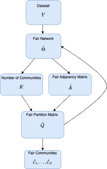
In this section, we consider a variant of (12) and provide a semidefinite programming approach for fair community detection. From (12), there is a feedback loop between $\Theta$ and the community structure ${\bf{Q}}$. The main justification for this is that it is important to know the communities of similar nodes, and this information should be taken into account in a direct way when estimating the graph matrix $\Theta$; see Figure  2(a).

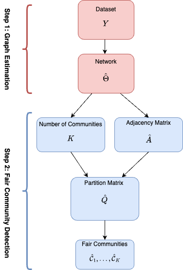
On the other hand, one might envision a simpler two-step sequential strategy where the communities are not taken into account when estimating the graph $\Theta$; see Figure 2(b). In this approach, in the first step, we estimate $\Theta$, and in the second step, we obtain the community partition matrix ${\bf{Q}}$. However, this approach has several limitations: First, it directly uses the empirical covariance, which is not consistent when the number of samples is smaller than the dimension. Secondly, there is no feedback from the communities to influence how the graph is estimated. Finally, $\hat{{\bf{A}}}$ is used as an observed adjacency matrix, and no variability in estimating $\hat{{\bf{A}}}$ is taken into account. Hence, in this sense, the communities, as well as the labeling of nodes, are not part of the model, and the estimation of graph similarity is not accounted for. The following two-step procedure provides the sequential estimation:

1. Iterate to obtain:

   $$~{}\hat{\mbox{\boldmath$\Theta$}}\leftarrow\underset{}{\text{argmin }}\hskip 5.69046ptL(\mbox{\boldmath$\Theta$};{\bf{Y}})+\rho_{1}\|\mbox{\boldmath$\Theta$}\|_{1,\textnormal{off}},~{}\text{ subj. to }~{}\mbox{\boldmath$\Theta$}\in\mathcal{M}.$$ (16)

2. Iterate to find:

   $$\min_{{\bf{Q}}}~{}\text{trace}(\hat{{\bf{E}}}{\bf{Q}})~{}\text{ subj. to }~{}{\bf{Q}}\in\mathcal{N},$$ (17)

   where

   $$\hat{{\bf{E}}} =-({\bf{I}}-\hat{{\bf{D}}})^{\frac{1}{2}}\hat{{\bf{A}}}({\bf{I}}-\hat{{\bf{D}}})^{\frac{1}{2}}+{\hat{{\bf{D}}}}^{\frac{1}{2}}({\bf{I}}-\hat{{\bf{A}}}){\hat{{\bf{D}}}}^{\frac{1}{2}}.$$

   Here, $\hat{{\bf{A}}}$ is an adjacency matrix with $\hat{a}_{ij}=1$ if $\hat{\theta}_{ij}\neq 0$ and $0$ otherwise; and ${\hat{{\bf{D}}}}$ is a diagonal matrix containing at its diagonal the degrees of the nodes in $\hat{{\bf{A}}}$.

In comparison with the optimization problem proposed in Section 2.2, we observe that the estimation in (16) can be performed using standard algorithms. Specifically, we can utilize a sparse graphical model to optimize (16) in Step T1.. Furthermore, our formulation in (17) provides a fair semidefinite programming variant of the procedure proposed in [17] for learning ${\bf{Q}}$ as stated in (17) in Step T2..

(a) Joint procedure

(b) Two-step procedure

Figure 2: Graphical models estimation and fair community detection.

The novelty of the approach in (12) comes from incorporating how the underlying community structure influences the estimation of the inverse covariance matrix. If one has knowledge that there are communities of nodes that group together due to functional resemblance, and thus tend to be more homogenous and ‘communicate’ more intensely with the members of their group, the proposed method incorporates this into the modeling step, and this is reflected in the estimation of $\boldsymbol{\Theta}$. In the two-step approach, this information is ignored.

2.4 Related Work

To the best of our knowledge, the fair graphical model proposed here is the first model that can jointly learn fair communities simultaneously with the structure of a conditional dependence network. Related work falls into two categories: graphical model estimation and fairness.

Estimation of graphical models.

There is a substantial body of literature on methods for estimating network structures from high-dimensional data, motivated by important biomedical and social science applications [71, 90, 49, 31, 38, 98, 45, 101]. Since in most applications the number of model parameters to be estimated far exceeds the available sample size, the assumption of sparsity is made and imposed through regularization of the learned graph. An $\ell_{1}$ penalty on the parameters encoding the network edges is the most common choice [38, 79, 57, 19, 108, 58, 85]. This approach encourages sparse uniform network structures that may not be the most suitable choice for real world applications, that may not be uniformly sparse. As argued in [31, 48, 101] many networks exhibit different structures at different scales. An example includes a densely connected subgraph or community in the social networks literature. Such structures in social interaction networks may correspond to groups of people sharing common interests or being co-located [101], while in biological systems to groups of proteins responsible for regulating or synthesizing chemical products and in precision medicine the communities may be patients with common disease suceptibilities. An important part of the literature therefore deals with the estimation of hidden communities of nodes, by which it is meant that certain nodes are linked more often to other nodes which are similar, rather than to dissimilar nodes. This way the nodes from communities that are more homogeneous within the community than between communities where there is a larger degree of heterogeneity. Some of the initial work focused on either inferring connectivity information [74] or performing graph estimation in case the connectivity or community information is known a priori [31, 48, 40, 72, 68], but not both tasks simultaneously. Recent developments consider the two tasks jointly and estimate the structured graphical models arising from heterogeneous observations [64, 54, 50, 101, 63, 41, 88, 21, 35].

Fairness.

There is a growing body of work on fairness in ML. Much of the research is on fair supervised methods; see, [30, 11, 34] and references therein. Our paper adds to the literature on fair methods for unsupervised learning tasks [29, 23, 92, 100, 82, 22, 59, 105]. We discuss the work on fairness most closely related to our paper. [29] provides approximation algorithms that incorporate this fairness notion into $K$-center as well as $K$-median clustering. [59] extend this to K-means and provide a provable fair spectral clustering method; they implement $K$-means on the subspace spanned by the smallest fair eigenvectors of Laplacian matrix. Unlike these works, which assume that the graph structure and/or the number of communities is given in advance, an appealing feature of our method is to learn fair community structure while estimating heterogeneous graphical models.

Convex Community Detection.

Convex optimization approaches for community detection can be traced back to the computer science and mathematical programming literature in the study of the planted partition problem; see, e.g., [76, 27, 6]. For community detection under statistical models, various theoretical properties of convex optimization methods have been studied in depth recently; a partial list includes strong consistency with a growing number of communities [25, 26, 18], sharp threshold under sparse networks for strong consistency [1, 9, 3], weak consistency [44, 37], non-trivial recovery [81, 78], robustness against outlier nodes [18], consistency under degree-corrected models [28], and consistency under weak associativity [7]. Motivated by this line of work, our work provides the first convex programming approach for detecting fair communities within a known graph. This approach retains the computational complexity of convex community detection methods [8, 17, 70] while enhancing fairness in community structure.

3 The Fair Community Detection and Graphical Models

In the following subsections, we consider two special cases of (12) that lead to estimation of graphical models for continuous and binary data.

3.1 Fair Pseudo-Likelihood Graphical Model

Suppose ${\bf{y}}_{i}=(y^{1}_{i},\ldots,y^{p}_{i})$ are i.i.d. observations from $N(\mbox{\boldmath$0$},\mbox{\boldmath$\Sigma$})$, for $i=1,\ldots,n$. Denote the sample of the $i$th variable as ${\bf{y}}^{i}=(y^{i}_{1},\ldots,y^{i}_{n})$. Let $\omega_{ij}:=-\theta_{ij}/\theta_{ii}$, for all $j\neq i$. We note that the set of nonzero coefficients of $\omega_{ij}$ is the same as the set of nonzero entries in the row vector of $\theta_{ij}~{}(i\neq j)$, which defines the set of neighbors of node $\theta_{ij}$. Using an $\ell_{1}$-penalized regression, [79] estimates the zeros in $\Theta$ by fitting separate Lasso regressions for each variable ${\bf{y}}^{i}$ given the other variables as follows

$$F_{i}(\mbox{\boldmath$\Theta$};{\bf{Y}})=\|{\bf y}^{i}-\sum_{j\neq i}\omega_{ij}{\bf y}^{j}\|^{2}+\rho_{1}\sum_{1\leq i<j\leq p}\left|\omega_{ij}\right|,~{}~{}\textnormal{where}~{}~{}\omega_{ij}=-\theta_{ij}/\theta_{ii}.$$ (18)

These individual Lasso fits give neighborhoods that link each variable to others. [85] improve this neighborhood selection method by taking the natural symmetry in the problem into account (i.e., $\theta_{ij}=\theta_{ij}$ ), and propose the following joint objective function (called SPACE):

$$F(\mbox{\boldmath$\Theta$};{\bf{Y}}) =\frac{1}{2}\sum_{i=1}^{p}\big{(}-n\log\theta_{ii}+w_{i}\|{\bf y}^{i}-\sum_{j\neq i}\dot{\omega}_{ij}\sqrt{\frac{\theta_{jj}}{\theta_{ii}}}{\bf y}^{j}\|^{2}\big{)}+\rho\sum_{1\leq i<j\leq p}\left|\dot{\omega}_{ij}\right|$$

$$=\frac{1}{2}\sum_{i=1}^{p}\big{(}-n\log\theta_{ii}+w_{i}\|{\bf y}^{i}+\sum_{j\neq i}\frac{\theta_{ij}}{\theta_{ii}}{\bf y}^{j}\|^{2}\big{)}+\rho_{1}\sum_{1\leq i<j\leq p}\left|\dot{\omega}_{ij}\right|,$$ (19)

where $\{w_{i}\}_{i=1}^{p}$ are nonnegative weights and $\dot{\omega}_{ij}=-\frac{\theta_{ij}}{\sqrt{\theta_{ii}\theta_{jj}}}$ denotes the partial correlation between the $i$th and $j$th variables for $1\leq i\neq j\leq p$. Note that $\dot{\omega}_{ij}=\dot{\omega}_{ji}$ for $i\neq j$.

It is shown in [58] that the above expression is not convex. Setting $w_{i}=\theta_{ii}^{2}$ and putting the $\ell_{1}$-penalty term on the partial covariances $\theta_{ij}$ instead of on the partial correlations $\dot{\omega}_{ij}$, they obtain a convex pseudo-likelihood approach with good model selection properties called CONCORD. Their objective takes the form

$$F(\mbox{\boldmath$\Theta$};{\bf{Y}}) =\sum_{i=1}^{p}\big{(}-n\log\theta_{ii}+\frac{1}{2}\|\theta_{ii}{\bf y}^{i}+\sum_{j\neq i}\theta_{ij}{\bf y}^{j}\|_{2}^{2}\big{)}+\rho_{1}\sum_{1\leq i<j\leq p}|\theta_{ij}|.$$ (20)

Note that the matrix version of the CONCORD objective can be obtained by setting $L(\mbox{\boldmath$\Theta$};{\bf{Y}})=n/2[-\log|\text{diag}(\mbox{\boldmath$\Theta$})^{2}|+\text{trace}({\bf{S}}\mbox{\boldmath$\Theta$}^{2})]$ in (5).

Our proposed fair graphical model formulation, called FCONCORD, is a fair version of CONCORD from (20). In particular, letting $G(\mbox{\boldmath$\Theta$})=\frac{n}{2}\mbox{\boldmath$\Theta$}^{2}$ and

$$\mathcal{M}=\left\{\mbox{\boldmath$\Theta$}\in{\mathbb{R}}^{p\times p}:~{}\theta_{ij}=\theta_{ji},\text{ and }\theta_{ii}>0,\mbox{ for every }1\leq i,j\leq p\right\},$$

in (12), our problem takes the form

$$\operatorname*{minimize}_{\mbox{\boldmath$\Theta$},~{}\mbox{\boldmath$Q$}}~{}~{} \frac{n}{2}\big{[}-\log|\text{diag}(\mbox{\boldmath$\Theta$})^{2}|+\operatorname{trace}\big{(}({\bf{S}}+\rho_{2}{\bf{Q}})\mbox{\boldmath$\Theta$}^{2}\big{)}\big{]}+\rho_{1}\|\mbox{\boldmath$\Theta$}\|_{1,\textnormal{off}}$$

subj. to $$\mbox{\boldmath$\Theta$}\in\mathcal{M}~{}~{}\text{and}~{}~{}{\bf{Q}}\in\mathcal{N}.$$ (21)

Here, $\mathcal{M}$ and $\mathcal{N}$ are the graph adjacency and fairness constraints, respectively.

Remark 2.

When $\rho_{2}=0$, i.e., without a fairness constant and the second trace term, the objective in (3.1) reduces to the objective of the CONCORD estimator, and is similar to those of SPACE [85], SPLICE [91], and SYMLASSO [39]. Our framework is a generalization of these methods to fair graph learning and community detection, when the demographic group representation holds.

Problem (3.1) can be solved using Algorithm 1. The update for $\Omega$ and $\Theta$ in S2. and S3. can be derived by minimizing

$$\Upsilon_{1,\gamma}(\mbox{\boldmath$\Omega$}) :=\frac{n\rho_{2}}{2}\operatorname{trace}\big{(}{\bf{Q}}\mbox{\boldmath$\Omega$}^{2}\big{)}+\rho_{1}\|\mbox{\boldmath$\Omega$}\|_{1,\textnormal{off}}+\frac{\gamma}{2}\left\|\mbox{\boldmath$\Theta$}-\mbox{\boldmath$\Omega$}+{\bf{W}}\right\|_{F}^{2},$$ (22a)

$$\Upsilon_{2,\gamma}(\mbox{\boldmath$\Theta$}) :=\frac{n}{2}\big{[}-\log|\text{diag}(\mbox{\boldmath$\Theta$})^{2}|+\operatorname{trace}\big{(}{\bf{S}}\mbox{\boldmath$\Theta$}^{2}\big{)}\big{]}+\frac{\gamma}{2}\left\|\mbox{\boldmath$\Theta$}-\mbox{\boldmath$\Omega$}+{\bf{W}}\right\|_{F}^{2},$$ (22b)

with respect to $\Omega$ and $\Theta$, respectively.

For $1\leq i\leq j\leq p$, define the matrix function ${\bf{T}}_{ij}:\mathcal{M}\rightarrow\mathcal{M}$ by

$${\bf{T}}_{ij}(\mbox{\boldmath$\Omega$}) \leftarrow\operatorname*{argmin}_{{\tilde{\mbox{\boldmath$\Omega$}}}}\big{\{}\Upsilon_{1,\gamma}({\tilde{\mbox{\boldmath$\Omega$}}}):~{}{\tilde{\omega}}_{kl}=\omega_{kl}\;\forall(k,l)\neq(i,j)\big{\}},$$ (23a)

$${\bf{T}}_{ij}(\mbox{\boldmath$\Theta$}) \leftarrow\operatorname*{argmin}_{{\tilde{\mbox{\boldmath$\Theta$}}}}\big{\{}\Upsilon_{2,\gamma}({\tilde{\mbox{\boldmath$\Theta$}}}):~{}{\tilde{\theta}}_{kl}=\theta_{kl}\;\forall(k,l)\neq(i,j)\big{\}}.$$ (23b)

For each $(i,j)$, ${\bf{T}}_{ij}(\mbox{\boldmath$\Omega$})$ and ${\bf{T}}_{ij}(\mbox{\boldmath$\Theta$})$ updates the $(i,j)$-th entry with the minimizer of (22a) and (22b) with respect to $\omega_{ij}$ and $\theta_{ij}$, respectively, holding all other variables constant. Given ${\bf{T}}_{ij}(\mbox{\boldmath$\Omega$})$ and ${\bf{T}}_{ij}(\mbox{\boldmath$\Theta$})$, the update for $\Omega$ and $\Theta$ in S2. and S3. can be obtained by a similar coordinate-wise descent algorithm proposed in [85, 58]. Closed form updates for ${\bf{T}}_{ij}(\mbox{\boldmath$\Omega$})$ and ${\bf{T}}_{ij}(\mbox{\boldmath$\Theta$})$ are provided in Lemma 3.

Lemma 3.

Set $\gamma_{n}:=\gamma n$. For all $1\leq i\leq p$, let

$$a_{i}:=s_{ii}+\gamma_{n},\qquad\qquad\quad b_{i}:=\sum_{j\neq i}\theta_{ij}s_{ij}+\gamma_{n}(w_{ii}-\omega_{ii}),$$

$$c_{i}:=\rho_{2}q_{ii}+\gamma_{n},\qquad\qquad d_{i}:=\rho_{2}\sum_{j\neq i}q_{ij}\omega_{ij}+\gamma_{n}(w_{ii}+\theta_{ii}).$$

Further, for $1\leq i<j\leq p$, let

$$a_{ij}:=(s_{ii}+s_{jj})+\gamma_{n},\quad\quad\quad b_{ij}:=\big{(}\sum_{j^{\prime}\neq j}\theta_{ij^{\prime}}s_{jj^{\prime}}+\sum_{i^{\prime}\neq i}\theta_{i^{\prime}j}s_{ii^{\prime}}\big{)}+\gamma_{n}(w_{ij}-\omega_{ij}),$$

$$c_{ij}:=\rho_{2}(q_{ii}+q_{jj})+\gamma_{n},\qquad d_{ij}:=\rho_{2}\big{(}\sum_{j^{\prime}\neq j}\omega_{ij^{\prime}}q_{jj^{\prime}}+\sum_{i^{\prime}\neq i}\omega_{i^{\prime}j}q_{ii^{\prime}}\big{)}+\gamma_{n}(w_{ij}+\theta_{ij}).$$

Then, for all $1\leq i\leq p$:

$$~{}~{}~{}~{}~{}~{}\big{(}{\bf{T}}_{ii}(\mbox{\boldmath$\Omega$})\big{)}_{ii} =\frac{-d_{i}}{c_{i}},\qquad\qquad\qquad\big{(}{\bf{T}}_{ii}(\mbox{\boldmath$\Theta$})\big{)}_{ii}=\frac{1}{2a_{i}}(-b_{i}+\sqrt{b_{i}^{2}+4a_{i}}),$$ (24a)

and for all $$1\leq i<j\leq p$$:

$$\big{(}{\bf{T}}_{ij}(\mbox{\boldmath$\Omega$})\big{)}_{ij} =S\big{(}-\frac{d_{ij}}{c_{ij}},\frac{\rho_{1}}{\gamma_{n}}\big{)},\quad~{}~{}~{}~{}~{}\big{(}{\bf{T}}_{ij}(\mbox{\boldmath$\Theta$})\big{)}_{ij}=-\frac{b_{ij}}{a_{ij}},$$ (24b)

where $S(\alpha,\beta):=\textnormal{sign}(\alpha)\max(|\alpha|-\beta,0)$.

Note that alternatively, one can minimize the augmented Lagrangian function (14) and subproblem (22a) over $\Upsilon_{1,\gamma}(\mbox{\boldmath$\Omega$})-\log|\text{diag}(\mbox{\boldmath$\Omega$})^{2}|$. The additional term ensures that $\omega_{ii}>0$ at each iteration of the ADMM algorithm. In this case, the coordinate-descent update for $\big{(}{\bf{T}}_{ii}(\mbox{\boldmath$\Omega$})\big{)}_{ii}$ in (24a) becomes

$$\left({\bf{T}}_{ii}(\mbox{\boldmath$\Omega$})\right)_{ii}=\frac{1}{2c_{i}}\left(-d_{i}+\sqrt{d_{i}^{2}+4c_{i}}\right).$$

Remark 4.

In the case when $K$ and $H$ are known, the complexity of Step S1. in Algorithm 1 is of the same order as the CONCORD estimator, SPACE and SYMLASSO. In fact, computing the fair clustering matrix ${\bf{Q}}$ requires $O((p-H+1)^{2}K)$ operations. On the other hand, it follows from [58, Lemma 5] that the $\Theta$ updates can be performed with complexity $\min\left(O(np^{2}),O(p^{3})\right)$. This shows that when the number of communities is known, the computational cost of each iteration of FCONCORD is $\max\left(\min\left(O(np^{2}),O(p^{3})\right),(p-H+1)^{2}K\right)$.

Note that Eq (11) provides a unifying framework which includes a fair variant of the graphical Lasso, SPACE, SPLICE, and SYMLASSO. In particular, letting $L(\mbox{\boldmath$\Theta$};{\bf{Y}})=n/2[-\log\det(\mbox{\boldmath$\Theta$})+\operatorname{trace}({\bf{S}}\mbox{\boldmath$\Theta$})]$, $G(\mbox{\boldmath$\Theta$})=n/2\mbox{\boldmath$\Theta$}$, and $\mathcal{M}=\{\mbox{\boldmath$\Theta$}:\mbox{\boldmath$\Theta$}\succ 0~{}\text{ and}~{}\mbox{\boldmath$\Theta$}=\mbox{\boldmath$\Theta$}^{\top}\}$, we obtain

$$\operatorname*{minimize}_{\mbox{\boldmath$\Theta$},~{}\mbox{\boldmath$Q$}}~{}~{} \frac{n}{2}\big{[}-\log\det\mbox{\boldmath$\Theta$}+\operatorname{trace}\big{(}({\bf{S}}+\rho_{2}{\bf{Q}})\mbox{\boldmath$\Theta$}\big{)}\big{]}+\rho_{1}\|\mbox{\boldmath$\Theta$}\|_{1,\textnormal{off}}$$

subj. to $$\mbox{\boldmath$\Theta$}\in\mathcal{M}~{}~{}\text{and}~{}~{}{\bf{Q}}\in\mathcal{N},$$ (25)

which can be considered as a fair variant of cluster-based graphical Lasso [64, 54, 50, 41, 88, 21, 35].

3.1.1 Large Sample Properties of FCONCORD

We show that under suitable conditions, the FCONCORD estimator achieves both model selection consistency and estimation consistency.

As in other studies [58, 85], for the convergence analysis we assume that the diagonal of the graph matrix $\Theta$ and partition matrix ${\bf{Q}}$ are known. Let $\mbox{\boldmath$\theta$}^{o}=(\theta_{ij})_{1\leq i<j\leq p}$ and ${\bf{q}}^{o}=(q_{ij})_{1\leq i<j\leq p}$ denote the vector of off-diagonal entries of $\Theta$ and ${\bf{Q}}$, respectively. Let $\mbox{\boldmath$\theta$}^{d}$ and ${\bf{q}}^{d}$ denote the vector of diagonal entries of $\Theta$ and ${\bf{Q}}$, respectively. Let $\bar{\mbox{\boldmath$\theta$}}^{o},\bar{\mbox{\boldmath$\theta$}}^{d},\bar{{\bf{q}}}^{o}$, and $\bar{{\bf{q}}}^{d}$ denote the true value of ${\mbox{\boldmath$\theta$}}^{o},{\mbox{\boldmath$\theta$}}^{d},{\bf{q}}^{o}$, and ${\bf{q}}^{d}$, respectively. Let $\mathcal{B}$ denote the set of non-zero entries in the vector $\bar{\mbox{\boldmath$\theta$}}^{o}$ and define

$$q :=|\mathcal{B}|,~{}~{}~{}~{}\Psi(p,H,K):=(p-H+1)((p-H+1)/K-1).$$ (26)

In our consistency analysis, we let the regularization parameters $\rho_{1}=\rho_{1n}$ and $\rho_{2}=\rho_{2n}$ vary with $n$.

The following standard assumptions are required:
Assumption A

1. The random vectors ${\bf{y}}_{1},\dots,{\bf{y}}_{n}$ are i.i.d. sub-Gaussian for every $n\geq 1$, i.e., there exists $\tau>0$ such that $\|{\bf{u}}^{\top}{\bf{y}}_{i}\|_{\psi_{2}}\leq\tau\sqrt{{\mathbb{E}}({\bf{u}}^{\top}{\bf{y}}_{i})^{2}}$, $\forall{\bf{u}}\in{\mathbb{R}}^{p}$. Here, $\|{\bf{y}}\|_{\psi_{2}}=\sup_{t\geq 1}({\mathbb{E}}|{\bf{y}}|^{t})^{\frac{1}{t}}/\sqrt{t}$.

2. There exist constants $\tau_{1},\tau_{2}\in(0,\infty)$ such that

   $$\tau_{1}<\Lambda_{\min}(\bar{\mbox{\boldmath$\Theta$}})\leq\Lambda_{\max}(\bar{\mbox{\boldmath$\Theta$}})<\tau_{2}.$$

3. There exists a constant $\tau_{3}\in(0,\infty)$ such that

   $$0\leq\Lambda_{\min}(\bar{{\bf{Q}}})\leq\Lambda_{\max}(\bar{{\bf{Q}}})<\tau_{3}.$$

4. For any $K,H\in[p]$, we have $K\leq p-H+1$.

5. There exists a constant $\delta\in(0,1]$ such that, for any $(i,j)\in\mathcal{B}^{c}$

   $$\left|\bar{{\bf{H}}}_{ij,\mathcal{B}}\bar{{\bf{H}}}_{\mathcal{B},\mathcal{B}}^{-1}\operatorname{sign}(\bar{\mbox{\boldmath$\theta$}}^{o}_{\mathcal{B}})\right|\leq(1-\delta),$$

   where for $1\leq i,j,t,s\leq p$ satisfying $i<j$ and $t<s$,

   $$\bar{{\bf{H}}}_{ij,ts}:={\mathbb{E}}_{\bar{\mbox{\boldmath$\theta$}}^{o}}\Big{(}\frac{\partial^{2}L(\bar{\mbox{\boldmath$\theta$}}^{d},{\mbox{\boldmath$\theta$}}^{o};{\bf{Y}})}{\partial\theta_{ij}\partial\theta_{ts}}\Big{|}_{\mbox{\boldmath$\theta$}^{o}=\bar{\mbox{\boldmath$\theta$}}^{o}}\Big{)}.$$ (27)

Assumptions (A2)–(A3) guarantee that the eigenvalues of the true graph matrix $\bar{\mbox{\boldmath$\Theta$}}$ and those of the true membership matrix $\bar{{\bf{Q}}}$ are well-behaving. Assumption (A4) links how $H,K$ and $p$ can grow with $n$. Note that $K$ is limited in order for fairness constraints to be meaningful; if $K>p-H+1$ then there can be no community with $H$ nodes among which we enforce fairness. Assumption (A5) corresponds to the incoherence condition in [79], which plays an important role in proving model selection consistency of $\ell_{1}$ penalization problems. [113] show that such a condition is almost necessary and sufficient for model selection consistency in Lasso regression, and they provide some examples when this condition is satisfied. Note that Assumptions (A1), (A2), and (A5) are identical to Assumptions (C0)–(C2) in [85]. Further, it follows from [85] that under Assumption (A5) for any $(i,j)\in\mathcal{B}^{c}$,

$$\|\bar{{\bf{H}}}_{ij,\mathcal{B}}\bar{{\bf{H}}}_{\mathcal{B},\mathcal{B}}^{-1}\|\leq M(\bar{\mbox{\boldmath$\theta$}}^{o})$$ (28)

for some finite constant $M(\bar{\mbox{\boldmath$\theta$}}^{o})$.

Next, inspired by [85, 58], we prove estimation consistency for the nodewise FCONCORD.

Theorem 5.

Suppose Assumptions (A1)–(A5) are satisfied. Assume further that $p=O(n^{\kappa})$ for some $\kappa>0$, $\rho_{1n}=O(\sqrt{\log p/n})$, $n>O(q\log(p))$ as $n\rightarrow\infty$, $\rho_{2n}=O(\sqrt{\log(p-H+1)/n})$, $\rho_{2n}\leq\delta\rho_{1n}/((1+M(\bar{\mbox{\boldmath$\theta$}}^{o}))\tau_{2}\tau_{3})$, and $\mbox{\boldmath$\epsilon$}=\mbox{\boldmath$0$}$. Then, there exist finite constants $C(\bar{\mbox{\boldmath$\theta$}}^{o})$ and $D(\bar{{\bf{q}}}^{o})$, such that for any $\eta>0$, the following events hold with probability at least $1-O(\exp(-\eta\log p))$:

• There exists a minimizer $({\widehat{\mbox{\boldmath$\theta$}}}^{o},{\widehat{{\bf{q}}}}^{o})$ of (3.1) such that

  $$\max\big{(}\|\widehat{\mbox{\boldmath$\theta$}}^{o}-\bar{\mbox{\boldmath$\theta$}}^{o}\|,\|{\widehat{{\bf{q}}}}^{o}-\bar{{\bf{q}}}^{0}\|\big{)}\\ \leq\max\big{(}C(\bar{\mbox{\boldmath$\theta$}}^{o})\rho_{1n}\sqrt{q},D(\bar{{\bf{q}}}^{o})\rho_{2n}\sqrt{\Psi(p,H,K)}\big{)},$$

  where $q$ and $\Psi(p,H,K)$ are defined in (26).

• If $\min_{(i,j)\in\mathcal{B}}\bar{\theta}_{ij}\geq 2C(\bar{\mbox{\boldmath$\theta$}}^{o})\rho_{1n}\sqrt{q}$, then ${\widehat{\mbox{\boldmath$\theta$}}}^{o}_{\mathcal{B}^{c}}=0$.

Theorem 5 provides sufficient conditions on the quadruple $(n,p,H,K)$ and the model parameters for the FCONCORD to succeed in consistently estimating the neighborhood of every node in the graph and communities simultaneously. Notice that if $H=1$ (no fairness) and $K=p$ (no clustering) we recover the results of [58, 85].

3.2 Fair Ising Graphical Model

In the previous section, we studied the fair estimation of graphical models for continuous data. Next, we focus on estimating an Ising Markov random field [55], suitable for binary or categorical data. Let ${\bf{y}}=(y_{1},\ldots,y_{p})\in\{0,1\}^{p}$ denote a binary random vector. The Ising model specifies the probability mass function

$$p({\bf{y}})=\frac{1}{\mathcal{W}(\mbox{\boldmath$\Theta$})}\exp\Big{(}\sum_{j=1}^{p}\theta_{jj}y_{j}+\sum_{1\leq j<j^{\prime}\leq p}\theta_{jj^{\prime}}y_{j}y_{j^{\prime}}\Big{)}.$$ (29)

Here, $\mathcal{W}(\mbox{\boldmath$\Theta$})$ is the partition function, which ensures that ensures that the density function in (29) integrates to one; $\Theta$ is a $p\times p$ symmetric matrix that specifies the graph structure: $\theta_{jj^{\prime}}=0$ implies that the $j$th and $j^{\prime}$th variables are conditionally independent given the remaining ones.

Several sparse estimation procedures for this model have been proposed. [67] considered maximizing an $\ell_{1}$-penalized log-likelihood for this model. Due to the difficulty in computing the log-likelihood with the expensive partition function, alternative approaches have been considered. For instance, [89] proposed a neighborhood selection approach which involves solving $p$ logistic regressions separately (one for each node in the network), which leads to an estimated parameter matrix that is in general not symmetric. In contrast, others have considered maximizing an $\ell_{1}$-penalized pseudo-likelihood with a symmetric constraint on $\Theta$ [49, 47, 98, 101]. Under the probability model above, the negative $\log$-pseudo-likelihood for $n$ observations takes the form

$$L(\mbox{\boldmath$\Theta$};{\bf{Y}})=-\sum_{j=1}^{p}\sum_{j^{\prime}=1}^{p}\theta_{jj^{\prime}}s_{jj^{\prime}}+\frac{1}{n}\sum_{i=1}^{n}\sum_{j=1}^{p}\log\big{(}1+\exp(\theta_{jj}+\sum_{j^{\prime}\neq j}\theta_{jj^{\prime}}y_{ij^{\prime}})\big{)}.$$ (30)

We propose to additionally impose the fairness constraints on $\Theta$ in (30) in order to obtain a sparse binary network with fair clustering. Let $\mathcal{M}=\{\mbox{\boldmath$\Theta$}\in{\mathbb{R}}^{p\times p}:~{}\mbox{\boldmath$\Theta$}=\mbox{\boldmath$\Theta$}^{\top}\}$, $G(\mbox{\boldmath$\Theta$})=n/2\mbox{\boldmath$\Theta$}^{2}$ and choose $\iota_{n}\in(0,1)$ such that $n\iota_{n}\rightarrow 0$ as $n\rightarrow\infty$. Under this setting, we consider the following criterion

$$\operatorname*{minimize}_{\mbox{\boldmath$\Theta$},\mbox{\boldmath$Q$}}~{}~{}~{}~{}~{}~{} \sum_{j=1}^{p}\sum_{j^{\prime}=1}^{p}-n\theta_{jj^{\prime}}s_{jj^{\prime}}+\frac{\rho_{2}n}{2}\operatorname{trace}\big{(}({\bf{Q}}+\iota_{n}{\bf{I}})\mbox{\boldmath$\Theta$}^{2}\big{)}$$

$$+\sum_{i=1}^{n}\sum_{j=1}^{p}\log\big{(}1+\exp(\theta_{jj}+\sum_{j^{\prime}\neq j}\theta_{jj^{\prime}}y_{ij^{\prime}})\big{)}+\rho_{1}\sum_{1\leq i<j\leq p}|\theta_{ij}|,$$

subj. to $$\mbox{\boldmath$\Theta$}\in\mathcal{M}~{}~{}\text{and}~{}~{}{\bf{Q}}\in\mathcal{N}.$$ (31)

Here, $\mathcal{M}$ and $\mathcal{N}$ are the graph and fairness constraints, respectively. Note that $\iota_{n}$ is used to provide a theoretical guarantee of convergence to a local minimum and throughout all numerical experiments is set to zero; see, Lemma 19 in Appendix for further details.

We refer to the solution to (3.2) as the Fair Binary Network (FBN). An interesting connection can be drawn between our technique and a fair variant of Ising block model discussed in [13], which is a perturbation of the mean field approximation of the Ising model known as the Curie-Weiss model: the sites are partitioned into two blocks of equal size and the interaction between those within the same block is stronger than across blocks, to account for more order within each block.

An ADMM algorithm for solving (3.2) is given in Algorithm 1. The update for $\Omega$ in S2. can be obtained from (22a) by replacing $\mbox{\boldmath$\Omega$}^{2}$ with $\Omega$. We solve the update for $\Theta$ in S3. using a relaxed variant of Barzilai-Borwein method [12]. The details are given in [101, Algorithm 2].

3.2.1 Large Sample Properties of FBN

In this section, we present the model selection consistency property for the Ising model. The spirit of the proof is similar to [89], but their model does not include membership matrix ${\bf{Q}}$ and fairness constraints.

Similar to Section 3.1.1, let $\mbox{\boldmath$\theta$}^{o}=(\theta_{ij})_{1\leq i<j\leq p}$ and ${\bf{q}}^{o}=(q_{ij})_{1\leq i<j\leq p}$ denote the vector of off-diagonal entries of $\Theta$ and ${\bf{Q}}$, respectively. Let $\mbox{\boldmath$\theta$}^{d}$ and ${\bf{q}}^{d}$ denote the vector of diagonal entries of $\Theta$ and ${\bf{Q}}$, respectively. Let $\bar{\mbox{\boldmath$\theta$}}^{o},\bar{\mbox{\boldmath$\theta$}}^{d},\bar{{\bf{q}}}^{o},\bar{{\bf{q}}}^{d}$, $\bar{\mbox{\boldmath$\Theta$}}$ and $\bar{{\bf{Q}}}$ denote the true value of ${\mbox{\boldmath$\theta$}}^{o},{\mbox{\boldmath$\theta$}}^{d},{\bf{q}}^{o},{\bf{q}}^{d}$, $\Theta$ and ${\bf{Q}}$, respectively. Let $\mathcal{B}$ denote the set of non-zero entries in the vector $\bar{\theta}^{o}$, and let $q=|\mathcal{B}|$. Denote the log-likelihood for the $i$-th observation by

$$L_{i}(\mbox{\boldmath$\theta$}^{d},{\mbox{\boldmath$\theta$}}^{o};{\bf{Y}})=-\sum_{j=1}^{p}y_{ij}\big{(}\theta_{jj}+\sum_{j\neq j^{\prime}}\theta_{jj^{\prime}}y_{ij^{\prime}}\big{)}+\log\big{(}1+\exp(\mbox{\boldmath$\theta$}_{jj}\sum_{j\neq j^{\prime}}\theta_{jj^{\prime}}y_{ij^{\prime}})\big{)}.$$ (32)

The population Fisher information matrix of $L$ at $(\bar{\mbox{\boldmath$\theta$}}^{d},\bar{\mbox{\boldmath$\theta$}}^{o})$ can be expressed as $\bar{{\bf{H}}}={\mathbb{E}}(\nabla^{2}L_{i}(\bar{\mbox{\boldmath$\theta$}}^{d},\bar{\mbox{\boldmath$\theta$}}^{o};{\bf{Y}}))$. Further, its sample counterpart is defined as $\bar{{\bf{H}}}^{n}=1/n\sum_{i=1}^{n}\nabla^{2}L_{i}(\bar{\mbox{\boldmath$\theta$}}^{d},\bar{\mbox{\boldmath$\theta$}}^{o};{\bf{Y}})$. Let

$$v_{ij} =\dot{v}_{ij}(1-\dot{v}_{ij}),~{}~{}\textnormal{where}~{}~{}\dot{v}_{ij}=\frac{\exp(\theta_{jj}+\sum_{j^{\prime}\neq j}\theta_{jj^{\prime}}y_{ij^{\prime}})}{1+\exp(\theta_{jj}+\sum_{j^{\prime}\neq j}\theta_{jj^{\prime}}y_{ij^{\prime}})},~{}~{}\textnormal{and}$$

$$\widetilde{{\bf{y}}}_{j} =\left(\sqrt{v_{1j}}y_{1j}-\dot{{\bf{y}}}_{j},\ldots,\sqrt{v_{nj}}y_{nj}-\dot{{\bf{y}}}_{j}\right)^{\top},~{}~{}\textnormal{where}~{}~{}\dot{{\bf{y}}}_{j}=1/n\sum_{i=1}^{n}\sqrt{v_{ij}}y_{ij}.$$

We use $\tilde{{\bf{X}}}=(\tilde{{\bf{X}}}_{(1,2)},\cdots,\tilde{{\bf{X}}}_{(p-1,p)})$ to denote an $np$ by $p(p-1)/2$ matrix, with

$$\tilde{{\bf{X}}}_{(j,j^{{}^{\prime}})}=\Big{(}{\bf{0}}_{n},...,{\bf{0}}_{n},\underbrace{\widetilde{{\bf{y}}}_{j}}_{j-\textnormal{th block}},{\bf{0}}_{n},...,{\bf{0}}_{n},\underbrace{\widetilde{{\bf{y}}}_{j^{{}^{\prime}}}}_{j^{{}^{\prime}}-\textnormal{th block}},{\bf{0}}_{n},\ldots,{\bf{0}}_{n}\Big{)}^{\top},$$

where ${\bf{0}}_{n}$ is an $n$-dimensional column vector of zeros. Let $\tilde{{\bf{X}}}^{(i,j)}$ be the $[(j-1)n+i]$-th row of $\tilde{{\bf{X}}}$ and $\tilde{{\bf{X}}}^{(i)}=(\tilde{{\bf{X}}}^{(i,1)},\ldots,\tilde{{\bf{X}}}^{(i,p)})$. Let ${\bf{T}}={\mathbb{E}}(\tilde{{\bf{X}}}^{(i)}(\tilde{{\bf{X}}}^{(i)})^{\top})$ and ${\bf{T}}^{n}=1/n\sum_{i=1}^{n}\tilde{{\bf{X}}}^{(i)}(\tilde{{\bf{X}}}^{(i)})^{\top}$ as its sample counterpart.

Our results rely on Assumptions (A2)–(A4) and the following regularity conditions:
Assumption B

1. There exist constants $\tau_{2},\tau_{4},\tau_{5}\in(0,\infty)$ such that $\Lambda_{\max}(\bar{\mbox{\boldmath$\Theta$}})<\tau_{2}$, and

   $$\Lambda_{\min}(\bar{{\bf{H}}}_{\mathcal{B}\mathcal{B}})\geq\tau_{4}~{}~{}~{}\text{and}~{}~{}~{}\Lambda_{\max}({\bf{T}})\leq\tau_{5}.$$

2. There exists a constant $\delta\in(0,1]$, such that

   $$\|\bar{{\bf{H}}}_{\mathcal{B}^{c}\mathcal{B}}\left(\bar{{\bf{H}}}_{\mathcal{B}\mathcal{B}}\right)^{-1}\|_{\infty}\leq(1-\delta).$$ (33)

It should be mentioned that Assumptions (B1)-(B2) are similar to those listed in [89, 46]. Under these assumptions and (A2)–(A4), we have the following result:

Theorem 6.

Suppose Assumptions (A2)–(A4) and (B1)–(B2) are satisfied. Assume further that $\rho_{1n}=O(\sqrt{\log p/n})$, $n>O(q^{3}\log p)$ as $n\rightarrow\infty$, $\rho_{2n}=O(\sqrt{\log(p-H+1)/n})$, $\rho_{2n}\leq\delta\rho_{1n}/(4(2-\delta)\tau_{2}\tau_{3})$, and $\mbox{\boldmath$\epsilon$}=\mbox{\boldmath$0$}$. Then, there exist finite constants $\check{C}(\bar{\mbox{\boldmath$\theta$}}^{o})$, $\check{D}(\bar{{\bf{q}}}^{o})$, and $\eta$ such that the following events hold with probability at least $1-O(\exp(-\eta\rho_{1n}^{2}n))$:

• There exists a local minimizer $({\widehat{\mbox{\boldmath$\theta$}}}^{o},{\widehat{{\bf{q}}}}^{o})$ of (3.2) such that

  $$\max\left(\|\widehat{\mbox{\boldmath$\theta$}}^{o}-\bar{\mbox{\boldmath$\theta$}}^{o}\|,\|{\widehat{{\bf{q}}}}^{o}-\bar{{\bf{q}}}^{0}\|\right)$$

  $$\qquad\leq\max\left(\check{C}(\bar{\mbox{\boldmath$\theta$}}^{o})\rho_{1n}\sqrt{q},\check{D}(\bar{{\bf{q}}}^{o})\rho_{2n}\sqrt{\Psi(p,H,K)}\right),$$ (34)

  where $q$ and $\Psi(p,H,K)$ are defined in (26).

• If $\min_{(i,j)\in\mathcal{B}}\bar{\theta}_{ij}^{o}\geq 2\check{C}(\bar{\mbox{\boldmath$\theta$}}^{o})\sqrt{q}\rho_{1n}$, then ${\widehat{\mbox{\boldmath$\theta$}}}^{o}_{\mathcal{B}^{c}}=0$.

Theorem 6 gives sufficient conditions on the quadruple $(n,p,H,K)$ and the model parameters for the FBN to succeed in consistently estimating the neighborhood of every node in the graph and communities simultaneously. In the case when $H=1$ (no fairness) and $K=p$ (no clustering), we recover the results of [89].

3.3 Consistency of Fair Community Labeling in Graphical Models

In this section, we aim to show that our algorithms recover the fair ground-truth community structure in the graph. Let ${\widehat{{\bf{V}}}}$ and $\bar{{\bf{V}}}$ contain the orthonormal eigenvectors corresponding to the $K$ leading eigenvalues of ${\widehat{{\bf{Q}}}}$ and $\bar{{\bf{Q}}}$ as columns, respectively. It follows from [69, Lemma 2.1] that if any rows of the matrix $\bar{{\bf{V}}}$ are same, then the corresponding nodes belong to the same cluster. Consequently, we want to show that up to some orthogonal transformation, the rows of ${\widehat{{\bf{V}}}}$ are close to the rows of $\bar{{\bf{V}}}$ so that we can simply apply K-means clustering to the rows of the matrix ${\widehat{{\bf{V}}}}$. In particular, we consider the K-means approach [69] defined as

$$({\widehat{{\bf{U}}}},{\widehat{{\bf{O}}}})=\operatorname*{argmin}_{{\bf{U}},{\bf{O}}}\|{\bf{U}}{\bf{O}}-{\widehat{{\bf{V}}}}\|_{\textnormal{F}}^{2},~{}~{}\text{subject to}~{}~{}{\bf{U}}\in\mathbb{M}_{p,K},~{}~{}{\bf{O}}\in{\mathbb{R}}^{K\times K},$$ (35)

where $\mathbb{M}_{p,K}$ is the set of $p\times K$ matrices that have on each row a single $1$, indicating the fair community to which the node belongs, and all other values on the row set at $0$, since a node belongs to only one community.

Finding a global minimizer for the problem (35) is NP-hard [5]. However, there are polynomial time approaches [62] that find an approximate solution $({\widehat{{\bf{U}}}},{\widehat{{\bf{O}}}})\in\mathbb{M}_{p,K}\times{\mathbb{R}}^{K\times K}$ such that

$$\|{\widehat{{\bf{U}}}}{\widehat{{\bf{O}}}}-{\widehat{{\bf{V}}}}\|_{\textnormal{F}}^{2}\leq(1+\xi)\operatorname*{argmin}_{({\bf{U}},{\bf{O}})\in\mathbb{M}_{p,K}\times{\mathbb{R}}^{K\times K}}\|{\bf{U}}{\bf{O}}-{\widehat{{\bf{V}}}}\|_{\textnormal{F}}^{2}.$$ (36)

Next, similar to [69, Theorem 3.1], we quantify the errors when performing $(1+\xi)$-approximate K-means clustering on the rows of $\widehat{{\bf{V}}}$ to estimate the community membership matrix. To do so, let $\mathcal{E}_{k}$ denote the set of misclassified nodes from the $k$-th community. By $\bar{\mathcal{C}}=\cup_{k\in[K]}({\mathcal{C}_{k}}\backslash{\mathcal{E}_{k}})$ we denote the set of all nodes correctly classified across all communities and by $\bar{{\bf{V}}}_{\bar{\mathcal{C}}}$ we denote the submatrix of $\bar{{\bf{V}}}$ formed by retaining only the rows indexed by the set $\bar{\mathcal{C}}$ of correctly classified nodes and all columns. Theorem 7 relates the sizes of the sets of misclassified nodes for each fair community and specify conditions on the interplay between $n$, $p$, $H$, and $K$.

Theorem 7.

Let ${\widehat{{\bf{U}}}}$ be the output of $(1+\xi)$-approximate K-means given in (36). If

$$(2+\xi)\Psi(p,H,K)\sqrt{\frac{K}{n}}<\pi$$

for some constant $\pi>0$, then there exist subsets $\mathcal{E}_{k}\subset\mathcal{C}_{k}$ for $k=1,\ldots,K$, and a permutation matrix $\Phi$ such that ${\widehat{{\bf{V}}}}_{\bar{\mathcal{C}}}\mbox{\boldmath$\Phi$}=\bar{{\bf{V}}}_{\bar{\mathcal{C}}}$, and

$$\sum_{k=1}^{K}|\mathcal{E}_{k}|/|\mathcal{C}_{k}|\leq\pi^{-1}(2+\xi)\Psi(p,H,K)\sqrt{\frac{K}{n}}$$

with probability tending to 1.

4 Simulation Study

4.1 Tuning Parameter Selection

We consider a Bayesian information criterion (BIC)-type quantity for tuning parameter selection in (11). Recall from Section 2.1 that objective function (11) decomposes the parameter of interest into $(\mbox{\boldmath$\Theta$},{\bf{Q}})$ and places $\ell_{1}$ and trace penalties on $\Theta$ and ${\bf{Q}}$, respectively. Specifically, for the graphical Lasso, i.e., problem in (11) with $\rho_{2}=0$, [112] proposed to select the tuning parameter $\rho_{1}$ such that $\hat{\mbox{\boldmath$\Theta$}}$ minimizes the following quantity:

$$n\left(-\log\det(\hat{\mbox{\boldmath$\Theta$}})+\cdot\text{trace}(\mbox{\boldmath$S$}\hat{\mbox{\boldmath$\Theta$}})\right)+\log(n)\cdot|\hat{\mbox{\boldmath$\Theta$}}|.$$

Here, $|\hat{\mbox{\boldmath$\Theta$}}|$ is the cardinality of $\hat{\mbox{\boldmath$\Theta$}}$, i.e., the number of unique non-zeros in $\hat{\mbox{\boldmath$\Theta$}}$. Note that $\rho_{1}$ controls the sparsity of the inferred graph and that the dependency of the criterion comes through the estimator $\hat{\mbox{\boldmath$\Theta$}}$.

Using a similar idea, we consider minimizing the following BIC-type criteria for selecting the set of tuning parameters $(\rho_{1},\rho_{2})$ for (11):

$$\mathrm{BIC}(\hat{\mbox{\boldmath$\Theta$}},\hat{{\bf{Q}}}):=\sum_{k=1}^{K} n_{k}\left(-\log|\hat{\mbox{\boldmath$\Theta$}}_{k}^{2}|+\text{trace}\left(\left({\bf{S}}_{k}+c\hat{{\bf{Q}}}_{k}\right)\hat{\mbox{\boldmath$\Theta$}}_{k}^{2}\right)\right)$$

$$+\log(n_{k})\cdot|\hat{\mbox{\boldmath$\Theta$}}_{k}|,$$ (37)

where $\hat{\mbox{\boldmath$\Theta$}}_{k}$ is the $k$-th estimated inverse covariance matrix.

Note that when the constant $c$ is small, the $\mathrm{BIC}(\hat{\mbox{\boldmath$\Theta$}},\hat{{\bf{Q}}})$ will be more influenced by graph estimation than fair community detection. Throughout, we take $c=0.25$. Other parameters of the algorithm are set to $\gamma=1e-2$ and $\nu=1e-4$.

4.2 Notation and Measures of Performance

We define several measures of performance that will be used to numerically compare the various methods. To assess the clustering performance, we compute the clustering error (CE) and Ratio Cut (RCut) [103]. CE calculates the distance between an estimated community assignment $\hat{z}_{i}$ and the true assignment $z_{i}$ of the $i$th node:

$$\textnormal{CE}:=\frac{1}{p}\left|\left\{(i,j):{\bf{1}}(\hat{z}_{i}=\hat{z}_{j})\neq{\bf{1}}(z_{i}=z_{j}),i<j\right\}\right|.$$

For a clustering $\mathcal{V}=\mathcal{C}_{1}{\cup}\ldots{\cup}\mathcal{C}_{K}$, we have

$$\text{RCut}:=\sum_{k=1}^{K}\frac{\text{Cut}(\mathcal{C}_{k},\mathcal{V}\setminus\mathcal{C}_{k})}{|\mathcal{C}_{k}|},~{}~{}~{}\text{Cut}(\mathcal{C}_{k},\mathcal{V}\setminus\mathcal{C}_{k}):=\sum_{i\in\mathcal{C}_{k},j\in\mathcal{V}\setminus\mathcal{C}_{k}}\theta_{ij}.$$

To measure the estimation quality, we calculate the proportion of correctly estimated edges (PCEE) [101]:

$$\textnormal{PCEE}:=\frac{\sum_{j^{\prime}<j}\left(1_{\{|\hat{\theta}_{jj^{\prime}}|>10^{-5}\text{ and }|\theta_{jj^{\prime}}|\neq 0\}}\right)}{\sum_{j^{\prime}<j}\left(1_{\{|\theta_{jj^{\prime}}|\neq 0\}}\right)}.$$

Finally, we use balance as a fairness metric to reflect the distribution of the fair clustering [29]. Let $\mathcal{N}_{i}=\{j:r_{ij}=1\}$ be the set of neighbors of node $i$ in ${\bf{R}}$. For a set of communities $\{\mathcal{C}_{k}\}_{k=1}^{K}$, the balance coefficient is defined as

$$\textnormal{Balance}:=\frac{1}{p}\sum_{i=1}^{p}\tau_{i}~{}~{}~{}\textnormal{where}~{}~{}~{}\tau_{i}=\min_{k,\ell\in[K]}\frac{|\mathcal{C}_{k}\cap\mathcal{N}_{i}|}{|\mathcal{C}_{\ell}\cap\mathcal{N}_{i}|}.$$ (38)

Note that $0\leq\tau_{i}\leq 1$, and a large $\tau_{i}$ indicates that node $i$ has an adequate representation in all communities. In particular, the balance is used to quantify how well the selected edges can eliminate discrimination–the selected edges are considered fairer if they can lead to a balanced community structure that preserves proportions of protected attributes.

4.3 Data Generation

In order to demonstrate the performance of the proposed algorithms, we create several synthetic datasets based on a special random graph with community and group structures. Then the baseline and proposed algorithms are used to recover graphs (i.e., graph-based models) from the artificially generated data. To create a dataset, we first construct a graph, then its associated adjacency matrix, $\Theta$, is used to generate independent data samples from the distribution $N(0,\mbox{\boldmath$\Theta$}^{\dagger})$ where $\dagger$ denotes pseudoinverse. A graph (i.e., $\Theta$) is constructed in two steps.

In the first step, we determine the graph structure (i.e., connectivity) based on the random modular graph also known as stochastic block model (SBM) [53, 69]. The stochastic block model [53] is a generative model for random graphs with planted blocks (ground-truth clustering). It is widely used to generate synthetic networks containing communities, subsets of nodes characterized by being connected with one another with particular edge densities [69]. In an SBM, each of $p$ vertices is assigned to one of $K$ blocks/clusters to prescribe a clustering, and edges are placed between vertex pairs with probabilities dependent only on the block membership of the vertices. SBM takes the following parameters:

• The number $p$ of vertices;

• A partition of the vertex set $\mathcal{V}=\{1,\ldots,p\}$ into communities $\mathcal{C}_{1},\ldots,\mathcal{C}_{K}$; and

• A symmetric matrix ${\mathbb{P}}\in{\mathbb{R}}^{p\times p}$ of edge probabilities.

The edge set is then sampled at random as follows: any two vertices $s\in\mathcal{C}_{i}$ and $u\in\mathcal{C}_{j}$ are connected by an edge with probability ${\mathbb{P}}_{ij}$. More precisely, the SBM takes, as input, a function $\pi_{c}:[p]\rightarrow[K]$ that assigns each vertex $i\in\mathcal{V}$ to one of the $K$ clusters. Then, independently, for all node pairs $(i,j)$ such that $i>j$, ${\mathbb{P}}(a_{ij}=1)=b_{\pi_{c}(i)\pi_{c}(j)}$, where ${\bf{B}}\in[0,1]^{K\times K}$ is a symmetric matrix. Each $b_{k\ell}$ specifies the probability of a connection between two nodes that belong to clusters $\mathcal{C}_{k}$ and $\mathcal{C}_{\ell}$, respectively. A commonly used variant of SBM assumes $b_{kk}=\xi_{2}$ and $b_{k\ell}=\xi_{1}$ for all $k,\ell\in[K]$ such that $k\neq\ell$:

$${\mathbb{P}}(a_{ij}=1)=\begin{cases}\zeta_{2}&\text{if }\pi_{c}(i)=\pi_{c}(j),\\ \zeta_{1}&\text{if }\pi_{c}(i)\neq\pi_{c}(j).\end{cases}$$

To take protected groups into account, we use a modified SBM [59]. Let $\pi_{d}:[p]\rightarrow[H]$ be a function that assigns each vertex $i\in\mathcal{V}$ to one of the $H$ protected groups. We consider a variant of SBM with the following probabilities:

$${\mathbb{P}}(a_{ij}=1)=\begin{cases}\zeta_{4}&\text{if }\pi_{c}(i)=\pi_{c}(j)~{}\text{ and }~{}\pi_{d}(i)=\pi_{d}(j),\\ \zeta_{3}&\text{if }\pi_{c}(i)\neq\pi_{c}(j)~{}\text{ and }~{}\pi_{d}(i)=\pi_{d}(j),\\ \zeta_{2}&\text{if }\pi_{c}(i)=\pi_{c}(j)~{}\text{ and }~{}\pi_{d}(i)\neq\pi_{d}(j),\\ \zeta_{1}&\text{if }\pi_{c}(i)\neq\pi_{c}(j)~{}\text{ and }~{}\pi_{d}(i)\neq\pi_{d}(j).\end{cases}$$ (39)

Here, $1\geq\zeta_{i+1}\geq\zeta_{i}\geq 0$ are probabilities used for sampling edges. In our implementation, we set $\zeta_{i}=0.1i$ for all $i=1,\ldots,4$. We note that when vertices $i$ and $j$ belong to the same community, they have a higher probability of connection between them for a fixed value of $\pi_{d}$; see, [59] for further discussions.

In the second step, the graph weights (i.e., node and edge weights) are randomly selected based on a uniform distribution from the interval $[0.1,3]$ and the associated matrix $\Theta$ is constructed. Finally, given the graph matrix $\Theta$, we generate the data matrix ${\bf{Y}}$ according to ${\bf{y}}_{1},\ldots,{\bf{y}}_{n}\stackrel{{\scriptstyle\mathrm{i.i.d.}}}{{\sim}}N(\mbox{\boldmath$0$},\mbox{\boldmath$\Theta$}^{\dagger})$.

Example 8.

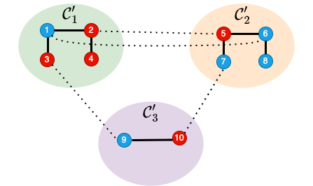
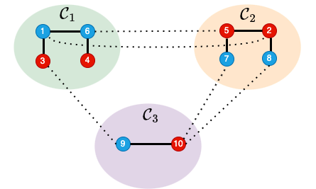
Let $p=10$, $H=2$, $\mathcal{D}_{1}=\{1,6,7,8,9\}$, and $\mathcal{D}_{2}=\{2,3,4,5,10\}$. This gives the group membership matrix as follows:

$${\bf{R}}=\begin{bmatrix}1&0&0&0&0&1&1&1&1&0\\ 0&1&1&1&1&0&0&0&0&1\\ 0&1&1&1&1&0&0&0&0&1\\ 0&1&1&1&1&0&0&0&0&1\\ 0&1&1&1&1&0&0&0&0&1\\ 1&0&0&0&0&1&1&1&1&0\\ 1&0&0&0&0&1&1&1&1&0\\ 1&0&0&0&0&1&1&1&1&0\\ 1&0&0&0&0&1&1&1&1&0\\ 0&1&1&1&1&0&0&0&0&1\end{bmatrix}.$$

Set $K=3$. Define $\mathcal{C}_{1}^{\prime}=\{1,2,3,4\}$, $\mathcal{C}_{2}^{\prime}=\{5,6,7,8\}$, $\mathcal{C}_{3}^{\prime}=\{9,10\}$, $\mathcal{C}_{1}=\{1,3,4,6\}$, $\mathcal{C}_{2}=\{2,5,7,8\}$, $\mathcal{C}_{3}^{\prime}=\{9,10\}$. ${\bf{Q}}^{\prime}$ and ${\bf{Q}}$ provide the membership matrices associated with clusterings $\mathcal{C}_{1}^{\prime}\cup\mathcal{C}_{2}^{\prime}\cup\mathcal{C}_{3}^{\prime}$ and $\mathcal{C}_{1}\cup\mathcal{C}_{2}\cup\mathcal{C}_{3}$, respectively, as follow:

$${\bf{Q}}^{\prime} =\begin{bmatrix}\frac{1}{4}&\frac{1}{4}&\frac{1}{4}&\frac{1}{4}&0&0&0&0&0&0\\ \frac{1}{4}&\frac{1}{4}&\frac{1}{4}&\frac{1}{4}&0&0&0&0&0&0\\ \frac{1}{4}&\frac{1}{4}&\frac{1}{4}&\frac{1}{4}&0&0&0&0&0&0\\ \frac{1}{4}&\frac{1}{4}&\frac{1}{4}&\frac{1}{4}&0&0&0&0&0&0\\ 0&0&0&0&\frac{1}{4}&\frac{1}{4}&\frac{1}{4}&\frac{1}{4}&0&0\\ 0&0&0&0&\frac{1}{4}&\frac{1}{4}&\frac{1}{4}&\frac{1}{4}&0&0\\ 0&0&0&0&\frac{1}{4}&\frac{1}{4}&\frac{1}{4}&\frac{1}{4}&0&0\\ 0&0&0&0&\frac{1}{4}&\frac{1}{4}&\frac{1}{4}&\frac{1}{4}&0&0\\ 0&0&0&0&0&0&0&0&\frac{1}{2}&\frac{1}{2}\\ 0&0&0&0&0&0&0&0&\frac{1}{2}&\frac{1}{2}\\ \end{bmatrix},$$

$$~{}~{}~{}~{}{\bf{Q}} =\begin{bmatrix}\frac{1}{4}&0&\frac{1}{4}&\frac{1}{4}&0&\frac{1}{4}&0&0&0&0\\ 0&\frac{1}{4}&0&0&\frac{1}{4}&0&\frac{1}{4}&1&0&0\\ \frac{1}{4}&0&\frac{1}{4}&\frac{1}{4}&0&\frac{1}{4}&0&0&0&0\\ \frac{1}{4}&0&\frac{1}{4}&\frac{1}{4}&0&\frac{1}{4}&0&0&0&0\\ 0&\frac{1}{4}&0&0&\frac{1}{4}&0&\frac{1}{4}&\frac{1}{4}&0&0\\ \frac{1}{4}&0&\frac{1}{4}&\frac{1}{4}&0&\frac{1}{4}&0&0&0&0\\ 0&\frac{1}{4}&0&0&\frac{1}{4}&0&\frac{1}{4}&\frac{1}{4}&0&0\\ 0&\frac{1}{4}&0&0&\frac{1}{4}&0&\frac{1}{4}&\frac{1}{4}&0&0\\ 0&0&0&0&0&0&0&0&\frac{1}{2}&\frac{1}{2}\\ 0&0&0&0&0&0&0&0&\frac{1}{2}&\frac{1}{2}\end{bmatrix}.\qquad\qquad\qquad\qquad$$

For each $h\in\{1,2\}$, we get:

$$\frac{|\mathcal{D}_{h}\cap\mathcal{C}_{k}^{\prime}|}{|\mathcal{C}_{k}^{\prime}|} \neq\frac{|\mathcal{D}_{h}|}{p}=\frac{1}{2}~{}~{}\text{for some}~{}~{}k\in\{1,2,3\}~{}~{}~{}\text{and}~{}~{}~{}{\bf{R}}({\bf{I}}-{\bf{J}}_{p}/p){\bf{Q}}^{\prime}\neq{\bf{0}},$$

$$\frac{|\mathcal{D}_{h}\cap\mathcal{C}_{k}|}{|\mathcal{C}_{k}|} =\frac{|\mathcal{D}_{h}|}{p}=\frac{1}{2}~{}~{}\text{for all}~{}~{}k\in\{1,2,3\}~{}~{}~{}\text{and}~{}~{}~{}{\bf{R}}({\bf{I}}-{\bf{J}}_{p}/p){\bf{Q}}={\bf{0}}.$$

Hence, ${\bf{Q}}$ is a fair partition matrix (clustering). Figures 1 (left) and (right) show the graphical models generated with probabilities (39) and using the membership matrices ${\bf{Q}}^{\prime}$ and ${\bf{Q}}$, respectively.

4.4 Comparison to Community Detection Methods in the Known Graph Setting

In this section, we consider the graph structure to be known. Specifically, we assume that the graph matrix $\Theta$ is constructed following the procedure outlined in the first step of data generation, as detailed in Section 4.3.

To evaluate our methods, we compare them against the following baselines in the context of convex community detection:

1. Two-stage approach for which we (ii) apply a community detection approach [8] to compute partition matrix $\hat{{\bf{Q}}}$, and (ii) employ a K-means clustering to obtain clusters.

2. Two-stage approach for which we (ii) apply a community detection approach [17] to compute partition matrix $\hat{{\bf{Q}}}$, and (ii) employ a K-means clustering to obtain clusters.

FCD. Two-stage approach for which we (ii) apply the fair community detection approach in (17) to compute partition matrix $\hat{{\bf{Q}}}$, and (ii) employ a K-means clustering to obtain clusters.

Figure 3: CE and runtime (in seconds) of CD-I, CD-II [17], and FCD of an SBM with $H=5$, $K=5$.

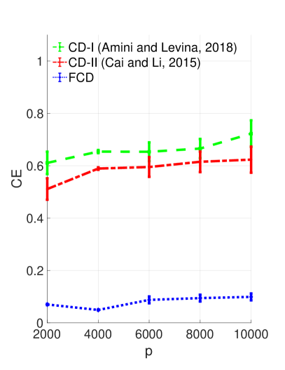
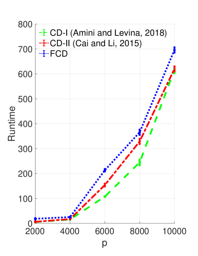
Figure 3 presents the CE and runtime (in seconds) from repeating the procedure 10 times for the CD-I, CD-II [17], and FCD methods on an SBM with $H=5$, $K=5$. We observe that the FCD method demonstrates significantly lower clustering error compared to both CD-I [8] and CD-II [17]. Furthermore, CD-I and CD-II yield comparable results in terms of clustering error, with CD-II showing a marginally better performance. Additionally, despite incorporating an extra fairness constraint, FCD’s runtime is comparable to the other methods, indicating that the inclusion of this constraint does not adversely affect its computational efficiency.

4.5 Comparison to Graphical Lasso and Neighbourhood Selection Methods in the unknown Graph Setting

We consider four setups for comparing our methods with community-based graphical models (GM):

1. Three-stage approach for which we (i) use a GM to estimate precision matrix $\hat{\mbox{\boldmath$\Theta$}}$, (ii) apply a community detection approach [17] to compute partition matrix $\hat{{\bf{Q}}}$, and (iii) employ a K-means clustering to obtain clusters.

2. Two-stage approach for which we (i) use (12) without fairness constraint to simultaneously estimate precision and partition matrices and (ii) employ a K-means clustering to obtain clusters.

1. Three-stage approach for which we (i) use a GM to estimate precision matrix $\hat{\mbox{\boldmath$\Theta$}}$, (ii) apply a community detection approach [17] to compute partition matrix $\hat{{\bf{Q}}}$, and (iii) employ a fair K-means clustering [29] to obtain clusters.

2. Two-stage approach for which we (i) use (12) to simultaneously estimate precision and partition matrices and (ii) employ the K-means clustering to obtain clusters.

The main goal of Setups I. and II. is to compare the community detection errors without fairness constraints under different settings of $L$ and $G$ functions.

We consider three type of GMs in Setups I.–FII.:

1. A graphical Lasso-type method [38] implemented using the objective with $L(\mbox{\boldmath$\Theta$};{\bf{Y}})=n/2[-\log\det(\mbox{\boldmath$\Theta$})+\operatorname{trace}({\bf{S}}\mbox{\boldmath$\Theta$})]$ and $G(\mbox{\boldmath$\Theta$})=\mbox{\boldmath$\Theta$}$.

2. A neighborhood selection-type method [58] implemented using $L(\mbox{\boldmath$\Theta$};{\bf{Y}})=n/2[-\log|\text{diag}(\mbox{\boldmath$\Theta$}^{2})|+\text{trace}({\bf{S}}\mbox{\boldmath$\Theta$}^{2})]$ and $G(\mbox{\boldmath$\Theta$})=\mbox{\boldmath$\Theta$}^{2}$.

3. A neighborhood selection-type method [89] implemented using $L(\mbox{\boldmath$\Theta$};{\bf{Y}})=-\sum_{j=1}^{p}\sum_{j^{\prime}=1}^{p}\theta_{jj^{\prime}}s_{jj^{\prime}}+1/n\sum_{i=1}^{n}\sum_{j=1}^{p}\log\big{(}1+\exp(\theta_{jj}+\sum_{j^{\prime}\neq j}\theta_{jj^{\prime}}y_{ij^{\prime}})\big{)}$ and $G(\mbox{\boldmath$\Theta$})=\mbox{\boldmath$\Theta$}$.

In our results, we name each one “GM-Type-Setup” to refer to the GM type and the setup above. For example, GM-A.II. refers to a graphical Lasso used in the first step of the two stage approach in II. It is worth mentioning that GM-A.II. and GM-B.FI. can be seen as variants of the cluster-based GLASSO [88, 64, 54] and fair K-means applied to spectral clustering [59], respectively. Note that unlike [59], which assume that the graph structure and the number of communities are given in advance, GM-B.FI. learns fair community structure while estimating heterogeneous GMs.

Sample Size	Method	CE	PCEE
$n=300$	GM-B.I.	0.464(0.015)	0.773(0.010)
	GM-B.II.	0.426(0.015)	0.791(0.010)
	GM-B.FI.	0.197(0.005)	0.773(0.010)
	GM-B.FII.(FCONCORD)	0.060(0.005)	0.835(0.010)
$n=450$	GM-B.I.	0.423(0.015)	0.813(0.010)
	GM-B.II.	0.418(0.011)	0.863(0.010)
	GM-B.FI.	0.163(0.015)	0.813(0.010)
	GM-B.FII.(FCONCORD)	0.011(0.005)	0.891(0.012)

Table 1: Simulation results of neighborhood selection-type GMs on SBM network. The results are for $p=600$, $H=3$, and $K=2$.

We repeated the procedure 10 times and reported the averaged clustering errors and proportion of correctly estimated edges. Tables 1 and 2 is for SBM with $p=300$. As shown in Tables 1 and 2, GM-A.I., GM-A.II., GM-B.I., and GM-B.I. have the largest clustering error and the proportion of correctly estimated edges. GM-A.II. and GM-B.II. improve the performance of GM-A.I. and GM-B.I. in the precision matrix estimation. However, they still incur a relatively large clustering error since they ignore the similarity across different community matrices and employ a standard K-means clustering. In contrast, our FCONCORD and FGLASSO algorithms achieve the best clustering accuracy and estimation accuracy for both scenarios. This is due to our simultaneous clustering and estimation strategy as well as the consideration of the fairness of precision matrices across clusters. This experiment shows that a satisfactory fair community detection algorithm is critical to achieve accurate estimations of heterogeneous and fair GMs, and alternatively good estimation of GMs can also improve the fair community detection performance. This explains the success of our simultaneous method in terms of both fair clustering and GM estimation.

Sample Size	Method	CE	PCEE
$n=300$	GM-A.I.	0.431(0.015)	0.731(0.011)
	GM-A.II.	0.416(0.015)	0.761(0.011)
	GM-A.FI.	0.182(0.006)	0.731(0.011)
	GM-A.FII. (FGLASSO)	0.097(0.006)	0.815(0.050)
$n=450$	GM-A.I.	0.470(0.011)	0.792(0.010)
	GM-A.II.	0.406(0.011)	0.803(0.010)
	GM-A.FI.	0.163(0.005)	0.792(0.010)
	GM-A.FII.(FGLASSO)	0.050(0.005)	0.863(0.012)

Table 2: Simulation results of graphical Lasso-type algorithms on SBM network. The results are for $p=600$, $H=3$, and $K=2$.

Sample Size	Method	CE	PCEE
$n=200$	GM-C.I.	0.489(0.011)	0.601(0.010)
	GM-C.II.	0.461(0.005)	0.651(0.010)
	GM-C.FI.	0.219(0.005)	0.601(0.010)
	GM-C.FII.(FBN)	0.117(0.009)	0.738(0.005)
$n=400$	GM-C.I.	0.434(0.010)	0.637(0.010)
	GM-C.II.	0.461(0.010)	0.681(0.010)
	GM-C.FI.	0.219(0.005)	0.637(0.010)
	GM-C.FII.(FBN)	0.104(0.005)	0.796(0.005)

Table 3: Simulation results of binary neighborhood selection-type GMs on SIBM network. The results are for $p=100$, $H=2$, and $K=2$.

Next, we consider a natural composition of SBM and the Ising model called Stochastic Ising Block Model (SIBM); see, e.g., [13, 110] for more details. In SIBM, we take SBM similar to (39), where $p$ vertices are divided into clusters and subgroups and the edges are connected independently with probability $\{\xi_{i}\}_{i=1}^{4}$. Then, we use the graph $\mathcal{G}$ generated by the SBM as the underlying graph of the Ising model and draw $n$ i.i.d. samples from it. The objective is to exactly recover the fair clusters in SIBM from the samples generated by the Ising model, without observing the graph $\mathcal{G}$.

Tables 3 reports the averaged clustering errors and the proportion of correctly estimated edges for SIBM with $p=100$. The standard GM-C.I. method has the largest clustering error due to its ignorance of the network structure in the precision matrices. GM-C.FI. improves the clustering performance of the GM-C.I. by using the method of [89] in the precision matrix estimation and the robust community detection approach [17] for computing partition matrix $\hat{{\bf{Q}}}$. GM-C.FII. is able to achieve the best clustering performance due to the procedure of simultaneous fair clustering and heterogeneous GMs estimation.

5 Real Data Application

5.1 Application to Friendship Network

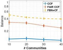
In this experiment, we assume the network matrix $\Theta$ is given a priori. In the experiments of Figure 4, we evaluate the performance of standard semidefinite programming as in [17] versus our fair versions on real network data. The quality of a clustering is measured through its “Balance” defined in (38) and runtime. Figure 4 shows the results as a function of the number of clusters $k$ for two high school friendship networks [75]. Vertices correspond to students and are split into two groups of males and females ($H=2$). Friendship network has 127 vertices, and an edge between two students indicates that one of them reported friendship with the other one. The network is the largest connected component of an originally unconnected network.

Figure 4: Balance and runtime (in seconds) of CD-I, CD-II [17], and FCD on Friendship Network as a function of the number $k$ of clusters.

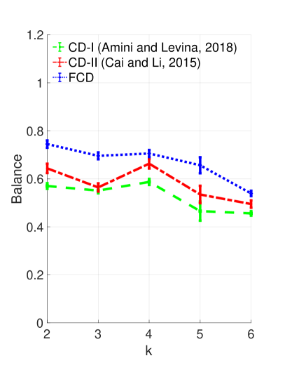
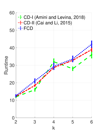
In Figure 4, we observe that FCD demonstrates enhanced fairness compared to both CD-I [8] and CD-II [17] in terms of balance. Moreover, CD-I and CD-II yield comparable results in terms of balance, with CD-II exhibiting marginally better balance. Additionally, despite incorporating an additional fairness constraint, the runtime of FCD is not significantly worse than the other methods.

5.2 Application to Word Embeddings

Word embeddings are a form of word representation in an $p$-dimensional space. Word embeddings serve as a dictionary of sorts for computer programs that uses word meaning. The rationale behind word embeddings is that words with similar semantic meanings tend to have representations that are close together in the vector space than dissimilar words. This makes word embeddings useful by allowing them to represent the relationship between words in mathematical terms, making them an important and widely used component in many Natural Language Processing (NLP) models. However, despite its expansive applications, word embeddings have been found to exhibit strong, ethically questionable biases such as a bias against a specific race, gender, religion, and sexual preferences among others [14, 20, 86].

GMs are widely used in word embedding applications where the goal is to understand the relationships among the words/terms and their community structures [97, 51]. In the following, we focus on the issues and the improvement of the GM approaches we have towards detecting and dealing with bias in word embeddings. To do so, we evaluated the bias based on data obtained from the preprocessed English dataset of the Small World of Words [33]. The goal of the analysis is to understand the relationships among the cue terms, identify cue words that are hubs, and correct the bias in their community structure. This dataset contains the responses of 83,864 participants in a word association task to 12,292 cue words. Each cue word was judged by exactly 100 participants; see Table 4.

In our implementation, cue words and the responses from participants are considered random variables and the samples for the estimation of GMs, respectively. We apply a tokenizer to transform text data into numerical values (using Word2Vec algorithm). We select the 250 cue words for our numerical evaluations as follows: we first select 10 cue words uniformly at random and then select 25 words with the highest similarity to each cue word following [33]. We manually assign gender for each cue term. For example, the cue word “woman” (a node in GM) is female (group $\#1$), the cue word “man” is male (group $\#2$), and the cue word “doctor” can be both female and man (groups $\#1$ and 2). Please refer to Table 4 for further descriptions.

Participant Age Gender Native Country Cue R1 R2 R3 Cue ID Language Group ($h$) 376 38 Fe Australia Australia strong box man weak 1 and 2 1062 19 Ma Australia Australia sick ill hospital disease 1 and 2 4295 77 Ma US US doctor nurse professor physician 1 and 2 4136 44 Ma UK Spain mother woman hair emotions 1 4214 63 Fe US US man woman boy child 2

Table 4: The data collected as part of the Small World of Words dataset. Each participant gave 3 responses (R1, R2, R3) to each cue word that they were presented with. The last column shows our manual group assignments.

	Method	RCut	Balance
$K=5$	GM-B.II.	9.4 (0.1)	0.324 (0.005)
	GM-B.FII.(FCONCORD)	8.7 (0.1)	0.439 (0.005)
$K=10$	GM-B.II.	15.1 (0.1)	0.507 (0.005)
	GM-B.FII.(FCONCORD)	14.9 (0.1)	0.619 (0.005)

Table 5: The ratio cut and balance of various methods in the Word Embedding data set.

Figure 5: Subgraphs of the precision matrices estimated by GM-B.II.(left) and GM-B.FII.(right). Nodes represent the cue labeled by their word. Circle markers denote words within a healthcare community, and square markers denote isolated words. The width of a link is proportional to the magnitude of the corresponding partial correlations. GM-B.FII.(FCONCORD) enhances the neutrality from gender bias and improves the related word connection within the healthcare community.

Despite the adoption of different graph learning algorithms for this dataset, the existing methods often do not have fairness considerations. Although one may manually remove the protected attributes in the selected features to avoid discrimination, a number of non-protected attributes that are highly correlated with the protected attributes may still be selected by these methods and result in discrimination. To address this issue, we next implement the proposed FCONCORD which uses a joint $\ell_{1}$–regularized regressions for each node (cue word) of a graph associated with the feature covariance matrix with tuning parameters selected using (4.1).

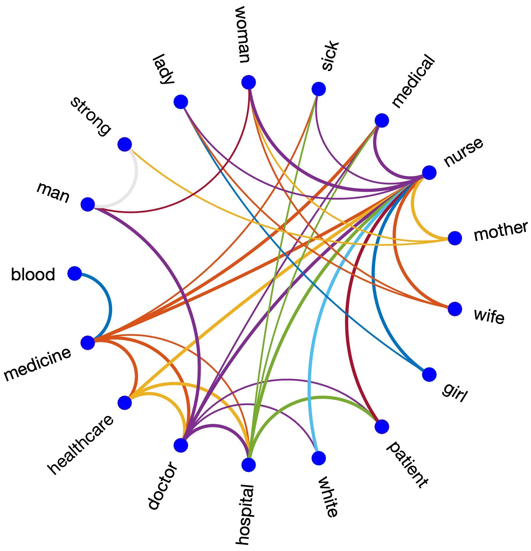
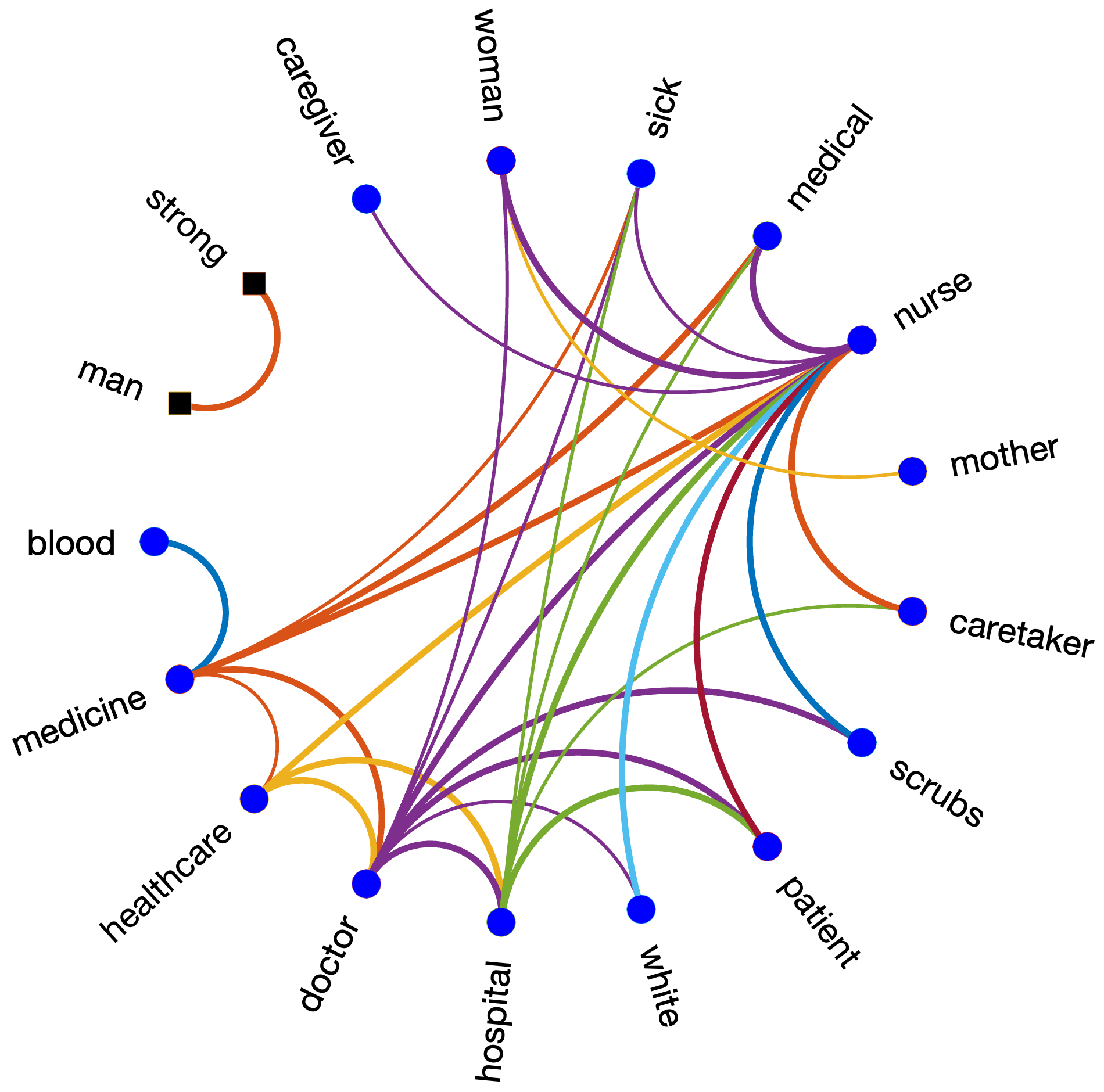
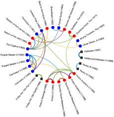
Table 5 compares various algorithms in terms of Ratio Cut (RCut) and Balance. Not only FCONCORD is able to achieve a higher balance, but it also does so with a better RCut as compared to GM-B.II.. In addition, the estimated communities for two sub-graphs of cue words are also shown in Figure 5. From both networks, we can see that the estimated communities mainly consist of healthcare communities. The estimated network also shows two hub nodes: “doctor ”and “nurse ”. For instance, the fact that the nurse is a hub indicates that many term occurrences (in the medical community) are explained by the occurrence of the word nurse. These results provide an intuitive explanation of the relationships among the terms in the cue word communities. We also note that FCONCORD enhances the neutrality from gender bias by removing the connection between biased edges such as (lady, nurse), (girl, nurse), and (doctor, man).

5.3 Application to Fair Community Detection in Recommender System

Recommender systems (RS) model user-item interactions to provide personalized item recommendations that will suit the user’s taste. Broadly speaking, two types of methods are used in such systems—content based and collaborative filtering. Content based approaches model interactions through user and item covariates. Collaborative filtering (CF), on the other hand, refers to a set of techniques that model user-item interactions based on user’s past response.

A popular class of methods in RS is based on clustering users and items [102, 83, 93, 94]. Indeed, it is more natural to model the users and the items using clusters (communities), where each cluster includes a set of like-minded users or the subset of items that they are interested in. The overall procedure of this method, called cluster CF (CCF), contains two main steps. First, it finds clusters of users and/or items, where each cluster includes a group of like-minded users or a set of items that these users are particularly interested in. Second, in each cluster, it applies traditional CF methods to learn users’ preferences over the items within this cluster. Despite efficiency and scalability of these methods, in many human-centric applications, using CCF in its original form can result in unfavorable and even harmful clustering and prediction outcomes towards some demographic groups in the data.

It is shown in [94, 80] that using item-item similarities based on “who-rated-what” information is strongly correlated with how users explicitly rate items. Hence, using this information as user covariates helps in improving predictions for explicit ratings. Further, one can derive an item graph where edge weights represent movie similarities that are based on global “who-rated-what” matrix [61, 104, 2, 77]. Imposing sparsity on such a graph and finding its fair communities is attractive since it is intuitive that an item is generally related to only a few other items. This can be achieved through our fair GMs. Such a graph gives a fair neighborhood structure that can also help better predict explicit ratings. In addition to providing useful information to predict ratings, we note that using who-rated-what information also provides information to study the fair relationships among items based on user ratings.

The goal of our analysis is to understand the balance and prediction accuracy of fair GMs on RS datasets as well as the relationships among the items in these datasets. We compare the performance of our fair GMs implemented in the framework of standard CCF and its fair K-means variant. In particular, we consider the following algorithms:

• FGLASSO (FCONCORD)+CF: A two-stage approach for which we first use FGLASSO (FCONCORD) to obtain the fair clusters and then apply traditional CF to learn users’ preferences over the items within each cluster. We set $\rho_{1}=1$, $\rho_{2}=0.05$, $\gamma=0.01$, and $\epsilon=1e-3$ in our implementations.

• CCF (Fair CCF): A two-stage approach for which we first use K-means (fair K-means [29]) clustering to obtain the clusters and then apply CF to learn users’ preferences within each cluster [102].

5.3.1 Music Data

Music RSs are designed to give personalized recommendations of songs, playlists, or artists to a user, thereby reflecting and further complementing individual users’ specific music preferences. Although accuracy metrics have been widely applied to evaluate recommendations in music RS literature, evaluating a user’s music utility from other impact-oriented perspectives, including their potential for discrimination, is still a novel evaluation practice in the music RS literature [36, 24, 95]. Next, we center our attention on artists’ gender bias for which we want to estimate if standard music RSs may exacerbate its impact.

Figure 6: Input Preference Ratio (PR) distributions of LFM-360K dataset.

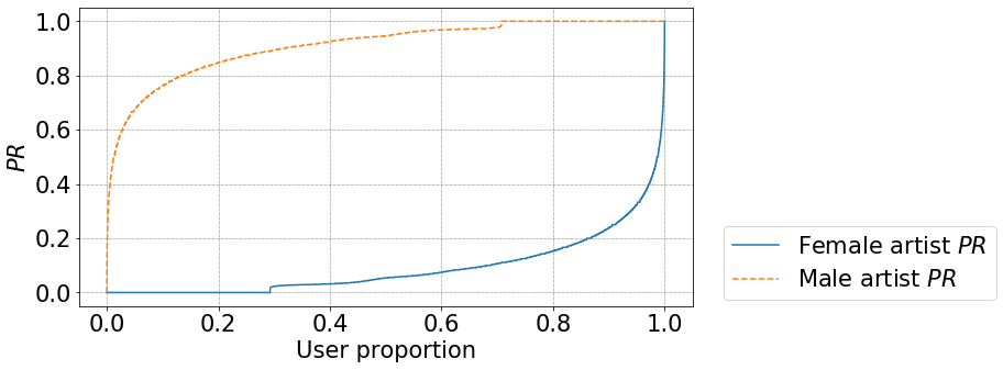
To illustrate the impact of artists gender bias in RSs, we use the freely available binary LFM-360K music dataset. The LFM-360K consists of approximately 360,000 users listening histories from Last.fm collected during Fall 2008. We generate recommendations for a sample of all users for which gender can be identified. We limit the size of this sample to be 10% randomly chosen of all male and female users in the whole dataset due to computational constraints. Let $\mathcal{U}$ be the set of $n$ users, $\mathcal{I}$ be the set of $p$ items and ${\bf{Y}}$ be the $n\times p$ input matrix, where $y_{ui}=1$ if user $u$ has selected item $i$, and zero otherwise. Given the matrix ${\bf{Y}}$, the input preference ratio (PR) for user group $\mathcal{D}$ on item category $\mathcal{C}$ is the fraction of liked items by group $\mathcal{D}$ in category $\mathcal{C}$, defined as the following [95]:

$$\textnormal{PR}(\mathcal{D},\mathcal{C}):=\frac{\sum_{u\in\mathcal{D}}\sum_{i\in\mathcal{C}}y_{ui}}{\sum_{u\in\mathcal{D}}\sum_{i\in\mathcal{I}}y_{ui}}.$$ (40)

Figure 6 represents the distributions of users’ input PR towards male and female artist groups. It shows that only around 20% of users have a PR towards male artists lower than 0.8. On the contrary, 80% of users have a PR lower than 0.2 towards female artists. This shows that commonly deployed state of the art CF algorithms may act to further increase or decrease artist gender bias in user-artist RS.

Figure 7: RMSE (left) and Balance (right) of standard CCF, Fair CCF, and FBN+CF on LFM-360K music data.

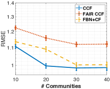
Next, we study the balance and prediction accuracy of fair GMs on music RSs. Figure 7 indicates that the proposed FBN+CF has the best performance in terms of the balance and root mean squared error (RMSE). As expected, the baseline with no notion of fairness–CCF–results in the best overall precision. Of the two fairness-aware approaches, the fair K-means-based approach–Fair CCF–performs considerably below FBN+CF. This suggests that recommendation quality can be preserved, but leaves open the question of whether we can improve fairness. Hence, we turn to the impact on the fairness of the three approaches. Figure 7(right) presents the balance. We can see that fairness-aware approaches–Fair CCF and FBN+CF–have a strong impact on the balance in comparison with standard CCF. And for RMSE, we see that FBN+CF achieves a much better rating difference in comparison with Fair CCF, indicating that we can induce aggregate statistics that are fair between the two sides of the sensitive attribute (male vs. female).

5.3.2 MovieLens Data

We use the MovieLens 10K dataset. Following previous works [60, 56, 24], we use year of the movie as a sensitive attribute and consider movies before 1991 as old movies. Those more recent are considered new movies. [60] showed that the older movies have a tendency to be rated higher, perhaps because only masterpieces have survived. When adopting year as a sensitive attribute, we show that our fair graph-based RS enhances the neutrality from this masterpiece bias. The clustering balance and RMSE have been used to evaluate different modeling methods on this dataset. Since reducing RMSE is the goal, statistical models assume the response (ratings) to be Gaussian for this data [61, 104, 2].

Figure 8: RMSE (left) and Balance (right) of standard CCF, Fair CCF, FGLASSO+CF, and FCONCORD+CF on MovieLens 10K data.

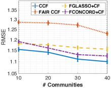
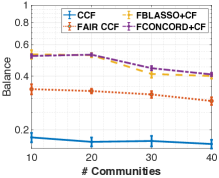
Experimental results are shown in Figure 8. As expected, the baseline with no notion of fairness–CCF–results in the best overall RMSEs, with our two approaches (FGLASSO+CF and FCONCORD+CF) providing performance fairly close to CCF. Figure 8 (right) shows that compared to fair CCF, FGLASSO+CF and FCONCORD+CF significantly improve the clustering balance. Hence, our fair graph-based RSs successfully enhanced the neutrality without seriously sacrificing the prediction accuracy.

GM-B.II. The pair of movies Partial correlation The Godfather (1972) The Godfather: Part II (1974) 0.592 Grumpy Old Men (1993) Grumpier Old Men (1995) 0.514 Patriot Games (1992) Clear and Present Danger (1994) 0.484 The Wrong Trousers (1993) A Close Shave (1995) 0.448 Toy Story (1995) Toy Story 2 (1999) 0.431 Star Wars: Episode IV–A New Hope (1977) Star Wars: Episode V–The Empire Strikes Back (1980) 0.415 GM-B.FII. (FCONCORD) The pair of movies Partial correlation The Godfather (1972) The Godfather: Part II (1974) 0.534 Grumpy Old Men (1993) Grumpier Old Men (1995) 0.520 Austin Powers: International Man of Mystery (1997) Austin Powers: The Spy Who Shagged Me (1999) 0.491 Toy Story (1995) Toy Story 2 (1999) 0.475 Patriot Games (1992) Clear and Present Danger (1994) 0.472 The Wrong Trousers (1993) A Close Shave (1995) 0.453

Table 6: Pairs of movies with top 5 absolute values of partial correlations in the precision matrix from GM-B.II. and GM-B.FII.(FCONCORD).

Fair GMs also provide information to study the relationships among items based on user ratings. To illustrate this, the top-5 movie pairs with the highest absolute values of partial correlations are shown in Table 6. If we look for the highly related movies to a specific movie in the precision matrix, we find that FCONCORD enhances the balance by assigning higher correlations to more recent movies such as “The Wrong Trousers” (1993) and “A Close Shave” (1995).

Figure 9: Subgraphs of the precision matrices estimated by GM-B.II.(left) and GM-B.FII.(right). Nodes represent the movies labeled by their titles. Circle markers denote movies within a single community in each subgraph, and square markers denote isolated movies. Blue nodes are new movies and red nodes old movies within each community. The width of a link is proportional to the magnitude of the corresponding partial correlations. GM-B.FII.(FCONCORD) enhances the neutrality from year bias by replacing the old movies within each community by new ones.

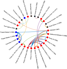
In addition, the estimated communities for two sub-graphs of movies are also shown in Figure 9. From both networks, we can see that the estimated communities mainly consist of mass-marketed commercial movies, dominated by action films. Note that these movies are usually characterized by high production budgets, state-of-the-art visual effects, and famous directors and actors. Examples in this community include “The Godfather (1972) ”, “Terminator 2 (1991) ”, and “Return of the Jedi (1983)”, “Raiders of Lost Ark (1981)”, etc. As expected, movies within the same series are most strongly associated. Figure 9 (right) shows that FCONCORD enhances the neutrality from the old movies bias by replacing them with new ones such as “Jurassic Park (1993)”, “The Wrong Trousers(1993) ”, and “A Close Shave (1995)”.

6 Conclusion

In this work, we developed a novel approach to learning fair graphical models with community structure. Our goal is to motivate a new line of work for fair community learning in graphical models that can begin to alleviate fairness concerns in this important subtopic within unsupervised learning. We established statistical consistency of the proposed method for both a Gaussian GM and an Ising model proving that our method can recover the graphs and their fair communities with high probability. We applied the proposed framework to the tasks of estimating a Gaussian graphical model and a binary network. The proposed framework can also be applied to other types of graphical models, such as the Poisson graphical model [4] or the exponential family graphical model [109].

Appendix

The appendix is organized as follows:

• Appendix 6.1 provides some preliminaries used in the proof of main theorems.

• Appendix 6.2 provides large sample properties of FCONCORD, i.e., the proof of Theorem 5.

• Appendix 6.3 provides large sample properties of FBN, i.e., the proof of Theorem 6.

• Appendix 6.4 gives the consistency of fair community labeling in graphical models.

• Appendix 6.5 provides the detailed derivation of the updates for Algorithm 1.

6.1 Preliminaries

Let $F(\mbox{\boldmath$\Theta$},{\bf{Q}};{\bf{Y}})=n/2\big{[}-\log|\text{diag}(\mbox{\boldmath$\Theta$})^{2}|+\operatorname{trace}\big{(}({\bf{S}}+\rho_{2}{\bf{Q}})\mbox{\boldmath$\Theta$}^{2}\big{)}\big{]}$. Let the notation ${F}_{n}(\mbox{\boldmath$\theta$}^{d},\mbox{\boldmath$\theta$}^{o},{\bf{q}}^{d},{\bf{q}}^{o};{\bf{Y}})$ stands for $\frac{{F}}{n}$. We introduce a restricted version of criterion (3.1) as below:

$$\operatorname*{minimize}_{\mbox{\boldmath$\theta$}^{o},\mbox{\boldmath$q$}^{o}}~{}~{}F_{n}(\bar{\mbox{\boldmath$\theta$}}^{d},\mbox{\boldmath$\theta$}^{o},\bar{{\bf{q}}}^{d},{\bf{q}}^{o};{\bf{Y}})+\rho_{1n}\|\mbox{\boldmath$\theta$}^{o}\|_{1},~{}~{}~{}\text{subj. to}~{}~{}\mbox{\boldmath$\theta$}^{o}_{\mathcal{B}^{c}}=0.$$ (41)

We define a linear operator $\mathcal{A}:{\mathbb{R}}^{p(p-1)/2}\rightarrow{\mathbb{R}}^{p\times p}$, ${\bf{w}}\rightarrow\mathcal{A}{\bf{w}}$, satisfying

$$[\mathcal{A}{\bf{w}}]_{ij}=\begin{cases}-w_{i+d_{j}}\;&\;\;i>j,\\ [\mathcal{A}{\bf{w}}]_{ji}\;&\;\;i<j,\\ 0\;&\;\;i=j,\end{cases}$$ (42)

where $d_{j}=-j+\frac{j-1}{2}(2p-j).$ An example for $\mathcal{A}{\bf{w}}$ on ${\bf{w}}=[w_{1},w_{2},\cdots,w_{6}]^{\top}$ is given below

$$\mathcal{A}{\bf{w}}=\left[\begin{array}[]{cccc}0&w_{1}&w_{2}&w_{3}\\ w_{1}&0&w_{4}&w_{5}\\ w_{2}&w_{4}&0&w_{6}\\ w_{3}&w_{5}&w_{6}&0\end{array}\right].$$

We derive the adjoint operator $\mathcal{A}^{*}$ of $\mathcal{A}$ by making $\mathcal{A}^{*}$ satisfy $\langle\mathcal{A}{\bf{w}},{\bf{z}}\rangle=\langle{\bf{w}},\mathcal{A}^{*}{\bf{z}}\rangle$; see, [64, Section 4.1] for more details.

Let ${\bf{Q}}^{o}=\text{diag}(\bar{{\bf{q}}}^{d})+\mathcal{A}{\bf{q}}^{o}$ and $\mbox{\boldmath$\Theta$}^{o}=\text{diag}(\bar{\mbox{\boldmath$\theta$}}^{d})+\mathcal{A}\mbox{\boldmath$\theta$}^{o}$. Since by our assumption $\mbox{\boldmath$\epsilon$}={\bf{0}}$, we obtain

$$~{}\begin{array}[]{ll}\underset{\mbox{\boldmath$\theta$}^{o},\mbox{\boldmath$q$}^{o}}{\text{minimize}}&\begin{array}[]{c}\hskip 14.22636ptL_{n}(\bar{\mbox{\boldmath$\theta$}}^{d},\mbox{\boldmath$\theta$}^{o};{\bf{Y}})+\rho_{1n}\|\mbox{\boldmath$\theta$}^{o}\|_{1}+\rho_{2n}\operatorname{trace}(\mbox{\boldmath$\Theta$}^{o}{\bf{Q}}^{o}\mbox{\boldmath$\Theta$}^{o}),\end{array}\\ \text{subj. to}&\begin{array}[t]{l}\hskip 14.22636pt\mbox{\boldmath$\theta$}^{o}_{\mathcal{B}^{c}}=0,~{}~{}{\bf{Q}}^{o}\succeq{\bf{0}},~{}~{}{\bf{A}}_{1}{\bf{Q}}^{o}={\bf{0}},~{}~{}{\bf{0}}\leq{\bf{Q}}^{o}\leq{\bf{J}}_{p}.\end{array}\end{array}$$ (47)

It is easy to see that $\textnormal{rank}({\bf{A}}_{1})=H-1$. Let ${\bf{N}}\in{\mathbb{R}}^{p\times(p-H+1)}$ be a matrix whose rows form an orthonormal basis of the nullspace of ${\bf{A}}_{1}$. We can substitute ${\bf{Q}}^{o}={\bf{N}}{\bf{R}}^{o}{\bf{N}}^{\top}$ for ${\bf{R}}^{o}\in{\mathbb{R}}^{(p-H+1)\times(p-H+1)}$, and then, using that ${\bf{N}}^{\top}{\bf{N}}={\bf{I}}_{(p-H+1)}$, Problem (47) becomes

$$~{}\begin{array}[]{ll}\underset{\mbox{\boldmath$\theta$}^{o},\mbox{\boldmath$r$}^{o}}{\text{minimize}}&\begin{array}[]{c}\hskip 14.22636ptF_{n}(\bar{\mbox{\boldmath$\theta$}}^{d},\mbox{\boldmath$\theta$}^{o},\bar{{\bf{r}}}^{d},{\bf{r}}^{o};{\bf{Y}})+\rho_{1n}\|\mbox{\boldmath$\theta$}^{o}\|_{1}\end{array}\\ \text{subj. to}&\begin{array}[t]{l}\hskip 14.22636pt\mbox{\boldmath$\theta$}^{o}_{\mathcal{B}^{c}}=0,~{}~{}{\bf{Q}}^{o}\succeq{\bf{0}},~{}~{}{\bf{0}}\leq{\bf{Q}}^{o}\leq{\bf{J}}_{p},\end{array}\end{array}$$ (52)

where $F_{n}(\bar{\mbox{\boldmath$\theta$}}^{d},\mbox{\boldmath$\theta$}^{o},\bar{{\bf{r}}}^{d},{\bf{r}}^{o};{\bf{Y}})=L_{n}(\bar{\mbox{\boldmath$\theta$}}^{d},\mbox{\boldmath$\theta$}^{o};{\bf{Y}})+\rho_{2n}\operatorname{trace}(\mbox{\boldmath$\Theta$}^{o}{\bf{N}}{\bf{R}}^{o}{\bf{N}}^{\top}\mbox{\boldmath$\Theta$}^{o})$.

Throughout, we use $\bar{{\bf{g}}}^{n}$ and $\bar{{\bf{H}}}^{n}$ to denote the gradient and the Hessian of $L_{n}(\bar{\mbox{\boldmath$\theta$}}^{d},\mbox{\boldmath$\theta$}^{o};{\bf{Y}})$. We also define the population gradient and Hessian as follows: For $1\leq i<j\leq p$

$$\bar{{\bf{g}}}_{ij}:={\mathbb{E}}_{\bar{\mbox{\boldmath$\theta$}}^{o}}\left(\frac{\partial L(\bar{\mbox{\boldmath$\theta$}}^{d},\mbox{\boldmath$\theta$}^{o},{\bf{Y}})}{\partial\theta^{o}_{ij}}\Bigl{|}_{\mbox{\boldmath$\theta$}^{o}=\bar{\mbox{\boldmath$\theta$}}^{o}}\right),$$

and for $1\leq i<j\leq p$ and $1\leq t<s\leq p$,

$$\bar{{\bf{H}}}_{ij,ts}:={\mathbb{E}}_{\bar{\mbox{\boldmath$\theta$}}^{o}}\Big{(}\frac{\partial^{2}L({\bar{\mbox{\boldmath$\theta$}}}^{d},{\mbox{\boldmath$\theta$}}^{o};{\bf{Y}})}{\partial\theta_{ij}^{o}\partial\theta_{ts}^{o}}\Big{|}_{\mbox{\boldmath$\theta$}^{o}=\bar{\mbox{\boldmath$\theta$}}^{o}}\Big{)}.$$

6.2 Large Sample Properties of FCONCORD

We list some properties of the loss function.

Lemma 9.

[85] The following is true for the loss function:

1. There exist constants $0<M_{1}\leq M_{2}<\infty$ such that

   $$M_{1}(\bar{\mbox{\boldmath$\theta$}}^{o})\leq\Lambda_{\min}(\bar{{\bf{H}}})\leq\Lambda_{\max}(\bar{{\bf{H}}})\leq M_{2}(\bar{\mbox{\boldmath$\theta$}}^{o}).$$

2. There exists a constant $M_{3}(\bar{\mbox{\boldmath$\theta$}}^{o})<\infty$ such that for all $1\leq i<j\leq p$, $\bar{{\bf{H}}}_{ij,ij}\leq M_{3}(\bar{\mbox{\boldmath$\theta$}}^{o})$.

3. There exist constants $M_{4}(\bar{\mbox{\boldmath$\theta$}}^{o})$ and $M_{5}(\bar{\mbox{\boldmath$\theta$}}^{o})<\infty$, such that for any $1\leq i<j\leq p$

   $$\operatorname{Var}_{\bar{\mbox{\boldmath$\theta$}}^{o}}(\bar{{\bf{g}}}^{n}_{ij})\leq M_{4}(\bar{\mbox{\boldmath$\theta$}}^{o}),~{}~{}~{}~{}~{}\operatorname{Var}_{\bar{\mbox{\boldmath$\theta$}}^{o}}(\bar{{\bf{H}}}^{n}_{ij,ij})\leq M_{5}(\bar{\mbox{\boldmath$\theta$}}^{o}).$$

4. There exists a constant $0<M_{6}(\bar{\mbox{\boldmath$\theta$}}^{o})<\infty$, such that for all $(i,j)\in\mathcal{B}$

   $$\bar{{\bf{H}}}_{ij,ij}-\bar{{\bf{H}}}_{ij,\mathcal{B}_{ij}}\bar{{\bf{H}}}_{\mathcal{B}_{ij},\mathcal{B}_{ij}}^{-1}\bar{{\bf{H}}}_{\mathcal{B}_{ij},ij}\geq M_{4}(\bar{\mbox{\boldmath$\theta$}}^{o}),\quad\textnormal{where}\quad\mathcal{B}_{ij}:=\mathcal{B}/\{(i,j)\}.$$

5. There exists a constant $M_{7}(\bar{\mbox{\boldmath$\theta$}}^{o})<\infty$, such that for any $(i,j)\in\mathcal{B}^{c}$

   $$\|\bar{{\bf{H}}}_{ij,\mathcal{B}}\bar{{\bf{H}}}_{\mathcal{B},\mathcal{B}}^{-1}\|\leq M_{7}(\bar{\mbox{\boldmath$\theta$}}^{o}).$$ (53)

Lemma 10.

[85] Suppose Assumptions (A1)–(A2) hold, then for any $\eta>0$, there exist constants $c_{0}$–$c_{3}$, such that for any ${\bf{v}}\in{\mathbb{R}}^{q}$ the following events hold with probability at least $1-O(\exp(-\eta\log p))$ for sufficiently large $n$:

1. $\|\bar{{\bf{g}}}^{n}_{\mathcal{B}}\|\leq c_{0}\sqrt{q\frac{\log p}{n}}$.

2. $|{\bf{v}}^{\top}\bar{{\bf{g}}}^{n}_{\mathcal{B}}|\leq c_{1}\|{\bf{v}}\|\sqrt{q\frac{\log p}{n}}$.

3. $|{\bf{v}}^{\top}(\bar{{\bf{H}}}^{n}_{\mathcal{B},\mathcal{B}}-\bar{{\bf{H}}}_{\mathcal{B},\mathcal{B}}){\bf{v}}|\leq c_{2}\|{\bf{v}}\|^{2}q\sqrt{\frac{\log p}{n}}$.

4. $\|(\bar{{\bf{H}}}^{n}_{\mathcal{B},\mathcal{B}}-\bar{{\bf{H}}}_{\mathcal{B},\mathcal{B}}){\bf{v}}\|\leq c_{3}\|{\bf{v}}\|q\sqrt{\frac{\log p}{n}}$.

Lemma 11.

Suppose Assumptions (A1)–(A4) are satisfied. Assume further that $\rho_{1n}=O(\sqrt{\log p/n})$, $n=O(q\log(p))$, $\rho_{2n}=O(\sqrt{\log(p-H+1)/n})$, and $\mbox{\boldmath$\epsilon$}=\mbox{\boldmath$0$}$. Then, there exist finite constants $C_{1}(\bar{\mbox{\boldmath$\theta$}}^{o})$ and $D_{1}(\bar{{\bf{q}}}^{o})$, such that for any $\eta>0$, there exists a (local) minimizer of the restricted problem (41) within the disc:

$$\Big{\{}(\widehat{\mbox{\boldmath$\theta$}}^{o},\widehat{{\bf{q}}}^{o}): \max\left(\|\widehat{\mbox{\boldmath$\theta$}}^{o}_{\mathcal{B}}-\bar{\mbox{\boldmath$\theta$}}^{o}_{\mathcal{B}}\|,\|{\widehat{{\bf{q}}}}^{o}-\bar{{\bf{q}}}^{o}\|\right)$$

$$\leq\max\left(C_{1}(\bar{\mbox{\boldmath$\theta$}}^{o})\rho_{1n}\sqrt{q},D_{1}(\bar{{\bf{q}}}^{o})\rho_{2n}\sqrt{\Psi(p,H,K)}\right)\Big{\}}$$ (54)

with probability at least $1-O(\exp(-\eta\log p))$ for sufficiently large $n$.

Proof.

Let $\mu_{1n}=\rho_{1n}\sqrt{q}$ with $q=|\mathcal{B}|$ and $\mu_{2n}=\rho_{2n}\sqrt{\Psi(p,H,K)}$. Let $C_{1}>0$ and ${\bf{w}}\in\mathbb{R}^{p(p-1)/2}$ such that ${\bf{w}}_{\mathcal{B}^{c}}=0$, $\|{\bf{w}}\|_{2}=C_{1}$. Further, assume ${\bf{z}}\in\mathbb{R}^{(p-H+1)(p-H)/2}$ be an arbitrary vector with finite entries and $\|{\bf{z}}\|=D_{1}$. For sufficiently large $n$, we have

$$F_{n}(\bar{\mbox{\boldmath$\theta$}}^{d},\bar{\mbox{\boldmath$\theta$}}^{o}+\mu_{1n}{\bf{w}},\bar{{\bf{r}}}^{d},\bar{{\bf{r}}}^{o}+\mu_{1n}{\bf{z}};{\bf{Y}})-F_{n}(\bar{\mbox{\boldmath$\theta$}}^{d},\bar{\mbox{\boldmath$\theta$}}^{o},\bar{{\bf{r}}}^{d},\bar{{\bf{r}}}^{o};{\bf{Y}})=I_{1}+I_{2}+I_{3}.$$

Here,

$$I_{1} :=L_{n}(\bar{\mbox{\boldmath$\theta$}}^{d},\bar{\mbox{\boldmath$\theta$}}^{o}+\mu_{1n}{\bf{w}};(1-\sqrt{\rho_{2n}}){\bf{Y}})-L_{n}(\bar{\mbox{\boldmath$\theta$}}^{d},\bar{\mbox{\boldmath$\theta$}}^{o};(1-\iota){\bf{Y}}),$$

$$I_{2} :=\rho_{1n}(\|\bar{\mbox{\boldmath$\theta$}}^{o}+\mu_{1n}{\bf{w}}\|_{1}-\|\bar{\mbox{\boldmath$\theta$}}^{o}\|_{1}),~{}~{}\textnormal{and}$$

$$I_{3} :=\rho_{2n}\operatorname{trace}\left((\bar{\mbox{\boldmath$\Theta$}}+\mu_{1n}\mathcal{A}{\bf{w}})^{2}({\bf{S}}+{\bf{N}}(\bar{{\bf{R}}}+\mu_{2n}\mathcal{A}{\bf{z}}){\bf{N}}^{\top})-\bar{\mbox{\boldmath$\Theta$}}^{2}\bar{{\bf{Q}}}\right),$$

where we used our assumption that $\rho_{2n}\rightarrow 0$ as $n\rightarrow\infty$, and ${\bf{Y}}=(1-\sqrt{\rho_{2n}}){\bf{Y}}+\sqrt{\rho_{2n}}{\bf{Y}}.$

Following [85], we first provide lower bounds for $I_{1}$ and $I_{2}$. For the term $I_{1}$, it follows from Lemma 10 that

$${\bf{w}}_{\mathcal{B}}^{\top}\bar{{\bf{H}}}_{\mathcal{B},\mathcal{B}}{\bf{w}}_{\mathcal{B}}\geq\Lambda_{\min}(\bar{{\bf{H}}}_{\mathcal{B},\mathcal{B}})\|{\bf{w}}_{\mathcal{B}}\|_{2}^{2}\geq M_{1}C^{2}_{1},$$ (55)

which together with Lemma 10 gives

$$I_{1} =\mu_{1n}{\bf{w}}^{\top}_{\mathcal{B}}\bar{{\bf{g}}}^{n}_{\mathcal{B}}+\frac{1}{2}\mu_{1n}^{2}{\bf{w}}^{\top}_{\mathcal{B}}\bar{{\bf{H}}}^{n}_{\mathcal{B},\mathcal{B}}{\bf{w}}_{\mathcal{B}}=\mu_{1n}({\bf{w}}_{\mathcal{B}})^{\top}\bar{{\bf{g}}}^{n}_{\mathcal{B}}+\frac{1}{2}\mu_{1n}^{2}{\bf{w}}_{\mathcal{B}}^{\top}\bar{{\bf{H}}}^{n}_{\mathcal{B},\mathcal{B}}{\bf{w}}_{\mathcal{B}}$$

$$=\mu_{1n}{\bf{w}}_{\mathcal{B}}^{\top}\bar{{\bf{g}}}^{n}_{\mathcal{B}}+\frac{1}{2}\mu_{1n}^{2}{\bf{w}}_{\mathcal{B}}^{\top}(\bar{{\bf{H}}}^{n}_{\mathcal{B},\mathcal{B}}-\bar{{\bf{H}}}_{\mathcal{B},\mathcal{B}}){\bf{w}}_{\mathcal{B}}+\frac{1}{2}\mu_{1n}^{2}{\bf{w}}_{\mathcal{B}}^{\top}\bar{{\bf{H}}}_{\mathcal{B},\mathcal{B}}{\bf{w}}_{\mathcal{B}}$$

$$\geq\frac{1}{2}(1-\sqrt{\rho_{2n}})^{2}\big{(}\mu_{1n}^{2}M_{1}C^{2}_{1}-\mu_{1n}c_{1}\|{\bf{w}}_{\mathcal{B}}\|_{2}^{2}\sqrt{q\frac{\log p}{n}}-\frac{1}{2}\mu_{1n}^{2}c_{2}\|{\bf{w}}_{\mathcal{B}}\|_{2}^{2}q\sqrt{\frac{\log p}{n}}\big{)}.$$

For sufficiently large $n$, by assumption that $\rho_{1n}\sqrt{n/\log p}\rightarrow\infty$ if $p\rightarrow\infty$ and $\sqrt{\log p/n}=o(1)$, the second term in the last line above is $O(\mu_{1n}\sqrt{q}\rho_{n})=o(\mu_{1n}^{2})$; the last term is $o(\mu_{1n}^{2})$. Thus, for sufficiently large $n$, we have

$$I_{1}\geq\frac{1}{2}(1-\sqrt{\rho_{2n}})^{2}\mu_{1n}^{2}M_{1}C^{2}_{1}.$$ (56)

For the term $I_{2}$, by Cauchy-Schwartz and triangle inequality, we have

$$|I_{2}|=\rho_{1n}|\|\bar{\mbox{\boldmath$\theta$}}^{o}+\mu_{1n}{\bf{w}}\|_{1}-\mu_{1n}\|{\bf{w}}\|_{1}|\leq C_{1}\rho_{1n}\mu_{1n}\sqrt{q}=C_{1}\mu_{1n}^{2}.$$ (57)

Next, we provide an upper bound for $I_{3}$. Note that

$$I_{3} :=\rho_{2n}\operatorname{trace}\left((\bar{\mbox{\boldmath$\Theta$}}+\mu_{1n}\mathcal{A}{\bf{w}})^{2}{\bf{S}}\right)$$

$$+\rho_{2n}\operatorname{trace}\left((\bar{\mbox{\boldmath$\Theta$}}+\mu_{1n}\mathcal{A}{\bf{w}})^{2}({\bf{N}}(\bar{\mbox{\boldmath$R$}}+\mu_{2n}\mathcal{A}{\bf{z}}){\bf{N}}^{\top})-\bar{\mbox{\boldmath$\Theta$}}^{2}\bar{{\bf{Q}}}\right)$$

$$=\rho_{2n}\operatorname{trace}\left(\bar{\mbox{\boldmath$\Theta$}}^{2}\bar{{\bf{S}}}\right)+\rho_{2n}\operatorname{trace}\left((\bar{\mbox{\boldmath$\Theta$}}+\mu_{1n}\mathcal{A}{\bf{w}})^{2}({\bf{S}}-\bar{{\bf{S}}})\right)$$

$$+\rho_{2n}\operatorname{trace}\left((\bar{\mbox{\boldmath$\Theta$}}+\mu_{1n}\mathcal{A}{\bf{w}})^{2}({\bf{N}}(\bar{\mbox{\boldmath$R$}}+\mu_{2n}\mathcal{A}{\bf{z}}){\bf{N}}^{\top})-\bar{\mbox{\boldmath$\Theta$}}^{2}\bar{{\bf{Q}}}\right)$$

Now, we have

$$\left|\operatorname{trace}\left((\bar{\mbox{\boldmath$\Theta$}}+\mu_{1n}\mathcal{A}{\bf{w}})^{2}({\bf{S}}-\bar{{\bf{S}}})\right)\right|$$

$$+\left|\operatorname{trace}\left((\bar{\mbox{\boldmath$\Theta$}}+\mu_{1n}\mathcal{A}{\bf{w}})^{2}({\bf{N}}(\bar{\mbox{\boldmath$R$}}+\mu_{2n}\mathcal{A}{\bf{z}}){\bf{N}}^{\top})-\bar{\mbox{\boldmath$\Theta$}}^{2}\bar{{\bf{Q}}}\right)\right|$$

$$=\left|\operatorname{trace}\left((\bar{\mbox{\boldmath$\Theta$}}+\mu_{1n}\mathcal{A}{\bf{w}})^{2}({\bf{N}}(\bar{\mbox{\boldmath$R$}}+\mu_{2n}\mathcal{A}{\bf{z}}){\bf{N}}^{\top})-\bar{\mbox{\boldmath$\Theta$}}^{2}\bar{{\bf{Q}}}\right)\right|+I_{3,0}$$

$$=\left|\operatorname{trace}\left((\bar{\mbox{\boldmath$\Theta$}}^{2}+2\mu_{1n}\bar{\mbox{\boldmath$\Theta$}}\mathcal{A}{\bf{w}})({\bf{N}}(\bar{\mbox{\boldmath$R$}}+\mu_{2n}\mathcal{A}{\bf{z}}){\bf{N}}^{\top})-\bar{\mbox{\boldmath$\Theta$}}^{2}\bar{{\bf{Q}}}\right)\right|+I_{3,1}+I_{3,0}$$

$$=\left|\operatorname{trace}\left(\bar{\mbox{\boldmath$\Theta$}}^{2}({\bf{N}}(\bar{\mbox{\boldmath$R$}}+\mu_{2n}\mathcal{A}{\bf{z}}){\bf{N}}^{\top}-\bar{{\bf{Q}}})\right)\right|+I_{3,2}+I_{3,1}+I_{3,0}$$

$$=I_{3,3}+I_{3,2}+I_{3,1}+I_{3,0}.$$

From Assumption (A2), we have

$$I_{3,0} \leq O(\|{\bf{S}}-\bar{{\bf{S}}}\|),$$

$$I_{3,1} =\mu_{1n}^{2}\left|\operatorname{trace}\left((\mathcal{A}{\bf{w}})^{2}{\bf{N}}\bar{\mbox{\boldmath$R$}}{\bf{N}}^{\top}\right)\right|+\mu_{1n}^{2}\mu_{2n}\left|\operatorname{trace}\left((\mathcal{A}{\bf{w}})^{2}{\bf{N}}\mathcal{A}{\bf{z}}{\bf{N}}^{\top}\right)\right|,$$

$$\leq\tau_{3}^{2}C_{1}^{2}\mu_{1n}^{2}+C_{1}^{2}D_{1}\mu_{1n}^{2}\mu_{2n},$$

$$I_{3,2} =2\mu_{1n}\left|\operatorname{trace}\left(\bar{\mbox{\boldmath$\Theta$}}\mathcal{A}{\bf{w}}{\bf{N}}\bar{\mbox{\boldmath$R$}}{\bf{N}}^{\top}\right)\right|+2\mu_{1n}\mu_{2n}\left|\operatorname{trace}\left(\bar{\mbox{\boldmath$\Theta$}}\mathcal{A}{\bf{w}}{\bf{N}}\mathcal{A}{\bf{z}}{\bf{N}}^{\top}\right)\right|$$

$$\leq 2\tau_{2}\tau_{3}C_{1}\mu_{1n}+2\mu_{1n}\mu_{2n}\tau_{2}C_{1}D_{1}$$

$$I_{3,3} :=\left|\operatorname{trace}\left(\bar{\mbox{\boldmath$\Theta$}}^{2}({\bf{N}}(\bar{\mbox{\boldmath$R$}}+\mu_{2n}\mathcal{A}{\bf{z}}){\bf{N}}^{\top}-\bar{{\bf{Q}}})\right)\right|\leq\tau_{2}^{2}C_{1}^{2}\mu_{2n}.$$ (58)

Hence, for sufficiently large $n$, we have

$$I_{3}\geq O(\tau_{1}\rho_{2n}).$$ (59)

Now, by combining (56)-(59), for sufficiently large $n$, we obtain

$$F_{n}(\bar{\mbox{\boldmath$\theta$}}^{d},\bar{\mbox{\boldmath$\theta$}}^{o}+\mu_{1n}{\bf{w}},\bar{{\bf{r}}}^{d},\bar{{\bf{r}}}^{o}+\mu_{1n}{\bf{z}};{\bf{Y}})-F_{n}(\bar{\mbox{\boldmath$\theta$}}^{d},\bar{\mbox{\boldmath$\theta$}}^{o},\bar{{\bf{r}}}^{d},\bar{{\bf{r}}}^{o};{\bf{Y}})$$

$$\geq\frac{1}{2}(1-\rho_{2n})^{2}M_{1}C^{2}_{1}\mu_{1n}^{2}-C_{1}\mu_{1n}^{2}+O(\tau_{1}\rho_{2n})\geq 0.$$

Here, the last inequality follows by setting $C_{1}>2/(M_{1}(1-\rho_{2n})^{2})$.

Now, let $\mathcal{S}_{{\bf{w}},{\bf{z}}}=\left\{({\bf{w}},{\bf{z}}):{\bf{w}}_{\mathcal{B}^{c}}=0,\|{\bf{w}}\|=C_{1},\|{\bf{z}}\|=D_{1}\right\}$. Then, for $n$ sufficiently large, the following holds

$$\inf_{({\bf{w}},{\bf{z}})\in\mathcal{S}_{{\bf{w}},{\bf{z}}}}~{}F_{n}(\bar{\mbox{\boldmath$\theta$}}^{d},\bar{\mbox{\boldmath$\theta$}}^{o}+\mu_{1n}{\bf{w}},\bar{{\bf{r}}}^{d},\bar{{\bf{r}}}^{o}+\mu_{2n}{\bf{z}};{\bf{Y}})>F_{n}(\bar{\mbox{\boldmath$\theta$}}^{d},\bar{\mbox{\boldmath$\theta$}}^{o},\bar{{\bf{r}}}^{d},\bar{{\bf{r}}}^{o};{\bf{Y}}),$$

with probability at least $1-O(\exp(-\eta\log p))$.

Thus, any solution to the problem defined in (41) is within the disc (11) with probability at least $1-O(\exp(-\eta\log p))$. Finally, since $\bar{{\bf{Q}}}={\bf{N}}\bar{{\bf{R}}}{\bf{N}}^{\top}$ and ${\bf{N}}^{\top}{\bf{N}}={\bf{I}}_{(p-H+1)}$, we have that $\|{\widehat{{\bf{q}}}}^{o}-\bar{{\bf{q}}}^{0}\|=\|{\widehat{{\bf{r}}}}^{o}-\bar{{\bf{r}}}^{0}\|$. This completes the proof. ∎

Lemma 12.

Assume conditions of Lemma 13 hold and $\rho_{2n}<\delta\rho_{1n}/(\tau_{2}\tau_{3})$. Then, there exists a constant $C_{2}>0$, such that for any $\eta>0$, for sufficiently large $n$, the following event holds with probability at least $1-O(\exp(-\eta\log p))$: for any $\mbox{\boldmath$\theta$}^{o}$ satisfying

$$\|\mbox{\boldmath$\theta$}^{o}-\bar{\mbox{\boldmath$\theta$}}^{o}\|\geq C_{2}\sqrt{q}\rho_{1n},~{}~{}~{}\mbox{\boldmath$\theta$}^{o}_{\mathcal{B}^{c}}=0,$$ (60)

we have $\|\nabla_{\mbox{\boldmath$\theta$}^{o}}F_{n}(\bar{\mbox{\boldmath$\theta$}}^{d},\hat{\mbox{\boldmath$\theta$}}^{o}_{\mathcal{B}},\bar{{\bf{r}}}^{d},\hat{{\bf{r}}}^{o};{\bf{Y}})\|>\sqrt{q}\rho_{1n}$.

Proof.

The proof follows the idea of [85, Lemma S-4]. For $\mbox{\boldmath$\theta$}^{o}=\hat{\mbox{\boldmath$\theta$}}^{o}$ satisfying (60), we have $\hat{\mbox{\boldmath$\theta$}}^{o}=\bar{\mbox{\boldmath$\theta$}}^{o}+\mu_{1n}{\bf{w}}$, with ${\bf{w}}_{\mathcal{B}^{c}}=0$ and $\|{\bf{w}}\|\geq C_{2}$. We have

$$\nabla_{\mbox{\boldmath$\theta$}^{o}}F_{n}(\bar{\mbox{\boldmath$\theta$}}^{d},\hat{\mbox{\boldmath$\theta$}}^{o}_{\mathcal{B}},\bar{{\bf{r}}}^{d},\hat{{\bf{r}}}^{o};{\bf{Y}}) =\hat{{\bf{g}}}^{n}_{\mathcal{B}}+\rho_{2n}{\bf{N}}\hat{{\bf{R}}}^{o}{\bf{N}}^{\top}\mathcal{A}^{*}\mathcal{A}\hat{\mbox{\boldmath$\theta$}}^{o}_{\mathcal{B}}$$

$$=\bar{{\bf{g}}}^{n}_{\mathcal{B}}+\mu_{1n}\bar{{\bf{H}}}_{\mathcal{B},\mathcal{B}}^{n}{\bf{w}}_{\mathcal{B}}+\rho_{2n}{\bf{N}}\hat{{\bf{R}}}^{o}{\bf{N}}^{\top}\mathcal{A}^{*}\mathcal{A}\bar{\mbox{\boldmath$\theta$}}^{o}_{\mathcal{B}}$$

$$\geq\bar{{\bf{g}}}^{n}_{\mathcal{B}}+\mu_{1n}\bar{{\bf{H}}}_{\mathcal{B},\mathcal{B}}^{n}{\bf{w}}_{\mathcal{B}}$$

$$+\rho_{2n}{\bf{N}}\hat{{\bf{R}}}^{o}{\bf{N}}^{\top}\mathcal{A}^{*}\mathcal{A}\bar{\mbox{\boldmath$\theta$}}^{o}_{\mathcal{B}}+\rho_{2n}\mu_{1n}({\bf{N}}\hat{{\bf{R}}}^{o}{\bf{N}}^{\top})\mathcal{A}^{*}\mathcal{A}{\bf{w}}_{\mathcal{B}},$$

where the second inequality follows from Taylor expansion of $\nabla_{\mbox{\boldmath$\theta$}^{o}}L_{n}(\bar{\mbox{\boldmath$\theta$}}^{d},\hat{\mbox{\boldmath$\theta$}}^{o}_{\mathcal{B}};{\bf{Y}})$.

Let

$$\hat{{\bf{A}}}:={\bf{N}}\hat{{\bf{R}}}^{o}{\bf{N}}^{\top}\mathcal{A}^{*}\mathcal{A}^{\top}\bar{\mbox{\boldmath$\theta$}}^{o}~{}~{}\textnormal{and}~{}~{}\bar{{\bf{A}}}:={\bf{N}}\bar{{\bf{R}}}^{o}{\bf{N}}^{\top}\mathcal{A}^{*}\mathcal{A}^{\top}\bar{\mbox{\boldmath$\theta$}}^{o}.$$ (61)

Then, we have

$$\|\hat{{\bf{A}}}_{\mathcal{B}}\| \leq\|{\bf{N}}\bar{{\bf{R}}}^{o}{\bf{N}}^{\top}\|\|\mathcal{A}^{*}\mathcal{A}\bar{\mbox{\boldmath$\theta$}}^{o}\|+\|\bar{{\bf{A}}}-\hat{{\bf{A}}}\|\leq 2\tau_{2}\tau_{3}\sqrt{q},$$ (62)

where the last inequality follows since

$$\|\bar{{\bf{A}}}\|\leq\Lambda_{\max}({\bf{N}}\bar{{\bf{R}}}^{o}{\bf{N}}^{\top})\|\mathcal{A}^{*}\mathcal{A}\bar{\mbox{\boldmath$\theta$}}^{o}\|\leq\tau_{2}\tau_{3}\sqrt{q},$$

$$\|\bar{{\bf{A}}}-\hat{{\bf{A}}}\|=o(\rho_{2n}).$$

Now, let $\mu_{1n}=\sqrt{q}\rho_{1n}$. By triangle inequality and similar proof strategies as in Lemma 11, for sufficiently large $n$, we obtain

$$\|\nabla_{\mbox{\boldmath$\theta$}^{o}}F_{n}(\bar{\mbox{\boldmath$\theta$}}^{d},\hat{\mbox{\boldmath$\theta$}}^{o}_{\mathcal{B}},\bar{{\bf{r}}}^{d},\hat{{\bf{r}}}^{o};{\bf{Y}})\| \geq\mu_{1n}\|\bar{{\bf{H}}}_{\mathcal{B},\mathcal{B}}{\bf{w}}_{\mathcal{B}}\|-c_{0}(q^{1/2}n^{-1/2}\sqrt{\log p})$$

$$-c_{3}\|{\bf{w}}_{\mathcal{B}}\|_{2}(\mu_{1n}qn^{-1/2}\sqrt{\log p})-2\tau_{2}\tau_{3}\sqrt{q}\rho_{2n}-o(\rho_{2n})$$

$$\geq M_{1}C_{2}\sqrt{q}\rho_{1n}-2\tau_{2}\tau_{3}\sqrt{q}\rho_{2n},$$

with probability at least $1-O(\exp(-\eta\log p))$. Here, the first inequality uses Lemma 10 and the last inequality follows from Lemma 9 where $\|\bar{{\bf{H}}}_{\mathcal{B},\mathcal{B}}{\bf{w}}_{\mathcal{B}}\|\geq M_{1}\|{\bf{w}}_{\mathcal{B}}\|$. Now, taking

$$C_{2}=\frac{1+2\delta}{M_{1}+\epsilon}$$ (63)

for some $\epsilon>0$, completes the proof. ∎

Next, inspired by [85, 58], we prove estimation consistency for the nodewise FCONCORD, restricted to the true support, i.e., $\mbox{\boldmath$\theta$}^{o}_{\mathcal{B}^{c}}=0$.

Lemma 13.

Suppose Assumptions (A1)–(A4) are satisfied. Assume $\rho_{1n}=O(\sqrt{\log p/n})$, $n>O(q\log(p))$ as $n\rightarrow\infty$, $\rho_{2n}=O(\sqrt{\log(p-H+1)/n})$, $\rho_{2n}\leq\delta\rho_{1n}/((1+M_{7}(\bar{\mbox{\boldmath$\theta$}}^{o}))\tau_{2}\tau_{3})$, and $\mbox{\boldmath$\epsilon$}=\mbox{\boldmath$0$}$. Then, there exist finite constants $C(\bar{\mbox{\boldmath$\theta$}}^{o})$ and $D(\bar{{\bf{q}}}^{o})$, such that for any $\eta>0$, the following events hold with probability at least $1-O(\exp(-\eta\log p))$:

• There exists a local minimizer $({\widehat{\mbox{\boldmath$\theta$}}}^{o}_{\mathcal{B}},{\widehat{{\bf{q}}}}^{o})$ of (41) such that

  $$\max\left(\|\widehat{\mbox{\boldmath$\theta$}}^{o}_{\mathcal{B}}-\bar{\mbox{\boldmath$\theta$}}^{o}_{\mathcal{B}}\|,\|{\widehat{{\bf{q}}}}^{o}-\bar{{\bf{q}}}^{o}\|\right)$$

  $$\qquad\leq\max\left(C(\bar{\mbox{\boldmath$\theta$}}^{o})\rho_{1n}\sqrt{q}/,D(\bar{{\bf{q}}}^{o})\rho_{2n}\sqrt{\Psi(p,H,K)}\right),$$

  where $q$ and $\Psi(p,H,K)$ are defined in (26).

• If $\min_{(i,j)\in\mathcal{B}}\bar{\theta}_{ij}\geq 2C(\bar{\mbox{\boldmath$\theta$}}^{o})\rho_{1n}\sqrt{q}$, then ${\widehat{\mbox{\boldmath$\theta$}}}^{o}_{\mathcal{B}^{c}}=0$.

Proof.

By the KKT condition, for any solution $(\hat{\mbox{\boldmath$\theta$}}^{o},\hat{{\bf{r}}}^{o})$ of (41), it satisfies

$$\|\nabla_{\mbox{\boldmath$\theta$}^{o}}F_{n}(\bar{\mbox{\boldmath$\theta$}}^{d},\hat{\mbox{\boldmath$\theta$}}^{o}_{\mathcal{B}},\bar{{\bf{r}}}^{d},\hat{{\bf{r}}}^{o};{\bf{Y}})\|_{\infty} \leq\ \rho_{1n}.$$

Thus, for $n$ sufficiently large, we have

$$\|\nabla_{\mbox{\boldmath$\theta$}^{o}}F_{n}(\bar{\mbox{\boldmath$\theta$}}^{d},\hat{\mbox{\boldmath$\theta$}}^{o}_{\mathcal{B}},\bar{{\bf{r}}}^{d},\hat{{\bf{r}}}^{o};{\bf{Y}})\|\leq\sqrt{q}\rho_{1n},$$

Let $C(\bar{\mbox{\boldmath$\theta$}}^{o}):=C_{2}$. Using (63) and Lemma 12, we obtain

$$\|\hat{\mbox{\boldmath$\theta$}}^{o}-\bar{\mbox{\boldmath$\theta$}}^{o}\|\leq C(\bar{\mbox{\boldmath$\theta$}}^{o})\sqrt{q}\rho_{1n},~{}~{}~{}\mbox{\boldmath$\theta$}^{o}_{\mathcal{B}^{c}}=0$$

with probability at least $1-O(\exp(-\eta\log p))$.

Now, if $\min_{(i,j)\in\mathcal{B}}\bar{\mbox{\boldmath$\theta$}}^{o}_{ij}\geq 2C(\bar{\mbox{\boldmath$\theta$}}^{o})\sqrt{q}\rho_{1n}$, then

$$1-O(\exp(-\eta\log p))$$

$$\leq P_{\bar{\mbox{\boldmath$\theta$}}^{o}}\left(\|{\widehat{\mbox{\boldmath$\theta$}}}^{o}_{\mathcal{B}}-\bar{\mbox{\boldmath$\theta$}}^{o}_{\mathcal{B}}\|\leq C(\bar{\mbox{\boldmath$\theta$}}^{o})\sqrt{q}\rho_{1n},~{}~{}\min_{(i,j)\in\mathcal{B}}\bar{\mbox{\boldmath$\theta$}}^{o}_{ij}\geq 2C(\bar{\mbox{\boldmath$\theta$}}^{o})\sqrt{q}\rho_{1n}/\right)$$

$$\leq P_{\bar{\mbox{\boldmath$\theta$}}^{o}}\left(\text{sign}(\hat{\theta}^{o}_{ij})=\text{sign}(\bar{{\theta}}^{o}_{ij}),~{}~{}\forall(i,j)\in\mathcal{B}\right).$$

∎

The following Lemma 14 shows that no wrong edge is selected with probability tending to one.

Lemma 14.

Suppose that the conditions of Lemma 13 and Assumption (A5) are satisfied. Suppose further that $p=O(n^{\kappa})$ for some $\kappa>0$. Then for $\eta>0$, and for $n$ sufficiently large, the solution of (41) satisfies

$$P\left(\|\nabla_{\mbox{\boldmath$\theta$}^{o}}F_{n}(\bar{\mbox{\boldmath$\theta$}}^{d},\hat{\mbox{\boldmath$\theta$}}^{o}_{{\mathcal{B}^{c}}},\bar{{\bf{r}}}^{d},\hat{{\bf{r}}}^{o};{\bf{Y}})\|_{\infty}<1\right)\geq 1-O(\exp(-\eta\log p)).$$ (64)

Proof.

Let $\mathcal{E}_{n,k}=\{\text{sign}({\widehat{\mbox{\boldmath$\theta$}}}^{o}_{ij,\mathcal{B}})=\text{sign}(\bar{\mbox{\boldmath$\theta$}}^{o}_{ij,\mathcal{B}})\}$. Then by Lemma 13, $P_{\bar{\mbox{\boldmath$\theta$}}^{o}}(\mathcal{E}_{n})\geq 1-O(\exp(-\eta\log p))$ for large $n$. Define the sign vector $\hat{{\bf{t}}}$ for $\hat{\mbox{\boldmath$\theta$}}^{o}$ to satisfy the following properties,

$$\begin{cases}\hat{t}_{ij}=\textnormal{sign}(\hat{\theta}^{o}_{ij}),&\textnormal{if }\theta_{ij}^{o}\neq 0\ ,\\ \rvert\hat{t}_{ij}\rvert\leq 1,&\textnormal{if }\hat{\theta}_{ij}^{o}=0\ .\end{cases}$$ (65)

for all $1\leq i<j\leq p$.

On $\mathcal{E}_{n,k}$, by the KKT condition and the expansion of $F_{n}$ at $(\bar{\mbox{\boldmath$\theta$}}^{d},\hat{\mbox{\boldmath$\theta$}}^{o},\bar{{\bf{r}}}^{o},\hat{{\bf{r}}}^{o})$, we have

$$\hat{{\bf{g}}}^{n}_{\mathcal{B}}+\rho_{1n}\hat{{\bf{t}}}_{\mathcal{B}}+\rho_{2n}({\bf{N}}\hat{{\bf{R}}}^{o}{\bf{N}}^{\top})\mathcal{A}^{*}\mathcal{A}\hat{\mbox{\boldmath$\theta$}}^{o}_{\mathcal{B}}=0.$$ (66)

where $\hat{{\bf{g}}}^{n}=\nabla_{\mbox{\boldmath$\theta$}^{o}}L_{n}(\bar{\mbox{\boldmath$\theta$}}^{d},\hat{\mbox{\boldmath$\theta$}}^{o};{\bf{Y}})$. Then, we can write

$$\hat{{\bf{g}}}^{n}_{\mathcal{B}}-\bar{{\bf{g}}}^{n}_{\mathcal{B}}=-\rho_{1n}\hat{{\bf{t}}}_{\mathcal{B}}-\rho_{2n}{\bf{N}}\hat{{\bf{R}}}^{o}{\bf{N}}^{\top}\mathcal{A}^{*}\mathcal{A}^{\top}\hat{\mbox{\boldmath$\theta$}}^{o}_{\mathcal{B}}-\bar{{\bf{g}}}^{n}_{\mathcal{B}}.$$

Let $\tilde{\mbox{\boldmath$\theta$}}^{o}$ denote a point in the line segment connecting $\hat{\mbox{\boldmath$\theta$}}^{o}$ and $\bar{\mbox{\boldmath$\theta$}}^{o}$. Applying the Taylor expansion, we obtain

$$\bar{{\bf{H}}}\left(\bar{\mbox{\boldmath$\theta$}}^{o}_{\mathcal{B}}-\hat{\mbox{\boldmath$\theta$}}^{o}_{\mathcal{B}}\right)=-\bar{{\bf{g}}}^{n}_{\mathcal{B}}-\rho_{1n}\hat{{\bf{t}}}_{\mathcal{B}}+{\bf{L}}^{n}_{\mathcal{B}}-\rho_{2n}\hat{{\bf{A}}}_{\mathcal{B}}.$$ (67)

where ${\bf{L}}^{n}:=\left(\bar{{\bf{H}}}^{n}-\bar{{\bf{H}}}\right)\left(\hat{\mbox{\boldmath$\theta$}}^{o}-\bar{\mbox{\boldmath$\theta$}}^{o}\right)$ and $\hat{{\bf{A}}}:={\bf{N}}\hat{{\bf{R}}}^{o}{\bf{N}}^{\top}\mathcal{A}^{*}\mathcal{A}^{\top}\hat{\mbox{\boldmath$\theta$}}^{o}$.

Now, by utilizing the fact that $\hat{\mbox{\boldmath$\theta$}}_{\mathcal{B}^{c}}^{o}=\bar{\mbox{\boldmath$\theta$}}_{\mathcal{B}^{c}}^{o}=0$, we have

$$\bar{{\bf{H}}}_{\mathcal{B}^{c}\mathcal{B}}(\bar{\mbox{\boldmath$\theta$}}_{\mathcal{B}}^{o}-\hat{\mbox{\boldmath$\theta$}}_{\mathcal{B}}^{o}) = -\bar{{\bf{g}}}^{n}_{\mathcal{B}^{c}}-\rho_{1n}\hat{{\bf{t}}}_{\mathcal{B}^{c}}+{\bf{L}}^{n}_{\mathcal{B}^{c}}-\rho_{2n}\hat{{\bf{A}}}_{\mathcal{B}^{c}},$$ (68)

$$\bar{{\bf{H}}}_{\mathcal{B}\mathcal{B}}(\bar{\mbox{\boldmath$\theta$}}_{\mathcal{B}}^{o}-\hat{\mbox{\boldmath$\theta$}}_{\mathcal{B}}^{o}) = -\bar{{\bf{g}}}^{n}_{\mathcal{B}}-\rho_{1n}\hat{{\bf{t}}}_{\mathcal{B}}+{\bf{L}}^{n}_{\mathcal{B}}-\rho_{2n}\hat{{\bf{A}}}_{\mathcal{B}}.$$ (69)

Since $\bar{{\bf{H}}}^{n}_{\mathcal{B}\mathcal{B}}$ is invertible by assumption, we get Now, using results from Lemmas 15 and 17, we obtain

$$\rho_{1n}\|\hat{{\bf{t}}}_{\mathcal{B}^{c}}\|_{\infty} = \big{\|}\bar{{\bf{H}}}_{\mathcal{B}^{c}\mathcal{B}}(\bar{{\bf{H}}}_{\mathcal{B}\mathcal{B}})^{-1}(-\bar{{\bf{g}}}^{n}_{\mathcal{B}}-\rho_{1n}\hat{{\bf{t}}}_{\mathcal{B}}$$ (70)

$$+ {\bf{L}}^{n}_{\mathcal{B}}-\rho_{2n}\hat{{\bf{A}}}_{\mathcal{B}})-\bar{{\bf{g}}}^{n}_{\mathcal{B}^{c}}-{\bf{L}}^{n}_{\mathcal{B}^{c}}+\rho_{2n}\hat{{\bf{A}}}_{\mathcal{B}^{c}}\big{\|}_{\infty}$$

Now, (i) by the incoherence condition outlined in Assumption (A5), for any $(i,j)\in\mathcal{B}^{c}$, we have

$$\left|\bar{{\bf{H}}}_{ij,\mathcal{B}}\bar{{\bf{H}}}_{\mathcal{B},\mathcal{B}}^{-1}\text{sign}(\bar{\mbox{\boldmath$\theta$}}^{o}_{\mathcal{B}})\right|\leq(1-\delta)<1.$$

(ii) by Lemma 9, for any $(i,j)\in\mathcal{B}^{c}$: $||\bar{{\bf{H}}}_{ij,\mathcal{B}}\bar{{\bf{H}}}_{\mathcal{B}\mathcal{B}}^{-1}||\leq M_{7}(\bar{\theta})$; (iii) by the similar steps as in the proof of Lemma 12,

$$\rho_{2n}\|\bar{{\bf{H}}}_{\mathcal{B}^{c}\mathcal{B}}(\bar{{\bf{H}}}_{\mathcal{B},\mathcal{B}})^{-1}\|_{\infty}\|\hat{{\bf{A}}}_{\mathcal{B}}\|_{\infty}\leq 2(1+M_{7}(\bar{\theta}))\tau_{2}\tau_{3}\rho_{2n}$$ (71)

Thus, following straightforwardly (with the modification that we are considering each $\mathcal{B}$ instead of $\mathcal{B}$) from the proofs of [85, Theorem 2], the remaining terms in (70) can be shown to be all $o(\rho_{1n})$, and the event

$$\rho_{1n}\|\hat{{\bf{t}}}_{\mathcal{B}^{c}}\|_{\infty} \leq \rho_{1n}(1-\delta)+4(1+M_{7})\tau_{2}\tau_{3}\rho_{2n}$$

$$\leq \rho_{1n}(1-3\delta/4)$$

holds with probability at least $1-O(\exp(-\eta\log p))$ for sufficiently large $n$ and $\rho_{2n}\leq\delta\rho_{1n}/(16(1+M_{7}(\bar{\theta}))\tau_{2}\tau_{3})$. Thus, it has been proved that for sufficiently large $n$, no wrong edge will be included for each true edge set $\mathcal{B}$. ∎

6.2.1 Proof of Theorem 5

Proof.

By Lemmas 13 and 14, with probability tending to $1$, there exists a local minimizer of the restricted problem that is also a minimizer of the original problem. This completes the proof. ∎

6.3 Large Sample Properties of FBN

The proof bears some similarities to the proof of [89, 46] for the neighborhood selection method, who in turn adapted the proof from [79] to binary data; however, there are also important differences, since all conditions and results are for fair clustering and joint estimation, and many of our bounds need to be more precise than those given by [89, 46]. Throughout, we set

$$F(\mbox{\boldmath$\Theta$},{\bf{Q}};{\bf{Y}} =\sum_{j=1}^{p}\sum_{j^{\prime}=1}^{p}-n\theta_{jj^{\prime}}s_{jj^{\prime}}+\frac{\rho_{2}n}{2}\operatorname{trace}\big{(}({\bf{Q}}+\iota_{n}{\bf{I}})\mbox{\boldmath$\Theta$}^{2}\big{)}$$

$$+\sum_{i=1}^{n}\sum_{j=1}^{p}\log\big{(}1+\exp(\theta_{jj}+\sum_{j^{\prime}\neq j}\theta_{jj^{\prime}}y_{ij^{\prime}})\big{)}.$$ (72)

Let the notation ${F}_{n}(\mbox{\boldmath$\theta$}^{d},\mbox{\boldmath$\theta$}^{o},{\bf{q}}^{d},{\bf{q}}^{o};{\bf{Y}})$ stands for $\frac{{F}}{n}$. We consider a restricted version of criterion similar to (41) and use the preliminaries introduced in Section 6.1 with $F$ replaced with (6.3).

Following the literature, we prove the main theorem in two steps: first, we prove the result holds when assumptions (B1’) and (B2’) hold for $\bar{{\bf{H}}}^{n}$ and ${\bf{T}}^{n}$, the sample versions of of $\bar{{\bf{H}}}$ and ${\bf{T}}$. Then, we show that if (B1’) and (B2’) hold for the population versions $\bar{{\bf{H}}}$ and ${\bf{T}}$, they also hold for $\bar{{\bf{H}}}^{n}$ and ${\bf{T}}^{n}$ with high probability (Lemma 18).

1. There exist constants $\tau_{4},\tau_{5}\in(0,\infty)$ such that

   $$\Lambda_{\min}(\bar{{\bf{H}}}^{n}_{\mathcal{B}\mathcal{B}})\geq\tau_{4}~{}~{}~{}\text{and}~{}~{}~{}\Lambda_{\max}({\bf{T}}^{n})\leq\tau_{5}.$$

2. There exists a constant $\delta\in(0,1]$, such that

   $$\|\bar{{\bf{H}}}^{n}_{\mathcal{B}^{c}\mathcal{B}}\left(\bar{{\bf{H}}}^{n}_{\mathcal{B}\mathcal{B}}\right)^{-1}\|_{\infty}\leq(1-\delta).$$ (73)

We first list some properties of the loss function.

Lemma 15.

For $\delta\in(0,1]$, we have

$${\mathbb{P}}\left(\frac{2-\delta}{\rho_{1n}}\lVert\bar{{\bf{g}}}^{n}\rVert_{\infty}\geq\frac{\delta}{4}\right)\leq 2\exp\left(-\frac{\rho_{1n}^{2}n\delta^{2}}{128(2-\delta)^{2}}+\log{p}\right).$$

where $\bar{{\bf{g}}}^{n}:=\nabla_{\mbox{\boldmath$\theta$}^{o}}L(\bar{\mbox{\boldmath$\theta$}}^{d},\bar{\mbox{\boldmath$\theta$}}^{o};{\bf{Y}})$. This probability goes to $0$ as long as $\rho_{1n}\geq\frac{16(2-\delta)}{\delta}\sqrt{\frac{\log{p}}{n}}$.

Lemma 16.

Suppose Assumption (B1’) holds and $n>Cq^{2}\log p$ for some positive constant $C$, then for any $\delta\in(0,1]$, we have

$$\Lambda_{\min}([\nabla^{2}_{\mbox{\boldmath$\theta$}^{o}}L(\bar{\mbox{\boldmath$\theta$}}^{d},\bar{\mbox{\boldmath$\theta$}}^{o}+\delta{\bf{w}}_{\mathcal{B}};{\bf{Y}})]_{\mathcal{B}\mathcal{B}})\geq\frac{\tau_{4}}{2}.$$

Lemma 17.

For $\delta\in(0,1]$, if $\rho_{1n}q\leq\frac{\tau_{4}^{2}}{100\tau_{5}}\frac{\delta}{2-\delta}$, $\lVert\bar{{\bf{g}}}^{n}\rVert_{\infty}\leq\frac{\rho_{1n}}{4}$, then

$$\left\|\left(\bar{{\bf{H}}}_{\mathcal{B}\mathcal{B}}^{n}-\hat{{\bf{H}}}_{\mathcal{B}\mathcal{B}}^{n}\right)\left(\hat{\mbox{\boldmath$\theta$}}^{o}-\bar{\mbox{\boldmath$\theta$}}^{o}\right)\right\|_{\infty}\leq\frac{\delta\rho_{1n}^{2}}{4(2-\delta)}\ .$$

Lemma 18.

If $\bar{{\bf{H}}}^{n}$ and ${\bf{T}}^{n}$ satisfy (B1’) and (B2’), the following hold for any $\alpha>0$ and some positive constant $C$:

$${\mathbb{P}}\left(\Lambda_{\min}(\bar{{\bf{H}}}_{\mathcal{BB}}^{n})\leq\tau_{4}-\alpha\right) \leq 2\exp\left(-\frac{\alpha^{2}n}{2q^{2}}+2\log q\right),$$

$${\mathbb{P}}\left(\Lambda_{\max}\left({\bf{T}}_{\mathcal{BB}}^{n}\right)\geq\tau_{5}+\alpha\right) \leq 2\exp\left(-\frac{\alpha^{2}n}{2q^{2}}+2\log q\right),$$

$${\mathbb{P}}\left(\lVert\bar{{\bf{H}}}_{\mathcal{B}^{c}\mathcal{B}}^{n}\left(\bar{{\bf{H}}}_{\mathcal{BB}}^{n}\right)^{-1}\rVert_{\infty}\geq 1-\frac{\delta}{2}\right) \leq 12\exp\left(-C\frac{n}{q^{3}}+4\log{p}\right).$$

We omit the proof of Lemmas 15-18, which are very similar to  [89, 46].

Lemma 19.

Suppose Assumptions (A2)–(A4) and (B1’)–(B2’) are satisfied by $\bar{{\bf{H}}}^{n}$ and ${\bf{T}}^{n}$. Assume further that $\rho_{1n}\geq 16(2-\delta)/\delta\sqrt{\log p/n}$ and $n>Cq^{2}\log p$ for some positive constant $C$. Then, with probability at least $1-2(\exp(-C\rho_{1n}^{2}n))$, there exists a (local) minimizer of the restricted problem (3.1) within the disc:

$$\Big{\{}(\widehat{\mbox{\boldmath$\theta$}}^{o},\widehat{{\bf{q}}}^{o}):\max\left(\|\widehat{\mbox{\boldmath$\theta$}}^{o}_{\mathcal{B}}-\bar{\mbox{\boldmath$\theta$}}^{o}_{\mathcal{B}}\|_{2},\|{\widehat{{\bf{q}}}}^{o}-\bar{{\bf{q}}}^{o}\|\right)$$

$$\qquad\qquad\leq\max\left(\check{C}(\bar{\mbox{\boldmath$\theta$}}^{o})\rho_{1n}\sqrt{q},\check{D}(\bar{{\bf{q}}}^{o})\rho_{2n}\sqrt{\Psi(p,H,K)}\right)\Big{\}}.$$

for some finite constants $\check{C}(\bar{\mbox{\boldmath$\theta$}}^{o})$ and $\check{D}(\bar{{\bf{q}}}^{o})$. Here, $q$ and $\Psi(p,H,K)$ are defined in (26).

Proof.

The proof is similar to Lemma 11. Let $\mu_{1n}=\rho_{1n}\sqrt{q}$ with $q=|\mathcal{B}|$ and $\mu_{2n}=\rho_{2n}\sqrt{\Psi(p,H,K)}$. Let $C_{1}>0$ and ${\bf{w}}\in\mathbb{R}^{p(p-1)/2}$ such that ${\bf{w}}_{\mathcal{B}^{c}}=0$, $\|{\bf{w}}\|_{2}=C_{1}$. Further, assume ${\bf{z}}\in\mathbb{R}^{(p-H+1)(p-H)/2}$ be an arbitrary vector with finite entries and $\|{\bf{z}}\|=D_{1}$. Let

$$F_{n}(\bar{\mbox{\boldmath$\theta$}}^{d},\bar{\mbox{\boldmath$\theta$}}^{o}+\mu_{1n}{\bf{w}},\bar{{\bf{r}}}^{d},\bar{{\bf{r}}}^{o}+\mu_{1n}{\bf{z}};{\bf{Y}})-F_{n}(\bar{\mbox{\boldmath$\theta$}}^{d},\bar{\mbox{\boldmath$\theta$}}^{o},\bar{{\bf{r}}}^{d},\bar{{\bf{r}}}^{o};{\bf{Y}})=I_{1}+I_{2}+I_{3},$$

where

$$I_{1} :=L_{n}(\bar{\mbox{\boldmath$\theta$}}^{d},\bar{\mbox{\boldmath$\theta$}}^{o}+\mu_{1n}{\bf{w}};{\bf{Y}})-L_{n}(\bar{\mbox{\boldmath$\theta$}}^{d},\bar{\mbox{\boldmath$\theta$}}^{o};{\bf{Y}}),$$

$$I_{2} :=\rho_{1n}(\|\bar{\mbox{\boldmath$\theta$}}^{o}+\mu_{1n}{\bf{w}}\|_{1}-\|\bar{\mbox{\boldmath$\theta$}}^{o}\|_{1}),~{}~{}\textnormal{and}$$

$$I_{3} :=\rho_{2n}\operatorname{trace}\left((\bar{\mbox{\boldmath$\Theta$}}+\mu_{1n}\mathcal{A}{\bf{w}})^{2}(\iota_{n}{\bf{I}}+{\bf{N}}(\bar{{\bf{R}}}+\mu_{2n}\mathcal{A}{\bf{z}}){\bf{N}}^{\top})-\bar{\mbox{\boldmath$\Theta$}}^{2}\bar{{\bf{Q}}}\right).$$

It follows from Taylor expansions that $I_{1}=\mu_{1n}{\bf{w}}_{\mathcal{B}}^{\top}\bar{{\bf{g}}}_{\mathcal{B}}^{n}+\mu_{1n}^{2}{\bf{w}}^{\top}[\nabla^{2}_{\mbox{\boldmath$\theta$}^{o}}L(\bar{\mbox{\boldmath$\theta$}}^{d},\bar{\mbox{\boldmath$\theta$}}^{o}+\delta{\bf{w}}_{\mathcal{B}};{\bf{Y}})]_{\mathcal{B}\mathcal{B}}{\bf{w}}_{\mathcal{B}},$ for some $\delta\in(0,1]$. Now, let $\rho_{1n}\geq 16(2-\delta)/\delta\sqrt{\log p/n}$. It follows from Lemma 15 that

$$|{\bf{w}}^{\top}_{\mathcal{B}}\bar{{\bf{g}}}_{\mathcal{B}}^{n}| \leq \|\bar{{\bf{g}}}_{\mathcal{B}}^{n}\|_{\infty}\|{\bf{w}}_{\mathcal{B}}\|_{1}\leq\mu_{1n}\frac{C_{1}}{4},$$ (74)

where the last inequality follows since $\|\bar{{\bf{g}}}_{\mathcal{B}}^{n}\|_{\infty}\leq 4$.

Further, using our assumption on the sample size, it follows from Lemma 16 that

$${\bf{w}}_{\mathcal{B}}^{\top}[\nabla^{2}_{\mbox{\boldmath$\theta$}^{o}}L(\bar{\mbox{\boldmath$\theta$}}^{d},\bar{\mbox{\boldmath$\theta$}}^{o}+\delta{\bf{w}}_{\mathcal{B}};{\bf{Y}})]_{\mathcal{B}\mathcal{B}}{\bf{w}}_{\mathcal{B}} \geq \frac{\tau_{4}C_{1}^{2}}{2}.$$ (75)

For the second term, it can be easily seen that

$$|I_{2}|=|\rho_{1n}(\|\bar{\mbox{\boldmath$\theta$}}_{\mathcal{B}}^{o}+{\bf{w}}_{\mathcal{B}}\|_{1}-\|\bar{\mbox{\boldmath$\theta$}}^{o}\|_{1})|\leq\sqrt{q}\rho_{1n}C_{1}.$$ (76)

In addition, by the similar argument as in the proof of Lemma 11, we obtain

$$I_{3} =\rho_{2n}\iota_{n}\operatorname{trace}(\bar{\mbox{\boldmath$\Theta$}}+\mu_{1n}\mathcal{A}{\bf{w}})^{2}$$

$$+\rho_{2n}\operatorname{trace}\left((\bar{\mbox{\boldmath$\Theta$}}+\mu_{1n}\mathcal{A}{\bf{w}})^{2}({\bf{N}}(\bar{{\bf{R}}}+\mu_{2n}\mathcal{A}{\bf{z}}){\bf{N}}^{\top})-\bar{\mbox{\boldmath$\Theta$}}^{2}\bar{{\bf{Q}}}\right).$$

Following steps in (6.2), for sufficiently large $n$, we have

$$I_{3}\geq O(\rho_{2n}\iota_{n})-2\tau_{2}\tau_{3}C_{1}\rho_{2n}\mu_{1n}-\tau_{2}^{2}C_{1}^{2}\rho_{2n}\mu_{2n}.$$ (77)

By combining  (74)–(77), and choosing $\iota_{n}\geq O(\max(\mu_{1n},\mu_{2n}))$, we obtain

$$~{}~{}F_{n}(\bar{\mbox{\boldmath$\theta$}}^{d},\bar{\mbox{\boldmath$\theta$}}^{o}+\mu_{1n}{\bf{w}},\bar{{\bf{r}}}^{d},\bar{{\bf{r}}}^{o}+\mu_{1n}{\bf{z}};{\bf{Y}})-F_{n}(\bar{\mbox{\boldmath$\theta$}}^{d},\bar{\mbox{\boldmath$\theta$}}^{o},\bar{{\bf{r}}}^{d},\bar{{\bf{r}}}^{o};{\bf{Y}})$$

$$\geq C_{1}^{2}\frac{q\log p}{n}\left(\frac{\tau_{4}}{2}-\frac{1}{C_{1}}-\frac{1}{4C_{1}}\right)$$

$$+ O(\rho_{2n}\iota_{n})-2\tau_{2}\tau_{3}C_{1}\rho_{2n}\mu_{1n}-\tau_{2}^{2}C_{1}^{2}\rho_{2n}\mu_{2n}\geq 0.$$

The last inequality uses the condition $C_{1}>5/\tau_{4}$. Th proof follows by setting $\check{C}(\bar{\mbox{\boldmath$\theta$}}^{o})=C_{1}$ and $\check{D}(\bar{\mbox{\boldmath$\theta$}}^{o})=D_{1}$. ∎

Lemma 20.

Suppose Assumptions (A2)–(A4) hold. If (B1’) and (B2’) are satisfied by $\bar{{\bf{H}}}^{n}$ and ${\bf{T}}^{n}$, $\rho_{1n}=O(\sqrt{\log p/n})$, $n>O(q^{2}\log p)$ as $n\rightarrow\infty$, $\rho_{2n}=O(\sqrt{\log(p-H+1)/n})$, $\rho_{2n}\leq\delta\rho_{1n}/(4(2-\delta)\tau_{3}\|\bar{\mbox{\boldmath$\theta$}}^{o}\|_{\infty})$, $\mbox{\boldmath$\epsilon$}=\mbox{\boldmath$0$}$, and $\min_{(i,j)\in\mathcal{B}}\bar{\theta}_{ij}^{o}\geq 2\check{C}(\bar{\mbox{\boldmath$\theta$}}^{o})\sqrt{q}\rho_{1n}$. Then, the result of Theorem 6 holds.

Proof.

Define the sign vector $\hat{{\bf{t}}}$ for $\hat{\mbox{\boldmath$\theta$}}$ to satisfy (65). For $\hat{\mbox{\boldmath$\theta$}}$ to be a solution of (3.2), the sub-gradient at $\hat{\mbox{\boldmath$\theta$}}$ must be 0, i.e.,

$$\hat{{\bf{g}}}^{n}+\rho_{1n}\hat{{\bf{t}}}+\rho_{2n}{\bf{N}}\hat{{\bf{R}}}^{o}{\bf{N}}^{\top}\mathcal{A}^{*}\mathcal{A}\hat{\mbox{\boldmath$\theta$}}^{o}=0,$$ (78)

where $\hat{{\bf{g}}}^{n}=\nabla_{\mbox{\boldmath$\theta$}^{o}}L(\bar{\mbox{\boldmath$\theta$}}^{d},\hat{\mbox{\boldmath$\theta$}}^{o};{\bf{Y}})$. Then we can write

$$\hat{{\bf{g}}}^{n}-\bar{{\bf{g}}}^{n}=-\rho_{1n}\hat{{\bf{t}}}-\rho_{2n}{\bf{N}}\hat{{\bf{R}}}^{o}{\bf{N}}^{\top}\mathcal{A}^{*}\mathcal{A}^{\top}\hat{\mbox{\boldmath$\theta$}}^{o}-\bar{{\bf{g}}}^{n}.$$

Let $\tilde{\mbox{\boldmath$\theta$}}$ denote a point in the line segment connecting $\hat{\mbox{\boldmath$\theta$}}$ and $\bar{\mbox{\boldmath$\theta$}}$. Applying the mean value theorem gives

$$\bar{{\bf{H}}}^{n}\left(\hat{\mbox{\boldmath$\theta$}}^{o}-\bar{\mbox{\boldmath$\theta$}}^{o}\right)=-\bar{{\bf{g}}}^{n}-\rho_{1n}\hat{{\bf{t}}}+{\bf{L}}^{n}-\rho_{2n}{\bf{A}}^{n}.$$ (79)

Here, ${\bf{L}}^{n}=\left(\bar{{\bf{H}}}_{\mathcal{B}\mathcal{B}}^{n}-\tilde{{\bf{H}}}_{\mathcal{B}\mathcal{B}}^{n}\right)\left(\hat{\mbox{\boldmath$\theta$}}^{o}-\bar{\mbox{\boldmath$\theta$}}^{o}\right)$ and ${\bf{A}}^{n}={\bf{N}}\hat{{\bf{R}}}^{o}{\bf{N}}^{\top}\mathcal{A}^{*}\mathcal{A}^{\top}\hat{\mbox{\boldmath$\theta$}}^{o}$.

Let $\hat{\mbox{\boldmath$\theta$}}_{\mathcal{B}}$ be the solution of restricted problem and let $\hat{\mbox{\boldmath$\theta$}}_{\mathcal{B}^{c}}=0$, i.e. (52). We will show that this $\hat{\mbox{\boldmath$\theta$}}$ is the optimal solution and is sign consistent with high probability. To do so, let $\rho_{1n}=\frac{16(2-\delta)}{\delta}\sqrt{\frac{\log{q}}{n}}$. By Lemma 15, we have $\|\bar{{\bf{g}}}^{n}\|_{\infty}\leq\frac{\rho_{1n}\delta}{4(2-\delta)}\leq\frac{\rho_{1n}}{4}$ with probability at least $1-4\exp(-C\rho_{1n}^{2}n)$. Choosing $n\geq\frac{100^{2}\tau_{5}^{2}(2-\delta)^{2}}{\tau_{4}^{4}\delta^{2}}q^{2}\log p$, we have $\rho_{1n}q\leq\frac{\tau_{4}^{2}}{100\tau_{5}}\frac{\delta}{2-\delta}$, thus the conditions of Lemma 17 hold.

Now, by rewriting (79) and utilizing the fact that $\hat{\mbox{\boldmath$\theta$}}_{\mathcal{B}^{c}}=\bar{\mbox{\boldmath$\theta$}}_{\mathcal{B}^{c}}=0$, we have

$$\bar{{\bf{H}}}^{n}_{\mathcal{B}^{c}\mathcal{B}}(\hat{\mbox{\boldmath$\theta$}}_{\mathcal{B}}^{o}-\bar{\mbox{\boldmath$\theta$}}_{\mathcal{B}}^{o}) = -\bar{{\bf{g}}}^{n}_{\mathcal{B}^{c}}-\rho_{1n}\hat{{\bf{t}}}_{\mathcal{B}^{c}}+{\bf{L}}^{n}_{\mathcal{B}^{c}}-\rho_{2n}{\bf{A}}^{n}_{\mathcal{B}^{c}},$$ (80)

$$\bar{{\bf{H}}}^{n}_{\mathcal{B}\mathcal{B}}(\hat{\mbox{\boldmath$\theta$}}_{\mathcal{B}}^{o}-\bar{\mbox{\boldmath$\theta$}}_{\mathcal{B}}^{o}) = -\bar{{\bf{g}}}^{n}_{\mathcal{B}}-\rho_{1n}\hat{{\bf{t}}}_{\mathcal{B}}+{\bf{L}}^{n}_{\mathcal{B}}-\rho_{2n}{\bf{A}}^{n}_{\mathcal{B}}.$$ (81)

Since $\bar{{\bf{H}}}^{n}_{\mathcal{BB}}$ is invertible by assumption, combining (80) and (81) gives

$$\bar{{\bf{H}}}^{n}_{\mathcal{B}^{c}\mathcal{B}}(\bar{{\bf{H}}}^{n}_{\mathcal{B}\mathcal{B}})^{-1}(-\bar{{\bf{g}}}^{n}_{\mathcal{B}}-\rho_{1n}\hat{{\bf{t}}}_{\mathcal{B}}+{\bf{L}}^{n}_{\mathcal{B}}-\rho_{2n}{\bf{A}}^{n}_{\mathcal{B}})$$

$$=-\bar{{\bf{g}}}^{n}_{\mathcal{B}^{c}}-\rho_{1n}\hat{{\bf{t}}}_{\mathcal{B}^{c}}+{\bf{L}}^{n}_{\mathcal{B}^{c}}-\rho_{2n}{\bf{A}}^{n}_{\mathcal{B}^{c}}.$$ (82)

Now, using results from Lemmas 15 and 17, we obtain

$$\rho_{1n}\|\hat{{\bf{t}}}_{\mathcal{B}^{c}}\|_{\infty} = \big{\|}\bar{{\bf{H}}}^{n}_{\mathcal{B}^{c}\mathcal{B}}(\bar{{\bf{H}}}^{n}_{\mathcal{B}\mathcal{B}})^{-1}(-\bar{{\bf{g}}}^{n}_{\mathcal{B}}-\rho_{1n}\hat{{\bf{t}}}_{\mathcal{B}}$$

$$+ {\bf{L}}^{n}_{\mathcal{B}}-\rho_{2n}{\bf{A}}^{n}_{\mathcal{B}})-\bar{{\bf{g}}}^{n}_{\mathcal{B}^{c}}-{\bf{L}}^{n}_{\mathcal{B}^{c}}+\rho_{2n}{\bf{A}}^{n}_{\mathcal{B}^{c}}\big{\|}_{\infty}$$

$$\leq \|\bar{{\bf{H}}}^{n}_{\mathcal{B}^{c}\mathcal{B}}(\bar{{\bf{H}}}^{n}_{\mathcal{B}\mathcal{B}})^{-1}\|_{\infty}(\|\bar{{\bf{g}}}^{n}_{\mathcal{B}}\|_{\infty}+\rho_{1n}+\|{\bf{L}}^{n}\|_{\infty}+\rho_{2n}\|{\bf{A}}^{n}_{\mathcal{B}^{c}}\|_{\infty})$$

$$+ \|\bar{{\bf{g}}}^{n}_{\mathcal{B}}\|_{\infty}+\|{\bf{L}}^{n}\|_{\infty}+\rho_{2n}\|{\bf{A}}^{n}_{\mathcal{B}^{c}}\|_{\infty}$$

$$\leq \rho_{1n}(1-\frac{\delta}{2})+(2-\delta)\|\bar{\mbox{\boldmath$\theta$}}^{o}\|_{\infty}\tau_{3}\rho_{2n}$$

$$\leq \rho_{1n}(1-\frac{\delta}{2})+\frac{\delta}{4}\rho_{1n}.$$

The result follows by using Lemma 19, and our assumption that $\min_{(i,j)\in\mathcal{B}}\bar{\theta}_{ij}^{o}\geq 2\check{C}(\bar{\mbox{\boldmath$\theta$}}^{o})\rho_{1n}\sqrt{q}$ where $\check{C}(\bar{\mbox{\boldmath$\theta$}}^{o})$ is defined in Lemma 19. ∎

6.3.1 Proof of Theorem 6

Proof.

With Lemmas 18 and 20, the proof of Theorem 6 is straightforward. Given that (B1) and (B2) are satisfied by $\bar{{\bf{H}}}$ and ${\bf{T}}$ and that $\rho_{1n}=O(\sqrt{\log p/n})$ and $q\sqrt{(\log p)/n}=o(1)$ hold. Thus, the conditions of Lemma 20 hold, and therefore the results in Theorem 6 hold. ∎

6.4 Proof of Theorem 7

Proof.

We want to bound $\min_{{\bf{O}}\in{\mathbb{R}}^{K\times K}}\|{\bf{Z}}{\widehat{{\bf{V}}}}-{\bf{Z}}\bar{{\bf{V}}}{\bf{O}}\|_{F}$, where ${\bf{O}}^{\top}{\bf{O}}={\bf{O}}{\bf{O}}^{\top}={\bf{I}}_{K}$. For any ${\bf{O}}\in{\mathbb{R}}^{K\times K}$ with ${\bf{O}}^{\top}{\bf{O}}={\bf{O}}{\bf{O}}^{\top}={\bf{I}}_{K}$, since ${\bf{Z}}^{\top}{\bf{Z}}={\bf{I}}_{(p-H+1)}$, we have

$$\|{\bf{Z}}{\widehat{{\bf{V}}}}-{\bf{Z}}\bar{{\bf{V}}}{\bf{O}}\|^{2}_{F}=\|{\bf{Z}}({\widehat{{\bf{V}}}}-\bar{{\bf{V}}}{\bf{O}})\|^{2}_{F}=\|{\widehat{{\bf{V}}}}-\bar{{\bf{V}}}{\bf{O}}\|^{2}_{F}.$$

Hence,

$$\min_{{\bf{O}}\in{\mathbb{R}}^{K\times K}:{\bf{O}}^{\top}{\bf{O}}={\bf{O}}{\bf{O}}^{\top}={\bf{I}}_{K}}\|{\bf{Z}}{\widehat{{\bf{V}}}}-{\bf{Z}}\bar{{\bf{V}}}{\bf{O}}\|^{2}_{F}$$

$$\qquad\qquad=\min_{{\bf{O}}\in{\mathbb{R}}^{K\times K}:{\bf{O}}^{\top}{\bf{O}}={\bf{O}}{\bf{O}}^{\top}={\bf{I}}_{K}}\|{\widehat{{\bf{V}}}}-\bar{{\bf{V}}}{\bf{O}}\|_{F}.$$ (83)

We proceed similarly to [69]. By Davis-Kahan’s Theorem [111, Theorem 1]

$$\|{\widehat{{\bf{V}}}}-\bar{{\bf{V}}}{\bf{O}}\|_{F}\leq\frac{4\sqrt{K}\min\left(\sqrt{s-r+1}\|{\widehat{{\bf{V}}}}{\widehat{{\bf{V}}}}^{\top}-\bar{{\bf{V}}}^{\top}\bar{{\bf{V}}}^{\top}\|,\|{\widehat{{\bf{V}}}}{\widehat{{\bf{V}}}}^{\top}-\bar{{\bf{V}}}\bar{{\bf{V}}}^{\top}\|_{\textnormal{F}}\right)}{\min\left(\Lambda_{r-1}-\Lambda_{r},\Lambda_{s}-\Lambda_{s+1}\right)}$$

where $s$ and $r$ denote the positions of the ordered (from large to small) eigenvalues of the matrix $\bar{{\bf{V}}}\bar{{\bf{V}}}^{\top}$. Using Theorem 13, we have that

$$\|{\widehat{{\bf{V}}}}{\widehat{{\bf{V}}}}^{\top}-\bar{{\bf{V}}}^{\top}\bar{{\bf{V}}}^{\top}\|_{2} \leq\|{\widehat{{\bf{V}}}}{\widehat{{\bf{V}}}}^{\top}-\bar{{\bf{V}}}\bar{{\bf{V}}}^{\top}\|_{\textnormal{F}}=O\left(n^{-1}\Psi(p,H,K)\right).$$

This implies that

$$\|{\widehat{{\bf{V}}}}-\bar{{\bf{V}}}{\bf{O}}\|_{F}\leq\kappa\Psi(p,H,K)\sqrt{\frac{K}{n}}$$

for some $\kappa>0$.

The rest of the proof follows as in the proof of [69, Theorem 1]. More specifically, it follows from [69, Lemma 5.3 ] that

$$\sum_{k=1}^{K}\frac{|\mathcal{S}_{k}|}{|\mathcal{C}_{k}|} \leq 4(4+2\xi)\|{\widehat{{\bf{V}}}}{\widehat{{\bf{V}}}}^{\top}-\bar{{\bf{V}}}^{\top}\bar{{\bf{V}}}^{\top}\|$$

$$\leq 4(4+2\xi)\kappa\Psi(p,H,K)\sqrt{\frac{K}{n}}$$

$$=\frac{2+\xi}{\pi}\Psi(p,H,K)\sqrt{\frac{K}{n}},$$ (84)

for some $\pi>0$. ∎

6.5 Updating Parameters and Convergence of Algorithm 1

6.5.1 Proof of Theorem 1

Proof.

The convergence of Algorithm 1 follows from [107] which, using a generalized version of the ADMM algorithm, propose optimizing a general constrained nonconvex optimization problem of the form $f(x)+g(y)$ subject to $x=y$. More precisely, for sufficiently large $\gamma$ (the lower bound is given in [107, Lemma 9]), and starting from any $(\mbox{\boldmath$\Theta$}^{(0)},{\bf{Q}}^{(0)},\mbox{\boldmath$\Omega$}^{(0)},{\bf{W}}^{(0)})$, Algorithm 1 generates a sequence that is bounded, has at least one limit point, and that each limit point $(\mbox{\boldmath$\Theta$}^{(*)},{\bf{Q}}^{(*)},\mbox{\boldmath$\Omega$}^{(*)},{\bf{W}}^{(*)})$ is a stationary point of (14).

The global convergence of Algorithm 1 uses the Kurdyka–Łojasiewicz (KL) property of $\mathcal{L}_{\gamma}$. Indeed, the KL property has been shown to hold for a large class of functions including subanalytic and semi-algebraic functions such as indicator functions of semi-algebraic sets, vector (semi)-norms $\|\cdot\|_{p}$ with $p\geq 0$ be any rational number, and matrix (semi)-norms (e.g., operator, trace, and Frobenious norm). Since the loss function $L$ is convex and other functions in (14) are either subanalytic or semi-algebraic, the augmented Lagrangian $\mathcal{L}_{\gamma}$ satisfies the KL property. The remainder of proof is similar to [107, Theorem 1]. ∎

6.5.2 Proof of Lemma 3

Proof.

The proof uses the idea of [58, Lemma 4]. Note that for $1\leq i\leq p$,

$$\Upsilon_{2,\gamma}(\mbox{\boldmath$\Theta$}) = -n\log\theta_{ii}+\frac{n}{2}\big{(}\theta_{ii}^{2}s_{ii}+2\theta_{ii}\sum_{j\neq i}\theta_{ij}s_{ij}\big{)}$$

$$+ \frac{\gamma}{2}({\theta}_{ii}-{\omega}_{ii}+{w}_{ii})^{2}+\text{ terms independent of }\theta_{ii},$$

where $s_{ij}={\bf{y}}_{i}^{\top}{\bf{y}}_{j}/n$. Hence,

$$\frac{\partial}{\partial\theta_{ii}}\Upsilon_{2,\gamma}(\mbox{\boldmath$\Theta$})=0 \Leftrightarrow -\frac{1}{\theta_{ii}}+\theta_{ii}(s_{ii}+n\gamma)$$

$$+ \sum_{j\neq i}\theta_{ij}s_{ij}+n\gamma(\omega_{ii}-w_{ii})=0.$$

This implies that

$$0 = \theta_{ii}^{2}\underbrace{(s_{ii}+n\gamma)}_{=:a_{i}}$$

$$+ \theta_{ii}\underbrace{\big{(}\sum_{j\neq i}\theta_{ij}s_{ij}+n\gamma(w_{ii}-\omega_{ii})\big{)}}_{=:b_{i}}-1,$$

which gives (24b). Also, for $1\leq i<j\leq p$, we have

$$\Upsilon_{2,\gamma}(\mbox{\boldmath$\Theta$}) = \frac{n}{2}(s_{ii}+s_{jj})\theta_{ij}^{2}+n\big{(}\sum_{j^{\prime}\neq j}\theta_{ij^{\prime}}s_{jj^{\prime}}+\sum_{i^{\prime}\neq i}\theta_{i^{\prime}j}s_{ii^{\prime}}\big{)}\theta_{ij}$$ (85)

$$+ \frac{\gamma}{2}({\theta}_{ij}-{\omega}_{ij}+{w}_{ij})^{2}+\mbox{ terms independent of }\theta_{ij}.$$

Thus,

$$0 =\underbrace{\big{(}s_{ii}+s_{jj}+n\gamma\big{)}}_{=:a_{ij}}\theta_{ij}+$$

$$+\underbrace{\big{(}\sum_{j^{\prime}\neq j}\theta_{ij^{\prime}}s_{jj^{\prime}}+\sum_{i^{\prime}\neq i}\theta_{i^{\prime}j}s_{ii^{\prime}}\big{)}+n\gamma(\omega_{ij}-w_{ij})}_{=:b_{ij}},$$

which implies (24a).

The proof for updating $\Omega$ follows similarly. ∎

References

- [1] E. Abbe, A. S. Bandeira, and G. Hall. Exact recovery in the stochastic block model. IEEE Transactions on Information Theory, 62:471–487, 2016. arXiv 1405.3267.
- [2] Deepak Agarwal, Liang Zhang, and Rahul Mazumder. Modeling item-item similarities for personalized recommendations on yahoo! front page. The Annals of applied statistics, pages 1839–1875, 2011.
- [3] N. Agarwal, A. S. Bandeira, K. Koiliaris, and A. Kolla. Multisection in the stochastic block model using semidefinite programming. arXiv 1507.02323, 2015.
- [4] Genevera I Allen and Zhandong Liu. A log-linear graphical model for inferring genetic networks from high-throughput sequencing data. In 2012 IEEE International Conference on Bioinformatics and Biomedicine, pages 1–6. IEEE, 2012.
- [5] Daniel Aloise, Amit Deshpande, Pierre Hansen, and Preyas Popat. Np-hardness of euclidean sum-of-squares clustering. Machine learning, 75(2):245–248, 2009.
- [6] B. P. Ames. Guaranteed clustering and biclustering via semidefinite programming. Mathematical Programming: Series A and B archive, 147:429–465, 2014.
- [7] A. A. Amini and E. Levina. On semidefinite relaxations for the block model. ArXiv e-prints 1406.5647, 2014.
- [8] Arash A Amini, Elizaveta Levina, et al. On semidefinite relaxations for the block model. The Annals of Statistics, 46(1):149–179, 2018.
- [9] Afonso S Bandeira. Random laplacian matrices and convex relaxations. Foundations of Computational Mathematics, 18:345–379, 2018.
- [10] Onureena Banerjee, Laurent El Ghaoui, and Alexandre d’Aspremont. Model selection through sparse maximum likelihood estimation for multivariate gaussian or binary data. The Journal of Machine Learning Research, 9:485–516, 2008.
- [11] Solon Barocas, Moritz Hardt, and Arvind Narayanan. Fairness and Machine Learning. fairmlbook.org, 2019. http://www.fairmlbook.org.
- [12] Jonathan Barzilai and Jonathan M Borwein. Two-point step size gradient methods. IMA journal of numerical analysis, 8(1):141–148, 1988.
- [13] Quentin Berthet, Philippe Rigollet, and Piyush Srivastava. Exact recovery in the Ising block model. arXiv:1612.03880, 2016.
- [14] Tolga Bolukbasi, Kai-Wei Chang, James Y Zou, Venkatesh Saligrama, and Adam T Kalai. Man is to computer programmer as woman is to homemaker? debiasing word embeddings. Advances in neural information processing systems, 29, 2016.
- [15] Stephen Boyd, Neal Parikh, Eric Chu, Borja Peleato, and Jonathan Eckstein. Distributed optimization and statistical learning via the alternating direction method of multipliers. Foundations and Trends® in Machine Learning, 3(1):1–122, 2011.
- [16] Robin Burke, Alexander Felfernig, and Mehmet H Göker. Recommender systems: An overview. Ai Magazine, 32(3):13–18, 2011.
- [17] T Tony Cai, Xiaodong Li, et al. Robust and computationally feasible community detection in the presence of arbitrary outlier nodes. Annals of Statistics, 43(3):1027–1059, 2015.
- [18] Tony Cai and Xiaodong Li. Robust and computationally feasible community detection in the presence of arbitrary outlier nodes. Ann. Statist., 43:1027–1059, 2015.
- [19] Tony Cai and Weidong Liu. Adaptive thresholding for sparse covariance matrix estimation. Journal of the American Statistical Association, 106(494):672–684, 2011.
- [20] Aylin Caliskan, Joanna J Bryson, and Arvind Narayanan. Semantics derived automatically from language corpora contain human-like biases. Science, 356(6334):183–186, 2017.
- [21] José Vinícius de Miranda Cardoso, Jiaxi Ying, and Daniel Perez Palomar. Algorithms for learning graphs in financial markets. arXiv preprint arXiv:2012.15410, 2020.
- [22] Simon Caton and Christian Haas. Fairness in machine learning: A survey. arXiv preprint arXiv:2010.04053, 2020.
- [23] L Elisa Celis, Damian Straszak, and Nisheeth K Vishnoi. Ranking with fairness constraints. arXiv preprint arXiv:1704.06840, 2017.
- [24] Jiawei Chen, Hande Dong, Xiang Wang, Fuli Feng, Meng Wang, and Xiangnan He. Bias and debias in recommender system: A survey and future directions. arXiv preprint arXiv:2010.03240, 2020.
- [25] Y Chen, S Sanghavi, and H Xu. Improved graph clustering. IEEE Transactions on Information Theory, 60:6440–6455, 2014.
- [26] Yuchen Chen and Jiaming Xu. Statistical-computational tradeoffs in planted problems and submatrix localization with a growing number of clusters and submatrices. In Proceedings of the 31st International Conference on Machine Learning, pages 849–857, 2014.
- [27] Yudong Chen, Ali Jalali, Sujay Sanghavi, and Huan Xu. Clustering partially observed graphs via convex optimization. The Journal of Machine Learning Research, 15(1):2213–2238, 2014.
- [28] Yudong Chen, Xiaodong Li, and Jiaming Xu. Convexified modularity maximization for degree-corrected stochastic block models. The Annals of Statistics, 46:1573–1602, 2018.
- [29] Flavio Chierichetti, Ravi Kumar, Silvio Lattanzi, and Sergei Vassilvitskii. Fair clustering through fairlets. In Advances in Neural Information Processing Systems, pages 5029–5037, 2017.
- [30] Alexandra Chouldechova and Aaron Roth. The frontiers of fairness in machine learning. arXiv preprint arXiv:1810.08810, 2018.
- [31] Patrick Danaher, Pei Wang, and Daniela M Witten. The joint graphical lasso for inverse covariance estimation across multiple classes. Journal of the Royal Statistical Society: Series B (Statistical Methodology), 76(2):373–397, 2014.
- [32] Joydeep Das, Partha Mukherjee, Subhashis Majumder, and Prosenjit Gupta. Clustering-based recommender system using principles of voting theory. In 2014 International conference on contemporary computing and informatics (IC3I), pages 230–235. IEEE, 2014.
- [33] Simon De Deyne, Danielle J Navarro, Amy Perfors, Marc Brysbaert, and Gert Storms. The “small world of words” english word association norms for over 12,000 cue words. Behavior research methods, 51(3):987–1006, 2019.
- [34] Michele Donini, Luca Oneto, Shai Ben-David, John Shawe-Taylor, and Massimiliano Pontil. Empirical risk minimization under fairness constraints. arXiv preprint arXiv:1802.08626, 2018.
- [35] Carson Eisenach, Florentina Bunea, Yang Ning, and Claudiu Dinicu. High-dimensional inference for cluster-based graphical models. Journal of machine learning research, 21(53), 2020.
- [36] Avriel Epps-Darling, Romain Takeo Bouyer, and Henriette Cramer. Artist gender representation in music streaming. In Proceedings of the 21st International Society for Music Information Retrieval Conference (Montréal, Canada)(ISMIR 2020). ISMIR, pages 248–254, 2020.
- [37] Yingjie Fei and Yudong Chen. Exponential error rates of sdp for block models: Beyond grothendieck’s inequality. IEEE Transactions on Information Theory, 65(1):551–571, 2018.
- [38] Jerome Friedman, Trevor Hastie, and Robert Tibshirani. Sparse inverse covariance estimation with the graphical lasso. Biostatistics, 9(3):432–441, 2008.
- [39] Jerome Friedman, Trevor Hastie, and Robert Tibshirani. Applications of the lasso and grouped lasso to the estimation of sparse graphical models. Technical report, 2010.
- [40] Lingrui Gan, Xinming Yang, Naveen N Nariestty, and Feng Liang. Bayesian joint estimation of multiple graphical models. Advances in Neural Information Processing Systems, 32, 2019.
- [41] Mireille El Gheche and Pascal Frossard. Multilayer clustered graph learning. arXiv preprint arXiv:2010.15456, 2020.
- [42] Elena L Glassman, Rishabh Singh, and Robert C Miller. Feature engineering for clustering student solutions. In Proceedings of the first ACM conference on Learning@ scale conference, pages 171–172, 2014.
- [43] Michael Grant and Stephen Boyd. Cvx: Matlab software for disciplined convex programming, version 2.1, 2014.
- [44] Olivier Guédon and Roman Vershynin. Community detection in sparse networks via grothendieck’s inequality. Probability Theory and Related Fields, 165(3-4):1025–1049, 2016.
- [45] Jian Guo, Jie Cheng, Elizaveta Levina, George Michailidis, and Ji Zhu. Estimating heterogeneous graphical models for discrete data with an application to roll call voting. The Annals of Applied Statistics, 9(2):821, 2015.
- [46] Jian Guo, Elizaveta Levina, George Michailidis, and Ji Zhu. Joint structure estimation for categorical markov networks. Unpublished manuscript, 3(5.2):6, 2010.
- [47] Jian Guo, Elizaveta Levina, George Michailidis, and Ji Zhu. Asymptotic properties of the joint neighborhood selection method for estimating categorical markov networks. arXiv preprint math.PR/0000000, 2011.
- [48] Jian Guo, Elizaveta Levina, George Michailidis, and Ji Zhu. Joint estimation of multiple graphical models. Biometrika, 98(1):1–15, 2011.
- [49] Jian Guo, Elizaveta Levina, George Michailidis, and Ji Zhu. Joint estimation of multiple graphical models. Biometrika, 98(1):1–15, 2011.
- [50] Botao Hao, Will Wei Sun, Yufeng Liu, and Guang Cheng. Simultaneous clustering and estimation of heterogeneous graphical models. Journal of Machine Learning Research, 2018.
- [51] Ryosuke Harakawa, Tsutomu Ito, and Masahiro Iwahashi. Trend clustering from covid-19 tweets using graphical lasso-guided iterative principal component analysis. Scientific Reports, 12(1):1–13, 2022.
- [52] Martin Hassner and Jack Sklansky. The use of markov random fields as models of texture. In Image Modeling, pages 185–198. Elsevier, 1981.
- [53] Paul W Holland, Kathryn Blackmond Laskey, and Samuel Leinhardt. Stochastic blockmodels: First steps. Social networks, 5(2):109–137, 1983.
- [54] Mohammad Javad Hosseini and Su-In Lee. Learning sparse gaussian graphical models with overlapping blocks. In Advances in Neural Information Processing Systems, volume 30, pages 3801–3809, 2016.
- [55] Ernst Ising. Beitrag zur theorie des ferromagnetismus. Zeitschrift für Physik A Hadrons and Nuclei, 31(1):253–258, 1925.
- [56] Toshihiro Kamishima, Shotaro Akaho, Hideki Asoh, and Jun Sakuma. Enhancement of the neutrality in recommendation. Citeseer, 2012.
- [57] Noureddine El Karoui. Operator norm consistent estimation of large-dimensional sparse covariance matrices. The Annals of Statistics, pages 2717–2756, 2008.
- [58] Kshitij Khare, Sang-Yun Oh, and Bala Rajaratnam. A convex pseudolikelihood framework for high dimensional partial correlation estimation with convergence guarantees. Journal of the Royal Statistical Society: Series B: Statistical Methodology, pages 803–825, 2015.
- [59] Matthäus Kleindessner, Samira Samadi, Pranjal Awasthi, and Jamie Morgenstern. Guarantees for spectral clustering with fairness constraints. In International Conference on Machine Learning, pages 3458–3467. PMLR, 2019.
- [60] Yehuda Koren. Collaborative filtering with temporal dynamics. In Proceedings of the 15th ACM SIGKDD international conference on Knowledge discovery and data mining, pages 447–456, 2009.
- [61] Pigi Kouki, Shobeir Fakhraei, James Foulds, Magdalini Eirinaki, and Lise Getoor. Hyper: A flexible and extensible probabilistic framework for hybrid recommender systems. In Proceedings of the 9th ACM Conference on Recommender Systems, pages 99–106, 2015.
- [62] Amit Kumar, Yogish Sabharwal, and Sandeep Sen. A simple linear time -approximation algorithm for k-means clustering in any dimensions. In 45th Annual IEEE Symposium on Foundations of Computer Science, pages 454–462. IEEE, 2004.
- [63] Sandeep Kumar, Jiaxi Ying, José Vinícius Cardoso, de Miranda Cardoso, and Daniel Palomar. Structured graph learning via laplacian spectral constraints. In Advances in Neural Information Processing Systems, pages 11651–11663, 2019.
- [64] Sandeep Kumar, Jiaxi Ying, José Vinícius de Miranda Cardoso, and Daniel P Palomar. A unified framework for structured graph learning via spectral constraints. Journal of Machine Learning Research, 21(22):1–60, 2020.
- [65] J-M Laferté, Patrick Pérez, and Fabrice Heitz. Discrete markov image modeling and inference on the quadtree. IEEE Transactions on image processing, 9(3):390–404, 2000.
- [66] Ginette Lafit, Francis Tuerlinckx, Inez Myin-Germeys, and Eva Ceulemans. A partial correlation screening approach for controlling the false positive rate in sparse gaussian graphical models. Scientific reports, 9(1):1–24, 2019.
- [67] Su-In Lee, Varun Ganapathi, and Daphne Koller. Efficient structure learning of Markov networks using -regularization. In Advances in neural Information processing systems, pages 817–824, 2007.
- [68] Wonyul Lee and Yufeng Liu. Joint estimation of multiple precision matrices with common structures. The Journal of Machine Learning Research, 16(1):1035–1062, 2015.
- [69] Jing Lei, Alessandro Rinaldo, et al. Consistency of spectral clustering in stochastic block models. Annals of Statistics, 43(1):215–237, 2015.
- [70] Xiaodong Li, Yudong Chen, and Jiaming Xu. Convex relaxation methods for community detection. Statistical Science, 36(1):2–15, 2021.
- [71] Fredrik Liljeros, Christofer R Edling, Luis A Nunes Amaral, H Eugene Stanley, and Yvonne Åberg. The web of human sexual contacts. Nature, 411(6840):907–908, 2001.
- [72] Jing Ma and George Michailidis. Joint structural estimation of multiple graphical models. The Journal of Machine Learning Research, 17(1):5777–5824, 2016.
- [73] Christopher Manning and Hinrich Schutze. Foundations of statistical natural language processing. MIT press, 1999.
- [74] Benjamin M Marlin and Kevin P Murphy. Sparse gaussian graphical models with unknown block structure. In Proceedings of the 26th Annual International Conference on Machine Learning, pages 705–712, 2009.
- [75] Rossana Mastrandrea, Julie Fournet, and Alain Barrat. Contact patterns in a high school: a comparison between data collected using wearable sensors, contact diaries and friendship surveys. PloS one, 10(9):e0136497, 2015.
- [76] Claire Mathieu and Warren Schudy. Correlation clustering with noisy input. In Proceedings of the twenty-first annual ACM-SIAM symposium on Discrete Algorithms, pages 712–728. SIAM, 2010.
- [77] Rahul Mazumder and Deepak K Agarwal. A flexible, scalable and efficient algorithmic framework for primal graphical lasso. arXiv preprint arXiv:1110.5508, 2011.
- [78] Song Mei, Theodor Misiakiewicz, Andrea Montanari, and Roberto Imbuzeiro Oliveira. Solving sdps for synchronization and maxcut problems via the grothendieck inequality. In Conference on learning theory, pages 1476–1515. PMLR, 2017.
- [79] Nicolai Meinshausen, Peter Bühlmann, et al. High-dimensional graphs and variable selection with the lasso. Annals of statistics, 34(3):1436–1462, 2006.
- [80] Andriy Mnih and Russ R Salakhutdinov. Probabilistic matrix factorization. In Advances in neural information processing systems, pages 1257–1264, 2008.
- [81] Andrea Montanari and Subhabrata Sen. Semidefinite programs on sparse random graphs and their application to community detection. In Proceedings of the forty-eighth annual ACM symposium on Theory of Computing, pages 814–827, 2016.
- [82] Luca Oneto and Silvia Chiappa. Fairness in machine learning. In Recent Trends in Learning From Data, pages 155–196. Springer, 2020.
- [83] Mark O’Connor and Jon Herlocker. Clustering items for collaborative filtering. In Proceedings of the ACM SIGIR workshop on recommender systems, volume 128. Citeseer, 1999.
- [84] Enea Parimbelli, Simone Marini, Lucia Sacchi, and Riccardo Bellazzi. Patient similarity for precision medicine: A systematic review. Journal of biomedical informatics, 83:87–96, 2018.
- [85] Jie Peng, Pei Wang, Nengfeng Zhou, and Ji Zhu. Partial correlation estimation by joint sparse regression models. Journal of the American Statistical Association, 104(486):735–746, 2009.
- [86] Davor Petreski and Ibrahim C Hashim. Word embeddings are biased. but whose bias are they reflecting? AI & SOCIETY, pages 1–8, 2022.
- [87] Manh Cuong Pham, Yiwei Cao, Ralf Klamma, and Matthias Jarke. A clustering approach for collaborative filtering recommendation using social network analysis. J. UCS, 17(4):583–604, 2011.
- [88] Eugen Pircalabelu and Gerda Claeskens. Community-based group graphical lasso. Journal of Machine Learning Research, 21(64):1–32, 2020.
- [89] Pradeep Ravikumar, Martin J Wainwright, John D Lafferty, et al. High-dimensional ising model selection using -regularized logistic regression. The Annals of Statistics, 38(3):1287–1319, 2010.
- [90] Garry Robins, Pip Pattison, Yuval Kalish, and Dean Lusher. An introduction to exponential random graph models for social networks. Social networks, 29(2):173–191, 2007.
- [91] Guilherme V Rocha, Peng Zhao, and Bin Yu. A path following algorithm for sparse pseudo-likelihood inverse covariance estimation (splice). arXiv preprint arXiv:0807.3734, 2008.
- [92] Samira Samadi, Uthaipon Tantipongpipat, Jamie Morgenstern, Mohit Singh, and Santosh Vempala. The price of fair pca: One extra dimension. arXiv preprint arXiv:1811.00103, 2018.
- [93] Badrul Sarwar, George Karypis, Joseph Konstan, and John Riedl. Item-based collaborative filtering recommendation algorithms. In Proceedings of the 10th international conference on World Wide Web, pages 285–295, 2001.
- [94] J Ben Schafer, Dan Frankowski, Jon Herlocker, and Shilad Sen. Collaborative filtering recommender systems. In The adaptive web, pages 291–324. Springer, 2007.
- [95] Dougal Shakespeare, Lorenzo Porcaro, Emilia Gómez, and Carlos Castillo. Exploring artist gender bias in music recommendation. arXiv preprint arXiv:2009.01715, 2020.
- [96] Qinbao Song, Jingjie Ni, and Guangtao Wang. A fast clustering-based feature subset selection algorithm for high-dimensional data. IEEE transactions on knowledge and data engineering, 25(1):1–14, 2011.
- [97] Kean Ming Tan, Palma London, Karthik Mohan, Su-In Lee, Maryam Fazel, and Daniela Witten. Learning graphical models with hubs. Journal of Machine Learning Research, 15:3297–3331, 2014.
- [98] Kean Ming Tan, Palma London, Karthik Mohan, Su-In Lee, Maryam Fazel, and Daniela M Witten. Learning graphical models with hubs. Journal of Machine Learning Research, 15(1):3297–3331, 2014.
- [99] Pang-Ning Tan, Michael Steinbach, and Vipin Kumar. Data mining cluster analysis: basic concepts and algorithms. Introduction to data mining, pages 487–533, 2013.
- [100] Uthaipon Tantipongpipat, Samira Samadi, Mohit Singh, Jamie H Morgenstern, and Santosh S Vempala. Multi-criteria dimensionality reduction with applications to fairness. Advances in neural information processing systems, (32), 2019.
- [101] Davoud Ataee Tarzanagh and George Michailidis. Estimation of graphical models through structured norm minimization. Journal of Machine Learning Research, 18(209):1–48, 2018.
- [102] Lyle H Ungar and Dean P Foster. Clustering methods for collaborative filtering. In AAAI workshop on recommendation systems, volume 1, pages 114–129. Menlo Park, CA, 1998.
- [103] Ulrike Von Luxburg. A tutorial on spectral clustering. Statistics and computing, 17:395–416, 2007.
- [104] Hao Wang, Naiyan Wang, and Dit-Yan Yeung. Collaborative deep learning for recommender systems. In Proceedings of the 21th ACM SIGKDD international conference on knowledge discovery and data mining, pages 1235–1244, 2015.
- [105] Ji Wang, Ding Lu, Ian Davidson, and Zhaojun Bai. Scalable spectral clustering with group fairness constraints. In International Conference on Artificial Intelligence and Statistics, pages 6613–6629. PMLR, 2023.
- [106] Pei Wang, Dennis L Chao, and Li Hsu. Learning networks from high dimensional binary data: An application to genomic instability data. arXiv preprint arXiv:0908.3882, 2009.
- [107] Yu Wang, Wotao Yin, and Jinshan Zeng. Global convergence of admm in nonconvex nonsmooth optimization. Journal of Scientific Computing, 78(1):29–63, 2019.
- [108] Lingzhou Xue, Shiqian Ma, and Hui Zou. Positive-definite -penalized estimation of large covariance matrices. Journal of the American Statistical Association, 107(500):1480–1491, 2012.
- [109] Eunho Yang, Pradeep Ravikumar, Genevera I Allen, and Zhandong Liu. Graphical models via generalized linear models. In NIPS, volume 25, pages 1367–1375, 2012.
- [110] Min Ye. Exact recovery and sharp thresholds of stochastic ising block model. arXiv preprint arXiv:2004.05944, 2020.
- [111] Yi Yu, Tengyao Wang, and Richard J Samworth. A useful variant of the davis–kahan theorem for statisticians. Biometrika, 102(2):315–323, 2015.
- [112] Ming Yuan and Yi Lin. Model selection and estimation in regression with grouped variables. Journal of the Royal Statistical Society: Series B (Statistical Methodology), 68(1):49–67, 2006.
- [113] Peng Zhao and Bin Yu. On model selection consistency of lasso. The Journal of Machine Learning Research, 7:2541–2563, 2006.