Revisiting NLO QCD corrections to total inclusive $J/\psi$ and $\Upsilon$ photoproduction cross sections in lepton-proton collisions

Abstract

We revisit inclusive $J/\psi$ and $\Upsilon$ photoproduction at lepton-hadron colliders, namely in the limit when the exchanged photon is quasi real. Our computation includes the next-to-leading-order (NLO) $\alpha_{s}$ corrections to the leading-order contributions in $v$. Similarly to the case of NLO charmonium-hadroproduction processes, the resulting cross sections obtained in the $\overline{\text{MS}}$ factorisation scheme are sometimes found to be negative. We show that the scale-fixing criteria which we derived in a previous study of $\eta_{c}$ production successfully solves this problem from the EicC all the way up to the FCC-eh energies. We then elaborate on how to study a scale uncertainty akin to that derived by scale variations when one fixes a scale. In turn, we investigate where both $J/\psi$ and $\Upsilon$ photoproduction could be used to improve our knowledge of gluon content of the proton at scales as low as a couple of GeV.

1 Introduction

Inclusive production of quarkonia in hadron-hadron and lepton-hadron collisions is a potential rich source of information on the hadron structure. As such, it has been thoroughly studied both experimentally and theoretically (see  [1, 2, 3, 4, 5, 6] for reviews). Yet, the mechanisms underlying their inclusive production are still not an object of consensus within the community. This in turn does not encourage one to employ cross-section measurements to extract information on the gluon structure of the proton.

In a recent study [7, 8], we have however shown that the large-$P_{T}$ inclusive $J/\psi$ photoproduction data can be accounted for by the Colour-Singlet Model (CSM) [9, 10, 11], i.e. the leading-$v$ contribution of Non-Relativistic QCD (NRQCD) [12]. In the photoproduction limit, a quasi on-shell photon hits and breaks a proton to produce the $J/\psi$ usually along with at least a recoiling hard parton. This limit has been studied in detail at HERA [13, 14, 15, 16, 17, 18, 19] to decipher the quarkonium-production mechanisms and then to probe the gluon content of the proton (see e.g. [20]). As expected, photoproduction indeed seems to be more easily understandable than hadroproduction [1]. It is also believed that quarkonium production in lepton-proton collisions could be used to measure Transverse Momentum Dependent gluon distributions (see e.g. [21, 22, 23, 24, 25]).

Owing to the presence of an electromagnetic coupling, photoproduction cross sections are smaller than hadroproduction ones which calls for large luminosities to obtain large enough quarkonium data sets. As such, the $P_{T}$ reach of $J/\psi$ HERA data is limited to barely 10 GeV, there is quasi no data on $\psi^{\prime}$ and none on the $\Upsilon$.

In the present analysis, we focus on the $P_{T}$-integrated yield which was surprisingly seldom studied at HERA. Indeed most of the inclusive data set have been selected with the minimal $P_{T}$ of 1 GeV. This cut however introduces a strong sensitivity on the $P_{T}$ spectrum of the cross section in a region where it is not necessarily well controlled. By itself, such a yield is not directly connected to the total number of $J/\psi$ produced for which we believe the theory predictions to be more robust. One reason for such a cut is probably the difficulty to obtain numerically stable NLO results when they appeared [26, 27]. In fact, as we will discuss, these were probably due to the appearance of large negative NLO contributions which we will address here along the same lines as our recent study on $\eta_{c}$ production [29].

Moreover, such $P_{T}$-integrated cross sections will be easily measurable at high energies with a very good accuracy at the planned US Electron-Ion Collider (EIC) [30], but also at future facilities such as the LHeC [31] or FCC-eh [32], thus in a region where the gluon PDFs are not well constrained. Measurements at lower energies at AMBER-COMPASS++ [33] and the EicC [34] would then rather probe the valence region, which could happen to be equally interesting.

In our study, like in the previous one [7], we will focus on the aforementioned CSM [10], corresponding to the leading-$v$ contribution in NRQCD whose NLO QCD corrections are in principle known since the mid nineties [26, 27]. As we revisited in [7], the impact of QCD corrections to $J/\psi$ inclusive photoproduction steadily grows when $P_{T}$ increases. This can be traced back to the more favourable $P_{T}$ scaling of specific real-emission contributions. The same has been observed in several quarkonium-hadroproduction processes [35, 36, 37, 38, 39, 40, 41, 42]. On the contrary, one expects, at low $P_{T}$, a more subtle interplay between the contribution of these real emissions near the collinear region and the loop corrections. This has for a long time been understudied. We thus aim at discussing it here in detail.

The structure of our Letter is as follows. Section 2 outlines our methodology to compute vector-quarkonium inclusive photoproduction cross sections at NLO accuracy including a discussion of the reason for negative NLO cross sections, our proposed solution and a discussion on how to account for scale uncertainties in a computation when one scale is fixed. Section 3 gathers our prediction for future measurements at lepton-hadron colliders along with a discussion of the corresponding theoretical uncertainties. Section 5 gathers our conclusions.

2 $J/\psi$ and $\Upsilon$ photoproduction up to one-loop accuracy

2.1 Elements of kinematics

We will consider the process $\gamma(P_{\gamma})+p(P_{p})\to\pazocal{Q}(P{Q})+X$ where the photon $\gamma(P_{\gamma})$ is emitted by an electron $e(P_{e})$. Let us then define $s_{ep}=(P_{e}+P_{p})^{2}\approx 4E_{e}E_{p}+m_{p}^{2}$ ($E_{e(p)}$ is the electron (proton) beam energy, $m_{p}$ is the proton mass) and $s_{\gamma p}=W_{\gamma p}^{2}=(P_{\gamma}+P_{p})^{2}$. We can then introduce $x_{\gamma}$ as $P_{\gamma}=x_{\gamma}P_{e}$ such as $s_{\gamma p}=x_{\gamma}s_{ep}$. As announced, in the present study, $P^{2}_{\gamma}\simeq 0$.

Diffractive contributions are suppressed for increasing $P_{T}$ and away from the exclusive limit, i.e. when the quarkonium carries nearly all the photon momentum. A cut on $P_{\pazocal{Q}T}$ is usually sufficient to get rid of them, which we do not wish to apply here. One can however cut on a variable called elasticity, defined as $z=\tfrac{P_{\pazocal{Q}}\cdot P_{p}}{P_{\gamma}\cdot P_{p}}$. $z$ indeed corresponds to the fraction of the photon energy taken by the quarkonium in the proton rest frame, with the proton momentum defining the z axis. It can be rewritten as $z=\tfrac{2\,E_{p}\,m_{T}}{W^{2}_{\gamma p}\,e^{y}}$ in terms of the quarkonium rapidity $y$ (with $y$ and $E_{p}$ being defined in the same frame) and the quarkonium transverse mass, $m_{T}=\sqrt{{M}{Q}^{2}+P_{\pazocal{Q}T}^{2}}$ with $M{Q}$ being the quarkonium mass. Such diffractive contributions are known to lie at $z\to 1$ [13]. At low $z$, resolved-photon contributions can appear as important where only a small fraction of the photon energy is involved in the quarkonium production. At HERA, they had a limited impact [13, 6]. At lower energies, like at the EIC, their impact should be further reduced. On the contrary, at the LHeC or FCC-eh, their impact might be sizable even at moderate $z$. Nonetheless, their modelling requires a good control of the contributions from $gg$ and $gq$ channels. However, our understanding of the very same channels in inclusive quarkonium hadroproduction, especially at low $P_{T}$ [1], is clearly limited. When comes the time for the building of these future lepton-hadron colliders, it will be needed to re-evaluate the impact of the resolved-photon contributions at low $z$ and high energies. For the time being, we simply note that imposing a lower bound on $z$ would not alter our conclusions at all, precisely because it does not correspond to the low-$x$ region in the proton.

2.2 The Colour-Singlet Model

As mentioned earlier, there is no agreement on which mechanism is dominant in quarkonium production. The most popular approaches are: the Colour-Singlet Model (CSM) [9, 10, 11], the Colour-Evaporation Model (CEM) [43, 44] and the Non-Relativistic QCD (NRQCD) [12], whose leading-$v$ contribution is the CSM for $S$-wave quarkonia. These mechanisms mainly differ in the way they describe hadronisation. The factorisation approach of the CSM is based on considering only the leading Fock states of NRQCD. In the CSM, there is no gluon emission during the hadronisation process, and, consequently, the quantum state $Q\overline{Q}$ does not evolve during the binding. Thus, spin and colour remain unchanged.

The matrix element ${\cal M}$ to produce a vector state $\pazocal{Q}$ + $\{k\}$, where $\{k\}$ is a set of final state particles, from the scattering of the partons $ab$ in CSM is:

$${\cal M}(ab\rightarrow\pazocal{Q}+\{k\})=\sum_{s_{1},s_{2},i,i^{\prime}}\frac{N(\lambda|s_{1},s_{2})}{\sqrt{m_{Q}}}\frac{\delta^{ii^{\prime}}}{\sqrt{N_{c}}}\frac{R(0)}{\sqrt{4\pi}}\times$$ (1)

$$\times{\cal M}(ab\to Q^{s_{1}}_{i}\bar{Q}^{s_{2}}_{i^{\prime}}(\mathbf{p}=\mathbf{0})+\{k\}),$$

where $N(\lambda|s_{1},s_{2})$ (resp. $\delta^{ii^{\prime}}/\sqrt{N_{c}}$) is the projector onto a vector (resp. CS) state and ${\cal M}(ab\to Q\bar{Q}+\{k\})$ is the amplitude to create the corresponding heavy-quark pair. When one then sums over the heavy-quark spins, one obtains usual traces which can be evaluated without any specific troubles. In fact, such a computation can be automated at tree level as done by HELAC-Onia [45, 46]. In the present case of inclusive photoproduction of a vector $\pazocal{Q}$, there is a single partonic process at Born order, $\alpha\alpha_{s}^{2}$, namely $\gamma g\to\pazocal{Q}g$ (see Fig. 1a). One could also consider $\gamma Q\to\pazocal{Q}Q$ at the same order, but we have shown it to be small at low $P_{T}$ [7].

The value of $R(0)$, the $\pazocal{Q}$ radial wave function at the origin in the configuration space, can be in principle extracted from the leptonic decay width computed likewise in the CSM. The latter is known up to NLO [47] since the mid 70’s, up to NNLO since the late 90’s [48, 49] and up to N³LO since 2014 [50]. However, as discussed in A, the short-distance amplitude receives very large QCD radiative corrections which translate into significant renormalisation and NRQCD-factorisation scale uncertainties. These essentially preclude drawing any quantitative constraints on $|R(0)|^{2}$ from the leptonic decays width.

In principle, we should thus associate to it a specific theoretical uncertainty which is however supposed to only affect the normalisation of the cross sections. In what follows, we will employ a similar value as Krämer [27], 1.25 GeV³ for the $J/\psi$ and 7.5 GeV³ for the $\Upsilon(1S)$. As for the masses, we will use $m_{c}=1.5$ GeV and $m_{b}=4.75$ GeV. Let us recall that within NRQCD $M{Q}=2m_{Q}$.

(a)

(b)

(c)

(d)

(e)

(f)

(g)

(h)

Figure 1: Representative Feynman diagrams for inelastic $\pazocal{Q}$ photoproduction contributing via CS channels at orders $\alpha\alpha_{s}^{2}$ (a), $\alpha\alpha_{s}^{3}$ (b,c,d,e,f,g,h). The quark and anti-quark attached to the ellipsis are taken as on-shell and their relative velocity $v$ is set to zero.

Fig. 1a displays one of the six Feynman diagrams for inelastic $\pazocal{Q}$ photoproduction at LO ($\alpha\alpha_{s}^{2}$). At this order, only photon-gluon fusion contributes.

The hadronic cross section is readily obtained by folding the partonic cross section, $d\hat{\sigma}_{\gamma g}^{(0)}$, with the corresponding PDFs and, if relevant, summing over the parton species. Generically, one has:

$$d\sigma_{\gamma p}(s_{\gamma p},m_{Q}^{2})=\sum_{i=g,q,\bar{q}}\int\!\!dxf_{i}(x,\mu_{F})d\hat{\sigma}_{\gamma i}.$$ (2)

where $\mu_{F}$ is the factorisation scale and $f_{i}(x,\mu_{F})$ is the PDF that gives the probability that a parton $i$ carries a momentum fraction $x$ of the parent proton. At LO, $d\hat{\sigma}_{\gamma i}$ identifies to $d\hat{\sigma}_{\gamma g}^{(0)}$.

2.3 The NLO corrections and their divergences

At order $\alpha\alpha_{s}^{3}$, two categories of new contributions arise. Those from the real emissions represented by Fig. 1b,1c, 1d, 1e and from virtual emissions (or loops) represented by Fig. 1f, 1g, 1h. Specific topologies of the former category benefit from $P_{T}/M{Q}$ enhancement factors which make them leading at large $P_{T}$. This for instance justifies to employ the NLO^⋆ approximation [7]. When $P_{T}$ is integrated over, a priori all these contributions should be accounted for. Such a computation was first carried out by Krämer [26] in the mid 1990’s. We will briefly outline now what it amounts to.

As usual, one critical feature of such NLO computations in collinear factorisation [51] is the appearance of various types of singularities. Of particular relevance for our discussion are the collinear divergences from initial-state emissions which arise when one cannot distinguish two massless particles, with an angle between them close to zero. These remain because the initial states are fixed by the kinematics of collinear factorisation and, consequently, are not fully integrated over. These singularities are absorbed inside the $\overline{\text{MS}}$-renormalised PDFs via the process-independent Altarelli-Parisi Counter Terms (AP-CT). These AP-CT introduce a $\mu_{F}$ dependence in the partonic cross section, which would, in an all-order computation, cancel that introduced by the PDF scale evolution governed by the DGLAP equation.

2.4 The cross section in terms of scaling functions

For our analysis, we have found useful to employ the NLO cross-section decomposition in terms of scaling functions derived by Krämer [27]. Using FDC [52, 38], we have reproduced his results (scaling functions as well as hadronic cross sections) and, with the appropriate parameter choices and kinematical cuts, those of [53].

Indeed, the advantage of considering $P_{T}$- and $z$-integrated cross sections is that the hadronic photoproduction cross sections can be recast in terms of a simple convolution of the PDF and scaling functions of a single scaling variable. This allows one to outline the structure of the result to better understand some specific behaviour (like the scale dependencies discussed in the previous section, hence the importance of negative contributions to the cross section) of the NLO yield. This formulation is also useful because it allows one to economically vary parameters like the c.m. energy, the heavy-quark mass, the renormalisation and factorisation scales.

Along the lines of Krämer [27], we express the partonic cross section as:

$$\hat{\sigma}_{\gamma i}(\hat{s},m_{Q}^{2},\mu_{R},\mu_{F})=\frac{\alpha\alpha_{s}^{2}(\mu_{R})e^{2}_{Q}}{m_{Q}^{2}}\,\frac{|R(0)|^{2}}{4\pi m_{Q}^{3}}\times$$ (3)

$$\times\Bigg{[}c_{\gamma i}^{(0)}(\hat{s},m_{Q}^{2})+4\pi\alpha_{s}(\mu_{R})\Bigg{\{}c_{\gamma i}^{(1)}(\hat{s},m_{Q}^{2})+\overline{c}^{(1)}_{\gamma i}(\hat{s},m_{Q}^{2}){\ln\frac{M_{\pazocal{Q}}^{2}}{\mu_{F}^{2}}}$$

$$+\frac{\beta_{0}(n_{lf})}{8\pi^{2}}c_{\gamma i}^{(0)}(\hat{s},m_{Q}^{2})\ln\frac{\mu_{R}^{2}}{\mu_{F}^{2}}\Bigg{\}}\Bigg{]},$$

where $i=g,q,\overline{q}$, $\beta_{0}(n_{lf})=(11N_{c}-2n_{lf})/3$, with $n_{lf}$ the number of active (light) flavours. The scaling functions are shown on Fig. 2. $c_{\gamma g}^{(0)}$ arises from the $\alpha\alpha_{s}^{2}$ (LO) $\gamma g$ contributions, while $c_{\gamma g}^{(1)}$ and $\overline{c}_{\gamma g}^{(1)}$ from the $\alpha\alpha_{s}^{3}$ (NLO) $\gamma g$ contributions and $c_{\gamma q}^{(1)}$ and $\overline{c}_{\gamma q}^{(1)}$ from the $\alpha\alpha_{s}^{3}$ (NLO) $\gamma q$ contributions. $c_{\gamma g}^{(1)}$ encapsulates contributions from both real- and virtual emissions. If it had contained only virtual contributions, it would scale like $c_{\gamma g}^{(0)}$ and eventually vanish at large $\hat{s}$. This implies that the asymptotic value of $c_{\gamma g}^{(1)}$ entirely comes from the real emissions. $\overline{c}_{\gamma g}^{(1)}$ only includes real emissions and comes along with an explicit $\mu_{F}$ dependence from the AP-CT. The last term, whose form is generic, comes from the renormalisation procedure. The hadronic cross section is then obtained according to Eq. (2).

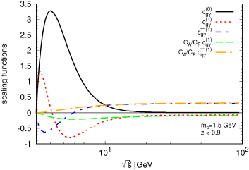
Figure 2: Scaling functions as function of $\sqrt{\hat{s}}$, where $C_{A}=3,~{}C_{F}=4/3$.

Already at this stage, one can note then that, at large $\hat{s}$, the NLO cross section will be proportional to $\ln({M_{\pazocal{Q}}^{2}}/{\mu_{F}^{2}})$ and a process-dependent coefficient, $\overline{c}^{(1)}_{\gamma i}(\hat{s}\to\infty,m_{Q}^{2})$, which only comes on the real-emission contributions, like for $\eta_{Q}$ hadroproduction [29].

Fig. 3 shows the $\sqrt{s_{\gamma p}}$-dependence of $\sigma_{\gamma p}$ for $J/\psi$ photoproduction integrated over $z<0.9$ and $P_{T}$, for different choices of $\mu_{R}$ and $\mu_{F}$ among $M_{J/\psi}\times(0.5,1,2)$, using the CT18NLO PDF set [54] and with a $20\%$ feed-down contribution from $\psi^{\prime}$ decay (like in [7]). We expect the $b$ feed down on the $P_{T}$-integrated yields to be on the order of 5% and we do not include it as it can be experimentally removed. For $\Upsilon(1S)$ photoproduction, we have estimated the feed-down contributions from $\Upsilon(2S)$ to be 12.5$\%$ and from $\Upsilon(3S)$ to be 2.2$\%$.

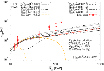
Figure 3: LO and NLO $\sigma_{\gamma p}$ as a function of $\sqrt{s_{\gamma p}}$ for $J/\psi$ photoproduction for different scale choices (with the notation $\xi_{R,F}\equiv\mu_{R,F}/M_{J/\psi}$) compared with experimental data: H1 [13], FTPS [56], NA14 [57].

The long dashed grey curve is the LO cross section for $\mu_{R}=M{Q}$ and $\mu_{F}=0.86~{}M{Q}$. We have checked that it remains positive for any $\mu_{R}$ and $\mu_{F}$ scale choice which is expected provided that the PDFs are positive. It happens to reasonably account for the available experimental values if one notes that the theoretical uncertainties from the scales, the mass and $R(0)$ (not shown) are significant. All other curves represent the NLO cross section for different scale choices. In two cases, the NLO cross section becomes negative as $s_{\gamma p}$ increases. Anticipating the results of the next section, the same behaviour is obtained with other well-known PDF sets (MSHT20 [58], NNPDF31 [59]). As for $\Upsilon(1S)$, the cross section remains positive in the considered energy range for any realistic scale choice, like for $\eta_{b}$ hadroproduction up to 100 TeV [29]. Let us now discuss the origin of such an unphysical behaviour for $J/\psi$ photoproduction and propose a solution to it.

2.5 A new scale prescription to cure the unphysical behaviour of the NLO quarkonium photoproduction cross section

From the above discussion, there can only be two sources of negative partonic cross sections: the loop amplitude via interference with the Born amplitude and the real emissions via the subtraction of the IR poles from the initial-emission collinear singularities. As we will argue now, the latter subtraction is the source of the negative cross section which we have just uncovered. As it was mentioned before, such divergences are removed by subtraction into the PDFs via AP-CT and the high-energy limit of the resulting partonic cross section takes the form:

$$\lim_{\hat{s}\rightarrow\infty}\hat{\sigma}_{\gamma i}^{\rm NLO}\propto\left({\log\frac{M_{\pazocal{Q}}^{2}}{\mu_{F}^{2}}+A_{\gamma i}}\right),A_{\gamma g}=A_{\gamma q},$$ (4)

where $A_{\gamma i}={c_{\gamma i}^{(1)}(\hat{s}\to\infty,m_{Q}^{2})}/{\overline{c}^{(1)}_{\gamma i}(\hat{s}\to\infty,m_{Q}^{2})}$ are the coefficients of the finite term of NLO cross section in the high-energy limit. As can be seen from Fig. 2, $A_{\gamma i}$ is negative for $z<0.9$, i.e. $-0.29$. It is also clear from Fig. 2 that $A_{\gamma g}=A_{\gamma q}$.

Unless $\mu_{F}$ is sufficiently smaller than $M_{\pazocal{Q}}$ in order to compensate $A_{\gamma i}$, $\lim\limits_{\hat{s}\rightarrow\infty}\hat{\sigma}_{\gamma i}^{\rm NLO}$ is negative, like for $\eta_{Q}$ [29] and it is another clear case of oversubtraction by the AP-CT. Indeed, in this limit, the virtual contributions are suppressed; only the real emissions contribute via their square. As such, they can only yield positive partonic cross sections before the subtraction of the initial-state collinear divergences. Since, after their subtraction, the partonic cross section is negative, it has to come from the AP-CT. This is what we refer to as oversubtraction by the AP-CT.

In principle, the negative term from the AP-CT should be compensated by the evolution of the PDFs according to the DGLAP equation. Yet, for the $\mu_{F}$ values on the order of the natural scale of these processes, the PDFs are not evolved much and can sometimes be so flat for some PDF parametrisations that the large $\hat{s}$ region still significantly contributes. This results in negative values of the hadronic cross section. Indeed, $A_{\gamma g}$ and $A_{\gamma q}$ are process-dependent, while the DGLAP equations are process-independent, which necessarily makes the compensation imperfect. Going to NNLO and even higher, this should naturally improve. If one has only NLO computations, this is however greatly problematic. A solution to this problem is [29] to force the partonic cross section to vanish in this limit, whose contribution should in principle be damped down by the PDFs.

According to this prescription, one needs to choose $\mu_{F}$ such that $\lim\limits_{\hat{s}\rightarrow\infty}\hat{\sigma}_{\gamma i}^{\rm NLO}=0$. It happens to be possible since $A_{\gamma g}=A_{\gamma q}$. This amounts to consider that all the QCD corrections are in the PDFs [29]. From Eq. (4), we have:

$$\mu_{F}=\hat{\mu}_{F}={M_{\pazocal{Q}}e^{A_{\gamma i}/2}=M_{\pazocal{Q}}{\rm exp}\left(\frac{c_{\gamma i}^{(1)}({\hat{s}\to\infty},m_{Q}^{2})}{2\overline{c}^{(1)}_{\gamma i}({\hat{s}\to\infty},m_{Q}^{2})}\right)}.$$ (5)

Using the scaling function of Fig. 2 when one fully integrates over $P_{T}$ and over $z<0.9$, one gets $\hat{\mu}_{F}={0.86}M_{\pazocal{Q}}$. From now on, all our NLO results will be shown with this value of the factorisation scale.

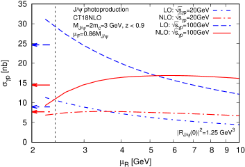
Figure 4: $\mu_{R}$ dependence of $\sigma_{\gamma p}$ at LO and NLO for 2 values of $\sqrt{s_{\gamma p}}$, where the arrows point at the values of $\sigma_{\gamma p}$ for $\mu_{R}=3$ GeV. The vertical dashed line delimitates the $\mu_{R}$ region which we use to compute the cross section (see text).

On Fig. 4, one can see the LO (in blue) and NLO (in red) $\mu_{R}$ dependence of $\sigma_{\gamma p}$ for $J/\psi$ photoproduction, still using CT18NLO and integrated over $P_{T}$ and over $z<0.9$, at two values of $\sqrt{s_{\gamma p}}=20$ GeV (short and long dash-dotted lines) and $\sqrt{s_{\gamma p}}=100$ GeV (solid and dashed lines). In both cases, the $\mu_{R}$ sensitivity is drastically reduced at NLO. However, one notes that at the higher energy, for $\mu_{R}\sim M_{J/\psi}$, $\sigma^{\rm NLO}_{\gamma p}$ is twice smaller than $\sigma^{\rm LO}_{\gamma p}$ (see the arrows by the $y$ axis). This is due to a large negative contribution from the loops (see the negative dip in the $c_{\gamma g}^{(1)}$ in Fig. 2). Since the LO and NLO cross section are however similar for $\mu_{R}\sim 2M_{J/\psi}$, the question of the natural scale of the process naturally arises. In fact, as the Born process is $\gamma g\to\pazocal{Q}g$, it appears reasonable to consider $\sqrt{\hat{s}}$ rather than $M{Q}$. A quick LO computation for the $J/\psi$ case shows that $\sqrt{\langle\hat{s}\rangle}$ ranges from 4 GeV at low hadronic energies up to even 10 GeV at high hadronic energies. In what follows, we thus consider $\mu_{R}$ within the range $[2.5:10]$ GeV for $J/\psi$ and, for $\Upsilon(1S)$, $\mu_{R}\in[8:32]$ GeV (with $\mu_{R}=5(16)$ GeV being the center of this range in the two cases) at both LO and NLO and for $\mu_{F}$ at LO. The procedure for $\mu_{F}$ at NLO is discussed in the next section.

2.6 Scale fixing and theoretical uncertainties

Just as we have discussed above, theoretical uncertainties of perturbative computations including radiative corrections arise from the appearances of unphysical scales, usually $\mu_{R}$ and $\mu_{F}$. In principle, predictions of physical observables, e.g. a cross section, should not depend on them. This would only be so if all radiative corrections could be accounted for. At NLO, it is far from being the case and the scale dependences can be strong, so strong that some results are sometimes unphysical like in the process under discussion for some (reasonable) $\mu_{F}$ values.

In general, the scale dependence is however mild (like for $\mu_{R}$ here) and evaluating observables at natural values of the scales, i.e. those entering the kinematics of the process, yield to good predictions, which usually improve at NNLO and so forth. Since the scale dependences are meant to disappear in all-order computations, one can revert the argument and consider that the scale dependences give us some information about the impact of higher orders. This is why one varies the scale, like we have discussed at the end of the previous section, hoping to seize up some theoretical uncertainties from Missing-Higher Orders (MHO) in the jargon. This is however not done without ambiguity, to say the least, as the resulting uncertainties fully depend on the range of scale variation, conventionally chosen to be a multiplicative factor 2 for historical but unclear reasons. Whatever the variation should be, one then faces an apparent impossibility with our scale-fixing prescription: how to vary a scale which is fixed?

To address this issue, it is necessary to go back to the very motivation of scale-fixing criteria. Like for our scale prescription, the other prescriptions (PMS [61], BLM-PMC [62, 63, 64], FAC [65, 66]) stem from physical pictures: the result should be stable, the results should be maximally conformal, the convergence should be as fast as possible or, like in our case, the result should exhibit no over-subtraction of collinear singularities inside the PDFs. The question is then how much one can depart from this expectation? Presumably, the scale value from a given prescription will not be the same at NLO and NNLO for instance. One could then try to derive the NLO scale from its formal expression artificially corrected by a typical NNLO corrections scaling like $\alpha_{s}/\pi$, on the order of unity in our case. This would provide a range of prescribed scales that we could plug in the NLO computation to get a scale uncertainty. In our case, instead of forcing $\log\frac{M_{\pazocal{Q}}^{2}}{\mu_{F}^{2}}+A_{\gamma i}$ to vanish, one could consider a range of $\mu_{F}$ such that its absolute value is bounded below unity. As such, we would probe the robustness of the scale-fixing criteria against expected higher-order corrections. This seems a very elegant solution for which the range of $\mu_{F}$ is $1/\sqrt{e}\leq\mu_{F}/\hat{\mu}_{F}\leq\sqrt{e}$.

There is however a caveat to compare it with the usual way, not because of the above solution, but because the conventional method of scale variation by 2 is purely arbitrary. For meaningful comparisons, the range of variation should be accounted for. After all, what one looks after is the scale dependence. A natural way to proceed should instead be to compute $d\sigma/d\ln\mu$ which would then be a local estimation of the scale dependence. Assuming that the variation by 2 is an approximate way to numerically evaluate this derivative, the connection between both requires to include a $\ln 2$ factor and $\ln 2/\ln{e}$ for the proposal above. We refer to B for more details.

In this context, we will show a NLO $\mu_{F}$ scale uncertainty derived from $\ln{2}\times d\sigma/d\ln\mu$, in fact very similar to that obtained from $1/\sqrt{e}\leq\mu_{F}/\hat{\mu}_{F}\leq\sqrt{e}$ rescaled by $\ln 2/\ln{e}$.

3 Results

Having discussed our methodology, let us now present and analyse our results for $J/\psi$ and $\Upsilon(1S)$ photoproduction cross sections computed at NLO with the $\hat{\mu}_{F}$ prescription.

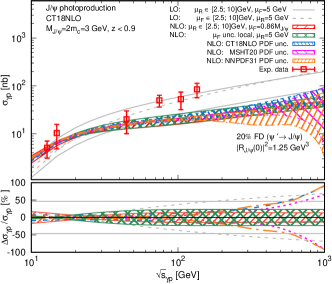
(a)

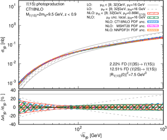
(b)

Figure 5: (Upper panels) $\sigma_{\gamma p}$ dependence on $\sqrt{s_{\gamma p}}$, (lower panels) $\Delta\sigma_{\gamma p}/\sigma_{\gamma p}$ dependence on $\sqrt{s_{\gamma p}}$ for (a) $J/\psi$ and (b) $\Upsilon(1S)$ inclusive photoproduction with the $\mu_{R}$ and the PDF uncertainties

On Fig. 5a and Fig. 5b, we have plotted (upper panel) the cross sections $\sigma_{\gamma p}$ and (lower panel) its (scale and PDF) relative uncertainty as functions of $\sqrt{s_{\gamma p}}$ for respectively $J/\psi$ and $\Upsilon(1S)$ photoproduction for different PDF sets: CT18NLO [54], MSHT20nlo_as118 [58], NNPDF31_nlo_as_0118_hessian [59]. Let us first discuss Fig. 5a. The LO cross section (2 solid and 2 dashed grey lines) relatively well describes the experimental data points in red with somewhat large uncertainties at large $\sqrt{s_{\gamma p}}$. The NLO cross section is systematically smaller and one notes that the NLO $\mu_{R}$ uncertainty (red hatched band) is reduced compared to the LO one, as expected from Fig. 4. The NLO $\mu_{F}$ uncertainty we obtained is well-behaved without any negative values anymore and is smaller than the LO one at large $\sqrt{s_{\gamma p}}$.

The PDF uncertainties at NLO from CT18NLO, MSHT20nlo_as118 and NNPDF31_nlo_as_0118_hessian are shown by respectively the blue, magenta and orange hatched bands. At large $\sqrt{s_{\gamma p}}$, which corresponds to the low-$x$ region in the proton, they naturally grow and eventually become larger than the $\mu_{R}$ uncertainty. Even though it is not an observable physical quantity, we note that with our present set-up (scheme and scale choice) the relative contribution from the $\gamma q$ fusion channel is relatively constant and close to 5% from 20 GeV and above, about 95% then comes from $\gamma g$ fusion. The three PDFs we have chosen are representative of what is available from fixed-order analyses. However, they are known [67] to be artificially suppressed at low $x$ and low scales and can even show a local mininum which then distorts in the energy dependence of $\eta_{c}$ hadroproduction cross section [29]. As such, the possibility remains, that even within their increasing uncertainties, such present PDF sets are possibly unsuited to reliably describe quarkonium production data. Using the latter to redetermine the former is then certainly something which should be attempted.

The increase of the PDF uncertainty is even more visible on the relative uncertainty plots Fig. 5a (lower panel) for $\mu_{R}=5$ GeV. Above 300 GeV, these are clearly larger than the $\mu_{R}$ one which slightly grows above 50 GeV due to the on-set of the negative contributions from the loop corrections (see below) and the $\mu_{F}$ one which also slightly grows above 20 GeV, where it happens to coincidentally vanish for a wide range of values. As for the $\Upsilon(1S)$ case, shown on Fig. 5b, the reduction of the $\mu_{R}$ uncertainty at NLO is further pronounced while the PDF and $\mu_{F}$ uncertainties remain similar.

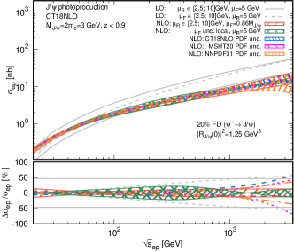
(a)

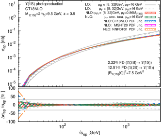
(b)

Figure 6: (Upper panels) $\sigma_{ep}$ as a function of $\sqrt{s_{ep}}$, (lower panels) $\Delta\sigma_{ep}/\sigma_{ep}$ as a function of $\sqrt{s_{ep}}$ for (a) $J/\psi$ and (b) $\Upsilon(1S)$ inclusive photoproduction with its $\mu_{R}$ and the PDF uncertainties.

In the $J/\psi$ case, it is clear that it will be important to have at our disposal computations at NNLO accuracy. As Krämer noted [27] long ago, the “virtual+soft” contributions, encapsulated in $c^{(1)}$, are significantly more negative than for open heavy-flavour production [69]. He suggested that this destructive interference with the Born order amplitude could be due to the momentum transfer of the exchanged virtual gluon, more likely to scatter the $Q\bar{Q}$ pair outside the static limit (${\bf p}\simeq 0$). At NNLO, these one-loop amplitudes will be squared, the two-loop amplitudes will interfere with the Born amplitudes and the amplitudes of the one-loop corrections to the real-emission graphs will also interfere with the real-emission amplitudes. Unless the latter two are subject to the same strong destructive interference effect, one might expect relatively large positive NNLO corrections bringing the cross section close to the upper limit of the LO range and then in better agreement with existing, yet old, data.

At NNLO, we also expect a further reduction of the $\mu_{R}$ and $\mu_{F}$ uncertainties. This is particularly relevant especially around $50-100$ GeV, which corresponds to the EIC region. This would likely allow us to better probe gluon PDFs using photoproduction data. Going further, differential measurements in the elasticity or the rapidity could provide a complementary leverage in $x$ to fit the gluon PDF, even in the presence of sub-leading $v$ colour-octet contributions. Indeed, these would likely exhibit a very similar dependence on $x$. As we will see now, the expected yields at future facilities, in particular for charmonia, are clearly large enough to perform such differential measurements.

Let us now look at electron-proton cross sections as functions of $\sqrt{s_{ep}}$ for $J/\psi$ (Fig. 6a) and $\Upsilon(1S)$ photoproduction (Fig. 6b). To obtain them, Eq. (3) was convoluted with the corresponding proton PDFs and a photon flux from the electron. We have used the same photon flux as in [7].

On Fig. 6a and Fig. 6b, the same colour code and the same parameters as for Fig. 5a and Fig. 5b have been used. For $\sigma_{ep}$, one can see the same trends for the $\mu_{R}$ and PDF uncertainties as for $\sigma_{\gamma p}$. It is only at the LHeC energies and above that one could expect to constrain better the PDF uncertainty with such total cross section measurements unless we have at our disposal NNLO computations with yet smaller scale uncertainties.

Exp.	$\sqrt{s_{ep}}$	${\cal L}$ (fb${}^{-1})$	$N_{J/\psi}$	$N_{\Upsilon(1S)}$
EicC	16.7	100	$1.5^{+0.3}_{-0.2}\cdot 10^{6}$	$2.3^{+1.1}_{-1.4}\cdot 10^{0}$
AMBER	17.3	1	$1.6^{+0.3}_{-0.3}\cdot 10^{4}$	$<1$
EIC	45	100	$8.5^{+0.5}_{-1.0}\cdot 10^{6}$	$6.1^{+0.7}_{-0.8}\cdot 10^{2}$
EIC	140	100	$2.5^{+0.1}_{-0.4}\cdot 10^{7}$	$7.6^{+0.3}_{-0.7}\cdot 10^{3}$
LheC	1183	100	$9.3^{+2.9}_{-2.9}\cdot 10^{7}$	$8.1^{+0.4}_{-0.7}\cdot 10^{4}$
FCC-eh	3464	100	$1.6^{+0.2}_{-1.0}\cdot 10^{8}$	$1.8^{+0.1}_{-0.2}\cdot 10^{5}$

Table 1: Expected number of detected quarkonia at NLO at different $\sqrt{s_{ep}}$ (in GeV) corresponding to future facilities (using CT18NLO, $\mu_{R}=5$ GeV for $J/\psi$ and $\mu_{R}=16$ GeV for $\Upsilon(1S)$, $\mu_{F}=\hat{\mu}_{F}$) for $\epsilon_{detect}=85\%$ via the decay channels to $\mu^{+}\mu^{-}$ and $e^{+}e^{-}$, namely $\epsilon^{J/\psi}_{\ell^{+}\ell^{-}}\approx 0.1$, and $\epsilon^{\Upsilon(1S)}_{\ell^{+}\ell^{-}}\approx 0.04$.

In Table 1, we provide estimations of the expected number of $J/\psi$ and $\Upsilon(1S)$ possibly detected at the different $ep$ c.m. energies of planned experiments. As it can be seen, the expected yields are always very large for $J/\psi$ which will clearly allow for a number of differential measurements in $z$, $y$ or $\sqrt{s_{\gamma p}}$. These could then be used to reduce the impact of partially correlated theoretical uncertainties, from the scales and the heavy-quark mass affecting these photoproduction cross sections, in order to bring about some additional constraints on the PDFs at low scales, in particular the gluon one. For $\Upsilon(1S)$, the yields should be sufficient to extract cross sections at the EIC, LHeC and FCC-eh even below their nominal luminosities.

One can also estimate the expected number of detected $\psi^{\prime},~{}\Upsilon(2S),~{}\Upsilon(3S)$ using the following relations $N_{\psi^{\prime}}\simeq 0.07\times N_{J/\psi}$,$N_{\Upsilon(2S)}\simeq 0.4\times N_{\Upsilon(1S)}$, $N_{\Upsilon(3S)}\simeq 0.3\times N_{\Upsilon(1S)},$ derived from the values of $|R_{\pazocal{Q}}(0)|^{2}$ and of the branching fractions to leptons. Using the above relations and the values in Table 1, one can see that the yield of $\psi^{\prime}$ should be measurable everywhere and the yields of $\Upsilon(2S)$ and $\Upsilon(3S)$ are close to about half of that of $\Upsilon(1S)$ and should be measurable at the EIC, LHeC and FCC-eh. The proximity between the $\Upsilon(nS)$ yields follows from their similar $|R_{\pazocal{Q}}(0)|^{2}$ and leptonic branchings.

4 A note on $P_{T}$-differential cross sections

As announced, the present study focuses on the fully $P_{T}$-integrated case. If, instead, one is interested in $P_{T}$-differential cross sections, our prescription for a single scale process would not work as it stands. Indeed, one has to be cautious that a class of real-emission NLO corrections (Fig. 1c) is kinematically enhanced by $(P_{T}/M{Q})^{2}$ with respect to the Born contributions. Considering the expected $P_{T}$ behaviour of the scaling functions entering the definition of $\hat{\mu}_{F}$, one finds that $c_{\gamma i}^{(1)}$ (which contains these contributions) is enhanced with respect to $\overline{c}^{(1)}_{\gamma i}$ (which only arises from the collinear contributions).

This would result in $\hat{\mu}_{F}(P_{T})$ scaling as $M{Q}\times\exp(P_{T}/M{Q})$. This can easily be explained if one reminds that our scale prescription effectively amounts to recast, at large partonic energies, all the NLO corrections in the PDF folded with the Born cross section. This would then be done, at large $P_{T}$, by trying to get those $P_{T}$-enhanced contributions entirely from the PDF evolution via an unphysically large $\mu_{F}$. At large $P_{T}$, the natural scale should instead be on the order of $P_{T}$ and not $M{Q}\times\exp(P_{T}/M{Q})$.

Common dynamical scale choices for $P_{T}$-differential cross sections are $(0.5,1,2)\times m_{T}$ with $m_{T}=\sqrt{M{Q}^{2}+P_{T}^{2}}$. Two possible choices scaling like $m_{T}$ at large $P_{T}$ and compatible with $\hat{\mu}_{F}$ when integrated over $P_{T}$ would be (i) $\alpha\times m_{T}$ with $\alpha$ fixed such that $\hat{\mu}_{F}=\alpha\sqrt{M{Q}^{2}+\langle P_{T}^{2}\rangle}$ and (ii) $\sqrt{(\beta\times M{Q})^{2}+P_{T}^{2}}$ with $\beta$ fixed such that $\hat{\mu}_{F}=\sqrt{(\beta M{Q})^{2}+\langle P_{T}^{2}\rangle}$. At HERA energies [13], $\langle P_{T}^{2}\rangle\simeq 2.5$ GeV² for $J/\psi$, this gives $\alpha=0.77$ and $\beta=0.7$. The former choice is shown on Fig. 7 (red boxes) and compared to cross section obtained with a fixed $\mu_{F}=\hat{\mu}_{F}$ for different $\mu_{R}$ (hashed red histogram). All choices give similar results which are compatible with the latest H1 data [18]. Predictions for the EIC at 140 GeV are also given. They confirm predictions given in our previous study [7] with an approximate NLO computation.

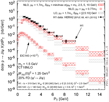
Figure 7: LO and NLO $d\sigma_{ep}/dP_{T}$ as a function of $P_{T}$ for $J/\psi$ photoproduction for different scale choices at HERA compared with the latest H1 experimental data [18] and at the EIC140.

5 Conclusions

Like for other charmonium production processes [71, 72, 29], we have observed the appearance at NLO of negative total cross section which we attribute to an oversubtraction of collinear divergences into the PDF via AP-CT in the $\overline{\text{MS}}$ scheme. We applied the $\hat{\mu}_{F}$ prescription proposed in [29], which up to NLO corresponds to a resummation of such collinear divergences in High-Energy Factorisation (HEF) [73]. Expressing this integrated cross section in terms of scaling functions exhibiting its explicit $\mu_{R}$ and $\mu_{F}$ scale dependencies, we have found that, for $z<0.9$, the optimal factorisation scale is $\hat{\mu}_{F}={0.86}M{Q}$ which falls well within the usual ranges of used values. Like for $\eta_{c}$ hadroproduction, such a factorisation-scale prescription indeed allows one to avoid negative NLO cross sections, but it apparently prevents one from studying the corresponding factorisation-scale uncertainties. We have thus elaborated on two approaches to study such scale uncertainties when one scale is fixed by a physical argument. We were not aware of such ideas before and these clearly deserve dedicated studies in the future.

We have seen that the NLO $\mu_{R}$ uncertainties get reduced compared to the LO ones but slightly increase around 50 GeV, because of rather large (negative) interferences between the one-loop and Born amplitudes. As mentioned before, these ”virtual+soft” contributions are significantly more negative than for open heavy-flavour production. While Krämer suggested that the difference could stem from the static limit ($\mathbf{p}\simeq 0$) specific to the non-relativistic quarkonia, from which one easily departs when gluon exchanges occur, it will certainly be very instructive to have NNLO computations to see whether such one-loop amplitudes squared would bring the cross section back up close to the LO one or whether the interference between the two-loop and the Born amplitudes and between the real-virtual and the real amplitudes would be also negative and large.

Our evaluated $\mu_{F}$ uncertainties at NLO are also reduced compared to those at LO at large $\sqrt{s_{\gamma p}}$ which were totally out of control before the application of the $\hat{\mu}_{F}$ prescription. We see that as a very encouraging sign.

In any case, at NNLO, it is reasonable to expect a further reduction of the scale uncertainties compared to the NLO results. We have also briefly addressed the application of our scale prescription to $P_{T}$-differentical cross sections and proposed choices scaling like $m_{T}$ at large $P_{T}$ while compatible with $\hat{\mu}_{F}={0.86}M{Q}$ when $P_{T}$ is integrated over.

We have also qualitatively investigated the possibility to constrain PDFs using future $J/\psi$ and $\Upsilon(1S)$ photoproduction data. Indeed, present PDF sets are possibly [29] unsuited to reliably describe high-energy quarkonium production data. Restricting to conventional sets, we have seen that PDF uncertainties get larger than the (NLO) $\mu_{R}$ and $\mu_{F}$ uncertainties with the growth of the $\gamma p$ c.m. energy, in practice from around $300$ GeV, i.e. for $x$ below $0.01$. Although this is above the reach of the future EIC, we hope that with NNLO predictions at our disposal in the future, with yet smaller $\mu_{R}$ and $\mu_{F}$ uncertainties, one could set novel constraints on PDFs with such EIC measurements. Given our estimated counting rates for 100 fb^-1 of $ep$ collisions, we expect that a number of differential measurements will be possible to reduce the impact of highly or even partially correlated theoretical uncertainties, including the contamination of higher-$v$ corrections such as the colour-octet contributions. These, along with the forthcoming HL-LHC measurements [21], should also definitely help to improve our understanding of the quarkonium-production mechanisms.

Strictly speaking our predictions for $J/\psi$ and $\psi^{\prime}$ only regard the prompt yields. An evaluation at NLO of the beauty production cross section points at a feed-down fraction at the 5% level. Given the larger size of the other uncertainties and the possibility to remove it experimentally, we have neglected it. In general though, it will be useful to have a dedicated experimental measurements at the EIC at least to measure the beauty feed down. It may become more significant at low $z$ where the resolved-photon contribution could set in at high $\sqrt{s_{ep}}$, like we have seen [7] it to become the dominant source of $J/\psi$ at large $P_{T}$.

Acknowledgements

We thank S.J. Brodsky, Y. Dokshitzer, M. Mangano, M. Nefedov and H. Sazdjian for useful discussions, L. Manna for a NLO estimate of the $b$ photoproduction cross section and K. Lynch for comments on the manuscript. This project has received funding from the European Union’s Horizon 2020 research and innovation programme under grant agreement No. 824093 in order to contribute to the EU Virtual Access NLOAccess. This project has also received funding from the Agence Nationale de la Recherche (ANR) via the grant ANR-20-CE31-0015 (“PrecisOnium”) and via the IDEX Paris-Saclay ”Investissements d’Avenir” (ANR-11-IDEX-0003-01) through the GLUODYNAMICS project funded by the ”P2IO LabEx (ANR-10-LABX-0038)” and through the Joint PhD Programme of Université Paris-Saclay (ADI). This work was also partly supported by the French CNRS via the IN2P3 project GLUE@NLO, via the Franco-Chinese LIA FCPPL (Quarkonium4AFTER) and via the Franco-Polish EIA (GlueGraph). M.A.O.’s work was partly supported by the ERC grant 637019 “MathAm”. C.F. has been also partially supported by Fondazione di Sardegna under the project “Proton tomography at the LHC”, project number F72F20000220007 (University of Cagliari), and is thankful to the Physics Department of Cagliari University for the hospitality and support for his visit, during which part of the project was done.

Appendix A Leptonic width and wave function at the origin

Up to NNLO, one has [48, 49] (for $\mu_{\rm NRQCD}=m_{Q}$):

$$\Gamma_{\ell\ell} =\frac{4\pi\alpha^{2}e_{Q}^{2}f_{\pazocal{Q}}^{2}}{3M_{\pazocal{Q}}},f_{\pazocal{Q}}=\sqrt{\frac{3}{\pi M_{\pazocal{Q}}}|R(0)|^{2}}\Bigg{[}1-\frac{8}{3}\frac{\alpha_{s}(\mu_{R})}{\pi}$$ (6)

$$-\Biggl{(}44.55-0.41n_{lf}-\frac{2}{3}\beta_{0}\ln{\frac{M_{\pazocal{Q}}^{2}}{4\mu_{R}^{2}}}\Biggr{)}\Biggl{(}\frac{\alpha_{s}(\mu_{R})}{\pi}\Biggr{)}^{2}\Bigg{]},$$

where $n_{lf}$ is the number of active light flavours, $\alpha$ is the electromagnetic coupling constant, $\alpha_{s}$ is the strong interaction coupling, $M_{\pazocal{Q}}$ is the $\pazocal{Q}$ mass, $e_{Q}$ is the magnitude of the heavy-quark charge (in units of the electron charge). In Table 2, we have gathered the resulting radial part of the Schrödinger wave function at the origin of the configuration space at LO, NLO and NNLO for $J/\psi$ and $\Upsilon(1S)$, which were computed from Eq. (6) with the measured value of $\Gamma_{\ell\ell}$ [55].

$\alpha_{s}$	$|R_{J/\psi}(0)|^{2}_{\rm LO}$	$|R_{J/\psi}(0)|^{2}_{\rm NLO}$	$|R_{J/\psi}(0)|^{2}_{\rm NNLO}$
[0.18,0.34]	0.52	[0.73,1.04]	[1.32,12.61]
$\alpha_{s}$	$|R_{\Upsilon(1S)}(0)|^{2}_{\rm LO}$	$|R_{\Upsilon(1S)}(0)|^{2}_{\rm NLO}$	$|R_{\Upsilon(1S)}(0)|^{2}_{\rm NNLO}$
[0.14,0.18]	4.90	[6.31,6.83]	[8.63,10.38]

Table 2: Values of $|R(0)|^{2}$ in GeV³ extracted from the corresponding leptonic widths [55] at LO, NLO and NNLO.

Appendix B Estimating the ‘scale’ uncertainty for a fixed scale

Scale uncertainties are historically evaluated in pQCD by a multiplicative variation by a factor of 2. Assuming that the corresponding $\mu$ uncertainty, defined as $\sigma\pm\Delta\sigma$, is evaluated via

$$\Delta\sigma(\mu)=\frac{\left|\sigma(2\mu)-\sigma(\mu/2)\right|}{2}\,,$$ (7)

it is easy to note that wider variations necessarily lead to larger uncertainties and narrower ones to smaller uncertainties. However, as pointed out above, the common practice is to use such a factor 2 which then lead to the usual 7- or 9-point variation technique to estimate the envelope corresponding to the factorisation and renormalisation scale uncertainty.

To ‘fix’ this ambiguity and yet allowing one to make the variation as wide or narrow as we wish, we propose to rescale it as follows

$$\Delta_{\xi}\sigma(\mu)=\left|\frac{\sigma(\xi\mu)-\sigma(\mu/\xi)}{2}\frac{\ln 2}{\ln\xi}\right|.$$ (8)

For $\xi=2$, one recovers the usual uncertainty.

With this definition, one can consider $\Delta_{\xi}\sigma$ evaluated locally (i.e. for a scale variation very close to $\mu$, thus for $\xi\to 1$). Such local evaluation is in fact simply connected to $\frac{\partial\sigma}{\partial\ln\mu}$ as

$$\lim_{\xi\to 1}\Delta_{\xi}\sigma=\ln{2}\times\left|\frac{\partial\sigma(\mu)}{\partial\ln\mu}\right|\,.$$ (9)

References

- [1] J.-P. Lansberg, “New Observables in Inclusive Production of Quarkonia,” Phys. Rept. 889 (2020) 1–106, arXiv:1903.09185 [hep-ph].
- [2] A. Andronic et al., “Heavy-flavour and quarkonium production in the LHC era: from proton–proton to heavy-ion collisions,” Eur. Phys. J. C76 no. 3, (2016) 107, arXiv:1506.03981 [nucl-ex].
- [3] N. Brambilla et al., “Heavy Quarkonium: Progress, Puzzles, and Opportunities,” Eur. Phys. J. C71 (2011) 1534, arXiv:1010.5827 [hep-ph].
- [4] J. P. Lansberg, “, and production at hadron colliders: A Review,” Int. J. Mod. Phys. A21 (2006) 3857–3916, arXiv:hep-ph/0602091 [hep-ph].
- [5] Quarkonium Working Group Collaboration, N. Brambilla et al., “Heavy quarkonium physics,” arXiv:hep-ph/0412158 [hep-ph].
- [6] M. Kraemer, “Quarkonium production at high-energy colliders,” Prog. Part. Nucl. Phys. 47 (2001) 141–201, arXiv:hep-ph/0106120 [hep-ph].
- [7] C. Flore, J.-P. Lansberg, H.-S. Shao, and Y. Yedelkina, “Large- inclusive photoproduction of in electron-proton collisions at HERA and the EIC,” Phys. Lett. B 811 (2020) 135926, arXiv:2009.08264 [hep-ph].
- [8] C. Flore, J.-P. Lansberg, H.-S. Shao, and Y. Yedelkina, “NLO inclusive photoproduction at large at HERA and the EIC,” SciPost Phys. Proc. 8 (2022) 011, arXiv:2107.13434 [hep-ph].
- [9] C.-H. Chang, “Hadronic Production of Associated With a Gluon,” Nucl. Phys. B172 (1980) 425–434.
- [10] E. L. Berger and D. L. Jones, “Inelastic Photoproduction of J/psi and Upsilon by Gluons,” Phys. Rev. D23 (1981) 1521–1530.
- [11] R. Baier and R. Ruckl, “Hadronic Collisions: A Quarkonium Factory,” Z. Phys. C19 (1983) 251.
- [12] G. T. Bodwin, E. Braaten, and G. P. Lepage, “Rigorous QCD analysis of inclusive annihilation and production of heavy quarkonium,” Phys. Rev. D51 (1995) 1125–1171, arXiv:hep-ph/9407339 [hep-ph]. [Erratum: Phys. Rev.D55,5853(1997)].
- [13] H1 Collaboration, S. Aid et al., “Elastic and inelastic photoproduction of mesons at HERA,” Nucl. Phys. B 472 (1996) 3–31, arXiv:hep-ex/9603005.
- [14] ZEUS Collaboration, J. Breitweg et al., “Measurement of inelastic photoproduction at HERA,” Z. Phys. C 76 (1997) 599–612, arXiv:hep-ex/9708010.
- [15] ZEUS Collaboration, S. Chekanov et al., “Measurements of inelastic and photoproduction at HERA,” Eur. Phys. J. C 27 (2003) 173–188, arXiv:hep-ex/0211011.
- [16] H1 Collaboration, C. Adloff et al., “Inelastic photoproduction of mesons at HERA,” Eur. Phys. J. C25 (2002) 25–39, arXiv:hep-ex/0205064 [hep-ex].
- [17] ZEUS Collaboration, S. Chekanov et al., “Measurement of J/psi helicity distributions in inelastic photoproduction at HERA,” JHEP 12 (2009) 007, arXiv:0906.1424 [hep-ex].
- [18] H1 Collaboration, F. Aaron et al., “Inelastic Production of Mesons in Photoproduction and Deep Inelastic Scattering at HERA,” Eur. Phys. J. C 68 (2010) 401–420, arXiv:1002.0234 [hep-ex].
- [19] ZEUS Collaboration, H. Abramowicz et al., “Measurement of inelastic and photoproduction at HERA,” JHEP 02 (2013) 071, arXiv:1211.6946 [hep-ex].
- [20] H. Jung, G. A. Schuler, and J. Terron, “J / psi production mechanisms and determination of the gluon density at HERA,” Int. J. Mod. Phys. A7 (1992) 7955–7988.
- [21] E. Chapon et al., “Prospects for quarkonium studies at the high-luminosity LHC,” Prog. Part. Nucl. Phys. 122 (2022) 103906, arXiv:2012.14161 [hep-ph].
- [22] D. Boer, U. D’Alesio, F. Murgia, C. Pisano, and P. Taels, “ meson production in SIDIS: matching high and low transverse momentum,” JHEP 09 (2020) 040, arXiv:2004.06740 [hep-ph].
- [23] R. Kishore, A. Mukherjee, and S. Rajesh, “Sivers asymmetry in the photoproduction of a and a jet at the EIC,” Phys. Rev. D101 no. 5, (2020) 054003, arXiv:1908.03698 [hep-ph].
- [24] U. D’Alesio, F. Murgia, C. Pisano, and P. Taels, “Azimuthal asymmetries in semi-inclusive production at an EIC,” Phys. Rev. D100 no. 9, (2019) 094016, arXiv:1908.00446 [hep-ph].
- [25] A. Bacchetta, D. Boer, C. Pisano, and P. Taels, “Gluon TMDs and NRQCD matrix elements in production at an EIC,” Eur. Phys. J. C80 no. 1, (2020) 72, arXiv:1809.02056 [hep-ph].
- [26] M. Kramer, J. Zunft, J. Steegborn, and P. M. Zerwas, “Inelastic J / psi photoproduction,” Phys. Lett. B 348 (1995) 657–664, arXiv:hep-ph/9411372.
- [27] M. Kraemer, “QCD corrections to inelastic J / psi photoproduction,” Nucl. Phys. B459 (1996) 3–50, arXiv:hep-ph/9508409 [hep-ph].
- [28] H1 Collaboration, S. Aid et al., “Elastic and inelastic photoproduction of mesons at HERA,” Nucl. Phys. B 472 (1996) 3–31, arXiv:hep-ex/9603005.
- [29] J.-P. Lansberg and M. A. Ozcelik, “Curing the unphysical behaviour of NLO quarkonium production at the LHC and its relevance to constrain the gluon PDF at low scales,” Eur. Phys. J. C 81 no. 6, (2021) 497, arXiv:2012.00702 [hep-ph].
- [30] A. Accardi et al., “Electron Ion Collider: The Next QCD Frontier: Understanding the glue that binds us all,” Eur. Phys. J. A 52 no. 9, (2016) 268, arXiv:1212.1701 [nucl-ex].
- [31] LHeC Study Group Collaboration, J. L. Abelleira Fernandez et al., “A Large Hadron Electron Collider at CERN: Report on the Physics and Design Concepts for Machine and Detector,” J. Phys. G 39 (2012) 075001, arXiv:1206.2913 [physics.acc-ph].
- [32] FCC Collaboration, A. Abada et al., “FCC Physics Opportunities: Future Circular Collider Conceptual Design Report Volume 1,” Eur. Phys. J. C 79 no. 6, (2019) 474.
- [33] B. Adams et al., “Letter of Intent: A New QCD facility at the M2 beam line of the CERN SPS (COMPASS++/AMBER),” arXiv:1808.00848 [hep-ex].
- [34] D. P. Anderle et al., “Electron-ion collider in China,” Front. Phys. (Beijing) 16 no. 6, (2021) 64701, arXiv:2102.09222 [nucl-ex].
- [35] P. Artoisenet, J. M. Campbell, J.-P. Lansberg, F. Maltoni, and F. Tramontano, “ Production at Fermilab Tevatron and LHC Energies,” Phys. Rev. Lett. 101 (2008) 152001, arXiv:0806.3282 [hep-ph].
- [36] J.-P. Lansberg, “On the mechanisms of heavy-quarkonium hadroproduction,” Eur. Phys. J. C 61 (2009) 693–703, arXiv:0811.4005 [hep-ph].
- [37] J.-P. Lansberg, “Real next-to-next-to-leading-order QCD corrections to and Upsilon hadroproduction in association with a photon,” Phys. Lett. B 679 (2009) 340–346, arXiv:0901.4777 [hep-ph].
- [38] B. Gong, J.-P. Lansberg, C. Lorce, and J. Wang, “Next-to-leading-order QCD corrections to the yields and polarisations of J/Psi and Upsilon directly produced in association with a Z boson at the LHC,” JHEP 03 (2013) 115, arXiv:1210.2430 [hep-ph].
- [39] J.-P. Lansberg and H.-S. Shao, “Production of versus at the LHC: Importance of Real Corrections,” Phys. Rev. Lett. 111 (2013) 122001, arXiv:1308.0474 [hep-ph].
- [40] J.-P. Lansberg and H.-S. Shao, “J/psi -pair production at large momenta: Indications for double parton scatterings and large contributions,” Phys. Lett. B751 (2015) 479–486, arXiv:1410.8822 [hep-ph].
- [41] J.-P. Lansberg, H.-S. Shao, and H.-F. Zhang, “ Hadroproduction at Next-to-Leading Order and its Relevance to Production,” Phys. Lett. B 786 (2018) 342–346, arXiv:1711.00265 [hep-ph].
- [42] H.-S. Shao, “Boosting perturbative QCD stability in quarkonium production,” JHEP 01 (2019) 112, arXiv:1809.02369 [hep-ph].
- [43] H. Fritzsch, “Producing Heavy Quark Flavors in Hadronic Collisions: A Test of Quantum Chromodynamics,” Phys. Lett. B 67 (1977) 217–221.
- [44] F. Halzen, “Cvc for Gluons and Hadroproduction of Quark Flavors,” Phys. Lett. B 69 (1977) 105–108.
- [45] H.-S. Shao, “HELAC-Onia: An automatic matrix element generator for heavy quarkonium physics,” Comput. Phys. Commun. 184 (2013) 2562–2570, arXiv:1212.5293 [hep-ph].
- [46] H.-S. Shao, “HELAC-Onia 2.0: an upgraded matrix-element and event generator for heavy quarkonium physics,” Comput. Phys. Commun. 198 (2016) 238–259, arXiv:1507.03435 [hep-ph].
- [47] R. Barbieri, R. Gatto, R. Kogerler, and Z. Kunszt, “Meson hyperfine splittings and leptonic decays,” Phys. Lett. B 57 (1975) 455–459.
- [48] A. Czarnecki and K. Melnikov, “Two loop QCD corrections to the heavy quark pair production cross-section in e+ e- annihilation near the threshold,” Phys. Rev. Lett. 80 (1998) 2531–2534, arXiv:hep-ph/9712222.
- [49] M. Beneke, A. Signer, and V. A. Smirnov, “Two loop correction to the leptonic decay of quarkonium,” Phys. Rev. Lett. 80 (1998) 2535–2538, arXiv:hep-ph/9712302.
- [50] P. Marquard, J. H. Piclum, D. Seidel, and M. Steinhauser, “Three-loop matching of the vector current,” Phys. Rev. D 89 no. 3, (2014) 034027, arXiv:1401.3004 [hep-ph].
- [51] CTEQ Collaboration, R. Brock et al., “Handbook of perturbative QCD: Version 1.0,” Rev. Mod. Phys. 67 (1995) 157–248.
- [52] J.-X. Wang, “Progress in FDC project,” Nucl. Instrum. Meth. A 534 (2004) 241–245, arXiv:hep-ph/0407058.
- [53] M. Butenschoen and B. A. Kniehl, “Complete next-to-leading-order corrections to J/psi photoproduction in nonrelativistic quantum chromodynamics,” Phys. Rev. Lett. 104 (2010) 072001, arXiv:0909.2798 [hep-ph].
- [54] T.-J. Hou et al., “New CTEQ global analysis of quantum chromodynamics with high-precision data from the LHC,” Phys. Rev. D 103 no. 1, (2021) 014013, arXiv:1912.10053 [hep-ph].
- [55] Particle Data Group Collaboration, P. A. Zyla et al., “Review of Particle Physics,” PTEP 2020 no. 8, (2020) 083C01.
- [56] B. H. Denby et al., “Inelastic and Elastic Photoproduction of J/ (3097),” Phys. Rev. Lett. 52 (1984) 795–798.
- [57] NA14 Collaboration, R. Barate et al., “Measurement of and Real Photoproduction on 6Li at a Mean Energy of 90-GeV,” Z. Phys. C 33 (1987) 505.
- [58] S. Bailey, T. Cridge, L. A. Harland-Lang, A. D. Martin, and R. S. Thorne, “Parton distributions from LHC, HERA, Tevatron and fixed target data: MSHT20 PDFs,” Eur. Phys. J. C 81 no. 4, (2021) 341, arXiv:2012.04684 [hep-ph].
- [59] NNPDF Collaboration, R. D. Ball et al., “Parton distributions from high-precision collider data,” Eur. Phys. J. C 77 no. 10, (2017) 663, arXiv:1706.00428 [hep-ph].
- [60] G. Altarelli, M. Diemoz, G. Martinelli, and P. Nason, “Total Cross-Sections for Heavy Flavor Production in Hadronic Collisions and QCD,” Nucl. Phys. B 308 (1988) 724–752.
- [61] P. M. Stevenson, “Optimized Perturbation Theory,” Phys. Rev. D 23 (1981) 2916.
- [62] S. J. Brodsky, G. P. Lepage, and P. B. Mackenzie, “On the Elimination of Scale Ambiguities in Perturbative Quantum Chromodynamics,” Phys. Rev. D 28 (1983) 228.
- [63] M. Mojaza, S. J. Brodsky, and X.-G. Wu, “Systematic All-Orders Method to Eliminate Renormalization-Scale and Scheme Ambiguities in Perturbative QCD,” Phys. Rev. Lett. 110 (2013) 192001, arXiv:1212.0049 [hep-ph].
- [64] X.-G. Wu, S. J. Brodsky, and M. Mojaza, “The Renormalization Scale-Setting Problem in QCD,” Prog. Part. Nucl. Phys. 72 (2013) 44–98, arXiv:1302.0599 [hep-ph].
- [65] G. Grunberg, “Renormalization Group Improved Perturbative QCD,” Phys. Lett. B 95 (1980) 70. [Erratum: Phys.Lett.B 110, 501 (1982)].
- [66] G. Grunberg, “Renormalization Scheme Independent QCD and QED: The Method of Effective Charges,” Phys. Rev. D 29 (1984) 2315–2338.
- [67] xFitter Developers’ Team Collaboration, H. Abdolmaleki et al., “Impact of low- resummation on QCD analysis of HERA data,” Eur. Phys. J. C 78 no. 8, (2018) 621, arXiv:1802.00064 [hep-ph].
- [68] A. Buckley, J. Ferrando, S. Lloyd, K. Nordström, B. Page, M. Rüfenacht, M. Schönherr, and G. Watt, “LHAPDF6: parton density access in the LHC precision era,” Eur. Phys. J. C 75 (2015) 132, arXiv:1412.7420 [hep-ph].
- [69] J. Smith and W. L. van Neerven, “QCD corrections to heavy flavor photoproduction and electroproduction,” Nucl. Phys. B 374 (1992) 36–82.
- [70] M. A. Ozcelik, “Constraining gluon PDFs with quarkonium production,” PoS DIS2019 (2019) 159, arXiv:1907.01400 [hep-ph].
- [71] M. L. Mangano and A. Petrelli, “NLO quarkonium production in hadronic collisions,” Int. J. Mod. Phys. A 12 (1997) 3887–3897, arXiv:hep-ph/9610364.
- [72] Y. Feng, J.-P. Lansberg, and J.-X. Wang, “Energy dependence of direct-quarkonium production in collisions from fixed-target to LHC energies: complete one-loop analysis,” Eur. Phys. J. C 75 no. 7, (2015) 313, arXiv:1504.00317 [hep-ph].
- [73] J.-P. Lansberg, M. Nefedov, and M. A. Ozcelik, “Matching next-to-leading-order and high-energy-resummed calculations of heavy-quarkonium-hadroproduction cross sections,” JHEP 05 (2022) 083, arXiv:2112.06789 [hep-ph].