Why diffusion-based preconditioning of Richards equation works: spectral analysis and computational experiments at very large scale.

Abstract

[Summary] We consider here a cell-centered finite difference approximation of the Richards equation in three dimensions, averaging for interface values the hydraulic conductivity $K=K(p)$, a highly nonlinear function, by arithmetic, upstream and harmonic means. The nonlinearities in the equation can lead to changes in soil conductivity over several orders of magnitude and discretizations with respect to space variables often produce stiff systems of differential equations. A fully implicit time discretization is provided by backward Euler one-step formula; the resulting nonlinear algebraic system is solved by an inexact Newton Armijo-Goldstein algorithm, requiring the solution of a sequence of linear systems involving Jacobian matrices. We prove some new results concerning the distribution of the Jacobians eigenvalues and the explicit expression of their entries. Moreover, we explore some connections between the saturation of the soil and the ill conditioning of the Jacobians. The information on eigenvalues justifies the effectiveness of some preconditioner approaches which are widely used in the solution of Richards equation. We also propose a new software framework to experiment with scalable and robust preconditioners suitable for efficient parallel simulations at very large scales. Performance results on a literature test case show that our framework is very promising in the advance towards realistic simulations at extreme scale.

, , , and (2022), Why diffusion-based preconditioning of Richards equation works: spectral analysis and computational experiments at very large scale., ArXiv, https://arxiv.org/abs/2112.05051.

1 Introduction

Groundwater flow in the unsaturated zone is a highly nonlinear phenomenon that can be modeled by the Richards equation, and there is a significant amount of research concerning different formulations and algorithms for calculating the flow of water through unsaturated porous media ^{1, 2, 3, 4, 5}.

The Richards equation is a time-dependent Partial Differential Equation (PDE) whose discretization leads to large nonlinear systems of algebraic equations, which often include coefficients showing large variations over different orders of magnitude. Typically, the variation in the coefficients is due to the use of a geostatistical model for hydraulic conductivity, allowing changes of many orders of magnitude from one cell to the next (heterogeneity) as well as correlations of values in each direction (statistical anisotropy). High heterogeneity and anisotropy in the problem and the presence of strong nonlinearities in the equation’s coefficients make the problem difficult to be solved numerically.

The main contribution of the present work is twofold. First, we investigate the spectral properties of the sequence of Jacobian matrices arising in the solution of the non linear systems of algebraic equations by a quasi-Newton method; these properties allow us to formulate a new theoretical justification for some preconditioning choices in solving Richards equation which are indeed current usual practices in the literature; to the best of our knowledge, this is the first theoretical formulation to support such common practices. Then, on the basis of the theoretical indications, we discuss a scalable and efficient parallel solution of a modified inexact quasi-Newton method with Krylov solvers and Armijo-Goldstein’s line search, i.e. Newton-like algorithms where the Newton correction linear equations are solved by a Krylov subspace method. To this aim, we interface the KINSOL package available from the Sundials project ⁶ with the most recent version of libraries for solving sparse linear systems by parallel Krylov solvers coupled with purely algebraic preconditioners ⁷, currently being extended in some EU-funded projects.

The work is organized as follows. First, in Section 2 we discuss the discretization of the Richards equation by means of cell-centered finite differences. Then, in Section 3, we summarize the inexact quasi-Newton method as implemented in the KINSOL framework. In Section 4 we propose an analysis of some spectral properties of the sequence of Jacobian matrices produced by the underlying Newton method. In Section 5, we describe some of the main features of the PSCToolkit parallel software framework, which we use to implement the computational procedure described in this paper.

The information produced by the spectral analysis of the Jacobian matrices is used in Section 5.2 to devise a preconditioning strategy for the Krylov subspace method and to present the preconditioners used in this study. Some numerical examples highlighting the computational performance of the proposed methods are then presented in Section 6. Finally, in Section 7 we draw our conclusion and briefly discuss future extensions.

2 Formulating the discrete problem

Flow in the vadose zone, which is also known as the unsaturated zone, has rather delicate aspects such as the parameters that control the flow, which depend on the saturation of the media, leading to the nonlinear problem described by the Richards equation. The flow can be expressed as a combination of Darcy’s law and the principle of mass conservation by

$$\frac{\partial\left(\rho\,\phi s(p)\right)}{\partial t}+\nabla\cdot q=0,$$

in which $s(p)$ is the saturation at pressure head $p$ of a fluid with density $\rho$ in terrain with porosity $\phi$, and $q$ is the volumetric water flux. By using Darcy’s law as

$$q=-K(p)\left(\nabla p+c\hat{z}\right),$$

for $K(p)$ the hydraulic conductivity, and $c$ the cosine of the angle between the downward $z$ axis $\hat{z}$ and the direction of the gravity force, we obtain that the overall equation has a diffusion as well as an advection term, the latter being related to gravity. For the sake of simplicity, we consider cases in which $c=1$, i.e. the advection acts only in the $z$ direction. There are two different forms of the Richards equation that differ in how they deal with the nonlinearity in the time derivative. The most popular form, which is the one considered here for a fluid that will always be water, permits to express the general equation as

$$\rho\,\phi\frac{\partial s(p)}{\partial t}-\nabla\cdot K(p)\nabla p-\frac{\partial K(p)}{\partial z}=f,$$ (1)

where $p(t)$ is the pressure head at time $t$, $s(p)$ is water saturation at pressure head $p$, $\rho$ is water density, $\phi$ is the porosity of the medium, $K(p)$ the hydraulic conductivity, $f$ represents any water source terms and $z$ is elevation. The equation is then completed by adding boundary and initial conditions. This formulation of the Richards equation is called the mixed form ^{1, 3} because the equation is parameterized in $p$ (pressure head) but the time derivative is in terms of $s$ (water saturation). Another formulation of the Richards equation is known as the head-based form, and is popular because the time derivative is written explicitly in terms of the pressure head $p$ ^{2, 3}.

It is important to note that in unsaturated flow both water content, $\phi s(p)$, and hydraulic conductivity, $K(p)$, are functions of the pressure head $p$. There are several empirical relations used to relate these parameters, including, e.g., the Brooks-Corey ⁸ model and the Van Genuchten model ². The Van Genuchten model is slightly more popular because it containts no discontinuities in the functions, unlike the Brooks-Corey model, and therefore avoids the risk of losing the uniqueness of the solution of the semidiscretized equation in space by the well-known Peano Theorem. A version of the Van Genuchten-Richards equation in mixed form model by Celia et al. ³ reported the following choices:

$$s(p)=\frac{\alpha(s_{s}-s_{r})}{\alpha+|p|^{\beta}}+s_{r},$$ (2)

and

$$K(p)=K_{s}\frac{a}{a+|p|^{\gamma}}$$ (3)

where the $\alpha,\beta,\gamma$, and $a$ are fitting parameters that are often assumed to be constant in the media; $s_{r}$ and $s_{s}$ are the residual and saturated moisture contents, and $K_{s}$ is the saturated hydraulic conductivity.

Small changes in the pressure head can change the hydraulic conductivity by several orders of magnitude, and $K(p)$ is a highly nonlinear function. The water content curve is also highly nonlinear as saturation can change drastically over a small range of pressure head values. It should be noted that these functions are only valid when the pressure head is negative; that is, the media is semi-saturated; when the media is fully saturated, $K=K_{s}$, $s(p)$ is equal to the porosity, and the Richards equation reduces to the Darcy linear equation; see the example in Figure 1.

Figure 1: Hydraulic conductivity $K(p)$ and volumetric water content $S(p)$ for parameters $\alpha=\texttt{1.611e+6}$, $\beta=3.96$ , $\gamma=4.74$, $a=\texttt{1.175e+6}$, $S_{s}=0.287$, $S_{r}=0.075$, $K_{s}=0.00944$ $\mathrm{c}\mathrm{m}\mathrm{/}\mathrm{s}$.

Typical uses of the Richards equation are to simulate infiltration experiments in the laboratory and in the field. These begin with initially dry soil, then water is added to the top of the core sample (or ground surface). These experiments require the simulation of fast changes in pressure head and saturation over the most nonlinear part of the Van Genuchten curves.

2.1 Cell-centered finite difference discretization

At the beginning of an infiltration experiment, the pressure head $p$ can be close to discontinuous. These large changes are also reflected in the nonlinear terms $K$ and $s(p)$. Taking into account the effect of the initial conditions, the time step can be severely limited if an inappropriate time discretization is chosen. Hydrogeologists are often interested in following the process until a steady state is achieved, which may take a long time; therefore, large time steps should be used to avoid excessively expensive simulations. The presence of stiffness and the desire to use long time steps, lead to implicit time integration schemes. In this paper we consider an implicit backward Euler numerical scheme; higher-order implicit methods are not considered because the uncertainty associated with the fitting parameters in the Van Genuchten models and the possible low smoothness of $s$ (i.e., the max order of differentiability) can severely reduce the effective order of a (theoretically) high order numerical method.

Successful discretizations in space for Richards equation are based on finite differences ^{3, 5}; using finite elements may require mass lumping in order to recover possible large mass balance errors and undershoot errors ahead of the infiltration front ³.

We consider here a discretization of the Richards equation on a cell-centered finite difference tensor mesh on a parallelepiped discretized with $\mathbf{N}=(N_{x},N_{y},N_{z})$ nodes, in such a way that the most external nodes are on the physical boundary of the domain. We then denote the cell centers as $\{x_{i,j,k}=(ih_{x},jh_{y},kh_{z})\}_{i,j,k=0}^{N-1}$, for $\mathbf{h}=(h_{x},h_{y},h_{z})=(L_{x},L_{y},L)/(\mathbf{N}-1)$, and with the interfaces located at midpoints between adjacent nodes. The time direction is then discretized by considering $N_{t}$ uniform time steps, i.e., the grid $\{t_{l}=l\Delta\,t\}_{l=0}^{N_{t}-1}$ for $\Delta\,t=1/(N_{t}-1)$; the approximation on the cell $(i,j,k)$ at time step $l$ of the pressure head $p$ is denoted as $p_{i,j,k}^{(l)}$.

With this choice, the discretization of the mixed form of the Richards equation in (1) on the internal nodes of the grid for $l\geq 1$ is written, for $i,j,k=1,\ldots,\mathbf{N}-2$, as

$$\begin{split}\boldsymbol{\Phi}(p_{i,j,k}^{(l)})=&\frac{\rho\phi}{\Delta t}\left(s\left(p_{i,j,k}^{(l)}\right)-s\left(p_{i,j,k}^{(l-1)}\right)\right)+q_{i+1/2,j,k}^{(l)}-q_{i-1/2,j,k}^{(l)}+q_{i,j+1/2,k}^{(l)}-q_{i,j-1/2,k}^{(l)}+q_{i,j,k+1/2}^{(l)}-q_{i,j,k-1/2}^{(l)}+f_{i,j,k}\equiv 0,\end{split}$$ (4)

with

$$q_{i+1/2,j,k}^{(l)}= -\prescript{\text{\scriptsize AV}}{}{K_{i+1,i}^{(l)}}\left(\frac{p^{(l)}_{i+1,j,k}-p^{(l)}_{i,j,k}}{h_{x}^{2}}\right),\qquad q_{i-1/2,j,k}^{(l)}= -\prescript{\text{\scriptsize AV}}{}{K_{i-1,i}^{(l)}}\left(\frac{p^{(l)}_{i,j,k}-p^{(l)}_{i-1,j,k}}{h_{x}^{2}}\right),$$

$$q_{i,j+1/2,k}^{(l)}= -\prescript{\text{\scriptsize AV}}{}{K_{j+1,j}^{(l)}}\left(\frac{p^{(l)}_{i,j+1,k}-p^{(l)}_{i,j,k}}{h_{y}^{2}}\right),\qquad q_{i,j-1/2,k}^{(l)}= -\prescript{\text{\scriptsize AV}}{}{K_{j-1,j}^{(l)}}\left(\frac{p^{(l)}_{i,j,k}-p^{(l)}_{i,j-1,k}}{h_{y}^{2}}\right),$$

$$q_{i,j,k+1/2}^{(l)}= -\prescript{\text{\scriptsize AV}}{}{K_{k+1,k}^{(l)}}\left(\frac{p^{(l)}_{i,j,k+1}-p^{(l)}_{i,j,k}}{h_{z}^{2}}\right)-\frac{K(p_{i,j,k+1})}{2h_{z}},\qquad q_{i,j,k-1/2}^{(l)}= -\prescript{\text{\scriptsize AV}}{}{K_{k-1,k}^{(l)}}\left(\frac{p^{(l)}_{i,j,k}-p^{(l)}_{i,j,k-1}}{h_{z}^{2}}\right)-\frac{K(p_{i,j,k-1})}{2h_{z}},$$

in which the generic term $\prescript{\text{\scriptsize AV}}{}{K_{L,U}}^{(l)}$ represents an average at the interfaces of the function $K(p)$ in (3). The selection of the form of the average term best suited to more realistic simulations does depend on the problem and is still an open issue ^{9, 10}. In particular, the choice is dependent on the type of fluid infiltration one needs to deal with. If we denote by $K_{U}$ and $K_{L}$ the two values of the function $K$ on the opposite sides of the interface, e.g., $K_{U}=K(p^{(l)}_{i,j+1,k})$ and $K_{L}=K(p^{(l)}_{i,j,k})$, the most frequently used formulations are the arithmetic mean ³, i.e., $\prescript{\text{\scriptsize ARIT}}{}{K_{L,U}}^{(l)}=(K_{U}+K_{L})/2$, the geometric mean ¹¹, i.e., $\prescript{GEOM}{}{K^{(l)}}=\sqrt{K_{U}K_{L}}$, the upstream-weighted mean ¹², i.e.,

$$\prescript{\text{UP}}{}{K^{(l)}}=\begin{cases}K_{U},&p_{U}-p_{L}\geq 0,\\ K_{L},&p_{U}-p_{L}<0,\\ \end{cases}$$ (5)

and the integral mean ¹³, i.e.,

$$\prescript{\text{INT}}{}{K^{(l)}}=\begin{cases}\frac{1}{p_{L}-p_{U}}\int_{p_{L}}^{p_{U}}K(\psi)d\psi,&p_{L}\neq p_{U},\\ p_{U},&\text{ otherwise}.\end{cases}$$

It is also possible to employ a combination of the above, using two different means, one for the horizontal and another for the vertical direction, or to use an algorithm that computes the internodal conductivity by using different approaches depending on the terrain and the value of the pressure head ⁹.

3 Applying the inexact Newton method

We apply at each time step a quasi-Newton method for the solution of the nonlinear system of equations (4) as implemented in the KINSOL parallel library ⁶. Let $\mathbf{p}_{r}$ be the current iterate of pressure head, for each node of the computational mesh and for each time step. A Newton method computes an increment $\mathbf{d}_{r}$ as the solution of the following equation:

$$J(\mathbf{p}_{r})\mathbf{d}_{r}=-\boldsymbol{\Phi}(\mathbf{p}_{r}),$$ (6)

where $J(\mathbf{p}_{r})$ is the Jacobian matrix of $\boldsymbol{\Phi}$. Specifically, we consider an inexact Newton solver in which we update the Jacobian matrix as infrequently as possible. This means that a first Jacobian is computed in the initialization phase, i.e. in the first step $r=0$ of the algorithm; then, a new one is built if and only if at least one of the following conditions are met

$$\left\{\begin{array}[]{l}r\equiv 0\,(\text{ mod }10),\\ \|\lambda d_{r-1}\|_{D_{u},\infty}>1.5,\\ \|\lambda d_{r}\|_{D_{u},\infty}<\varepsilon_{\text{machine}}^{2/3}\\ \text{ The linear solver failed to converge with the}\\ \quad\text{ previous Jacobian (backtracking), or}\\ \text{ The line search failed with outdated Jacobian information,}\\ \end{array}\right.$$ (7)

where we are using the scaled norm $\|\cdot\|_{D_{u},\infty}=\|D_{u}\cdot\|_{\infty}$ for a diagonal matrix $D_{u}$ such that the entries of the scaled vector are almost of the same magnitude when $\mathbf{p}_{r}$ is close to a solution. Similarly, $\|\cdot\|_{D_{F},\infty}=\|D_{F}\cdot\|_{\infty}$ for a diagonal matrix $D_{F}$ when we are far from the solution. The value of the step length $\lambda$ is computed via the Armijo-Goldstein line search strategy, i.e., $\lambda$ is chosen to guarantee a sufficient decrease in $\boldsymbol{\Phi}$ with respect to the step length as well as a minimum step length to the initial rate of decrease of $\mathbf{\Phi}$.

The Jacobian matrix $J=J_{\mathbf{\Phi}}$ can then be recovered by direct computation from (4) using finite-difference approximations to the derivatives of the constitutive equations in (2), and (3) given by

$$s^{\prime}(p)=-\frac{\alpha\beta\left|p\right|^{\beta-1}\text{sgn}(p)\left(S_{s}-S_{r}\right)}{\left(\alpha+\left|p\right|^{\beta}\right)^{2}},\text{ and }K^{\prime}(p)=-\frac{a\gamma k_{s}\left|p\right|^{\gamma-1}\text{sgn}(p)}{\left(a+\left|p\right|^{\gamma}\right)^{2}}.$$ (8)

At the core of the parallel procedure we tackle the solution of the (right preconditioned) linear system

$$JM^{-1}(M\mathbf{d}_{r})=-\boldsymbol{\Phi}(\mathbf{p}_{r}),$$ (9)

where $J$ could be either a freshly computed Jacobian for the vector $\mathbf{p}_{r}$, or the Jacobian coming from a previous step. The linear iterative solver for the Newton equations should handle the tradeoff between using a tolerance that is large enough to avoid oversolving, and reducing the number of iterations to attain the prescribed convergence. In the following we focus on a choice for the preconditioner $M$ in (9) which allows to balance accuracy and efficiency on parallel distributed-memory architectures when very large scale simulations have to be carried out.

In Section 4 we investigate the asymptotic spectral properties of the sequence of the Jacobian matrices. This information will then be used to devise an asymptotically spectrally equivalent sequence of symmetric and positive definite matrices. Then, to approximate the action of the inverses of the approximating sequence, we will employ some preconditioners from the PSCToolkit framework described in Section 5. The aim to experiment the functionalities of PSCToolkit for building and apply preconditioners for the linear systems arising in the quasi-Newton procedure by KINSOL, we developed some KINSOL modules that enable it to use the solvers and preconditioners from PSCToolkit inside its Newton-based non-linear procedure. These interfaces are written in C from the KINSOL library and use the C/Fortran2003 interfaces from the PSCToolkit libraries, guaranteeing a full interoperability of the data structures, i.e., they do not require producing any auxiliary copy of KINSOL objects for translation into PSCToolkit objects; everything can be manipulated from KINSOL directly into the native formats for PSCToolkit. The details about the implementation of the relevant APIs, and the operators made available by the interfacing are described in the documentation for the interface that can be downloaded from https://github.com/Cirdans-Home/kinsol-psblas. This interfacing had the twofold aim of extending PSCToolkit to handle non-linear algebraic equations, as well as to extend the KINSOL library with new methods for solving sparse linear systems on high-end supercomputers.

4 Spectral analysis of the Jacobian sequence

In general, the construction of the preconditioner $M$ in (9) depends on the choice of the average for the discretization used in (4). To formulate a proposal for $M$, we divide the discussion in two steps: first we look for a suitable matrix $M$ to precondition the Jacobian matrix $J$ associated to the different averages; then we discuss how we can efficiently setup and apply $M^{-1}$ inside the Krylov subspace method on a high-end parallel computer.

4.1 Tools for the spectral analysis

Our idea to compute $M$ starts by investigating the distribution of the eigenvalues, $\{\lambda_{j}(J_{\mathbf{N}})\}_{\mathbf{j}=\mathbf{1}}^{\mathbf{N}=(N_{x},N_{y},N_{z})}$, for the Jacobian matrix $J_{\mathbf{N}}$ of size $N=N_{x}N_{y}N_{z}$. Specifically, we look for a measurable function $f:D\subset\mathbb{R}^{k}\rightarrow\mathbb{C}$ to associate to the sequence $\{J_{\mathbf{N}}\}_{\mathbf{N}}$ for which we can prove the following asymptotic relation

$$\lim_{N\to\infty}\frac{1}{N}\sum_{i=1}^{N}F(\lambda_{i}(J_{\mathbf{N}}))=\frac{1}{\mu_{k}(D)}\int_{D}F(f(\mathbf{x})){\rm d}\mathbf{x},\qquad\forall\,F\in C_{c}(\mathbb{C}),$$

where $\mu_{k}(\cdot)$ is the Lebesgue measure on $\mathbb{R}^{k}$, $0<\mu_{k}(D)<\infty$, and $C_{c}(\mathbb{C})$ is the space of continuous functions with compact support. Despite the apparently technical form of the previous expression, we can easily summarize the information contained in $f$. If we assume that $N$ is large enough, then the eigenvalues of the matrix $J_{\mathbf{N}}$, except possibly for $o(N)$ outliers, are approximately equal to the samples of $f$ over a uniform grid in $D$, i.e., the function $f$, that we will call symbol of the sequence of matrices $\{J_{\mathbf{N}}\}_{\mathbf{N}}$, provides an accurate description of their spectrum asymptotically.

In order to achieve this result, we need to introduce some preliminary tools. To simplify notation, let us start by focusing on the one dimensional problem to select only an expression for $\prescript{\text{\scriptsize AV}}{}{K_{L,U}}$ related to the flux oriented toward the $z$ axis. For these cases, we are interested in the overall behavior for both the eigenvalues and the singular values of the Jacobian matrices. Formally, we are interested in the computation of the so-called singular and spectral value symbol for the sequence of the Jacobians.

Definition 4.1.

Let $\{A_{N}\}_{N}$ be a sequence of matrices and let $f:D\subset\mathbb{R}^{k}\to\mathbb{C}$ be a measurable function defined on a set $D$ with $0<\mu_{k}(D)<\infty$.

• $\{A_{N}\}_{N}$ has a singular value distribution described by $f$, and we write $\{A_{N}\}_{N}\sim_{\sigma}f$, if

  $$\lim_{N\to\infty}\frac{1}{N}\sum_{i=1}^{N}F(\sigma_{i}(A_{N}))=\frac{1}{\mu_{k}(D)}\int_{D}F(|f(\mathbf{x})|){\rm d}\mathbf{x},\qquad\forall\,F\in C_{c}(\mathbb{R}).$$

  In this case, $f$ is called the singular value symbol of $\{A_{N}\}_{N}$.

• $\{A_{N}\}_{N}$ has a spectral (or eigenvalue) distribution described by $f$, and we write $\{A_{N}\}_{N}\sim_{\lambda}f$, if

  $$\lim_{N\to\infty}\frac{1}{N}\sum_{i=1}^{N}F(\lambda_{i}(A_{N}))=\frac{1}{\mu_{k}(D)}\int_{D}F(f(\mathbf{x})){\rm d}\mathbf{x},\qquad\forall\,F\in C_{c}(\mathbb{C}).$$

  In this case, $f$ is called the spectral (or eigenvalue) symbol of $\{A_{N}\}_{N}$.

If $\{A_{N}\}_{N}$ has both a singular value and a spectral distribution described by $f$, we write $\{A_{N}\}_{N}\sim_{\sigma,\lambda}f$.

Moreover, we refer to a sequence of matrices $\{Z_{N}\}_{N}$ such that $\{Z_{N}\}_{N}\sim_{\sigma}0$ as a zero-distributed sequence. Examples of sequences for which we can easily compute such symbols are the $n$th diagonal sampling matrix generated by $a:[0,1]\to\mathbb{C}$ and $N\in\mathbb{N}$, that is the $N\times N$ diagonal matrix given by

$$D_{N}(a)=\mathop{\rm diag}_{i=1,\ldots,N}a\Bigl{(}\frac{i}{N}\Bigr{)},$$

and the Toeplitz sequences, i.e., for a $N\in\mathbb{N}$ and $f:[-\pi,\pi]\to\mathbb{C}$ a $L^{1}([-\pi,\pi])$ function, the $N\times N$ matrix

$$T_{N}(f)=[f_{i-j}]_{i,j=1}^{N},$$

where the numbers $f_{k}$ are the Fourier coefficients of $f$,

$$f_{k}=\frac{1}{2\pi}\int_{-\pi}^{\pi}f(\theta){\rm e}^{-{\rm i}\,k\theta}{\rm d}\theta,\qquad k\in\mathbb{Z}.$$

For these sequences, if $f\in L^{1}([-\pi,\pi])$ then $\{T_{N}(f)\}_{N}\sim_{\sigma}f$, while if $f\in L^{1}([-\pi,\pi])$ and $f$ is real then $\{T_{N}(f)\}_{N}\sim_{\lambda}f$. A similar relationship holds for the case of multilevel Toeplitz matrices.

To compute the asymptotic spectral/singular value distribution of more general matrix sequences we need to expand our set of tools, and for this task we use the Generalized Locally Toeplitz (GLT) sequences ^{14, 15}. GLT sequences are are sequences of matrices equipped with a measurable function $\kappa:[0,1]\times[-\pi,\pi]\to\mathbb{C}$ called symbol; we will use the notation $\{A_{N}\}_{N}\sim_{\rm GLT}\kappa$ to indicate that $\{A_{N}\}_{N}$ is a GLT sequence with symbol $\kappa$. We can characterize the sequences by the following list of properties.

GLT 1.

If $\{A_{N}\}_{N}\sim_{\rm GLT}\kappa$ then $\{A_{N}\}_{N}\sim_{\sigma}\kappa$. If $\{A_{N}\}_{N}\sim_{\rm GLT}\kappa$ and the matrices $A_{N}$ are Hermitian then $\{A_{N}\}_{N}\sim_{\lambda}\kappa$.

GLT 2.

If $\{A_{N}\}_{N}\sim_{\rm GLT}\kappa$ and $A_{N}=X_{N}+Y_{N}$, where

• every $X_{N}$ is Hermitian,

• $\|X_{N}\|,\,\|Y_{N}\|\leq C$ for some constant $C$ independent of $n$,

• $n^{-1}\|Y_{N}\|_{1}\to 0$,

then $\{A_{N}\}_{N}\sim_{\lambda}\kappa$.

GLT 3.

We have

• $\{T_{N}(f)\}_{N}\sim_{\rm GLT}\kappa(x,\theta)=f(\theta)$ if $f\in L^{1}([-\pi,\pi])$,

• $\{D_{N}(a)\}_{N}\sim_{\rm GLT}\kappa(x,\theta)=a(x)$ if $a:[0,1]\to\mathbb{C}$ is Riemann-integrable,

• $\{Z_{N}\}_{N}\sim_{\rm GLT}\kappa(x,\theta)=0$ if and only if $\{Z_{N}\}_{N}\sim_{\sigma}0$.

GLT 4.

If $\{A_{N}\}_{N}\sim_{\rm GLT}\kappa$ and $\{B_{N}\}_{N}\sim_{\rm GLT}\xi$ then

• $\{A_{N}^{*}\}_{N}\sim_{\rm GLT}\overline{\kappa}$,

• $\{\alpha A_{N}+\beta B_{N}\}_{N}\sim_{\rm GLT}\alpha\kappa+\beta\xi$ for all $\alpha,\beta\in\mathbb{C}$,

• $\{A_{N}B_{N}\}_{N}\sim_{\rm GLT}\kappa\xi$.

GLT 5.

If $\{A_{N}\}_{N}\sim_{\rm GLT}\kappa$ and $\kappa\neq 0$ a.e. then $\{A_{N}^{\dagger}\}_{N}\sim_{\rm GLT}\kappa^{-1}$.

We call unilevel sequences those for which the dimension is characterized by a single index $N$, we call $d$-level those in which the dimension is characterized by a multi-index $\mathbf{N}\in\mathbb{N}^{d}$. All definitions can be transparently generalized to this context.

Remark 4.2.

In all the following analysis, to simplify the notation, we remove from the vector $\mathbf{p}^{(k,l+1)}$ the index $k$ denoting the dependence on the iterate of the Newton method. The spectral analysis uses only the entries $p_{i}^{(l+1)}$ and does not depend on the step at which such a vector has been obtained.

4.2 Arithmetic average

The simplest choice for the $\prescript{\text{\scriptsize AV}}{}{K_{L,U}}$ is given by the arithmetic mean of the values of $K$ in (3) at the two sides of the interface, i.e.,

$$\begin{split}\prescript{\text{\tiny ARIT}}{}{K_{i+1,i}^{(l+1)}}=&\frac{1}{2}\left(K(p^{(l+1)}_{i})+K(p_{i+1}^{(l+1)})\right),\\ \prescript{\text{\tiny ARIT}}{}{K_{i-1,i}^{(l+1)}}=&\frac{1}{2}\left(K(p^{(l+1)}_{i})+K(p_{i-1}^{(l+1)})\right).\end{split}$$

With this choice, equation (4) becomes

$$\begin{split}\prescript{{\text{\tiny ARIT}}}{}{\Phi}(p^{(l+1)}_{i})=&\frac{S\left(p_{i}^{(l+1)}\right)-S\left(p_{i}^{(l)}\right)}{\Delta t}\\ &-\frac{1}{2{h_{z}}^{2}}\left[\left(p_{i+1}^{(l+1)}-p_{i}^{(l+1)}\right)\left(K\left[p_{i+1}^{(l+1)}\right]+K\left[p_{i}^{(l+1)}\right]\right)\right.\\ &\left.-\left(p_{i}^{(l+1)}-p_{i-1}^{(l+1)}\right)\left(K\left[p_{i-1}^{(l+1)}\right]+K\left[p_{i}^{(l+1)}\right]\right)\right]\\ &-\frac{1}{2h_{z}}\left(K\left[p_{i+1}^{(l+1)}\right]-K\left[p_{i-1}^{(l+1)}\right]\right)\end{split}$$

Then, the Jacobian matrix is, as in all the other one dimensional cases, a tridiagonal matrix with entries

$$\prescript{{\text{\tiny ARIT}}}{}{J_{N}}=\operatorname{tridiag}(\eta_{i},\zeta_{i},\xi_{i})=\begin{bmatrix}\zeta_{1}&\xi_{1}\\ \eta_{1}&\ddots&\ddots\\ &\ddots&\ddots&\xi_{N-3}\\ &&\eta_{N-3}&\zeta_{N-2}\end{bmatrix}$$ (10)

where,

$$\zeta_{i}= \frac{\Delta tK\left[p_{i-1}^{(l+1)}\right]+\Delta tK\left[p_{i+1}^{(l+1)}\right]+2\Delta tK\left[p_{i}^{(l+1)}\right]+2h_{z}^{2}S^{\prime}\left(p_{i}^{(l+1)}\right)}{2\Delta th_{z}^{2}}$$

$$-\frac{p_{i-1}^{(l+1)}K^{\prime}\left(p_{i}^{(l+1)}\right)}{2h_{z}^{2}}+\frac{p_{i}^{(l+1)}K^{\prime}\left(p_{i}^{(l+1)}\right)}{h_{z}^{2}}-\frac{p_{i+1}^{(l+1)}K^{\prime}\left(p_{i}^{(l+1)}\right)}{2h_{z}^{2}},$$

$$\xi_{i}= -\frac{K\left[p_{i+1}^{(l+1)}\right]+K\left[p_{i}^{(l+1)}\right]+h_{z}K^{\prime}\left(p_{i+1}^{(l+1)}\right)}{2h_{z}^{2}}-\frac{p_{i+1}^{(l+1)}K^{\prime}\left(p_{i+1}^{(l+1)}\right)}{2h_{z}^{2}}$$

$$+\frac{p_{i}^{(l+1)}K^{\prime}\left(p_{i+1}^{(l+1)}\right)}{2h_{z}^{2}},$$

$$\eta_{i}= -\frac{K\left[p_{i-1}^{(l+1)}\right]+K\left[p_{i}^{(l+1)}\right]-h_{z}K^{\prime}\left(p_{i-1}^{(l+1)}\right)}{2h_{z}^{2}}-\frac{p_{i-1}^{(l+1)}K^{\prime}\left(p_{i-1}^{(l+1)}\right)}{2h_{z}^{2}}$$

$$+\frac{p_{i}^{(l+1)}K^{\prime}\left(p_{i-1}^{(l+1)}\right)}{2h_{z}^{2}}.$$

To perform the spectral analysis we first rewrite the Jacobian matrices as a sum of matrices that are easier to investigate, then we use then the $*$-algebra (GLT4) and perturbation techniques (GLT2) to obtain the spectral information we look for. In particular, to analyze the Jacobian in (10) we separate it into three parts, one for the time-stepping, one taking into account the Darcian diffusion, and the last one related to the transport along the $z$-axis, i.e.,

$$\{\prescript{{\text{\tiny ARIT}}}{}{J_{N}}\}_{N}=\{\prescript{{\text{\tiny ARIT}}}{}{D_{N}}\}_{N}+\{\prescript{{\text{\tiny ARIT}}}{}{L_{N}}\}_{N}+\{\prescript{{\text{\tiny ARIT}}}{}{T_{N}}\},$$

where $\{\prescript{{\text{\tiny ARIT}}}{}{D_{N}}\}_{N}$ is the scaled diagonal matrix sampling $s^{\prime}(p)$ on the function $p$ approximated at the $(i+1)$th time step, i.e.,

$$\prescript{{\text{\tiny ARIT}}}{}{D_{N}}=\frac{1}{\Delta t}\operatorname{diag}(s^{\prime}[p_{i}^{(l+1)}])_{i=1}^{N-2}.$$ (11)

We can express the Darcian diffusion part as

$$\prescript{{\text{\tiny ARIT}}}{}{L_{N}}= \frac{1}{2h_{z}^{2}}\operatorname{tridiag}\left(-K\left[p_{i-1}^{(l+1)}\right],2K\left[p_{i}^{(l+1)}\right],-K\left[p_{i+1}^{(l+1)}\right]\right)_{i=1}^{N-2}$$

$$+\frac{1}{2h_{z}^{2}}\operatorname{tridiag}\left(0,K\left[p_{i-1}^{(l+1)}\right],-K\left[p_{i}^{(l+1)}\right]\right)_{i=1}^{N-2}$$

$$+\frac{1}{2h_{z}^{2}}\operatorname{tridiag}\left(-K\left[p_{i}^{(l+1)}\right],K\left[p_{i+1}^{(l+1)}\right],0\right)_{i=1}^{N-2}$$

$$+\frac{1}{2h_{z}^{2}}\operatorname{tridiag}\left(-p_{i-1}^{(l+1)}K^{\prime}\left[p_{i-1}^{(l+1)}\right],2p_{i}^{(l+1)}K^{\prime}\left[p_{i}^{(l+1)}\right],-p_{i+1}^{(l+1)}K^{\prime}\left[p_{i+1}^{(l+1)}\right]\right)_{i=1}^{N-2}$$

$$+\frac{1}{2h_{z}^{2}}\operatorname{tridiag}\left(0,-p_{i-1}^{(l+1)}K^{\prime}\left[p_{i}^{(l+1)}\right],p_{i}^{(l+1)}K^{\prime}\left[p_{i+1}^{(l+1)}\right]\right)_{i=1}^{N-2}$$

$$+\frac{1}{2h_{z}^{2}}\operatorname{tridiag}\left(p_{i}^{(l+1)}K^{\prime}\left[p_{i-1}^{(l+1)}\right],-p_{i+1}^{(l+1)}K^{\prime}\left[p_{i}^{(l+1)}\right],0\right)_{i=1}^{N-2},$$

while the remaining part is given by

$$\begin{split}\prescript{{\text{\tiny ARIT}}}{}{T_{N}}=&\frac{1}{2}\operatorname{tridiag}\left(-K^{\prime}\left[p_{i-1}^{(l+1)}\right],0,K^{\prime}\left[p_{i+1}^{(l+1)}\right]\right)_{i=1}^{N-2}.\end{split}$$ (12)

Lemma 4.3.

The matrix sequence $\{h_{z}^{2}\prescript{{\text{\tiny ARIT}}}{}{D_{N}}\}_{N}$ has GLT symbol $Cs^{\prime}(p(\psi(x)))$, for $s^{\prime}$ in (8), for $\psi(x)$ the function mapping the $[0,1]$ interval to the domain of definition for the $z$ variable, and $C=\lim_{N,N_{t}\rightarrow+\infty}h_{z}^{2}/\Delta t$.

Proof 4.4.

Observe that the ratio above is such that

$$\exists C>0\,:\,\frac{h_{z}^{2}}{\Delta t}\sim C,\qquad\text{for }h_{z},\Delta t\rightarrow 0,\quad(N,N_{t}\rightarrow+\infty),$$

i.e., it is bounded whenever we impose the compatibility conditions for the relation between the time and space discretization. We observe that $\prescript{{\text{\tiny ARIT}}}{}{D_{N}}$ is the $(N-2)$th diagonal sampling matrix for the function $K(p(z))$. Therefore, it is one of the sequences of which we know the distribution (GLT3), and we conclude that

$$\{h_{z}^{2}\,\prescript{{\text{\tiny ARIT}}}{}{D_{N}}\}_{N}\sim_{\rm GLT}Cs^{\prime}(p(\psi(z))).$$

Lemma 4.5.

The matrix sequence $\{h_{z}^{2}\,\prescript{{\text{\tiny ARIT}}}{}{L_{N}}\}_{N}$ has GLT symbol

$$K(p(\psi(x)))(2-2\cos(\theta)),$$

where $\psi(x)$ is the function mapping $[0,1]$ interval to the domain of definition for the $z$ variable.

Proof 4.6.

Let us start from the first tridiagonal matrix

$$A_{N}=\frac{1}{2}\operatorname{tridiag}\left(-K\left[p_{i-1}^{(l+1)}\right],2K\left[p_{i}^{(l+1)}\right],-K\left[p_{i+1}^{(l+1)}\right]\right)_{i=1}^{N-2},$$

to produce its GLT symbol, we can consider the matrix sequence

$$D_{N}(K(p^{(l+1)}))T_{N}(2-2\cos\theta).$$

If we then perform a direct comparison of

$$A_{N}-\frac{1}{2}D_{N}(K(p^{(l+1)}))T_{N}(2-2\cos\theta),$$

we observe that the only nonzero entries are the ones on the lower and upper diagonals, in which we have the differences $K(p^{(l+1)}_{i\pm 1})-K(p^{(l+1)}_{i})$. From this, we bound the modulus of each off-diagonal entries of

$$A_{N}-\frac{1}{2}D_{N}(K(p^{(l+1)}))T_{N}(2-2\cos\theta),$$

by the modulus of continuity of $\frac{1}{2}\omega_{K(p(z))}(h_{z})$ and then the $1$-norm and the $\infty$-norm of the difference $A_{N}-\frac{1}{2}D_{N}(K(p^{(l+1)}))T_{N}(2-2\cos\theta)$ are bounded by $\omega_{K(p(z))}(h_{z})$. Thus,

$$\|A_{N}-\frac{1}{2}D_{N}(K(p^{(l+1)}))T_{N}(2-2\cos\theta)\|\leq\omega_{K(p(z))}(h_{z})\rightarrow 0\text{ for }N\rightarrow+\infty,$$

therefore, $Z_{N}=A_{N}-\frac{1}{2}D_{N}(K(p^{(l+1)}))T_{N}(2-2\cos\theta)$ is distributed as zero. Then, a direct application of GLT3 and GLT4 tells us that $A_{N}\sim_{\rm GLT}1/2K(p(\psi(x)))(2-2\cos(\theta))$. With minor modifications, the same arguments can be applied to the other parts of $\{h_{z}^{2}\,\prescript{{\text{\tiny ARIT}}}{}{L_{N}}\}_{N}$, and by means of the *-algebra properties from GLT4, we can write

$$\begin{split}\{h^{2}_{z}\prescript{{\text{\tiny ARIT}}}{}{L_{N}}\}_{N}\sim_{\rm GLT}&\frac{1}{2}K(p(\psi(x)))(2-2\cos(\theta))\\ &+\frac{1}{2}K(p(\psi(x)))(2-2\cos(\theta))(1-e^{-i\theta})\\ &+\frac{1}{2}K(p(\psi(x)))(2-2\cos(\theta))(1-e^{i\theta})\\ &+\frac{1}{2}p(\psi(x))K^{\prime}(p(\psi(x)))(2-2\cos(\theta))\\ &+\frac{1}{2}p(\psi(x))K^{\prime}(p(\psi(x)))(-1+e^{i\theta})\\ &+\frac{1}{2}p(\psi(x))K^{\prime}(p(\psi(x)))(-1+e^{i\theta})\\ =&K(p(\psi(x)))(2-2\cos(\theta).\end{split}$$

Remark 4.7.

In the computation of the GLT symbol of the sequence $\prescript{{\text{\tiny ARIT}}}{}{L_{N}}$ we have that a part of the distribution simplifies itself. This appears as if there was a simplification of the lower order terms induced by the arithmetic mean, i.e., in a chain-rule style the correction due to the term $pK^{\prime}(p)$ cancels out.

Lemma 4.8.

The matrix sequence $\{h_{z}^{2}\,\prescript{{\text{\tiny ARIT}}}{}{T_{N}}\}_{N}$ is a sequence distributed as zero.

Proof 4.9.

By construction, the matrices of the sequence $\{h_{z}^{2}\,\prescript{{\text{\tiny ARIT}}}{}{T_{N}}\}_{N}$ are such that

$$\|h_{z}^{2}\,\prescript{{\text{\tiny ARIT}}}{}{T_{N}}\|\leq h_{z}\|K^{\prime}(p)\|_{\infty}\leq\frac{C}{N},$$

for some constant $C$ independent of $N$. Therefore, $\{h_{z}^{2}\,\prescript{{\text{\tiny ARIT}}}{}{T_{N}}\}_{N}\sim_{\sigma}0$.

Theorem 4.10.

The matrix sequence $\{h_{z}^{2}\,\prescript{{\text{\tiny ARIT}}}{}{J_{N}}\}_{N}$ is distributed in the eigenvalue sense as the function

$$\kappa(x,\theta)=Cs^{\prime}(p(\psi(x)))+K(p(\psi(x)))(2-2\cos(\theta)),$$

where $\psi(x)$ is the function mapping $[0,1]$ interval to the domain of definition for the $x$ variable.

Proof 4.11.

The proof follows in two step from applying GLT4 with the symbols obtained in Lemmas 4.3, 4.5, and 4.8, we first find that $\{h_{z}^{2}\,\prescript{{\text{\tiny ARIT}}}{}{J_{N}}\}_{N}\sim_{\rm GLT}\kappa(z,\theta)=Cs^{\prime}(p(\psi(x)))+K(p(\psi(x)))(2-2\cos(\theta))$. Then, by GLT2, that holds in virtue of Lemma 4.8, we have that the distribution holds also in the eigenvalue sense.

Remark 4.12.

From Theorem 4.10 we infer that the ill-conditioning in the Jacobian matrices is determined by two main factors. On the one hand, we have the ill-conditioning due to the diffusion operators that drives the eigenvalues to zero as an $O(h_{z}^{2})$. On the other, we observe that this effect is enhanced by the behavior of the hydraulic conductivity $K(p)$ at the current time step/Newton iterate. Indeed, for lower values of the pressure head, this further enhances the decay to zero of the eigenvalues. This implies also that, when the soil becomes more saturated, the ill-conditioning is due only to the diffusion.

Now, with the choice of this average for all the spatial dimensions, we can explicitly write the nonzero elements of the Jacobian matrix by maintaining the local $(i,j,k)$-indices, i.e., in a way that is indepedent of the selected ordering; see the supplementary materials Section B for the complete expression. To complete the discretization we only need to impose and discretize the boundary conditions. For the test case considered here we focus on Dirichlet boundary conditions that can be either homogeneous, to identify water table boundary conditions, or time dependent.

Theorem 4.13.

The sequence $\{J_{\mathbf{N}}^{(k,j)}\}_{\mathbf{N}}$ obtained with the entries in (14), for $K(p)$, $s(p)$ in (2), (3) is distributed in the sense of the eigenvalues as the function

$$\begin{split}f(\mathbf{x},\theta)&=C\rho\phi s^{\prime}(\mathbf{p}^{(k,j)}(\psi(\mathbf{x})))\qquad\mathbf{x}\in[0,1]^{3},\;\mathbf{\theta}\in[-\pi,\pi]^{3},\\ &+K(\mathbf{p}^{(k,j)}(\psi(\mathbf{x})))(8-2\cos(\theta_{1})-2\cos(\theta_{2})-2\cos(\theta_{3})),\end{split}$$

where $\psi(\mathbf{x})$ is the function mapping the $[0,1]^{3}$ cube to the physical domain, and $C=\lim_{\mathbf{N},N_{T}\rightarrow\infty}\frac{\mathbf{h}}{\Delta t}$.

Proof 4.14 (Proof of Theorem 4.13).

Moving from the results in Theorem 4.10 to the ones in Theorem 4.13 is just a technical rewriting. The proofs in Lemma 4.3, and Lemma 4.8 remain the same. We need to rewrite the decomposition of $\prescript{{\text{\tiny ARIT}}}{}{L_{N}}$ exploiting the fact that the tensor structure in the grid corresponds to a Kronecker structure in the matrix.

We can prove the exact same statement given in Theorem 4.13 also for the upstream mean together with the expression of the complete Jacobian. By virtue of the mechanism applied, the proof is completely analogous and requires only some technical adjustments related to the corrections in rank. The details and full Jacobian expression for this case are given in the supplementary materials, see sections C and D.

Theorem 4.15.

The sequence $\{J_{\mathbf{N}}^{(k,j)}\}_{\mathbf{N}}$ obtained with the choice of the upstream average (entries in (15)) or with the arithmetic average (entries in (14)), for $K(p)$, $s(p)$ in (2), (3) is distributed in the sense of the eigenvalues as the function

$$\begin{split}f(\mathbf{x},\theta)&=C\rho\phi s^{\prime}(\mathbf{p}^{(k,j)}(\psi(\mathbf{x})))\qquad\mathbf{x}\in[0,1]^{3},\;\mathbf{\theta}\in[-\pi,\pi]^{3},\\ &+K(\mathbf{p}^{(k,j)}(\psi(\mathbf{x})))(8-2\cos(\theta_{1})-2\cos(\theta_{2})-2\cos(\theta_{3})),\end{split}$$

where $\psi(\mathbf{x})$ is the function mapping the cube $[0,1]^{3}$ to the physical domain and $C=\lim_{\mathbf{N},N_{T}\rightarrow\infty}\frac{\mathbf{h}}{\Delta t}$.

We can conclude that, independently of the mean used, the asymptotic behavior of the spectrum remains the same and it is dominated by the diffusion operator. This suggests the idea of how to define an appropriate sequence of preconditioners for the underlying problem. Specifically, we use the matrix sequence generated by the considered discretization of the Jacobians of (4) having modified the flux term $q$ to be

$$q_{\text{prec.}}=-K(p)\nabla p.$$

In practice, we disregard all the terms related to the fluid motion along the $\hat{z}$ axis thus using the Jacobians of the nonlinear diffusion operators. using the Jacobian matrices of the nonlinear diffusion operators only. Indeed, these diffusion matrices have the same spectral distribution we have proved with Theorem 4.15, and therefore by GLT5 and GLT4 they provide an optimal preconditioner for the underlying sequence of matrices. We note that, to the best of our knowledge, this is the first theoretical justification of a very common approach in preconditioning Newton correction linear systems for solving the Richards equation^{5, 16, 17}. We are now left with the problem of inverting the asymptotically spectrally equivalent sequence we have just built from the nonlinear diffusion. To face this task, we will perform a further approximation of the theoretical operators sequence by employing the preconditioning library available in PSCToolkit, a software framework recently proposed for scalable simulations on high-end supercomputers.

5 Software framework for very large-scale simulations

In this work we employ the recently proposed PSCToolkit software framework for parallel sparse computations on current petascale supercomputers. PSCToolkit is composed of two main libraries, named PSBLAS (Parallel Sparse Basic Linear Algebra Subprograms) ^{18, 19}, and AMG4PSBLAS (Algebraic MultiGrid Preconditioners for PSBLAS) ⁷. PSBLAS implements all the main computational building blocks for iterative Krylov subspace linear solvers on parallel computers made of multiple nodes; a plugin for NVIDIA GPUs allows the exploitation of these devices in main sparse matrix and vector computations on hybrid architectures. The toolkit also implements a number of support functionalities to handle the construction of sparse matrices and of their communication structure.

AMG4PSBLAS is a package of preconditioners leveraging on PSBLAS kernels and providing one-level Additive Schwarz (AS) and Algebraic MultiGrid (AMG) preconditioners for PSBLAS-based Krylov solvers. For the present work, we developed a new set of interfaces allowing a seamless integration of linear solvers and preconditioners from PSBLAS and AMG4PSBLAS into the SUNDIALS/KINSOL library ⁶, in order to use the KINSOL version of the modified Newton methods to solve the discretized Richards nonlinear equations. Interfacing with KINSOL provides a double advantage: the extension of PSCToolkit to handle non-linear algebraic equations, as well as the extension of the KINSOL library with new methods for solving sparse linear systems on high-end supercomputers.

In the following we describe the details of the proposed parallel Richards solver implemented in C by using PSCToolkit facilities for data generation and distribution and for preconditioner setup and application inside Krylov solvers, and on top of KINSOL facilities for the quasi-Newton procedure as described in Section 3.

5.1 Domain decomposition and data partitioning

In our parallel solution procedure of the discrete problem in (4), we employ a 2D block decomposition of the parallelepipedal domain $\Omega$ of size $[0,L_{x}]\times[0,L_{y}]\times[0,L]$, i.e., we partition only in the horizontal directions. Indeed, in realistic simulations, one often needs to work with a wide horizontal domain, with a fixed size and resolution for the vertical layer and the vertical physical fields. The above domain decomposition corresponds to a mesh partitioning in which each parallel process owns all of degrees of freedom (dofs) in the $z$ direction, while uniform partitioning is applied in the $x$ and $y$ directions. PSBLAS provides all the functionalities needed for very general parallel mesh partitioning and to set up parallel data structures by compact and easy to use interfaces. All PSBLAS routines have a pure algebraic interface, where the main data structures are a distributed sparse matrix and a corresponding communication descriptor. The procedure for mesh partitioning builds a local sparse matrix of possibily non-contiguous rows of the global matrix, where each row corresponds to a local mesh dof and is handled through a local numbering scheme, and automatically builds an index map object contained in the communication descriptor to keep track of the correspondence between local and global indices. The communication descriptor also includes information needed for data communication among processes which is automatically generated after the mesh partitioning procedure and handled internally by the software.

5.2 AMG4PSBLAS preconditioners

The results in Theorem 4.13 suggest that we can expect to achieve good convergence in the iterative solution of the linear systems of the quasi-Newton steps (6) by using a matrix $M$ with symbol given by $f(\mathbf{x},\boldsymbol{\theta})$ as a preconditioner. By means of the $*$-algebra properties in GLT4 and GLT5, this would guarantee a sequence $\{M^{-1}J_{\boldsymbol{\Phi}}(\mathbf{p}^{(l)})\}_{\mathbf{N}}\sim_{\lambda}1$. Informally, by the spectral symbol, this implies that we can expect the spectrum of the sequence of the preconditioned matrices to have a cluster of eigenvalues in $1$. While this would guarantee the theoretical properties we look for, we also need to approximate the inverse of the symmetric and positive definite (spd for short) preconditioner. To this aim, we exploit some of the methods available in AMG4PSBLAS ⁷.

AMG4PSBLAS includes iterative methods for the approximation of the inverse of the preconditioner $M$, including domain decomposition techniques of Additive Schwarz (AS) type and AMG methods based on aggregation of unknowns; details on the methods and their parallel versions are available in the literature ^{20, 21, 7}. In the following we describe the main features of the preconditioners selected for the experiments discussed in section 6.

In the AS methods, the index space, i.e., the set of row/column indices of $M$, $\Omega^{N}=\{1,2,\ldots,N\}$, is divided into $m$, possibly overlapping, subsets $\Omega^{N}_{i}$ of size $N_{i}$. For each subset, we can define the restriction operator $R_{i}$ which maps a vector $x\in\mathcal{R}^{N}$ to the vector $x_{i}\in\mathcal{R}^{N_{i}}$ made of the components of $x$ having indices in $\Omega^{N}_{i}$, and the corresponding prolongation operator $P_{i}=(R_{i})^{T}$. The restriction of $M$ to the subspace $\Omega^{N}_{i}$ is then defined by the Galerkin product $M_{i}=R_{i}MP_{i}$. The Additive Schwarz preconditioner for $M$ is defined as the following matrix:

$$M^{-1}_{AS}=\sum_{i=1}^{m}P_{i}(M_{i})^{-1}R_{i},$$ (13)

where $M_{i}$ is supposed to be nonsingular and an inverse (or an approximation of it) can be computed by an efficient algorithm. We observe that in the case of non-overlapping subsets $\Omega^{N}_{i}$, the AS preconditioner reduces to the well-known block-Jacobi preconditioner.

AMG4PSBLAS includes all the functionalities for setup and application of the preconditioner in (13) in a parallel setting, where the original index set $\Omega$ has been partitioned into subsets $\Omega_{i}$, each of which is owned by one of the $m$ parallel processes, so that the inverse of $M_{i}$ can be locally computed by a LU factorization or variants of incomplete LU factorizations and sparse approximate inverses.

AS methods can also be applied as smoothers in an AMG procedure, which is the main focus of the AMG4PSBLAS software framework. In this case, the inverse of the preconditioner matrix is defined by the recursion below. Let $M_{l}$ be a sequence of spd coarse matrices obtained from $M$ by a Galerkin product $M_{l+1}=(P_{l})^{T}M_{l}P_{l},\ l=0,\ldots,n_{l}-1$, with $M_{0}=M$, and $P_{l}$ a sequence of prolongation matrices of size $N_{l}\times N_{l+1}$, with $N_{0}=N$ and $N_{l+1}<N_{l}$. Let $S_{l}$ be a convergent smoother with respect to the $M_{l}-$inner product, the well known symmetric V-cycle, with one smoother iteration applied at each level before and after the coarse-level correction, defines the inverse of the preconditioner matrix as a sequence of the following matrices:

$$\overline{M}_{l}=(S_{l})^{-T}+(S_{l})^{-1}-(S_{l})^{-T}M_{l}(S_{l})^{-1}+(I-(S_{l})^{-T}M_{l})(P_{l}\overline{M}_{l+1}(P_{l})^{T})(I-M_{l}(S_{l})^{-1})\ \ \ \forall l,$$

assuming that $\overline{M}_{n_{l}}\approx(M_{n_{l}})^{-1}$ is an approximation of the inverse of the coarsest-level matrix. AMG methods are characterized by the coarsening procedure applied to setup the sequence of coarse matrices, i.e., the corresponding prolongation matrices; they use only information from the original (fine) matrix, with no additional information related to the geometry of the problem. In AMG4PSBLAS two different parallel coarsening procedures for spd matrices are available; both employ disjoint aggregates of fine dofs to form the coarse dofs, and the prolongation matrices are piecewise-constant interpolation matrices (unsmoothed aggregation) or a smoothed variant thereof (smoothed aggregation). For details on the coarsening procedures implemented in AMG4PSBLAS are available in the literature ^{21, 7}. Here we note that in section 6 we refer to the two acronims:

DSVMB:

the smoothed aggregation scheme introduced by Vaněk, Mandel and Brezina in ²², and applied in a parallel setting by a decoupled approach, where each process applies the coarsening algorithm to its subset of dofs, ignoring interactions with dofs owned by other processes ²¹.

SMATCH:

the smoothed aggregation scheme introduced by D’Ambra and Vassilevski ^{23, 24, 7}. It relies on a parallel coupled aggregation of dofs based on a maximum weighted graph matching algorithm, where the maximum size of aggregates can be chosen in a flexible way by a user-defined parameter so that computational complexity and convergence properties of the final preconditioner can be balanced.

The parallel smoothers available in AMG4PSBLAS can be applied both as one-level preconditioners as well as in an AMG procedure. These include variants of the AS methods described above, weighted versions of the simple Jacobi method, such as the so-called $\ell_{1}-$Jacobi, and a hybrid version of Gauss-Seidel, which acts as the Jacobi method among matrix blocks assigned to different parallel processes and updates the unknowns in a “Gauss-Seidel style” within the block owned by a single process ^{25, 7}. Some of the above methods are well suited for use with the PSBLAS plugin for GPU accelerators in the preconditioner application phase.

6 Numerical experiments

In this section we investigate the parallel performances of our Richards equation solver relying on the PSCToolkit software framework using preconditioners discussed in Section 5.2. The section is divided in two parts: in Section 6.1 we analyse strong scalability by measuring how the overall computational time decreases with the number of processes for a fixed problem size, then in Section 6.2 we focus on weak scalability, i.e., we measure how the solution time varies by increasing the number of processes, while keeping fixed the problem size per process, so that the global problem size proportionally increases with the number of processes. Experiments validating the spectral analysis are reported in the supplementary materials sections E, and F.

All the experiments are executed on the CPU cores of the Marconi-100 supercomputer (21^st in the June 2022 TOP500 list ), with no usage of hyperthreading. Marconi’s nodes are built on an IBM Power System AC922, they contain two banks of 16 cores IBM POWER93 3.1 GHz processors and are equipped with 256 GB of RAM. The inter-node communication is handled by a Dual-rail Mellanox EDR Infiniband network by IBM with 220/300 GB/s of nominal and peak frequency. All the code is compiled with the gnu/8.4.0 suite and linked against the openmpi/4.0.3 and openblas/0.3.9 libraries. We use only inner functionalities of the PSBLAS 3.7.0.2 and AMG4PSBLAS 1.0 libraries, with no use of optional third party libraries.

We discuss results of the overall solution procedure for solving the discretized Richards equation, by comparing parallel performance and convergence behavior when the AS preconditioner in (13) and the two AMG preconditioners based on the two different coarsening strategies discussed in Section 5.2 are employed for solving the linear systems within the modified Newton procedure. For the one-level $AS$ preconditioner we use one layer of mesh points in each direction as overlap among the subdomains $\Omega_{i}$, each of them assigned to different processes, and apply an Incomplete LU factorization with no fill-in for computing the local subdomain matrix inverses $M_{i}^{-1}$. In the case of AMG preconditioners, we apply a symmetric V-cycle with $1$ iteration of hybrid backward/forward Gauss-Seidel as pre/post-smoother at the intermediate levels. As a coarsest-level solver we use a parallel iterative procedure based on the preconditioned Conjugate Gradient method with block-Jacobi as preconditioner, where ILU with 1 level of fill-in is applied on the local diagonal blocks. The coarsest-level iterative procedure is stopped when the relative residual is less than $10^{-4}$ or when a maximum number of $30$ iterations is reached. In both the DSVMB and SMATCH procedures, the coarsening is stopped when the size of the coarsest matrix includes no more than $200$ dofs per core; in the case of the SMATCH coarsening, a maximum size of aggregates equal to $8$ is required. In the following, the two AMG preconditioners are referred as VDSVMB and VSMATCH, respectively. In order to reduce the setup costs of the AMG preconditioners in non-linear and/or time-dependent simulations, we support a re-use strategy of operators that is often used in our Richards solution approach. Namely, we compute the multilevel hierarchy of coarser matrices only on the first Jacobian of the sequence (at the first time step), then for subsequent Jacobians we just update the smoother on the current approximation of the matrix, while keeping fixed the coarser matrices and transfer operators. Moreover, at each subsequent time step, we reuse the Jacobian (and its related approximation) from the previous one; we leave KINSOL control over the possible need to recompute a Jacobian at each new Newton iteration.

All the preconditioners are applied as right preconditioner to the PSBLAS-based Restarted GMRES with restarting step equal to $10$ – GMRES(10). We stop the iterations when the relative residual satisfies $\|J\mathbf{d}_{r}+\boldsymbol{\Phi}\|<\eta\|\boldsymbol{\Phi}\|$ with $\eta=10^{-7}$ or when a maximum number of iterations equal to 200 is done.

To solve the Richards equation with upstream averages on a parallelepipedal domain $\Omega$ of size $[0,L_{x}]\times[0,L_{y}]\times[0,L]$, we apply water at height $z=L$ such that the pressure head becomes zero in a square region at the center of the top layer, ($\frac{a}{4}\leq x\leq\frac{3a}{4}$, $\frac{b}{4}\leq y\leq\frac{3b}{4}$), and is fixed to the value $h=h_{r}$ on all the remaining boundaries, that is

$$p(x,y,L,t)=\frac{1}{\alpha}\ln\left[\exp(\alpha h_{r})+(1-\exp(\alpha h_{r}))\chi_{[\frac{a}{4},\frac{3a}{4}]\times[\frac{b}{4},\frac{3b}{4}]}(x,y,z)\right],$$

where we denote by $\chi_{\Omega}$ the characteristic function of the set $\Omega$. The associated initial condition is given by $p(x,y,z,0)=h_{r}$. In all cases we run the simulation for $t\in[0,2]$ and $N_{t}=10$. This means that the number of time steps $N_{t}$ is fixed independently from the number of processes $n_{p}$, thus the performance analysis will be done on the quantities averaged on the number of time steps relative to the given $n_{p}$.

All the timings reported in the figures of the following sections are in seconds.

6.1 Strong scalability

In this section we discuss parallel performance results of our solution procedure when we fix the target domain as the parallelepiped $[0,64]\times[0,64]\times[0,1]$, discretized with $N_{x}=N_{y}=800$ mesh points in the $x$ and $y$ directions, and $N_{z}=40$ mesh points in the vertical direction, for a total number of $20$ millions of dofs, on a number of computational cores from $1$ to $256$; in particular we used a number of cores $n_{p}=4^{p}\ p=0,\ldots,4$, so that the computational domain is uniformly partitioned in an increasing number of vertical subdomains with square basis, for increasing number of parallel cores.

We start by looking at the average number of linear iterations done for the Newton correction by using the three different preconditioners, and the time needed per each linear iteration in Figure 2. We observe that, as expected, the AMG preconditioners require a smaller number of iterations than the AS method; the latter shows an increase in the number of iterations as the number of cores, and therefore of subdomains, increases. VDSVMB always requires the smallest number of iterations showing the ability of the DSVMB coarsening procedure to setup a good quality matrix hierarchy on the first Jacobian. On the other hand, we observe that when increasing the number of cores, the number of linear iterations also increases, due to the decoupled parallel approach of the coarsening. The VSMATCH algorithm, thanks to its coupled approach, produces a number of iterations that is essentially unaffected by the number of processes, even though it is always larger than VDSVMB.

If we look at the time per linear iteration in Figure 2 (b), we observe, as expected, that the AS preconditioner has the smallest time per iteration. Indeed, for his one-level nature, its application cost is smaller than that of the multigrid methods. It also shows a regular decreasing for increasing number of parallel cores. If we look at the time per iteration of the AMG preconditioners, we observe that VDSVMB and VSMATCH have very similar behavior, and a regular decreasing for larger number of cores. On the other hand, VDSVMB always achieves a smaller time per iteration than VSMATCH, due to its better coarsening ratio. Indeed, it coarsens the original fine matrix in an efficient way, producing coarse matrices that are both smaller and of good quality. This feature makes the VDSVMB preconditioner competitive with respect to the AS method. Both preconditioners produce similar global solution times, as shown in Figure 3. We can observe that, in all the cases, the overall simulation has a regular decreasing computational time for increasing number of cores, leading to a global speedup ranging from $150$ to $169$, depending on the preconditioner, on $256$ computational cores. This corresponds to a satisfactory parallel efficiency ranging from $59\%$ to $66\%$.

(a) Average number of linear iteration for the overall simulation

(b) Execution Time per linear iteration $T(s)$

Figure 2: Strong scaling. Average number of linear iterations and execution time per linear iteration with different preconditioners.

(a) Total time to solution $T(s)$

(b) Speedup

Figure 3: Strong scaling. Total execution time and Speedup for the solution of the whole problem (all time steps), Kinsol with different linear solvers.

For the sake of completeness, in Table 1 we report the total number of computed Jacobians and of the Newton iterations required by the global simulation, when the different preconditioners are employed. We can see that the choice of the preconditioner also affects the KINSOL nonlinear procedure, and that the best behavior always corresponds to the VDSVBM preconditioner.

	VDSVBM		VSMATCH		AS
$n_{p}$	N Jac.s	NLin It.s	N Jac.s	NLin It.s	N Jac.s	NLin It.s
1	3	36	3	38	3	43
4	3	37	3	38	4	39
16	3	37	3	38	4	39
64	3	37	3	38	4	39
256	3	37	3	38	4	39

Table 1: Strong scaling. Number of nonlinear iterations (NLin It.s), and number of computed Jacobians (N Jac.s) for the three preconditioners.

6.2 Weak scalability

In this section we look at the weak scalability of the overall solution procedure. The ideal goal is to obtain a constant execution time when the number of cores increases, while the computational work per core is kept fixed. Unfortunately, it is in general impossible to get an exactly constant execution time. Indeed, we would need to have a perfect algorithmic scalability of the preconditioners, i.e., the ability to keep the number of linear iterations perfectly constant with an increasing problem size. Moreover, the parallelization efficiency of sparse matrix kernels, which are communication bound, is also affected by the increase in the number of processes and hence in the communication requirements.

To achieve a scaling of the computational work that is meaningful with respect to the physical properties of the underlying problem, we consider a growing domain $\Omega(n_{p})=[0,2^{p}\times 4.0]\times[0,2^{q}\times 4.0]\times[0,1.0]$ splitted on $n_{p}=p\times q$ processes for increasing $p=0,\ldots,7$, $q=0,\ldots,6$, and a corresponding mesh with a total of points equal to $N(p\times q)=(2^{p}N_{x},2^{q}N_{y},N_{z})$, where $N_{x}=N_{y}=50$, and $N_{z}=40$. In this way, each process has the same amount of computational and communication load, and the overall problem size increases with the total number of processes $n_{p}$. We run experiments up to $8192$ CPU cores for solving a problem with a global size up to about $829$ millions of dofs.

As in the previous section, we first discuss convergence behavior and efficiency of the linear solvers for the Newton corrections, when the different preconditioners are employed. In Figure 4 we show the average number of linear iterations along the overall simulation and the average execution time per each linear iteration.

(a) Average number of linear iteration for the overall simulation

(b) Execution Time per linear iteration $T(s)$

Figure 4: Weak scaling. Average number of linear iterations and execution time per linear iteration with different preconditioners.

We observe that, as expected, the AS method has the worst algorithmic scalability, showing a general increase of the linear iterations needed to solve problems of increasing size. The average number of iterations has a slow and small decrease from $16$ to $1024$ cores, while there is a rapid increase from $150$ to $203$ iterations going from $1024$ up to $8192$ cores, confirming that convergence properties of the one-level Schwarz-type domain decomposition methods are dependent on the number of involved subdomains. On the other hand, if we look at the AMG preconditioners, where a better coupling among the subdomains is considered, we see that the average number of iterations is smaller and has a very small variation for increasing number of subdomains. In particular, we observe that for the VDSVMB preconditioner the average number of linear iterations has an increase from $67$ to $84$ iterations going from $1$ to $8192$ cores. The VSMATCH preconditioner, after an initial small increase, displays a decrease which shows that the coupled aggregation algorithm based on matching is able to produce an effective preconditioner with very good algorithmic scalability properties. This makes VSMATCH promising for exploring extreme scalability in this type of simulation procedure for the Richards model.

If we look at the average execution time per linear iteration, for all the preconditioners we observe a very small increase, which demonstrates a good implementation scalability for all the sparse computations involved in the linear solver phase.

We now turn to the evaluation of the overall time to solution and scaled efficiency, of the global simulation. In Figure 5(a) we see that, as for linear solvers, also for the global procedure there is a general small increase for increasing number of cores and problem size for all the employed preconditioners, except for the VSMATCH method going from $4096$ to $8192$ cores, where a better convergence behavior of the linear solver also produces a small reduction in nonlinear iterations (cfr Table 4 in the supplementary materials). The best time to solution is in general obtained by using the AS preconditioner till to $1024$ cores, due to the smallest computational cost of this preconditioner. On the other hand, its worst algorithmic scalability (i.e., the large increase in the number of linear iterations) results in larger global execution times with respect to the most effective VDSVMB preconditioner when the number of cores increases.

If we look at the scaled efficiency shown in percentage scale in Figure 5, the AMG preconditioners show a similar behavior, while VSMATCH confirms his better efficiency when the largest number of cores is used.

(a) Total time to solution $T(s)$

(b) Scaled Efficiency

Figure 5: Weak scaling: Total execution time and Scaled efficiency shown in percentage for the solution of the whole problem (all time steps), Kinsol with different linear solvers.

To give a complete picture of the performance of the various parts of the solution procedure we also report the percentage of the execution time spent in the different computational kernels. The barplots in Figure 6 deliver several useful information.

(a) VDSVMB

(b) VSMATCH

(c) AS

Figure 6: Percentage of the overall time spent in the different phases for the overall solution process. We sum all the partial times and normalize it against the total to account for the different computational kernels.

First of all, as expected, the two main parts of the efforts are represented by the time spent in actually solving the linear systems (6) (LinSol) and evaluating the non-linear function $\boldsymbol{\Phi}$ encoding the discretization (Feval), on which our implementation efforts were more focused. In particular, in the Feval kernel we exploited many of the support functionalities of PSCToolkit. To increase the efficiency, at the expense of a marginal increase in the use of memory, we experimented with memorizing the local-to-global map on the MPI tasks, thus avoiding the overhead of explicit calls to the functions that permit the user to explore the index space. This is made possible by the fact that we are using a communicator for data distribution which is fixed through the time steps and iterates of Newton’s method; see the discussion in Section 5.1. Thanks to the flexibility of the underlying software framework, we were able to optimize the procedure for building the vectors and matrices at each nonlinear time step, making good reuse of local data.

We have a small and almost equal time that is spent in building the distributed Jacobian (Jacobian) and auxiliary matrices (Auxiliary). The rebuild of the local portions of the matrices is well optimized and is very close to the absolute minimum that is necessary to compute the coefficient values. A reasonably small amount of time is spent in building and updating the preconditioners (Setup). In particular, it is possible to reuse and apply the aggregation hierarchy, so that we only need to recompute the smoothers. The other (almost invisible) bar is represented by the halo exchanges: this is the data exchange among the parallel processes that happens before each build of the Jacobian, build of auxiliary matrices and function evaluation. It is a communication that is necessary for having an agreement on all the quantities needed by the processes to perform their computations, namely the exchange of the boundary data; this operation is persistent, in the sense that the pattern of the data exchange is determined by the discretization mesh structure. The last overhead is all the remaining computations that are made inside the Newton method, i.e., vector updates and vector norm computations, namely the Newton direction updates, convergence checks and line-searches, and are in charge to the KINSOL library.

7 Conclusions and perspectives

In this paper we focused on two main objectives: to prove some spectral properties of the sequence of Jacobian matrices generated discretizing the Richards equation in mixed form for simulation of unsaturated subsurface flows by a Newton-type method, and to prove the efficiency, flexibility and robustness of a software framework for parallel sparse matrix computations.

The theoretical results we obtained are consistent with expectations and justify some preconditioner choices already used in the literature for solving Richards equations. We used several functionalities of the PSCToolkit for iterative solution of sparse linear systems, some of the support routines for re-using preconditioners in solving sequences of linear systems and for an efficient setup and update of data structures needed for Jacobian and right-hand side computations in Newton iterations. The performances of our strategy on one of the most powerful supercomputers currently available are quite promising in view of exploring extreme scalability and confirm the benefits of using multigrid preconditioners when number of processing cores largely increases.

Our plans for future work include the extension of the PSCToolkit interface to KINSOL, in order to use the ability of the PSCToolkit linear solvers in exploiting GPU architectures, and the integration of the software stack into the Parflow code ²⁶ for realistic simulations in hydrological applications.

Appendix A Supplementary materials

Here we gather further details regarding both theoretical analysis and numerical experiments. This material can be used to illustrate in greater detail the analyzes described in the paper.

We start by reporting here the expression of the the Jacobian matrix for arithmetic average B. Then we report the theoretical analysis for the upstream average formulation in Section C, this complements the analysis made for the arithmetic average in Section 4.2 and, a part of some technical refinements, permits to state and conclude the analysis concerning the spectrum in Theorem 4.15. For the sake of completion we also report the whole closed formulation of the 3D Jacobian in Section D. To validate the spectral analysis also in a numerical way we show in Section E the comparison between the spectral distribution and the computed eigenvalues for a 1D problem and also some weak scalability results to compare the behaviour of the AS preconditioner, also applicable to unsymmetric matrices, on the original Jabobians sequence with respect to the spectrally equivalent sequence. Section F discusses the algorithmic scalability when the theory is applied as is. That is, we show that the multigrid preconditioners built on the spectral approximation gives a number of iteration that remains almost independent of the discretization size.

Finally, Section F.1 gives further details on the numerical results for the weak scaling analysis in Section 6.2.

Appendix B The Jacobian matrix for arithmetic average

We give here the complete expression of the Jacobian with respect to the arithmetic average.

$$\frac{\partial\boldsymbol{\Phi}}{\partial p_{i,j,k}^{(l)}}= \frac{\rho\phi s^{\prime}\left(p_{i,j,k}^{(l)}\right)}{\Delta t}+\frac{K\left[p_{i-1,j,k}^{(l)}\right]+K\left[p_{i+1,j,k}^{(l)}\right]+2K\left[p_{i,j,k}^{(l)}\right]}{2h_{x}^{2}}+\frac{K\left[p_{i,j-1,k}^{(l)}\right]+K\left[p_{i,j+1,k}^{(l)}\right]+2K\left[p_{i,j,k}^{(l)}\right]}{2h_{y}^{2}}$$

$$+\frac{K\left[p_{i,j,k-1}^{(l)}\right]+K\left[p_{i,j,k+1}^{(l)}\right]+2K\left[p_{i,j,k}^{(l)}\right]}{2h_{z}^{2}}+p_{i,j,k}^{(l)}\left(\frac{K^{\prime}\left(p_{i,j,k}^{(l)}\right)}{h_{x}^{2}}+\frac{K^{\prime}\left(p_{i,j,k}^{(l)}\right)}{h_{y}^{2}}+\frac{K^{\prime}\left(p_{i,j,k}^{(l)}\right)}{h_{z}^{2}}\right)$$

$$-\frac{p_{i,j-1,k}^{(l)}K^{\prime}\left[p_{i,j,k}^{(l)}\right]}{2h_{y}^{2}}-\frac{p_{i,j,k-1}^{(l)}K^{\prime}\left[p_{i,j,k}^{(l)}\right]}{2h_{z}^{2}}-\frac{p_{i,j,k+1}^{(l)}K^{\prime}\left[p_{i,j,k}^{(l)}\right]}{2h_{z}^{2}}$$

$$-\frac{p_{i-1,j,k}^{(l)}K^{\prime}\left[p_{i,j,k}^{(l)}\right]}{2h_{x}^{2}}-\frac{p_{i+1,j,k}^{(l)}K^{\prime}\left[p_{i,j,k}^{(l)}\right]}{2h_{x}^{2}}-\frac{p_{i,j+1,k}^{(l)}K^{\prime}\left[p_{i,j,k}^{(l)}\right]}{2h_{y}^{2}},$$

$$\frac{\partial\boldsymbol{\Phi}}{\partial p_{i-1,j,k}^{(l)}}= -\frac{K\left[p_{i-1,j,k}^{(l)}\right]+K\left[p_{i,j,k}^{(l)}\right]}{2h_{x}^{2}}-\frac{p_{i-1,j,k}^{(l)}K^{\prime}\left[p_{i-1,j,k}^{(l)}\right]}{2h_{x}^{2}}+\frac{p_{i,j,k}^{(l)}K^{\prime}\left[p_{i-1,j,k}^{(l)}\right]}{2h_{x}^{2}},$$ (14)

$$\frac{\partial\boldsymbol{\Phi}}{\partial p_{i+1,j,k}^{(l)}}= -\frac{K\left[p_{i+1,j,k}^{(l)}\right]+K\left[p_{i,j,k}^{(l)}\right]}{2h_{x}^{2}}-\frac{p_{i+1,j,k}^{(l)}K^{\prime}\left[p_{i+1,j,k}^{(l)}\right]}{2h_{x}^{2}}+\frac{p_{i,j,k}^{(l)}K^{\prime}\left[p_{i+1,j,k}^{(l)}\right]}{2h_{x}^{2}},$$

$$\frac{\partial\boldsymbol{\Phi}}{\partial p_{i,j-1,k}^{(l)}}= -\frac{K\left[p_{i,j-1,k}^{(l)}\right]+K\left[p_{i,j,k}^{(l)}\right]}{2h_{y}^{2}}-\frac{p_{i,j-1,k}^{(l)}K^{\prime}\left[p_{i,j-1,k}^{(l)}\right]}{2h_{y}^{2}}+\frac{p_{i,j,k}^{(l)}K^{\prime}\left[p_{i,j-1,k}^{(l)}\right]}{2h_{y}^{2}},$$

$$\frac{\partial\boldsymbol{\Phi}}{\partial p_{i,j+1,k}^{(l)}}= -\frac{K\left[p_{i,j+1,k}^{(l)}\right]+K\left[p_{i,j,k}^{(l)}\right]}{2h_{y}^{2}}-\frac{p_{i,j+1,k}^{(l)}K^{\prime}\left[p_{i,j+1,k}^{(l)}\right]}{2h_{y}^{2}}+\frac{p_{i,j,k}^{(l)}K^{\prime}\left[p_{i,j+1,k}^{(l)}\right]}{2h_{y}^{2}},$$

$$\frac{\partial\boldsymbol{\Phi}}{\partial p_{i,j,k-1}^{(l)}}= -\frac{K\left[p_{i,j,k-1}^{(l)}\right]+K\left[p_{i,j,k}^{(l)}\right]-h_{z}K^{\prime}\left[p_{i,j,k-1}^{(l)}\right]}{2h_{z}^{2}}-\frac{p_{i,j,k-1}^{(l)}K^{\prime}\left[p_{i,j,k-1}^{(l)}\right]}{2h_{z}^{2}}+\frac{p_{i,j,k}^{(l)}K^{\prime}\left[p_{i,j,k-1}^{(l)}\right]}{2h_{z}^{2}},$$

$$\frac{\partial\boldsymbol{\Phi}}{\partial p_{i,j,k+1}^{(l)}}= -\frac{K\left[p_{i,j,k+1}^{(l)}\right]+K\left[p_{i,j,k}^{(l)}\right]+h_{z}K^{\prime}\left[p_{i,j,k+1}^{(l)}\right]}{2h_{z}^{2}}-\frac{p_{i,j,k+1}^{(l)}K^{\prime}\left[p_{i,j,k+1}^{(l)}\right]}{2h_{z}^{2}}+\frac{p_{i,j,k}^{(l)}K^{\prime}\left[p_{i,j,k+1}^{(l)}\right]}{2h_{z}^{2}}.$$

Appendix C Spectral analysis for the upstream average formulation

We consider here the case in which $\prescript{\text{\scriptsize AV}}{}{K_{L,U}}$ is given by the upstream-weighted mean of the values of $K$ in (3) at the two side of the interface. The machinery we use to obtain the result for this case is mostly identical to the arithmetic average case discussed in Section 4.2. There is only a technical complication given by the form of the coefficients,

$$\begin{split}\prescript{\text{UP}}{}{K^{(l+1)}_{i+1,i}}=\begin{cases}K[p^{(l+1)}_{i+1}],&p^{(l+1)}_{i+1}-p^{(l+1)}_{i}\geq 0,\\ K[p^{(l+1)}_{i}],&p^{(l+1)}_{i+1}-p^{(l+1)}_{i}<0,\\ \end{cases}\qquad\prescript{\text{UP}}{}{K^{(l+1)}_{i,i-1}}=\begin{cases}K[p^{(l+1)}_{i}],&p^{(l+1)}_{i}-p^{(l+1)}_{i-1}\geq 0,\\ K[p^{(l+1)}_{i-1}],&p^{(l+1)}_{i}-p^{(l+1)}_{i-1}<0.\\ \end{cases}\end{split}$$

With this choice equation (4) becomes

$$\begin{split}\prescript{{\text{\tiny UP}}}{}{\Phi}(p^{(l+1)}_{i})=&\frac{S\left(p_{i}^{(l+1)}\right)-S\left(p_{i}^{(l)}\right)}{\Delta t}-\frac{1}{{h_{z}}^{2}}\left[\left(p_{i+1}^{(l+1)}-p_{i}^{(l+1)}\right)\begin{cases}K[p^{(l+1)}_{i+1}],&p^{(l+1)}_{i+1}-p^{(l+1)}_{i}\geq 0,\\ K[p^{(l+1)}_{i}],&p^{(l+1)}_{i+1}-p^{(l+1)}_{i}<0,\\ \end{cases}\right.\\ &\left.-\left(p_{i}^{(l+1)}-p_{i-1}^{(l+1)}\right)\begin{cases}K[p^{(l+1)}_{i}],&p^{(l+1)}_{i}-p^{(l+1)}_{i-1}\geq 0,\\ K[p^{(l+1)}_{i-1}],&p^{(l+1)}_{i}-p^{(l+1)}_{i-1}<0.\\ \end{cases}\right]-\frac{1}{2h_{z}}\left(K\left[p_{i+1}^{(l+1)}\right]-K\left[p_{i-1}^{(l+1)}\right]\right).\end{split}$$

The Jacobian matrix is then again a tridiagonal matrix with entries

$$\prescript{{\text{\tiny UP}}}{}{J_{N}}=\operatorname{tridiag}(\eta_{i},\zeta_{i},\xi_{i})=\begin{bmatrix}\zeta_{1}&\xi_{1}\\ \eta_{1}&\ddots&\ddots\\ &\ddots&\ddots&\xi_{N-3}\\ &&\eta_{N-3}&\zeta_{N-2}\end{bmatrix},$$ (15)

where,

$$\zeta_{i}= \frac{s^{\prime}\left(p_{i}^{(l+1)}\right)}{\Delta t}-\frac{p_{i-1}^{(l+1)}}{h_{z}^{2}}\begin{cases}K^{\prime}\left[p_{i}^{(l+1)}\right],&p_{i}^{(l+1)}-p_{i-1}^{(l+1)}\geq 0\\ 0,&p_{i}^{(l+1)}-p_{i-1}^{(l+1)}<0\end{cases}-\frac{p_{i+1}^{(l+1)}}{h_{z}^{2}}\begin{cases}0,&p_{i+1}^{(l+1)}-p_{i}^{(l+1)}\geq 0\\ K^{\prime}\left[p_{i}^{(l+1)}\right],&p_{i+1}^{(l+1)}-p_{i}^{(l+1)}<0\\ \end{cases}$$

$$+\frac{p_{i}^{(l+1)}}{h_{z}^{2}}\left(\begin{cases}K^{\prime}\left[p_{i}^{(l+1)}\right],&p_{i}^{(l+1)}-p_{i-1}^{(l+1)}\geq 0\\ 0,&p_{i}^{(l+1)}-p_{i-1}^{(l+1)}<0\\ \end{cases}+\begin{cases}0,&p_{i+1}^{(l+1)}-p_{i}^{(l+1)}\geq 0\\ K^{\prime}\left[p_{i}^{(l+1)}\right],&p_{i+1}^{(l+1)}-p_{i}^{(l+1)}<0\end{cases}\right)$$

$$+\frac{1}{h_{z}^{2}}\left(\begin{cases}K\left[p_{i}^{(l+1)}\right],&p_{i}^{(l+1)}-p_{i-1}^{(l+1)}\geq 0\\ K\left[p_{i-1}^{(l+1)}\right],&p_{i}^{(l+1)}-p_{i-1}^{(l+1)}<0\end{cases}+\begin{cases}K\left[p_{i+1}^{(l+1)}\right],&p_{i+1}^{(l+1)}-p_{i}^{(l+1)}\geq 0\\ K\left[p_{i}^{(l+1)}\right],&p_{i+1}^{(l+1)}-p_{i}^{(l+1)}<0\end{cases}\right),$$

$$\xi_{i}= -\frac{K^{\prime}\left(p_{i+1}^{(l+1)}\right)}{2h_{z}}-\frac{1}{h_{z}^{2}}\begin{cases}K\left[p_{i+1}^{(l+1)}\right],&p_{i+1}^{(l+1)}-p_{i}^{(l+1)}\geq 0\\ K\left[p_{i}^{(l+1)}\right],&p_{i+1}^{(l+1)}-p_{i}^{(l+1)}<0\end{cases}+\frac{p_{i}^{(l+1)}}{h_{z}^{2}}\begin{cases}K^{\prime}\left[p_{i+1}^{(l+1)}\right],&p_{i+1}^{(l+1)}-p_{i}^{(l+1)}\geq 0\\ 0,&p_{i+1}^{(l+1)}-p_{i}^{(l+1)}<0\end{cases}$$

$$-\frac{p_{i+1}^{(l+1)}}{h_{z}^{2}}\begin{cases}K^{\prime}\left[p_{i+1}^{(l+1)}\right],&p_{i+1}^{(l+1)}-p_{i}^{(l+1)}\geq 0\\ 0,&p_{i+1}^{(l+1)}-p_{i}^{(l+1)}<0\end{cases},$$

$$\eta_{i}= \frac{K^{\prime}\left(p_{i-1}^{(l+1)}\right)}{2h_{z}}-\frac{1}{h_{z}^{2}}\begin{cases}K\left[p_{i}^{(l+1)}\right],&p_{i}^{(l+1)}-p_{i-1}^{(l+1)}\geq 0\\ K\left[p_{i-1}^{(l+1)}\right],&p_{i}^{(l+1)}-p_{i-1}^{(l+1)}<0\end{cases}+\frac{p_{i}^{(l+1)}}{h_{z}^{2}}\begin{cases}0,&p_{i}^{(l+1)}-p_{i-1}^{(l+1)}\geq 0\\ K^{\prime}\left[p_{i-1}^{(l+1)}\right]&p_{i}^{(l+1)}-p_{i-1}^{(l+1)}<0\end{cases}$$

$$-\frac{p_{i-1}^{(l+1)}}{h_{z}^{2}}\begin{cases}0,&p_{i}^{(l+1)}-p_{i-1}^{(l+1)}\geq 0\\ K^{\prime}\left[p_{i-1}^{(l+1)}\right],&p_{i}^{(l+1)}-p_{i-1}^{(l+1)}<0\\ \end{cases}.$$

To perform the spectral analysis we need to first rewrite the Jacobians as the sum of matrices that are more amenable to be treated, and use then the $*$-algebra and perturbation properties to obtain the spectral information on the different Jacobian expressions. As for the previous case, the three parts are one relative to the time-stepping, one relative to the Darcian diffusion, and the last one relative to the transport along the $z$-axis, i.e.,

$$\{\prescript{{\text{\tiny UP}}}{}{J_{N}}\}_{N}=\{\prescript{{\text{\tiny UP}}}{}{D_{N}}\}_{N}+\{\prescript{{\text{\tiny UP}}}{}{L_{N}}\}_{N}+\{\prescript{{\text{\tiny UP}}}{}{T_{N}}\},$$

where $\{\prescript{{\text{\tiny UP}}}{}{D_{N}}\}_{N}$ is the scaled diagonal matrix sampling the function $s^{\prime}(p)$ on $p$ approximated at the $(i+1)$th time step that is unchanged from $\prescript{{\text{\tiny ARIT}}}{}{D_{N}}$ in (11). This means that $\{\prescript{{\text{\tiny UP}}}{}{D_{N}}\}_{N}=\prescript{{\text{\tiny ARIT}}}{}{D_{N}}$ has a spectral distribution given again by Lemma 4.3. In the same way, the matrix $\prescript{{\text{\tiny UP}}}{}{T_{N}}$ is unchanged from $\prescript{{\text{\tiny ARIT}}}{}{T_{N}}$ in (12), i.e., $\prescript{{\text{\tiny UP}}}{}{T_{N}}=\prescript{{\text{\tiny ARIT}}}{}{T_{N}}$, whose spectra distribution is given in Lemma 4.8. The only part for which we encounter a difference is the one relative to the Darcian diffusion. To shorten the notation and make the subsequent spectra proof easier we pose

$${\Delta p}_{i}^{i+1}=p_{i+1}^{(l+1)}-p_{i}^{(l+1)},\text{ and }{\Delta p}_{i-1}^{i}=p_{i}^{(l+1)}-p_{i-1}^{(l+1)},$$

then the decomposition reads as

$$\prescript{{\text{\tiny UP}}}{}{L_{N}}= \frac{1}{h_{z}^{2}}\operatorname{tridiag}\left(-\begin{cases}K\left[p_{i}^{(l+1)}\right],&{\Delta p}_{i-1}^{i}\geq 0\\ K\left[p_{i-1}^{(l+1)}\right],&{\Delta p}_{i-1}^{i}<0\end{cases},\right.$$

$$\left.\left(\begin{cases}K\left[p_{i+1}^{(l+1)}\right],&{\Delta p}_{i}^{i+1}\geq 0\\ K\left[p_{i}^{(l+1)}\right],&{\Delta p}_{i}^{i+1}<0\end{cases}+\begin{cases}K\left[p_{i}^{(l+1)}\right],&{\Delta p}_{i-1}^{i}\geq 0\\ K\left[p_{i-1}^{(l+1)}\right],&{\Delta p}_{i-1}^{i}<0\end{cases}\right),\right.$$

$$\left.-\begin{cases}K\left[p_{i}^{(l+1)}\right],&{\Delta p}_{i-1}^{i}\geq 0\\ K\left[p_{i-1}^{(l+1)}\right],&{\Delta p}_{i-1}^{i}<0\end{cases}\right)$$

$$+\frac{1}{h_{z}^{2}}\operatorname{tridiag}\left(-p_{i-1}^{(l+1)}\begin{cases}0,&{\Delta p}_{i-1}^{i}\geq 0\\ K^{\prime}\left[p_{i-1}^{(l+1)}\right],&{\Delta p}_{i-1}^{i}<0\\ \end{cases},\right.$$

$$\left.p_{i}^{(l+1)}\left(\begin{cases}K^{\prime}\left[p_{i}^{(l+1)}\right],&{\Delta p}_{i-1}^{i}\geq 0\\ 0,&{\Delta p}_{i-1}^{i}<0\\ \end{cases}+\begin{cases}0,&{\Delta p}_{i}^{i+1}\geq 0\\ K^{\prime}\left[p_{i}^{(l+1)}\right],&{\Delta p}_{i}^{i+1}<0\end{cases}\right),\right.$$

$$\left.-p_{i+1}^{(l+1)}\begin{cases}K^{\prime}\left[p_{i+1}^{(l+1)}\right],&{\Delta p}_{i}^{i+1}\geq 0\\ 0,&{\Delta p}_{i}^{i+1}<0\end{cases}\right)$$

$$-\frac{1}{h^{2}_{z}}\operatorname{tridiag}\left(-p_{i}^{(l+1)}\begin{cases}0,&{\Delta p}_{i-1}^{i}\geq 0\\ K^{\prime}\left[p_{i-1}^{(l+1)}\right]&{\Delta p}_{i-1}^{i}<0\end{cases},\right.$$

$$\left.p_{i-1}^{(l+1)}\begin{cases}K^{\prime}\left[p_{i}^{(l+1)}\right],&{\Delta p}_{i-1}^{i}\geq 0\\ 0,&{\Delta p}_{i-1}^{i}<0\end{cases}+p_{i+1}^{(l+1)}\begin{cases}0,&{\Delta p}_{i}^{i+1}\geq 0\\ K^{\prime}\left[p_{i}^{(l+1)}\right],&{\Delta p}_{i}^{i+1}<0\\ \end{cases},\right.$$

$$\left.-p_{i}^{(l+1)}\begin{cases}K^{\prime}\left[p_{i+1}^{(l+1)}\right],&{\Delta p}_{i}^{i+1}\geq 0\\ 0,&{\Delta p}_{i}^{i+1}<0\end{cases}\right).$$

Lemma C.1.

The matrix sequence $\{h_{z}^{2}\,\prescript{{\text{\tiny UP}}}{}{L_{N}}\}_{N}$ has GLT symbol

$$K(p(\psi(x)))(2-2\cos(\theta)),$$

where $\psi(x)$ is the function mapping $[0,1]$ to the domain of definition for the variable $z$.

Proof C.2.

The proof is similar to the one for Lemma 4.5. We need to consider that the entries in the rows of the matrices are evaluation of the $K(p(z))$ and $p(x)K^{\prime}(p(z))$ functions on different stencils depending on the flux between the interfaces of the solution vector $\mathbf{p}^{(k,l+1)}$.

Let us start from the first tridiagonal matrix

$$\begin{split}A_{N}=&\operatorname{tridiag}\left(-\begin{cases}K\left[p_{i}^{(l+1)}\right],&{\Delta p}_{i-1}^{i}\geq 0\\ K\left[p_{i-1}^{(l+1)}\right],&{\Delta p}_{i-1}^{i}<0\end{cases},\right.\\ &\left.\left(\begin{cases}K\left[p_{i+1}^{(l+1)}\right],&{\Delta p}_{i}^{i+1}\geq 0\\ K\left[p_{i}^{(l+1)}\right],&{\Delta p}_{i}^{i+1}<0\end{cases}+\begin{cases}K\left[p_{i}^{(l+1)}\right],&{\Delta p}_{i-1}^{i}\geq 0\\ K\left[p_{i-1}^{(l+1)}\right],&{\Delta p}_{i-1}^{i}<0\end{cases}\right),\right.\\ &\left.-\begin{cases}K\left[p_{i}^{(l+1)}\right],&{\Delta p}_{i-1}^{i}\geq 0\\ K\left[p_{i-1}^{(l+1)}\right],&{\Delta p}_{i-1}^{i}<0\end{cases}\right),\end{split}$$

to produce its GLT symbol, we can consider the matrix sequence $D_{N}(K(p^{(l+1)}))$ $T_{N}(2-2\cos\theta)$. If we then perform a direct comparison of

$$Z_{N}=A_{N}-\frac{1}{2}D_{N}(K(p^{(l+1)}))T_{N}(2-2\cos\theta),$$

we observe that four different occurrences are possible if we consider the previous difference on the $i$th row

$$\left[Z_{N}\right]_{i,:}=\begin{cases}(0,K[p_{i+1}^{(l+1)}]-K[p_{i}^{(l+1)}],0),&{\Delta p}_{i-1}^{i}\geq 0\land{\Delta p}_{i}^{i+1}\geq 0,\\ (K[p_{i}^{(l+1)}]-K[p_{i-1}^{(l+1)}],\\ \qquad K[p_{i+1}^{(l+1)}]+K[p_{i-1}^{(l+1)}]-2K[p_{i}^{(l+1)}],&{\Delta p}_{i-1}^{i}<0\land{\Delta p}_{i}^{i+1}\geq 0,\\ \qquad K[p_{i}^{(l+1)}])-K[p_{i-1}^{(l+1)}]),\\ (0,0,0),&{\Delta p}_{i-1}^{i}\geq 0\land{\Delta p}_{i}^{i+1}<0,\\ (K[p_{i}^{(l+1)}]-K[p_{i-1}^{(l+1)}],\\ \qquad K[p_{i-1}^{(l+1)}]-K[p_{i}^{(l+1)}],&{\Delta p}_{i-1}^{i}<0\land{\Delta p}_{i}^{i+1}<0,\\ \qquad K[p_{i}^{(l+1)}]-K[p_{i-1}^{(l+1)}]),\\ \end{cases}$$

from which we find again that the $1$-norm and the $\infty$-norm of the difference

$$A_{N}-\frac{1}{2}D_{N}(K(p^{(l+1)}))T_{N}(2-2\cos\theta)$$

are bounded by a constant multiple of the continuity module $\omega_{K(p(z))}(h_{z})$ of $K(p(z))$. Thus,

$$\|Z_{N}\|\leq 4\omega_{K(p(z))}(h_{z})\rightarrow 0\text{ for }N\rightarrow+\infty,$$

. Therefore, $Z_{N}$ is distributed as zero. Then, a direct applications of GLT3 and GLT4 tells us that $A_{N}\sim_{\rm GLT}K(p(\psi(x)))(2-2\cos(\theta))$. In an analogous way, by looking at the row-wise differences for the different cases, the same argument holds for the other constitutive parts of $\{h_{z}^{2}\,\prescript{{\text{\tiny UP}}}{}{L_{N}}\}_{N}$, and by means of the *-algebra properties from GLT4, we can write

$$\begin{split}\{h^{2}_{z}\prescript{{\text{\tiny UP}}}{}{L_{N}}\}_{N}\sim_{\rm GLT}&K(p(\psi(x)))(2-2\cos(\theta))+p(\psi(x))K^{\prime}(p(\psi(x)))(2-2\cos(\theta))\\ &-p(\psi(x))K^{\prime}(p(\psi(x)))(2-2\cos(\theta))\\ &=K(p(\psi(x)))(2-2\cos(\theta)).\end{split}$$

Theorem C.3.

The matrix sequence $\{h_{z}^{2}\,\prescript{{\text{\tiny UP}}}{}{J_{N}}\}_{N}$ is distributed in the eigenvalue sense as the function

$$\kappa(x,\theta)=Cs^{\prime}(p(\psi(x)))+K(p(\psi(x)))(2-2\cos(\theta)),$$

where $\psi(x)$ is the function mapping $[0,1]$ interval to the domain of definition for the $x$ variable.

Proof C.4.

The proof follows in two step by applying GLT4 with the symbols obtained in Lemmas 4.3, C.1, and 4.8. We first find that $\{h_{z}^{2}\,\prescript{{\text{\tiny ARIT}}}{}{J_{N}}\}_{N}\sim_{\rm GLT}\kappa(z,\theta)=Cs^{\prime}(p(\psi(x)))+K(p(\psi(x)))(2-2\cos(\theta))$. Then, by GLT2, that holds in virtue of Lemma 4.8, we have that the distribution holds also in the eigenvalue sense.

Remark C.5.

The same observation made in Remark 4.7 holds true also for this case. Indeed, Theorem C.3 and Theorem 4.10 predict the same spectral distribution for both the discretization choices. What we observe is that the spectrum is dominated asymptotically by the diffusive character, in a way that regardless how the diffusion is discretized.

Appendix D The Jacobian matrix for upstream averages

We give here the complete expression of the Jacobian for the other case of interest, that is the Jacobian represented by the usage of the upstream-weighted mean in (5), where the interface value is determined at the grid point where the flux is coming from. We report here the closed form expression of the Jacobian matrix for that choice. To shorten the notation, we pose

$$\begin{split}{\Delta p}_{i}^{i+1}=p_{i+1,j,k}^{(l)}-p_{i,j,k}^{(l)},\qquad{\Delta p}_{i-1}^{i}=p_{i,j,k}^{(l)}-p_{i-1,j,k}^{(l)},\\ {\Delta p}_{j}^{j+1}=p_{i,j+1,k}^{(l)}-p_{i,j,k}^{(l)},\qquad{\Delta p}_{j-1}^{j}=p_{i,j,k}^{(l)}-p_{i,j-1,k}^{(l)},\\ {\Delta p}_{k}^{k+1}=p_{i,j,k+1}^{(l)}-p_{i,j,k}^{(l)},\qquad{\Delta p}_{k-1}^{k}=p_{i,j,k}^{(l)}-p_{i,j,k-1}^{(l)},\\ \end{split}$$

and we report only the nonzero elements by maintaining the local $(i,j,k)$-indexes

$$\frac{\partial\boldsymbol{\Phi}}{\partial p_{i,j,k}^{(l)}}= \frac{\rho\phi s^{\prime}\left(p_{i,j,k}^{(l)}\right)}{\text{$\Delta$t}}$$

$$-\frac{p_{i-1,j,k}^{(l)}}{h_{x}^{2}}\begin{cases}K^{\prime}\left[p_{i,j,k}^{(l)}\right],&{\Delta p}_{i-1}^{i}\geq 0\\ 0,&{\Delta p}_{i-1}^{i}<0\end{cases}-\frac{p_{i,j-1,k}^{(l)}}{h_{y}^{2}}\begin{cases}K^{\prime}\left[p_{i,j,k}^{(l)}\right],&{\Delta p}_{j-1}^{j}\geq 0\\ 0,&{\Delta p}_{j-1}^{j}<0\end{cases}$$

$$-\frac{p_{i,j,k-1}^{(l)}}{h_{z}^{2}}\begin{cases}K^{\prime}\left[p_{i,j,k}^{(l)}\right],&{\Delta p}_{k-1}^{k}\geq 0\\ 0,&{\Delta p}_{k-1}^{k}<0\end{cases}-\frac{p_{i+1,j,k}^{(l)}}{h_{x}^{2}}\begin{cases}0,&{\Delta p}_{i}^{i+1}\geq 0\\ K^{\prime}\left[p_{i,j,k}^{(l)}\right],&{\Delta p}_{i}^{i+1}<0\end{cases}$$

$$-\frac{p_{i,j+1,k}^{(l)}}{h_{y}^{2}}\begin{cases}0,&{\Delta p}_{j}^{j+1}\geq 0\\ K^{\prime}\left[p_{i,j,k}^{(l)}\right],&{\Delta p}_{j}^{j+1}<0\end{cases}-\frac{p_{i,j,k+1}^{(l)}}{h_{z}^{2}}\begin{cases}0,&{\Delta p}_{i}^{i+1}\geq 0\\ K^{\prime}\left[p_{i,j,k}^{(l)}\right],&{\Delta p}_{k}^{k+1}<0\end{cases}$$

$$+p_{i,j,k}^{(l)}\left(\frac{1}{h_{x}^{2}}\left(\begin{cases}0,&{\Delta p}_{i}^{i+1}\geq 0,\\ K^{\prime}\left[p_{i,j,k}^{(l)}\right],&{\Delta p}_{i}^{i+1}<0,\end{cases}+\begin{cases}K^{\prime}\left[p_{i,j,k}^{(l)}\right],&{\Delta p}_{i-1}^{i}\geq 0,\\ 0,&{\Delta p}_{i-1}^{i}<0,\end{cases}\right)\right.$$

$$+\frac{1}{h_{y}^{2}}\left(\begin{cases}0,&{\Delta p}_{j}^{j+1}\geq 0,\\ K^{\prime}\left[p_{i,j,k}^{(l)}\right],&{\Delta p}_{j}^{j+1}<0,\end{cases}+\begin{cases}K^{\prime}\left[p_{i,j,k}^{(l)}\right],&{\Delta p}_{j-1}^{j}\geq 0,\\ 0,&{\Delta p}_{j-1}^{j}<0,\end{cases}\right)$$

$$\left.+\frac{1}{h_{z}^{2}}\left(\begin{cases}0,&{\Delta p}_{k}^{k+1}\geq 0,\\ K^{\prime}\left[p_{i,j,k}^{(l)}\right],&{\Delta p}_{k}^{k+1}<0,\end{cases}+\begin{cases}K^{\prime}\left[p_{i,j,k}^{(l)}\right],&{\Delta p}_{k-1}^{k}\geq 0,\\ 0,&{\Delta p}_{k-1}^{k}<0,\end{cases}\right)\right)$$

$$+\frac{1}{h_{x}^{2}}\left(\begin{cases}K\left[p_{i+1,j,k}^{(l)}\right],&{\Delta p}_{i}^{i+1}\geq 0,\\ K\left[p_{i,j,k}^{(l)}\right],&{\Delta p}_{i}^{i+1}<0,\end{cases}+\begin{cases}K\left[p_{i,j,k}^{(l)}\right],&{\Delta p}_{i-1}^{i}\geq 0\\ K\left[p_{i-1,j,k}^{(l)}\right],&{\Delta p}_{i-1}^{i}<0,\end{cases}\right)$$

$$+\frac{1}{h_{y}^{2}}\left(\begin{cases}K\left[p_{i,j+1,k}^{(l)}\right],&{\Delta p}_{j}^{j+1}\geq 0,\\ K\left[p_{i,j,k}^{(l)}\right],&{\Delta p}_{j}^{j+1}<0,\end{cases}+\begin{cases}K\left[p_{i,j,k}^{(l)}\right],&{\Delta p}_{j-1}^{j}\geq 0\\ K\left[p_{i,j-1,k}^{(l)}\right],&{\Delta p}_{j-1}^{j}<0,\end{cases}\right)$$ (16)

$$+\frac{1}{h_{z}^{2}}\left(\begin{cases}K\left[p_{i,j,k+1}^{(l)}\right],&{\Delta p}_{k}^{k+1}\geq 0,\\ K\left[p_{i,j,k}^{(l)}\right],&{\Delta p}_{k}^{k+1}<0,\end{cases}+\begin{cases}K\left[p_{i,j,k}^{(l)}\right],&{\Delta p}_{k-1}^{k}\geq 0\\ K\left[p_{i,j,k-1}^{(l)}\right],&{\Delta p}_{k-1}^{k}<0,\end{cases}\right),$$

$$\frac{\partial\boldsymbol{\Phi}}{\partial p_{i-1,j,k}^{(l)}}= \frac{p_{i,j,k}^{(l)}}{h_{x}^{2}}\begin{cases}0,&{\Delta p}_{i-1}^{i}\geq 0\\ K^{\prime}\left[p_{i-1,j,k}^{(l)}\right],&{\Delta p}_{i-1}^{i}<0\end{cases}-\frac{p_{i-1,j,k}^{(l)}}{h_{x}^{2}}\begin{cases}0,&{\Delta p}_{i-1}^{i}\geq 0\\ K^{\prime}\left[p_{i-1,j,k}^{(l)}\right],&{\Delta p}_{i-1}^{i}\geq 0\end{cases}$$

$$-\frac{1}{h_{x}^{2}}\begin{cases}K\left[p_{i,j,k}^{(l)}\right],&{\Delta p}_{i-1}^{i}\geq 0\\ K\left[p_{i-1,j,k}^{(l)}\right],&{\Delta p}_{i-1}^{i}<0,\end{cases},$$

$$\frac{\partial\boldsymbol{\Phi}}{\partial p_{i+1,j,k}^{(l)}}= \frac{p_{i,j,k}^{(l)}}{h_{x}^{2}}\begin{cases}K^{\prime}\left[p_{i+1,j,k}^{(l)}\right],&{\Delta p}_{i}^{i+1}\geq 0\\ 0,&{\Delta p}_{i}^{i+1}<0\\ \end{cases}-\frac{p_{i+1,j,k}^{(l)}}{h_{x}^{2}}\begin{cases}K^{\prime}\left[p_{i+1,j,k}^{(l)}\right],&{\Delta p}_{i}^{i+1}\geq 0\\ 0,&{\Delta p}_{i}^{i+1}<0\end{cases}$$

$$-\frac{1}{h_{x}^{2}}\begin{cases}K\left[p_{i+1,j,k}^{(l)}\right],&{\Delta p}_{i}^{i+1}\geq 0,\\ K\left[p_{i,j,k}^{(l)}\right],&{\Delta p}_{i}^{i+1}<0,\end{cases}$$

$$\frac{\partial\boldsymbol{\Phi}}{\partial p_{i,j-1,k}^{(l)}}= \frac{p_{i,j,k}^{(l)}}{h_{y}^{2}}\begin{cases}0,&{\Delta p}_{j-1}^{j}\geq 0\\ K^{\prime}\left[p_{i,j-1,k}^{(l)}\right],&{\Delta p}_{j-1}^{j}<0\end{cases}-\frac{p_{i-1,j,k}^{(l)}}{h_{y}^{2}}\begin{cases}0,&{\Delta p}_{j-1}^{j}\geq 0\\ K^{\prime}\left[p_{i,j-1,k}^{(l)}\right],&{\Delta p}_{j-1}^{j}\geq 0\end{cases}$$

$$-\frac{1}{h_{y}^{2}}\begin{cases}K\left[p_{i,j,k}^{(l)}\right],&{\Delta p}_{j-1}^{j}\geq 0\\ K\left[p_{i,j-1,k}^{(l)}\right],&{\Delta p}_{j-1}^{j}<0,\end{cases},$$

$$\frac{\partial\boldsymbol{\Phi}}{\partial p_{i,j+1,k}^{(l)}}= \frac{p_{i,j,k}^{(l)}}{h_{y}^{2}}\begin{cases}K^{\prime}\left[p_{i,j+1,k}^{(l)}\right],&{\Delta p}_{j}^{j+1}\geq 0\\ 0,&{\Delta p}_{j}^{j+1}<0\\ \end{cases}-\frac{p_{i,j+1,k}^{(l)}}{h_{y}^{2}}\begin{cases}K^{\prime}\left[p_{i,j+1,k}^{(l)}\right],&{\Delta p}_{j}^{j+1}\geq 0\\ 0,&{\Delta p}_{j}^{j+1}<0\end{cases}$$

$$-\frac{1}{h_{y}^{2}}\begin{cases}K\left[p_{i,j+1,k}^{(l)}\right],&{\Delta p}_{j}^{j+1}\geq 0,\\ K\left[p_{i,j,k}^{(l)}\right],&{\Delta p}_{j}^{j+1}<0,\end{cases}$$

$$\frac{\partial\boldsymbol{\Phi}}{\partial p_{i,j,k-1}^{(l)}}= \frac{p_{i,j,k}^{(l)}}{h_{z}^{2}}\begin{cases}0,&{\Delta p}_{k-1}^{k}\geq 0\\ K^{\prime}\left[p_{i,j,k-1}^{(l)}\right],&{\Delta p}_{k-1}^{k}<0\end{cases}-\frac{p_{i,j,k-1}^{(l)}}{h_{y}^{2}}\begin{cases}0,&{\Delta p}_{k-1}^{k}\geq 0\\ K^{\prime}\left[p_{i,j,k-1}^{(l)}\right],&{\Delta p}_{k-1}^{k}\geq 0\end{cases}$$

$$-\frac{1}{h_{z}^{2}}\begin{cases}K\left[p_{i,j,k}^{(l)}\right],&{\Delta p}_{k-1}^{k}\geq 0\\ K\left[p_{i,j,k-1}^{(l)}\right],&{\Delta p}_{k-1}^{j}<0,\end{cases}+\frac{K^{\prime}\left[p_{i,j,k-1}^{(l)}\right]}{2h_{z}},$$

$$\frac{\partial\boldsymbol{\Phi}}{\partial p_{i,j,k+1}^{(l)}}= \frac{p_{i,j,k}^{(l)}}{h_{z}^{2}}\begin{cases}K^{\prime}\left[p_{i,j,k+1}^{(l)}\right],&{\Delta p}_{k}^{k+1}\geq 0\\ 0,&{\Delta p}_{k}^{k+1}<0\\ \end{cases}-\frac{p_{i,j,k+1}^{(l)}}{h_{z}^{2}}\begin{cases}K^{\prime}\left[p_{i,j,k+1}^{(l)}\right],&{\Delta p}_{k}^{k+1}\geq 0\\ 0,&{\Delta p}_{k}^{k+1}<0\end{cases}$$

$$-\frac{1}{h_{z}^{2}}\begin{cases}K\left[p_{i,j,k+1}^{(l)}\right],&{\Delta p}_{k}^{k+1}\geq 0,\\ K\left[p_{i,j,k}^{(l)}\right],&{\Delta p}_{k}^{k+1}<0,\end{cases}-\frac{K^{\prime}\left[p_{i,j,k+1}^{(l)}\right]}{2h_{z}}.$$

Appendix E A comparison between spectral characterization and true eigenvalues

To illustrate the results depicted in Theorem 4.10. We consider a small 1D example for having a small MATLAB implementation, and being able of looking the comparison between the eigenvalues of the Jacobian matrices for the full Newton method and their distribution function. That is, we check how good the asymptotic description of the spectrum behaves with respect to the true eigenvalues.

Specifically, we consider a 1D water infiltration test²⁷ for a column of soil with parameters for the Van Genuchten model (2)-(3) selected as

$$\begin{split}\alpha=\texttt{1.611e+6},\,\beta=3.96,\,\gamma=4.74,\,a=\texttt{1.175e+6},\\ S_{s}=0.287,\,S_{r}=0.075,\,K_{s}=0.00944$\mathrm{c}\mathrm{m}\mathrm{/}\mathrm{s}$,\end{split}$$ (17)

with initial condition $p(z,0)=-61.5$\mathrm{c}\mathrm{m}$$, boundary conditions $p(40$\mathrm{c}\mathrm{m}$,t)=-20.7$\mathrm{c}\mathrm{m}$$ and $p(0,t)=-61.5$\mathrm{c}\mathrm{m}$$, i.e., we are assuming the vertical dimension to be positive in the upward direction. In Figure 7 we have reported the spectrum of the Jacobian for different time steps and different iterates of the full Newton method with no line search.

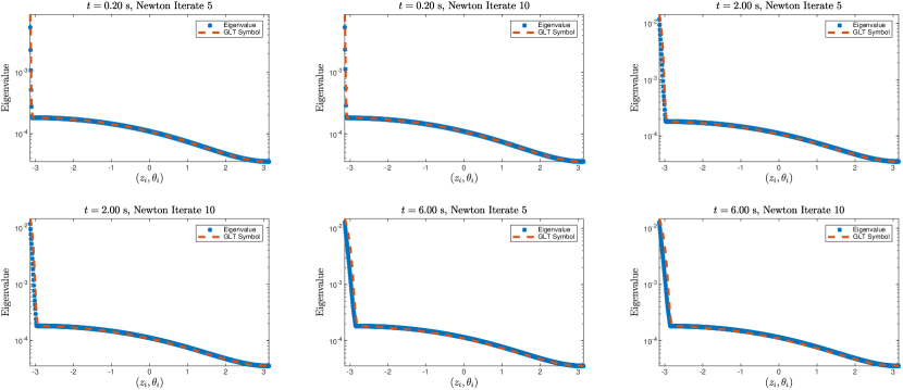
Figure 7: Arithmetic average. Comparison of the eigenvalues and spectral symbol for the coefficients in (17) with $h_{z}=40/(N-1)$, $\Delta t=0.1$, and $N=800$ on different time steps and for different iterates of the full Newton method.

As we observe, even for a small grid size thus namely far away from the asymptotic regime, there is a good matching between the predicted eigenvalues and the computed ones.

We consider the same test problem also for the case in which we use the upstream-weighted mean of the values of $K$ in (3). Again the result proved in Theorem C.3 is clearly depicted in Figure 8, in which we observe a good accordance between the spectral symbol and the computed eigenvalues already at coarse grid.

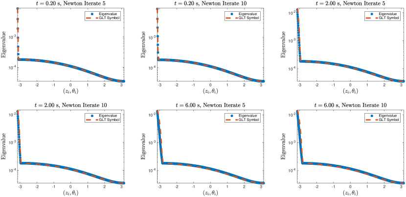
Figure 8: Upstream-weighted average. Comparison of the eigenvalues and spectral symbol for the coefficients in (17) with $h_{z}=40/(N-1)$, $\Delta t=0.1$, and $N=800$ on different time steps and for different iterates of the full Newton method.

To have a comparison in between the approximate and full sequence we consider also the only preconditioner we can apply on both sequence, namely the AS preconditioner, and compare the average number of iteration across the time steps in the weak scaling regime described in Section 6.2. From the results in Table 2 we observe readily that the spectrally equivalent sequence clearly catches the properties we are interested in.

$n_{p}$	Original sequence	Approximating sequence
1	212	212
4	267	267
16	277	285
64	296	296
256	217	217
1024	296	296

Table 2: Weak scaling. Comparison of the (rounded) average number of linear iteration employed by the AS preconditioner when built directly on the original sequence and when built on the approximating sequence obtained from the spectral analysis.

Appendix F Weak scalability

In this section we complement the results discussed in Section 6.2 by considering further details on the weak-scalability analysis.

In first place, we want to investigate numerically the consequences of Theorem 4.15. Indeed, from the theoretical analysis we expect that if we would use just the discretization of the diffusive part of the equation, then a cluster of eigenvalues at $1$ would appear and suggest good performances for the underlying Krylov solver. Since this is not feasible, we resorted to using either the multigrid hierarchies to further approximate the diffusive part. Therefore, we investigate here numerically the capability of such approximating sequence with respect to the original one. To have an homogeneous situation with respect to the coarse grid, and diminish the number of variables that could change the interpretation of the result, we resort to using just 30 iterations of a Block-Jacobi method with the ILU(0) factorization as a coarse solver.

	Avg. Nl.		Avg. L. It.s
$n_{p}$	It.s	N Jac.s		R
1	3	12	58	57
4	3	12	69	69
16	3	12	68	68
64	3	12	57	59
256	3	12	56	58
1024	3	12	57	57
4096	3	12	56	56

(a) VDSVMB

	Avg. Nl.		Avg. L. It.s
$n_{p}$	It.s	N Jac.s		R
1	3	11	82	83
4	3	12	87	73
16	3	12	83	75
64	3	12	79	87
256	3	12	77	82
1024	3	12	75	75
4096	3	12	73	77

(b) VSMATCH

Table 3: Algorithmic scalability for the Richards test problem. The average number of linear iteration per Newton iteration is computed taking the average of the ratio of linear iteration per Newton step across the time steps.

From the results collected in Table 3, we observe that both the multigrid strategies do manage in keeping the number of linear iteration more stable and smaller than the one-level AS preconditioner. This makes for an empirical confirmation of the two facts we want to ascertain. On one hand the spectral information of the matrix sequence $\{J_{\mathbf{N}}\}_{\mathbf{N}}$ are confirmed to be captured by the symmetric approximation, secondly, the multigrid hierarchies give a reliable approximation of the effect of inverting the theoretically implied sequence.

F.1 Finer details on the build and solve phases

To deepen the analysis, we look with a finer degree of detail at the performances of every slices of the bar-plots in Figure 6. Let us start from the bottom and look at the build phase of the Jacobian matrices; Figure 9. Up to $4096$ cores the assembly phase stays around the 70% of efficiency, and is only sligthly diminished to around the 60% on $8192$ cores.

Figure 9: Weak scaling. Speedup (left) and scaled efficiency (right) for setup of the Jacobian matrices.

Indeed, even if we are using a method that needs to assembly the matrices for building the preconditioners, we observe that this doesn’t hampers the overall efficiency of the method. This is even more true if we also consider the efficiency of the function evaluation routine (that is instead implemented in a matrix-free way) given in Figure 10. We notice that this mimics the overall efficiency of the whole procedure.

Figure 10: Weak scaling. Speedup (left) and scaled efficiency (right) for the evaluation of the $\boldsymbol{\Phi}$ function.

As it usually happens in nonlinear processes, what characterizes the overall performance is indeed the number and efficiency of the function evaluation calls. That, as we see from Table 4, are very stable with respect to the number of employed cores when the VSMATCH preconditioner is used for Newton correction, while shows some oscillations for the other preconditioners.

	VDSVBM		VSMATCH		AS
$n_{p}$	N Jac.s	NLin It.s	N Jac.s	NLin It.s	N Jac.s	NLin It.s
1	3	37	3	36	3	40
4	3	38	3	38	3	36
16	3	38	3	38	3	40
64	3	37	3	38	4	37
256	3	37	3	38	4	39
1024	3	39	3	38	4	41
4096	3	41	3	38	4	47
8192	3	40	3	38	4	48

Table 4: Weak scaling. Number of nonlinear iterations (NLin It.s), and number of computed Jacobians (N Jac.s) for the three preconditioners.

Finally, let us look further into the scalability performances of the solution of the linear systems associated with the Newton correction. In our strategy this is divided into three separate phases. A complete setup in which we build the hierarchies for the first time, an update phase in which we recompute just the smoothers when there has been a change in the Jacobian, and the application phase inside the Krylov iterative method. For what concern the first two phases, Figures 11a, 11b show that the update strategy reduces effectively the time needed to prepare the preconditioner, while keeping a reasonable quality for the aggregation procedure.

(a) VDSVMB Setup calls.

(b) VSMATCH Setup calls.

Figure 11: Weak scaling. Setup phases of the preconditioners in which subsequent calls are updates.

In order to better understand the results on the execution time per iteration of the AMG preconditioners discussed in the paper, we also report (average) operator complexity of the two different methods. We recall that the operator complexity of an AMG method is defined as

$$\text{opc}=\frac{\sum_{l=0}^{\text{nl}-1}\operatorname{nnz}(A_{l})}{\operatorname{nnz}(A_{0})}>1,$$

and is usually both a measure of memory occupancy and of the time complexity for the method application in a V-cycle⁷.

(a) Average operator complexity

(b) Average time $T(s)$ for linear solver (left) and scaled efficiency (right)

Figure 12: Weak scaling. Average operator complexity of AMG preconditioners and average time $T(s)$ for linear solver.

Looking also at the overall behavior of the solving times is useful. If we compare the results in Figure 12b with the ones in Figure 5b, we observe that the efficiency for the linear system solve phase reflects the global efficiency and is not hampered by the fact that we are building Jacobians and auxiliary matrices, see again Figure 9, or by the way in which we are performing the function evaluations.

References

- 1 Farthing MW, and Ogden FL. Numerical Solution of Richards’ Equation: A Review of Advances and Challenges. Soil Sci Soc Am J. 2017;81(6):1257–1269. Available from: https://acsess.onlinelibrary.wiley.com/doi/abs/10.2136/sssaj2017.02.0058.
- 2 van Genuchten MT. A Closed-form Equation for Predicting the Hydraulic Conductivity of Unsaturated Soils. Soil Sci Soc Am J. 1980;44(5):892–898. Available from: https://acsess.onlinelibrary.wiley.com/doi/abs/10.2136/sssaj1980.03615995004400050002x.
- 3 Celia MA, Bouloutas ET, and Zarba RL. A general mass-conservative numerical solution for the unsaturated flow equation. Water Resources Research. 1990;26(7):1483–1496. Available from: https://agupubs.onlinelibrary.wiley.com/doi/abs/10.1029/WR026i007p01483.
- 4 Miller CT, Williams GA, Kelley CT, and Tocci MD. Robust solution of Richards’ equation for nonuniform porous media. Water Resources Research. 1998;34(10):2599–2610. Available from: https://agupubs.onlinelibrary.wiley.com/doi/abs/10.1029/98WR01673.
- 5 Jones JE, and Woodward CS. Newton–Krylov-multigrid solvers for large-scale, highly heterogeneous, variably saturated flow problems. Advances in Water Resources. 2001;24(7):763–774. Available from: http://www.sciencedirect.com/science/article/pii/S0309170800000750.
- 6 Hindmarsh AC, Brown PN, Grant KE, Lee SL, Serban R, Shumaker DE, et al. SUNDIALS: Suite of nonlinear and differential/algebraic equation solvers. ACM Transactions on Mathematical Software (TOMS). 2005;31(3):363–396.
- 7 D’Ambra P, Durastante F, and Filippone S. AMG preconditioners for Linear Solvers at Extreme Scale. SIAM J on Sci Comp. 2021;43(5).
- 8 Brooks RH, and Corey AT. Hydraulic properties of porous media. Hydrology papers (Colorado State University); no 3. 1964;.
- 9 Szymkiewicz A. Approximation of internodal conductivities in numerical simulation of one-dimensional infiltration, drainage, and capillary rise in unsaturated soils. Water Resources Research. 2009;45(10). Available from: https://agupubs.onlinelibrary.wiley.com/doi/abs/10.1029/2008WR007654.
- 10 Baker DL. General Validity of Conductivity Means in Unsaturated Flow Models. Journal of Hydrologic Engineering. 2006;11(6):526–538.
- 11 Haverkamp R, and Vauclin M. A note on estimating finite difference interblock hydraulic conductivity values for transient unsaturated flow problems. Water Resources Research. 1979;15(1):181–187. Available from: https://agupubs.onlinelibrary.wiley.com/doi/abs/10.1029/WR015i001p00181.
- 12 Oldenburg CM, and Pruess K. On numerical modeling of capillary barriers. Water Resources Research. 1993;29(4):1045–1056. Available from: https://agupubs.onlinelibrary.wiley.com/doi/abs/10.1029/92WR02875.
- 13 Srivastava R, and Guzman-Guzman A. Analysis of hydraulic conductivity averaging schemes for one-dimensional steady-state unsaturated flow. Ground Water. 1995 2020/9/29/;33:946+. 6.
- 14 Garoni C, and Serra-Capizzano S. Generalized Locally Toeplitz Sequences: Theory and Applications: Volume I. Cham: Springer International Publishing; 2017. Available from: https://doi.org/10.1007/978-3-319-53679-8.
- 15 Garoni C, and Serra-Capizzano S. Generalized locally Toeplitz sequences: theory and applications. Vol. II. Springer, Cham; 2018. Available from: https://doi.org/10.1007/978-3-030-02233-4.
- 16 Kollet SJ, and Maxwell RM. Integrated Surface-groundwater Flow Modeling: a Free-surface Overland Flow Boundary Condition in a Parallel Groundwater Flow Model. Advances in Water Resources. 2005 4;29(7). Available from: https://www.osti.gov/biblio/887270.
- 17 Maxwell RM. A terrain-following grid transform and preconditioner for parallel, large-scale, integrated hydrologic modeling. Advances in Water Resources. 2013 Mar;53:109–117.
- 18 Filippone S, and Colajanni M. PSBLAS: a library for parallel linear algebra computations on sparse matrices. ACM TOMS. 2000 Dec;26(4):527–550.
- 19 Filippone S, and Buttari A. Object-Oriented Techniques for Sparse Matrix Computations in Fortran 2003. ACM TOMS. 2012;38(4):23:1–23:20.
- 20 Buttari A, D’Ambra P, di Serafino D, and Filippone S. 2LEV-D2P4: a package of high-performance preconditioners for scientific and engineering applications. Appl Algebra Engrg Comm Comput. 2007;18(3):223–239.
- 21 D’Ambra P, di Serafino D, and Filippone S. MLD2P4: a package of parallel algebraic multilevel domain decomposition preconditioners in Fortran 95. ACM Trans Math Software. 2010;37(3):Art. 30, 23.
- 22 Vaněk P, Mandel J, and Brezina M. Algebraic multigrid by smoothed aggregation for second and fourth order elliptic problems. Computing. 1996;56(3):179–196. International GAMM-Workshop on Multi-level Methods (Meisdorf, 1994).
- 23 D’Ambra P, and Vassilevski PS. Adaptive AMG with coarsening based on compatible weighted matching. Comput Vis Sci. 2013;16(2):59–76.
- 24 D’Ambra P, Filippone S, and Vassilevski PS. BootCMatch: A Software Package for Bootstrap AMG Based on Graph Weighted Matching. ACM Trans Math Softw. 2018 Jun;44(4). Available from: https://doi.org/10.1145/3190647.
- 25 D’Ambra P, and Filippone S. A parallel generalized relaxation method for high-performance image segmentation on GPUs. J Comput Appl Math. 2016;293:35–44.
- 26 Maxwell RM, Condon LE, Smith SG, Woodward CS, Falgout RD, Ferguson IM, et al.; Integrated GroundWater Modeling Center Report. ParFlow User’s Manual. Zenodo. 2022;p. 171. Available from: https://github.com/parflow/parflow/blob/master/parflow-manual.pdf.
- 27 Haverkamp R, Vauclin M, Touma J, Wierenga PJ, and Vachaud G. A Comparison of Numerical Simulation Models For One-Dimensional Infiltration. Soil Science Society of America Journal. 1977;41(2):285–294. Available from: https://acsess.onlinelibrary.wiley.com/doi/abs/10.2136/sssaj1977.03615995004100020024x.