Discord and Decoherence

Abstract

In quantum information theory, quantum discord has been proposed as a tool to characterise the presence of “quantum correlations” between the subparts of a given system. Whether a system behaves quantum-mechanically or classically is believed to be impacted by the phenomenon of decoherence, which originates from the unavoidable interaction between this system and an environment. Generically, decoherence is associated with a decrease of the state purity, i.e. a transition from a pure to a mixed state. In this paper, we investigate how quantum discord is modified by this quantum-to-classical transition. This study is carried out on systems described by quadratic Hamiltonians and Gaussian states, with generalised squeezing parameters. A generic parametrisation is also introduced to describe the way the system is partitioned into two subsystems. We find that the evolution of quantum discord in presence of an environment is a competition between the growth of the squeezing amplitude and the decrease of the state purity. In phase space, this corresponds to whether the semi-minor axis of the Wigner ellipse increases or decreases, which has a clear geometrical interpretation. Finally, these considerations are applied to primordial cosmological perturbations, where we find that quantum discord can remain large even in the presence of strong decoherence.

1 Introduction

A intriguing fact in modern science is that, sometimes, it is not straightforward to decide whether a system behaves classically or quantum-mechanically. This is for instance the case in Cosmology where it is believed that the structures observed in our universe are nothing but quantum fluctuations amplified to astrophysical scales [1, 2, 3]. Even if this hypothesis allows us to explain the properties of these structures, acquiring evidence that would establish their origin beyond any doubt turns out to be highly non-trivial. Indeed, assuming that the primordial fluctuations are stochastic rather than quantum leads to almost the same consequences up to corrections that, in practice, are very difficult to reveal experimentally [4, 5].

Recently, new methods have been developed to address the question of whether a system is classical or quantum-mechanical. A typical approach consists in dividing the system into two sub-systems and to study and characterise the nature of the correlations between these two sub-systems. As a matter of fact, there exist efficient tools to decide whether correlations are classical or quantum-mechanical in nature. Sometimes, indeed, correlations are impossible to understand in a classical framework (see, for instance, the Bell experiments [6, 7]) which establishes unambiguously their quantum origin. This strategy leads to the concept of quantum discord [8, 9]. However, the ability of quantum discord to precisely identify the quantum nature of some correlations has been challenged in the case of mixed states while, in the case of pure states, there is a one-to-one correspondence between quantum discord and entropy of entanglement [10, 11]. On the other hand, the quantum-to-classical transition of a system is generically believed to be connected to the phenomenon of decoherence [12, 13]. This mechanism, which has been observed in the laboratory [7], takes into account that any system is in fact always an open system, namely a system in interaction with other degrees of freedom that collectively constitute an environment. This interaction, when one is only interested in the properties of the system, is responsible for the appearance of classical properties.

It is therefore interesting to study how the quantum discord “responds” to the presence of decoherence in a system and to investigate how quantum discord can track the “classicalization” of a system. This is the main goal of the present paper. This study will be carried out in the generic case of a quadratic Hamiltonian. Physically, this is very relevant since many systems are described by this type of Hamiltonians. This is for instance the case for the Schwinger effect, the dynamical Casimir effect, the Hawking effect, inflationary fluctuations, etc. Technically, this is advantageous since the quantisation of these systems always leads to Gaussian states for which there exists an efficient formalism permitting the calculation of quantum discord. When it comes to concrete applications, we will consider the example of cosmological perturbations [14]. In addition to the advantages mentioned above, this will also allow us to shed new light on the question of whether their quantum origin can be observationally revealed, a long-standing question in Cosmology that has recently been the subject of many new studies [4, 15, 16, 17, 18, 19, 20, 21, 22, 23].

This article is organised as follows. In Sec. 2, we present a description of the quadratic systems considered in this paper and provide the formulas permitting the calculation of their quantum discord. In Sec. 3, as a warm-up, we explain how the time evolution of these systems and their quantum discord can be calculated in absence of an environment. In Sec. 4, we introduce a simple model, based on the Caldeira-Leggett model, which allows us to study and calculate quantum discord in presence of decoherence. In Sec. 5, we apply this formalism to the theory of cosmological perturbations of quantum-mechanical origin. At the end of the article, in Sec. 6, we present our conclusions. Finally, the technical details of our calculations are given in a series of appendices. In Sec. A, we come back to the notion of partitions of a system and explain it in more details. In Sec. B, we calculate the covariance matrix of a Gaussian system for an arbitrary partition. In Sec. C, we explain how the formula giving the quantum discord used in the main text is arrived at. In Sec. D, we calculate the covariance matrix of the system in presence of an environment and derive efficient approximations for its components.

2 Quantum discord of a Gaussian field

2.1 Quantum phase space

In this work we consider the case of a real quantum scalar field with a local quadratic Hamiltonian

$$\hat{H}=\frac{1}{2}\int_{\mathbb{R}^{3}}\mathrm{d}^{3}\bm{x}\,\hat{z}^{\mathrm{T}}(\bm{x})\Lambda(\tau)\hat{z}(\bm{x})\,,$$ (2.1)

where $\hat{z}(\bm{x})=\left(\hat{\phi}(\bm{x})\,,\hat{\pi}_{\phi}(\bm{x})\right)^{\mathrm{T}}$ contains the field $\hat{\phi}$ and its conjugate momentum $\hat{\pi}_{\phi}$, which satisfy the canonical commutation relations

$$\left[\hat{\phi}(\bm{x}),\hat{\pi}_{\phi}(\bm{y})\right]=i\delta(\bm{x}-\bm{y}).$$ (2.2)

We assume that the $2$$\times$$2$ symmetric matrix $\Lambda(\tau)$ does not depend on $\bm{x}$ but only on time $\tau$, which can result from the invariance under spatial translations of the physical setup on which the field is introduced. For instance, the field $\phi$ may describe cosmological perturbations evolving on top of a homogeneous and isotropic background, as further discussed in Sec. 5, but for now the formalism we develop remains generic and applies to any system described by a (possibly infinite) collection of parametric oscillators. Note that $\Lambda_{\phi\phi}(\tau)$ can nonetheless contain gradient operators $\partial/\partial\bm{x}$ to any positive (in agreement with the locality assumption) and even (in order to preserve homogeneity and isotropy) power. If the theory does not feature higher-than two derivatives, which we assume here, then the other entries of ${\Lambda}$ cannot contain spatial gradients. In what follows we introduce several successive canonical transformation, i.e. changes of variables that preserve the structure of the commutators (2.2), which make the expression of the Hamiltonian (2.1) simpler.

Let us perform a first canonical transformation and introduce the variables $\hat{v}(\bm{x})$ and $\hat{p}(\bm{x})$ defined as

$$\begin{split}\hat{\phi}(\bm{x})&=\mathchoice{{\hbox{$\displaystyle\sqrt{\Lambda_{\pi\pi}\,}$}\lower 0.4pt\hbox{\vrule height=6.83331pt,depth=-5.46667pt}}}{{\hbox{$\textstyle\sqrt{\Lambda_{\pi\pi}\,}$}\lower 0.4pt\hbox{\vrule height=6.83331pt,depth=-5.46667pt}}}{{\hbox{$\scriptstyle\sqrt{\Lambda_{\pi\pi}\,}$}\lower 0.4pt\hbox{\vrule height=4.78333pt,depth=-3.82668pt}}}{{\hbox{$\scriptscriptstyle\sqrt{\Lambda_{\pi\pi}\,}$}\lower 0.4pt\hbox{\vrule height=3.41666pt,depth=-2.73334pt}}}\hat{v}(\bm{x})\,\\ \hat{\pi}_{\phi}(\bm{x})&=\left(\frac{1}{2}\frac{{\Lambda}^{\prime}_{\pi\pi}}{\Lambda_{\pi\pi}}-\Lambda_{\phi\pi}\right)\frac{\hat{v}(\bm{x})}{\mathchoice{{\hbox{$\displaystyle\sqrt{\Lambda_{\pi\pi}\,}$}\lower 0.4pt\hbox{\vrule height=6.83331pt,depth=-5.46667pt}}}{{\hbox{$\textstyle\sqrt{\Lambda_{\pi\pi}\,}$}\lower 0.4pt\hbox{\vrule height=6.83331pt,depth=-5.46667pt}}}{{\hbox{$\scriptstyle\sqrt{\Lambda_{\pi\pi}\,}$}\lower 0.4pt\hbox{\vrule height=4.78333pt,depth=-3.82668pt}}}{{\hbox{$\scriptscriptstyle\sqrt{\Lambda_{\pi\pi}\,}$}\lower 0.4pt\hbox{\vrule height=3.41666pt,depth=-2.73334pt}}}}+\frac{\hat{p}(\bm{x})}{\mathchoice{{\hbox{$\displaystyle\sqrt{\Lambda_{\pi\pi}\,}$}\lower 0.4pt\hbox{\vrule height=6.83331pt,depth=-5.46667pt}}}{{\hbox{$\textstyle\sqrt{\Lambda_{\pi\pi}\,}$}\lower 0.4pt\hbox{\vrule height=6.83331pt,depth=-5.46667pt}}}{{\hbox{$\scriptstyle\sqrt{\Lambda_{\pi\pi}\,}$}\lower 0.4pt\hbox{\vrule height=4.78333pt,depth=-3.82668pt}}}{{\hbox{$\scriptscriptstyle\sqrt{\Lambda_{\pi\pi}\,}$}\lower 0.4pt\hbox{\vrule height=3.41666pt,depth=-2.73334pt}}}}\,,\end{split}$$ (2.3)

where a prime denotes derivation with respect to time, and where one can easily check that $\hat{v}$ and $\hat{p}$ obey the same commutation relations as the original fields, see Eq. (2.2). In terms of these new variables, the Hamiltonian takes the simple form [24]

$$\hat{H}=\frac{1}{2}\int_{\mathbb{R}^{3}}\mathrm{d}^{3}\bm{x}\left[\hat{p}^{2}(\bm{x})+\omega^{2}\hat{v}^{2}(\bm{x})\right]\,,$$ (2.4)

where $\omega^{2}=\Lambda_{\phi\phi}\Lambda_{\pi\pi}+1/2({\Lambda}^{\prime\prime}_{\pi\pi}/\Lambda_{\pi\pi})-3/4({\Lambda}^{\prime}_{\pi\pi}/\Lambda_{\pi\pi})^{2}-{\Lambda}^{\prime}_{\phi\pi}-\Lambda_{\phi\pi}^{2}+\Lambda_{\phi\pi}{\Lambda}^{\prime}_{\pi\pi}/\Lambda_{\pi\pi}$ encodes all the information about the dynamics.

We then perform a second canonical transformation, in the form of the Fourier expansion

$$\hat{v}(\bm{x})=\frac{1}{\left(2\pi\right)^{3/2}}\int_{\mathbb{R}^{3}}\mathrm{d}^{3}\bm{k}\,e^{-i\bm{k}\cdot\bm{x}}\hat{v}_{\bm{k}}$$ (2.5)

and a similar expression for $\hat{p}(\bm{x})$. The fact that this defines a canonical transformation can be easily seen from combining the inverse Fourier transform, $\hat{v}_{\bm{k}}=(2\pi)^{-3/2}\int\mathrm{d}^{3}\bm{x}\,e^{i\bm{k}\cdot\bm{x}}\hat{v}(\bm{x})$ (and a similar expression for $\hat{p}_{\bm{k}}$) with Eq. (2.2) for the fields $\hat{v}(\bm{x})$ and $\hat{p}(\bm{x})$, which yields

$$\left[\hat{v}_{\bm{k}},\hat{p}_{\bm{k}^{\prime}}^{\dagger}\right]=i\delta(\bm{k}-\bm{k}^{\prime})\,,$$ (2.6)

while $[\hat{v}_{\bm{k}},\hat{v}_{\bm{k}^{\prime}}^{\dagger}]=[\hat{p}_{\bm{k}},\hat{p}_{\bm{k}^{\prime}}^{\dagger}]=0$. Plugging the Fourier expansions into the Hamiltonian (2.4), one obtains

$$\hat{H}=\int_{\mathbb{R}^{3+}}\mathrm{d}^{3}\bm{k}\,\hat{\mathcal{H}}_{\bm{k}}=\int_{\mathbb{R}^{3+}}\mathrm{d}^{3}\bm{k}\left[\hat{p}_{\bm{k}}\hat{p}_{\bm{k}}^{\dagger}+\omega^{2}\left(k,t\right)\hat{v}_{\bm{k}}\hat{v}_{\bm{k}}^{\dagger}\right],$$ (2.7)

which defines the Hamiltonian density in Fourier space $\hat{\mathcal{H}}_{\bm{k}}$. In this expression, $\omega$ can depend on $k$ since, as pointed out above, it may involve the gradient operator. It is important to notice that the operators $\hat{v}_{\bm{k}}$ and $\hat{p}_{{\bm{k}}}$ are not Hermitian. Indeed, since $\hat{v}(t,{\bm{x}})$ is real, one has $\hat{v}_{\bm{k}}^{\dagger}=\hat{v}_{-\bm{k}}$ and a similar relation for the conjugate momentum. This shows that independent degrees of freedom are labelled by half the Fourier space only, and explains why the integral is performed over $\mathbb{R}^{3+}=\mathbb{R}^{2}\times\mathbb{R}^{+}$ in Eq. (2.7). In the helicity basis, this also allows one to decompose the fields $\hat{v}_{\bm{k}}$ and $\hat{p}_{{\bm{k}}}$ onto creation and annihilation operators as

$$\hat{v}_{\bm{k}}=\frac{1}{\mathchoice{{\hbox{$\displaystyle\sqrt{2k\,}$}\lower 0.4pt\hbox{\vrule height=6.94444pt,depth=-5.55559pt}}}{{\hbox{$\textstyle\sqrt{2k\,}$}\lower 0.4pt\hbox{\vrule height=6.94444pt,depth=-5.55559pt}}}{{\hbox{$\scriptstyle\sqrt{2k\,}$}\lower 0.4pt\hbox{\vrule height=4.8611pt,depth=-3.8889pt}}}{{\hbox{$\scriptscriptstyle\sqrt{2k\,}$}\lower 0.4pt\hbox{\vrule height=3.47221pt,depth=-2.77779pt}}}}\left(\hat{c}_{\bm{k}}+\hat{c}_{-\bm{k}}^{\dagger}\right)\qquad\text{and}\qquad\hat{p}_{\bm{k}}=-i\mathchoice{{\hbox{$\displaystyle\sqrt{\frac{k}{2}\,}$}\lower 0.4pt\hbox{\vrule height=10.16666pt,depth=-8.13336pt}}}{{\hbox{$\textstyle\sqrt{\frac{k}{2}\,}$}\lower 0.4pt\hbox{\vrule height=7.11665pt,depth=-5.69336pt}}}{{\hbox{$\scriptstyle\sqrt{\frac{k}{2}\,}$}\lower 0.4pt\hbox{\vrule height=5.08331pt,depth=-4.06668pt}}}{{\hbox{$\scriptscriptstyle\sqrt{\frac{k}{2}\,}$}\lower 0.4pt\hbox{\vrule height=5.08331pt,depth=-4.06668pt}}}\left(\hat{c}_{\bm{k}}-\hat{c}_{-\bm{k}}^{\dagger}\right),$$ (2.8)

where $\hat{c}_{\bm{k}}$ and $\hat{c}_{\bm{k}^{\prime}}^{\dagger}$ obey the commutation relation $[\hat{c}_{\bm{k}},\hat{c}_{\bm{k}^{\prime}}^{\dagger}]=\delta(\bm{k}-\bm{k}^{\prime})$. By plugging the above into Eq. (2.7), one obtains

$$\hat{H}= \int_{\mathbb{R}^{3+}}\mathrm{d}^{3}\bm{k}\biggl{[}\frac{k}{2}\left(\frac{\omega^{2}}{k^{2}}+1\right)\left(\hat{c}_{\bm{k}}\hat{c}_{\bm{k}}^{\dagger}+\hat{c}_{-\bm{k}}^{\dagger}\hat{c}_{-\bm{k}}\right)+\frac{k}{2}\left(\frac{\omega^{2}}{k^{2}}-1\right)\left(\hat{c}_{\bm{k}}\hat{c}_{-\bm{k}}+\hat{c}_{-\bm{k}}^{\dagger}\hat{c}_{\bm{k}}^{\dagger}\right)\biggr{]}.$$ (2.9)

In this expression, the first term does not lead to net particle creation and represents a collection of free oscillators while the second term either creates or destroys a pair of particles with momenta $\bm{k}$ and $-\bm{k}$, and can be seen as resulting from the interaction with an exterior classical source. Note that the four combinations of ladder operators appearing in Eq. (2.9) are the only quadratic terms that are allowed by statistical isotropy, i.e. they are the only combinations that ensure momentum conservation in the particle content. Let us also notice that the form (2.9) is not the one commonly used in Cosmology [which is given by Eq. (14) of Ref. [5]]. However, it is related to it by a simple canonical transformation and is, therefore, equivalent to it.

Since $\hat{v}_{\bm{k}}$ and $\hat{p}_{{\bm{k}}}$ are not Hermitian, it is convenient to perform a third and last canonical transformation, and introduce the Hermitian operators corresponding to the Hermitian and anti-Hermitian parts of $\hat{v}_{\bm{k}}$ and $\hat{p}_{\bm{k}}$,

$$\hat{v}_{\bm{k}}^{\mathrm{R}}=\frac{\hat{v}_{\bm{k}}+\hat{v}_{\bm{k}}^{\dagger}}{\mathchoice{{\hbox{$\displaystyle\sqrt{2\,}$}\lower 0.4pt\hbox{\vrule height=6.44444pt,depth=-5.15558pt}}}{{\hbox{$\textstyle\sqrt{2\,}$}\lower 0.4pt\hbox{\vrule height=6.44444pt,depth=-5.15558pt}}}{{\hbox{$\scriptstyle\sqrt{2\,}$}\lower 0.4pt\hbox{\vrule height=4.51111pt,depth=-3.6089pt}}}{{\hbox{$\scriptscriptstyle\sqrt{2\,}$}\lower 0.4pt\hbox{\vrule height=3.22221pt,depth=-2.57779pt}}}}\,,\qquad\hat{v}_{\bm{k}}^{\mathrm{I}}=\frac{\hat{v}_{\bm{k}}-\hat{v}_{\bm{k}}^{\dagger}}{\mathchoice{{\hbox{$\displaystyle\sqrt{2\,}$}\lower 0.4pt\hbox{\vrule height=6.44444pt,depth=-5.15558pt}}}{{\hbox{$\textstyle\sqrt{2\,}$}\lower 0.4pt\hbox{\vrule height=6.44444pt,depth=-5.15558pt}}}{{\hbox{$\scriptstyle\sqrt{2\,}$}\lower 0.4pt\hbox{\vrule height=4.51111pt,depth=-3.6089pt}}}{{\hbox{$\scriptscriptstyle\sqrt{2\,}$}\lower 0.4pt\hbox{\vrule height=3.22221pt,depth=-2.57779pt}}}i}\,,\qquad\hat{p}_{\bm{k}}^{\mathrm{R}}=\frac{\hat{p}_{\bm{k}}+\hat{p}_{\bm{k}}^{\dagger}}{\mathchoice{{\hbox{$\displaystyle\sqrt{2\,}$}\lower 0.4pt\hbox{\vrule height=6.44444pt,depth=-5.15558pt}}}{{\hbox{$\textstyle\sqrt{2\,}$}\lower 0.4pt\hbox{\vrule height=6.44444pt,depth=-5.15558pt}}}{{\hbox{$\scriptstyle\sqrt{2\,}$}\lower 0.4pt\hbox{\vrule height=4.51111pt,depth=-3.6089pt}}}{{\hbox{$\scriptscriptstyle\sqrt{2\,}$}\lower 0.4pt\hbox{\vrule height=3.22221pt,depth=-2.57779pt}}}}\,,\qquad\hat{p}_{\bm{k}}^{\mathrm{I}}=\frac{\hat{p}_{\bm{k}}-\hat{p}_{\bm{k}}^{\dagger}}{\mathchoice{{\hbox{$\displaystyle\sqrt{2\,}$}\lower 0.4pt\hbox{\vrule height=6.44444pt,depth=-5.15558pt}}}{{\hbox{$\textstyle\sqrt{2\,}$}\lower 0.4pt\hbox{\vrule height=6.44444pt,depth=-5.15558pt}}}{{\hbox{$\scriptstyle\sqrt{2\,}$}\lower 0.4pt\hbox{\vrule height=4.51111pt,depth=-3.6089pt}}}{{\hbox{$\scriptscriptstyle\sqrt{2\,}$}\lower 0.4pt\hbox{\vrule height=3.22221pt,depth=-2.57779pt}}}i}\,.$$ (2.10)

The transformation (2.10) can be inverted according to $\hat{v}_{\bm{k}}=\left(\hat{v}_{\bm{k}}^{\mathrm{R}}+i\hat{v}_{\bm{k}}^{\mathrm{I}}\right)/\mathchoice{{\hbox{$\displaystyle\sqrt{2\,}$}\lower 0.4pt\hbox{\vrule height=6.44444pt,depth=-5.15558pt}}}{{\hbox{$\textstyle\sqrt{2\,}$}\lower 0.4pt\hbox{\vrule height=6.44444pt,depth=-5.15558pt}}}{{\hbox{$\scriptstyle\sqrt{2\,}$}\lower 0.4pt\hbox{\vrule height=4.51111pt,depth=-3.6089pt}}}{{\hbox{$\scriptscriptstyle\sqrt{2\,}$}\lower 0.4pt\hbox{\vrule height=3.22221pt,depth=-2.57779pt}}}$ and $\hat{p}_{\bm{k}}=\left(\hat{p}_{\bm{k}}^{\mathrm{R}}+i\hat{p}_{\bm{k}}^{\mathrm{I}}\right)/\mathchoice{{\hbox{$\displaystyle\sqrt{2\,}$}\lower 0.4pt\hbox{\vrule height=6.44444pt,depth=-5.15558pt}}}{{\hbox{$\textstyle\sqrt{2\,}$}\lower 0.4pt\hbox{\vrule height=6.44444pt,depth=-5.15558pt}}}{{\hbox{$\scriptstyle\sqrt{2\,}$}\lower 0.4pt\hbox{\vrule height=4.51111pt,depth=-3.6089pt}}}{{\hbox{$\scriptscriptstyle\sqrt{2\,}$}\lower 0.4pt\hbox{\vrule height=3.22221pt,depth=-2.57779pt}}}$, and one can readily check that these relations define a canonical transformation, namely that $[\hat{v}_{\bm{k}}^{s},\hat{p}_{\bm{k}^{\prime}}^{s^{\prime}}]=i\delta(\bm{k}-\bm{k}^{\prime})\delta_{s,s^{\prime}}$ and that $[\hat{v}_{\bm{k}}^{s},\hat{v}_{\bm{k}^{\prime}}^{s^{\prime}}]=[\hat{p}_{\bm{k}}^{s},\hat{p}_{\bm{k}^{\prime}}^{s^{\prime}}]=0$ where $s=\mathrm{R},\mathrm{I}$. It is also clear from these expressions that $\hat{v}_{\bm{k}}^{s}$ and $\hat{p}_{\bm{k}}^{s}$ are Hermitian operators, and that the Hamiltonian reads

$$\hat{H} =\int_{\mathbb{R}^{3+}}\mathrm{d}^{3}\bm{k}\sum_{s=\mathrm{R,I}}\hat{\mathcal{H}}_{\bm{k}}^{s}=\frac{1}{2}\int_{\mathbb{R}^{3+}}\mathrm{d}^{3}\bm{k}\sum_{s=\mathrm{R,I}}\left[(\hat{p}_{\bm{k}}^{s})^{2}+\omega^{2}(k,\tau)(\hat{v}_{\bm{k}}^{s})^{2}\right]\,.$$ (2.11)

The advantage of this last parameterisation is that it makes the Hamiltonian sum separable, see Eq. (2.11). In other words, it describes a collection of independent parametric oscillators. If the initial quantum state is factorisable in that basis, which is for instance the case for the vacuum state selected by that Hamiltonian, it remains so at later time, and the dynamical evolution does not generate correlation or entanglement between different subspaces.

2.2 Partitions

As mentioned above, the system under consideration can be factorised into independent Fourier subspaces, within which entangled pairs of particles with opposite wave-momenta are created. Our goal is to measure the amount of entanglement associated with this mechanism, and to determine whether the resulting correlations have genuinely quantum properties.

Experiments aimed at testing the quantum nature of a physical setup usually rely on probing the properties of the correlations between two of its subsystems. In Bell inequality experiments for instance, the correlations between the spin states of two entangled particles are tested against a possible local hidden-variables theory. In that case, the way the physical system is split into two subsystems is obvious: the two subsystems are simply the two space-like separated particles. One may choose to parameterise phase space by means of other combinations of the spin operators, but given that Bell experiments test for locality, it is clear that the two particles constitute a preferred partition.

The situation is however less clear for quantum fields. One may still choose to work in real space, and probe the nature of the correlations for two spatially-separated regions, see for instance Refs. [25, 21]. However, in this approach, one has to deal with mixed states, coming from the fact that when observing the field at two distinct locations in real space one implicitly traces over the configurations of the field in all other locations, making the reduced state of interest a mixed one. This problem does not occur in Fourier space since different Fourier subspaces are uncoupled. Since we want to study the effect of decoherence on the presence of quantum correlations, it seems important to first isolate the decoherence associated with the coupling to environmental degrees of freedom, from the one coming from the effective mixing effect mentioned above. This is why in this work we choose to study correlations within Fourier subspaces, leaving the combination of both mixing effects (i.e. the analysis of quantum discord in real space in the presence of an environment) for future work.

In Fourier space, there is no obvious way to split the system into two subsystems. At the technical level, this implies that the construction of Hermitian operators out of $\hat{v}_{\bm{k}}$ and $\hat{p}_{\bm{k}}$ is not unique, and that Eq. (2.10) is not the only possibility. For instance, one can consider the set of operators $\hat{q}_{\bm{k}}$ and $\hat{\pi}_{\bm{k}}$ involving ladder operators of a single mode $\bm{k}$ (and excluding $-\bm{k}$), namely [5]

$$\hat{q}_{\bm{k}} =\frac{1}{\mathchoice{{\hbox{$\displaystyle\sqrt{2k\,}$}\lower 0.4pt\hbox{\vrule height=6.94444pt,depth=-5.55559pt}}}{{\hbox{$\textstyle\sqrt{2k\,}$}\lower 0.4pt\hbox{\vrule height=6.94444pt,depth=-5.55559pt}}}{{\hbox{$\scriptstyle\sqrt{2k\,}$}\lower 0.4pt\hbox{\vrule height=4.8611pt,depth=-3.8889pt}}}{{\hbox{$\scriptscriptstyle\sqrt{2k\,}$}\lower 0.4pt\hbox{\vrule height=3.47221pt,depth=-2.77779pt}}}}\left(\hat{c}_{\bm{k}}+\hat{c}_{\bm{k}}^{\dagger}\right)\qquad\text{and}\qquad\hat{\pi}_{\bm{k}}=-i\mathchoice{{\hbox{$\displaystyle\sqrt{\frac{k}{2}\,}$}\lower 0.4pt\hbox{\vrule height=10.16666pt,depth=-8.13336pt}}}{{\hbox{$\textstyle\sqrt{\frac{k}{2}\,}$}\lower 0.4pt\hbox{\vrule height=7.11665pt,depth=-5.69336pt}}}{{\hbox{$\scriptstyle\sqrt{\frac{k}{2}\,}$}\lower 0.4pt\hbox{\vrule height=5.08331pt,depth=-4.06668pt}}}{{\hbox{$\scriptscriptstyle\sqrt{\frac{k}{2}\,}$}\lower 0.4pt\hbox{\vrule height=5.08331pt,depth=-4.06668pt}}}\left(\hat{c}_{\bm{k}}-\hat{c}_{\bm{k}}^{\dagger}\right),$$ (2.12)

which are indeed Hermitian and satisfy $[\hat{q}_{\bm{k}},\hat{\pi}_{{\bm{k}}^{\prime}}]=i\delta({\bm{k}}-{\bm{k}}^{\prime})$. The variables (2.10) and (2.12) define two partitions (namely a partition between the real and imaginary sector, and between the $\bm{k}$ and $-\bm{k}$ sector, respectively), and these two partitions feature different correlations of different amount and nature.

Since there is no preferred partition, a generic approach is to probe the nature of the correlations in all possible partitions. This is why we now define the notion of quantum partitions at a more formal level, and see how different partitions are related to each other (we refer the reader to Appendix A for a more detailed analysis of partitions). A partition of a Fourier subspace into two subsystems $1$ and $2$ is encoded in the phase-space vector

$$\hat{R}_{1/2}=\left(k^{1/2}\hat{q}_{\bm{k}}^{(1)},k^{-1/2}\hat{\pi}_{\bm{k}}^{(1)},k^{1/2}\hat{q}_{\bm{k}}^{(2)},k^{-1/2}\hat{\pi}_{\bm{k}}^{(2)}\right)^{\mathrm{T}}\,,$$ (2.13)

where the two first entries concern the first sector and the two last entries describe the second sector (the prefactors $k^{1/2}$ and $k^{-1/2}$ are introduced to make all entries of the $\hat{R}_{1/2}$ vector of the same dimension), and where the commutators between the entries of $\hat{R}_{1/2}$ are canonical (i.e. the only non-vanishing commutators are between the first and the second, and the third and the fourth, entries, and this commutator equals $i$). For instance, in the $\mathrm{R}/\mathrm{I}$ partition corresponding to Eq. (2.10), one has $\hat{R}_{\mathrm{R}/\mathrm{I}}=(k^{1/2}\hat{v}_{\bm{k}}^{\mathrm{R}},k^{-1/2}\hat{p}_{\bm{k}}^{\mathrm{R}},k^{1/2}\hat{v}_{\bm{k}}^{\mathrm{I}},k^{-1/2}\hat{p}_{\bm{k}}^{\mathrm{I}})^{\mathrm{T}}$, while in the $\pm\bm{k}$ partition corresponding to Eq. (2.12), one has $\hat{R}_{\pm\bm{k}}=(k^{1/2}\hat{q}_{\bm{k}},k^{-1/2}\hat{\pi}_{\bm{k}},k^{1/2}\hat{q}_{-\bm{k}},k^{-1/2}\hat{\pi}_{-\bm{k}})^{\mathrm{T}}$.

Among all possible partitions, let us note that the $\mathrm{R}/\mathrm{I}$ partition plays a specific role since it is such that the Hamiltonian is sum separable [i.e. Eq. (2.11) does not contain cross terms between the two subsectors]. In the following, in order to preserve the quadratic nature of the Hamiltonian density, we focus on partitions that are linearly related to that reference partition,

$$\hat{R}_{1/2}=T^{\mathrm{R}/\mathrm{I}\to 1/2}\hat{R}_{\mathrm{R}/\mathrm{I}}\,,$$ (2.14)

where $T^{\mathrm{R}/\mathrm{I}\to 1/2}$ is a four-by-four matrix that encodes the change of partitions. This matrix must be such that the commutator structure is preserved, i.e. it must be a symplectic matrix. Further imposing that different parameterisations share the same vacuum state, i.e. that $T^{\mathrm{R}/\mathrm{I}\to 1/2}$ does not mix creation and annihilation operators, in Appendix A we show that $T^{\mathrm{R}/\mathrm{I}\to 1/2}$ must be of the form

$$T^{\mathrm{R}/\mathrm{I}\to 1/2} =\begin{pmatrix}\cos\alpha\cos\theta&-\sin\alpha\cos\theta&-\cos\delta\sin\theta&\sin\delta\sin\theta\\ \sin\alpha\cos\theta&\cos\alpha\cos\theta&-\sin\delta\sin\theta&-\cos\delta\sin\theta\\ \cos\beta\sin\theta&-\sin\beta\sin\theta&\cos(\alpha-\beta-\delta)\cos\theta&\sin(\alpha-\beta-\delta)\cos\theta\\ \sin\beta\sin\theta&\cos\beta\sin\theta&-\sin(\alpha-\beta-\delta)\cos\theta&\cos(\alpha-\beta-\delta)\cos\theta\end{pmatrix},$$ (2.15)

where $\alpha$, $\beta$, $\delta$ and $\theta$ are four angles that entirely characterise the partition. For instance, the $\mathrm{R}/\mathrm{I}$ partition obviously corresponds to $\alpha=\beta=\delta=\theta=0$, while the $\pm\bm{k}$ partition corresponds to $\alpha=0$, $\beta=-\pi$, $\delta=\pi/2$ and $\theta=-\pi/4$. It is also worth mentioning that the one-parameter subset of partitions studied in Ref. [5] can be obtained by setting $\alpha=0$, $\beta=3\pi/2+2\theta$ and $\delta=\pi/2$ in Eq. (2.15), leading to

$$T^{\mathrm{R/I}\rightarrow 1/2}(\theta)=\begin{pmatrix}\cos\theta&0&0&\sin\theta\\ 0&\cos\theta&-\sin\theta&0\\ \sin\theta\sin(2\theta)&\sin\theta\cos(2\theta)&\cos\theta\cos(2\theta)&-\cos\theta\sin(2\theta)\\ -\sin\theta\cos(2\theta)&\sin\theta\sin(2\theta)&\cos\theta\sin(2\theta)&\cos\theta\cos(2\theta)\end{pmatrix}\,.$$ (2.16)

This subset reaches the $\pm\bm{k}$ partition since one can check that $T^{\mathrm{R/I}\rightarrow\pm\bm{k}}=T^{\mathrm{R/I}\rightarrow 1/2}(-\pi/4)$. In what follows, we will focus on the subclass (2.16) of partitions for concrete applications of our formalism, since it will be sufficient to study how the result may depend on the choice of partitions, but the formalism will be kept general enough to make it obvious how to apply it to the most generic partitions (2.15).

2.3 Covariance matrix

Since the Hamiltonian (2.1) is quadratic, the dynamics it generates is linear and admits Gaussian states as solutions. Such states are entirely characterised by their two-point correlation functions. The two-point correlation functions are conventionally gathered in the real symmetric covariance matrix $\gamma$ of the state defined by

$$\gamma_{ab}=\langle\{\hat{R}_{a},\hat{R}_{b}\}\rangle\,,$$ (2.17)

where $\{.\}$ denotes the anti-commutator, namely $\{a,b\}\equiv ab+ba$. Upon a change of partition $\hat{R}\to\hat{R}^{\prime}=T\hat{R}$, the covariance matrix becomes

$$\gamma^{\prime}=T\gamma T^{\mathrm{T}}\,.$$ (2.18)

As discussed around Eq. (2.11), in the $\mathrm{R}/\mathrm{I}$ partition, the two sectors decouple and have the same reduced Hamiltonian. As a consequence, if the initial state is uncorrelated and symmetric between the two sectors (which is the case of the vacuum state selected by the Hamiltonian), it remains so at any time, and the covariance matrix is of the form

$$\gamma^{\mathrm{R/I}}=\begin{pmatrix}\gamma_{11}&\gamma_{12}&0&0\\ \gamma_{12}&\gamma_{22}&0&0\\ 0&0&\gamma_{11}&\gamma_{12}\\ 0&0&\gamma_{12}&\gamma_{22}\end{pmatrix}\,,$$ (2.19)

which depends on three parameters only, namely

$$\gamma_{11} =2k\left\langle\left(\hat{v}_{\bm{k}}^{\mathrm{R}}\right)^{2}\right\rangle=2k\left\langle\left(\hat{v}_{\bm{k}}^{\mathrm{I}}\right)^{2}\right\rangle=k\left\langle\left\{\hat{v}_{\bm{k}},\hat{v}_{\bm{k}}^{\dagger}\right\}\right\rangle\,,$$ (2.20)

$$\gamma_{12} =\gamma_{21}=\left\langle\hat{v}_{\bm{k}}^{\mathrm{R}}\hat{p}_{\bm{k}}^{\mathrm{R}}+\hat{p}_{\bm{k}}^{\mathrm{R}}\hat{v}_{\bm{k}}^{\mathrm{R}}\right\rangle=\left\langle\hat{v}_{\bm{k}}^{\mathrm{I}}\hat{p}_{\bm{k}}^{\mathrm{I}}+\hat{p}_{\bm{k}}^{\mathrm{I}}\hat{v}_{\bm{k}}^{\mathrm{I}}\right\rangle=\left\langle\hat{v}_{\bm{k}}\hat{p}_{\bm{k}}^{\dagger}+\hat{p}_{\bm{k}}\hat{v}_{\bm{k}}^{\dagger}\right\rangle\,,$$ (2.21)

$$\gamma_{22} =\frac{2}{k}\left\langle\left(\hat{p}_{\bm{k}}^{\mathrm{R}}\right)^{2}\right\rangle=\frac{2}{k}\left\langle\left(\hat{p}_{\bm{k}}^{\mathrm{I}}\right)^{2}\right\rangle=\frac{1}{k}\left\langle\left\{\hat{p}_{\bm{k}},\hat{p}_{\bm{k}}^{\dagger}\right\}\right\rangle\,,$$ (2.22)

where we have also related the entries of the covariance matrix to the two-point function of the original $\hat{v}_{\bm{k}}$ and $\hat{p}_{\bm{k}}$ operators (where one can also check that $\langle\hat{v}_{\bm{k}}\hat{p}_{\bm{k}}+\hat{p}_{\bm{k}}^{\dagger}\hat{v}_{\bm{k}}^{\dagger}\rangle=0$). Note that states represented by a covariance matrix of the form (2.19) are called Gaussian and Homogeneous Density Matrices (GHDM) in Ref. [16], where they are shown to yield the most general partial reconstruction of the state using only the knowledge of the two-point correlation function.

Making use of Eq. (2.16) and (2.18), the covariance matrix can then be written down in any partition, and we give the result in Appendix B for display convenience, where the specific case of the $\pm\bm{k}$ partition is also treated. Note that the correlators of the ladder operators introduced in Eq. (2.8) can also be expressed in terms of the entries of the covariance matrix (2.19), and one obtains

$$\left\langle\left\{\hat{c}_{\bm{k}},\hat{c}^{\dagger}_{\bm{k}}\right\}\right\rangle =\left\langle\left\{\hat{c}_{-{\bm{k}}},\hat{c}^{\dagger}_{-{\bm{k}}}\right\}\right\rangle=\frac{\gamma_{11}+\gamma_{22}}{2}\equiv 2{\cal N}_{k}+1\,,$$ (2.23)

$$\left\langle\left\{\hat{c}_{\bm{k}},\hat{c}_{-\bm{k}}\right\}\right\rangle =\frac{\gamma_{11}-\gamma_{22}}{2}+i\gamma_{12}\equiv 2{\cal C}_{k}\,,$$ (2.24)

$$\left\langle\left\{\hat{c}_{\bm{k}}^{\dagger},\hat{c}_{-\bm{k}}^{\dagger}\right\}\right\rangle =\frac{\gamma_{11}-\gamma_{22}}{2}-i\gamma_{12}=2{\cal C}_{k}^{*}\,.$$ (2.25)

where other correlators vanish. These expressions also define ${\cal N}_{k}$, the number of particles in the modes $\bm{k}$ and $-\bm{k}$ (which are equal because of isotropy), and ${\cal C}_{k}$, the correlation between the modes $\pm\bm{k}$ [26].

Note that the covariance matrix contains all information about the quantum state, and any relevant quantity can be expressed in terms of its entries. For instance, the purity of the state, $\mathrm{Tr}(\hat{\rho}^{2})$ is given by [27]

$$\mathrm{Tr}\left(\hat{\rho}^{2}\right)=\frac{1}{\mathchoice{{\hbox{$\displaystyle\sqrt{\det\gamma\,}$}\lower 0.4pt\hbox{\vrule height=6.94444pt,depth=-5.55559pt}}}{{\hbox{$\textstyle\sqrt{\det\gamma\,}$}\lower 0.4pt\hbox{\vrule height=6.94444pt,depth=-5.55559pt}}}{{\hbox{$\scriptstyle\sqrt{\det\gamma\,}$}\lower 0.4pt\hbox{\vrule height=4.8611pt,depth=-3.8889pt}}}{{\hbox{$\scriptscriptstyle\sqrt{\det\gamma\,}$}\lower 0.4pt\hbox{\vrule height=3.47221pt,depth=-2.77779pt}}}}=\frac{1}{\gamma_{11}\gamma_{22}-\gamma_{12}^{2}}\,.$$ (2.26)

This quantity is comprised between $0$ and $1$ and measures the deviation from a pure state, for which it equals $1$. In the following, the purity will be thus used as a measure of decoherence. Note that since symplectic matrices have unit determinant, the purity is invariant under changes of partitions, and more generally under any change of phase-space parameterisation.

2.4 Quantum discord

The presence of quantum correlations between two subparts of a system can be characterised by means of quantum discord [8, 9], which is briefly reviewed in Appendix C. The idea is to introduce two measures of correlation that coincide for classically correlated setups because of Bayes theorem, but that may differ for quantum systems. The first measure is the so-called mutual information, which is defined as the sum between the von-Neumann entropy of each reduced sub-systems (known as entanglement entropy), minus the entropy of the entire system. The second measure evaluates the difference between the entropy contained in the first subsystem, and the entropy contained in that same subsystem when the second subsystem has been measured, where an extremisation is performed over all possible ways to “measure” the second subsystem. Quantum discord is defined as the difference between these two measures, and thus quantifies deviations from Bayes theorem.

It is worth mentioning that for pure states, the different measures of correlations mentioned above (entanglement entropy, mutual information and quantum discord) coincide up to numerical prefactors. While this implies that correlated pure states necessarily feature quantum correlations, it also means that quantum discord does not add particular insight in measuring them, since it contains the same information as entanglement entropy, which is easier to compute. However, quantum discord becomes more clearly useful when considering mixed states, which is precisely the topic of this work. The reason is that there exist mixed states that feature classical correlations only. Contrary to pure states, mixed states can thus possess classical and quantum correlations, and the role of discord is to isolate the part of the correlations that is genuinely quantum.

In Appendix C, we show that for Gaussian homogeneous states such as the ones introduced above, both measures depend only on the symplectic eigenvalue of the reduced covariance matrix (i.e. of the diagonal $2$-by-$2$ blocks of the covariance matrix),

$$\begin{split}\sigma(\theta)&=\mathchoice{{\hbox{$\displaystyle\sqrt{\cos^{2}(2\theta)\left(\gamma_{11}\gamma_{22}-\gamma_{12}^{2}\right)+\left(\frac{\gamma_{11}+\gamma_{22}}{2}\right)^{2}\sin^{2}(2\theta)\,}$}\lower 0.4pt\hbox{\vrule height=10.99998pt,depth=-8.80003pt}}}{{\hbox{$\textstyle\sqrt{\cos^{2}(2\theta)\left(\gamma_{11}\gamma_{22}-\gamma_{12}^{2}\right)+\left(\frac{\gamma_{11}+\gamma_{22}}{2}\right)^{2}\sin^{2}(2\theta)\,}$}\lower 0.4pt\hbox{\vrule height=9.30444pt,depth=-7.44359pt}}}{{\hbox{$\scriptstyle\sqrt{\cos^{2}(2\theta)\left(\gamma_{11}\gamma_{22}-\gamma_{12}^{2}\right)+\left(\frac{\gamma_{11}+\gamma_{22}}{2}\right)^{2}\sin^{2}(2\theta)\,}$}\lower 0.4pt\hbox{\vrule height=6.53888pt,depth=-5.23112pt}}}{{\hbox{$\scriptscriptstyle\sqrt{\cos^{2}(2\theta)\left(\gamma_{11}\gamma_{22}-\gamma_{12}^{2}\right)+\left(\frac{\gamma_{11}+\gamma_{22}}{2}\right)^{2}\sin^{2}(2\theta)\,}$}\lower 0.4pt\hbox{\vrule height=5.81664pt,depth=-4.65334pt}}}\,,\end{split}$$ (2.27)

and of the symplectic eigenvalue of the full covariance matrix, which is nothing but $\sigma(0)$ [and which coincides with $(\det\gamma)^{1/4}$, see Eq. (2.19)]. This gives rise to the following expression for quantum discord

$$\mathcal{D}(\theta)=f\left[\sigma(\theta)\right]-2f\left[\sigma(0)\right]+f\left[\frac{\sigma(\theta)+\sigma^{2}(0)}{\sigma(\theta)+1}\right]\,,$$ (2.28)

where the function $f(x)$ is defined for $x\geq 1$ by

$$f(x)=\left(\frac{x+1}{2}\right)\log_{2}\left(\frac{x+1}{2}\right)-\left(\frac{x-1}{2}\right)\log_{2}\left(\frac{x-1}{2}\right),$$ (2.29)

One can check that, for the $\mathrm{R}/\mathrm{I}$ partition where $\theta=0$, the above expressions give $\mathcal{D}=0$, in agreement with the fact that the two subsystems are uncorrelated in this partition.

3 Discord in the absence of an environment

In Sec. 2, we have seen how the Fourier subspaces of a real scalar field can be partitioned, and how the presence of quantum correlations between its subparts can be characterised from the knowledge of its covariance matrix. In this section, we treat the situation where the field does not couple to any environmental degree of freedom, and its quantum state remains pure. We describe its time evolution using three different, though complementary, approaches: via Bogoliubov coefficients in Sec. 3.1, via squeezing parameters in Sec. 3.2 and via transport equations in Sec. 3.3. These three approaches are useful as they will lead to different insights into the case with environmental coupling, treated in Sec. 4. We finally analyse how quantum discord evolves in time in Sec. 3.4.

3.1 Bogoliubov coefficients

In the Heisenberg picture, the equation of motion for the ladder operators can be obtained from Eq. (2.9), and in matricial form they are given by

$$\frac{\mathrm{d}}{\mathrm{d}{\tau}}\begin{pmatrix}\hat{c}_{\bm{k}}\,\\ \hat{c}^{\dagger}_{-\bm{k}}\end{pmatrix}=\begin{pmatrix}\displaystyle-i\frac{k}{2}\left[\frac{\omega^{2}(k,\tau)}{k^{2}}+1\right]&\displaystyle-i\frac{k}{2}\left[\frac{\omega^{2}(k,\tau)}{k^{2}}-1\right]\\ \\ \displaystyle i\frac{k}{2}\left[\frac{\omega^{2}(k,\tau)}{k^{2}}-1\right]&\displaystyle i\frac{k}{2}\left[\frac{\omega^{2}(k,\tau)}{k^{2}}+1\right]\end{pmatrix}\begin{pmatrix}\hat{c}_{\bm{k}}\,\\ \hat{c}^{\dagger}_{-\bm{k}}\end{pmatrix}.$$ (3.1)

This system being linear, it can be solved with a linear transformation known as the Bogoliubov transformation

$$\begin{pmatrix}\hat{c}_{\bm{k}}(\tau)\,\\ \hat{c}^{\dagger}_{-\bm{k}}(\tau)\end{pmatrix}=\begin{pmatrix}u_{\bm{k}}(\tau)&w_{\bm{k}}(\tau)\\ w^{*}_{-\bm{k}}(\tau)&u^{*}_{-\bm{k}}(\tau)\end{pmatrix}\begin{pmatrix}\hat{c}_{\bm{k}}\left(\tau_{\mathrm{in}}\right)\,\\ \hat{c}^{\dagger}_{-\bm{k}}\left(\tau_{\mathrm{in}}\right)\end{pmatrix},$$ (3.2)

where $u_{\bm{k}}$ and $w_{\bm{k}}$ are the two complex Bogoliubov coefficients satisfying

$$\left|u_{\bm{k}}\right|^{2}-\left|w_{-\bm{k}}\right|^{2}=1\,.$$ (3.3)

This condition ensures that the commutation relation $[\hat{c}_{\bm{k}},\hat{c}_{\bm{k}^{\prime}}^{\dagger}]=\delta(\bm{k}-\bm{k}^{\prime})$ is preserved in time [which can be checked by differentiating this commutation relation with respect to time and using Eq. (3.1)]. Solving the evolution of the system then boils down to computing the Bogoliubov coefficients. They satisfy the same differential system as the creation and annihilation operators, namely Eq. (3.1), with initial conditions $u_{\pm\bm{k}}\left(\tau_{\mathrm{in}}\right)=1$ and $w_{\pm\bm{k}}\left(\tau_{\mathrm{in}}\right)=0$. Note that because of statistical isotropy, the Bogoliubov coefficients only depend on the norm of $\bm{k}$, so $u_{\bm{k}}=u_{-\bm{k}}\equiv u_{k}$ and $w_{\bm{k}}=w_{-\bm{k}}\equiv w_{k}$.

The two first-order differential equations for the Bogoliubov coefficients can be combined into a single second-order equation for the combination $u_{k}+w^{*}_{k}$, namely

$$\frac{\mathrm{d}^{2}}{\mathrm{d}{\tau}^{2}}\left(u_{k}+w^{*}_{k}\right)+\omega^{2}(k,\tau)\left(u_{k}+w^{*}_{k}\right) =0\,.$$ (3.4)

This equation needs to be solved with the initial conditions $(u_{k}+w_{k}^{*})(\tau_{\mathrm{in}})=1$ and $(u_{k}+w_{k}^{*})^{\prime}(\tau_{\mathrm{in}})=-ik$, where the latter comes from the relation

$$\frac{\mathrm{d}}{\mathrm{d}{\tau}}\left(u_{k}+w^{*}_{k}\right)=-ik\left(u_{k}-w^{*}_{k}\right),$$ (3.5)

which itself follows from the fact that the Bogoliubov coefficients satisfy the differential system (3.1). Note that Eq. (3.5) also implies that $u_{k}-w^{*}_{k}$ can be obtained from the solution of the second-order equation (3.4), hence both $u_{k}$ and $w_{k}$ can be reconstructed from that solution. In practice, determining the full dynamics of the system thus boils down to solving Eq. (3.4).

The evolution can also be expressed in terms of the field variables, since plugging Eq. (3.2) into Eq. (2.12) leads to

$$\hat{R}_{\mathrm{R/I}}\left(\tau\right)=T_{\mathrm{R/I}}\left(\tau\right)\hat{R}_{\mathrm{R/I}}\left(\tau_{\mathrm{in}}\right),$$ (3.6)

where

$$T_{\mathrm{R/I}}\left(\tau\right) =\begin{pmatrix}\Re\mathrm{e}\,\left(u_{k}+w_{k}\right)&-\Im\mathrm{m}\,\left(u_{k}-w_{k}\right)&0&0\\ \Im\mathrm{m}\,\left(u_{k}+w_{k}\right)&\Re\mathrm{e}\,\left(u_{k}-w_{k}\right)&0&0\\ 0&0&\Re\mathrm{e}\,\left(u_{k}+w_{k}\right)&-\Im\mathrm{m}\,\left(u_{k}-w_{k}\right)\\ 0&0&\Im\mathrm{m}\,\left(u_{k}+w_{k}\right)&\Re\mathrm{e}\,\left(u_{k}-w_{k}\right)\end{pmatrix}\,.$$ (3.7)

The covariance matrix can then be evaluated by means of Eq. (2.18), namely $\gamma\left(\tau\right)=T_{\mathrm{R/I}}\left(\tau\right)\gamma\left(\tau_{\mathrm{in}}\right)T_{\mathrm{R/I}}^{\mathrm{T}}\left(\tau\right)$, which gives rise to

$$\gamma_{11}\left(\tau\right) =\frac{1}{2}\left[\gamma_{11}(\tau_{\mathrm{in}})+\gamma_{22}(\tau_{\mathrm{in}})\right]\left|u_{k}(\tau)+w_{k}^{*}(\tau)\right|^{2}$$

$$+\Re\mathrm{e}\,\left\{\left[u_{k}(\tau)+w_{k}^{*}(\tau)\right]^{2}\left[\frac{\gamma_{11}(\tau_{\mathrm{in}})-\gamma_{22}(\tau_{\mathrm{in}})}{2}+i\gamma_{12}(\tau_{\mathrm{in}})\right]\right\}\,,$$ (3.8)

$$\gamma_{22}\left(\tau\right) =\frac{1}{2}\left[\gamma_{11}(\tau_{\mathrm{in}})+\gamma_{22}(\tau_{\mathrm{in}})\right]\left|u_{k}(\tau)-w_{k}^{*}(\tau)\right|^{2}$$

$$-\Re\mathrm{e}\,\left\{\left[u_{k}(\tau)-w_{k}^{*}(\tau)\right]^{2}\left[\frac{\gamma_{11}(\tau_{\mathrm{in}})-\gamma_{22}(\tau_{\mathrm{in}})}{2}+i\gamma_{12}(\tau_{\mathrm{in}})\right]\right\}\,,$$ (3.9)

$$\gamma_{12}\left(\tau\right) =\left[\gamma_{11}(\tau_{\mathrm{in}})+\gamma_{22}(\tau_{\mathrm{in}})\right]\Im\mathrm{m}\,\left[u_{k}(\tau)w_{k}(\tau)\right]$$

$$-\Im\mathrm{m}\,\left\{\left[u_{k}^{*}{}^{2}(\tau)-w_{k}^{2}(\tau)\right]\left[\frac{\gamma_{11}(\tau_{\mathrm{in}})-\gamma_{22}(\tau_{\mathrm{in}})}{2}-i\gamma_{12}(\tau_{\mathrm{in}})\right]\right\}\,.$$ (3.10)

Notice that, using Eqs. (2.23), (2.24) and (2.25), the above relations can be rewritten in terms of the initial number of particles ${\cal N}_{k}(\tau_{\mathrm{in}})$ and mode correlation ${\cal C}_{k}(\tau_{\mathrm{in}})$, leading to

$$\gamma_{11}\left(\tau\right) =\left[2{\cal N}_{k}\left(\tau_{\mathrm{in}}\right)+1\right]\left|u_{k}(\tau)+w_{k}^{*}(\tau)\right|^{2}+2\,\Re\mathrm{e}\,\left\{\left[u_{k}(\tau)+w_{k}^{*}(\tau)\right]^{2}{\cal C}_{k}\left(\tau_{\mathrm{in}}\right)\right\}$$ (3.11)

$$\gamma_{22}\left(\tau\right) =\left[2{\cal N}_{k}\left(\tau_{\mathrm{in}}\right)+1\right]\left|u_{k}(\tau)-w_{k}^{*}(\tau)\right|^{2}-2\,\Re\mathrm{e}\,\left\{\left[u_{k}(\tau)-w_{k}^{*}(\tau)\right]^{2}{\cal C}_{k}\left(\tau_{\mathrm{in}}\right)\right\}$$ (3.12)

$$\gamma_{12}\left(\tau\right) =2\left[2{\cal N}_{k}\left(\tau_{\mathrm{in}}\right)+1\right]\Im\mathrm{m}\,\left[u_{k}(\tau)w_{k}(\tau)\right]-2\,\Im\mathrm{m}\,\left\{\left[u_{k}^{*}{}^{2}(\tau)-w_{k}^{2}(\tau)\right]{\cal C}_{k}^{*}\left(\tau_{\mathrm{in}}\right)\right\}.$$ (3.13)

If the initial state is chosen as the vacuum state, ${\cal N}_{k}(\tau_{\mathrm{in}})={\cal C}_{k}(\tau_{\mathrm{in}})=0$, the above expressions reduce to

$$\gamma_{11}\left(\tau\right) =\left|u_{k}(\tau)+w_{k}^{*}(\tau)\right|^{2}\,,\qquad\gamma_{22}\left(\tau\right)=\left|u_{k}(\tau)-w_{k}^{*}(\tau)\right|^{2}\,,$$ (3.14)

$$\gamma_{12}\left(\tau\right) =2\,\Im\mathrm{m}\,\left[u_{k}(\tau)w_{k}(\tau)\right]\,.$$ (3.15)

In that case, given the initial conditions $u_{k}\left(\tau_{\mathrm{in}}\right)=1$ and $w_{k}\left(\tau_{\mathrm{in}}\right)=0$, these expressions also imply that $\gamma_{11}\left(\tau_{\mathrm{in}}\right)=\gamma_{22}\left(\tau_{\mathrm{in}}\right)=1$ and $\gamma_{12}\left(t_{\mathrm{in}}\right)=0$.

3.2 Squeezing parameters

An equivalent description of the dynamics is through the squeezing parameters $(r_{k},\varphi_{k},\theta_{k})$ (notice that the rotation angle $\theta_{k}$, which carries the index “$k$”, should not be confused with the angle $\theta$ defining a partition), which are defined in terms of the Bogoliubov coefficients as

$$u_{k}(\tau)=e^{-i\theta_{k}}\cosh r_{k},\qquad w_{k}(\tau)=-e^{i\theta_{k}+2i\varphi_{k}}\sinh r_{k}\,,$$ (3.16)

which ensures that the condition (3.3) is automatically satisfied. Given that the Bogoliubov coefficients satisfy the differential system (3.2), one can derive equations of motion for the squeezing parameters, namely

$$\frac{\mathrm{d}r_{k}}{\mathrm{d}{\tau}} =\frac{k}{2}\left(\frac{\omega^{2}}{k^{2}}-1\right)\sin\left(2\varphi_{k}\right),$$ (3.17)

$$\frac{\mathrm{d}\varphi_{k}}{\mathrm{d}{\tau}} =-\frac{k}{2}\left(\frac{\omega^{2}}{k^{2}}+1\right)+\frac{k}{2}\left(\frac{\omega^{2}}{k^{2}}-1\right)\frac{\cos\left(2\varphi_{k}\right)}{\tanh(2r_{k})}\,,$$ (3.18)

$$\frac{\mathrm{d}\theta_{k}}{\mathrm{d}{\tau}} =\frac{k}{2}\left(\frac{\omega^{2}}{k^{2}}+1\right)-\frac{k}{2}\left(\frac{\omega^{2}}{k^{2}}-1\right)\cos\left(2\varphi_{k}\right)\tanh r_{k}\,,$$ (3.19)

where one can see that $\theta_{k}$ does not contribute to the time evolution of $r_{k}$ and $\varphi_{k}$. Moreover, since we have already derived the relation between the covariance matrix elements and the functions $u_{k}$ and $v_{k}$, see Eq. (3.14), one can also express the components $\gamma_{11}$, $\gamma_{22}$ and $\gamma_{12}$ in terms of the squeezing parameters. One finds

$$\gamma_{11}= \cosh(2r_{k})-\cos(2\varphi_{k})\sinh(2r_{k}),$$ (3.20)

$$\gamma_{22}= \cosh(2r_{k})+\cos(2\varphi_{k})\sinh(2r_{k}),$$ (3.21)

$$\gamma_{12}= -\sin(2\varphi_{k})\sinh(2r_{k}),$$ (3.22)

where one can see that $\theta_{k}$ does not appear.

The geometrical interpretation of the squeezing parameters becomes clear when computing the Wigner function [28, 29, 30], which is the Wigner-Weyl transform of the density matrix. It can be seen as a quasi probability distribution function, in the sense that the quantum expectation value of any operator is given by the integral over phase-space of the product between the Weyl transform of that operator and the Wigner function. For a Gaussian state, it reads

$$W(R)=\frac{1}{\pi^{2}\mathchoice{{\hbox{$\displaystyle\sqrt{\det\gamma\,}$}\lower 0.4pt\hbox{\vrule height=6.94444pt,depth=-5.55559pt}}}{{\hbox{$\textstyle\sqrt{\det\gamma\,}$}\lower 0.4pt\hbox{\vrule height=6.94444pt,depth=-5.55559pt}}}{{\hbox{$\scriptstyle\sqrt{\det\gamma\,}$}\lower 0.4pt\hbox{\vrule height=4.8611pt,depth=-3.8889pt}}}{{\hbox{$\scriptscriptstyle\sqrt{\det\gamma\,}$}\lower 0.4pt\hbox{\vrule height=3.47221pt,depth=-2.77779pt}}}}\exp\left(-R^{\mathrm{T}}\gamma^{-1}R\right)\,.$$ (3.23)

In the $\mathrm{R}/\mathrm{I}$ partition, $\gamma^{\mathrm{R/I}}$ is given by Eq. (2.19), so

$$\left(\gamma^{\mathrm{R/I}}\right)^{-1}=\begin{pmatrix}\left(\gamma^{\mathrm{R}}\right)^{-1}&0\\ 0&\left(\gamma^{\mathrm{I}}\right)^{-1}\end{pmatrix}$$ (3.24)

with

$$\left(\gamma^{\mathrm{R}}\right)^{-1}=\left(\gamma^{\mathrm{I}}\right)^{-1}=\begin{pmatrix}\cosh(2r_{k})+\cos(2\varphi_{k})\sinh(2r_{k})&\sin(2\varphi_{k})\sinh(2r_{k})\\ \sin(2\varphi_{k})\sinh(2r_{k})&\cosh(2r_{k})-\cos(2\varphi_{k})\sinh(2r_{k})\end{pmatrix}.$$ (3.25)

Since $(\gamma^{\mathrm{R/I}})^{-1}$ is block diagonal, the Wigner function factorises in that partition, i.e. $W(R)=W^{\mathrm{R}}(R^{\mathrm{R}})W^{\mathrm{I}}(R^{\mathrm{I}})$, where $R^{s}=(k^{1/2}v_{\bm{k}}^{s},k^{-1/2}p_{\bm{k}}^{s})^{\mathrm{T}}$ with $s=\mathrm{R}$, $\mathrm{I}$. This translates the above remark that, in the $\mathrm{R}/\mathrm{I}$ partition, the state is uncorrelated and separable.

Owing to the Gaussian nature of $W^{s}$, the contours of the Wigner function are ellipses in phase space, the geometrical parameters of which can be derived as follows. The quadratic form appearing in the argument of the exponential in the Wigner function can be diagonalised upon performing a phase-space rotation with angle $\varphi_{k}$

$$\widetilde{R}^{s}=\mathcal{R}(-\varphi_{k})R^{s}=\begin{pmatrix}\cos\varphi_{k}&\sin\varphi_{k}\\ -\sin\varphi_{k}&\cos\varphi_{k}\end{pmatrix}R^{s}\,,$$ (3.26)

along which the covariance matrix becomes

$$(\widetilde{\gamma}^{s})^{-1}=\mathcal{R}(-\varphi_{k})(\gamma^{s})^{-1}\mathcal{R}^{\mathrm{T}}(-\varphi_{k})=\begin{pmatrix}e^{2r_{k}}&0\\ 0&e^{-2r_{k}}\end{pmatrix}.$$ (3.27)

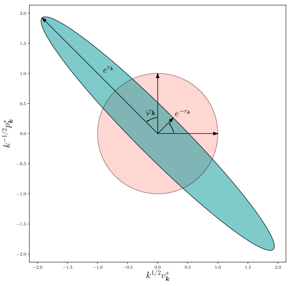
Figure 1: Phase space representation of the $\textstyle\sqrt{2\,}$ -$\sigma$ contour level of the Wigner function $W^{s}$, for $\varphi_{\bm{k}}=\pi/4$, $r_{\bm{k}}=1$ (green ellipse) compared to the pink circle corresponding to a vacuum state (coherent state) with vanishing squeezing.

This implies that the semi-minor and the semi-major axes of the above-mentioned ellipses are tilted by the angle $\varphi_{k}$ in phase space, and that for the $\textstyle\sqrt{2\,}$ -$\sigma$ contour, their respective lengths are given by $e^{r_{k}}$ and $e^{-r_{k}}$. Such an ellipse is displayed in Fig. 1, and fully describes the quantum state of the system. This leads to a simple interpretation of the squeezing parameters: $r_{k}$ controls the eccentricity of the Wigner-function contours, and $\varphi_{k}$ its phase-space orientation.

Note that the area of the ellipse, which is proportional to the product between the semi-major and the semi-minor axes lengths, is a constant. This can be traced back to the fact that it is proportional to the determinant of the covariance matrix, which is a constant given that the time evolution is performed via a symplectic matrix in Eq. (3.6). Alternatively, it can also be seen as a consequence of Eq. (3.3). Since the determinant of the covariance matrix is related to the purity of the state via Eq. (2.26), it also simply translates the fact that the state remains pure if it does not couple to an environment.

3.3 Transport equations

The third method which allows us to follow the time evolution of the system is to establish the differential equations obeyed by the components of the covariance matrix, i.e. by the two-point functions of the system. In general, the quantum expectation value of any operator $\hat{O}$ evolves according to the Heisenberg equation

$$\frac{\mathrm{d}\langle\hat{O}\rangle}{\mathrm{d}{\tau}} =\left\langle\frac{\partial\hat{O}}{\partial{\tau}}\right\rangle-i\left\langle\left[\hat{O},\hat{H}\right]\right\rangle.$$ (3.28)

For one-point correlation functions, using the Hamiltonian (2.7), this leads

$$\frac{\mathrm{d}\langle v_{\bm{k}}^{s}\rangle}{\mathrm{d}{\tau}}=\langle p_{\bm{k}}^{s}\rangle,\quad\frac{\mathrm{d}\langle p_{\bm{k}}^{s}\rangle}{\mathrm{d}{\tau}}=-\omega^{2}(k,\tau)\langle v_{\bm{k}}^{s}\rangle\,,$$ (3.29)

which is nothing but Ehrenfest’s theorem. Combined together, these two equations lead to $\langle\hat{v}_{\bm{k}}^{s}\rangle^{\prime\prime}+\omega^{2}(k,\tau)\langle\hat{v}_{\bm{k}}^{s}\rangle=0$, which coincides with the equation satisfied by the combination $u_{k}+w_{k}^{*}$ of the Bogoliubov coefficients, see Eq. (3.4), and which is nothing but the classical equation of motion.

For two-point correlation functions, one has

$$\frac{\mathrm{d}}{\mathrm{d}{\tau}}\langle\hat{v}_{{\bm{k}}_{1}}^{s}\hat{v}_{{\bm{k}}_{2}}^{s}\rangle =\langle\hat{v}_{{\bm{k}}_{1}}^{s}\hat{p}_{{\bm{k}}_{2}}^{s}+\hat{p}_{{\bm{k}}_{1}}^{s}\hat{v}_{{\bm{k}}_{2}}^{s}\rangle,$$ (3.30)

$$\frac{\mathrm{d}}{\mathrm{d}{\tau}}\langle\hat{p}_{{\bm{k}}_{1}}^{s}\hat{v}_{{\bm{k}}_{2}}^{s}\rangle =\langle\hat{p}_{{\bm{k}}_{1}}^{s}\hat{p}_{{\bm{k}}_{2}}^{s}\rangle-\omega^{2}(k_{1},\tau)\langle\hat{v}_{{\bm{k}}_{1}}^{s}\hat{v}_{{\bm{k}}_{2}}^{s}\rangle,$$ (3.31)

$$\frac{\mathrm{d}}{\mathrm{d}{\tau}}\langle\hat{v}_{{\bm{k}}_{1}}^{s}\hat{p}_{{\bm{k}}_{2}}^{s}\rangle =\langle\hat{p}_{{\bm{k}}_{1}}^{s}\hat{p}_{{\bm{k}}_{2}}^{s}\rangle-\omega^{2}(k_{2},\tau)\langle\hat{v}_{{\bm{k}}_{1}}^{s}\hat{v}_{{\bm{k}}_{2}}^{s}\rangle,$$ (3.32)

$$\frac{\mathrm{d}}{\mathrm{d}{\tau}}\langle\hat{p}_{{\bm{k}}_{1}}^{s}\hat{p}_{{\bm{k}}_{2}}^{s}\rangle =-\omega^{2}(k_{2},\tau)\langle\hat{p}_{{\bm{k}}_{1}}^{s}\hat{v}_{{\bm{k}}_{2}}^{s}\rangle-\omega^{2}(k_{1},\tau)\langle\hat{v}_{{\bm{k}}_{1}}^{s}\hat{p}_{{\bm{k}}_{2}}^{s}\rangle,$$ (3.33)

where, as expected, the time derivative of correlators mixing R and I quantities vanish, i.e. $\mathrm{d}{\langle R^{s}_{i}R^{\tilde{s}}_{j}\rangle}/(\mathrm{d}{\tau})\propto\delta(s-\tilde{s})$. Making use of Eqs. (2.20)-(2.22), this leads to the following differential system for the entries of the covariance matrix,

$$\frac{1}{k}\frac{\mathrm{d}\gamma_{11}}{\mathrm{d}{\tau}} =\gamma_{12}+\gamma_{21},$$ (3.34)

$$\frac{1}{k}\frac{\mathrm{d}}{\mathrm{d}{\tau}}(\gamma_{12}+\gamma_{21}) =2\gamma_{22}-2\frac{\omega^{2}}{k^{2}}\gamma_{11},$$ (3.35)

$$\frac{1}{k}\frac{\mathrm{d}\gamma_{22}}{\mathrm{d}{\tau}} =-\frac{\omega^{2}}{k^{2}}(\gamma_{12}+\gamma_{21}).$$ (3.36)

Let us recall that, as pointed out below Eq. (3.15), if the initial state is chosen to be the vacuum state, these equations must be solved with initial conditions $\gamma_{11}(\tau_{\mathrm{in}})=\gamma_{22}(\tau_{\mathrm{in}})=1$ and $(\gamma_{12}+\gamma_{21})(\tau_{\mathrm{in}})=0$. One can check that, in agreement with the remark made at the end of Sec. 3.2, these equations imply that $\det\gamma^{s}=\gamma_{11}\gamma_{22}-\gamma_{12}\gamma_{21}$ is preserved in time. One may also note that the above three first-order differential equations lead to a single, third-order, differential equation for $\gamma_{11}$, namely

$$\frac{1}{k^{3}}\frac{{\mathrm{d}}^{3}\gamma_{11}}{{\mathrm{d}}{\tau}^{3}} +4\frac{\omega^{2}}{k^{2}}\frac{1}{k}\frac{{\mathrm{d}}\gamma_{11}}{{\mathrm{d}}{\tau}}+\frac{2}{k}\frac{{\mathrm{d}}}{{\mathrm{d}}{\tau}}\left(\frac{\omega^{2}}{k^{2}}\right)\gamma_{11}=0.$$ (3.37)

The order of that differential equation can however be reduced upon introducing the (complex) change of variable $\gamma_{11}=v_{k}v_{k}^{*}$. Indeed, one can show that Eq. (3.37) is satisfied if $v_{k}^{\prime\prime}+\omega^{2}v_{k}=0$. One recovers again the same second-order differential equation as the one satisfied by the combination of Bogoliubov coefficients $u_{k}+w_{k}^{*}$, see Eq. (3.4) [note that the initial conditions also match, i.e. the initial conditions give above for $\gamma_{11}$, $\gamma_{12}$ and $\gamma_{22}$ lead to $v_{k}({\tau}_{\mathrm{in}})=1$ and $v_{k}^{\prime}({\tau}_{\mathrm{in}})=-ik$], which also coincides with the classical equation of motion as pointed out above. This shows that the evolution of Gaussian quantum states can be entirely described by the dynamics of its classical counterpart, and that the three approaches introduced above to solve the dynamics are technically equivalent.

3.4 Quantum discord

As explained in Sec. 2.4, the computation of quantum discord boils down to the computation of the symplectic eigenvalue $\sigma(\theta)$. Setting $\theta=0$ in Eq. (2.27) leads to $\sigma(0)=\mathchoice{{\hbox{$\displaystyle\sqrt{\det\gamma^{s}\,}$}\lower 0.4pt\hbox{\vrule height=6.94444pt,depth=-5.55559pt}}}{{\hbox{$\textstyle\sqrt{\det\gamma^{s}\,}$}\lower 0.4pt\hbox{\vrule height=6.94444pt,depth=-5.55559pt}}}{{\hbox{$\scriptstyle\sqrt{\det\gamma^{s}\,}$}\lower 0.4pt\hbox{\vrule height=4.8611pt,depth=-3.8889pt}}}{{\hbox{$\scriptscriptstyle\sqrt{\det\gamma^{s}\,}$}\lower 0.4pt\hbox{\vrule height=3.47221pt,depth=-2.77779pt}}}$, so for a pure state, one has $\sigma(0)=1$. Since Eq. (2.29) leads to $f(1)=0$, the expression (2.28) for quantum discord reduces to

$$\mathcal{D}=f\left[\sigma(\theta)\right]\,.$$ (3.38)

The symplectic eigenvalue $\sigma(\theta)$ can be expressed in terms of the Bogoliubov coefficients by plugging Eq. (3.14) into Eq. (2.27), and one finds $\sigma(\theta)=\mathchoice{{\hbox{$\displaystyle\sqrt{1+4|u_{k}|^{2}|w_{k}|^{2}\sin^{2}(2\theta)\,}$}\lower 0.4pt\hbox{\vrule height=9.30444pt,depth=-7.44359pt}}}{{\hbox{$\textstyle\sqrt{1+4|u_{k}|^{2}|w_{k}|^{2}\sin^{2}(2\theta)\,}$}\lower 0.4pt\hbox{\vrule height=9.30444pt,depth=-7.44359pt}}}{{\hbox{$\scriptstyle\sqrt{1+4|u_{k}|^{2}|w_{k}|^{2}\sin^{2}(2\theta)\,}$}\lower 0.4pt\hbox{\vrule height=6.53888pt,depth=-5.23112pt}}}{{\hbox{$\scriptscriptstyle\sqrt{1+4|u_{k}|^{2}|w_{k}|^{2}\sin^{2}(2\theta)\,}$}\lower 0.4pt\hbox{\vrule height=5.03888pt,depth=-4.03113pt}}}$. Making use of Eq. (3.16), it can also be written in terms of the squeezing parameters as

$$\sigma(\theta)=\mathchoice{{\hbox{$\displaystyle\sqrt{1+\sinh^{2}(2r_{k})\sin^{2}(2\theta)\,}$}\lower 0.4pt\hbox{\vrule height=8.74889pt,depth=-6.99915pt}}}{{\hbox{$\textstyle\sqrt{1+\sinh^{2}(2r_{k})\sin^{2}(2\theta)\,}$}\lower 0.4pt\hbox{\vrule height=8.74889pt,depth=-6.99915pt}}}{{\hbox{$\scriptstyle\sqrt{1+\sinh^{2}(2r_{k})\sin^{2}(2\theta)\,}$}\lower 0.4pt\hbox{\vrule height=6.14998pt,depth=-4.92001pt}}}{{\hbox{$\scriptscriptstyle\sqrt{1+\sinh^{2}(2r_{k})\sin^{2}(2\theta)\,}$}\lower 0.4pt\hbox{\vrule height=4.7611pt,depth=-3.8089pt}}}\,,$$ (3.39)

where only the squeezing amplitude $r_{k}$ enters the expression. This shows that, when $\theta\neq 0$, the discord increases with the squeezing amplitude but does not depend on the squeezing angle. Let us also mention that, plugging Eq. (2.23) into Eq. (2.27), one obtains an expression that only involves the number of particles $\mathcal{N}_{k}$, namely

$$\sigma(\theta)=\mathchoice{{\hbox{$\displaystyle\sqrt{1+4\sin^{2}(2\theta)\mathcal{N}_{k}\left(\mathcal{N}_{k}+1\right)\,}$}\lower 0.4pt\hbox{\vrule height=8.48303pt,depth=-6.78645pt}}}{{\hbox{$\textstyle\sqrt{1+4\sin^{2}(2\theta)\mathcal{N}_{k}\left(\mathcal{N}_{k}+1\right)\,}$}\lower 0.4pt\hbox{\vrule height=8.48303pt,depth=-6.78645pt}}}{{\hbox{$\scriptstyle\sqrt{1+4\sin^{2}(2\theta)\mathcal{N}_{k}\left(\mathcal{N}_{k}+1\right)\,}$}\lower 0.4pt\hbox{\vrule height=5.96388pt,depth=-4.77113pt}}}{{\hbox{$\scriptscriptstyle\sqrt{1+4\sin^{2}(2\theta)\mathcal{N}_{k}\left(\mathcal{N}_{k}+1\right)\,}$}\lower 0.4pt\hbox{\vrule height=4.62817pt,depth=-3.70256pt}}}\,.$$ (3.40)

This shows that discord increases with the number of entangled particles created between the sectors $\bm{k}$ and $-\bm{k}$, as expected. This also indicates that discord is maximal when $\theta=-\pi/4$, i.e. in the partition $\pm\bm{k}$. These considerations are in agreement with the results found in Ref. [5].

4 Discord in the presence of an environment

In Sec. 3, we have described the evolution of the system and its quantum discord in the case where it is placed in a pure state, without interactions with environmental degrees of freedom. We now study how these considerations generalise to the situation where an environment is present and couples to the system. Formally, we write down the total Hamiltonian as the sum of a term acting on the system, $\hat{H}$, a term acting on the environment, $\hat{H}_{\mathrm{env}}$, and an interaction term, $\hat{H}_{\mathrm{int}}$,

$$\hat{H}_{\mathrm{tot}}=\hat{H}\otimes\hat{\mathbb{I}}_{\mathrm{env}}+\hat{\mathbb{I}}\otimes\hat{H}_{\mathrm{env}}+g\hat{H}_{\mathrm{int}},$$ (4.1)

where $g$ is a coupling constant that controls the interaction strength and we recall that $\hat{H}$ is given in Eq. (2.7). Our goal is to analyse the state of the system, which is described by the reduced density matrix

$$\hat{\rho}=\mathrm{Tr}_{\mathrm{env}}\left(\hat{\rho}_{\mathrm{tot}}\right)\,.$$ (4.2)

In practice, we assume that the interaction term is local, so it can be written as

$$\hat{H}_{\mathrm{int}}(\tau)=\int\mathrm{d}^{3}{\bm{x}}\,\hat{A}(\tau,{\bm{x}})\otimes\hat{E}(\tau,{\bm{x}}),$$ (4.3)

where $\hat{A}$ is an operator acting in the Hilbert space of the system and $\hat{E}$ an operator acting in the Hilbert space of the environment.

4.1 Caldeira-Leggett model

Under the assumption that the auto-correlation time of $\hat{E}$ in the environment, which we denote $\tau_{\mathrm{c}}$, is much shorter than the time scale over which the system evolves, one can show that the reduced density matrix (4.2) obeys the Lindblad equation [31, 32, 15, 33, 34]

$$\frac{\mathrm{d}\hat{\rho}}{\mathrm{d}{\tau}} =-i\left[\hat{H},\hat{\rho}\right]-\frac{\Gamma}{2}\int\mathrm{d}^{3}{\bm{x}}\,\mathrm{d}^{3}{\bm{y}}\,C_{E}(\tau;{\bm{x}},{\bm{y}})\left[\hat{A}({\bm{x}}),\left[\hat{A}({\bm{y}}),\hat{\rho}\right]\right],$$ (4.4)

where $C_{E}({\tau};{\bm{x}},{\bm{y}})=\langle\hat{E}({\tau},{\bm{x}})\hat{E}({\tau},{\bm{y}})\rangle$ is the equal-time correlation function of $\hat{E}$, and $\Gamma\equiv 2g^{2}\tau_{\mathrm{c}}$. Let us note that the Lindblad equation generates all quantum dynamical semigroups [35], and that even though it is derived at leading order in $g$, it allows for efficient late-time re-summation [36].

Similarly to Eq. (3.28), the equation controlling the quantum expectation value of a given operator $\hat{O}$, namely $\langle\hat{O}\rangle=\mathrm{Tr}(\hat{\rho}\,\hat{O})$, can be obtained from the Lindblad equation, and one finds

$$\frac{\mathrm{d}\langle\hat{O}\rangle}{\mathrm{d}{\tau}} =\left\langle\frac{\partial\hat{O}}{\partial{\tau}}\right\rangle-i\left\langle\left[\hat{O},\hat{H}\right]\right\rangle -\frac{\Gamma}{2}(2\pi)^{3/2}\int_{\mathbb{R}^{3}}\mathrm{d}^{3}{\bm{k}}\,\tilde{C}_{E}({\tau},{\bm{k}})\left\langle\left[\left[\hat{O},\hat{A}_{\bm{k}}\right],\hat{A}_{-{\bm{k}}}\right]\right\rangle,$$ (4.5)

where $\tilde{C}_{E}({\tau},{\bm{k}})$ is the Fourier transform of the correlation function [assuming statistical homogeneity, $C_{{E}}(\bm{x},\bm{y})$ depends only on $\bm{x}-\bm{y}$, so we mean the Fourier transform with respect to $\bm{x}-\bm{y}$].

These equations are difficult to solve in general, but they greatly simplify under the assumption that $\hat{A}$ is linear in the phase-space variables. The reason is that, in that case, all interactions involving the system are linear, so the state of the system remains Gaussian (although it becomes a mixed state). This allows one to still fully describe it in terms of a covariance matrix, and to generalise most of the considerations presented in Sec. 3. Such a setup is called the Caldeira-Leggett model [37, 38, 39], and in what follows we will use it to understand how decoherence may affect the presence of quantum discord within the system. For simplicity, we will consider the case where $\hat{A}=\hat{v}$, but the more generic situation where $\hat{A}$ is a linear combination of $\hat{v}$ and $\hat{p}$ can be dealt with along very similar lines, see Ref. [19].

4.2 Transport equations

Let us first follow the approach presented in Sec. 3.3 and derive transport equations from Eq. (4.5). For one-point correlation functions, one still obtains Eq. (3.29), i.e. the classical equations of motion. For two-point correlation functions, one finds

$$\frac{\mathrm{d}}{\mathrm{d}{\tau}}\langle\hat{v}_{{\bm{k}}_{1}}^{s}\hat{v}_{{\bm{k}}_{2}}^{s}\rangle =\langle\hat{v}_{{\bm{k}}_{1}}^{s}\hat{p}_{{\bm{k}}_{2}}^{s}+\hat{p}_{{\bm{k}}_{1}}^{s}\hat{v}_{{\bm{k}}_{2}}^{s}\rangle,$$ (4.6)

$$\frac{\mathrm{d}}{\mathrm{d}{\tau}}\langle\hat{p}_{{\bm{k}}_{1}}^{s}\hat{v}_{{\bm{k}}_{2}}^{s}\rangle =\langle\hat{p}_{{\bm{k}}_{1}}^{s}\hat{p}_{{\bm{k}}_{2}}^{s}\rangle-\omega^{2}({k}_{1},\tau)\langle\hat{v}_{{\bm{k}}_{1}}^{s}\hat{v}_{{\bm{k}}_{2}}^{s}\rangle,$$ (4.7)

$$\frac{\mathrm{d}}{\mathrm{d}{\tau}}\langle\hat{v}_{{\bm{k}}_{1}}^{s}\hat{p}_{{\bm{k}}_{2}}^{s}\rangle =\langle\hat{p}_{{\bm{k}}_{1}}^{s}\hat{p}_{{\bm{k}}_{2}}^{s}\rangle-\omega^{2}({k}_{2},\tau)\langle\hat{v}_{{\bm{k}}_{1}}^{s}\hat{v}_{{\bm{k}}_{2}}^{s}\rangle,$$ (4.8)

$$\frac{\mathrm{d}}{\mathrm{d}{\tau}}\langle\hat{p}_{{\bm{k}}_{1}}^{s}\hat{p}_{{\bm{k}}_{2}}^{s}\rangle =-\omega^{2}({k}_{2},\tau)\langle\hat{p}_{{\bm{k}}_{1}}^{s}\hat{v}_{{\bm{k}}_{2}}^{s}\rangle-\omega^{2}({k}_{1},\tau)\langle\hat{v}_{{\bm{k}}_{1}}^{s}\hat{p}_{{\bm{k}}_{2}}^{s}\rangle+\Gamma(2\pi)^{3/2}\tilde{C}_{E}(\tau,{\bm{k}}_{1})\delta({\bm{k}}_{2}-{\bm{k}}_{1}),$$ (4.9)

where correlators mixing R and I quantities still vanish, i.e. ${\langle R^{s}_{i}R^{\tilde{s}}_{j}\rangle}\propto\delta(s-\tilde{s})$. Compared to Eqs. (3.30)-(3.33), one can see that only the last equation gets modified, and receives an additional contribution proportional to $\Gamma$. Making use of Eqs. (2.20)-(2.22), this leads to the following differential system for the entries of the covariance matrix,

$$\frac{1}{k}\frac{\mathrm{d}\gamma_{11}}{\mathrm{d}{\tau}} =\gamma_{12}+\gamma_{21},$$ (4.10)

$$\frac{1}{k}\frac{\mathrm{d}}{\mathrm{d}{\tau}}(\gamma_{12}+\gamma_{21}) =2\gamma_{22}-2\frac{\omega^{2}}{k^{2}}\gamma_{11},$$ (4.11)

$$\frac{1}{k}\frac{\mathrm{d}\gamma_{22}}{\mathrm{d}{\tau}} =-\frac{\omega^{2}}{k^{2}}(\gamma_{12}+\gamma_{21})+2\Gamma(2\pi)^{3/2}\frac{\tilde{C}_{E}}{k^{2}}\,,$$ (4.12)

which should be compared with Eqs. (3.34)-(3.36). Let us recall that, under the assumption that the system is initially in the vacuum state, these equations should be solved with initial conditions $\gamma_{11}({\tau}_{\mathrm{in}})=1$, $(\gamma_{12}+\gamma_{21})({\tau}_{\mathrm{in}})=0$ and $\gamma_{22}({\tau}_{\mathrm{in}})=1$.

Another important consequence of these transport equations is that they lead to the following evolution for $\det(\gamma^{s})=\gamma_{11}\gamma_{22}-\gamma_{12}^{2}$:

$$\frac{\mathrm{d}}{\mathrm{d}{\tau}}\det\left(\gamma^{s}\right)=2\Gamma\gamma_{11}(2\pi)^{3/2}\frac{\tilde{C}_{{E}}}{k}.$$ (4.13)

When $\Gamma=0$, i.e. in the absence of an environment, one recovers the fact that this determinant is preserved, hence the system remains in a pure state. Otherwise, Eq. (4.13) indicates that the interaction with the environment induces decoherence of the system, since it makes the purity decrease away from one, see Eq. (2.26).

Finally, similarly to Eq. (3.37), one can derive a single, third-order differential equation for $\gamma_{11}$, which reads

$$\frac{1}{k^{3}}\frac{{\mathrm{d}}^{3}\gamma_{11}}{{\mathrm{d}}{\tau}^{3}} +4\frac{\omega^{2}}{k^{2}}\frac{1}{k}\frac{{\mathrm{d}}\gamma_{11}}{{\mathrm{d}}{\tau}}+\frac{2}{k}\frac{{\mathrm{d}}}{{\mathrm{d}}\tau}\left(\frac{\omega^{2}}{k^{2}}\right)\gamma_{11}=4\Gamma(2\pi)^{3/2}\frac{\tilde{C}_{E}}{k^{2}}\,.$$ (4.14)

As pointed out below Eq. (3.37), in the absence of a source term in the right-hand side, the solution to this equation reads $\gamma_{11}=v_{k}v_{k}^{*}$, where $v_{k}$ satisfies the classical equation of motion $v_{k}^{\prime\prime}+\omega^{2}v_{k}=0$. Using Green’s function method, the solution in the presence of a source term is thus given by

$$\gamma_{11}(\tau)=v_{k}(\tau)v_{k}^{*}(\tau)-\frac{8k}{W^{2}}(2\pi)^{3/2}\int_{\tau_{\mathrm{in}}}^{\tau}\Gamma({\tau}^{\prime})\,\tilde{C}_{E}({\tau}^{\prime},k)\,\Im\mathrm{m}\,^{2}\left[v_{k}(\tau)v_{k}^{*}({\tau}^{\prime})\right]{\mathrm{d}}{\tau}^{\prime},$$ (4.15)

where $W\equiv v_{k}v_{k}^{*}{}^{\prime}-v_{k}^{*}v_{k}^{\prime}$ is the Wronksian of the $v_{k}$ mode function. Given the equation of motion that $v_{k}$ satisfies, one can readily show that $W$ is preserved in time. It can therefore be evaluated at initial time, where the initial conditions derived for $v_{k}$ below Eq. (3.37) lead to $W=2ik$. Using Eqs. (4.10) and (4.11) again, one thus obtains the following expressions for the entries of the covariance matrix,

$$\gamma_{11} =\left|v_{k}\right|^{2}+\mathcal{I}_{k},\qquad\gamma_{12}=\frac{\Re\mathrm{e}\,\left(v_{k}v^{*\,\prime}_{k}\right)}{k}+\mathcal{J}_{k},\qquad\gamma_{22}=\frac{\left|v_{k}^{\prime}\right|^{2}}{k^{2}}+\mathcal{K}_{k}\,,$$ (4.16)

where

$$\mathcal{I}_{k}(\tau) =\frac{2}{k}(2\pi)^{3/2}\int_{{\tau}_{\mathrm{in}}}^{\tau}\Gamma({\tau}^{\prime})\,\tilde{C}_{E}({\tau}^{\prime},k)\,\Im\mathrm{m}\,^{2}\left[v_{k}({\tau}^{\prime})v_{k}^{*}(\tau)\right]{\mathrm{d}}{\tau}^{\prime}\,,$$ (4.17)

$$\mathcal{J}_{k}(\tau) =\frac{2}{k^{2}}(2\pi)^{3/2}\int_{{\tau}_{\mathrm{in}}}^{\tau}\Gamma({\tau}^{\prime})\,\tilde{C}_{E}({\tau}^{\prime},k)\,\Im\mathrm{m}\,\left[v_{k}({\tau}^{\prime})v_{k}^{*}(\tau)\right]\Im\mathrm{m}\,\left[v_{k}({\tau}^{\prime})v_{k}^{*\prime}(\tau)\right]{\mathrm{d}}{\tau}^{\prime}\,,$$ (4.18)

$$\mathcal{K}_{k}(\tau) =\frac{2}{k^{3}}(2\pi)^{3/2}\int_{{\tau}_{\mathrm{in}}}^{\tau}\Gamma({\tau}^{\prime})\,\tilde{C}_{E}({\tau}^{\prime},k)\Im\mathrm{m}\,^{2}\left[v_{k}({\tau}^{\prime})v_{k}^{*\prime}(\tau)\right]\mathrm{d}{\tau}^{\prime}\,.$$ (4.19)

These formula provide an explicit expression for the covariance matrix, hence for the full quantum state of the reduced system.

4.3 Generalised squeezing parameters

We now follow the approach presented in Sec. 3.2 where the quantum state of the system is described in terms of squeezing parameters. Note that the Bogoliubov coefficients introduced in Sec. 3.1 cannot be directly generalised to the case where an environment is present, since they are related to the unitary evolution of the system. Therefore, one cannot use Eq. (3.16) to define squeezing parameters in the present situation. However, the geometrical interpretation developed around Fig. 1 can still be used to introduce generalised squeezing parameters. This will be particularly useful to understand the state purity, and quantum discord, from a phase-space geometrical perspective.

In the Caldeira-Leggett model indeed, the state is still described by a covariance matrix, that can still be diagonalised as in Eq. (3.27). The only difference is that, as mentioned around Eq. (4.13), the determinant of the covariance matrix does not remain equal to one. This introduces a new “squeezing parameter”, denoted $\lambda_{k}\equiv\det(\gamma^{s})$, such that Eq. (3.27) becomes

$$(\widetilde{\gamma}^{s})^{-1}=\lambda_{k}^{-1/2}\begin{pmatrix}e^{2r_{k}}&0\\ 0&e^{-2r_{k}}\end{pmatrix}.$$ (4.20)

Performing the phase-space rotation of angle $\varphi_{k}$ introduced in Eq. (3.27), this leads to the following expression for the covariance matrix in the $\mathrm{R}/\mathrm{I}$ partition,

$$\gamma^{s}=\mathchoice{{\hbox{$\displaystyle\sqrt{\lambda_{k}\,}$}\lower 0.4pt\hbox{\vrule height=6.94444pt,depth=-5.55559pt}}}{{\hbox{$\textstyle\sqrt{\lambda_{k}\,}$}\lower 0.4pt\hbox{\vrule height=6.94444pt,depth=-5.55559pt}}}{{\hbox{$\scriptstyle\sqrt{\lambda_{k}\,}$}\lower 0.4pt\hbox{\vrule height=4.8611pt,depth=-3.8889pt}}}{{\hbox{$\scriptscriptstyle\sqrt{\lambda_{k}\,}$}\lower 0.4pt\hbox{\vrule height=3.47221pt,depth=-2.77779pt}}}\begin{pmatrix}\cosh\left(2r_{k}\right)-\cos\left(2\varphi_{k}\right)\sinh\left(2r_{k}\right)&-\sin\left(2\varphi_{k}\right)\sinh\left(2r_{k}\right)\\ -\sin\left(2\varphi_{k}\right)\sinh\left(2r_{k}\right)&\cosh\left(2r_{k}\right)+\cos\left(2\varphi_{k}\right)\sinh\left(2r_{k}\right)\end{pmatrix}\,,$$ (4.21)

which generalises Eqs. (3.20)-(3.22). This shows that, in the Caldeira-Leggett model, the quantum state of the system can still be described with an ellipse in phase space, where $r_{k}$ describes the eccentricity of the ellipse, $\varphi_{k}$ its orientation, and $\lambda_{k}$ its area (which is given by $\pi\lambda_{k}$).

Note that equations of motion for the generalised squeezing parameters $r_{k}$, $\varphi_{k}$ and $\lambda_{k}$ can also be derived, by plugging Eq. (4.21) into Eqs. (4.10)-(4.12). This leads to

$$\frac{{\mathrm{d}}\lambda_{k}}{{\mathrm{d}}{\tau}} =2\Gamma(2\pi)^{3/2}\frac{\tilde{C}_{E}}{k}\lambda_{k}^{1/2}\left[\cosh\left(2r_{k}\right)-\cos\left(2\varphi_{k}\right)\sinh\left(2r_{k}\right)\right],$$ (4.22)

$$\frac{{\mathrm{d}}r_{k}}{{\mathrm{d}}{\tau}} =\frac{k}{2}\left(\frac{\omega^{2}}{k^{2}}-1\right)\sin(2\varphi_{k})-\frac{\Gamma}{\mathchoice{{\hbox{$\displaystyle\sqrt{\lambda_{k}\,}$}\lower 0.4pt\hbox{\vrule height=6.94444pt,depth=-5.55559pt}}}{{\hbox{$\textstyle\sqrt{\lambda_{k}\,}$}\lower 0.4pt\hbox{\vrule height=6.94444pt,depth=-5.55559pt}}}{{\hbox{$\scriptstyle\sqrt{\lambda_{k}\,}$}\lower 0.4pt\hbox{\vrule height=4.8611pt,depth=-3.8889pt}}}{{\hbox{$\scriptscriptstyle\sqrt{\lambda_{k}\,}$}\lower 0.4pt\hbox{\vrule height=3.47221pt,depth=-2.77779pt}}}}\frac{(2\pi)^{3/2}}{2}\frac{\tilde{C}_{E}}{k}\left[\sinh\left(2r_{k}\right)-\cos\left(2\varphi_{k}\right)\cosh\left(2r_{k}\right)\right],$$ (4.23)

$$\frac{{\mathrm{d}}\varphi_{k}}{{\mathrm{d}}{\tau}} =-\frac{k}{2}\left(\frac{\omega^{2}}{k^{2}}+1\right)+\frac{k}{2}\left(\frac{\omega^{2}}{k^{2}}-1\right)\frac{\cos(2\varphi_{k})}{\tanh(2r_{k})}-\Gamma\frac{\sin(2\varphi_{k})}{2\sinh(2r_{k})\mathchoice{{\hbox{$\displaystyle\sqrt{\lambda_{k}\,}$}\lower 0.4pt\hbox{\vrule height=6.94444pt,depth=-5.55559pt}}}{{\hbox{$\textstyle\sqrt{\lambda_{k}\,}$}\lower 0.4pt\hbox{\vrule height=6.94444pt,depth=-5.55559pt}}}{{\hbox{$\scriptstyle\sqrt{\lambda_{k}\,}$}\lower 0.4pt\hbox{\vrule height=4.8611pt,depth=-3.8889pt}}}{{\hbox{$\scriptscriptstyle\sqrt{\lambda_{k}\,}$}\lower 0.4pt\hbox{\vrule height=3.47221pt,depth=-2.77779pt}}}}(2\pi)^{3/2}\frac{\tilde{C}_{E}}{k}.$$ (4.24)

One can check that, in the limit $\Gamma\to 0$, Eqs. (3.17) are recovered, and that Eq. (4.22) is essentially a rewriting of Eq. (4.13) for the non-conservation of the determinant.

4.4 Quantum discord

Let us now turn to the main goal of this article, namely the calculation of the quantum discord in the presence of an environment. As explained in Sec. 2.4, a single quantity needs to be computed, namely $\sigma(\theta)$ given in Eq. (2.27), which in terms of the generalised squeezing parameters reads

$$\sigma(\theta)=\lambda_{k}^{1/2}\mathchoice{{\hbox{$\displaystyle\sqrt{1+\sinh^{2}(2r_{k})\sin^{2}(2\theta)\,}$}\lower 0.4pt\hbox{\vrule height=8.74889pt,depth=-6.99915pt}}}{{\hbox{$\textstyle\sqrt{1+\sinh^{2}(2r_{k})\sin^{2}(2\theta)\,}$}\lower 0.4pt\hbox{\vrule height=8.74889pt,depth=-6.99915pt}}}{{\hbox{$\scriptstyle\sqrt{1+\sinh^{2}(2r_{k})\sin^{2}(2\theta)\,}$}\lower 0.4pt\hbox{\vrule height=6.14998pt,depth=-4.92001pt}}}{{\hbox{$\scriptscriptstyle\sqrt{1+\sinh^{2}(2r_{k})\sin^{2}(2\theta)\,}$}\lower 0.4pt\hbox{\vrule height=4.7611pt,depth=-3.8089pt}}}\,.$$ (4.25)

Plugging this expression into Eq. (2.28), one obtains an explicit formula for quantum discord in terms of three parameters only: the squeezing amplitude $r_{k}$, the state purity $\mathrm{Tr}(\hat{\rho}^{2})=1/\lambda_{k}$, and the partition angle $\theta$. This formula is displayed in Fig. 2 for $\theta=-\pi/4$ (left panel, corresponding to the $\pm\bm{k}$ partition) and $\theta=0.1$ (right panel).

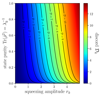
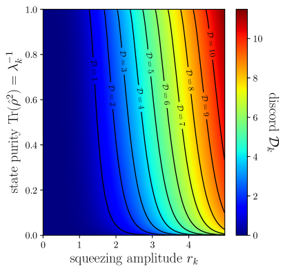
Figure 2: Quantum discord $\mathcal{D}_{k}$ in terms of the generalised squeezing amplitude $r_{k}$ and the state purity $\mathrm{Tr}(\hat{\rho}^{2})=1/\lambda_{k}$, for $\theta=-\pi/4$ (left panel) and $\theta=0.1$ (right panel). The black solid lines show a few contour lines of $\mathcal{D}_{k}$.

One can see that, as the squeezing amplitude increases, quantum discord increases, as in the case where no environment was present. When the state purity decreases, quantum discord decreases, which means that interactions with an environment tend to reduce the amount of quantum correlations. This is in agreement with the common lore that decoherence is associated with the emergence of classical properties. One can also check that quantum discord increases with the partition angle as it varies between $0$ and $\pi/4$, i.e. as it interpolates between the $\mathrm{R}/\mathrm{I}$ partition which is separable (hence uncorrelated) and the $\pm\bm{k}$ partition where it is maximally correlated and discordant.

In order to gain more analytical insight in the behaviour of quantum discord, let us consider the large-squeezing limit $r_{k}\gg 1$ (this limit is particularly relevant to the cosmological setting considered in Sec. 5). From Eq. (2.28), it is clear that different behaviours are obtained depending on whether $\sigma(\theta)/\sigma^{2}(0)$ is small or large. In the large-squeezing limit, this ratio is given by

$$\frac{\sigma(\theta)}{\sigma^{2}(0)}\simeq\lambda_{k}^{-1/2}e^{2r_{k}}\frac{\left|\sin(2\theta)\right|}{2}\,.$$ (4.26)

In general, as the time evolution proceeds, $r_{k}$ increases (denoting particle creation) and $\lambda_{k}$ increases too (as an effect of decoherence). The two effects therefore compete in Eq. (4.26), and whether the ratio $\sigma(\theta)/\sigma^{2}(0)$ is small or large depends on the details of the dynamics. Expanding Eq. (2.28) in these two limits, one obtains

$$\mathcal{D}_{k}\simeq\begin{cases}\dfrac{2r_{k}}{\ln 2}\quad\text{if}\quad e^{2r_{k}}\left|\sin(2\theta)\right|\gg\mathchoice{{\hbox{$\displaystyle\sqrt{\lambda_{k}\,}$}\lower 0.4pt\hbox{\vrule height=6.94444pt,depth=-5.55559pt}}}{{\hbox{$\textstyle\sqrt{\lambda_{k}\,}$}\lower 0.4pt\hbox{\vrule height=6.94444pt,depth=-5.55559pt}}}{{\hbox{$\scriptstyle\sqrt{\lambda_{k}\,}$}\lower 0.4pt\hbox{\vrule height=4.8611pt,depth=-3.8889pt}}}{{\hbox{$\scriptscriptstyle\sqrt{\lambda_{k}\,}$}\lower 0.4pt\hbox{\vrule height=3.47221pt,depth=-2.77779pt}}}\\ \lambda_{k}^{-1/2}e^{2r_{k}}\dfrac{\left|\sin(2\theta)\right|}{2\ln 2}\quad\text{if}\quad e^{2r_{k}}\left|\sin(2\theta)\right|\ll\mathchoice{{\hbox{$\displaystyle\sqrt{\lambda_{k}\,}$}\lower 0.4pt\hbox{\vrule height=6.94444pt,depth=-5.55559pt}}}{{\hbox{$\textstyle\sqrt{\lambda_{k}\,}$}\lower 0.4pt\hbox{\vrule height=6.94444pt,depth=-5.55559pt}}}{{\hbox{$\scriptstyle\sqrt{\lambda_{k}\,}$}\lower 0.4pt\hbox{\vrule height=4.8611pt,depth=-3.8889pt}}}{{\hbox{$\scriptscriptstyle\sqrt{\lambda_{k}\,}$}\lower 0.4pt\hbox{\vrule height=3.47221pt,depth=-2.77779pt}}}\end{cases}\,.$$ (4.27)

This shows that quantum discord is large in the first case and small in the second case. As a consequence, whether quantum discord is large or small depends on which of squeezing or decoherence wins in the ratio (4.26). This provides a simple criterion for assessing when decoherence substantially reduces the amount of quantum correlations, namely it happens when

$$\mathrm{Tr}(\hat{\rho}^{2})\ll e^{-4r_{k}}\,.$$ (4.28)

A useful geometrical interpretation of Eq. (4.26) is that, according to Eq. (4.20), the combination $\mathchoice{{\hbox{$\displaystyle\sqrt{\lambda_{k}\,}$}\lower 0.4pt\hbox{\vrule height=6.94444pt,depth=-5.55559pt}}}{{\hbox{$\textstyle\sqrt{\lambda_{k}\,}$}\lower 0.4pt\hbox{\vrule height=6.94444pt,depth=-5.55559pt}}}{{\hbox{$\scriptstyle\sqrt{\lambda_{k}\,}$}\lower 0.4pt\hbox{\vrule height=4.8611pt,depth=-3.8889pt}}}{{\hbox{$\scriptscriptstyle\sqrt{\lambda_{k}\,}$}\lower 0.4pt\hbox{\vrule height=3.47221pt,depth=-2.77779pt}}}e^{-2r}$ happens to be the length of the semi-minor axis of the phase-space ellipse. The semi-minor axis increases as an effect of decoherence, which increases the overall area of the ellipse, and decreases because of quantum squeezing: this competition determines whether the semi-minor axis increases or decreases, hence it determines the fate of quantum discord.

Finally, in the same way as we have introduced generalised squeezing parameters, one can extend the definition of the number of particles $\mathcal{N}_{k}$ and the correlation $\mathcal{C}_{k}$, by plugging Eq. (4.21) into Eqs. (2.23)-(2.25), leading to

$$2{\cal N}_{k}+1=\mathchoice{{\hbox{$\displaystyle\sqrt{\lambda_{k}\,}$}\lower 0.4pt\hbox{\vrule height=6.94444pt,depth=-5.55559pt}}}{{\hbox{$\textstyle\sqrt{\lambda_{k}\,}$}\lower 0.4pt\hbox{\vrule height=6.94444pt,depth=-5.55559pt}}}{{\hbox{$\scriptstyle\sqrt{\lambda_{k}\,}$}\lower 0.4pt\hbox{\vrule height=4.8611pt,depth=-3.8889pt}}}{{\hbox{$\scriptscriptstyle\sqrt{\lambda_{k}\,}$}\lower 0.4pt\hbox{\vrule height=3.47221pt,depth=-2.77779pt}}}\cosh\left(2r_{k}\right)\,,\quad 2{\cal C}_{k}=-\mathchoice{{\hbox{$\displaystyle\sqrt{\lambda_{k}\,}$}\lower 0.4pt\hbox{\vrule height=6.94444pt,depth=-5.55559pt}}}{{\hbox{$\textstyle\sqrt{\lambda_{k}\,}$}\lower 0.4pt\hbox{\vrule height=6.94444pt,depth=-5.55559pt}}}{{\hbox{$\scriptstyle\sqrt{\lambda_{k}\,}$}\lower 0.4pt\hbox{\vrule height=4.8611pt,depth=-3.8889pt}}}{{\hbox{$\scriptscriptstyle\sqrt{\lambda_{k}\,}$}\lower 0.4pt\hbox{\vrule height=3.47221pt,depth=-2.77779pt}}}e^{i2\varphi_{k}}\sinh\left(2r_{k}\right)\,.$$ (4.29)

In terms of these parameters, one has $\sigma(\theta)=\mathchoice{{\hbox{$\displaystyle\sqrt{4(\mathcal{N}_{k}+1/2)^{2}-4|\mathcal{C}_{k}|^{2}\cos^{2}(2\theta)\,}$}\lower 0.4pt\hbox{\vrule height=9.30444pt,depth=-7.44359pt}}}{{\hbox{$\textstyle\sqrt{4(\mathcal{N}_{k}+1/2)^{2}-4|\mathcal{C}_{k}|^{2}\cos^{2}(2\theta)\,}$}\lower 0.4pt\hbox{\vrule height=9.30444pt,depth=-7.44359pt}}}{{\hbox{$\scriptstyle\sqrt{4(\mathcal{N}_{k}+1/2)^{2}-4|\mathcal{C}_{k}|^{2}\cos^{2}(2\theta)\,}$}\lower 0.4pt\hbox{\vrule height=6.53888pt,depth=-5.23112pt}}}{{\hbox{$\scriptscriptstyle\sqrt{4(\mathcal{N}_{k}+1/2)^{2}-4|\mathcal{C}_{k}|^{2}\cos^{2}(2\theta)\,}$}\lower 0.4pt\hbox{\vrule height=5.03888pt,depth=-4.03113pt}}}$, which allows one to express quantum discord as a function of $\mathcal{N}_{k}$ and $|\mathcal{C}_{k}|$ only.

5 Application : Cosmological perturbations

In this section, we apply the formalism developed so far to the case of cosmological perturbations. The goal is twofold. First, this will allow us to exemplify in a concrete situation how the tools introduced above work in practice. Second, as explained in Sec. 1, the presence of quantum correlations in the primordial field of cosmological perturbations, and how decoherence might partly remove them, is of great importance regarding our understanding of the origin of cosmic structures as emerging from a quantum-mechanical mechanism, and for our ability to test this aspect of the cosmological scenario.

When the universe is dominated by a single scalar-field, there is a single scalar gauge-invariant perturbation known as the Mukhanov-Sasaki variable [2, 40]. If time is parameterised by conformal time $\eta$, which is related to cosmic time $t$ by $\mathrm{d}{t}=a\mathrm{d}\eta$, where $a$ is the Friedman-Lemaître-Robertson-Walker scale factor, then the Hamiltonian for the Mukhanov-Sasaki variable $v$ is by Eq. (2.7) where

$$\omega^{2}\left(k,\eta\right)=k^{2}-\frac{\left(a\mathchoice{{\hbox{$\displaystyle\sqrt{\epsilon_{1}\,}$}\lower 0.4pt\hbox{\vrule height=4.30554pt,depth=-3.44446pt}}}{{\hbox{$\textstyle\sqrt{\epsilon_{1}\,}$}\lower 0.4pt\hbox{\vrule height=4.30554pt,depth=-3.44446pt}}}{{\hbox{$\scriptstyle\sqrt{\epsilon_{1}\,}$}\lower 0.4pt\hbox{\vrule height=3.01389pt,depth=-2.41113pt}}}{{\hbox{$\scriptscriptstyle\sqrt{\epsilon_{1}\,}$}\lower 0.4pt\hbox{\vrule height=2.15277pt,depth=-1.72223pt}}}\right)^{\prime\prime}}{a\mathchoice{{\hbox{$\displaystyle\sqrt{\epsilon_{1}\,}$}\lower 0.4pt\hbox{\vrule height=4.30554pt,depth=-3.44446pt}}}{{\hbox{$\textstyle\sqrt{\epsilon_{1}\,}$}\lower 0.4pt\hbox{\vrule height=4.30554pt,depth=-3.44446pt}}}{{\hbox{$\scriptstyle\sqrt{\epsilon_{1}\,}$}\lower 0.4pt\hbox{\vrule height=3.01389pt,depth=-2.41113pt}}}{{\hbox{$\scriptscriptstyle\sqrt{\epsilon_{1}\,}$}\lower 0.4pt\hbox{\vrule height=2.15277pt,depth=-1.72223pt}}}}\,.$$ (5.1)

In this expression, a prime denotes derivation with respect to $\eta$, $\epsilon_{1}=1-{\cal H}^{\prime}/{\cal H}^{2}$ is the first slow-roll parameter and ${\cal H}=a^{\prime}/a$.

In practice, we will consider the case of a de-Sitter expansion where $a(\eta)=-1/(H\eta)$ with $H$ the Hubble parameter, since cosmological observations indicate that it is a good proxy for the dynamics of the universe expansion during the inflationary phase. In that case, $\omega^{2}=k^{2}-2/\eta^{2}$, where $\eta$ varies between $-\infty$ to $0$.

5.1 Inflationary perturbations in the absence of an environment

Following the approach presented in Sec. 3.1, let us first derive the Bogoliubov coefficients. The solution of the equation of motion (3.4) satisfied by $v_{k}=u_{k}+w_{k}^{*}$, i.e. $v_{k}^{\prime\prime}+\omega^{2}v_{k}=0$, is given by

$$v_{k}\left(\eta\right)=\left(1-\frac{i}{k\eta}\right)e^{-ik\eta}\,,$$ (5.2)

where we have made use of the initial conditions derived for $v_{k}$ below Eq. (3.37), namely $v_{k}(\eta_{\mathrm{in}})=1$ and $v_{k}^{\prime}(\eta_{\mathrm{in}})=-ik$, at initial time $\eta_{\mathrm{in}}$ set to the infinite past, $\eta_{\mathrm{in}}=-\infty$. As explained below Eq. (3.5), this allows one to derive both Bogoliubov coefficients, and one finds

$$u_{k}=\left(1-\frac{i}{k\eta}-\frac{1}{2k^{2}\eta^{2}}\right)e^{-ik\eta}\,,\qquad\qquad w_{k}^{*}=\frac{1}{2k^{2}\eta^{2}}e^{-ik\eta}\,.$$ (5.3)

One can easily check that these solutions satisfy Eq. (3.3), i.e. $|u_{k}|^{2}-|w_{k}|^{2}=1$. Using Eq. (3.14), one can then calculate the covariance-matrix element and one obtains

$$\gamma_{11}(\eta) =1+\frac{1}{k^{2}\eta^{2}},\qquad\gamma_{12}(\eta)=-\frac{1}{k^{3}\eta^{3}},\qquad\gamma_{22}(\eta)=1-\frac{1}{k^{2}\eta^{2}}+\frac{1}{k^{4}\eta^{4}}.$$ (5.4)

As a consistency check, one can verify that these expressions are solutions of the differential system (3.34)-(3.36), and that they satisfy the initial conditions that were given for it. Finally, the squeezing parameters can be derived from Eqs. (3.20)-(3.22), which lead to

$$\cosh^{2}\left(r_{k}\right) =1+\frac{1}{4(k\eta)^{4}},\quad\tan\left(2\varphi_{k}\right)=\frac{2k\eta}{1-2k^{2}\eta^{2}}.$$ (5.5)

These expressions can be inverted, and one finds

$$r_{k}(\eta) =\frac{1}{2}\mathrm{arccosh}\left[1+\frac{1}{2(k\eta)^{4}}\right]\,,$$ (5.6)

$$\varphi_{k} =\frac{1}{2}\arctan\left(\frac{2k\eta}{1-2k^{2}\eta^{2}}\right)-\frac{\pi}{2}{\mathrm{H}}\left(-k\eta-\frac{1}{\mathchoice{{\hbox{$\displaystyle\sqrt{2\,}$}\lower 0.4pt\hbox{\vrule height=6.44444pt,depth=-5.15558pt}}}{{\hbox{$\textstyle\sqrt{2\,}$}\lower 0.4pt\hbox{\vrule height=6.44444pt,depth=-5.15558pt}}}{{\hbox{$\scriptstyle\sqrt{2\,}$}\lower 0.4pt\hbox{\vrule height=4.51111pt,depth=-3.6089pt}}}{{\hbox{$\scriptscriptstyle\sqrt{2\,}$}\lower 0.4pt\hbox{\vrule height=3.22221pt,depth=-2.57779pt}}}}\right)+\ell\pi\,,$$ (5.7)

where $\ell$ is an integer number and $\mathrm{H}$ is the Heaviside step function defined as $\mathrm{H}(x)=1$ when $x>0$ and $0$ otherwise. One can see that the squeezing amplitude increases as inflation proceeds, and at late time (i.e. when the wavelength of the mode under consideration is much larger than the Hubble radius, $k\ll\mathcal{H}=-1/\eta$), $r_{k}\simeq-2\ln(-k\eta)=2\ln[a/a(k)]$. In this expression, $a(k)$ denotes the value of the scale factor when $k$ crosses out the Hubble scale, i.e. when $k\eta=-1$. For the modes observed in the cosmic microwave background, $\ln[a/a(k)]\simeq 50$ at the end of inflation, hence the squeezing amplitude is of order $100$. The squeezing angle starts out from $\varphi_{k}=-\pi/2$ in the asymptotic past and approaches $0$ at late time, where $\varphi_{k}\simeq k\eta\simeq-a(k)/a\simeq-e^{-r_{k}/2}$ [here we set $\ell=0$ in Eq. (5.7)].

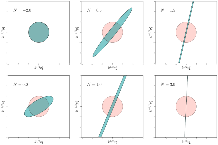
Figure 3: Phase-space ellipse in the plane $(k^{1/2}v_{\bm{k}}^{s},k^{-1/2}p_{\bm{k}}^{s})$ (see the discussion around Fig. 1) at different instants during inflation, labelled by $N=\ln[a/a(k)]$, i.e. the number of $e$-folds measured from the Hubble-crossing time of the mode under consideration. On sub-Hubble scales, the ellipse remains a circle, while it gets squeezed and rotates in the super-Hubble regime.

The evolution of the squeezing parameters is displayed at the level of the phase-space ellipse in Fig. 3. While the mode under consideration remains in the vacuum state, i.e. on sub-Hubble scales when $a\ll a(k)$, the squeezing amplitude is small and the ellipse is close to a circle. When the mode crosses out the Hubble radius, the ellipse gets squeezed ($r_{k}>0$) and rotates. In the asymptotic future, it gets infinitely squeezed and its semi-minor axis becomes aligned with the horizontal axis ($\varphi_{k}\to 0$, in agreement with Fig. 1).

Regarding quantum discord, plugging Eq. (5.6) into Eq. (3.39) leads to

$$\sigma(\theta)=\mathchoice{{\hbox{$\displaystyle\sqrt{1+\frac{1}{k^{4}\eta^{4}}\left(1+\frac{1}{4k^{4}\eta^{4}}\right)\sin^{2}(2\theta)\,}$}\lower 0.4pt\hbox{\vrule height=11.7911pt,depth=-9.43292pt}}}{{\hbox{$\textstyle\sqrt{1+\frac{1}{k^{4}\eta^{4}}\left(1+\frac{1}{4k^{4}\eta^{4}}\right)\sin^{2}(2\theta)\,}$}\lower 0.4pt\hbox{\vrule height=8.48303pt,depth=-6.78645pt}}}{{\hbox{$\scriptstyle\sqrt{1+\frac{1}{k^{4}\eta^{4}}\left(1+\frac{1}{4k^{4}\eta^{4}}\right)\sin^{2}(2\theta)\,}$}\lower 0.4pt\hbox{\vrule height=6.08887pt,depth=-4.87112pt}}}{{\hbox{$\scriptscriptstyle\sqrt{1+\frac{1}{k^{4}\eta^{4}}\left(1+\frac{1}{4k^{4}\eta^{4}}\right)\sin^{2}(2\theta)\,}$}\lower 0.4pt\hbox{\vrule height=6.08887pt,depth=-4.87112pt}}}\,,$$ (5.8)

which together with Eq. (3.38) leads to an explicit expression for quantum discord. In the super-Hubble regime, i.e. at late time when the squeezing amplitude is large, it can be expanded according to

$$\mathcal{D}_{k}\simeq\log_{2}\left(\frac{|\sin(2\theta)|}{4k^{4}\eta^{4}}\right)+\frac{1}{\ln 2}\sim\frac{4}{\ln 2}\ln\left[\frac{a}{a(k)}\right]\,.$$ (5.9)

Recalling that modes of astrophysical interest are such that $r_{k}\sim 50$ at the end of inflation, their discord is of order $300$, which makes the cosmic microwave background an extremely discordant state by laboratory-experiment standard [5].

5.2 Inflationary perturbations in the presence of an environment

Let us now generalise the above considerations to the case where cosmological perturbations interact with environmental degrees of freedom. In practice, we will use the Caldeira-Leggett model and the approach laid out in Sec. 4. Note that this framework relies on the assumption that interactions are linear in the system’s variables, which is indeed the case at leading order in cosmological perturbation theory. In principle, higher-order coupling terms may also be present, which would lead to non-Gaussian states. While Lindblad equations can still be derived in that case, and the environmental imprint on the power spectrum and higher-order correlation functions can be investigated, see Refs. [19, 20], this does not allow for a straightforward calculation of quantum discord. Nevertheless, these effects are parametrically suppressed by the amplitude of primordial fluctuations, which are constrained to be small, so they can be safely neglected as a first approximation.

In practice, the relevant environmental degrees of freedom during inflation can be additional fields, (since most physical setups that have been proposed to embed inflation contain extra fields), to which the inflaton couples at least gravitationally. Because of the non-linearities of General Relativity, unobserved scales also couple to the ones of observable interest, and they may constitute another “environment”. The advantage of the present formalism is that the microphysical details of the environment do not need to be further specified.

The calculation of the integrals derived in Eqs. (4.17), (4.18) and (4.19) require to specify the function $\tilde{C}_{E}(k)$, i.e. the Fourier transform of the equal-time environment correlator $C_{E}(\bm{x}-\bm{y})$. In practice, we will consider that the environment is correlated on length scales $\ell_{E}$, i.e. that $C_{E}(\bm{x}-\bm{y})$ is suppressed when $a|\bm{x}-\bm{y}|\gg\ell_{E}$ (here $\bm{x}$ and $\bm{y}$ are comoving coordinates, which explains why the scale factor has been introduced). This implies that the Fourier transform $\tilde{C}_{E}(k)$ is suppressed at scales $k\ll a/\ell_{E}$, which in practice we model via a simple Heaviside function

$$\Gamma\tilde{C}_{E}(k)=(2\pi)^{-3/2}k_{\Gamma}^{2}\left(\frac{a}{a_{*}}\right)^{p-3}\mathrm{H}\left(1-\frac{k\ell_{E}}{a}\right).$$ (5.10)

In this expression, $k_{\Gamma}$ sets the strength of the environmental effects and has the same dimension as a comoving wavenumber, hence the notation [the prefactor $(2\pi)^{-3/2}$ is introduced for later convenience, and in order to match the notations of Refs. [19, 20]]. The possible time dependence of $\Gamma$ is accounted for in the factor $(a/a_{*})^{p-3}$, where $a_{*}$ denotes the scale factor at some reference time, i.e. we assume that $\Gamma\tilde{C}_{E}$ evolves as a power of the scale factor. The model has therefore two free parameters, namely $k_{\Gamma}$ and $p$.

In realistic situations, one may want to consider smoother kernels than Heaviside functions, but this only slightly affects the boundary terms in the integrals of Eqs. (4.17), (4.18) and (4.19) and does not lead to substantial modifications of the following considerations. In practice, Eq. (5.10) indicates that small-scales fluctuations are immune to environmental effects (which, conveniently, leave the vacuum state unaffected at early time). The effect of the interaction with the environment becomes relevant when the mode under consideration crosses out the correlation length $\ell_{E}$. In practice, if the environment is comprised of heavy (i.e. with respect to the Hubble scale) degrees of freedom, one has $\ell_{E}<a/\mathcal{H}$, hence a given mode first crosses the environment correlation length before crossing the Hubble radius. The situation is depicted in Fig. 4.

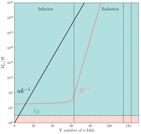
Figure 4: Schematic representation of the evolution of the different physical scales. $a/k$ (black) represents the physical wavelength of the mode $\bm{k}$ under consideration. When $a/k$ crosses $\ell_{E}$ (green dashed), the coherence length of the environment, decoherence starts to be effective. When $a/k$ crosses out $H^{-1}$ (pink), the Hubble radius, the perturbation starts to be amplified.

5.2.1 Covariance matrix

With the ansatz (5.10), the integrals appearing in Eqs. (4.17), (4.18) and (4.19) can be performed exactly, and a detailed calculation is presented in Appendix D. In the late-time limit, i.e. on super-Hubble scales, $-k\eta\rightarrow 0$, they can be approximated by

$$\gamma_{11}\simeq \frac{1}{(-k\eta)^{2}}\left\{1-2\left(\frac{k_{\Gamma}}{k}\right)^{2}\left[B_{11}\left(\frac{k}{k_{*}},p,\ell_{E}H\right)+A_{11}\left(\frac{k}{k_{*}},p\right)(-k\eta)^{8-p}\right]\right\},$$ (5.11)

$$\gamma_{12}\simeq \frac{1}{(-k\eta)^{3}}\left\{1-2\left(\frac{k_{\Gamma}}{k}\right)^{2}\left[B_{12}\left(\frac{k}{k_{*}},p,\ell_{E}H\right)+A_{12}\left(\frac{k}{k_{*}},p\right)\left(-k\eta\right)^{8-p}\right]\right\},$$ (5.12)

$$\gamma_{22}\simeq \frac{1}{(-k\eta)^{4}}\left\{1-2\left(\frac{k_{\Gamma}}{k}\right)^{2}\left[B_{22}\left(\frac{k}{k_{*}},p,\ell_{E}H\right)+A_{22}\left(\frac{k}{k_{*}},p\right)\left(-k\eta\right)^{8-p}\right]\right\},$$ (5.13)

see Eqs. (D.38), (D.42) and (D.46), where $k_{*}$ denotes the comoving scale that crosses out the Hubble radius at the reference time $\eta_{*}$. One can check that, in the limit $k_{\Gamma}\rightarrow 0$, one recovers the covariance matrix calculated in the absence of an environment, namely Eqs. (5.4). The coefficients $A_{11}$, $B_{11}$, $A_{12}$, $B_{12}$, $A_{22}$ and $B_{22}$ are functions of the parameters $p$ and $\ell_{E}H$ and their explicit expressions can be found in Appendix D.

Let us note that the expression for $\gamma_{11}$ is of observational interest as it gives the relative correction to the power spectrum of the Mukhanov-Sasaki variable, see Eq. (2.20), or of any quantity proportional to the Mukhanov-Sasaki variable such as the curvature perturbation $\zeta$ that is measured on the cosmic microwave background. Upon expanding the expression given for $B_{11}$ in Appendix D in the regime $\ell_{E}H\ll 1$, one obtains

$$B_{11} \simeq\frac{1}{2}\left(\frac{k}{k_{*}}\right)^{p-3}\biggl{(}\frac{\left(\ell_{E}H\right)^{p-4}}{p-4}\left\{1-\frac{p-4}{2}\left(\ell_{E}H\right)\sin\left(\frac{2}{\ell_{E}H}\right)+{\cal O}\left[\left(\ell_{E}H\right)^{2}\right]\right\}$$

$$-\frac{(p-3)(p-6)}{2^{4-p}}\Gamma(2-p)\cos\left(\frac{\pi}{2}p\right)\biggr{)}.$$ (5.14)

It is interesting to notice that, at next-to-leading order, this expression contains non-analytical terms. However, it is likely that this non-analytical behaviour would be smoothed out if a non-sharp window function were used. On the other hand, we also have $A_{11}=-2(k/k_{*})^{p-3}/[(p-8)(p-5)(p-2)]$, see Eq. (D.31). Which term dominates in $B_{11}$ depends on the relative position of $p$ with respect to $4$, while which of the corrections in Eq. (5.11) dominates depends on whether $p<8$ or $p>8$. There are therefore three cases to distinguish, and one finds

$$\frac{\Delta\mathcal{P}_{\zeta}}{\mathcal{P}_{\zeta}}\simeq\begin{cases}\displaystyle\frac{\left(\ell_{E}H\right)^{p-4}}{4-p}\left(\frac{k_{\Gamma}}{k_{*}}\right)^{2}\left(\frac{k}{k_{*}}\right)^{p-5}\quad&\text{if}\quad p<4,\\ \displaystyle 2^{p-4}(3-p)(6-p)\Gamma(2-p)\cos\left(\frac{\pi p}{2}\right)\left(\frac{k_{\Gamma}}{k_{*}}\right)^{2}\left(\frac{k}{k_{*}}\right)^{p-5}\quad&\text{if}\quad 4<p<8,\\ \displaystyle\frac{4}{(p-8)(p-5)(p-2)}\left(\frac{k_{\Gamma}}{k_{*}}\right)^{2}\left(\frac{k}{k_{*}}\right)^{3}\left(\frac{\eta}{\eta_{*}}\right)^{8-p}\quad&\text{if}\quad p>8.\end{cases}$$ (5.15)

One can check that these expressions coincide with the result obtained in Ref. [19]. In particular, when $p<8$, the correction to the power spectrum freezes on large scale and is scale invariant when $p=5$, while it continues to increase on large scales for $p>8$. These formulas allow one to set upper bound on $\Gamma$ such that the modifications to observables remain negligible, see the white dotted line in Fig. 6 below.

5.2.2 State purity

Endowed with the above expressions of the components $\gamma_{11}$, $\gamma_{12}$ and $\gamma_{22}$ of the covariance matrix, we are now in a position to calculate $\sigma(0)$ and the state purity. However, upon evaluating $\sigma(0)$ by plugging Eqs. (5.11)-(5.13) into Eq. (2.27), one can see that the terms controlled by $k_{\Gamma}$ all cancel out when $\theta=0$, which implies that Eqs. (5.11)-(5.13) must be expanded to higher order in order to get the first correction to $\sigma(0)$. Before following that route, let us note that such an expansion can be avoided by using Eq. (4.13) directly. The right hand side of this equation is proportional to $k_{\Gamma}^{2}$, so it is enough to evaluate it by using the solution (5.4) for $\gamma_{11}$ in the free theory, which leads to

$$\sigma^{2}(0)=\det\gamma^{s}\simeq 1-2\left(\frac{k_{\Gamma}}{k_{*}}\right)^{2}\left(\frac{k}{k_{*}}\right)^{p-5}\int_{1/(\ell_{E}H)}^{-k\eta}\left(y^{3-p}+y^{1-p}\right)\mathrm{d}y,$$ (5.16)

namely

$$\sigma^{2}(0)\simeq 1+2\left(\frac{k_{\Gamma}}{k_{*}}\right)^{2}\left(\frac{k}{k_{*}}\right)^{p-5}\left[\frac{1}{p-2}\left(\frac{k}{k_{*}}\right)^{2-p}\left(\frac{a_{*}}{a}\right)^{2-p}-\frac{\left(\ell_{E}H\right)^{p-4}}{p-4}\right],$$ (5.17)

where we have kept the leading terms in $\ell_{E}H$ and in $-k\eta$ only. This again coincides with the result found in Ref. [19], see Eq. (4.6) of that reference, and it implies that decoherence occurs at the pivot scale $k_{*}$ when

$$\frac{k_{\Gamma}}{k_{*}}\gg\begin{cases}\displaystyle\left(\ell_{E}H\right)^{2-\frac{p}{2}}\qquad&\text{if}\qquad p<2,\\ \displaystyle\left(\frac{a}{a_{*}}\right)^{1-\frac{p}{2}}\qquad&\text{if}\qquad p>2,\end{cases}$$ (5.18)

where we recall that the state purity is related to $\sigma(0)$ via Eq. (2.26). This domain is delineated by the white dashed line in Fig. 6.

Before moving on and addressing the calculation of quantum discord, let us note that the above result can be recovered from a higher-order expansion of the covariance matrix. This is done in detail in Appendix D, see Eqs. (D.2), (D.2) and (D.2). This leads to expressions for $\gamma_{11}$, $\gamma_{12}$ and $\gamma_{22}$ which, compared to Eqs. (5.11), (5.12) and (5.13), contain extra coefficients (i.e. beyond $A_{11}$, $B_{11}$, $A_{12}$, $B_{12}$, $A_{22}$ and $B_{22}$), namely $C_{11}$, $D_{11}$, …, $C_{12}$, $D_{12}$, …and $C_{22}$, $D_{22}$, …, the explicit expressions of which are given in Appendix D. Of course, these coefficients are also functions of the parameters $p$ and $\ell_{E}H$. Plugging the result into Eq. (2.27), one obtains that, on super-Hubble scales,

$$\sigma^{2}(0) =\Sigma_{-6}\left(-k\eta\right)^{-6}+\Sigma_{-5}\left(-k\eta\right)^{-5}+\Sigma_{-4}\left(-k\eta\right)^{-4}+\Sigma_{-3}\left(-k\eta\right)^{-3}+\Sigma_{-2}\left(-k\eta\right)^{-2}$$

$$+\Sigma_{-1}\left(-k\eta\right)^{-1}+1+\Sigma_{0}+\Sigma_{1}\left(-k\eta\right)+\cdots+\Sigma_{2-p}\left(-k\eta\right)^{2-p}+\Sigma_{4-p}\left(-k\eta\right)^{4-p}$$

$$+\Sigma_{5-p}\left(-k\eta\right)^{5-p}+\cdots.$$ (5.19)

Each coefficient $\Sigma_{i}$ is a combination of the coefficients $A_{11}$, $B_{11}$, …, $A_{12}$, $B_{12}$, …and $A_{22}$, $B_{22}$ …. As a consequence, the $\Sigma_{i}$’s are also functions of the parameters $p$ and $\ell_{E}H$ and are proportional to $k_{\Gamma}^{2}$ or $k_{\Gamma}^{4}$, which guarantees that, without an environment (i.e. when $k_{\Gamma}\rightarrow 0$), one recovers $\sigma(0)=1$. Then, using the explicit expressions of $A_{11}$, $B_{11}$, …, $A_{12}$, $B_{12}$, …and $A_{22}$, $B_{22}$ …given in Appendix D, one can show that $\Sigma_{-6}=\Sigma_{-5}=\Sigma_{-4}=\Sigma_{-3}=\Sigma_{-2}=\Sigma_{-1}=\Sigma_{1}=\cdots=0$. These relationships are direct consequences of the cancellations mentioned before, and indicate that the expansion has to be performed to very high order indeed. Therefore, at leading order in the super-Hubble limit, one has

$$\sigma^{2}(0)\simeq 1+\Sigma_{0}+\Sigma_{2-p}\left(-k\eta\right)^{2-p}+\cdots,$$ (5.20)

with

$$\Sigma_{0} =\left(\frac{k_{\Gamma}}{k}\right)^{2}\left(-2C_{11}+4E_{12}-2E_{22}-2F_{11}-2G_{22}\right)$$

$$+\left(\frac{k_{\Gamma}}{k}\right)^{4}\left(-4C_{12}^{2}+4D_{11}D_{22}-8B_{12}E_{12}+4C_{11}E_{22}+4B_{22}F_{11}+4B_{11}G_{22}\right),$$ (5.21)

$$\Sigma_{2-p} =\left(\frac{k_{\Gamma}}{k}\right)^{2}\left(-2A_{11}+4A_{12}-2A_{22}\right)+\left(\frac{k_{\Gamma}}{k}\right)^{4}\left(4A_{22}B_{11}-8A_{12}B_{12}+4A_{11}B_{22}\right)\,.$$ (5.22)

As mentioned above, the coefficients appearing in the expansions of $\gamma_{11}$, $\gamma_{12}$ and $\gamma_{22}$ are functions of $p$ and $\ell_{E}H$. However, the coefficients $A_{11}$, $A_{12}$ and $A_{22}$ only depend on $p$, see the explicit expressions in Appendix D, Eqs. (D.31), (D.41) and (D.45). It follows that the term proportional to $k_{\Gamma}^{2}$ in the expression of $\Sigma_{2-p}$ is also a function of $p$ only. Explicitly, one has

$$-2A_{11}+4A_{12}-2A_{22}=\frac{2}{p-2}\left(\frac{k}{k_{*}}\right)^{p-3}\,.$$ (5.23)

By contrast, the term proportional to $k_{\Gamma}^{2}$ in the coefficient $\Sigma_{0}$ contains the terms $C_{11}$, $E_{12}$, $E_{22}$, $F_{11}$ and $G_{22}$ and, as consequence, depends on $p$ but also on $\ell_{E}H$. Explicitly, one finds

$$-2C_{11}+4E_{12}-2E_{22}-2F_{11}-2G_{22}=-2\left(\frac{k}{k_{*}}\right)^{p-3}\left[\frac{\left(\ell_{E}H\right)^{p-4}}{p-4}+\frac{\left(\ell_{E}H\right)^{p-2}}{p-2}\right].$$ (5.24)

Combining the above results, one recovers Eq. (5.17), which is an important consistency check of our calculations.

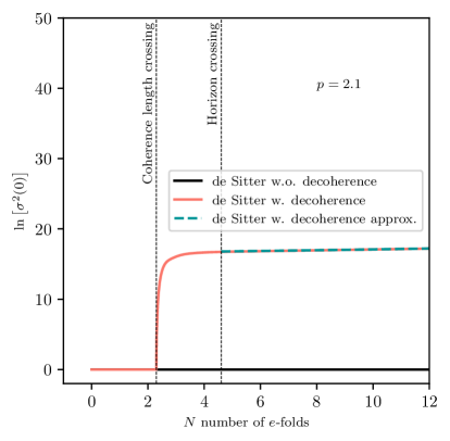
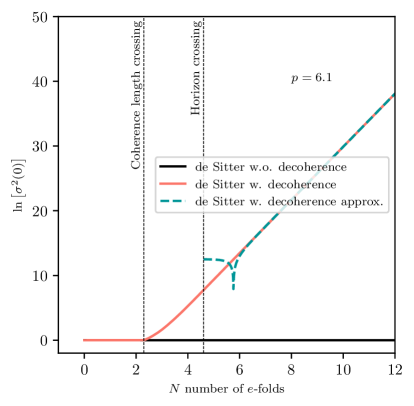
Figure 5: $\ln\left[\sigma^{2}(0)\right]$ with (pink) and without (black) decoherence for the de Sitter case. The approximated version (green dashed) is obtained using Eq. (5.20) for $\sigma^{2}(0)$. The first vertical dashed line shows the time when the mode $\bm{k}$ starts to decohere $\ell_{E}a/k=1$, the second the time when the mode $\bm{k}$ exits the Hubble radius. The parameters are $\ell_{E}H=0.1$, $x_{\star}=1$, $p=2.1$ (left) or $p=6.1$ (right), and $k_{\Gamma}/k=10$.

5.2.3 Quantum discord

The final step is to calculate $\sigma^{2}(\theta)$ and extract quantum discord. Given that we already have computed $\sigma^{2}(0)$, see Eq. (5.17), and since Eq. (2.27) can be rewritten as

$$\sigma(\theta)=\mathchoice{{\hbox{$\displaystyle\sqrt{\sigma^{2}(0)+\frac{1}{4}\left[\left(\gamma_{11}-\gamma_{22}\right)^{2}+4\gamma_{12}^{2}\right]\sin^{2}\left(2\theta\right)\,}$}\lower 0.4pt\hbox{\vrule height=9.66666pt,depth=-7.73337pt}}}{{\hbox{$\textstyle\sqrt{\sigma^{2}(0)+\frac{1}{4}\left[\left(\gamma_{11}-\gamma_{22}\right)^{2}+4\gamma_{12}^{2}\right]\sin^{2}\left(2\theta\right)\,}$}\lower 0.4pt\hbox{\vrule height=9.30444pt,depth=-7.44359pt}}}{{\hbox{$\scriptstyle\sqrt{\sigma^{2}(0)+\frac{1}{4}\left[\left(\gamma_{11}-\gamma_{22}\right)^{2}+4\gamma_{12}^{2}\right]\sin^{2}\left(2\theta\right)\,}$}\lower 0.4pt\hbox{\vrule height=6.53888pt,depth=-5.23112pt}}}{{\hbox{$\scriptscriptstyle\sqrt{\sigma^{2}(0)+\frac{1}{4}\left[\left(\gamma_{11}-\gamma_{22}\right)^{2}+4\gamma_{12}^{2}\right]\sin^{2}\left(2\theta\right)\,}$}\lower 0.4pt\hbox{\vrule height=5.03888pt,depth=-4.03113pt}}},$$ (5.25)

we see that we only need to estimate the second term, i.e. the one proportional to $\sin^{2}(2\theta)$. This is easier since no cancellation occurs in that term. In Appendix D, we find that the dominant contribution comes from $\gamma_{22}$, and that $(\gamma_{11}-\gamma_{22})^{2}+4\gamma_{12}^{2}\simeq(-k\eta)^{-8}[1-({k_{\Gamma}}/{k})^{2}B_{11}/2]^{2}$, see Eqs. (D.38), (D.42) and (D.46). This leads to

$$\sigma^{2}(\theta) =\left[1-\frac{1}{2}\left(\frac{k_{\Gamma}}{k}\right)^{2}B_{11}\right]^{2}\frac{\sin^{2}(2\theta)}{4\left(-k\eta\right)^{8}}+\mathcal{O}\left[\left(-k\eta\right)^{-6}\right]\,.$$ (5.26)

Recalling that $B_{11}$ does not depend on time, one can see that the effect of the environment is only to change the prefactor in $\sigma(\theta)$, while it does not affect its time behaviour $\sigma(\theta)\propto(k\eta)^{-4}$ on super-scales.

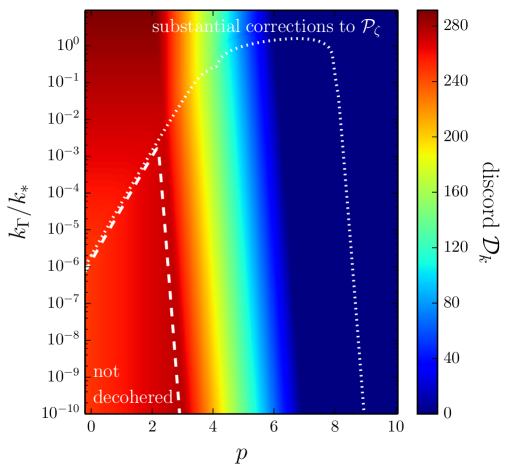
Figure 6: Quantum discord $\mathcal{D}_{k}$ as a function of $p$ and $k_{\Gamma}/k_{*}$, for $k=k_{*}$, $-k\eta=e^{-50}$ (corresponding to the scales probed in the cosmic microwave background at the end of inflation), $\ell_{E}H=10^{-3}$ and $\theta=-\pi/4$. The white dashed line is the contour line of $\mathrm{Tr}(\rho^{2})=1/2$, and above that line the quantum state is decohered. The white dotted line is the contour line of $\Delta\mathcal{P}_{\zeta}/\mathcal{P}_{\zeta}=1$, above which the power spectrum is spoilt by environmental effects. These two contours essentially correspond to Fig. 6 of Ref. [19]; but, in Fig. 6 of Ref. [19], the region where there is a substantial change of the spectral index is displayed, as opposed to the region where there is a substantial change of $\mathcal{P}_{\zeta}$ in the above figure. This is the reason why, in Fig. 6 of Ref. [19], there is a feature at $p=5$, for which the corrections are scale-invariant, which does not appear in the above figure. One of the main result of the present paper is the value of the quantum discord in the parameter space $(p,k_{\Gamma}/k_{*})$. Let us also notice that the “not decohered” region invades the whole figure for sufficiently small values of $k_{\Gamma}$. Here, it looks bounded because, due to the logarithmic scale used, $k_{\Gamma}$ is “cut” at $k_{\Gamma}/k_{*}=10^{-10}$.

Let us now consider the ratio $\sigma^{2}(0)/\sigma(\theta)$ which, as explained in Sec. 4.4, determines the fate of quantum discord. If $p<2$, the second term dominates in Eq. (5.17), hence $\sigma^{2}(0)$ reaches a constant on large scales. One thus has $\sigma^{2}(0)/\sigma(\theta)\propto a^{-4}$, which is highly suppressed on super-Hubble scales, and which gives rise to $\mathcal{D}_{k}\propto 4\log_{2}[a/a(k)]$. This shows that quantum discord is large in that case, and one recovers the result obtained in Eq. (5.9). If $p\geq 2$, the first term dominates in Eq. (5.17), hence $\sigma^{2}(0)\propto a^{p-2}$ on super-Hubble scales. As a consequence, $\sigma^{2}(0)/\sigma(\theta)\propto a^{p-6}$, the time behaviour of which depends on whether $p<6$ or $p>6$ as illustrated by Fig. 5 . If $p<6$, $\sigma^{2}(0)/\sigma(\theta)$ decays, and one has $\mathcal{D}_{k}\propto(6-p)\log_{2}[a/a(k)]$, so the discord remains large. If $p>6$, $\sigma^{2}(0)/\sigma(\theta)$ increases on super-Hubble scales, and upon expanding Eq. (2.28) in that regime one finds that $\mathcal{D}_{k}\propto[a/a(k)]^{6-p}$, so it becomes highly suppressed. The behaviour of $\mathcal{D}_{k}$ on each side of the threshold is illustrated by Fig. 7

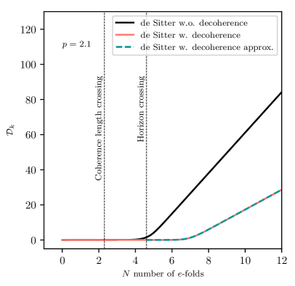
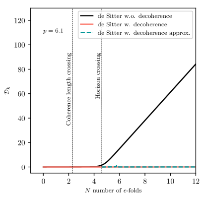
Figure 7: Quantum discord $\mathcal{D}_{k}$ with (pink) and without (black) decoherence for the de Sitter case. The approximated version (green dashed) is obtained using the first order approximations (5.11), (5.12) and (5.13) for $\gamma_{ij}$ and the expression (5.20) for $\sigma^{2}(0)$ to obtain $\sigma^{2}(\theta)$ in (5.25). The quantity $\sigma^{2}(0)$ and $\sigma^{2}(\theta)$ are then used in the expression (2.28) for the discord. The first vertical dashed line shows the time when the mode $\bm{k}$ starts to decohere $\ell_{E}a/k=1$, the second the time when the mode $\bm{k}$ exits the Hubble radius. The parameters are $\ell_{E}H=0.1$, $x_{\star}=1$, $p=2.1$ (left) or $p=6.1$ (right), and $k_{\Gamma}/k=10$.

These considerations can be checked in Fig. 6, where quantum discord is displayed as a function of $p$ and $k_{\Gamma}/k_{*}$. It confirms that the pivotal value of $p$ from the point of view of quantum discord is $p=6$: discord remains large on super-Hubble scales when $p<6$, and is highly suppressed otherwise. Note however that the above formulas only describe the time behaviour at large scales, and do not incorporate the constant prefactors that can otherwise be readily established from combining the above results. These prefactors depend on both $\ell_{E}H$ and $\Gamma$ (through $k_{\Gamma}$), and they explain why the discord shown in Fig. 6 does not depend only on $p$ (for instance, even for $p>6$, one can get a substantial discord by considering extremely low values of $k_{\Gamma}$, in agreement with the fact that in the limit $\Gamma\to 0$, one recovers the results of Sec. 5.1). Nonetheless, for reasonable values of the coupling constant $\Gamma$, the result is mostly determined by the value of $p$.

In Fig. 6, we have also displayed the region in parameter space where decoherence does not occur (below the white dashed line, see Sec. 5.2.2) and the region where substantial corrections to the power spectrum are obtained (above the white dotted line, see Sec. 5.2.1). One can see that when the coupling to the environment is not strong enough to make the system decohere, quantum discord is always large on super-Hubble scales. This corresponds to the bottom left corner in Fig. 6. In the opposite corner, namely the top-right region in Fig. 6, the coupling with the environment is so strong that it both decoheres the system very efficiently, while it prevents its quantum discord from growing. An important remark is that, between these two regimes, there are regions where quantum discord remains large even though the system decoheres and even when imposing that the observed power spectrum is unaffected by environmental effects.

6 Conclusions

In this work, we have studied how quantum discord behaves in the presence of an environment. When a quantum system couples to environmental degrees of freedom, the entanglement between the open system and the environment leads to decoherence of the system, which is usually associated with the loss of certain quantum features displayed by the system. Since discord characterises how “genuinely quantum” the correlations between subparts of the system are, it is naturally expected that decoherence leads to a suppression of discord. The goal of this work was to study this effect on generic grounds, since any practical experiment aiming at revealing the presence of quantum effects is a priori subject to such environmental limitations.

For simplicity, we have considered the case of a quantum scalar field with (homogeneous and isotropic) quadratic Hamiltonian, which boils down to a collection of independent pairs of quantum parametric oscillators, one for each pair of opposite Fourier modes. We have shown that, in general, quantum discord depends on the precise way these systems are partitioned into two subsystems. We have found a generic parameterisation that describes all possible partitions, which has allowed us to derive quantum discord for any partitioning. Note that the way a given physical system should be split into two subsystems is sometimes obvious: for instance, for two particles located in each polariser of a Bell’s inequality experiment, the two sub-systems are clearly the two space-like separated particles. However, the Fourier sub-sector of a quantum field does not feature such a clear preferred partitioning, and it is therefore necessary to study how the result depends on the partition in general.

In the absence of interactions with an environment, the system is placed in a Gaussian state known as the two-mode squeezed state, which can be equivalently described in terms of Bogoliubov coefficients, squeezing parameters, or covariance matrix. In that case, we recovered the formula derived in Ref. [5] for quantum discord, which we nonetheless extended to any partitioning.

In the case where an environment is present and couples to the system, for explicitness, we have assumed that the coupling is linear in the phase-space variables describing the system, and that it can be cast in terms of a Lindblad equation (this is the so-called Caldeira-Leggett model). In this context, the state remains Gaussian (though not pure anymore), so it can still be described in terms of a covariance matrix, for which we have derived the modified evolution equation. We have shown that generalised squeezing parameters can also still be defined, from their geometrical phase-space interpretation. A third parameter describing the area of the elliptic contours of the Wigner function should be added to the usual squeezing amplitude and squeezing angle, which respectively correspond to the eccentricity and orientation of these ellipses. This “third squeezing parameter” equals one for a pure state and is larger than one otherwise, and it is directly related to the inverse purity of the state. We have thus derived the modified evolution equations for these three “squeezing parameters”, which represent an alternative description of the state with an intuitive geometrical interpretation [41].

We have then computed quantum discord in this model, both in terms of the covariance matrix and in terms of the generalised squeezing parameters. As in the case of pure states, we have found that quantum discord does not depend on the squeezing angle, but only involves the squeezing amplitude, the state purity and the partition parameters. More precisely, in a given partitioning, quantum discord increases as the length of the semi-minor axis of the phase-space ellipse decreases, which provides a simple geometrical interpretation of discord. This implies that discord increases with both the squeezing amplitude and the state purity. In general, as the time evolution proceeds, the squeezing amplitude increases (denoting particle creation) and the state purity decreases (because of decoherence), so the two effects compete. The details of how quantum discord is affected by an environment thus depend on the rate at which these two parameters vary, which has to be discussed on a model-by-model basis. Those findings are consistent with the work of Ref. [18] where the authors considered a model corresponding to p=5 in our parametrisation. They computed an upper bound on the discord which despite decoherence grows in time, albeit at a reduced rate, in line with the discussion of Sec. 5.2.3.

To go beyond those generic considerations, we have finally applied our framework to the case of primordial cosmological perturbations. This case study is of particular interest not only because it provides a useful illustration of the tools introduced in this work, but also since the possible presence of quantum correlations in cosmic structures, and the potential of decoherence to make them undetectable, is of great importance for our understanding of their origin. Assuming that the coupling parameter $\Gamma$ between the system (here cosmological perturbations) and the environment (possibly heavier fields, smaller-scale degrees of freedom, etc.) grows as a power of the scale factor $a$ of the universe, $\Gamma\propto a^{p}$, whether or not decoherence leads to a suppression of discord (i.e. whether or not the phase-space semi-minor axis increases) crucially depends on $p$. More precisely, if $p<6$, discord remains large on large scales, and is strongly suppressed otherwise. Let us also note that for $p<2$, decoherence cannot proceed without substantially affecting the observed power spectrum of the cosmological density field, so in the region of parameter space that is in agreement with current observations, environmental effects are mostly irrelevant. For $2<p<6$, there exists a regime where the state decoheres but remains strongly discordant, while preserving its power spectrum.

Those considerations imply that there is no simple relationship between decoherence and discord: one can find situations where the state of the system becomes decohered and non-discordant, where it becomes decohered but remains discordant, where it remains pure and discordant, or where it is pure and non discordant (this case does not appear in cosmology but may be encountered in other contexts, see the discussion around Fig. 2). As a consequence, although decoherence may affect our ability to reveal the presence of quantum correlations within a given quantum system, this effect cannot be simply assessed by considering the amount of decoherence (i.e. the state purity). One alternative criterion may be the quantum discord discussed in this work, although its relationship with concrete observables is not clear, in particular in the context of mixed states [42]. This is why a next natural step would be to apply the present framework to investigate violations of Bell-inequalities in the presence of environmental effects, using the techniques developed in Refs. [43, 44, 17, 45, 46]. In this way, one may be able to better understand the relationship between discord, decoherence, Bell inequalities violation, and maybe other criteria such as Peres-Horodecki separability [47], in a broad context.

Appendix A Partitions

As explained in Sec. 2.2, when studying the nature of the correlations present within a given (classical or quantum) system, one first has to split this system into two (or more) sub-systems, and then to analyse how these sub-systems are correlated. This way to divide the system into several sub-systems is called a “partition”, and in this appendix we formally study how partitions can be defined on generic grounds, and how different partitions are related to each other.

A.1 Quantum phase space

In this article, we consider continuous-variable systems, i.e. systems described by Hermitian operators satisfying canonical commutation relation. It can be, for instance, the positions $\hat{q}_{i}$ and momenta $\hat{\pi}_{i}$ of $n$ particles (with $i=1\cdots n$), with $[\hat{q}_{i},\hat{\pi}_{j}]=i\delta_{ij}$. This can also correspond to the Fourier modes of a quantum field, see Sec. 2.1. The quantum state of the system is an element of the Hilbert space

$${\mathcal{E}}=\bigotimes_{i=1\,\cdots\,n}{\mathcal{E}}_{i}\,,$$ (A.1)

where ${\mathcal{E}}_{i}$ is the Hilbert space associated to the $i^{\mathrm{th}}$ particle. It can be described by the vector

$$\hat{R}=(\hat{q}_{1},\hat{\pi}_{1},\cdots,\hat{q}_{i},\hat{\pi}_{i},\cdots,\hat{q}_{n},\hat{\pi}_{n})^{\mathrm{T}}\,.$$ (A.2)

In terms of the components of the vector $\hat{R}$, the commutation relations can be written as

$$\left[\hat{R}_{a},\hat{R}_{b}\right]=iJ_{ab}^{(n)}\,,$$ (A.3)

where $J^{(n)}$ is the $2n\times 2n$ block-diagonal matrix

$$J^{(n)}=\left(\begin{array}[]{ccc}J^{(1)}&&\\ &\ddots&\\ &&J^{(1)}\end{array}\right)\quad\text{with}\quad J^{(1)}=\begin{pmatrix}0&1\\ -1&0\end{pmatrix}\,.$$ (A.7)

An alternative description of the system is by means of the creation and annihilation operators $\hat{c}_{i}$ and $\hat{c}_{i}^{\dagger}$, defined by

$$\hat{q}_{i}=\frac{1}{\mathchoice{{\hbox{$\displaystyle\sqrt{2\,}$}\lower 0.4pt\hbox{\vrule height=6.44444pt,depth=-5.15558pt}}}{{\hbox{$\textstyle\sqrt{2\,}$}\lower 0.4pt\hbox{\vrule height=6.44444pt,depth=-5.15558pt}}}{{\hbox{$\scriptstyle\sqrt{2\,}$}\lower 0.4pt\hbox{\vrule height=4.51111pt,depth=-3.6089pt}}}{{\hbox{$\scriptscriptstyle\sqrt{2\,}$}\lower 0.4pt\hbox{\vrule height=3.22221pt,depth=-2.57779pt}}}}\left(\hat{c}_{i}+\hat{c}_{i}^{\dagger}\right),\quad\hat{\pi}_{i}=-\frac{i}{\mathchoice{{\hbox{$\displaystyle\sqrt{2\,}$}\lower 0.4pt\hbox{\vrule height=6.44444pt,depth=-5.15558pt}}}{{\hbox{$\textstyle\sqrt{2\,}$}\lower 0.4pt\hbox{\vrule height=6.44444pt,depth=-5.15558pt}}}{{\hbox{$\scriptstyle\sqrt{2\,}$}\lower 0.4pt\hbox{\vrule height=4.51111pt,depth=-3.6089pt}}}{{\hbox{$\scriptscriptstyle\sqrt{2\,}$}\lower 0.4pt\hbox{\vrule height=3.22221pt,depth=-2.57779pt}}}}\left(\hat{c}_{i}-\hat{c}_{i}^{\dagger}\right).$$ (A.8)

They can be assembled into the vector

$$\hat{C}=(\hat{c}_{1},\cdots,\hat{c}_{i},\cdots,\hat{c}_{n},\hat{c}_{1}^{\dagger},\cdots,\hat{c}_{i}^{\dagger},\cdots,\hat{c}_{n}^{\dagger})^{\mathrm{T}}\,.$$ (A.9)

Contrary to the vector $\hat{R}$, notice that $\hat{C}$ is not arranged such that the variables describing the subsystem $i$ directly follow each other, and the reason for this choice will be made clear below.

The relation between $\hat{R}$ and $\hat{C}$ is linear and can thus be written in matricial form as $\hat{R}=M^{(n)}\cdot\hat{C}$, where $M^{(n)}$ is an unitary matrix that can be obtained from Eq. (A.8). For instance, with $n=2$, one has

$$M^{(2)}=\frac{1}{\mathchoice{{\hbox{$\displaystyle\sqrt{2\,}$}\lower 0.4pt\hbox{\vrule height=6.44444pt,depth=-5.15558pt}}}{{\hbox{$\textstyle\sqrt{2\,}$}\lower 0.4pt\hbox{\vrule height=6.44444pt,depth=-5.15558pt}}}{{\hbox{$\scriptstyle\sqrt{2\,}$}\lower 0.4pt\hbox{\vrule height=4.51111pt,depth=-3.6089pt}}}{{\hbox{$\scriptscriptstyle\sqrt{2\,}$}\lower 0.4pt\hbox{\vrule height=3.22221pt,depth=-2.57779pt}}}}\begin{pmatrix}1&0&1&0\\ -i&0&i&0\\ 0&1&0&1\\ 0&-i&0&i\end{pmatrix}.$$ (A.16)

The commutation relations can be expressed as

$$\left[\hat{C}_{a},\hat{C}_{b}\right]=\Omega_{ab}^{(n)}\,,$$ (A.17)

with $\Omega^{(n)}=iM^{(n),-1}\cdot J^{(n)}\cdot M^{(n),-1,\mathrm{T}}$, i.e.

$$\Omega^{(n)}=\begin{pmatrix}0&\mathbb{I}_{n}\\ -\mathbb{I}_{n}&0\end{pmatrix},$$ (A.18)

where $\mathbb{I}_{n}$ is the identity matrix of size $n$.

A.2 Partitioning

For $n\geq 2$, the degrees of freedom can always be split into two subsets $A$ and $B$. This defines a partition and allows us to see the whole system as a bipartite system. An important point is that one can define several partitions for the same system. As an introductory (and elementary) example, let us consider the case $n=4$ where $\hat{R}=(\hat{q}_{1},\hat{\pi}_{1},\hat{q}_{2},\hat{\pi}_{2},\hat{q}_{3},\hat{\pi}_{3},\hat{q}_{4},\hat{\pi}_{4})^{\mathrm{T}}$. For instance, one can choose the subsystem $A$ to be made of the first two degrees of freedom and to be described by $\hat{R}^{(A)}=(\hat{q}_{1},\hat{\pi}_{1},\hat{q}_{2},\hat{\pi}_{2})^{{\mathrm{T}}}$, and the subsystem $B$ to contain the third and fourth degrees of freedom, $\hat{R}^{(B)}=(\hat{q}_{3},\hat{\pi}_{3},\hat{q}_{4},\hat{\pi}_{4})^{{\mathrm{T}}}$. Then, the vector $\hat{R}$ can be written as $\hat{R}=(\hat{R}^{(A)},\hat{R}^{(B)})^{{\mathrm{T}}}$. This definition of $\hat{R}$, namely the way we order its components, is, implicitly, a definition of a partition. Obviously, other partitions are possible, for instance the one defined by $\hat{R}^{(A)}{}^{\prime}=(\hat{q}_{1},\hat{\pi}_{1},\hat{q}_{3},\hat{\pi}_{3})^{{\mathrm{T}}}$ and $\hat{R}^{(B)}{}^{\prime}=(\hat{q}_{2},\hat{\pi}_{2},\hat{q}_{4},\hat{\pi}_{4})^{{\mathrm{T}}}$ with $\hat{R}^{\prime}=(\hat{R}^{(A)}{}^{\prime},\hat{R}^{(B)}{}^{\prime})^{{\mathrm{T}}}$.

More generally, changing the partition can be viewed as performing a canonical transformation on the system (i.e. a transformation that preserves the commutator structure). A linear canonical transformation is a transformation $\hat{R}\rightarrow\hat{R}^{\prime}=T\hat{R}$, where $T$ is a real matrix since $\hat{R}$ and $\hat{R}^{\prime}$ are Hermitian, which preserves the commutators, i.e. such that $[\hat{R}^{\prime}_{a},\hat{R}^{\prime}_{b}]=[\hat{R}_{a},\hat{R}_{b}]$ (hereafter we drop the index $n$ for notational convenience). This leads to the condition

$$TJT^{{\mathrm{T}}}=J\,,$$ (A.19)

which defines the group of symplectic matrices $T$ [48, 24, 49]. In particular, any symplectic matrix has determinant $1$ [48],

$$\det T=1\,.$$ (A.20)

In the simple example mentioned above, one can check that the transformation matrix $T$ is indeed symplectic. Let us note that canonical transformations can also be defined at the level of the vectors $\hat{C}$, since $\hat{R}\rightarrow T\hat{R}$ leads to $\hat{C}\rightarrow S\hat{C}$ with

$$S=M^{-1}TM=M^{\dagger}TM$$ (A.21)

(where, in the last equation, we have used that $M$ is unitary, see footnote 9). Using the definition of $\Omega$ given below Eq. (A.17), Eqs. (A.19) and (A.21) lead to the condition

$$S\Omega S^{\mathrm{T}}=\Omega\,,$$ (A.22)

which also implies that

$$\det S=1\,.$$ (A.23)

Another useful property for the matrix $S$ comes from the ordering of the entries of the vector $\hat{C}$ in Eq. (A.9), which leads to $\hat{C}^{\dagger}=A\cdot\hat{C}$, where $\hat{C}^{\dagger}$ is defined as $(\hat{C}^{\dagger})_{a}=(\hat{C}_{a})^{\dagger}$ and where $A=\left(\begin{array}[]{cc}0&\mathbb{I}_{n}\\ \mathbb{I}_{n}&0\end{array}\right)$. Since $\hat{R}^{\dagger}=\hat{R}$, the adjoint of the relation $\hat{R}=M\hat{C}$ gives rise to $M^{*}A=M$. Evaluating the complex conjugate of $S=M^{-1}TM$, this leads to

$$S^{*}=ASA\,,$$ (A.24)

where we have used that $A^{2}=\mathbb{I}_{n}$ and that $T^{*}=T$ (since $\hat{R}$ and $\hat{R}^{\prime}$ are both Hermitian).

It is worth pointing out that there are canonical transformations that do not mix the two subsystems (they are called “local” transformations) and hence do not change the partition. A simple example is $\hat{R}^{\prime}=(\hat{q}_{2},\hat{\pi}_{2},\hat{q}_{1},\hat{\pi}_{1},\hat{q}_{3},\hat{\pi}_{3},\hat{q}_{4},\hat{\pi}_{4})^{\mathrm{T}}$ where we have simply flipped the ordering of the two first degrees of freedom. As a less trivial example, let us define $\hat{Q}_{ij}^{\pm}=(\hat{q}_{i}\pm\hat{q}_{j})/\mathchoice{{\hbox{$\displaystyle\sqrt{2\,}$}\lower 0.4pt\hbox{\vrule height=6.44444pt,depth=-5.15558pt}}}{{\hbox{$\textstyle\sqrt{2\,}$}\lower 0.4pt\hbox{\vrule height=6.44444pt,depth=-5.15558pt}}}{{\hbox{$\scriptstyle\sqrt{2\,}$}\lower 0.4pt\hbox{\vrule height=4.51111pt,depth=-3.6089pt}}}{{\hbox{$\scriptscriptstyle\sqrt{2\,}$}\lower 0.4pt\hbox{\vrule height=3.22221pt,depth=-2.57779pt}}}$ and $\hat{\Pi}_{ij}^{\pm}=(\hat{\pi}_{i}\pm\hat{\pi}_{j})/\mathchoice{{\hbox{$\displaystyle\sqrt{2\,}$}\lower 0.4pt\hbox{\vrule height=6.44444pt,depth=-5.15558pt}}}{{\hbox{$\textstyle\sqrt{2\,}$}\lower 0.4pt\hbox{\vrule height=6.44444pt,depth=-5.15558pt}}}{{\hbox{$\scriptstyle\sqrt{2\,}$}\lower 0.4pt\hbox{\vrule height=4.51111pt,depth=-3.6089pt}}}{{\hbox{$\scriptscriptstyle\sqrt{2\,}$}\lower 0.4pt\hbox{\vrule height=3.22221pt,depth=-2.57779pt}}}$ so that $[\hat{Q}_{ij}^{\pm},\Pi_{ij}^{\pm}]=i$, thus ensuring that the corresponding transformation can be described by a symplectic matrix. Clearly, $\hat{R}^{\prime}=(\hat{Q}_{12}^{+},\hat{\Pi}_{12}^{+},\hat{Q}_{12}^{-},\hat{\Pi}_{12}^{-},\hat{q}_{3},\hat{\pi}_{3},\hat{q}_{4},\hat{\pi}_{4})^{{\mathrm{T}}}$ corresponds to the same partition as $\hat{R}=(\hat{q}_{1},\hat{\pi}_{1},\hat{q}_{2},\hat{\pi}_{2},\hat{q}_{3},\hat{\pi}_{3},\hat{q}_{4},\hat{\pi}_{4})^{\mathrm{T}}$ since we still have $1$ and $2$ in subsystem $A$ and $3$ and $4$ in subsystem $B$. Therefore, partition changes are described by only a subclass of symplectic matrices (namely those that are not $n$$\times$$n$-block diagonal).

In order for two parameterisations of the system to share the same vacuum state, let us first impose that $S$ does not mix creation and annihilation operators. This implies that $S$ is block diagonal (which is the reason why the ordering made in Eq. (A.9) was indeed convenient). The condition (A.24) then imposes that the two blocks are complex conjugate to each other, so $S$ can be written as

$$S=\begin{pmatrix}s^{(n)}&0\\ 0&s^{(n)}{}^{*}\end{pmatrix}\,.$$ (A.25)

The symplectic condition (A.22) leads to $s^{(n)}{}^{\dagger}s^{(n)}=\mathbb{I}_{n}$, i.e. the matrices $s^{(n)}$ belong to the unitary group $U(n)$. This discussion shows that the space of partitions is essentially the group $U(n)$, so any parameterisation of that group, which has dimension $n^{2}$, leads to a parameterisation of all possible partitions, by means of the above formulas. For instance, with $n=2$, matrices of $U(2)$ can be written in the form

$$s^{(2)}=\begin{pmatrix}e^{i\alpha}\cos\theta&-e^{i\delta}\sin\theta\\ e^{i\beta}\sin\theta&e^{i(\delta+\beta-\alpha)}\cos\theta\end{pmatrix},$$ (A.26)

where $\alpha$, $\beta$, $\delta$ and $\theta$ are four arbitrary real numbers, which thus parameterise all possible partitions. The matrix $T$ can be also written in terms of these parameters by making use of Eq. (A.21) together with Eqs. (A.16) and (A.25), leading to

$$T =\begin{pmatrix}\cos\alpha\cos\theta&-\sin\alpha\cos\theta&-\cos\delta\sin\theta&\sin\delta\sin\theta\\ \sin\alpha\cos\theta&\cos\alpha\cos\theta&-\sin\delta\sin\theta&-\cos\delta\sin\theta\\ \cos\beta\sin\theta&-\sin\beta\sin\theta&\cos(\alpha-\beta-\delta)\cos\theta&\sin(\alpha-\beta-\delta)\cos\theta\\ \sin\beta\sin\theta&\cos\beta\sin\theta&-\sin(\alpha-\beta-\delta)\cos\theta&\cos(\alpha-\beta-\delta)\cos\theta\end{pmatrix}.$$ (A.27)

As a consistency check, one can verify that such a matrix is indeed symplectic, namely that it satisfies Eq. (A.19). However, note that the group of real $4$$\times$$4$ symplectic matrices, usually denoted $\mathrm{Sp}(4,\mathbb{R})$, is of dimension 10 [49]. Therefore, partition changes, that are described by 4 parameters, only correspond to a subgroup (isomorphic to $\mathrm{U}(2)$, and corresponding to the “rotation” generators of table 2 in Ref. [49]) of the symplectic group.

Note that, in agreement with the group structure of $U(n)$, changes of partitions can be composed according to

$$T^{1/2\to 1^{\prime}/2^{\prime}}=T^{1/2\to 1^{\prime\prime}/2^{\prime\prime}}\cdot T^{1^{\prime\prime}/2^{\prime\prime}\to 1^{\prime}/2^{\prime}}\,,$$ (A.28)

and that

$$T^{1/2\to 1^{\prime}/2^{\prime}}=\left(T^{1^{\prime}/2^{\prime}\to 1/2}\right)^{-1}\,,$$ (A.29)

with similar expressions for $S^{1/2\to 1^{\prime}/2^{\prime}}$.

Appendix B Covariance matrix in arbitrary partition

The covariance matrix $\gamma$ in a given phase-space parameterisation $\hat{R}$ is defined by Eq. (2.17). Since $\hat{R}_{a}\hat{R}_{b}=(\{\hat{R}_{a},\hat{R}_{b}\}+[\hat{R}_{a},\hat{R}_{b}])/2$, Eqs. (A.3) and (2.17), give rise to

$$\langle\hat{R}_{a}\hat{R}_{b}\rangle=\frac{1}{2}\gamma_{ab}+\frac{i}{2}J_{ab}^{(n)}\,,$$ (B.1)

where the matrix $J^{(n)}$ has been defined in Eq. (A.7). Furthermore, since $\hat{R}_{a}$ and $\hat{R}_{b}$ are Hermitian, $\{\hat{R}_{a},\hat{R}_{b}\}$ is also Hermitian, and Eq. (2.17) implies that $\gamma$ is a real symmetric matrix. Note that the correlators of the ladder operators introduced in Eq. (A.9), and arranged into the vector $\hat{C}=M^{(n),-1}\hat{R}$, can also be expressed in terms of the covariance matrix:

$$\left\langle\left\{\hat{C}_{a},\hat{C}_{b}\right\}\right\rangle=M^{(n),-1}_{ac}\gamma_{cd}M^{(n),*}_{db}$$ (B.2)

where we have used that $M^{(n)}$ is unitary, see footnote 9.

In the Fourier subspaces of a real scalar field, the covariance matrix is given by Eq. (2.19) in the $\mathrm{R}/\mathrm{I}$ partition. Making use of Eq. (2.16) and (2.18), the covariance matrix can then be computed in all partitions, and one finds

$$\gamma=\begin{pmatrix}\gamma_{A}&\gamma_{C}\\ \gamma_{C}&\gamma_{B}\end{pmatrix},$$ (B.3)

with

$$\gamma_{A} =\begin{pmatrix}\displaystyle\gamma_{11}\cos^{2}\theta+\gamma_{22}\sin^{2}\theta&\displaystyle\gamma_{12}\cos(2\theta)\\ \displaystyle\gamma_{12}\cos(2\theta)&\displaystyle\gamma_{22}\cos^{2}\theta+\gamma_{11}\sin^{2}\theta\end{pmatrix},$$ (B.4)

$$\gamma_{B} =\begin{pmatrix}\displaystyle\gamma_{B}|_{11}&\gamma_{B}|_{12}\\ \displaystyle\gamma_{B}|_{21}&\gamma_{B}|_{22}\end{pmatrix},$$ (B.5)

$$\gamma_{C} =\left(\begin{array}[]{cccc}\displaystyle\frac{1}{2}(\gamma_{11}-\gamma_{22})\sin^{2}(2\theta)+\frac{1}{2}\gamma_{12}\sin(4\theta)&&&\displaystyle-\frac{1}{4}(\gamma_{11}-\gamma_{22})\sin(4\theta)+\gamma_{12}\sin^{2}(2\theta)\\ \displaystyle-\frac{1}{4}(\gamma_{11}-\gamma_{22})\sin(4\theta)+\gamma_{12}\sin^{2}(2\theta)&&&\displaystyle-\frac{1}{2}(\gamma_{11}-\gamma_{22})\sin^{2}(2\theta)-\frac{1}{2}\gamma_{12}\sin(4\theta)\end{array}\right),$$ (B.8)

where the components of $\gamma_{B}$ are given by

$$\gamma_{B}|_{11} =\frac{1}{2}\gamma_{11}+\frac{1}{2}\gamma_{22}+\frac{1}{2}(\gamma_{11}-\gamma_{22})\cos(2\theta)\cos(4\theta)-\gamma_{12}\cos(2\theta)\sin(4\theta),$$ (B.9)

$$\gamma_{B}|_{12} =\gamma_{B}|_{21}=\gamma_{12}\cos(2\theta)\cos(4\theta)+\frac{1}{2}(\gamma_{11}-\gamma_{22})\cos(2\theta)\sin(4\theta),$$ (B.10)

$$\gamma_{B}|_{22} =\frac{1}{2}\gamma_{11}+\frac{1}{2}\gamma_{22}-\frac{1}{2}(\gamma_{11}-\gamma_{22})\cos(2\theta)\cos(4\theta)+\gamma_{12}\cos(2\theta)\sin(4\theta).$$ (B.11)

For instance, recalling that the $\pm\bm{k}$ partition is reached by setting $\theta=\pi/4$, the correlation functions in the “${\bm{k}}$”-sector are given by

$$k\left\langle\hat{q}_{\bm{k}}^{2}\right\rangle =\frac{1}{2}\gamma_{A}|_{11}+\frac{i}{2}J_{11}^{(2)}=\frac{\gamma_{11}+\gamma_{22}}{4}\,,$$ (B.12)

$$\frac{\left\langle\hat{\pi}_{\bm{k}}^{2}\right\rangle}{k} =\frac{1}{2}\gamma_{A}|_{22}+\frac{i}{2}J_{22}^{(2)}=\frac{\gamma_{11}+\gamma_{22}}{4}\,$$ (B.13)

$$\left\langle\hat{q}_{\bm{k}}\hat{\pi}_{\bm{k}}\right\rangle =\gamma_{A}|_{12}+\frac{i}{2}J_{12}^{(2)}=\frac{i}{2},\quad\left\langle\hat{\pi}_{\bm{k}}\hat{q}_{\bm{k}}\right\rangle=\gamma_{A}|_{21}+\frac{i}{2}J_{21}^{(2)}=-\frac{i}{2},$$ (B.14)

and we have the same results in the “$-{\bm{k}}$”-sector since, for $\theta=-\pi/4$, one has $\gamma_{A}=\gamma_{B}=(\gamma_{11}+\gamma_{22})\mathrm{diag}(1,1)/2$. The correlation functions mixing ${\bm{k}}$ and $-{\bm{k}}$ modes depend on the matrix $\gamma_{C}$, and are given by

$$k\left\langle\hat{q}_{\bm{k}}\hat{q}_{-{\bm{k}}}\right\rangle =\frac{1}{2}\gamma_{C}|_{11}+\frac{i}{2}J_{13}^{(2)}=\frac{1}{4}(\gamma_{11}-\gamma_{22})\,$$ (B.15)

$$\frac{1}{k}\left\langle\hat{\pi}_{\bm{k}}\hat{\pi}_{-{\bm{k}}}\right\rangle =\frac{1}{2}\gamma_{C}|_{22}+\frac{i}{2}J_{24}^{(2)}=-\frac{1}{4}(\gamma_{11}-\gamma_{22})\,$$ (B.16)

$$\left\langle\hat{q}_{\bm{k}}\hat{\pi}_{-{\bm{k}}}\right\rangle =\frac{1}{2}\gamma_{C}|_{12}+\frac{i}{2}J_{14}^{(2)}=\frac{1}{2}\gamma_{12},\quad\left\langle\hat{\pi}_{-{\bm{k}}}\hat{q}_{{\bm{k}}}\right\rangle=\frac{1}{2}\gamma_{C}|_{21}+\frac{i}{2}J_{41}^{(2)}=\frac{1}{2}\gamma_{12},$$ (B.17)

$$\left\langle\hat{q}_{-{\bm{k}}}\hat{\pi}_{{\bm{k}}}\right\rangle =\frac{1}{2}\gamma_{C}|_{12}+\frac{i}{2}J_{32}^{(2)}=\frac{1}{2}\gamma_{12},\quad\left\langle\hat{\pi}_{{\bm{k}}}\hat{q}_{-{\bm{k}}}\right\rangle=\frac{1}{2}\gamma_{C}|_{21}+\frac{i}{2}J_{23}^{(2)}=\frac{1}{2}\gamma_{12}\,.$$ (B.18)

Appendix C Quantum discord for Gaussian homogeneous states

In this appendix we explain how the quantum discord can be used as a tool to assess the presence of quantum correlations between two subsystems. In Secs. C.1 and C.2, we first present a brief introduction to the main ideas behind quantum discord and give its mathematical definition. In Secs. C.3 and C.4, we then derive the expression of quantum discord for Gaussian homogeneous states we use in the main text, i.e. Eq. (2.28) .

C.1 Classical correlations

Let us consider two systems $A$ and $B$, and denote by $\{a_{i}\}$ and $\{b_{j}\}$ their possible respective configurations. The probability to find the system $A$ in the configuration $a_{i}$ is noted $p_{i}$, and similarly for $p_{j}$. How uncertain the state of system $A$ is can be characterised by the von Neumann entropy which is defined by the following expression

$$S(A)=-\sum_{i}p_{i}\log_{2}(p_{i})\,.$$ (C.1)

One can check that $S(A)=0$ corresponds indeed to the situation where all $a_{i}$ vanish but one (so the state of A is certain), and that, in general, $S(A)\geq 0$. A similar expression for $S(B)$ can be introduced, and this can also be done for the joint system

$$S(A,B)=-\sum_{i,j}p_{ij}\log_{2}(p_{ij}),$$ (C.2)

where $p_{ij}$ denotes the joint probability to find the system $A$ in configuration $a_{i}$ and the system $B$ in configuration $b_{j}$. Then, the mutual information between $A$ and $B$ can be measured by

$$\mathcal{I}(A,B)=S(A)+S(B)-S(A,B)\,.$$ (C.3)

The fact that $\mathcal{I}(A,B)$ measures the presence of correlations between $A$ and $B$ can be seen by noting that if $A$ and $B$ are uncorrelated, then the mutual information vanishes. Indeed, if $p_{ij}=p_{i}p_{j}$, then $\mathcal{I}=-\sum_{i}p_{i}\log_{2}(p_{i})-\sum_{j}p_{j}\log_{2}(p_{j})+\sum_{i,j}p_{i}p_{j}[\log_{2}(p_{i})+\log_{2}(p_{j})]=0$, where we have used that $\sum_{i}p_{i}=\sum_{j}p_{j}=1$. More generally, $p_{ij}$ can be expressed by means of Baye’s theorem

$$p_{i,j}=p_{j}p_{i|j}\,,$$ (C.4)

where $p_{i|j}$ denotes the conditional probability to find $A$ in configuration $a_{i}$ knowing that $B$ is in configuration $b_{j}$. Plugging Eq. (C.4) into the definition (C.3), one obtains $\mathcal{I}=-\sum_{i}p_{i}\log_{2}(p_{i})-\sum_{j}p_{j}\log_{2}(p_{j})+\sum_{i,j}p_{j}p_{i|j}[\log_{2}(p_{j})+\log_{2}(p_{i|j})]=-\sum_{i}p_{i}\log_{2}(p_{i})+\sum_{i,j}p_{j}p_{i|j}\log_{2}(p_{i|j})$ where we have used that $\sum_{i}p_{i|j}=1$. This justifies the introduction of the following quantity

$$S(A|B)=-\sum_{j}p_{j}\sum_{i}p_{i|j}\log_{2}(p_{i|j})\,,$$ (C.5)

which stands for the conditional entropy contained in $A$ after finding the system $B$ in configuration $b_{j}$, averaged over all possible configurations for $B$. The above calculation thus suggests an alternative expression for mutual information, namely

$$\mathcal{J}(A,B)=S(A)-S(A|B)\,.$$ (C.6)

It also shows that, in classical systems, $\mathcal{I}=\mathcal{J}$.

C.2 Quantum correlations

We now want to reproduce the above discussion in a quantum-mechanical context. This implies to construct quantum analogues of $\mathcal{I}$ and $\mathcal{J}$. The full quantum system can be described by its density matrix $\hat{\rho}_{A,B}$, where information about the subsystem $A$ is obtained by tracing over the degrees of freedom contained in $B$, i.e.

$$\hat{\rho}_{A}=\mathrm{Tr}_{B}\left(\hat{\rho}_{A,B}\right)\,,$$ (C.7)

and similarly for $\hat{\rho}_{B}$. The von Neumann entropy can then be written as

$$S(A)=-\mathrm{Tr}\left[\hat{\rho}_{A}\log_{2}\left(\hat{\rho}_{A}\right)\right]\,,$$ (C.8)

with similar expressions for $S(B)$ and $S(A,B)$. This allows us to evaluate $\mathcal{I}(A,B)$ with Eq. (C.3). In order to evaluate $\mathcal{J}(A,B)$, one needs to introduce the notion of entropy after performing a (quantum) measurement, $S(A|B)$. To this end, let us introduce $\hat{\Pi}_{j}$, a complete set of projectors on subsystem $B$, and denote by $|b_{j}\rangle$ the quantum states on which they project. One thus has $\hat{\Pi}_{j}=\hat{\mathbb{I}}_{A}\otimes|b_{j}\rangle\langle b_{j}|$. It is important to notice that such complete sets of projectors $\hat{\Pi}_{j}$ (or equivalently, of states $|b_{j}\rangle$) are not unique. For instance, for a spin particle, one can consider $|+\rangle_{\vec{e}}$ and $|-\rangle_{\vec{e}}$ along any unit vector $\vec{e}$. We will come back to this point below. The probability to find $B$ in the state $b_{j}$ is given by $p_{j}=\mathrm{Tr}(\hat{\rho}\hat{\Pi}_{j})$, and a measurement of $B$ that returns the result $b_{j}$ projects the state into $\hat{\rho}\to\hat{\Pi}_{j}\hat{\rho}\hat{\Pi}_{j}/p_{j}$. This leads us to introduce

$$\hat{\rho}_{A|\hat{\Pi}_{i}}=\mathrm{Tr}_{B}\left(\frac{\hat{\Pi}_{j}\hat{\rho}\hat{\Pi}_{j}}{p_{j}}\right),$$ (C.9)

which describes the state of $A$ after measuring $B$ and finding $b_{j}$ as a result of the measurement, and in terms of which the conditional entropy is given by

$$S(A|B)=\sum_{j}p_{j}S\left(\hat{\rho}_{A|\hat{\Pi}_{i}}\right).$$ (C.10)

This is the analogue of Eq. (C.5), and these formulas then allow one to evaluate $\mathcal{J}(A,B)$ with Eq. (C.6). Quantum discord is finally defined as

$$\delta(A,B)=\min_{\{\hat{\Pi}_{i}\}}\left[{\cal I}(A,B)-{\cal J}(A,B)\right]\,.$$ (C.11)

In this expression, we have minimised over all possible complete sets of projectors. This ensures that a non-vanishing discord signals genuine quantum correlations, for any projection basis.

C.3 Mutual information $\mathcal{I}$

For a Gaussian state, which is entirely characterised by its covariance matrix $\gamma$, the von Neumann entropy is given by [50]

$$S(\hat{\rho})=\sum_{i=1}^{n}f(\sigma_{i}),$$ (C.12)

where the function $f(x)$ is defined for $x\geq 1$ by Eq. (2.29) in the text and $\sigma_{i}$ are the symplectic eigenvalues of the covariance matrix, that is to say the quantities $\sigma_{i}$ such that $\mathrm{Sp}(J^{(n)}\gamma)=\{i\sigma_{1},-i\sigma_{1},\cdots,i\sigma_{n},-i\sigma_{n}\}$.

For a partition of the kind (2.16), the full covariance matrix can be obtained from (2.18) and Eq. (2.19). One can show that a Gaussian state remains Gaussian after partial tracing over, with a covariance matrix given by the relevant entries of the full covariance matrix. In other words, $\hat{\rho}_{A}$ is still a Gaussian state with covariance matrix $\gamma_{A}$ given in Eq. (B.4), and $\hat{\rho}_{B}$ is still a Gaussian state with covariance matrix $\gamma_{B}$ given in Eq. (B.5). This leads to $\mathrm{Sp}(J^{(1)}\gamma_{A})=\mathrm{Sp}(J^{(1)}\gamma_{B})=\{i\sigma(\theta),-i\sigma(\theta)\}$ where $\sigma(\theta)$ has been defined in the text Eq. (2.27).

Moreover, for the full system, one obtains $\mathrm{Sp}(J^{(2)}\gamma)=\{i\sigma(0),-i\sigma(0),i\sigma(0),-i\sigma(0)\}$ with $\sigma^{2}(0)=\gamma_{11}\gamma_{22}-\gamma_{12}^{2}$. Combining the above results, one obtains

$${\cal I}=2f\left[\sigma(\theta)\right]-2f\left[\sigma(0)\right].$$ (C.13)

Note that because of Heisenberg’s uncertainty principle, $\sigma(0)\geq 1$ since $\sigma^{2}(0)$ is the determinant of the covariance matrix written in the $\mathrm{R}$ or $\mathrm{I}$ subspace, see Eq. (2.19). This also guarantees that $\sigma(\theta)\geq 1$ since Eq. (2.27) implies that $\sigma(\theta)\geq\sigma^{2}(0)$. This ensures that the function $f$ can be safely applied to $\sigma(0)$ and $\sigma(\theta)$.

C.4 Mutual information $\mathcal{J}$

The calculation of $\mathcal{J}$ is less straightforward and we will follow the approach presented in Ref. [51]. It relies on noting that the mutual information $\mathcal{J}$ (like $\mathcal{I}$) is invariant under local canonical transformations, which means that correlation measures do not depend on the way each subsystem is parameterised internally. As a consequence, it is convenient to first perform local canonical transformations that bring the covariance matrix into the simple form

$$\gamma=\begin{pmatrix}\mathfrak{A}&\mathfrak{C}\\ \mathfrak{C}^{\mathrm{T}}&\mathfrak{B}\end{pmatrix},$$ (C.14)

with $\mathfrak{A}=\mathfrak{a}\mathbb{I}_{2}$, $\mathfrak{B}=\mathfrak{b}\mathbb{I}_{2}$ and $\mathfrak{C}=\mathrm{diag}\left(\mathfrak{c},\mathfrak{d}\right)$.

This can be achieved by performing two transformations. The first local transformation is realised by

$$T=\begin{pmatrix}T_{A}&0\\ 0&T_{B}\end{pmatrix},$$ (C.15)

with $T_{A}=\mathchoice{{\hbox{$\displaystyle\sqrt{\sigma(\theta)\,}$}\lower 0.4pt\hbox{\vrule height=7.5pt,depth=-6.00003pt}}}{{\hbox{$\textstyle\sqrt{\sigma(\theta)\,}$}\lower 0.4pt\hbox{\vrule height=7.5pt,depth=-6.00003pt}}}{{\hbox{$\scriptstyle\sqrt{\sigma(\theta)\,}$}\lower 0.4pt\hbox{\vrule height=5.25pt,depth=-4.20003pt}}}{{\hbox{$\scriptscriptstyle\sqrt{\sigma(\theta)\,}$}\lower 0.4pt\hbox{\vrule height=3.75pt,depth=-3.00002pt}}}\mathbb{I}_{2}\gamma_{A}^{-1/2}$ and $T_{B}=\mathchoice{{\hbox{$\displaystyle\sqrt{\sigma(\theta)\,}$}\lower 0.4pt\hbox{\vrule height=7.5pt,depth=-6.00003pt}}}{{\hbox{$\textstyle\sqrt{\sigma(\theta)\,}$}\lower 0.4pt\hbox{\vrule height=7.5pt,depth=-6.00003pt}}}{{\hbox{$\scriptstyle\sqrt{\sigma(\theta)\,}$}\lower 0.4pt\hbox{\vrule height=5.25pt,depth=-4.20003pt}}}{{\hbox{$\scriptscriptstyle\sqrt{\sigma(\theta)\,}$}\lower 0.4pt\hbox{\vrule height=3.75pt,depth=-3.00002pt}}}\mathbb{I}_{2}\gamma_{B}^{-1/2}$. One can check that $T_{A}$ and $T_{B}$, hence $T$, satisfy Eq. (A.19), so they generate symplectic transformations. Making use of Eq. (2.18), the covariance matrix becomes

$$\gamma^{\prime}=\left(\begin{array}[]{cc}\sigma(\theta)\mathbb{I}_{2}&\gamma_{C}\\ \gamma_{C}&\sigma(\theta)\mathbb{I}_{2}\end{array}\right)\,,$$ (C.18)

where we used the fact that $\gamma_{C}^{\mathrm{T}}=\gamma_{C}$. It is interesting to notice that the off-diagonal block matrix $\gamma_{C}$ has been left unchanged by the transformation.

The second step uses the singular-value-decomposition theorem. The theorem states that, if $M$ is a two-dimensional real matrix, then it can always be written as $M=U\Sigma V^{\mathrm{T}}$ where $U$ and $V$ are orthogonal (namely $UU^{\mathrm{T}}=U^{\mathrm{T}}U=VV^{\mathrm{T}}=V^{\mathrm{T}}V=\mathbb{I}_{2}$) and $\Sigma$ is a diagonal matrix (in fact, the theorem is valid for complex matrices of arbitrary dimension but we do not need this general version here). The diagonal entries of $\Sigma$ are the singular values of $M$ and are always positive. Since $U$ and $V$ are orthogonal [they belong to the $\mathrm{O}(2)$ group], they have determinant $+1$ or $-1$, hence they can be written in the form

$$\mathfrak{M}^{+}=\begin{pmatrix}\cos\psi&-\sin\psi\\ \sin\psi&\cos\psi\end{pmatrix}\quad\text{or}\quad\mathfrak{M}^{-}=\begin{pmatrix}-\cos\psi&\sin\psi\\ \sin\psi&\cos\psi\end{pmatrix}$$ (C.19)

depending on the value of their determinant. One can check that the first matrix (with determinant $1$) is symplectic, i.e. it satisfies Eq. (A.19), while the second matrix (with determinant $-1$) is not, in agreement with the fact that symplectic matrices have always determinant $+1$ (and in dimension $2$, being symplectic is equivalent to having determinant $1$) [52].

Our goal is to use the singular value decomposition theorem to define a four-dimensional symplectic transformation, expressed in terms of the two-dimensional matrices $U$ and $V$ that diagonalise $\gamma_{C}$, without affecting the diagonal blocks of $\gamma^{\prime}$. We will show that, quite intuitively, this is possible if $U$ and $V$ are symplectic themselves, that is to say if they have determinant $+1$. However, let us note that since Eq. (B.8) leads to $\det\gamma_{C}=-[\gamma_{12}^{2}+(\gamma_{11}-\gamma_{22})^{2}/4]\sin^{2}(2\theta)<0$, the equation $\gamma_{C}=U\Sigma V^{\mathrm{T}}$ implies that the determinants of $U$ and $V$ are of opposite signs, hence they cannot be both equal to $+1$. This issue can be dealt with by introducing the matrix $\tilde{\gamma}_{C}=\sigma_{3}\gamma_{C}$, where $\sigma_{3}=\mathrm{diag}(1,-1)$ is the third Pauli matrix. Since $\det\sigma_{3}=-1$, one has $\det\tilde{\gamma}_{C}>0$. One can then apply the singular-value-decomposition theorem to $\tilde{\gamma}_{C}$, i.e. $\tilde{\gamma}_{C}=\tilde{U}\tilde{\Sigma}\tilde{V}^{\mathrm{T}}$, where the determinants of $\tilde{U}$ and $\tilde{V}$ are now the same. If they are both $-1$, one can simply multiply $\tilde{U}$ and $\tilde{V}$ by $\sigma_{3}$ (which does not change the form of the singular-value decomposition since $\sigma_{3}\tilde{\Sigma}\sigma_{3}=\tilde{\Sigma}$ given that $\tilde{\Sigma}$ is diagonal) such that one can assume that $\tilde{U}$ and $\tilde{V}$ have determinant $+1$ without loss of generality. This implies that they are symplectic and that they satisfy Eq. (A.19). Let us then consider the transformation generated by the matrix

$$T=\begin{pmatrix}\tilde{U}&0\\ 0&\tilde{V}^{\mathrm{T}}\end{pmatrix}\,.$$ (C.20)

One can check that it is symplectic, given that $\tilde{U}$ and $\tilde{V}$ are. Plugging Eqs. (C.18) and (C.20) into Eq. (2.18), the covariance matrix becomes

$$\gamma^{\prime\prime}=\begin{pmatrix}\sigma(\theta)\mathbb{I}_{2}&\tilde{U}\gamma_{C}\tilde{V}\\ \tilde{V}^{\mathrm{T}}\gamma_{C}\tilde{U}^{\mathrm{T}}&\sigma(\theta)\mathbb{I}_{2}\end{pmatrix}\,,$$ (C.21)

where we have used that $\tilde{U}$ and $\tilde{V}$ are orthogonal. Since $\gamma_{C}=\sigma_{3}\tilde{\gamma}_{C}$ and $\tilde{\gamma}_{C}=\tilde{U}\tilde{\Sigma}\tilde{V}^{\mathrm{T}}$, the off-diagonal block reads $\tilde{U}\gamma_{C}\tilde{V}=\tilde{U}\sigma_{3}\tilde{U}\tilde{\Sigma}$. One can then check explicitly that matrices of the form $\mathfrak{M}^{+}$ in Eq. (C.19) satisfy $\sigma_{3}\mathfrak{M}^{+}=(\mathfrak{M}^{+})^{\mathrm{T}}\sigma_{3}$, so $\tilde{U}\sigma_{3}\tilde{U}=\sigma_{3}$ and one obtains

$$\gamma^{\prime\prime}=\begin{pmatrix}\sigma(\theta)\mathbb{I}_{2}&\sigma_{3}\tilde{\Sigma}\\ \sigma_{3}\tilde{\Sigma}&\sigma(\theta)\mathbb{I}_{2}\end{pmatrix}.$$ (C.22)

We have thus reached our goal, since $\gamma^{\prime\prime}$ is of the form (C.14) with $\mathfrak{a}=\mathfrak{b}=\sigma(\theta)$ and $\mathfrak{C}=\sigma_{3}\tilde{\Sigma}$ is a diagonal matrix that we denote $\mathrm{diag}(\mathfrak{c},\mathfrak{d})$.

Let us now explain how the numbers $\mathfrak{c}$ and $\mathfrak{d}$ can be obtained in practice. Since $\tilde{\gamma}_{C}=\tilde{U}\tilde{\Sigma}\tilde{V}^{\mathrm{T}}$, the eigenvalues of $\tilde{\gamma}_{C}\tilde{\gamma}_{C}^{\mathrm{T}}$ are the same as those of $\tilde{\Sigma}^{2}$, i.e. $\mathrm{Sp}(\tilde{\gamma}_{C}\tilde{\gamma}_{C}^{\mathrm{T}})=\{\mathfrak{c}^{2},\mathfrak{d}^{2}\}$. Making use of Eq. (B.8), the eigenvalues of $\tilde{\gamma}_{C}\tilde{\gamma}_{C}^{\mathrm{T}}$ can be computed explicitly, and this leads to

$$\mathfrak{c}=-\mathfrak{d}=\frac{1}{2}\mathchoice{{\hbox{$\displaystyle\sqrt{\left(\gamma_{11}-\gamma_{22}\right)^{2}+4\gamma_{12}^{2}\,}$}\lower 0.4pt\hbox{\vrule height=9.30444pt,depth=-7.44359pt}}}{{\hbox{$\textstyle\sqrt{\left(\gamma_{11}-\gamma_{22}\right)^{2}+4\gamma_{12}^{2}\,}$}\lower 0.4pt\hbox{\vrule height=9.30444pt,depth=-7.44359pt}}}{{\hbox{$\scriptstyle\sqrt{\left(\gamma_{11}-\gamma_{22}\right)^{2}+4\gamma_{12}^{2}\,}$}\lower 0.4pt\hbox{\vrule height=6.53888pt,depth=-5.23112pt}}}{{\hbox{$\scriptscriptstyle\sqrt{\left(\gamma_{11}-\gamma_{22}\right)^{2}+4\gamma_{12}^{2}\,}$}\lower 0.4pt\hbox{\vrule height=5.03888pt,depth=-4.03113pt}}}\left|\sin(2\theta)\right|.$$ (C.23)

Here, we have used the fact that $\mathfrak{c}$ and $\mathfrak{d}$ are of opposite signs since, as mentioned already $\det\gamma_{C}<0$. In terms of the function $\sigma(\theta)$ given in Eq. (2.27), this can also be written as $\mathfrak{c}=-\mathfrak{d}=\mathchoice{{\hbox{$\displaystyle\sqrt{\sigma^{2}(\theta)-\sigma^{2}(0)\,}$}\lower 0.4pt\hbox{\vrule height=7.5pt,depth=-6.00003pt}}}{{\hbox{$\textstyle\sqrt{\sigma^{2}(\theta)-\sigma^{2}(0)\,}$}\lower 0.4pt\hbox{\vrule height=7.5pt,depth=-6.00003pt}}}{{\hbox{$\scriptstyle\sqrt{\sigma^{2}(\theta)-\sigma^{2}(0)\,}$}\lower 0.4pt\hbox{\vrule height=5.25pt,depth=-4.20003pt}}}{{\hbox{$\scriptscriptstyle\sqrt{\sigma^{2}(\theta)-\sigma^{2}(0)\,}$}\lower 0.4pt\hbox{\vrule height=3.75pt,depth=-3.00002pt}}}$.

The mutual information $\mathcal{J}$ for covariance matrices of the form  (C.14) is computed in Ref. [51], where it is shown that the result depends on the sign of $(1+\det\mathfrak{B})\det^{2}\mathfrak{C}(\det\mathfrak{A}+\det\gamma)-(\det\gamma-\det\mathfrak{A}\det\mathfrak{B})^{2}$. Using that $\mathfrak{c}=-\mathfrak{d}$, this quantity is given by $\mathfrak{c}^{4}(\mathfrak{a}-\mathfrak{a}\mathfrak{b}^{2}+\mathfrak{b}\mathfrak{c}^{2})^{2}$, which is necessarily positive. In that case, $\mathcal{J}$ is given by [51]

$$\max_{\{\hat{\Pi}_{i}\}}\mathcal{J}=f\left[\sigma(\theta)\right]-f\left[\frac{\sigma^{2}(0)+\sigma(\theta)}{1+\sigma(\theta)}\right]\,,$$ (C.24)

where we have used that $\sigma^{2}(0)>1$, see the discussion below Eq. (C.13).

Plugging Eqs. (C.13) and (C.24) into Eq. (C.11), one finally obtains the formula Eq. (2.28) for the quantum discord.

Appendix D Covariance matrix for cosmological perturbations in the Caldeira-Leggett model

In this appendix, we compute the covariance matrix of inflationary perturbations, given by Eqs. (4.16) and (4.17), (4.18), (4.19) in the Caldeira-Leggett model described by the ansatz (5.10).

D.1 Exact calculation

Recalling that the mode function is given by Eq. (5.2), the quantity $\Im\mathrm{m}\,^{2}\left[v_{\bm{k}}(\eta)v_{\bm{k}}^{*}(\eta^{\prime})\right]$ appearing in the integrand of Eq. (4.17) can be written as

$${\rm Im}^{2}\left[v_{\bm{k}}(\eta)v_{\bm{k}}^{*}(\eta^{\prime})\right] =\frac{1}{k^{4}\eta^{2}\eta^{\prime 2}}\biggl{[}k(\eta^{\prime}-\eta)\cos(k\eta-k\eta^{\prime})+(1+k^{2}\eta\eta^{\prime})\sin(k\eta-k\eta^{\prime})\biggr{]}^{2}.$$ (D.1)

Introduce the dimensionless variables $x=-k\eta$ and $x^{\prime}=-k\eta^{\prime}$ for notational convenience, and recalling that $a=-1/(H\eta)$ where $H=\mathcal{H}/a$ in the de Sitter space time, Eq. (4.16) gives rise to

$$\gamma_{11}(\eta)= v_{\bm{k}}(\eta)v_{\bm{k}}^{*}(\eta)-2\left(\frac{k_{\Gamma}}{k}\right)^{2}\int_{1/(\ell_{E}H)}^{x}\left(\frac{x_{*}}{x^{\prime}}\right)^{p-3}\frac{1}{x^{2}x^{\prime 2}}\bigl{[}(x-x^{\prime})\cos(x^{\prime}-x)$$

$$+(1+xx^{\prime})\sin(x^{\prime}-x)\bigr{]}^{2}{\mathrm{d}}x^{\prime}$$ (D.2)

$$= v_{\bm{k}}(\eta)v_{\bm{k}}^{*}(\eta)-2\left(\frac{k_{\Gamma}}{k}\right)^{2}\left[I_{11}^{(1)}+I_{11}^{(2)}+I_{11}^{(3)}\right],$$ (D.3)

with

$$I_{11}^{(1)} =\frac{x_{*}^{p-3}(1+x^{2})}{2x^{2}}\int_{1/(\ell_{E}H)}^{x}x^{\prime 1-p}(1+x^{\prime 2}){\mathrm{d}}x^{\prime}\,,$$

$$I_{11}^{(2)} =\frac{x_{*}^{p-3}}{4x^{2}}e^{-2ix}\int_{1/(\ell_{E}H)}^{x}e^{2ix^{\prime}}x^{\prime 1-p}\left[(x-x^{\prime})^{2}-2i(x-x^{\prime})(1+xx^{\prime})-(1+xx^{\prime})^{2}\right]{\mathrm{d}}x^{\prime}\,,$$

$$I_{11}^{(3)} =\frac{x_{*}^{p-3}}{4x^{2}}e^{2ix}\int_{1/(\ell_{E}H)}^{x}e^{-2ix^{\prime}}x^{\prime 1-p}\left[(x-x^{\prime})^{2}+2i(x-x^{\prime})(1+xx^{\prime})-(1+xx^{\prime})^{2}\right]{\mathrm{d}}x^{\prime}\,,$$ (D.4)

where the time $\eta_{*}$ and $k_{*}$ have been defined after Eqs. (5.10) and (5.11), (5.12), (5.13). Our goal is now to calculate the three above integrals.

The calculation of the first integral is straightforward and one obtains the following expression

$$I_{11}^{(1)}=\frac{x_{*}^{p-3}(1+x^{2})}{2x^{2}}\left[\frac{x^{2-p}}{2-p}+\frac{x^{4-p}}{4-p}-\frac{(\ell_{E}H)^{p-2}}{2-p}-\frac{(\ell_{E}H)^{p-4}}{4-p}\right].$$ (D.5)

Of course, the result is not defined for the particular values $p=2$ or $p=4$. In these cases, instead of power law solutions, we just have logarithms.

The calculation of the second term is more complicated but can still be done in terms of special functions. After straightforward manipulations, one arrives at

$$I_{11}^{(2)}=\frac{x_{*}^{p-3}}{4x^{2}}e^{-2ix}\left[(x^{2}-1-2ix)(A_{1-p}-A_{3-p})-(4x+2ix^{2}-2i)A_{2-p}\right],$$ (D.6)

with

$$A_{\alpha}\equiv\int_{1/(\ell_{E}H)}^{x}e^{2ix^{\prime}}x^{\prime\alpha}{\mathrm{d}}x^{\prime} =-2^{-1-\alpha}(-i)^{-1-\alpha}\left[\Gamma\left(1+\alpha,-2ix\right)-\Gamma\left(1+\alpha,-\frac{2i}{\ell_{E}H}\right)\right],$$ (D.7)

where $\Gamma(a,z)=\int_{z}^{+\infty}t^{a-1}e^{-t}{\mathrm{d}}{t}$ is the incomplete Gamma function [53, 54]. The third term, $I_{11}^{(3)}$, is just given by $I_{11}^{(3)}=I_{11}^{(2)}{}^{*}$. The resulting time evolution of $\gamma_{11}(\eta)$, with the choices $\ell_{E}H=0.1$, $x_{*}=0.1$, $p=2.1$ and $k_{\Gamma}/k=10$, is displayed in Fig. 8.

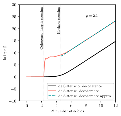
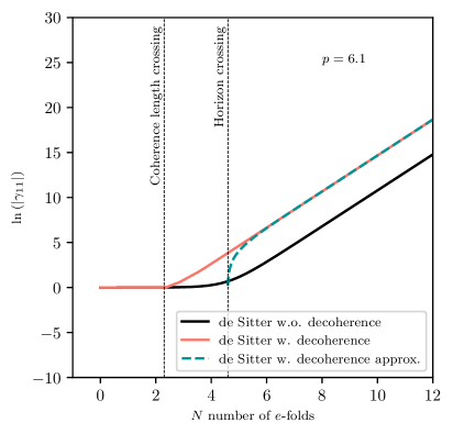
Figure 8: $\ln\left(|\gamma_{11}|\right)$ with (pink) and without (black) decoherence for the de Sitter case. The approximated version (green dashed) is obtained using the first order approximations (5.11). The first vertical dashed line shows the time when the mode $\bm{k}$ starts to decohere $\ell_{E}a/k=1$, the second the time when the mode $\bm{k}$ exits the Hubble radius. The parameters are $\ell_{E}H=0.1$, $x_{\star}=1$, $p=2.1$ (left) or $p=6.1$ (right), and $k_{\Gamma}/k=10$.

The next step consists in evaluating $\gamma_{12}$. Instead of using Eq. (4.16) and performing a similar calculation as above, one can use the transport equations (4.10), (4.11) and (4.12). This leads to

$$\gamma_{12}=\frac{1}{2k}\frac{{\mathrm{d}}}{{\mathrm{d}}\eta}\left(v_{\bm{k}}v_{\bm{k}}^{*}\right)+\left(\frac{k_{\Gamma}}{k}\right)^{2}\int_{-\infty}^{\eta}\left(\frac{a}{a_{*}}\right)^{p-3}\mathrm{H}\left(1-\frac{k\ell_{E}}{a}\right)\frac{\partial}{\partial\eta}{\rm Im}^{2}\left[v_{\bm{k}}(\eta)v_{\bm{k}}^{*}(\eta^{\prime})\right]{\mathrm{d}}\eta^{\prime}.$$ (D.8)

Instead of ${\rm Im}^{2}\left[v_{\bm{k}}(\eta)v_{\bm{k}}^{*}(\eta^{\prime})\right]$ in the integrand, as was the case for $\gamma_{11}$, we now have the derivative of it. Explicitly, written in terms of the variables $x$ and $x^{\prime}$, it can be expressed as

$$\frac{\partial}{\partial\eta}{\rm Im}^{2}\left[v_{\bm{k}}(\eta)v_{\bm{k}}^{*}(\eta^{\prime})\right] =\frac{k}{x^{3}x^{\prime 2}}(1+x^{\prime 2})-\frac{i}{2x^{3}x^{\prime 2}}e^{-2ix}e^{2ix^{\prime}}k(-i+x)\left[-1+x(-i+x)\right]$$

$$\times(i+x^{\prime})^{2}+\frac{i}{2x^{3}x^{\prime 2}}e^{2ix}e^{-2ix^{\prime}}k(i+x)\left[-1+x(i+x)\right](-i+x^{\prime})^{2}.$$ (D.9)

As a consequence, $\gamma_{12}$ takes the following form

$$\gamma_{12}=\frac{1}{2k}\frac{{\mathrm{d}}}{{\mathrm{d}}\eta}\left[v_{\bm{k}}(\eta)v_{\bm{k}}^{*}(\eta)\right]-2\left(\frac{k_{\Gamma}}{k}\right)^{2}\left[I_{12}^{(1)}+I_{12}^{(2)}+I_{12}^{(3)}\right],$$ (D.10)

with

$$I_{12}^{(1)} =\frac{1}{2}\frac{x_{*}^{p-3}}{x^{3}}\int_{1/(\ell_{E}H)}^{x}x^{\prime 1-p}(1+x^{\prime 2}){\mathrm{d}}x^{\prime},$$ (D.11)

$$I_{12}^{(2)} =-\frac{ix_{*}^{p-3}}{4x^{3}}e^{-2ix}(-i+x)\left[x(-i+x)-1\right]\int_{1/(\ell_{E}H)}^{x}e^{2ix^{\prime}}x^{\prime 1-p}(i+x^{\prime})^{2}{\mathrm{d}}x^{\prime},$$ (D.12)

$$I_{12}^{(3)} =\frac{ix_{*}^{p-3}}{4x^{3}}e^{2ix}(i+x)\left[x(i+x)-1\right]\int_{1/(\ell_{E}H)}^{x}e^{-2ix^{\prime}}x^{\prime 1-p}(-i+x^{\prime})^{2}{\mathrm{d}}x^{\prime}.$$ (D.13)

These integrals are very similar to those appearing in the expression (D.1) of $\gamma_{11}$ and they can be computed with the same techniques. We obtain

$$I_{12}^{(1)} =\frac{1}{2}\frac{x_{*}^{p-3}}{x^{3}}\left[\frac{x^{2-p}}{2-p}+\frac{x^{4-p}}{4-p}-\frac{(\ell_{E}H)^{p-2}}{2-p}-\frac{(\ell_{E}H)^{p-4}}{4-p}\right],$$ (D.14)

$$I_{12}^{(2)} =-\frac{ix_{*}^{p-3}}{4x^{3}}e^{-2ix}(-i+x)\left[x(-i+x)-1\right]\left(-A_{1-p}+2iA_{2-p}+A_{3-p}\right),$$ (D.15)

and $I_{12}^{(3)}=I_{12}^{(2)}{}^{*}$. In Fig. 9, we have plotted $\gamma_{12}$ with the same parameter values as in Fig. 8, namely $\ell_{E}=0.1$, $x_{*}=0.1$, $p=2.1$ and $k_{\Gamma}/k=10$.

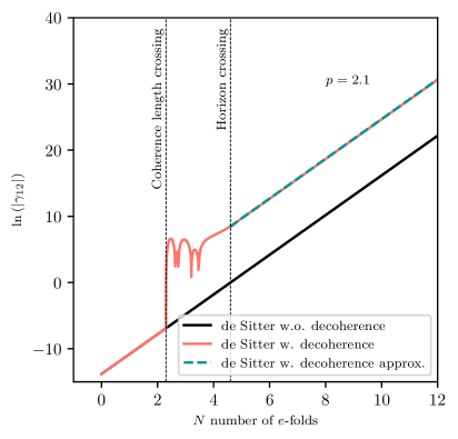
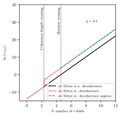
Figure 9: $\ln\left(|\gamma_{12}|\right)$ with (pink) and without (black) decoherence for the de Sitter case. The approximated version (green dashed) is obtained using the first order approximations (5.12). The first vertical dashed line shows the time when the mode $\bm{k}$ starts to decohere $\ell_{E}a/k=1$, the second the time when the mode $\bm{k}$ exits the Hubble radius. The parameters are $\ell_{E}H=0.1$, $x_{\star}=1$, $p=2.1$ (left) or $p=6.1$ (right), and $k_{\Gamma}/k=10$.

Finally, the component $\gamma_{22}$ remains to be evaluated. As done above for the component $\gamma_{12}$, one can use the transport equations to calculate $\gamma_{22}$ from the expression of $\gamma_{11}$. This leads to the following expression

$$\gamma_{22}= \frac{1}{2k^{2}}\frac{{\mathrm{d}}^{2}}{{\mathrm{d}}\eta^{2}}\left(v_{\bm{k}}v_{\bm{k}}^{*}\right)+\frac{1}{k}\left(\frac{k_{\Gamma}}{k}\right)^{2}\int_{-\infty}^{\eta}\left(\frac{a}{a_{*}}\right)^{p-3}\mathrm{H}\left(1-\frac{k\ell_{E}}{a}\right)\frac{\partial^{2}}{\partial\eta^{2}}{\rm Im}^{2}\left[v_{\bm{k}}(\eta)v_{\bm{k}}^{*}(\eta^{\prime})\right]{\mathrm{d}}\eta^{\prime}$$

$$+\frac{\omega^{2}}{k^{2}}\gamma_{11}.$$ (D.16)

As expected, the integrand in the above formula now contains the second derivative of ${\rm Im}^{2}\left[v_{\bm{k}}(\eta)v_{\bm{k}}^{*}(\eta^{\prime})\right]$. Concretely, this quantity can be written as

$$\frac{\partial^{2}}{\partial\eta^{2}}{\rm Im}^{2}\left[v_{\bm{k}}(\eta)v_{\bm{k}}^{*}(\eta^{\prime})\right] =\frac{3k^{2}}{x^{4}x^{\prime 2}}(1+x^{\prime 2})$$

$$+\frac{k^{2}}{2x^{4}x^{\prime 2}}e^{-2ix}e^{2ix^{\prime}}\left\{3+2x\left[3i+x(-3-2ix+x^{2})\right]\right\}(i+x^{\prime})^{2}$$

$$+\frac{k^{2}}{2x^{4}x^{\prime 2}}e^{2ix}e^{-2ix^{\prime}}\left\{3+2x\left[-3i+x(-3+2ix+x^{2})\right]\right\}(-i+x^{\prime})^{2}.$$ (D.17)

This leads to

$$\gamma_{22}= \frac{1}{2k^{2}}\frac{{\mathrm{d}}^{2}}{{\mathrm{d}}\eta^{2}}\left[v_{\bm{k}}(\eta)v_{\bm{k}}^{*}(\eta)\right]-2\left(\frac{k_{\Gamma}}{k}\right)^{2}\left[I_{22}^{(1)}+I_{22}^{(2)}+I_{22}^{(3)}\right]+\frac{\omega^{2}}{k^{2}}\gamma_{11}$$ (D.18)

$$= \frac{1}{2k^{2}}\frac{{\mathrm{d}}^{2}}{{\mathrm{d}}\eta^{2}}\left[v_{\bm{k}}(\eta)v_{\bm{k}}^{*}(\eta)\right]+\frac{\omega^{2}}{k^{2}}v_{\bm{k}}(\eta)v_{\bm{k}}^{*}(\eta)$$

$$-2\left(\frac{k_{\Gamma}}{k}\right)^{2}\left\{I_{22}^{(1)}+I_{22}^{(2)}+I_{22}^{(3)}++\frac{\omega^{2}}{k^{2}}\left[I_{11}^{(1)}+I_{11}^{(2)}+I_{11}^{(3)}\right]\right\},$$ (D.19)

with

$$I_{22}^{(1)} =\frac{3}{2}\frac{x_{*}^{p-3}}{x^{4}}\int_{1/(\ell_{E}H)}^{x}x^{\prime 1-p}(1+x^{\prime 2}){\mathrm{d}}x^{\prime},$$ (D.20)

$$I_{22}^{(2)} =\frac{x_{*}^{p-3}}{4x^{4}}e^{-2ix}\left\{3+2x\left[3i+x(-3-2ix+x^{2})\right]\right\}\int_{1/(\ell_{E}H)}^{x}e^{2ix^{\prime}}x^{\prime 1-p}(i+x^{\prime})^{2}{\mathrm{d}}x^{\prime},$$ (D.21)

$$I_{22}^{(3)} =\frac{x_{*}^{p-3}}{4x^{4}}e^{2ix}\left\{3+2x\left[-3i+x(-3+2ix+x^{2})\right]\right\}\int_{1/(\ell_{E}H)}^{x}e^{-2ix^{\prime}}x^{\prime 1-p}(-i+x^{\prime})^{2}{\mathrm{d}}x^{\prime}.$$ (D.22)

Again, the integrals $I_{22}^{(1)}$, $I_{22}^{(2)}$ and $I_{22}^{(3)}$ can be computed with the same tools used above. This leads to the following expressions

$$I_{22}^{(1)} =\frac{3}{2}\frac{x_{*}^{p-3}}{x^{4}}\left[\frac{x^{2-p}}{2-p}+\frac{x^{4-p}}{4-p}-\frac{(\ell_{E}H)^{p-2}}{2-p}-\frac{(\ell_{E}H)^{p-4}}{4-p}\right]$$ (D.23)

$$I_{22}^{(2)} =\frac{x_{*}^{p-3}}{4x^{4}}e^{-2ix}\left\{3+2x\left[3i+x(-3-2ix+x^{2})\right]\right\}\left(-A_{1-p}+2iA_{2-p}+A_{3-p}\right),$$ (D.24)

and $I_{22}^{(3)}=I_{22}^{(2)}{}^{*}$. The quantity $\gamma_{22}$ is represented in Fig. 10 for the same values of the parameters as above, that is to say $\ell_{E}H=0.1$, $x_{*}=1$, $p=2.1$, and $k_{\Gamma}/k=10$.

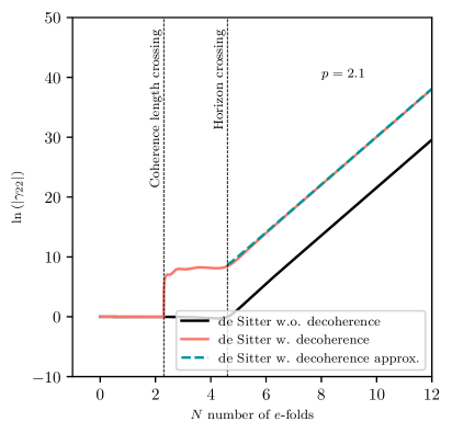
Figure 10: $\ln\left(|\gamma_{22}|\right)$ with (pink) and without (black) decoherence for the de Sitter case. The approximated version (green dashed) is obtained using the first order approximations (5.13). The first vertical dashed line shows the time when the mode $\bm{k}$ starts to decohere $\ell_{E}a/k=1$, the second the time when the mode $\bm{k}$ exits the Hubble radius. The parameters are $\ell_{E}H=0.1$, $x_{\star}=1$, $p=2.1$ (left) or $p=6.1$ (right), and $k_{\Gamma}/k=10$.

D.2 Approximations

The above results allow one to fully study the time evolution of the system, since they give exact and explicit expressions for the elements of the covariance matrix. However, the corresponding formulas are not particularly insightful and it is therefore useful to approximate them and to extract the leading behaviours of $\gamma_{11}$, $\gamma_{12}$ and $\gamma_{22}$ in the late time, i.e. super-Hubble, limit. This is the goal of this sub-section.

Let us start with the first component, $\gamma_{11}$. We write the function $A_{\alpha}$ in terms of its real and imaginary parts, $A_{\alpha}=A_{\alpha}^{\mathrm{R}}+iA_{\alpha}^{\mathrm{I}}$. Then, it follows that

$$I_{11}^{(2)}+I_{11}^{(3)} =\frac{x_{*}^{p-3}}{2x^{2}}\bigl{[}(x^{2}-1)\left(A_{1-p}^{\mathrm{R}}-A_{3-p}^{\mathrm{R}}+2A_{2-p}^{\mathrm{I}}\right)$$

$$+2x\left(A_{1-p}^{\mathrm{I}}-A_{3-p}^{\mathrm{I}}-2A_{2-p}^{\mathrm{R}}\right)\bigr{]}\cos(2x)$$

$$+\frac{x_{*}^{p-3}}{2x^{2}}\biggl{[}(x^{2}-1)\left(A_{1-p}^{\mathrm{I}}-A_{3-p}^{\mathrm{I}}-2A_{2-p}^{\mathrm{R}}\right)$$

$$-2x\left(A_{1-p}^{\mathrm{R}}-A_{3-p}^{\mathrm{R}}+2A_{2-p}^{\mathrm{I}}\right)\biggr{]}\sin(2x).$$ (D.25)

Since $I_{11}^{(3)}=I_{11}^{(2)}{}^{*}$, the quantity $I_{11}^{(2)}+I_{11}^{(3)}$ must be real and one can check that it is indeed the case. Then, upon Taylor expanding the real and imaginary parts of the function $A_{\alpha}$, defined in Eq. (D.7), around $x=0$, one obtains

$$A_{\alpha}^{\mathrm{R}} \simeq{\cal A}_{\alpha}^{\mathrm{R}}(\ell_{E}H)+x^{1+\alpha}\Biggl{[}\frac{1}{\alpha+1}-\frac{2x^{2}}{3+\alpha}+\frac{2x^{4}}{3(5+\alpha)}-\frac{4x^{6}}{45(7+\alpha)}$$

$$+\frac{2x^{8}}{315(9+\alpha)}-\frac{4x^{10}}{14175(11+\alpha)}+\frac{4x^{12}}{467775(13+\alpha)}-\frac{8x^{14}}{42567525(15+\alpha)}$$

$$+\frac{2x^{16}}{638512875(17+\alpha)}-\frac{4x^{18}}{97692469875(19+\alpha)}+\cdots\Biggr{]},$$ (D.26)

where

$${\cal A}_{\alpha}^{\mathrm{R}}(\ell_{E}H) =2^{-1-\alpha}\Gamma(1+\alpha)\sin\left(\frac{\pi\alpha}{2}\right)-i\,2^{-2-\alpha}\biggl{[}e^{-i\pi\alpha/2}\Gamma\left(1+\alpha,\frac{2i}{\ell_{E}H}\right)$$

$$-e^{i\pi\alpha/2}\Gamma\left(1+\alpha,-\frac{2i}{\ell_{E}H}\right)\biggr{]}.$$ (D.27)

The same type of calculations lead to the following expression for the imaginary part

$$A_{\alpha}^{\mathrm{I}} \simeq{\cal A}_{\alpha}^{\mathrm{I}}(\ell_{E}H)+x^{2+\alpha}\Biggl{[}\frac{2}{2+\alpha}-\frac{4x^{2}}{3(4+\alpha)}+\frac{4x^{4}}{15(6+\alpha)}-\frac{8x^{6}}{315(8+\alpha)}$$

$$+\frac{4x^{8}}{2835(10+\alpha)}-\frac{8x^{10}}{155925(12+\alpha)}+\frac{8x^{12}}{6081075(14+\alpha)}-\frac{16x^{14}}{638512875(16+\alpha)}$$

$$+\frac{4x^{16}}{10854718875(18+\alpha)}-\frac{8x^{18}}{1856156927625(20+\alpha)}+\cdots\Biggr{]},$$ (D.28)

where

$${\cal A}_{\alpha}^{\mathrm{I}}(\ell_{E}H) =-2^{-1-\alpha}\Gamma(1+\alpha)\cos\left(\frac{\pi\alpha}{2}\right)+2^{-2-\alpha}\biggl{[}e^{-i\pi\alpha/2}\Gamma\left(1+\alpha,\frac{2i}{\ell_{E}H}\right)$$

$$+e^{i\pi\alpha/2}\Gamma\left(1+\alpha,-\frac{2i}{\ell_{E}H}\right)\biggr{]}.$$ (D.29)

The next step consists in using the above approximations for the real and imaginary parts of $A_{\alpha}$ in Eq. (D.2) which, together with the exact expressions of $I_{11}^{(1)}$ (which is already given in terms of power-laws) leads to an approximation for the term $I_{11}^{(1)}+I_{11}^{(2)}+I_{11}^{(3)}$. The corresponding expression reads

$$I_{11}^{(1)}+I_{11}^{(2)}+I_{11}^{(3)}\simeq \,x^{-p}\left[A_{11}x^{6}+{\cal O}\left(x^{8}\right)\right]+\frac{B_{11}}{x^{2}}+C_{11}+D_{11}x+E_{11}x^{3}+F_{11}x^{4}$$

$$+G_{11}x^{5}+H_{11}x^{6}+{\cal O}\left(x^{7}\right)\,,$$ (D.30)

where

$$A_{11} =-\frac{2x_{*}^{p-3}}{(p-8)(p-5)(p-2)}$$ (D.31)

$$B_{11} =\frac{x_{*}^{p-3}}{2}\left[\frac{(\ell_{E}H)^{p-4}}{p-4}+\frac{(\ell_{E}H)^{p-2}}{p-2}-{\cal A}_{1-p}^{\mathrm{R}}-2{\cal A}_{2-p}^{\mathrm{I}}+{\cal A}_{3-p}^{\mathrm{R}}\right],$$ (D.32)

$$C_{11} =B_{11},$$ (D.33)

$$D_{11} =\frac{x_{*}^{p-3}}{3}\left(-{\cal A}_{1-p}^{\mathrm{I}}+2{\cal A}_{2-p}^{\mathrm{R}}+{\cal A}_{3-p}^{\mathrm{I}}\right),$$ (D.34)

$$E_{11} =\frac{2}{5}D_{11},$$ (D.35)

$$F_{11} =\frac{x_{*}^{p-3}}{9}\left({\cal A}_{1-p}^{\mathrm{R}}+2{\cal A}_{2-p}^{\mathrm{I}}-{\cal A}_{3-p}^{\mathrm{R}}\right),$$ (D.36)

$$G_{11} =-\frac{6}{35}D_{11},\quad H_{11}=-\frac{1}{5}F_{11}.$$ (D.37)

We combine the above with Eq. (D.1) to obtain an approximation of $\gamma_{11}$ which can be expressed as

$$\gamma_{11}=\frac{1}{x^{2}}\left[1-2\left(\frac{k_{\Gamma}}{k}\right)^{2}B_{11}\right]+\mathcal{O}\left(x^{0}\right)-2\left(\frac{k_{\Gamma}}{k}\right)^{2}A_{11}x^{6-p}+{\cal O}\left(x^{8-p}\right)\,.$$ (D.38)

Which of the two terms in the expression dominates depends on the value of $p$. This asymptotic expression of $\gamma_{11}$ is represented by the green dashed line in Fig. 8. We see that it matches very well the exact result.

Let us now derive an approximation for the matrix element $\gamma_{12}$. Compared to what has been done above for $\gamma_{11}$, the calculation proceeds in a similar fashion. The expression of $I_{12}^{(1)}$ is already explicit, see Eq. (D.14). The two remaining terms, $I_{12}^{(2)}$ and $I_{12}^{(3)}$, have similar expressions in terms of the real and imaginary parts of $A_{\alpha}$ as $I_{11}^{(2)}$ and $I_{11}^{(3)}$. This leads to

$$I_{12}^{(2)}+I_{12}^{(3)} =\frac{x_{*}^{p-3}}{2x^{3}}\biggl{[}(1-2x^{2})\left(-A_{1-p}^{\mathrm{R}}-2A_{2-p}^{\mathrm{I}}+A_{3-p}^{\mathrm{R}}\right)$$

$$-x(2-x^{2})\left(-A_{1-p}^{\mathrm{I}}+2A_{2-p}^{\mathrm{R}}+A_{3-p}^{\mathrm{I}}\right)\biggr{]}\cos(2x)$$

$$+\frac{x_{*}^{p-3}}{2x^{3}}\biggl{[}(1-2x^{2})\left(-A_{1-p}^{\mathrm{I}}+2A_{2-p}^{\mathrm{R}}+A_{3-p}^{\mathrm{I}}\right)$$

$$+x(2-x^{2})\left(-A_{1-p}^{\mathrm{R}}-2A_{2-p}^{\mathrm{I}}+A_{3-p}^{\mathrm{R}}\right)\biggr{]}\sin(2x).$$ (D.39)

Using this result and expanding consistently the result, one obtains the following expression

$$I_{12}^{(1)}+I_{12}^{(2)}+I_{12}^{(3)} \simeq x^{-p}\left[A_{12}x^{5}+{\cal O}\left(x^{7}\right)\right]+\frac{B_{12}}{x^{3}}+C_{12}+D_{12}x^{2}+E_{12}x^{3}$$

$$+F_{12}x^{4}+G_{12}x^{5}+H_{12}x^{6}+{\cal O}\left(x^{7}\right),$$ (D.40)

with

$$A_{12}=-\frac{x_{*}^{p-3}(p-6)}{(p-8)(p-5)(p-2)},$$ (D.41)

and $B_{12}=B_{11}$, $C_{12}=-D_{11}/2$, $D_{12}=-3D_{11}/5$, $E_{12}=-2F_{11}$, $F_{12}=3D_{11}/7$, $G_{12}=3F_{11}/5$ and $H_{12}=-2D_{11}/27$. Using Eq. (D.10) we get

$$\gamma_{12}=\frac{1}{x^{3}}\left[1-2\left(\frac{k_{\Gamma}}{k}\right)^{2}B_{12}\right]+{\cal O}\left(x^{0}\right)-2\left(\frac{k_{\Gamma}}{k}\right)^{2}\left[A_{12}x^{5-p}+{\cal O}\left(x^{7-p}\right)\right]\,,$$ (D.42)

Again, which of the two terms dominates in the above equation depends on the value of $p$. The approximation (D.42) is represented in Fig. 9 and we notice that, in its domain of validity (namely, on large scales), it is very accurate.

Let us finally consider the matrix element $\gamma_{22}$. In order to establish its large scale expansion, the considerations presented before can be repeated once more. The term $I_{22}^{(1)}$ has already the adequate form, see Eq. (D.23). As a consequence, the only calculation that is needed is to express $I_{22}^{(2)}+I_{22}^{(3)}$ in terms of the real and imaginary parts of $A_{\alpha}$. One obtains

$$I_{22}^{(2)}+I_{22}^{(3)} =\frac{x_{*}^{p-3}}{2x^{4}}\biggl{[}(3-6x^{2}+2x^{4})\left(-A_{1-p}^{\mathrm{R}}-2A_{2-p}^{\mathrm{I}}+A_{3-p}^{\mathrm{R}}\right)$$

$$-(6x-4x^{3})\left(-A_{1-p}^{\mathrm{I}}+2A_{2-p}^{\mathrm{R}}+A_{3-p}^{\mathrm{I}}\right)\biggr{]}\cos(2x)$$

$$+\frac{x_{*}^{p-3}}{2x^{4}}\biggl{[}(3-6x^{2}+2x^{4})\left(-A_{1-p}^{\mathrm{I}}+2A_{2-p}^{\mathrm{R}}+A_{3-p}^{\mathrm{I}}\right)$$

$$+(6x-4x^{3})\left(-A_{1-p}^{\mathrm{R}}-2A_{2-p}^{\mathrm{I}}+A_{3-p}^{\mathrm{R}}\right)\biggr{]}\sin(2x).$$ (D.43)

The next step consists in inserting the expressions (D.2) and (D.2) of the real and imaginary parts of $A_{\alpha}$ in the above formula. This leads to the following equation for the correction

$$I_{22}^{(1)} +I_{22}^{(2)}+I_{22}^{(3)}+\frac{\omega^{2}}{k^{2}}\left[I_{11}^{(1)}+I_{11}^{(2)}+I_{11}^{(3)}\right]=x^{-p}\left[A_{22}x^{4}+{\cal O}\left(x^{6}\right)\right]+\frac{B_{22}}{x^{4}}+\frac{C_{22}}{x^{2}}$$

$$+\frac{D_{22}}{x}+E_{22}+F_{22}x+G_{22}x^{2}+H_{22}x^{3}+I_{22}x^{4}+J_{22}x^{5}+K_{22}x^{6}+{\cal O}\left(x^{7}\right)\,,$$ (D.44)

with

$$A_{22} =-\frac{[26+p(p-11)]x_{*}^{p-3}}{(p-8)(p-5)(p-2)},$$ (D.45)

and $B_{22}=B_{11}$, $C_{22}=-B_{11}$, $D_{22}=-2D_{11}$, $E_{22}=B_{11}$, $F_{22}=7D_{11}/5$, $G_{22}=4F_{11}$, $H_{22}=-34D_{11}/35$, $I_{22}=-8F_{11}/5$, $J_{22}=218D_{11}/945$ and $K_{22}=43F_{11}/175$. Finally, we obtain the following approximation for $\gamma_{22}$

$$\gamma_{22}(\eta) =\frac{1}{x^{4}}\left[1-2\left(\frac{k_{\Gamma}}{k}\right)^{2}B_{22}\right]+{\cal O}\left(\frac{1}{x^{2}}\right)-2\left(\frac{k_{\Gamma}}{k}\right)^{2}A_{22}x^{4-p}+{\cal O}\left(x^{6-p}\right)\,.$$ (D.46)

This approximation (D.46) is plotted in Fig. 10 and we notice that it fits very well the exact result. Summarising, we have obtained, for each component of the covariant matrix, precise and simple approximations valid on large scales.

An interesting feature of the above calculations is the relationships that exist between the coefficients of the expansions of $\gamma_{11}$, $\gamma_{12}$ and $\gamma_{22}$. This can be understood as follows. Combining Eqs. (4.10) and (4.12), one has

$$-\frac{\mathrm{d}\gamma_{22}}{\mathrm{d}x}=\frac{\omega^{2}}{k^{2}}\frac{\mathrm{d}\gamma_{11}}{\mathrm{d}x}+2\left(\frac{k_{\Gamma}}{k}\right)^{2}x_{*}^{p-3}x^{3-p}.$$ (D.47)

Then, one can insert Eqs. (D.38) and (D.46) in the above formula and this leads to

$$\frac{4}{x^{5}}- 2\left(\frac{k_{\Gamma}}{k}\right)^{2}\left[\frac{4B_{22}}{x^{5}}-(4-p)A_{22}x^{3-p}\right]=-\frac{2}{x^{3}}+\frac{4}{x^{5}}-2\left(\frac{k_{\Gamma}}{k}\right)^{2}\biggl{[}-\frac{2B_{11}}{x^{3}}$$

$$+(6-p)A_{11}x^{5-p}+\frac{4B_{11}}{x^{5}}-2(6-p)A_{11}x^{3-p}\biggr{]}+2\left(\frac{k_{\Gamma}}{k}\right)^{2}x_{*}^{p-3}x^{3-p}.$$ (D.48)

At this stage, one has to remember that the expressions used above are valid in the long time limit only. Therefore, the term $-2/x^{3}$ (first term on the right hand side) can be neglected compared to $4/x^{5}$ (second term in the right hand side) and, indeed, the equation is satisfied in the limit $k_{\Gamma}\rightarrow 0$. Applying the same reasoning for the terms proportional to $k_{\Gamma}^{2}$, one deduces that $B_{22}=B_{11}$, a relation already established before but whose origin is now understood, and

$$(4-p)A_{22}=2(6-p)A_{11}+x_{*}^{p-3}.$$ (D.49)

One checks that this equation is satisfied by $A_{11}$ and $A_{22}$ given in Eqs. (D.31) and (D.45). Of course, the above considerations are just an example illustrating the origin of the relationships between the coefficients. A systematic generalisation of these calculations, with more terms in the expansions, would allow us to derive all the relationships among the coefficients.

References

- [1] A.A. Starobinsky, Spectrum of relict gravitational radiation and the early state of the universe, JETP Lett. 30 (1979) 682.
- [2] V.F. Mukhanov and G.V. Chibisov, Quantum Fluctuations and a Nonsingular Universe, JETP Lett. 33 (1981) 532.
- [3] L.P. Grishchuk and Y.V. Sidorov, Squeezed quantum states of relic gravitons and primordial density fluctuations, Phys. Rev. D 42 (1990) 3413.
- [4] D. Polarski and A.A. Starobinsky, Semiclassicality and decoherence of cosmological perturbations, Class. Quant. Grav. 13 (1996) 377 [gr-qc/9504030].
- [5] J. Martin and V. Vennin, Quantum Discord of Cosmic Inflation: Can we Show that CMB Anisotropies are of Quantum-Mechanical Origin?, Phys. Rev. D 93 (2016) 023505 [1510.04038].
- [6] J.S. Bell, On the Einstein-Podolsky-Rosen paradox, Physics Physique Fizika 1 (1964) 195.
- [7] M. Brune, E. Hagley, J. Dreyer, X. Maitre, A. Maali, C. Wunderlich et al., Observing the Progressive Decoherence of the ’Meter’ in a Quantum Measurement, Phys. Rev. Lett. 77 (1996) 4887.
- [8] L. Henderson and V. Vedral, Classical, quantum and total correlations, 0105028.
- [9] H. Ollivier and W.H. Zurek, Quantum Discord: A Measure of the Quantumness of Correlations, Phys. Rev. Lett. 88 (2001) 017901.
- [10] A. Bera, T. Das, D. Sadhukhan, S. Singha Roy, A. Sen De and U. Sen, Quantum discord and its allies: a review of recent progress, Reports on Progress in Physics 81 (2018) 024001 [1703.10542].
- [11] A. Datta, A Condition for the Nullity of Quantum Discord, arXiv e-prints (2010) arXiv:1003.5256 [1003.5256].
- [12] W.H. Zurek, Pointer Basis of Quantum Apparatus: Into What Mixture Does the Wave Packet Collapse?, Phys. Rev. D 24 (1981) 1516.
- [13] W.H. Zurek, Environment induced superselection rules, Phys. Rev. D 26 (1982) 1862.
- [14] V.F. Mukhanov, H.A. Feldman and R.H. Brandenberger, Theory of cosmological perturbations. Part 1. Classical perturbations. Part 2. Quantum theory of perturbations. Part 3. Extensions, Phys. Rept. 215 (1992) 203.
- [15] C.P. Burgess, R. Holman and D. Hoover, Decoherence of inflationary primordial fluctuations, Phys.Rev. D77 (2008) 063534 [astro-ph/0601646].
- [16] D. Campo and R. Parentani, Decoherence and entropy of primordial fluctuations. i. formalism and interpretation, Phys. Rev. D 78 (2008) 065044.
- [17] S. Choudhury, S. Panda and R. Singh, Bell violation in the Sky, Eur. Phys. J. C 77 (2017) 60 [1607.00237].
- [18] T.J. Hollowood and J.I. McDonald, Decoherence, discord and the quantum master equation for cosmological perturbations, Phys. Rev. D 95 (2017) 103521 [1701.02235].
- [19] J. Martin and V. Vennin, Observational constraints on quantum decoherence during inflation, JCAP 05 (2018) 063 [1801.09949].
- [20] J. Martin and V. Vennin, Non Gaussianities from Quantum Decoherence during Inflation, JCAP 06 (2018) 037 [1805.05609].
- [21] J. Martin and V. Vennin, Real-space entanglement in the Cosmic Microwave Background, 2106.15100.
- [22] S.-Y. Lin, C.-H. Chou and B.L. Hu, Quantum entanglement and entropy in particle creation, Phys. Rev. D 81 (2010) 084018 [1001.4922].
- [23] J.-T. Hsiang and B.-L. Hu, Intrinsic Entropy of Squeezed Quantum Fields and Nonequilibrium Quantum Dynamics of Cosmological Perturbations, 2110.02757.
- [24] J. Grain and V. Vennin, Canonical transformations and squeezing formalism in cosmology, JCAP 02 (2020) 022 [1910.01916].
- [25] J. Martin and V. Vennin, Real-space entanglement of quantum fields, 2106.14575.
- [26] S. Robertson, F. Michel and R. Parentani, Assessing degrees of entanglement of phonon states in atomic Bose gases through the measurement of commuting observables, Phys. Rev. D 96 (2017) 045012 [1705.06648].
- [27] G. Adesso, S. Ragy and A.R. Lee, Continuous variable quantum information: Gaussian states and beyond, Open Systems & Information Dynamics 21 (2014) 1440001.
- [28] R. Simon, E.C.G. Sudarshan and N. Mukunda, Gaussian-wigner distributions in quantum mechanics and optics, Phys. Rev. A 36 (1987) 3868.
- [29] R. Simon, E. Sudarshan and N. Mukunda, Gaussian wigner distributions: A complete characterization, Physics Letters A 124 (1987) 223 .
- [30] W.B. Case, Wigner functions and weyl transforms for pedestrians, American Journal of Physics 76 (2008) 937 [https://doi.org/10.1119/1.2957889].
- [31] C. Cohen-Tannoudji, J. Dupont-Roc and G. Grunberg, Atom - Photon Interactions: Basic Process and Appilcations, Wiley-Interscience (1992).
- [32] M. Le Bellac, Quantum Physics, Cambridge University Press (2006).
- [33] P. Pearle, Simple Derivation of the Lindblad Equation, Eur. J. Phys. 805 (2012) [1204.2016].
- [34] R.d.J.N. Carlos Alexandre Brasil, Felipe Fernandes Fanchini, A simple derivation of the Lindblad equation, Rev. Bras. Ensino Fís. 35 (2012) [1110.2122].
- [35] G. Lindblad, On the Generators of Quantum Dynamical Semigroups, Commun. Math. Phys. 48 (1976) 119.
- [36] G. Kaplanek and C.P. Burgess, Hot Accelerated Qubits: Decoherence, Thermalization, Secular Growth and Reliable Late-time Predictions, JHEP 03 (2020) 008 [1912.12951].
- [37] A.O. Caldeira and A.J. Leggett, Influence of dissipation on quantum tunneling in macroscopic systems, Phys. Rev. Lett. 46 (1981) 211.
- [38] A.O. Caldeira and A.J. Leggett, Quantum tunneling in a dissipative system, Annals Phys. 149 (1983) 374.
- [39] A.O. Caldeira and A.J. Leggett, Path integral approach to quantum Brownian motion, Physica A 121 (1983) 587.
- [40] H. Kodama and M. Sasaki, Cosmological Perturbation Theory, Prog. Theor. Phys. Suppl. 78 (1984) 1.
- [41] Y.-R. Chen, H.-Y. Hsieh, J. Ning, H.-C. Wu, H.L. Chen, Y.-L. Chuang et al., Experimental Reconstruction of Wigner Distribution Currents in Quantum Phase Space, 2111.08285.
- [42] P. Giorda and M.G.A. Paris, Gaussian Quantum Discord, Phys. Rev. Lett. 105 (2010) 020503 [1003.3207].
- [43] J. Martin and V. Vennin, Bell inequalities for continuous-variable systems in generic squeezed states, Phys. Rev. A 93 (2016) 062117 [1605.02944].
- [44] J. Martin and V. Vennin, Leggett-Garg Inequalities for Squeezed States, Phys. Rev. A 94 (2016) 052135 [1611.01785].
- [45] J. Martin and V. Vennin, Obstructions to Bell CMB Experiments, Phys. Rev. D 96 (2017) 063501 [1706.05001].
- [46] K. Ando and V. Vennin, Bipartite temporal Bell inequalities for two-mode squeezed states, Phys. Rev. A 102 (2020) 052213 [2007.00458].
- [47] R. Simon, Peres-horodecki separability criterion for continuous variable systems, Phys. Rev. Lett. 84 (2000) 2726.
- [48] H. Goldstein, C. Poole and J. Safko, Classical Mechanics, Addison Wesley (2002).
- [49] T. Colas, J. Grain and V. Vennin, Four-mode squeezed states: two-field quantum systems and the symplectic group , 2104.14942.
- [50] A.S. Holevo and R.F. Werner, Evaluating capacities of Bosonic Gaussian channels, arXiv e-prints (1999) quant [quant-ph/9912067].
- [51] G. Adesso and A. Datta, Quantum versus Classical Correlations in Gaussian States, Phys. Rev. Lett. 105 (2010) 030501 [1003.4979].
- [52] H. Goldstein, C. Poole and J. Safko, Classical Mechanics, Addison Wesley (2002).
- [53] I.S. Gradshteyn and I.M. Ryzhik, Table of Integrals, Series, and Products, Academic Press, New York and London (1965).
- [54] M. Abramowitz and I.A. Stegun, Handbook of Mathematical Functions with Formulas, Graphs, and Mathematical Tables, Dover, New York City, ninth dover printing, tenth gpo printing ed. (1964).