Double saddle-point preconditioning for Krylov methods in the inexact sequential homotopy method

Abstract

We derive an extension of the sequential homotopy method that allows for the application of inexact solvers for the linear (double) saddle-point systems arising in the local semismooth Newton method for the homotopy subproblems. For the class of problems that exhibit (after suitable partitioning of the variables) a zero in the off-diagonal blocks of the Hessian of the Lagrangian, we propose and analyze an efficient, parallelizable, symmetric positive definite preconditioner based on a double Schur complement approach. For discretized optimal control problems with PDE constraints, this structure is often present with the canonical partitioning of the variables in states and controls. We conclude with numerical results for a badly conditioned and highly nonlinear benchmark optimization problem with elliptic partial differential equations and control bounds. The resulting method allows for the parallel solution of large 3D problems.

1 Introduction

We are interested in approximately solving large-scale optimization problems of the form

$$\min\phi({x})\text{ over }{x}\in C\text{ subject to }c({x})=0,$$ (1)

where the objective functional $\phi:X\to\mathbb{R}$ and the equality constraint $c:X\to Y$ are twice continuously differentiable and $X=\mathbb{R}^{n}$, $Y=\mathbb{R}^{m}$, equipped with inner products

$$\left({u},{v}\right)_{X}={u}^{T}M_{X}{v},\quad\left({u},{v}\right)_{Y}={u}^{T}M_{Y}{v},$$

for sparse symmetric positive definite matrices $M_{X}\in\mathbb{R}^{n\times n}$ and $M_{Y}\in\mathbb{R}^{m\times m}$. We model inequality constraints by the nonempty closed convex set

$$C=\{{x}\in\mathbb{R}^{n}\mid{x}^{\mathrm{l}}_{i}\leq{x}_{i}\leq{x}^{\mathrm{u}}_{i}\text{ for }i=1,\dotsc,n\}$$ (2)

with lower and upper variable bounds ${x}^{\mathrm{l}}<{x}^{\mathrm{u}}\in\overline{\mathbb{R}}^{n}$, whose entries may take on values of $\pm\infty$. Moreover, we assume that the constraint Jacobian $c^{\prime}(x)$, the objective Hessian $\nabla^{2}\phi(x)$, and all constraint Hessians $\nabla^{2}c_{i}(x)$, $i=1,\dotsc,m$, are sparse matrices.

A sequential homotopy method has recently been proposed [51] for the approximate solution of a Hilbert space generalization of (1), where the resulting linear saddle-point systems were numerically solved by direct methods based on sparse matrix decompositions. The aim of this article is to address the challenges that arise when the linear systems are solved only approximately by Krylov-subspace methods and to analyze and leverage novel preconditioners that exploit a multiple saddle-point structure, in particular double saddle-point form, which often arises in optimal control problems with partial differential equation (PDE) constraints [39, 58, 44]. We restrict the presentation here to finite but high-dimensional $X$ and $Y$ to stay focused on the linear algebra issues.

The design principle of the sequential homotopy method is staying in a neighborhood of a suitably defined flow, which can be interpreted as the result of an idealized method with infinitesimal stepsize. Flows of this kind were first used by Davidenko [10] and later extended by various researchers as the basis for a plethora of globalization methods [2, 11, 12, 33, 14, 7, 13, 49, 50, 6, 51], often with a focus on affine invariance principles and partly to infinite-dimensional problems. However, special care needs to be taken for most of these approaches when solving nonconvex optimization problems, as the Newton flow is attracted to saddle points and maxima. Here we extend the sequential homotopy method of [51], which solves a sequence of projected backward Euler steps on a projected gradient/antigradient flow, to allow for inexact linear system solutions and hence the use of Krylov-subspace methods. Salient properties of the sequential homotopy method are that the difficulties of nonconvexity and constraint degeneracy are handled on the nonlinear level by an implicit regularization similar to regularized/stabilized Sequential Quadratic Programming (see, e.g., [62, 27, 22, 20, 21]). If semismooth Newton methods (see, e.g., [40, 52, 9, 34, 59, 31, 32, 35, 30, 29]) are applied, the resulting methods can handle the inequality constraints in an active-set fashion. Active-set methods are of high interest, especially when a sequence of related problems needs to be solved, because warm-starts that reuse the solution from a previously solved problem can be easily accomplished. For approaches based on interior-point methods (see, e.g., [25]), efficient warm-starting is still an unsolved issue.

We propose and analyze new preconditioners for the resulting linear system at each iteration of the sequential homotopy method. Preconditioning PDE-constrained optimization problems has been a subject of considerable interest of late (see, e.g., [55, 53, 63, 47, 45, 46, 48, 43]), however relatively few such methods have made use of the double saddle-point structure. We refer the reader to recent, related work [39, 58, 44, 8]. We provide theoretical results on preconditioners for double saddle-point systems and, having arranged the linear systems obtained from the active-set approach to this form, we present efficient and flexible approximations to be applied within a Krylov-subspace solver. Having explained each approximation step, we demonstrate the performance of a block-diagonal (and also a block-triangular) preconditioner on a highly nonlinear benchmark optimization problem, and present some results on potential parallelizability.

This paper is structured as follows. Section 2 states the sequential homotopy method and its Krylov-subspace active-set interpretation. In Section 3, we propose the use of an inexact semismooth Newton corrector in the sequential homotopy method and discuss the active-set-dependent linear systems which we need to solve. Section 4 gives results on preconditioners for double saddle-point matrices, which is the form of these systems, and Section 5 contains details of our implementation and approximations in our preconditioners. Section 6 presents a range of numerical results.

2 Sequential homotopy method

We briefly recapitulate the sequential homotopy method proposed in [51]. Let

$$L^{\rho}(x,y):=\phi(x)+\frac{\rho}{2}c(x)^{T}M_{Y}^{-1}c(x)+y^{T}c(x)$$

denote the augmented Lagrangian with some sufficiently large $\rho\geq 0$.

The sequential homotopy method solves a sequence of subproblems that differ in $(\hat{x},\hat{y})\in C\times Y$ and a homotopy parameter $\Delta t>0$:

$$x-P_{C}\left(\hat{x}-\Delta t\nabla_{x}L^{\rho}(x,y)\right) =0,$$ (3)

$$y-\phantom{P_{C}\,}\left(\hat{y}+\Delta t\nabla_{y}L^{\rho}(x,y)\right) =0,$$

for the unknowns $(x,y)\in X\times Y$, where $P_{C}$ is the (in general nonsmooth) projection onto $C$. By [51, Thm. 4], we know that for sufficiently small $\Delta t>0$, (3) admits a unique solution provided that a Lipschitz condition on $\nabla L^{\rho}$ holds. For $\Delta t=0$, the solution to (3) is $(x,y)=(\hat{x},\hat{y})$. If a continuation of solutions $(x(\Delta t),y(\Delta t))$ to (3) exists for $\Delta t\to\infty$, then $x(\Delta t),y(\Delta t)$ tends to a critical point of the original problem (1). If the solution $(x(\Delta t),y(\Delta t))$ cannot be continued (or if we decide not to follow it) further than some finite $\Delta t^{\ast}>0$, we can update the reference point $(\hat{x},\hat{y})=(x(\Delta t^{\ast}),y(\Delta t^{\ast}))$ and recommence the next homotopy leg (hence the name sequential homotopy method).

Local semismooth Newton methods are ideal candidates to solve (3) (see [51]), because the solution is close to $(\hat{x},\hat{y})$ if $\Delta t>0$ is sufficiently small. From this vantage point, our investigation of inexact semismooth Newton methods for (3) provides a class of active-set methods that are based on Krylov-subspace methods, which work particularly well in combination with suitable preconditioners such as those provided in Section 4.

3 Homotopy method with inexact semismooth Newton corrector

Although a local semismooth Newton method could in principle be applied to (3) directly, we prefer to equivalently reformulate (3) to avoid numerical issues for large $\Delta t$ and to obtain symmetric linearized systems (up to nonsymmetric active set modifications). This approach is possible for general symmetric positive definite $M_{X}$, but we prefer to restrict the discussion to the important special case where $M_{X}$ is a diagonal matrix, which reduces the notational and computational burden significantly. We elaborate on this restriction in the context of finite element (FE) discretizations in Sec. 4. In the case of diagonal $M_{X}$, the projection $P_{C}(v)=\operatorname*{arg\,min}_{x\in C}\left\lVert x-v\right\rVert_{X}$ can be represented by entrywise clipping via

$$P_{C}(v)_{i}:=\max\left(x^{\mathrm{l}}_{i},\min\left(v_{i},x^{\mathrm{u}}_{i}\right)\right)\quad\text{for }i=1,\dotsc,n.$$ (4)

To achieve a better scaling for large $\Delta t$, we premultiply the rows of equation system (3) by $\lambda M_{X}$ and $-\lambda M_{Y}$, where $\lambda=1/\Delta t$, which leads to the equivalent system

$$F(x,y;\hat{x},\hat{y},\lambda)=\begin{pmatrix}F_{1}(x,y;\hat{x},\hat{y},\lambda)\\ F_{2}(x,y;\hat{x},\hat{y},\lambda)\end{pmatrix}:=\begin{pmatrix}\lambda M_{X}\left(x-P_{C}(\hat{x}-\Delta t\nabla_{x}L^{\rho}(x,y))\right)\\ -\lambda M_{Y}(y-\hat{y})+M_{Y}\nabla_{y}L^{\rho}(x,y)\end{pmatrix}=0.$$ (5)

It is apparent that $F(\cdot,\cdot\,;\hat{x},\hat{y},\lambda)$ is Lipschitz continuous and piecewise continuously differentiable and, hence, semismooth [56, 59]. In each iteration of a semismooth Newton method for solving (5), we first need to evaluate $F$ at the current iterate $(x,y)$. Denoting the diagonal entries of $M_{X}$ by $d_{i}>0$, $i=1,\dotsc,n$ and using that the gradient is the Riesz representation of the derivative, the argument $v$ of $P_{C}$ in (5) consists of the entries

$$v_{i}=\hat{x}_{i}-\frac{\Delta t}{d_{i}}\frac{\mathrm{d}}{\mathrm{d}x_{i}}L^{\rho}(x,y).$$

We then identify the lower and upper active sets by comparing $v$ with $x^{\mathrm{l}}$ and $x^{\mathrm{u}}$ as

$$\mathbb{A}^{\mathrm{l}} :=\left\{i\mid x^{\mathrm{l}}_{i}\geq v_{i}\right\}=\left\{i\mid\tfrac{\mathrm{d}}{\mathrm{d}x_{i}}L^{\rho}(x,y)\geq\lambda d_{i}(\hat{x}_{i}-x^{\mathrm{l}}_{i})\right\},$$ (6)

$$\mathbb{A}^{\mathrm{u}} :=\left\{i\mid x^{\mathrm{u}}_{i}\leq v_{i}\right\}=\left\{i\mid\tfrac{\mathrm{d}}{\mathrm{d}x_{i}}L^{\rho}(x,y)\leq\lambda d_{i}(\hat{x}_{i}-x^{\mathrm{u}}_{i})\right\}.$$

This leads to the representations

$$F_{1}(x,y;\hat{x},\hat{y},\lambda)_{i} =\begin{cases}\lambda d_{i}(x_{i}-x^{\mathrm{l}}_{i})&\text{for }i\in\mathbb{A}^{\mathrm{l}},\\ \lambda d_{i}(x_{i}-x^{\mathrm{u}}_{i})&\text{for }i\in\mathbb{A}^{\mathrm{u}},\\ \lambda d_{i}(x_{i}-\hat{x}_{i})+\tfrac{\mathrm{d}}{\mathrm{d}x_{i}}L^{\rho}(x,y)&\text{otherwise},\end{cases}$$

$$F_{2}(x,y;\hat{x},\hat{y},\lambda) =-\lambda M_{Y}(y-\hat{y})+c(x).$$

An element of the set-valued generalized derivative $\partial F(x,y;\hat{x},\hat{y},\lambda)$ can then conveniently be constructed by substitution of the active rows $i\in\mathbb{A}:=\mathbb{A}^{\mathrm{l}}\cup\mathbb{A}^{\mathrm{u}}$ of the symmetric matrix

$$\lambda\mathop{\operator@font diag}\nolimits(M_{X},-M_{Y})+\nabla^{2}L^{\rho}(x,y)=\begin{pmatrix}\lambda M_{X}+H^{\rho}&G^{T}\\ G&-\lambda M_{Y}\end{pmatrix}$$

by rows consisting entirely of zeros except for diagonal entries of $\lambda d_{i}$, $i=1,\dotsc,n$. Here, we have used the abbreviations $G=c^{\prime}(x)$, $H=\nabla^{2}L^{0}(x,y+\rho M_{Y}^{-1}c(x))$ and write that $H^{\rho}=\nabla^{2}_{xx}L^{\rho}(x,y)=H+\rho G^{T}M_{Y}^{-1}G$.

We can then multiply all active rows $i\in\mathbb{A}$ and all active entries of the residual $-F(x,y;\hat{x},\hat{y},\lambda)$ by $\Delta t/d_{i}$, and permute all active rows and columns to the upper left of the linear system to arrive at

$$\begin{pmatrix}\mathrm{I}_{\left\lvert\mathbb{A}\right\rvert}&0&0\\ \mathrm{I}_{\overline{\mathbb{A}}}^{T}\left[\lambda M_{X}+H^{\rho}\right]\mathrm{I}_{\mathbb{A}}&\lambda\tilde{M}_{X}+\tilde{H}^{\rho}&\tilde{G}^{T}\\ G\mathrm{I}_{\mathbb{A}}&\tilde{G}&-\lambda M_{Y}\end{pmatrix}\begin{pmatrix}\Delta x_{\mathbb{A}}\\ \Delta x_{\overline{\mathbb{A}}}\\ \Delta y\end{pmatrix}=-\begin{pmatrix}b_{0}\\ b_{1}\\ b_{2}\end{pmatrix},$$ (7)

with $\overline{\mathbb{A}}=\{1,\dotsc,n\}\setminus\mathbb{A}$, $\mathrm{I}_{\mathbb{A}}$ a rectangular matrix consisting of the columns $i\in\mathbb{A}$ of $\mathrm{I}_{n}$ (likewise for $\mathrm{I}_{\overline{\mathbb{A}}}$), $\tilde{M}_{X}=\mathrm{I}_{\overline{\mathbb{A}}}^{T}M_{X}\mathrm{I}_{\overline{\mathbb{A}}}$, $\tilde{H}^{\rho}=\mathrm{I}_{\overline{\mathbb{A}}}^{T}H^{\rho}\mathrm{I}_{\overline{\mathbb{A}}}$, and $\tilde{G}=G\mathrm{I}_{\overline{\mathbb{A}}}$.

The same nonlinear transformation as in [51, Sec. 5.1] can be used to avoid forming the dense matrix $G^{T}M_{Y}^{-1}G$ in $H^{\rho}$ so that we only need to solve the sparse system

$$\begin{pmatrix}\mathrm{I}_{\left\lvert\mathbb{A}\right\rvert}&0&0\\ \mathrm{I}_{\overline{\mathbb{A}}}^{T}\left[\lambda M_{X}+H\right]\mathrm{I}_{\mathbb{A}}&\lambda\tilde{M}_{X}+\tilde{H}&\tilde{G}^{T}\\ G\mathrm{I}_{\mathbb{A}}&\tilde{G}&-\frac{\lambda}{1+\rho\lambda}M_{Y}\end{pmatrix}\begin{pmatrix}\Delta x_{\mathbb{A}}\\ \Delta x_{\overline{\mathbb{A}}}\\ \Delta\tilde{y}\end{pmatrix}=-\begin{pmatrix}b_{0}\\ b_{1}\\ \tilde{b}_{2}\end{pmatrix},$$ (8)

where $\tilde{b}_{2}=\frac{1}{1+\rho\lambda}b_{2}$ and $\tilde{H}=\mathrm{I}_{\overline{\mathbb{A}}}^{T}H\mathrm{I}_{\overline{\mathbb{A}}}$. The solution $\Delta y$ of (7) can then be recovered from $\Delta\tilde{y}$ via $\Delta y=\frac{1}{1+\rho\lambda}(\Delta\tilde{y}+\rho M_{Y}^{-1}b_{2}).$

Data: $z_{0}=(x_{0},y_{0})\in C\times Y$, $0<\theta_{\mathrm{ref}}<\theta_{\mathrm{max}}<1$, $0<\lambda_{\mathrm{min}}\leq\lambda_{\mathrm{term}}$, $0<\lambda_{\mathrm{red}}<1<\lambda_{\mathrm{inc}}$, $K_{P},K_{I}\geq 0$, $\mathrm{tol}>0$

1 Initialize $x=x_{0}$, $y=y_{0}$, $\lambda=1$, $I_{\mathrm{PI}}=0$

2 for $k=0,1,\dotsc$ do

3       Update reference $\hat{x}=x$, $\hat{y}=y$, set accept $=$ false

       — Preparations for semismooth Newton corrector steps —

4       Compute $b_{2}=c(x)$, Riesz rep. $r=M_{Y}^{-1}b_{2}$, and $b_{1}=\frac{\mathrm{d}}{\mathrm{d}x}L^{0}(x,y+\rho r)^{T}$

5       Compute $\mathcal{H}=\nabla^{2}L^{0}(x,y+\rho r)$

6       while not accept do

             — Semismooth Newton corrector step —

7             Set $\mathbb{A}^{\mathrm{l}}=\{i\mid(b_{1})_{i}\geq\lambda d_{i}(\hat{x}_{i}-x^{\mathrm{l}}_{i})\}$, $\mathbb{A}^{\mathrm{u}}=\{i\mid(b_{1})_{i}\leq\lambda d_{i}(\hat{x}_{i}-x^{\mathrm{u}}_{i})\}$

8             Set $(\tilde{b}_{1})_{i}=x_{i}-x^{\mathrm{l/u}}_{i}$ for $i\in\mathbb{A}$ and $(\tilde{b}_{1})_{i}=(b_{1})_{i}$ for $i\in\overline{\mathbb{A}}$

9             Scale $\tilde{b}_{2}=\frac{1}{1+\rho\lambda}b_{2}$

10             Compose $\hat{\mathcal{A}}=\mathop{\operator@font diag}\nolimits\bigl{(}\lambda M_{X},-\frac{\lambda}{1+\rho\lambda}M_{Y}\bigr{)}+\mathcal{H}$

11             Copy $\tilde{\mathcal{A}}=\hat{\mathcal{A}}$ and override rows $i\in\mathbb{A}$ of $\tilde{\mathcal{A}}$ with $e_{i}^{T}$

12             Solve $\displaystyle\tilde{\mathcal{A}}\begin{pmatrix}\Delta x\\ \Delta\tilde{y}\end{pmatrix}=-\begin{pmatrix}\tilde{b}_{1}\\ \tilde{b}_{2}\end{pmatrix}$ approximately

13             Recover $\Delta y=\frac{1}{1+\rho\lambda}(\Delta\tilde{y}+\rho r)$

14             Project step $x^{+}=P_{C}(x+\Delta x)$ and set $y^{+}=y+\Delta y$

             — Simplified semismooth Newton corrector step —

15             Compute $b_{2}^{+}=\lambda M_{Y}(\hat{y}-y^{+})+c(x^{+})$, $r^{+}=M_{Y}^{-1}b_{2}^{+}$, $b_{1}^{+}=\frac{\mathrm{d}}{\mathrm{d}x}L^{0}(x^{+},y^{+}+\rho r^{+})^{T}$

16             Set $\mathbb{A}^{\mathrm{l}}=\{i\mid(b^{+}_{1})_{i}\geq\lambda d_{i}(\hat{x}_{i}-x^{\mathrm{l}}_{i})\}$, $\mathbb{A}^{\mathrm{u}}=\{i\mid(b^{+}_{1})_{i}\leq\lambda d_{i}(\hat{x}_{i}-x^{\mathrm{u}}_{i})\}$

17             Set $(\tilde{b}^{+}_{1})_{i}=x^{+}_{i}-x^{\mathrm{l/u}}_{i}$ for $i\in\mathbb{A}$, $(\tilde{b}^{+}_{1})_{i}=\lambda d_{i}(x^{+}_{i}-\hat{x}_{i})+(b^{+}_{1})_{i}$ for $i\in\overline{\mathbb{A}}$

18             Scale $\tilde{b}_{2}^{+}=\frac{1}{1+\rho\lambda}b_{2}^{+}$

19             Copy $\tilde{\mathcal{A}}=\hat{\mathcal{A}}$ and override rows $i\in\mathbb{A}^{+}$ of $\tilde{\mathcal{A}}$ with $e_{i}^{T}$

20             Solve $\displaystyle\tilde{\mathcal{A}}\begin{pmatrix}\Delta x^{+}\\ \Delta\tilde{y}^{+}\end{pmatrix}=-\begin{pmatrix}\tilde{b}_{1}^{+}\\ \tilde{b}_{2}^{+}\end{pmatrix}$ approximately

21             Recover $\Delta y^{+}=\frac{1}{1+\rho\lambda}(\Delta\tilde{y}^{+}+\rho r^{+})$

22             Project step $x^{++}=P_{C}(x^{+}+\Delta x^{+})$ and set $y^{++}=y^{+}+\Delta y^{+}$

             — Stepsize adjustment —

23             Set $\theta=\left(\frac{\left\lVert\smash[t]{x^{++}-x^{+}}\right\rVert_{X}^{2}+\left\lVert\smash[t]{y^{++}-y^{+}}\right\rVert_{Y}^{2}}{\left\lVert\smash[t]{x^{+}-x}\right\rVert_{Y}^{2}+\left\lVert\smash[t]{y^{+}-y}\right\rVert_{Y}^{2}}\right)^{1/2}$

24             if $\theta\leq\theta_{\mathrm{max}}$ then (monotonicity test successful)

25                   Set accept $=$ true, $x=x^{++}$, $y=y^{++}$

26                   if $\left\lVert x-\hat{x}\right\rVert_{X}^{2}+\left\lVert y-\hat{y}\right\rVert_{Y}^{2}\leq\mathrm{tol}^{2}$ and $\lambda\leq\lambda_{\mathrm{term}}$ then return $(x,y)$

27                   if $\theta>0$ then (stepsize PI controller)

28                         Set $e=\log(\theta_{\mathrm{ref}})-\log(\theta)$

29                         Set $\lambda=\max(\lambda\exp(-K_{P}e-K_{I}I_{\mathrm{PI}}),\lambda_{\mathrm{min}})$, update $I_{\mathrm{PI}}=I_{\mathrm{PI}}+e$

30                        

31                  else

32                         Reduce $\lambda=\max(\lambda\cdot\lambda_{\mathrm{red}},\lambda_{\mathrm{min}})$

33                        

34                  

35            else

36                   Increase $\lambda=\lambda\cdot\lambda_{\mathrm{inc}}$

37                   if $I_{\mathrm{PI}}>0$ then set $I_{\mathrm{PI}}=0$

38                  

39            

40      

Algorithm 1 Inexact sequential homotopy method

When a symmetric Krylov-subspace method is started with an initial guess that solves the first block row of (8) exactly, then the generated Krylov subspace will only depend on the symmetric 2-by-2 block in the lower right, and symmetric Krylov-subspace methods can safely be used. Hence, preconditioners are only required for the symmetric part of (8).

We provide a pseudocode description of the inexact sequential homotopy method in Alg. 1. The algorithm employs only one inexact semismooth Newton step plus one simplified (i.e., without updating the system matrix except for active set changes) semismooth Newton step, and then simultaneously updates the reference point $(\hat{x},\hat{y})$ and $\lambda$ in $F$. Additionally, the permutation of the active rows and columns to the top-left block of the system is not performed explicitly.

As a practical implementation, we use [51, Alg. 1], with the modification that the linear systems are solved approximately. The choice of the relative termination tolerance $\kappa\geq 0$ for the preconditioned residual norm of the Krylov-subspace method to approximately solve the linear systems involving $\tilde{\mathcal{A}}$ is a delicate issue here. The choice should effect less accurate and thus less expensive linear system solves when far away from the solution. In contrast to the setting in, e.g., [9], there are more involved restrictions on $\kappa$, because we are shooting at a moving target inside the homotopy method. Unfortunately, these restrictions are, at least so far, hard to quantify. Qualitatively, the size of the tolerance $\kappa$ must be balanced with the size of $\lambda$. Ultimately, we would like to have a small $\lambda$ to progress fast on the nonlinear level, but this would necessitate small $\kappa$ to stay within the (moving) region of local convergence. Hence, we propose the affine-linear-plus-saturation heuristic

$$\kappa=P_{[\kappa_{\mathrm{min}},\kappa_{\mathrm{max}}]}\left(\kappa_{\mathrm{max}}+(\kappa_{\mathrm{min}}-\kappa_{\mathrm{max}})\tfrac{\lambda-\lambda^{r}_{0}}{\lambda^{r}_{1}-\lambda^{r}_{0}}\right).$$

We employ this heuristic in the numerical experiments with the values set to $\kappa_{\mathrm{min}}=10^{-7},$ $\kappa_{\mathrm{max}}=10^{-3},$ $\lambda^{r}_{0}=1,$ $\lambda^{r}_{1}=10^{-7}.$ We further enforce $\lambda\geq\lambda_{\mathrm{min}}=10^{-7}$ in the adaptive stepsize control.

The numerical criterion for evaluating whether we keep inside the region of local convergence is the same increment monotonicity test as described in [51, Alg. 1], which also serves as the basis for the adaptive stepsize control. The stepsize proportional-integral (PI) controller constants are the same as in [51, Alg. 1].

4 Preconditioned iterative methods for double saddle-point systems

To derive efficient preconditioners, it is important to exploit additional problem structure. We take interest here in a special property of discretizations of a large class of PDE-constrained optimal control problems:

$$\min{} \frac{1}{2}\left\lVert u-u_{\mathrm{d}}\right\rVert^{2}_{V}+\frac{\gamma}{2}\left\lVert q-q_{\mathrm{d}}\right\rVert^{2}_{Q}$$ (9)

over $$(q,u)\in C_{Q}\times U,$$

s.t. $$c((u,q))=c((u,0))+c_{q}((0,0))q=0,$$

for which the matrix $H$ is of block-diagonal form, because the control and state variables are separated in the objective function and the control enters the (possibly nonlinear) state equation only affine linearly. We assume that the discretized space $X=Q\times U$ comprises discretized controls $q\in C_{Q}\subset Q$ and (unconstrained) discretized states $u\in C_{U}=U$ with a tracking term, while $y\in Y$ are the adjoint variables. We can model control bounds in $C_{Q}$, which is of the form (2).

The inner product matrix $M_{X}=\mathop{\operator@font diag}\nolimits(M_{Q},M_{U})$ is a block-diagonal matrix, which typically consists of a mass matrix $M_{Q}$ for the controls and a stiffness matrix $M_{U}$ for the states. The inner product matrix $M_{Y}$ is typically also a stiffness matrix. There are, however, good reasons to use only the diagonal of a mass matrix for $M_{Q}$ (mass lumping): spectral equivalence [61] leads to an equivalent norm with mesh-independent equivalence constants and, just like the pointwise formula for projections in $L^{2}$, the projector $P_{C}$ turns into an entrywise projection, which can be cheaply computed via (4).

Following the obvious extension of variable naming above, a symmetric permutation of (8) leads to

$$\begin{pmatrix}\mathrm{I}_{\left\lvert\mathbb{A}\right\rvert}&0&0&0\\ \ast&\lambda\tilde{M}_{Q}+\tilde{H}_{Q}&\tilde{G}_{Q}^{T}&0\\ \ast&\tilde{G}_{Q}&-\frac{\lambda}{1+\rho\lambda}M_{Y}&G_{U}\\ \ast&0&G_{U}^{T}&\lambda M_{U}+H_{U}\end{pmatrix}\begin{pmatrix}\Delta{q}_{\mathbb{A}}\\ \Delta{q}_{\overline{\mathbb{A}}}\\ \Delta\tilde{{y}}\\ \Delta{u}\end{pmatrix}=-\begin{pmatrix}{b}_{0}\\ {b}_{1,q}\\ \frac{1}{1+\rho\lambda}{b}_{2}\\ {b}_{1,u}\end{pmatrix}.$$ (10)

We remark here that the regularization parameter $\gamma$ only enters in the $\tilde{H}_{Q}$ block.

In this section we provide some theory of preconditioning matrices of the form

$$\ \mathcal{A}=\left(\begin{array}[]{ccc}A_{1}&B_{1}^{T}&0\\ B_{1}&-A_{2}&B_{2}^{T}\\ 0&B_{2}&A_{3}\\ \end{array}\right),$$ (11)

which are frequently referred to as double saddle-point systems. This is important, as the systems we are required to solve in this paper are of the form (11). Specifically, after (trivially) eliminating the first block-row in (10), we obtain a system of the form (11) from the lower right 3-by-3 blocks of (10). It is important that the proposed preconditioners are robust with respect to the augmented Lagrangian coefficient $\rho>0$ and the proximity parameter $\lambda$, which may typically vary between $10^{-12}$ and $10^{1}$.

We highlight that there has been much previous work on preconditioners for double saddle-point systems, see for example [19, 39, 1, 58]. In particular, [58] provides a comprehensive description of eigenvalues of preconditioned double saddle-point systems on the continuous level (i.e., by the operators involved). What follows in this section is an analysis for double saddle-point systems, inspired by the logic of the proof given in [39, Thm. 4].

For our forthcoming analysis we will make use of the following result, which concerns eigenvalues for generalized saddle-point systems preconditioned by a block-diagonal matrix. The bounds described below can be found elsewhere in the literature: for instance, see [3, Cor. 1], [57, Lem. 2.2], [42, Thm. 4].

Theorem 1.

Let

$$\ \mathcal{A}_{2}=\left(\begin{array}[]{cc}A_{1}&B^{T}\\ B&-A_{2}\\ \end{array}\right),\quad\quad\mathcal{P}_{2}=\left(\begin{array}[]{cc}A_{1}&0\\ 0&S_{1}\\ \end{array}\right),$$

where $A_{1}$, $S_{1}=A_{2}+BA_{1}^{-1}B^{T}$ are assumed to be symmetric positive definite, and $A_{2}$ is assumed to be symmetric positive semi-definite. Then all eigenvalues of $\mathcal{P}_{2}^{-1}\mathcal{A}_{2}$ satisfy $\mu\left(\mathcal{P}_{2}^{-1}\mathcal{A}_{2}\right)\in\left[-1,\frac{1}{2}(1-\sqrt{5})\right]\cup\left[1,\frac{1}{2}(1+\sqrt{5})\right].$

We now analyze a block-diagonal preconditioner for matrix systems of the form (11), in the simplified setting that $A_{3}=0$, using the logic of [39, Thm. 4].

Theorem 2.

Let

$$\ \mathcal{A}_{0}=\left(\begin{array}[]{ccc}A_{1}&B_{1}^{T}&0\\ B_{1}&-A_{2}&B_{2}^{T}\\ 0&B_{2}&0\\ \end{array}\right),\quad\quad\mathcal{P}_{D}=\left(\begin{array}[]{ccc}A_{1}&0&0\\ 0&S_{1}&0\\ 0&0&S_{2}\\ \end{array}\right),$$

where $A_{1}$, $S_{1}=A_{2}+B_{1}A_{1}^{-1}B_{1}^{T}$, $S_{2}=B_{2}S_{1}^{-1}B_{2}^{T}$ are assumed to be symmetric positive definite, and $A_{2}$ is assumed to be symmetric positive semi-definite. Then all eigenvalues of $\mathcal{P}_{D}^{-1}\mathcal{A}_{0}$ satisfy:

$$\ \mu\left(\mathcal{P}_{D}^{-1}\mathcal{A}_{0}\right)\in{} \left[-\frac{1}{2}(1+\sqrt{5}),2\hskip 1.49994pt\emph{cos}\left(\frac{5\pi}{7}\right)\right]\cup\left[-1,\frac{1}{2}(1-\sqrt{5})\right]$$

$$\quad\quad\cup\left[2\hskip 1.49994pt\emph{cos}\left(\frac{3\pi}{7}\right),\frac{1}{2}(\sqrt{5}-1)\right]\cup\left[1,2\hskip 1.49994pt\emph{cos}\left(\frac{\pi}{7}\right)\right],$$

which to $3$ decimal places are $[-1.618,-1.247]\cup[-1,-0.618]\cup[0.445,0.618]\cup[1,1.802]$.

Proof.

Examining the associated eigenproblem

$$\ \left(\begin{array}[]{ccc}A_{1}&B_{1}^{T}&0\\ B_{1}&-A_{2}&B_{2}^{T}\\ 0&B_{2}&0\\ \end{array}\right)\left(\begin{array}[]{c}x_{1}\\ x_{2}\\ x_{3}\\ \end{array}\right)=\mu\left(\begin{array}[]{ccc}A_{1}&0&0\\ 0&S_{1}&0\\ 0&0&S_{2}\\ \end{array}\right)\left(\begin{array}[]{c}x_{1}\\ x_{2}\\ x_{3}\\ \end{array}\right),$$

we obtain that

$$\ A_{1}x_{1}+B_{1}^{T}x_{2}={} \mu{}A_{1}x_{1},$$ (12a)

$$\ B_{1}x_{1}-A_{2}x_{2}+B_{2}^{T}x_{3}={} \mu{}S_{1}x_{2},$$ (12b)

$$\ B_{2}x_{2}={} \mu{}S_{2}x_{3}.$$ (12c)

We now prove the result by contradiction, that is we assume there exists an eigenvalue outside the stated intervals. From (12a), we see that

$$\ \alpha A_{1}x_{1}+B_{1}^{T}x_{2}=0\quad\Rightarrow\quad\alpha x_{1}=-A_{1}^{-1}B_{1}^{T}x_{2},$$ (13)

where $\alpha=1-\mu\neq 0$ by assumption. Substituting (13) into (12b) tells us that

$$\ 0={} \alpha\left[B_{1}x_{1}-(1+\mu)A_{2}x_{2}+B_{2}^{T}x_{3}-\mu{}B_{1}A_{1}^{-1}B_{1}^{T}x_{2}\right]$$

$$\ ={} -B_{1}A_{1}^{-1}B_{1}^{T}x_{2}-\alpha(1+\mu)A_{2}x_{2}+\alpha B_{2}^{T}x_{3}-\mu\alpha B_{1}A_{1}^{-1}B_{1}^{T}x_{2}$$

$$\ ={} -[\beta B_{1}A_{1}^{-1}B_{1}^{T}+\delta A_{2}]x_{2}+\alpha B_{2}^{T}x_{3},$$ (14)

where $\beta=1+\mu\alpha=1+\mu-\mu^{2}\neq 0$, $\delta=\alpha(1+\mu)=1-\mu^{2}\neq 0$ by assumption. Now, for the cases $\mu\in(-\infty,-1)$, $\mu\in(\frac{1}{2}(1-\sqrt{5}),1)$, and $\mu\in(\frac{1}{2}(1+\sqrt{5}),+\infty)$, $\beta$ and $\delta$ have the same signs (negative, positive, and negative, respectively), so $\beta B_{1}A_{1}^{-1}B_{1}^{T}+\delta A_{2}$ is a definite (and hence invertible) matrix. Thus, in these cases, (14) tells us that

$$\ x_{2}=\alpha[\beta B_{1}A_{1}^{-1}B_{1}^{T}+\delta A_{2}]^{-1}B_{2}^{T}x_{3},$$

which we may then substitute into (12c) to yield that

$$\ 0=\alpha B_{2}[\beta B_{1}A_{1}^{-1}B_{1}^{T}+\delta A_{2}]^{-1}B_{2}^{T}x_{3}-\mu{}B_{2}[B_{1}A_{1}^{-1}B_{1}^{T}+A_{2}]^{-1}B_{2}^{T}x_{3}.$$ (15)

We now highlight that $\mu\neq 0$; otherwise (15) would read that

$$\ 0=B_{2}[B_{1}A_{1}^{-1}B_{1}^{T}+A_{2}]^{-1}B_{2}^{T}x_{3}=S_{2}x_{3}\quad\Rightarrow\quad x_{3}=0,$$

which means that

$$\ \left(\begin{array}[]{cc}A_{1}&B_{1}^{T}\\ B_{1}&-A_{2}\\ \end{array}\right)\left(\begin{array}[]{c}x_{1}\\ x_{2}\\ \end{array}\right)=\mu\left(\begin{array}[]{cc}A_{1}&0\\ 0&S_{1}\\ \end{array}\right)\left(\begin{array}[]{c}x_{1}\\ x_{2}\\ \end{array}\right),$$

holds (along with $B_{2}x_{2}=0$). Applying Thm. 1 then gives that $\mu\in[-1,\frac{1}{2}(1-\sqrt{5})]\cup[1,\frac{1}{2}(1+\sqrt{5})]$, yielding a contradiction. Using that $\mu\neq 0$, as well as that $\alpha\neq 0$ by assumption, we may divide (15) by $\alpha\mu$ to obtain that

$$\ 0={} B_{2}[\mu\beta B_{1}A_{1}^{-1}B_{1}^{T}+\mu\delta A_{2}]^{-1}B_{2}^{T}x_{3}-B_{2}[\alpha B_{1}A_{1}^{-1}B_{1}^{T}+\alpha A_{2}]^{-1}B_{2}^{T}x_{3}$$

$$\ ={} B_{2}[\zeta B_{1}A_{1}^{-1}B_{1}^{T}+\eta A_{2}]^{-1}B_{2}^{T}x_{3}-B_{2}[\alpha B_{1}A_{1}^{-1}B_{1}^{T}+\alpha A_{2}]^{-1}B_{2}^{T}x_{3},$$

where $\zeta=\mu\beta=\mu+\mu^{2}-\mu^{3}$ and $\eta=\mu\delta=\mu-\mu^{3}$. As the situation $x_{3}=0$ reduces the problem to that of Thm. 1, where $\mu$ is contained within a subset of the intervals claimed here, we may reduce the analysis to the case $x_{3}\neq 0$ and write

$$\ 0=x_{3}^{T}B_{2}\left([\zeta B_{1}A_{1}^{-1}B_{1}^{T}+\eta A_{2}]^{-1}-[\alpha B_{1}A_{1}^{-1}B_{1}^{T}+\alpha A_{2}]^{-1}\right)B_{2}^{T}x_{3}=:x_{3}^{T}\Psi x_{3},$$ (16)

with both $B_{1}A_{1}^{-1}B_{1}^{T}$ and $A_{2}$ symmetric positive semi-definite. We now consider different cases (we have already excluded the possibility that $\mu=0$):

• $\mu\in(-\infty,-\frac{1}{2}(1+\sqrt{5})):$ Here $\alpha,\zeta,\eta>0$, such that $\zeta>\alpha$, $\eta>\alpha$. Hence $\zeta B_{1}A_{1}^{-1}B_{1}^{T}+\eta A_{2}\succ\alpha B_{1}A_{1}^{-1}B_{1}^{T}+\alpha A_{2}$ (meaning $[\zeta B_{1}A_{1}^{-1}B_{1}^{T}+\eta A_{2}]-[\alpha B_{1}A_{1}^{-1}B_{1}^{T}+\alpha A_{2}]$ is positive definite), and $\Psi$ is negative definite. This yields a contradiction with (16), so there is no $\mu\in(-\infty,-\frac{1}{2}(1+\sqrt{5}))$.

• $\mu\in(2\hskip 1.49994pt\text{cos}(\frac{5\pi}{7}),-1):$ Here $\alpha,\zeta,\eta>0$, such that $\zeta<\alpha$, $\eta<\alpha$. Hence $\zeta B_{1}A_{1}^{-1}B_{1}^{T}+\eta A_{2}\prec\alpha B_{1}A_{1}^{-1}B_{1}^{T}+\alpha A_{2}$ (meaning $[\zeta B_{1}A_{1}^{-1}B_{1}^{T}+\eta A_{2}]-[\alpha B_{1}A_{1}^{-1}B_{1}^{T}+\alpha A_{2}]$ is negative definite), and $\Psi$ is positive definite. Similarly to above, this yields a contradiction.

• $\mu\in(\frac{1}{2}(1-\sqrt{5}),0):$ Here, $\alpha>0$, $\zeta,\eta<0$, so $[\zeta B_{1}A_{1}^{-1}B_{1}^{T}+\eta A_{2}]^{-1}$ is negative definite and $[\alpha B_{1}A_{1}^{-1}B_{1}^{T}+\alpha A_{2}]^{-1}$ is positive definite. Therefore $\Psi$ is negative definite, yielding a contradiction.

• $\mu\in(0,2\hskip 1.49994pt\text{cos}(\frac{3\pi}{7})):$ Here $\alpha,\zeta,\eta>0$, such that $\zeta<\alpha$, $\eta<\alpha$. Hence $\zeta B_{1}A_{1}^{-1}B_{1}^{T}+\eta A_{2}\prec\alpha B_{1}A_{1}^{-1}B_{1}^{T}+\alpha A_{2}$, and $\Psi$ is positive definite, yielding a contradiction.

• $\mu\in(\frac{1}{2}(\sqrt{5}-1),1):$ Here $\alpha,\zeta,\eta>0$, such that $\zeta>\alpha$, $\eta>\alpha$. Hence $\zeta B_{1}A_{1}^{-1}B_{1}^{T}+\eta A_{2}\succ\alpha B_{1}A_{1}^{-1}B_{1}^{T}+\alpha A_{2}$, and $\Psi$ is negative definite, yielding a contradiction.

• $\mu\in(2\hskip 1.49994pt\text{cos}(\frac{\pi}{7}),+\infty):$ Here $\alpha,\zeta,\eta<0$, such that $\zeta<\alpha$, $\eta<\alpha$. Hence $\zeta B_{1}A_{1}^{-1}B_{1}^{T}+\eta A_{2}$ and $\alpha B_{1}A_{1}^{-1}B_{1}^{T}+\alpha A_{2}$ are both negative definite, such that $\zeta B_{1}A_{1}^{-1}B_{1}^{T}+\eta A_{2}\prec\alpha B_{1}A_{1}^{-1}B_{1}^{T}+\alpha A_{2}$. Therefore $[\zeta B_{1}A_{1}^{-1}B_{1}^{T}+\eta A_{2}]^{-1}\succ[\alpha B_{1}A_{1}^{-1}B_{1}^{T}+\alpha A_{2}]^{-1}$, and $\Psi$ is positive definite, yielding a contradiction.

The result is thus proved by contradiction. ∎

By applying the structure of the proof of Thm. 2, we may analyze the analogous block-diagonal preconditioner for (11), for the more general case that $A_{3}$ is symmetric positive semi-definite. The following retrieves the result shown in Thm. 3.3 of the recent paper [8], using a different structure of proof:

Theorem 3.

Let

$$\ \mathcal{P}_{D}=\left(\begin{array}[]{ccc}A_{1}&0&0\\ 0&S_{1}&0\\ 0&0&S_{2}\\ \end{array}\right),$$

with $\mathcal{A}$ as defined in (11), where $A_{1}$, $S_{1}=A_{2}+B_{1}A_{1}^{-1}B_{1}^{T}$, $S_{2}=A_{3}+B_{2}S_{1}^{-1}B_{2}^{T}$ are assumed to be symmetric positive definite, and $A_{2}$, $A_{3}$ are assumed to be symmetric positive semi-definite. Then all eigenvalues of $\mathcal{P}_{D}^{-1}\mathcal{A}$ satisfy:

$$\ \mu\left(\mathcal{P}_{D}^{-1}\mathcal{A}\right)\in\left[-\frac{1}{2}(1+\sqrt{5}),\frac{1}{2}(1-\sqrt{5})\right]\cup\left[2\hskip 1.49994pt\emph{cos}\left(\frac{3\pi}{7}\right),2\hskip 1.49994pt\emph{cos}\left(\frac{\pi}{7}\right)\right],$$

which to $3$ decimal places are $[-1.618,-0.618]\cup[0.445,1.802]$.

Remark 1.

The above result guarantees a fixed rate of convergence for preconditioned minres applied to systems of the form (11) with the properties stated. In [8], the authors also demonstrate the effect of approximating the blocks $A_{1}$, $S_{1}$, $S_{2}$ within the block-diagonal preconditioner, further highlighting the effectiveness of this strategy. We also highlight [8, Thm. 3.2], which analyzes the case $A_{2}=0$.

Along with block-diagonal preconditioners for (11), we may construct block-triangular preconditioners, stated and analyzed in the simple result below.

Theorem 4.

Let

$$\ \mathcal{P}_{L}=\left(\begin{array}[]{ccc}A_{1}&0&0\\ B_{1}&-S_{1}&0\\ 0&B_{2}&S_{2}\\ \end{array}\right),\quad\quad\mathcal{P}_{U}=\left(\begin{array}[]{ccc}A_{1}&B_{1}^{T}&0\\ 0&-S_{1}&B_{2}^{T}\\ 0&0&S_{2}\\ \end{array}\right),$$

with $\mathcal{A}$ as defined in (11), where $A_{1}$, $S_{1}=A_{2}+B_{1}A_{1}^{-1}B_{1}^{T}$, $S_{2}=A_{3}+B_{2}S_{1}^{-1}B_{2}^{T}$ are assumed to be invertible. Then all eigenvalues of $\mathcal{P}_{L}^{-1}\mathcal{A}$ and $\mathcal{P}_{U}^{-1}\mathcal{A}$ are equal to $1$.

Proof.

It may easily be verified that

$$\ \mathcal{P}_{L}^{-1}\mathcal{A}=\left(\begin{array}[]{ccc}\mathrm{I}&A_{1}^{-1}B_{1}^{T}&0\\ 0&\mathrm{I}&-S_{1}^{-1}B_{2}^{T}\\ 0&0&\mathrm{I}\\ \end{array}\right),\quad\quad\mathcal{A}\mathcal{P}_{U}^{-1}=\left(\begin{array}[]{ccc}\mathrm{I}&0&0\\ B_{1}A_{1}^{-1}&\mathrm{I}&0\\ 0&-B_{2}S_{1}^{-1}&\mathrm{I}\\ \end{array}\right),$$

which gives the result (with the result for $\mathcal{P}_{U}^{-1}\mathcal{A}$ inferred using similarity of this matrix and $\mathcal{A}\mathcal{P}_{U}^{-1}$). ∎

We note Thm. 4 makes no assumptions on the properties of $B_{2}$, or the positive definiteness of $A_{1}$, $S_{1}$, $S_{2}$, unlike Thms. 2 and 3. However, we note the limitations of Thm. 4: with a block-triangular preconditioner, diagonalizability of the preconditioned system is not given, and implementing this preconditioner requires a nonsymmetric iterative solver for which the eigenvalue distribution does not guarantee a fixed convergence rate.

It would also be possible to combine $P_{D}$, $P_{L}$, and $P_{U}$ into one symmetric positive definite preconditioner $P_{LDU}=P_{L}P_{D}^{-1}P_{U}$, an approach which we investigate separately in [44] for the more general case of multiple saddle-point systems of block-tridiagonal form. The parallel implementation of the preconditioner $P_{LDU}$ would also be possible with the same libraries that we use in Section 5, but at the expense of a more involved code. Because we focus on how to use indirect linear algebra methods inside the sequential homotopy method here, we restrict the numerical results to the use of the simpler preconditioners $P_{D}$ and $P_{L}$.

5 Implementation details

Among all problems of the form (9), we focus our attention in the remainder of this work to a family of nonlinear and possibly badly conditioned benchmark problems of the specific form (cf. [38, 51]):

$$\min{} \frac{1}{2}\int_{\Omega}\left\lvert u-u_{\mathrm{d}}\right\rvert^{2}+\frac{\gamma}{2}\int_{\Omega}\left\lvert q\right\rvert^{2}\quad \text{over }u\in H^{1}_{0}(\Omega),q\in L^{2}(\Omega)$$ (17)

s.t. $$\nabla\cdot\left(\left[a+b\left\lvert u\right\rvert^{2}\right]\nabla u\right)=q,\quad q_{\mathrm{l}}\leq q\leq q_{\mathrm{u}},$$

where $\Omega\subset\mathbb{R}^{d}$, $d=2,3$, is a bounded domain with Lipschitz boundary and $a,b,\gamma>0$ with control bounds $q_{\mathrm{l}},q_{\mathrm{u}}\in L^{s}(\Omega),s\in(2,\infty]$, and a tracking target function $u_{\mathrm{d}}\in L^{2}(\Omega)$. The difficulty of problem (17) can be tuned by the scalar parameters: smaller $\gamma$ and $a$ result in worse conditioning of the problem, while larger $b$ increases the nonlinearity. We caution that the interplay with the objective function is nontrivial: small values of $a$ in combination with large values of $b$ might lead to an optimal solution with small $|u|$ over $\Omega$, eventually resulting in less nonlinearity in the neighborhood of the optimal solution. We focus on $\gamma=10^{-6}$, $a=10^{-2}$, $b=10^{2}$, which was experienced as the most difficult instance in the numerical results in [51]. All remaining problem data was set to the values in [51].

After discretization of problem (17) with P1 finite elements, the application of Alg. 1 leads to a sequence of linear systems of the form (10). Eliminating the first block row, we arrive at a double saddle-point system of the form (11), with

$$A_{1}=\lambda\tilde{M}_{Q}+\tilde{H}_{Q},~{}~{}A_{2}=\frac{\lambda}{1+\rho\lambda}M_{Y},~{}~{}A_{3}=\lambda M_{U}+H_{U},~{}~{}B_{1}=\tilde{G}_{Q},~{}~{}B_{2}=G_{U}^{T},$$

$$S_{1}=\frac{\lambda}{1+\rho\lambda}M_{Y}+B_{1}(\lambda\tilde{M}_{Q}+\tilde{H}_{Q})^{-1}B_{1}^{T},\quad S_{2}=\lambda M_{U}+H_{U}+B_{2}S_{1}^{-1}B_{2}^{T}.$$

In order to efficiently apply the block preconditioners derived above, we need to approximately apply the inverse operations of $A_{1}$, $S_{1}$, $S_{2}$ to generic vectors, in a computationally efficient way. We note that an alternative strategy would be to apply preconditioners to a re-ordered system of (classical) saddle-point form (see [5, 41]), however for problems with the structures considered, the leading block of the matrix is likely to possess a more problematic structure, with implications on its preconditioned approximation as well as that of the resulting Schur complement.

Numerically, we compare a number of increasingly efficient preconditioner choices, which we elaborate on in more detail below:

1. Direct sparse decomposition of $\mathcal{A}$ without the use of Krylov-subspace solver, which can be considered as a preconditioner that leads to convergence in one step.

2. Basic Schur complement block-diagonal preconditioner with sparse decomposition of $A_{1}$, $\hat{S}_{1}$, $\hat{S}_{2}$, where $\hat{S}_{i}$ approximates $S_{i}$. For empty active sets, the approximations are exact.

3. Matching Schur complement block-diagonal preconditioner with sparse decomposition of $A_{1}$ and $\hat{S}_{1}$ in combination with a matching approach for $\hat{S}_{2}$ using sparse decompositions for the factors of the multiplicative approximation of $\hat{S}_{2}$.

4. AMG[$\hat{S}_{1}$] matching Schur complement block-diagonal preconditioner, which coincides with the matching Schur complement preconditioner, except using an Algebraic Multigrid (AMG) approximation for $\hat{S}_{1}^{-1}$ instead of a direct decomposition.

5. Decomposition-free Schur complement block-diagonal preconditioner with completely decomposition-free approximations of all Schur complements $A_{1}$, $S_{1}$, $S_{2}$ based on matching for $\hat{S}_{2}$. The preconditioner can be implemented using publicly-available, parallelizable preconditioners.

6. Block-triangular decomposition-free Schur complement preconditioner. In contrast to the previous preconditioners, this preconditioner must be used with a nonsymmetric solver such as gmres instead of minres because it is a block lower-triangular and not a symmetric preconditioner.

Each preconditioner in the list above serves as the baseline for the next in terms of number of nonlinear iterations, which are expected to grow from top to bottom, and the resulting computation time. We use FEniCS [15, 37] to discretize problem (17) with P1 finite elements and implemented all preconditioners in PETSc [17, 16, 4].

We do not provide further details for preconditioner choices 1 and 6 because the application of a direct sparse decomposition is straightforward and choice 6 is just the block-triangular version of the block-diagonal preconditioner of choice 5. In the remainder of this section, we elaborate on the choices 2–5.

5.1 Basic Schur complement preconditioner

We first recall the inner product matrices: the matrix $M_{Q}$ is the diagonal part of a FE mass matrix $M_{\mathrm{FE}}$. The matrices $M_{U}=M_{Y}$ are FE stiffness matrices. All of these can be easily assembled. Thus, $\tilde{M}_{Q}=\mathrm{I}_{\overline{\mathbb{A}}}^{T}M_{Q}\mathrm{I}_{\overline{\mathbb{A}}}$, $\tilde{H}_{Q}=\gamma\mathrm{I}_{\overline{\mathbb{A}}}^{T}M_{\mathrm{FE}}\mathrm{I}_{\overline{\mathbb{A}}}$, and $\tilde{G}_{Q}=M_{\mathrm{FE}}\mathrm{I}_{\overline{\mathbb{A}}}$. For the first Schur complement we obtain the explicit expressions

$$A_{1} =\lambda\tilde{M}_{Q}+\tilde{H}_{Q},\quad B_{1}=\tilde{G}_{Q},\quad A_{2}=\frac{\lambda}{1+\rho\lambda}M_{Y},$$

$$S_{1} =\frac{\lambda}{1+\rho\lambda}M_{Y}+M_{\mathrm{FE}}\mathrm{I}_{\overline{\mathbb{A}}}\left(\mathrm{I}_{\overline{\mathbb{A}}}^{T}(\lambda M_{Q}+\gamma M_{\mathrm{FE}})\mathrm{I}_{\overline{\mathbb{A}}}\right)^{-1}\mathrm{I}_{\overline{\mathbb{A}}}^{T}M_{\mathrm{FE}}.$$

We observe that for $\lambda=0$, the Schur complement $S_{1}$ has a nontrivial kernel spanned by $M_{\mathrm{FE}}^{-1}\mathrm{I}_{\mathbb{A}}$, while it is equal to $(1/\gamma)M_{\mathrm{FE}}\mathrm{I}_{\overline{\mathbb{A}}}$ on the orthogonal complement, which is spanned by $\mathrm{I}_{\overline{\mathbb{A}}}$. Based on these comments, we propose approximating $M_{\mathrm{FE}}$ on each occasion in $S_{1}$ by its diagonal $M_{Q}$ (independently of the active set $\mathbb{A}$) to derive a basic Schur complement preconditioner using the approximate Schur complement

$$\hat{S}_{1}=\frac{\lambda}{1+\rho\lambda}M_{Y}+\frac{1}{\lambda+\gamma}M_{Q}.$$

We remark that the stiffness term $M_{Y}$ dominates $\hat{S}_{1}$ for large $\lambda$ and for finer meshes with fixed (but possibly small) $\lambda$. We can use direct sparse decompositions of $A_{1}$ and $\hat{S}_{1}$ to compute the action of their inverses to high accuracy.

For the basic Schur complement preconditioner, we approximate $S_{2}$ using the approximate first Schur complement

$$\hat{S}_{2}=A_{2}+B_{2}\hat{S}_{1}^{-1}B_{2}^{T}.$$

Regarding the explicit structure of $\hat{S}_{2}$, we first note that $B_{2}$ is a nonsymmetric FE matrix for the linearized elliptic PDE operator with respect to the state. The direct assembly of $\hat{S}_{2}$ is prohibitive because $\hat{S}_{2}$ is a dense matrix. However, the action of $\hat{S}_{2}^{-1}$ can be computed by unrolling the Schur complement through a direct sparse decomposition of the sparse block matrix

$$\begin{pmatrix}\lambda M_{U}+H_{U}&B_{2}\\ B_{2}^{T}&-\hat{S}_{1}\end{pmatrix}.$$

We investigate this preconditioner purely to assess the quality of the Schur complement approach in general and as a baseline for the following Schur complement approximations. We discourage the use of the basic Schur complement preconditioner for the solution of (17).

5.2 Matching Schur complement preconditioner

We now address the approximation of the most delicate Schur complement $\hat{S}_{2}$ by a matching strategy, which has found considerable utility for PDE-constrained optimization problems [45, 47], including those with additional bound constraints [43, 46]. A key challenge is that inverses of matrix sums are much harder to apply than inverses of matrix products.

For the problem at hand, the second Schur complement has the explicit form

$$\hat{S}_{2} =\lambda M_{U}+H_{U}+B_{2}\hat{S}_{1}^{-1}B_{2}^{T}$$

$$=\lambda M_{U}+H_{U}+B_{2}\left[(1+\rho\lambda)^{-1}\lambda M_{Y}+(\lambda+\gamma)^{-1}M_{Q}\right]^{-1}B_{2}^{T}.$$

We now approximate $\hat{S}_{2}$ by a product $D\hat{S}_{1}^{-1}D^{T}$, where $D=\alpha_{1}M_{U}+\alpha_{2}M_{\mathrm{FE}}+B_{2}$ such that

$$\left(\alpha_{1}M_{U}+\alpha_{2}M_{\mathrm{FE}}\right)\hat{S}_{1}^{-1}\left(\alpha_{1}M_{U}+\alpha_{2}M_{\mathrm{FE}}\right)\approx\lambda{M}_{U}+{H}_{U},$$

and we wish to match the factors $\alpha_{1},\alpha_{2}>0$. As $H_{U}=M_{\mathrm{FE}}+N_{U}$, where $N_{U}$ contains nonlinear terms arising from the PDE operators, a computationally efficient choice is to neglect the effect of $N_{U}$, and match the terms in $M_{Y}$, $M_{\mathrm{FE}}$ separately. This heuristic strategy means we wish to select

$$\begin{array}[]{rcl}\left(\alpha_{1}M_{U}\right)\left[(1+\rho\lambda)^{-1}\lambda M_{Y}\right]^{-1}\left(\alpha_{1}M_{U}\right)=\lambda M_{U}&\Rightarrow&\alpha_{1}=\frac{\lambda}{\sqrt{1+\rho\lambda}},\\ \left(\alpha_{2}M_{\mathrm{FE}}\right)\left[(\lambda+\gamma)^{-1}M_{Q}\right]^{-1}\left(\alpha_{2}M_{\mathrm{FE}}\right)\approx M_{\mathrm{FE}}&\Rightarrow&\alpha_{2}=\frac{1}{\sqrt{\lambda+\gamma}},\end{array}$$

exploiting that $M_{U}=M_{Y}$ and $M_{Q}$ is the diagonal part of $M_{\mathrm{FE}}$. Note that we can readily assemble $D=\lambda(1+\rho\lambda)^{-1/2}M_{U}+(\lambda+\gamma)^{-1/2}M_{\mathrm{FE}}+B_{2}$ and use a direct sparse decomposition of $D$ to approximate $\hat{S}_{2}^{-1}$ with $\smash[t]{\hat{S}}_{2}^{-1}=D^{-T}\hat{S}_{1}D^{-1}$.

We highlight that the structure of certain terms within $\hat{S}_{2}$, and hence the effectiveness of the resulting approximations, are dependent on the problem structure considered. For instance, the matrix $B_{2}^{T}$ is dependent on the form of the (linearized) differential operator, and the regularization terms within the objective function will lead to rank-deficient matrices when (for instance) boundary control problems are considered; these structures will then arise within the preconditioner. We believe the complicated, highly nonlinear benchmark problem considered provides a challenging and realistic test for our proposed preconditioning strategy.

5.3 AMG[$\hat{S}_{1}$] matching Schur complement preconditioner

This approach extends the matching Schur complement preconditioner by using an AMG preconditioner to approximate $\hat{S}_{1}$. We use hypre/BoomerAMG [18, 28] with two sweeps of a V-cycle and one Jacobi iteration for each pre- and post-smoothing step.

5.4 Decomposition-free Schur complement preconditioner

This preconditioner further extends the AMG[$\hat{S}_{1}$] matching Schur complement preconditioner. The matrix $A_{1}$ is a FE mass matrix, so may be well approximated by its diagonal [61]. The use of a nested Conjugate Gradient (cg) solver for $A_{1}$ would require the use of a flexible outer Krylov-subspace solver such as flexible gmres [54] due to the nonlinearity of cg. Instead, we apply a fixed number of 15 linear Chebyshev semi-iterations (see [23, 24, 60]) on the diagonally-scaled $A_{1}$ with the optimal spectral bounds $[\frac{1}{2},2]$ (2D) and $[\frac{1}{2},\frac{5}{2}$] (3D) from [61], which are independent of the value of $\lambda$. Finally we also employ an AMG preconditioner for approximating the inverses of $D$ and $D^{T}$. We use hypre/BoomerAMG again with 4 V-cycle sweeps with two Jacobi sweeps for pre- and post-smoothing and a fixed relaxation weight of $0.7$. It is crucial to disable CF-relaxation for BoomerAMG to work correctly for application of the transposed preconditioner (see [36, p. 133]).

6 Numerical results

We solve problem (17) using the sequential homotopy method with the algorithmic parameters from [51], with the changes described above and the Schur complement approximations of Section 5, applying block-diagonally preconditioned minres and block-lower-triangularly preconditioned gmres. A maximum number of 200 Krylov method iterations is used. When there is no convergence within this number of iterations, it is an indication that the current matrix $\hat{S}_{2}$ might be indefinite. In this case, the nonlinear step is flagged as failed and the sequential homotopy method increases $\lambda$, which eventually renders $\hat{S}_{2}$ positive definite. For the simplified semismooth Newton step, we prescribe the same number of Krylov method iterations that were adaptively determined by the standard termination criterion in the preceeding semismooth Newton step. When a sequential homotopy iteration fails due to excess of Krylov method iterations or due to violation of the monotonicity test, we mark the iteration with a black cross in the following figures.

We perform numerical experiments for P1 FE discretizations on triangular meshes of the unit square/cube with a varying number $N$ of elements per side.

Fig. 1: Krylov solver iterations: minres with the basic Schur complement preconditioner. The case $N=640$ is omitted due to excessive runtime.

Fig. 2: Krylov solver iterations: minres with the matching Schur complement preconditioner.

Fig. 3: Krylov solver iterations: minres with the decomposition-free Schur complement preconditioner.

Fig. 4: Krylov solver iterations: gmres with the block-triangular decomposition-free Schur complement preconditioner.

Fig. 5: Krylov solver iterations: Comparison of different variants for $N=320$.

Fig. 6: Krylov solver iterations: Comparison of different variants for $N=640$.

Fig. 7: Comparison of wall clock time vs. iterations of different variants for $N=640$.

6.1 Preconditioner comparison for the 2D case

We start with the 2D instances. In Fig. 1 we see that for the basic Schur complement preconditioner the number of minres iterations per iteration of the sequential homotopy method stays moderately low (10–40 iterations) most of the time. Between iterations 20 and 30 as well as close to the solution, the number of iterations rises to about 60–80. This shows that the method saves numerical effort in the linear algebra part when being far away from the solution. The number of nonlinear iterations increases considerably when going from $N=160$ to $N=320$, which we attribute to the steep boundary layer of the optimal state, which is not faithfully resolved on meshes smaller than $N\leq 160$.

In Fig. 1–6, discarded iterations (due to $\theta>\theta_{\mathrm{max}}$ or Krylov-subspace methods failing to converge for a given linear system) are marked with an additional black $\times$.

Compared to Fig. 1, we see in Fig. 2 that the matching approach slightly increases the required number of minres iterations, while the number of nonlinear iterations stays roughly the same. In contrast to the basic Schur complement preconditioner (which takes more than 41 hours for $N=320$), also the case $N=640$ can be solved in under four hours now (cf. Fig. 7).

Using the AMG[$\hat{S}_{1}$] and decomposition-free Schur complement preconditioners result in qualitatively very similar behavior, so we just display the latter in Fig. 3. This exhibits the efficiency and robustness of the solver for a range of problem sizes.

Using the block-triangular version of the decomposition-free Schur complement preconditioner seems to deliver a more robust preconditioner with fewer fluctuations in the number of iterations (see Fig. 4).

We compare the number of required inner and outer iterations resulting from the different preconditioner variants on grids with fixed size in Fig. 5 ($N=320$) and Fig. 6 ($N=640$). We observe that the expected increase in the number of outer iterations for solving the linear subproblems inexactly with Krylov-subspace methods compared to direct decomposition approaches is moderate for $N=640$ (70 or better vs. 57). For $N=320$, some preconditioner choices perform better for the numerical challenges that start in outer iteration $k=33$, leading to fewer overall outer iterations. The differences are mostly due to the number of failed iterations (marked with $\times$), whenever the sequential homotopy method is forced to increase $\lambda$ to keep inside the region of local convergence for the nonlinear subproblems.

When it comes to runtime between all preconditioners, there is a clear benefit of using the decomposition-free Schur complement preconditioners, which are competitive with the use of direct linear algebra even for the 2D problem on a reasonably fine grid (see Fig. 7).

6.2 Parallelization for the 2D case

Fig. 8: Weak scaling results for 2D case using the block-diagonal decomposition free preconditioner and minres. We show the average wall clock times over the last 10 iterations on the finest grid level.

Number of processors	1	4	16	64
$N$	320	640	1,280	2,560
Degrees of freedom	309,123	1,232,643	4,922,883	19,676,163

Table 1: Correspondence of number of processors and discretization for the weak scaling experiment.

We report weak scaling results of the decomposition-free Schur complement preconditioner in Fig. 8 for up to 64 processors. The number of degrees of freedom for each run is provided in Tab. 1. In a case of perfect parallel scaling, all lines in Fig. 8 would be horizontal. There is a noticeable drop in parallel efficiency when the number of processors and degrees of freedom increase. However, this drop goes in conjunction with a drop in parallel efficiency also for the Riesz solver, which is simply AMG-preconditioned cg for the Poisson equation, whose parallel scaling can be considered state-of-the-art.

6.3 3D case

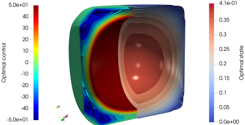
Fig. 9: Result for the 3D test case for $N=160$. The unit cube is cut in half in the $X/Y$ plane. On the left we see isosurfaces of the optimal control and on the right isosurfaces of the optimal state.

$N$	Degrees of freedom	Outer iter.	minres iter.	Wall clock time [min]
20	27,783	52	2693	1.67
40	206,763	39	1730	2.74
80	1,594,323	34	1186	12.06
160	12,519,843	35	760	63.20

Table 2: Statistics for the 3D test case on each discretization level. The computations were performed on 32 processors in parallel.

Fig. 10: Statistics for the iterations of the 3D test case on refined meshes. Failed iterations are indicated as missing dots in the first and third plot. The contraction $\theta$ is the quotient of the simplified step norm over the step norm.

Fig. 11: Slice through the X/Y plane of the absolute difference of the optimal state, control, and adjoint approximations on the two finest 3D meshes ($N=160$ minus $N=80$). The difference for the control is rather large close to the boundary of the active set (central gray region). The different magnitudes of the differences are partly due to the different numerical ranges (not shown), which are approximately $[0,0.41]$ (state), $[-50,50]$ (control), and $[-5\cdot 10^{-5},5\cdot 10^{-4}]$ (adjoint).

In Fig. 9 we show the optimal solution of the model problem (17) on the unit cube on a regular tetrahedral grid with $N=160$ element edges per edge of the unit cube and control bounds of $\pm 50$. Similar to the optimal solutions in 2D, the optimal controls and optimal states exhibit very steep slopes. The computations are carried out on a sequence of uniformly refined equidistant meshes for $N=20,40,80,160$. Starting with an initial guess of zero, we employ Alg. 1 with the block-diagonal decomposition-free preconditioner and the same tolerance of $\mathrm{tol}=10^{-5}$ as in the 2D case on each level, moving from the coarsest level to the finest while using the solution of the previous level as the initial guess on the next (finer) mesh. We have slightly reduced the augmentation parameter for the 3D test case from $\rho=10^{-1}$ to $\rho=10^{-3}$ to avoid occasionally failing iterations on the finer levels. In Tab. 2, we see that most CPU time is spent on the finest level and that comparably few minres iterations are required there. We depict further information about the iterations on the different levels in Fig. 10. From the contraction rates $\theta$ of the monotonicity test, we see that for the initial guesses on each level a rather large $\lambda$ is required to stay in the region of local convergence for the simplified semismooth Newton method, while later, fast local convergence with $\lambda=\lambda_{\mathrm{min}}$ can be achieved. Rather large increases in the step norms after refinement of the grid can be observed. We attribute these to the spatial resolution of the solution’s local features, such as steep slopes at the domain boundary and the boundary of the active set of the solution (cf. Fig. 9 and Fig. 11), which are very sensitive to the chosen finite element mesh. Altogether the proposed inexact sequential homotopy method with the suggested preconditioners can reliably and efficiently solve large-scale, highly nonlinear, badly conditioned problems.

7 Conclusion

We have extended a sequential homotopy method to allow the use of inexact solvers for the linearized subsystems. We provided analysis for symmetric positive definite, block-diagonal Schur complement preconditioners for double saddle-point systems, with a view to applying these to a prominent class of nonlinear PDE-constrained optimization problems. For a challenging model problem, we provided approximations of the Schur complements for the efficient and parallel application of approximated double saddle-point preconditioners. The implicit regularization feature of the sequential homotopy method was beneficial for the solution of the linearized subproblems with preconditioned minres and gmres. We provided numerical results for a hierarchy of Schur complement approximations, which shed light on the consequences of each approximation step on the way to the eventual fast, effective, and parallelizable, decomposition-free preconditioner. We provided a weak scaling analysis for the 2D case and efficiently solved a large 3D problem instance with 12 million degrees of freedom.

References

- [1] F. P. Ali Beik and M. Benzi. Iterative methods for double saddle point systems. SIAM J. Matrix Anal. Appl., 39(2):902–921, 2018.
- [2] K. J. Arrow, L. Hurwicz, and H. Uzawa. Studies in linear and non-linear programming. With contributions by H. B. Chenery, S. M. Johnson, S. Karlin, T. Marschak, R. M. Solow. Stanford Mathematical Studies in the Social Sciences, vol. II. Stanford University Press, Stanford, CA, 1958.
- [3] O. Axelsson and M. Neytcheva. Eigenvalue estimates for preconditioned saddle point matrices. Numer. Linear Alg. Appl., 13(4):339–360, 2006.
- [4] S. Balay, W. D. Gropp, L. C. McInnes, and B. F. Smith. Efficient management of parallelism in object-oriented numerical software libraries. In E. Arge, A. M. Bruaset, and H. P. Langtangen, editors, Modern Software Tools in Scientific Computing, pages 163–202, Boston, MA, 1997. Birkhäuser Press.
- [5] M. Benzi, G. H. Golub, and J. Liesen. Numerical solution of saddle point problems. Acta Numer., 14:1–137, 2005.
- [6] H. G. Bock, J. Gutekunst, A. Potschka, and M. E. Suaréz Garcés. A flow perspective on nonlinear least-squares problems. Vietnam J. Math., 48:987–1003, 2020.
- [7] H. G. Bock, E. Kostina, and J. P. Schlöder. On the role of natural level functions to achieve global convergence for damped Newton methods. In System Modelling and Optimization (Cambridge, 1999), pages 51–74. Springer New York, NY, 2000.
- [8] S. Bradley and C. Greif. Eigenvalue bounds for double saddle-point systems. IMA J. Numer. Anal., drac077, 2022.
- [9] X. Chen, L. Qi, and D. Sun. Global and superlinear convergence of the smoothing Newton method and its application to general box constrained variational inequalities. Math. Comp., 67(222):519–540, 1998.
- [10] D. F. Davidenko. On a new method of numerical solution of systems of nonlinear equations. Doklady Akad. Nauk SSSR (N.S.), 88:601–602, 1953.
- [11] P. Deuflhard. A modified Newton method for the solution of ill-conditioned systems of nonlinear equations with application to multiple shooting. Numer. Math., 22:289–315, 1974.
- [12] P. Deuflhard. Global inexact Newton methods for very large scale nonlinear problems. Impact Comput. Sci. Engrg., 3(4):366–393, 1991.
- [13] P. Deuflhard. Newton Methods for Nonlinear Problems: Affine Invariance and Adaptive Algorithms, volume 35 of Springer Series in Computational Mathematics. Springer Berlin, Heidelberg, 2004.
- [14] P. Deuflhard and M. Weiser. Global inexact Newton multilevel FEM for nonlinear elliptic problems. In Multigrid methods V (Stuttgart, 1996), volume 3 of Lect. Notes Comput. Sci. Eng., pages 71–89. Springer, Berlin, Heidelberg, 1998.
- [15] M. S. Alnæs et al. The FEniCS project version 1.5. Archive of Numerical Software, 3(100), 2015.
- [16] S. Balay et al. PETSc Web page. https://petsc.org/, 2021.
- [17] S. Balay et al. PETSc/TAO users manual. Technical Report ANL-21/39 – Revision 3.16, Argonne National Laboratory, 2021.
- [18] R. D. Falgout and U. M. Yang. hypre: A library of high performance preconditioners. In P. M. A. Sloot, A. G. Hoekstra, C. J. K. Tan, and J. J. Dongarra, editors, Computational Science — ICCS 2002, pages 632–641. Springer Berlin, Heidelberg, 2002.
- [19] G. N. Gatica and N. Heuer. A dual-dual formulation for the coupling of mixed-FEM and BEM in hyperelasticity. SIAM J. Numer. Anal., 38(2):380–400, 2000.
- [20] P. E. Gill, V. Kungurtsev, and D. P. Robinson. A stabilized SQP method: global convergence. IMA J. Numer. Anal., 37(1):407–443, 2017.
- [21] P. E. Gill, V. Kungurtsev, and D. P. Robinson. A stabilized SQP method: superlinear convergence. Math. Program., 163(1–2, Ser. A):369–410, 2017.
- [22] P. E. Gill and D. P. Robinson. A globally convergent stabilized SQP method. SIAM J. Optim., 23(4):1983–2010, 2013.
- [23] G. H. Golub and R. S. Varga. Chebyshev semi-iterative methods, successive overrelaxation iterative methods, and second order Richardson iterative methods, Part I. Numer. Math., 3:147–156, 1961.
- [24] G. H. Golub and R. S. Varga. Chebyshev semi-iterative methods, successive overrelaxation iterative methods, and second order Richardson iterative methods, Part II. Numer. Math., 3:157–168, 1961.
- [25] J. Gondzio, S. Pougkakiotis, and J. W. Pearson. General-purpose preconditioning for regularized interior point methods. Comput. Optim. Appl., 83(3):727–757, 2022.
- [26] A. Günnel, R. Herzog, and E. Sachs. A note on preconditioners and scalar products in Krylov subspace methods for self-adjoint problems in Hilbert space. Electron. Trans. Numer. Anal., 41:13–20, 2014.
- [27] W. W. Hager. Stabilized sequential quadratic programming. Comput. Optim. Appl., 12(1–3):253–273, 1999.
- [28] V. E. Henson and U. M. Yang. BoomerAMG: a parallel algebraic multigrid solver and preconditioner. Appl. Numer. Math., 41(1):155–177, 2002.
- [29] M. Hintermüller. Semismooth Newton methods and applications. Technical report, Department of Mathematics, Humboldt-University of Berlin, 2010.
- [30] M. Hintermüller and M. Hinze. A SQP-semismooth Newton-type algorithm applied to control of the instationary Navier–Stokes system subject to control constraints. SIAM J. Optim., 16(4):1177–1200, 2006.
- [31] M. Hintermüller, K. Ito, and K. Kunisch. The primal-dual active set strategy as a semismooth Newton method. SIAM J. Optim., 13(3):865–888, 2003.
- [32] M. Hintermüller and M. Ulbrich. A mesh-independence result for semismooth Newton methods. Math. Program., 101(1, Ser. A):151–184, 2004.
- [33] A. Hohmann. Inexact Gauss Newton methods for parameter dependent nonlinear problems. PhD thesis, Freie Universität Berlin, 1993.
- [34] K. Ito and K. Kunisch. The augmented Lagrangian method for equality and inequality constraints in Hilbert spaces. Math. Program., 46(3, Ser. A):341–360, 1990.
- [35] K. Ito and K. Kunisch. The primal-dual active set method for nonlinear optimal control problems with bilateral constraints. SIAM J. Control Optim., 43(1):357–376, 2004.
- [36] Lawrence Livermore National Laboratory. hypre documentation. https://hypre.readthedocs.io/_/downloads/en/latest/pdf/. Release 2.29.0, Accessed: 2023-10-17.
- [37] A. Logg, G. N. Wells, and J. Hake. DOLFIN: a C++/Python finite element library. In A. Logg, K.-A. Mardal, and G. N. Wells, editors, Automated Solution of Differential Equations by the Finite Element Method, Volume 84 of Lect. Notes Comput. Sci. Eng., chapter 10. Springer, Berlin, Heidelberg, 2012.
- [38] L. Lubkoll, A. Schiela, and M. Weiser. An affine covariant composite step method for optimization with PDEs as equality constraints. Optim. Methods Softw., 32(5):1132–1161, 2017.
- [39] K.-A. Mardal, B. F. Nielsen, and M. Nordaas. Robust preconditioners for PDE-constrained optimization with limited observations. BIT Numer. Math., 57:405–431, 2017.
- [40] R. Mifflin. Semismooth and semiconvex functions in constrained optimization. SIAM J. Control Optimization, 15(6):959–972, 1977.
- [41] M. F. Murphy, G. H. Golub, and A. J. Wathen. A note on preconditioning for indefinite linear systems. SIAM J. Sci. Comput., 21(6):1969–1972, 2000.
- [42] J. Pearson. Fast iterative solvers for PDE-constrained optimization problems. DPhil thesis, University of Oxford, 2013.
- [43] J. W. Pearson and J. Gondzio. Fast interior point solution of quadratic programming problems arising from PDE-constrained optimization. Numer. Math., 137:959–999, 2017.
- [44] J. W. Pearson and A. Potschka. On symmetric positive definite preconditioners for multiple saddle-point systems. IMA J. Numer. Anal., drad046, 2023.
- [45] J. W. Pearson, M. Stoll, and A. J. Wathen. Regularization-robust preconditioners for time-dependent PDE-constrained optimization problems. SIAM J. Matrix Anal. Appl., 33(4):1126–1152, 2012.
- [46] J. W. Pearson, M. Stoll, and A. J. Wathen. Preconditioners for state-constrained optimal control problems with Moreau–Yosida penalty function. Numer. Linear Alg. Appl., 21(1):81–97, 2014.
- [47] J. W. Pearson and A. J. Wathen. A new approximation of the Schur complement in preconditioners for PDE-constrained optimization. Numer. Linear Alg. Appl., 19(5):816–829, 2012.
- [48] M. Porcelli, V. Simoncini, and M. Tani. Preconditioning of active-set Newton methods for PDE-constrained optimal control problems. SIAM J. Sci. Comput., 37(5):S472–S502, 2015.
- [49] A. Potschka. Backward step control for global Newton-type methods. SIAM J. Numer. Anal., 54(1):361–387, 2016.
- [50] A. Potschka. Backward step control for Hilbert space problems. Numer. Alg., 81:151–180, 2019.
- [51] A. Potschka and H. G. Bock. A sequential homotopy method for mathematical programming problems. Math. Program., 187(1–2, Ser. A):459–486, 2021.
- [52] L. Qi and J. Sun. A nonsmooth version of Newton’s method. Math. Program., 58(1–3, Ser. A):353–367, 1993.
- [53] T. Rees, H. S. Dollar, and A. J. Wathen. Optimal solvers for PDE-constrained optimization. SIAM J. Sci. Comput., 32(1):271–298, 2010.
- [54] Y. Saad. A flexible inner-outer preconditioned GMRES algorithm. SIAM J. Sci. Comput., 14(2):461–469, 1993.
- [55] J. Schöberl and W. Zulehner. Symmetric indefinite preconditioners for saddle point problems with applications to PDE-constrained optimization problems. SIAM J. Matrix Anal. Appl., 29(3):752–773, 2007.
- [56] S. Scholtes. Introduction to piecewise differentiable equations. SpringerBriefs in Optimization. Springer New York, NY, 2012.
- [57] D. Silvester and A. Wathen. Fast iterative solution of stabilised Stokes systems. Part II: using general block preconditioners. SIAM J. Numer. Anal., 31(5):1352–1367, 1994.
- [58] J. Sogn and W. Zulehner. Schur complement preconditioners for multiple saddle point problems of block tridiagonal form with application to optimization problems. IMA J. Numer. Anal., 39(3):1328–1359, 2019.
- [59] M. Ulbrich. Nonsmooth Newton-like methods for variational inequalities and constrained optimization problems in function spaces. Habilitation thesis, Fakultät für Mathematik, Technische Universität München, 2002.
- [60] A. Wathen and T. Rees. Chebyshev semi-iteration in preconditioning for problems including the mass matrix. Electron. Trans. Numer. Anal., 34:125–135, 2009.
- [61] A. J. Wathen. Realistic eigenvalue bounds for the Galerkin mass matrix. IMA J. Numer. Anal., 7(4):449–457, 1987.
- [62] S. J. Wright. Superlinear convergence of a stabilized SQP method to a degenerate solution. Comput. Optim. Appl., 11:253–275, 1998.
- [63] W. Zulehner. Nonstandard norms and robust estimates for saddle point problems. SIAM J. Matrix Anal. Appl., 32(2):536–560, 2011.