Environment-induced decay dynamics of anti-ferromagnetic order in Mott-Hubbard systems

Abstract

We study the dissipative Fermi-Hubbard model in the limit of weak tunneling and strong repulsive interactions, where each lattice site is tunnel-coupled to a Markovian fermionic bath. For cold baths at intermediate chemical potentials, the Mott insulator property remains stable and we find a fast relaxation of the particle number towards half filling. On longer time scales, we find that the anti-ferromagnetic order of the Mott-Néel ground state on bi-partite lattices decays, even at zero temperature. For zero and non-zero temperatures, we quantify the different relaxation time scales by means of waiting time distributions which can be derived from an effective (non-Hermitian) Hamiltonian and obtain fully analytic expressions for the Fermi-Hubbard model on a tetramer ring.

I Introduction

An important question in non-equilibrium physics of quantum many-body systems is the relaxation towards equilibrium after the excitation by an external stimulus Kollath2007 ; Eckstein2009 ; moeckel2008a ; trotzky2012a . For weakly interacting quantum many-body systems, there has been considerable progress in this direction because such systems often admit an effective single-particle description, e.g. via linearization around a mean field bruus2002 ; lacroix2014a . For strongly interacting quantum many-body systems however, our understanding – although advanced in one-dimensional systems Imada1998 ; Lieb2004 ; essler2005 ; Edegger2007 ; Prosen2014 ; nakagawa2021a ; bertini2021a – in general is still far from complete.

As one of the most prominent examples for a strongly interacting quantum many-body system, we consider the Fermi-Hubbard Hamiltionian Hubbard1963 ; tasaki1998a ; jaksch2005 ; essler2005

$$\hat{H} =-J\sum_{\langle\mu\nu\rangle,s}\hat{c}^{\dagger}_{\mu,s}\hat{c}_{\nu,s}+U\sum_{\mu}\hat{n}_{\mu}^{\uparrow}\hat{n}_{\mu}^{\downarrow}+\epsilon\sum_{\mu,s}\hat{n}_{\mu}^{s}$$

$$=\hat{H}_{J}+\hat{H}_{U}+\hat{H}_{\epsilon}\,,$$ (1)

where $\hat{c}^{\dagger}_{\mu,s}$ and $\hat{c}_{\nu,s}$ denote the fermionic creation and annihilation operators at the lattice sites $\mu$ and $\nu$ with spin $s\in\{\uparrow,\downarrow\}$, while $\hat{n}_{\mu}^{s}=\hat{c}^{\dagger}_{\mu,s}\hat{c}_{\mu,s}$ is the corresponding number operator. The hopping strength $J$ describes tunneling between neighboring lattice sites $\langle\mu\nu\rangle$ and is supposed to be much smaller than the on-site repulsion or interaction strength $U$. Finally, we included the single-particle on-site energy $\epsilon$.

In the case of half filling, the ground state of the Hubbard model (I) in higher dimensions would be metallic for weak interactions $U\ll J$ but it becomes insulating for strong repulsion $U\gg J$ Schaefer2015 . This Mott-insulating state is separated by the Mott gap $\approx U$ from those excited states containing doublon-holon pairs and has mostly one particle per lattice site, but e.g., also features a small double occupancy $\langle\hat{n}_{\mu}^{\uparrow}\hat{n}_{\mu}^{\downarrow}\rangle\sim J^{2}/U^{2}$ due to (virtual) hopping processes which lower the energy cleveland1976a . At half filling, these hopping processes are only allowed for opposite spins at neighboring sites and thus induce an effective anti-ferromagnetic interaction. As a result, the ground state displays anti-ferromagnetic order (Mott-Néel state) on bi-partite lattices (in higher dimensions).

Variants of the Hubbard model are investigated for signs of superconductivity klein2006a ; Qin2020 . This has sparked tremendous efforts, such that nowadays experimental realizations of the Fermi-Hubbard model (I) include ultra-cold fermionic atoms in optical lattices hofstetter2002a ; liu2004a ; Esslinger2010 ; Hart2015 as well as electrons in various lattice systems, for example ad-atoms on Si surfaces Hamers1988 ; salfi2016a , arrays of quantum dots hensgens2017a ; Mukhopadhyay2018 , crystal structures such as 1T-$\rm TaS_{2}$ Manzke1989 ; law2017a ; avigo2020a , or artificial lattices byrnes2007a . However, apart from the first example (optical lattices), these systems are never perfectly isolated, but more or less strongly coupled to fermionic reservoirs. In the following, we study the impact of this coupling to the environment on the relaxation dynamics.

II Lindblad Master Equation

In addition to the unitary system dynamics generated by the Fermi-Hubbard Hamiltonian (I), we consider the coupling to the environment. Assuming that the coupling is sufficiently weak and that memory effects of the bath can be neglected (Born-Markov approximation), we may describe the evolution of the system density matrix $\hat{\rho}$ by a generic Gorini-Kossakowski-Sudarshan-Lindblad gorini1976a ; lindblad1976a master equation ($\hbar=1$)

$$\frac{d\hat{\rho}}{dt}=-\mathrm{i}\left[\hat{H},\hat{\rho}\right]+\sum_{I}\left(\hat{L}_{I}\hat{\rho}\hat{L}_{I}^{\dagger}-\frac{1}{2}\left\{\hat{L}_{I}^{\dagger}\hat{L}_{I},\hat{\rho}\right\}\right)\,,$$ (2)

where $\hat{L}_{I}$ denote the Lindblad operators that we motivate below. As in Prosen2014 ; carmele2015a ; Popkov2015 ; znidaric2015a ; wu2019a ; queisser2019a ; kleinherbers2020a we assume that each lattice site $\mu$ features its local set of Lindblad operators  as is sketched in Fig. 1.

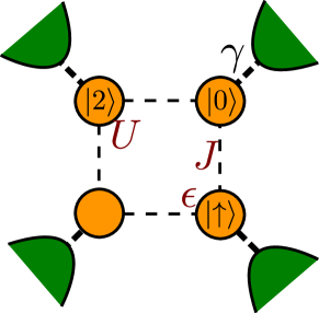
Figure 1: Sketch of a Fermi-Hubbard model (I) with four sites, where each site can host four states $\{\left|0\right>,\left|{\mathord{\uparrow}}\right>,\left|{\mathord{\downarrow}}\right>,\left|2\right>\}$, such that the system Hilbert space dimension is $4^{4}=256$. Between the sites, electronic tunnelling is possible with amplitude $J$. In absence of tunnelling, a single charge on a site (bottom right) will have an on-site energy $\epsilon$, whereas two electrons of opposite spin (top left) will have the energy $2\epsilon+U$. The local reservoirs may load and unload the system with bare rate $\gamma$.

Let us briefly discuss the region of applicability of this description. If we first consider disconnected lattice sites (i.e., $J=0$) weakly coupled to separate Markovian baths, such a master equation (2) can be derived in a standard way breuer2002 by considering sites and reservoirs separately. Now switching on the tunneling $J$ between lattice sites, an analogous derivation can be carried out, as we show in App. A, as long as the coupling $J$ between the lattice sites is weak in comparison to their coupling $\gamma$ to the reservoir – while both are much smaller than the interaction strength $U$.

The applicability of the underlying assumptions of separate or individual baths for each lattice site, as well as $J\ll\gamma$, depends on the specific physical realization. For ultra-cold atoms in optical lattices hofstetter2002a , the Mott-Hubbard system could be realized in a planar lattice while the separate baths correspond to atoms moving (guided by lasers) perpendicular to this plane – where the in-plane hopping strength $J$ can be tuned to be much smaller than the perpendicular tunneling strength which determines $\gamma$. For Fermi-Hubbard simulators based on gate-defined quantum dots hensgens2017a , local tunnelling reservoirs can be represented by smaller tunnel electrodes placed nearby. For other Hubbard systems sharing a common reservoir, the description based on separate baths can be a good approximation when the coupling to the lattice sites is effectively incoherent (e.g. if the lattice spacing of the Hubbard system is much larger than the relevant length scale, such as coherence or correlation length of the reservoir; or the bath relaxation is fast enough.)

II.1 Zero-temperature bath

As explained above, consistent with our assumption of a strongly interacting system, we assume that the on-site repulsion $U$ is not only much stronger than the system hopping $J$, but also dominant in comparison with the coupling to the bath. Apart from the spectral density of the reservoir, the impact of this coupling to the bath is mainly determined by the inverse temperature $\beta$ and the chemical potential $\mu_{\rm b}$ of the reservoir (which we assume to consist of free fermions). Let us first consider the case of zero temperature (cold bath), finite temperatures will be discussed in Sec VI below.

If the chemical potential of the bath is too low $\mu_{\rm b}<\epsilon$, all the particles from the system will just tunnel to the bath such that we are left with an empty system state. In the other limiting case, if the chemical potential is too high $\mu_{\rm b}>U+\epsilon$, the reservoir will fill up the system, also leading to a trivial state. Thus, we assume an intermediate chemical potential, for example $\mu_{\rm b}=\epsilon+U/2$, where only a doubly occupied site can release a particle into the reservoir due to its high on-site repulsion energy $U$, while singly occupied sites cannot do that as the reservoir states at the energy $\epsilon$ are already filled (Pauli principle). Conversely, only an empty lattice site can receive a particle from the bath. Altogether, a cold fermionic bath at intermediate chemical potential is described by two Lindblad operators for each site $\mu$ and spin $s$

$$\hat{L}_{I}\in\left\{\sqrt{\gamma}\,\left(1-\hat{n}_{\mu}^{\bar{s}}\right)\hat{c}_{\mu,s}^{\dagger}\,,\sqrt{\gamma}\,\hat{n}_{\mu}^{\bar{s}}\hat{c}_{\mu,s}\right\}\,,$$ (3)

where the double index $I=\{\mu,s\}$ comprises sites and spins. Here, $\bar{s}$ denotes the spin opposite to $s$ and $\gamma$ measures the strength of the coupling to the environment. Here, we assume that all these coupling strengths are the same, but one can also consider the case of different couplings $\gamma\to\gamma_{I}$.

III Relaxation Dynamics at $T=0$

Even though solving the full equation of motion (2) is only possible for very small lattices, we may gain interesting insight by considering special observables. For the total particle number $\hat{N}$, we find a fast relaxation towards half filling

$$\frac{d}{dt}\left<\hat{N}\right>=\frac{d}{dt}\sum_{\mu,s}\langle\hat{n}_{\mu}^{s}\rangle=-2\gamma\sum_{\mu,s}\left(\langle\hat{n}_{\mu}^{s}\rangle-\frac{1}{2}\right)\,.$$ (4)

Another interesting observable is the total angular momentum lieb1989a ; steeb1993a ; schumann2002a ; essler2005 ; pavarini2015

$$\hat{\mbox{\boldmath$S$}}=\sum_{\mu}\hat{\mbox{\boldmath$S$}}_{\mu}=\frac{1}{2}\sum_{\mu,s,s^{\prime}}\hat{c}^{\dagger}_{\mu,s}\mbox{\boldmath$\sigma$}_{s,s^{\prime}}\hat{c}_{\mu,s^{\prime}}$$ (5)

with the matrix elements of the Pauli matrices denoted by $\mbox{\boldmath$\sigma$}_{s,s^{\prime}}$. Its components obey the usual spin algebra $[\hat{S}^{x},\hat{S}^{y}]=\mathrm{i}\hat{S}^{z}$, and one can define the usual ladder operators via $\hat{S}^{\pm}=\hat{S}^{x}\pm\mathrm{i}\hat{S}^{y}$ that obey the commutation relations $[\hat{S}^{-},\hat{S}^{+}]=-2\hat{S}^{z}$ and $[\hat{S}^{z},\hat{S}^{\pm}]=\pm\hat{S}^{\pm}$. The unitary system dynamics generated by the Fermi-Hubbard Hamiltonian (I) in absence of a bath conserves this quantity $[\hat{H},\hat{\mbox{\boldmath$S$}}]=0$ (and therefore also $\hat{\mbox{\boldmath$S$}}^{2}$ is conserved for $\gamma=0$). After coupling to the zero-temperature bath discussed above (2), we still obtain an exact conservation law for the expectation value of the total spin $\hat{\mbox{\boldmath$S$}}$

$$\frac{d}{dt}\langle\hat{\mbox{\boldmath$S$}}\rangle=0\,.$$ (6)

Unlike in the unitary case however, its square is not conserved

$$\frac{d}{dt}\langle\hat{\mbox{\boldmath$S$}}^{2}\rangle=\frac{3\gamma}{2}\sum_{\mu}\langle\hat{n}_{\mu}^{\uparrow}\hat{n}_{\mu}^{\downarrow}+(1-\hat{n}_{\mu}^{\uparrow})(1-\hat{n}_{\mu}^{\downarrow})\rangle\geq 0\,.$$ (7)

Since the right-hand side of the above equation is non-negative, we find that $\langle\hat{\mbox{\boldmath$S$}}^{2}\rangle$ always grows until a steady state $\hat{\rho}_{\infty}$ is reached. Furthermore, we find that this steady state $\hat{\rho}_{\infty}$ must have exactly one particle per site such that $\langle\hat{n}_{\mu}^{\uparrow}\hat{n}_{\mu}^{\downarrow}\rangle=\langle(1-\hat{n}_{\mu}^{\uparrow})(1-\hat{n}_{\mu}^{\downarrow})\rangle=0$, i.e., the Mott insulator property is stable.

In addition to the total angular momentum $\hat{\mbox{\boldmath$S$}}$ discussed above, which can be defined for arbitrary lattice structures, we may introduce further relevant observables in bi-partite lattices. For these, we can find a site ordering $\mu$ such that the parity $(-1)^{\mu}$ is always opposite for neighboring lattice sites, which – in analogy to the spin – allows us to introduce the pseudo-spin operators yang1989a ; zhang1990a

$$\hat{\eta} =\sum_{\mu}(-1)^{\mu}\hat{c}_{\mu,\uparrow}\hat{c}_{\mu,\downarrow}\,,\quad\hat{\eta}_{z}=\frac{1}{2}\left(\hat{N}-N_{\rm lattice}\right)\,,$$ (8)

where $N_{\rm lattice}$ denotes the number of lattice sites. Analogous to the spin ladder operators, these obey the relations $[\hat{\eta},\hat{\eta}^{\dagger}]=-2\hat{\eta}_{z}$, $[\hat{\eta}_{z},\hat{\eta}]=-\hat{\eta}$, and $[\hat{\eta}_{z},\hat{\eta}^{\dagger}]=+\hat{\eta}^{\dagger}$. In contrast to Eq. (6), the pseudo-spin is not conserved in presence of a bath. The square of the total pseudo-spin is defined as

$$\hat{\mbox{\boldmath$\eta$}}^{2}=\frac{1}{2}\left(\hat{\eta}\hat{\eta}^{\dagger}+\hat{\eta}^{\dagger}\hat{\eta}\right)+\hat{\eta}_{z}^{2}\,,$$ (9)

and commutes with $\hat{H}$, $\hat{N}$, $\hat{\mbox{\boldmath$S$}}$, and $\hat{\mbox{\boldmath$S$}}^{2}$. It obeys a simple evolution equation quite analogous to Eq. (7)

$$\frac{d}{dt}\left<\hat{\mbox{\boldmath$\eta$}}^{2}\right> =\frac{3\gamma}{2}\sum_{\mu}\langle\hat{n}_{\mu}^{\uparrow}\hat{n}_{\mu}^{\downarrow}+(1-\hat{n}_{\mu}^{\uparrow})(1-\hat{n}_{\mu}^{\downarrow})\rangle$$

$$\qquad-4\gamma\left<\hat{\mbox{\boldmath$\eta$}}^{2}\right>\,.$$ (10)

Since the steady state $\hat{\rho}_{\infty}$ must have exactly one particle per site $\langle\hat{n}_{\mu}^{\uparrow}\hat{n}_{\mu}^{\downarrow}\rangle=\langle(1-\hat{n}_{\mu}^{\uparrow})(1-\hat{n}_{\mu}^{\downarrow})\rangle=0$, we see that $\left<\hat{\mbox{\boldmath$\eta$}}^{2}\right>$ must vanish in the steady state.

III.1 Steady states

Even without solving the full problem, we may infer some properties of the steady states albert2014a ; nigro2019a $\hat{\rho}_{\infty}$. Because they have exactly one particle per lattice site, the Lindblad operators $\hat{L}_{I}\hat{\rho}_{\infty}=0$ and the interaction term $\hat{H}_{U}\hat{\rho}_{\infty}=0$ acting on these states vanish identically while $\hat{H}_{\epsilon}$ acts trivially. Thus, it suffices to consider only the action of the hopping Hamiltonian $\hat{H}_{J}$ which can be diagonalized easily. Since those stationary states $\hat{\rho}_{\infty}$ must commute with $\hat{H}_{J}$, we may diagonalize them simultaneously. Then, because each term $\hat{c}^{\dagger}_{\mu,s}\hat{c}_{\nu,s}$ in the hopping Hamiltonian $\hat{H}_{J}$, after acting on a state with exactly one particle per lattice site, either annihilates this state or leads to a doubly occupied ($\mu$) and an empty ($\nu$) lattice site, these steady states $\hat{\rho}_{\infty}$ must also be in the sub-space with zero eigenvalue of the hopping Hamiltonian $\hat{H}_{J}$, i.e., $\hat{H}_{J}\hat{\rho}_{\infty}=0$. One example is the ferromagnetic state $\left|\uparrow\uparrow\uparrow\dots\right>$ which maximizes $\hat{S}_{z}$ and $\hat{\mbox{\boldmath$S$}}^{2}$ and is obviously a steady state. Now, as the ladder operators $\hat{S}_{\pm}$ commute with $\hat{H}$, we see that all the states $\left|\Psi_{n}\right>\propto\hat{S}_{-}^{n}\left|\uparrow\uparrow\uparrow\dots\right>$ are steady states. They maximize $\hat{\mbox{\boldmath$S$}}^{2}$ and form a ladder with $N_{\rm lattice}+1$ states from $\left|\uparrow\uparrow\uparrow\dots\right>$ to $\left|\downarrow\downarrow\downarrow\dots\right>$, whose rungs can be labeled by their different eigenvalues of $\hat{S}_{z}$.

III.2 Anti-ferromagnetic order

As we found above, the states with maximum $\hat{\mbox{\boldmath$S$}}^{2}$ are steady states. Note however, that the previous line of arguments does not necessarily imply that these are the only steady states – this depends on the lattice structure (which determines the diagonalization of $\hat{H}_{J}$). For a lattice which can be decomposed into two disconnected sub-lattices, for example, there are further steady states (which maximize $\hat{\mbox{\boldmath$S$}}^{2}$ for each sub-lattice separately).

However, the anti-ferromagnetic state (which is the ground state of $\hat{H}$ on simply connected bi-partite lattices) is not a steady state. As we have seen above, the steady states are annihilated by $\hat{H}_{J}$, i.e., all the hopping contributions vanish or cancel each other. In contrast, the anti-ferromagnetic order of the Mott-Néel state is precisely such that it facilitates tunneling in order to lower the energy cleveland1976a .

As a result, while the Mott insulator structure itself is stable (i.e., conserved by the steady states), we find a decay of the anti-ferromagnetic order of the Mott-Néel state due to the coupling to the environment according to Eq. (2).

III.3 Relaxation time scales

Finally, let us discuss the different time scales of relaxation. Obviously, the relaxation to half filling occurs on a time scale ${\cal O}(1/\gamma)$. In contrast, in the strongly interacting case $U\gg J$ at half filling, the right-hand side of (7) is suppressed as $J^{2}/U^{2}$ (as already mentioned in the introduction) and thus the growth in (7) is much slower than that in (4). As a result, we find two vastly different relaxation time scales – as already observed in many other systems and scenarios, see, e.g., Refs. queisser2014a ; queisser2019a ; kleinherbers2020a ; wu2020a ; avigo2020a ; wang2020a . A more quantitative analysis of these two time scales will be presented in the next section.

IV Waiting Time Distribution

In order to study the different time scales observed above in more detail, let us re-write the master equation (2) in terms of the Liouville super-operator $\cal L$

$$\frac{d\hat{\rho}}{dt}=-\mathrm{i}\hat{H}_{\rm eff}\hat{\rho}+\mathrm{i}\hat{\rho}\hat{H}_{\rm eff}^{\dagger}+\sum_{I}\hat{L}_{I}\hat{\rho}\hat{L}_{I}^{\dagger}={\cal L}\hat{\rho}\,,$$ (11)

where we have introduced the effective Hamiltonian

$$\hat{H}_{\rm eff}=\hat{H}-\frac{\mathrm{i}}{2}\,\sum_{I}\hat{L}_{I}^{\dagger}\hat{L}_{I}=\hat{H}-\frac{\mathrm{i}}{2}\,\hat{\mbox{\boldmath$L$}}^{2}\,,$$ (12)

which is non-Hermitian due to the coupling with the bath. For the cold bath (3), we find

$$\hat{\mbox{\boldmath$L$}}^{2}=-2\gamma\sum_{\mu,s}\left(\hat{n}_{\mu}^{s}-\frac{1}{2}\right)+4\gamma\sum_{\mu}\hat{n}_{\mu}^{\uparrow}\hat{n}_{\mu}^{\downarrow}\,.$$ (13)

Thus, apart from the c-number contribution, the effective Hamiltonian (12) has the same structure as the Fermi-Hubbard model (I), just with complex parameters $U\to U-2\mathrm{i}\gamma$ and $\epsilon\to\epsilon+\mathrm{i}\gamma$.

As the next step, we decompose the total Liouville super-operator $\cal L$ into the jump term

$${\cal L}_{\rm jump}\hat{\rho}=\sum_{I}\hat{L}_{I}\hat{\rho}\hat{L}_{I}^{\dagger}$$ (14)

and remaining contribution ${\cal L}_{\rm stay}={\cal L}-{\cal L}_{\rm jump}$ corresponding to no jumps. Then, the total evolution of the density matrix $\hat{\rho}$ in a time interval $[0,t]$ can be expanded into a Dyson series in ${\cal L}_{\rm jump}$ via

$$e^{{\cal L}t}=e^{{\cal L}_{\rm stay}t}+\int_{0}^{t}dt^{\prime}\,e^{{\cal L}_{\rm stay}(t-t^{\prime})}{\cal L}_{\rm jump}e^{{\cal L}_{\rm stay}t^{\prime}}+\dots$$ (15)

The first term $e^{{\cal L}_{\rm stay}t}$ corresponds to no jumps in time interval $[0,t]$, the second term describes one jump at a time $t^{\prime}$ and the higher-order contributions correspond to two or more jumps. As a result, starting with the initial state $\hat{\rho}_{0}=\hat{\rho}(t=0)$, the probability for no jump during the time interval $[0,t]$ is given by

$$P_{\rm stay}(t)={\rm Tr}\left\{e^{{\cal L}_{\rm stay}t}\hat{\rho}_{0}\right\}={\rm Tr}\left\{e^{-\mathrm{i}\hat{H}_{\rm eff}t}\hat{\rho}_{0}e^{+\mathrm{i}\hat{H}_{\rm eff}^{\dagger}t}\right\}.$$ (16)

This allows us to infer the waiting time distribution cohen_tannouji1986a ; plenio1998a ; brandes2008a ; albert2011a ; albert2012a ; rajabi2013a ; sothmann2014a ; ptaszynski2017a ; kleinherbers2021a , i.e., the probability density $\omega(t)$ of the waiting time $t$ until an initial state $\hat{\rho}_{0}$ decays due to the first jump, via

$$\omega(t)=-\dot{P}_{\rm stay}\,.$$ (17)

This waiting time distribution is a quantitative measure of the relaxation rates and its decay constants are determined by the complex eigenvalues $\sigma_{n}$ of $\hat{H}_{\rm eff}$ via $e^{-\mathrm{i}H_{\rm eff}t}=\sum_{n}{\hat{M}}_{n}(t)e^{-\mathrm{i}\sigma_{n}t}$, where the ${\hat{M}}_{n}(t)$ can (for degenerate $\sigma_{n}$) be polynomial functions of $t$. Thus, the imaginary parts $\Im{\sigma_{n}}\leq 0$ in particular determine the decay characteristics of the waiting time distributions.

A first rough estimate of these eigenvalues of $\hat{H}_{\rm eff}$ can be obtained by perturbation theory in $\gamma$. Note that perturbation theory for non-Hermitian operators (such as $\hat{H}_{\rm eff}$) is typically more complicated than for Hermitian operators (such as $\hat{H}$) buth2004a ; Ashida2020 . Nevertheless, starting from the undisturbed eigenstates $\left|u_{\lambda}\right>$ of the Fermi-Hubbard Hamiltonian $\hat{H}$ corresponding to the real undisturbed (and assumed to be non-degenerate) eigenvalues $\lambda$, we may find the first-order shift of the associated complex eigenvalues $\sigma_{\lambda}$ of $\hat{H}_{\rm eff}$ by

$$\sigma_{\lambda}=\lambda-\frac{\mathrm{i}}{2}\left<u_{\lambda}\right|\hat{\mbox{\boldmath$L$}}^{2}\left|u_{\lambda}\right>+{\cal O}(\gamma^{2})\,.$$ (18)

For example, the empty state $\left|u_{\lambda}\right>=\left|00\dots\right>$ with $\lambda=0$ is shifted to the imaginary eigenvalue $\sigma_{\lambda}=-\mathrm{i}\gamma N_{\rm lattice}$ with $N_{\rm lattice}$ denoting the number of lattice sites – which corresponds to the fast relaxation of the particle number (4). As another example, the aforementioned ferromagnetic state $\left|u_{\lambda}\right>=\left|\uparrow\uparrow\dots\right>$ is inert and thus has no imaginary shift $\Im(\sigma_{\lambda})=0$, showing that it is a steady state (at zero temperature).

The evaluation of waiting times between two jumps is also possible brandes2008a ; albert2011a , and can analogously be achieved by evaluating the exponential of $\hat{H}_{\rm eff}$.

V Hubbard Tetramer at $T=0$

The above approach based on the waiting-time distribution goes along with a tremendous reduction in complexity. Instead of calculating $e^{{\cal L}t}$ or diagonalizing $\cal L$, it suffices to diagonalize the effective Hamiltonian $\hat{H}_{\rm eff}$. Moreover, we found that $\hat{H}_{\rm eff}$ has the same structure as the original Fermi-Hubbard Hamiltonian $\hat{H}$, just with complex parameters $U$ and $\epsilon$. Of course, despite this reduction in complexity, one can only derive general analytic expressions in those cases where the original Fermi-Hubbard Hamiltonian $\hat{H}$ can be diagonalized.

In order to treat such a simple (yet non-trivial) case, we consider the Fermi-Hubbard model on a square (which is equivalent to a ring consisting of 4 lattice sites). Even in this simple case, the total Hilbert space contains $4^{4}=256$ states, i.e., $\hat{H}_{\rm eff}$ and $\hat{H}$ can be represented as $256\times 256$-matrices. In order to bring these matrices into a treatable block-diagonal form, we employ a suitable set of commuting observables.

Apart from the total particle number $\hat{N}$, we select $\hat{S}_{z}$ and $\hat{\mbox{\boldmath$S$}}^{2}$ as further commuting observables. The total spin $\hat{\mbox{\boldmath$S$}}^{2}$ allows us to classify the Hubbard tetramer spectrum into 42 singlets, 48 doublets, 27 triplets, 8 quadruplets, and 1 quintuplet. These states compose the $42\cdot 1+48\cdot 2+27\cdot 3+8\cdot 4+1\cdot 5=256$ states in the total Hilbert space. In analogy to the spin $\hat{\mbox{\boldmath$S$}}^{2}$, the pseudo-spin (9) also allows to classify the 256 states into $42$ pseudo-singlets, $48$ pseudo-doublets, $27$ pseudo-triplets, $8$ pseudo-quadruplets, and $1$ pseudo-quintuplet. The classification according to the pseudo-spin is different from that according to the spin, which allows us to decompose the Hilbert space further.

As the final ingredient, we use suitable geometric symmetries of the square. One option could be the quasi-momentum which generates the cyclic permutation $\hat{P}_{1234}$: $1\to 2$, $2\to 3$, $3\to 4$ and $4\to 1$ of the lattice sites, see App. B. However, we found it more convenient to employ the reflections at the two diagonals of the square, i.e., the permutations $\hat{P}_{13}$ and $\hat{P}_{24}$

$$\hat{P}_{\mu\nu}=\exp\left\{\mathrm{i}\frac{\pi}{2}\sum_{s}\left(\hat{c}_{\mu,s}^{\dagger}\hat{c}_{\nu,s}+\hat{c}_{\nu,s}^{\dagger}\hat{c}_{\mu,s}-\hat{n}_{\mu,s}-\hat{n}_{\nu,s}\right)\right\}\,,$$

exchanging sites $1\leftrightarrow 3$ and $2\leftrightarrow 4$, respectively. These symmetry operations represent additional commuting observables with eigenvalues (parities) $\pm 1$.

Now we may use the set $\{\hat{N},\hat{S}_{z},\hat{\mbox{\boldmath$S$}}^{2},\hat{\mbox{\boldmath$\eta$}}^{2},\hat{P}_{13},\hat{P}_{24}\}$ to diagonalize $\hat{H}_{\rm eff}$, which can be decomposed into independent blocks with maximum rank four, which allows us to find the eigenvalues analytically. For example, the empty state $\left|0000\right>$ lies in the sector with even parities where all the other quantities $\{\hat{N},\hat{S}_{z},\hat{\mbox{\boldmath$S$}}^{2},\hat{\mbox{\boldmath$\eta$}}^{2}\}$ vanish. It is an eigenstate of $\hat{H}_{\rm eff}$ with the eigenvalue $\sigma=-4\mathrm{i}\gamma$, and its waiting-time distribution correspondingly reads

$$w(t)=-\dot{P}_{\rm stay}(t)=8\gamma e^{-8\gamma t}\,.$$ (20)

As already explained above, the quintuplet states are steady states

$$\left|\Psi_{-2}\right> =\left|{\mathord{\downarrow}}{\mathord{\downarrow}}{\mathord{\downarrow}}{\mathord{\downarrow}}\right>\,,$$

$$\left|\Psi_{-1}\right> =\frac{1}{2}\left[\left|{\mathord{\uparrow}}{\mathord{\downarrow}}{\mathord{\downarrow}}{\mathord{\downarrow}}\right>+\left|{\mathord{\downarrow}}{\mathord{\uparrow}}{\mathord{\downarrow}}{\mathord{\downarrow}}\right>+\left|{\mathord{\downarrow}}{\mathord{\downarrow}}{\mathord{\uparrow}}{\mathord{\downarrow}}\right>+\left|{\mathord{\downarrow}}{\mathord{\downarrow}}{\mathord{\downarrow}}{\mathord{\uparrow}}\right>\right]\,,$$

$$\left|\Psi_{0}\right> =\frac{1}{\sqrt{6}}\Big{[}\left|{\mathord{\uparrow}}{\mathord{\uparrow}}{\mathord{\downarrow}}{\mathord{\downarrow}}\right>+\left|{\mathord{\uparrow}}{\mathord{\downarrow}}{\mathord{\uparrow}}{\mathord{\downarrow}}\right>+\left|{\mathord{\uparrow}}{\mathord{\downarrow}}{\mathord{\downarrow}}{\mathord{\uparrow}}\right>$$

$$\qquad+\left|{\mathord{\downarrow}}{\mathord{\uparrow}}{\mathord{\uparrow}}{\mathord{\downarrow}}\right>+\left|{\mathord{\downarrow}}{\mathord{\uparrow}}{\mathord{\downarrow}}{\mathord{\uparrow}}\right>+\left|{\mathord{\downarrow}}{\mathord{\downarrow}}{\mathord{\uparrow}}{\mathord{\uparrow}}\right>\Big{]}\,,$$

$$\left|\Psi_{+1}\right> =\frac{1}{2}\left[\left|{\mathord{\downarrow}}{\mathord{\uparrow}}{\mathord{\uparrow}}{\mathord{\uparrow}}\right>+\left|{\mathord{\uparrow}}{\mathord{\downarrow}}{\mathord{\uparrow}}{\mathord{\uparrow}}\right>+\left|{\mathord{\uparrow}}{\mathord{\uparrow}}{\mathord{\downarrow}}{\mathord{\uparrow}}\right>+\left|{\mathord{\uparrow}}{\mathord{\uparrow}}{\mathord{\uparrow}}{\mathord{\downarrow}}\right>\right]\,,$$

$$\left|\Psi_{+2}\right> =\left|{\mathord{\uparrow}}{\mathord{\uparrow}}{\mathord{\uparrow}}{\mathord{\uparrow}}\right>\,,$$ (21)

and thus their waiting-time distributions vanish identically $w(t)=0$. They all contain four particles with maximum $\hat{\mbox{\boldmath$S$}}^{2}$ and are labeled by their $\hat{S}_{z}$ eigenvalues. All these states have odd parities (due to the Pauli principle) and are annihilated by $\hat{\mbox{\boldmath$\eta$}}^{2}$, i.e., ${\left|\eta\right|}=0$. For the Hubbard tetramer, these are the only steady states.

For the Hubbard dimer, we found in Ref. kleinherbers2020a a slow relaxation for the spin singlet state $(\left|\uparrow\downarrow\right>-\left|\downarrow\uparrow\right>)/\sqrt{2}$. Thus, let us now consider its straight-forward generalization to four lattice sites

$$\left|\Psi_{\rm zaf}\right>=\frac{\left|\uparrow\downarrow\uparrow\downarrow\right>-\left|\downarrow\uparrow\downarrow\uparrow\right>}{\sqrt{2}}\,.$$ (22)

This state displays Ising type (i.e., $\hat{S}_{z}$) anti-ferromagnetic order and lies in the sector with $N=4$ particles, ${\left|S\right|}=1$, $S_{z}=0$, and ${\left|\eta\right|}=0$ and is separately odd under the site permutations $\hat{P}_{13}$ and $\hat{P}_{24}$. This sector contains  two additional states $\left|\Psi_{\rm zaf}^{1}\right>$ and $\left|\Psi_{\rm zaf}^{2}\right>$ that can be conveniently generated from $\left|\Psi_{\rm zaf}\right>$ by acting with the hopping Hamiltonian $\hat{H}_{J}$ and subsequent Erhard-Schmidt orthogonalization .

In the basis $\{\left|\Psi_{\rm zaf}^{0}\right>=\left|\Psi_{\rm zaf}\right>,\left|\Psi_{\rm zaf}^{1}\right>,\left|\Psi_{\rm zaf}^{2}\right>\}$,the effective Hamiltonian can be represented by the $3\times 3$-matrix (the signs of off-diagonal matrix elements can be controlled by properly choosing the basis vectors)

$$\hat{H}_{\rm eff}=\left(\begin{array}[]{ccc}4\epsilon&+\sqrt{8}J&0\\ +\sqrt{8}J&4\epsilon+U-2\mathrm{i}\gamma&+\sqrt{8}J\\ 0&+\sqrt{8}J&4\epsilon+U-2\mathrm{i}\gamma\end{array}\right)\,.$$ (26)

The eigenvalues of this matrix reflect the two relaxation times scales mentioned above. In the strongly interacting limit $U\gg J$, two eigenvalues $\sigma_{\pm}$ have a large imaginary part $\Im(\sigma_{\pm})\approx-2\gamma$ while the remaining eigenvalue $\sigma_{0}$ – whose eigenvector has the largest overlap with the anti-ferromagnetic state (22) – has much smaller imaginary part $\Im(\sigma_{0})={\cal O}(\gamma J^{2}/U^{2})$. Specifically, a Taylor expansion in $J/U\ll 1$ up to quadratic order yields

$$\sigma_{0} \approx 4\epsilon-\frac{8J^{2}}{U}-\mathrm{i}\frac{16\gamma J^{2}}{U^{2}}\,,$$ (27)

$$\sigma_{\pm} \approx 4\epsilon+U\pm 2\sqrt{2}J+\frac{4J^{2}}{U}+\mathrm{i}\left(-2\gamma+\frac{8\gamma J^{2}}{U^{2}}\right)\,.$$

Finally, let us consider the full Heisenberg type anti-ferromagnetic state, i.e., the Mott-Néel state

$$\left|\Psi_{\rm af}\right> =\frac{1}{\sqrt{12}}\big{[}2\left|{\mathord{\uparrow}}{\mathord{\downarrow}}{\mathord{\uparrow}}{\mathord{\downarrow}}\right>+2\left|{\mathord{\downarrow}}{\mathord{\uparrow}}{\mathord{\downarrow}}{\mathord{\uparrow}}\right>$$

$$\qquad-\left|{\mathord{\uparrow}}{\mathord{\uparrow}}{\mathord{\downarrow}}{\mathord{\downarrow}}\right>-\left|{\mathord{\uparrow}}{\mathord{\downarrow}}{\mathord{\downarrow}}{\mathord{\uparrow}}\right>-\left|{\mathord{\downarrow}}{\mathord{\downarrow}}{\mathord{\uparrow}}{\mathord{\uparrow}}\right>-\left|{\mathord{\downarrow}}{\mathord{\uparrow}}{\mathord{\uparrow}}{\mathord{\downarrow}}\right>\big{]}\,,$$ (28)

which is orthogonal to the previously discussed states (V) and (22). It belongs to the sector with $N=4$, $S_{z}=0$, ${\left|S\right|}=0$, ${\left|\eta\right|}=0$, and is separately odd under the site permutations $\hat{P}_{13}$ and $\hat{P}_{24}$. As before, this sector contains two additional states that can be created by the action of $\hat{H}_{J}$ and subsequent orthonormalization , and in the basis formed by $\{\left|\Psi_{\rm af}^{0}\right>=\left|\Psi_{\rm af}\right>,\left|\Psi_{\rm af}^{1}\right>,\left|\Psi_{\rm af}^{2}\right>\}$, the effective non-Hermitian Hamiltonian has the representation

$$\hat{H}_{\rm eff} =\left(\begin{array}[]{ccc}4\epsilon&\sqrt{12}J&0\\ \sqrt{12}J&4\epsilon+U-2\mathrm{i}\gamma&2J\\ 0&2J&4\epsilon+2U-4\mathrm{i}\gamma\end{array}\right)\,.$$ (32)

Taylor expansion for $J/U\ll 1$ yields the eigenvalues

$$\sigma_{0} \approx 4\epsilon-12\frac{J^{2}}{U}-\mathrm{i}\frac{24\gamma J^{2}}{U^{2}}\,,$$

$$\sigma_{1} \approx 4\epsilon+U+8\frac{J^{2}}{U}+\mathrm{i}\left(-2\gamma+\frac{16\gamma J^{2}}{U^{2}}\right)\,,$$

$$\sigma_{2} \approx 4\epsilon+2U+4\frac{J^{2}}{U}+\mathrm{i}\left(-4\gamma+\frac{8\gamma J^{2}}{U^{2}}\right)\,,$$ (33)

which now has three distinct modes, two fast decaying ones and a slower decaying one.

Retrieving the isolated Fermi-Hubbard model by considering the real part of Eqns. (27) and (V), we see that the lowest energy state comes from the sector described by matrix representation (32), and indeed one can show that the ground state in the sector with $N_{{\mathord{\uparrow}}}=N_{{\mathord{\downarrow}}}=2$ is spanned by the states $\left|\Psi_{\rm af}^{0}\right>$ and (for $J\ll U$ small) contributions of $\left|\Psi_{\rm af}^{1}\right>$ and $\left|\Psi_{\rm af}^{2}\right>$. Indeed, it is well-known lieb1989a that the ground state of the half-filled sector must have $\langle\hat{\mbox{\boldmath$S$}}^{2}\rangle=0$. Given the evident anti-ferromagnetic order of (22), this may appear surprising but one should keep in mind that the true ground state maximizes the full (Heisenberg type) anti-ferromagnetic order operator

$$\hat{O}_{\rm af}=-\sum_{\mu=1}^{4}\hat{\mbox{\boldmath$S$}}_{\mu}\cdot\hat{\mbox{\boldmath$S$}}_{\mu+1}\,,$$ (34)

which is directly proportional to a Heisenberg Hamiltonian. This order operator commutes with $\hat{N}$, $\hat{S}_{z}$, $\hat{\mbox{\boldmath$S$}}^{2}$, and the quasi-momentum $\hat{P}_{1234}$ or the permutation operators $\hat{P}_{13}$ and $\hat{P}_{24}$, it can therefore also be brought in the same block-diagonal form as $\hat{H}_{\rm eff}$. Direct inspection of $\left<\Psi_{\rm af}\left|\hat{O}_{\rm af}\right|\Psi_{\rm af}\right>=2$ shows that $\left|\Psi_{\rm af}\right>$ is maximally ordered, and thereby more ordered than $\left|\Psi_{\rm zaf}\right>$, for which one finds $\left<\Psi_{\rm zaf}\left|\hat{O}_{\rm af}\right|\Psi_{\rm zaf}\right>=1$. Even for finite but small $J/U$, the ground states (for $\gamma=0$) of Eqns. (26) and (32) possess the order parameters $\langle\hat{O}_{\rm af}\rangle\approx 1-10J^{2}/U^{2}$ and $\langle\hat{O}_{\rm af}\rangle\approx 2-15J^{2}/U^{2}$, respectively. One can show that these expectation values are consistent with the lowest eigenvalues (27) and (V) of the isolated tetramer, for which an effective Heisenberg-type Hamiltonian applies cleveland1976a , see App. C.

In an analogous fashion, the decay properties of all eigenstates of the Hubbard model on the square can be analytically evaluated. For illustration, we provide the qualitative decay dynamics of all $36$ states in the sector $N_{\mathord{\uparrow}}=2=N_{\mathord{\downarrow}}$ in App. D.

VI Finite-temperature bath

For finite reservoir temperatures, the calculations are essentially analogous, we just have to take the finite occupations of the reservoir into account. Then, the Lindblad operators in (3) generalize to four operators per site and spin

$$\hat{L}_{I} \in\Big{\{}\sqrt{\gamma f_{\rm E}}(1-\hat{n}_{\mu}^{\bar{s}})\hat{c}_{\mu,s}^{\dagger},\sqrt{\gamma(1-f_{\rm E})}(1-\hat{n}_{\mu}^{\bar{s}})\hat{c}_{\mu,s}\,,$$

$$\qquad\sqrt{\gamma f_{\rm U}}\hat{n}_{\mu}^{\bar{s}}\hat{c}_{\mu,s}^{\dagger},\sqrt{\gamma(1-f_{\rm U})}\hat{n}_{\mu}^{\bar{s}}\hat{c}_{\mu,s}\Big{\}}\,,$$ (35)

which we motivate microscopically in App. E. Here, the thermal properties of the reservoir are encoded in the Fermi functions for transitions between empty (E) and singly-charged dots $f_{\rm E}=[e^{\beta(\epsilon-\mu_{\rm b})}+1]^{-1}$ and for transitions between singly and doubly charged (U) dots $f_{\rm U}=[e^{\beta(\epsilon+U-\mu_{\rm b})}+1]^{-1}$, with inverse temperature $\beta$ and chemical potential $\mu_{\rm b}$ while $\gamma$ denotes the spectral density (assumed flat over the energy scales of the tetramer, wideband limit). The first Lindblad operator above describes a transfer of an electron with spin $s$ onto site $\mu$, provided the other spin species $\bar{s}$ is not present at that site and the second term describes the reverse process, i.e., an electron with spin $s$ leaving site $\mu$ when the other spin species is not present. The second line above describes the same processes when the other spin species is present, where the corresponding transition rates are modified by the Coulomb interaction. When $\mu_{\rm b}=\epsilon+U/2$ and $\beta U\gg 1$, we get $f_{\rm E}\to 1$ and $f_{\rm U}\to 0$, such that the previous Lindblad operators (3) are reproduced. The generator (2) with Lindblad operators (VI) tends to locally thermalize the system, i.e., in the limit $J=0$ the state $\hat{\rho}_{\beta}\propto\exp\left\{-\beta(\hat{H}_{\epsilon}+\hat{H}_{U}-\mu_{\rm b}\hat{N})\right\}$ is a stationary state.

To identify the non-Hermitian Hamiltonian, we evaluate

$$\hat{\mbox{\boldmath$L$}}^{2} =\sum_{\mu s}\Big{[}\gamma f_{\rm E}(\mbox{\boldmath$1$}-\hat{n}_{\mu}^{\bar{s}})(\mbox{\boldmath$1$}-\hat{n}_{\mu}^{s})+\gamma(1-f_{\rm E})(\mbox{\boldmath$1$}-\hat{n}_{\mu}^{\bar{s}})\hat{n}_{\mu}^{s}$$

$$\qquad+\gamma f_{\rm U}\hat{n}_{\mu}^{\bar{s}}(\mbox{\boldmath$1$}-\hat{n}_{\mu}^{s})+\gamma(1-f_{\rm U})\hat{n}_{\mu}^{\bar{s}}\hat{n}_{\mu}^{s}\Big{]}$$

$$=2N_{\rm lattice}\gamma f_{\rm E}\mbox{\boldmath$1$}+\gamma(1+f_{\rm U}-3f_{\rm E})\sum_{\mu s}\hat{n}_{\mu}^{s}$$

$$\qquad+4\gamma(f_{\rm E}-f_{\rm U})\sum_{\mu s}\hat{n}_{\mu}^{\bar{s}}\hat{n}_{\mu}^{s}\,.$$ (36)

Thus, apart from a shift of $-N_{\rm lattice}\mathrm{i}\gamma f_{\rm E}$, the effective non-Hermitian Hamiltonian contains the on-site energy $\epsilon\to\epsilon-\mathrm{i}\gamma/2(1+f_{\rm U}-3f_{\rm E})$ and the Coulomb interaction $U\to U-2\mathrm{i}\gamma(f_{\rm E}-f_{\rm U})$ as complex parameters also for finite temperatures. The previously discussed zero-temperature limit (when $\mu_{\rm b}=\epsilon+U/2$ and $\beta U\gg 1$) is recovered by $f_{\rm E}\to 1$ and $f_{\rm U}\to 0$.

VI.1 Infinite temperature limit

At infinite temperatures, we just set $f_{\rm E}\to 1/2$ and $f_{\rm U}\to 1/2$, and the effective non-Hermitian Hamiltonian is trivially shifted $\hat{H}_{\rm eff}=\hat{H}-\frac{\mathrm{i}}{2}\gamma N_{\rm lattice}\mbox{\boldmath$1$}$. Explicit evaluation of the master equation (2) with Lindblad operators (VI) then shows that $\hat{\rho}_{\infty}\propto\mbox{\boldmath$1$}$ is a stationary state at infinite temperatures. Consistently, we find that in this limit observables that are conserved for the isolated Fermi-Hubbard model obey simple closed equations of motion. For example, the particle number again decays quickly towards half filling, but the relaxation rate is only half that of the low-temperature limit (4)

$$\frac{d}{dt}\sum_{\mu,s}\left<\hat{n}_{\mu}^{s}\right>=-\gamma\left(\sum_{\mu,s}\left<\hat{n}_{\mu}^{s}\right>-\frac{1}{2}\right)\,.$$ (37)

The spin components are no longer conserved as in (6) but decay according to

$$\frac{d}{dt}\left<\hat{\mbox{\boldmath$S$}}\right>=-\gamma\left<\hat{\mbox{\boldmath$S$}}\right>\,.$$ (38)

Analogously, in contrast to (7), the spin quadrature decays according to

$$\frac{d}{dt}\left<\hat{\mbox{\boldmath$S$}}^{2}\right>=-2\gamma\left(\left<\hat{\mbox{\boldmath$S$}}^{2}\right>-\frac{3}{2}\right)\,.$$ (39)

The stationary value $3/2$ of the spin quadrature is consistent with $\hat{\rho}_{\infty}\propto\mbox{\boldmath$1$}$.

Furthermore, in contrast to (III), the pseudo-spin evolves similarly to the spin

$$\frac{d}{dt}\left<\hat{\mbox{\boldmath$\eta$}}^{2}\right>=-2\gamma\left(\left<\hat{\mbox{\boldmath$\eta$}}^{2}\right>-\frac{3}{2}\right)\,.$$ (40)

One may ask how the interacting Lindblad operators (VI) are compatible with the following phenomenological picture kleinherbers2020a : For infinite temperatures, due to availability of the full range of energies, one might expect that the model behaves as independent sites which can be loaded and unloaded just as non-interacting electrons, i.e., independent of whether an electron is already present or not. Closer inspection shows that for states $\hat{\rho}$ obeying $\left[\hat{\rho},\hat{n}_{\mu}^{s}\right]=0$ (e.g., having definite particle numbers $\hat{n}_{\mu}^{s}$ for each site $\mu$ and spin $s$), one may recombine the dissipators (VI) to recover the local description of independent electrons – formally equivalent to Eq. (E) for $f=1/2$, which would also result from the coherent approximation introduced in Ref. kleinherbers2020a . This does of course depend on the initial state, and it is indeed an interesting route of further research to investigate how the decay dynamics depends on the presence of correlations.

VI.2 Hubbard tetramer

For finite temperatures and finite chemical potentials the initially empty ($E$) and initially filled ($F$) states decay trivially

$$\omega_{E}(\tau) =8\gamma f_{\rm E}e^{-8\gamma\tau f_{\rm E}}\,,$$

$$\omega_{F}(\tau) =8\gamma(1-f_{\rm U})e^{-8\gamma\tau(1-f_{\rm U})}\,.$$ (41)

In general, when we consider states that are completely determined by the known quantum numbers, the effective non-Hermitian Hamiltonian will be a $1\times 1$-matrix, which only allows the waiting-time distribution to decay in a simple exponential fashion. For example, the five quintuplett states (V) that are completely determined by fixing $\hat{\mbox{\boldmath$S$}}^{2}$ and $\hat{S}_{z}$ and superpositions of them all obey the same waiting time distribution

$$\omega_{2}(\tau)=4\gamma(1-f_{\rm E}+f_{\rm U})e^{-4\gamma\tau(1-f_{\rm E}+f_{\rm U})}\,.$$ (42)

As mentioned, for $\mu_{\rm b}=\epsilon+U/2$, these states remain stable in the zero-temperature limit $\beta U\gg 1$. For small but finite temperatures, we find that $1-f_{\rm E}+f_{\rm U}\approx 2e^{-\beta U/2}$, such that their average lifetime scales as

$$\left<\tau\right>=\int_{0}^{\infty}\tau\omega_{2}(\tau)d\tau\approx\frac{e^{U\beta/2}}{8\gamma}\,.$$ (43)

One could imagine to exploit this very long lifetime for storing (quantum) information in superpositions of these states at low temperatures. However, as the waiting time distribution (42) is a simple exponential decay, it offers no lifetime guarantee, i.e., arbitrarily short lifetimes are possible (and actually always more probable than long ones).

Note that this is different for the state (22), for which the effective non-Hermitian Hamiltonian assumes nearly the same form as for zero temperatures, the only difference to Eq. (26) is that the top-left matrix element is modified to

$$\left<\Psi_{\rm zaf}^{0}\right|\hat{H}_{\rm eff}\left|\Psi_{\rm zaf}^{0}\right>=4\epsilon-2\mathrm{i}\gamma(1+f_{\rm U}-f_{\rm E})\,,$$ (44)

where we again reproduce the previous case at low temperatures and half-filling potential ($f_{\rm E}\to 1$ and $f_{\rm U}\to 0$). The situation is however fundamentally different in the infinite temperature limit ($f_{\rm E}=f_{\rm U}=1/2$), where the eigenvalues of $H_{\rm eff}$ are just the eigenvalues of $\hat{H}$ shifted by $-2\mathrm{i}\gamma$ towards the lower complex plane. Thus, at high temperatures this state will decay in a trivial exponential fashion $\propto e^{-4\gamma t}$, whereas at low temperatures the competing much slower timescale from (27) is revealed.

For the fully anti-ferromagnetic state (V), we find that in Eq. (32) two matrix elements have to be modified

$$\left<\Psi_{\rm af}^{0}\right|\hat{H}_{\rm eff}\left|\Psi_{\rm af}^{0}\right> =4\epsilon-2\mathrm{i}\gamma(1+f_{\rm U}-f_{\rm E})\,,$$

$$\left<\Psi_{\rm af}^{2}\right|\hat{H}_{\rm eff}\left|\Psi_{\rm af}^{2}\right> =4\epsilon+2U-2\mathrm{i}\gamma(1+f_{\rm E}-f_{\rm U})\,,$$ (45)

such that also here at high temperatures all modes decay similarly.

The resulting waiting time distributions for the states (22) and (V) are displayed for different temperatures in Fig. 2.

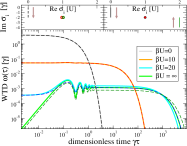
Figure 2: Main: Waiting time distribution (WTD) for state $\left|\Psi_{\rm zaf}\right>$ from Eq. (22) (dashed curves) and state $\left|\Psi_{\rm af}\right>$ from Eq. (V) (solid curves) for different temperatures. For high temperatures, one has a trivial exponential decay and both states decay virtually identically, cf. the solid gray and dashed black curves for $\beta U=0$ as well as the solid orange and dashed red curves for $\beta U=10$. For lower temperatures, oscillations appear and differences between the curves become visible, cf. the solid light blue and the dashed dark blue curves for $\beta U=20$ as well as solid light green and dashed dark green curves at zero temperature. For the latter case, the waiting time distribution at small times vanishes, making an immediate decay of the anti-ferromagnetic states unlikely. Top: Parametric plots of the corresponding exact eigenvalues of $\hat{H}_{\rm eff}$ as a function of temperature. For sector (26) in the top left panel, one eigenvalue (dashed black line) moves downwards with rising temperature (brown arrow), whereas the other two remain rather inert (sketched by the red and green hollow circles in the center). For sector (32) in the top right panel, one eigenvalue (black solid line) moves downwards and another (green solid line) upwards as the temperature increases (brown arrows), whereas the remaining one remains approximately inert (red circle). However, the anti-ferromagnetically ordered states always decay (the area under all curves of the main plot is one and all eigenvalues remain in the lower complex plane). Other parameters: $\epsilon=0$, $J=U/200$, $\gamma=U/20$, $\mu_{\rm b}=U/2$.

One can see that the differences between the waiting time distributions for the two anti-ferromagnetic states are small and become visible only at very small temperatures. Both states can at small temperatures be equipped with a lifetime guarantee (meaning that short lifetimes are less probable or formally that $\omega(\tau)$ vanishes at small $\tau$), in contrast to the trivially decaying quintuplet states.

VII Summary

We analyzed the relaxation dynamics of the open Fermi-Hubbard model as a prototypical example for a strongly interacting quantum many-body system subject to local dissipation. More precisely, we considered the limit of large on-site Coulomb repulsion $U$ and small intra-system hopping strength $J$. In order to model the environment, each lattice site is tunnel coupled to a (separate) free fermionic reservoir. In this regime, dissipation can be described by a simple Lindblad master equation which is local in time and space. As a result, we were able to find simple evolution equations for several observables, such as total particle number and total angular momentum, which are valid for arbitrary lattices. For zero-temperature reservoirs, these evolution equations already indicate the emergence of very different relaxation time scales, as also found in other examples  queisser2014a ; queisser2019a ; kleinherbers2020a ; wu2020a ; avigo2020a ; wang2020a , see Fig. 3.

These different relaxation time scales can be made more explicit in terms of waiting-time distributions describing the probability of a jump (i.e., a tunneling event between system and reservoir) in a given time interval, see Fig. 3. Employing a description of the no-jump evolution by an effective non-Hermitian Hamiltonian, we derived an explicit expression of the waiting-time distributions. This effective non-Hermitian Hamiltonian has the same symmetries as the original Fermi-Hubbard Hamiltonian steeb1993a ; schumann2002a and can thus be block-diagonalized in basically the same way – yielding a tremendous reduction in complexity. We illustrate this reduction for the Fermi-Hubbard tetramer, whose dissipative dynamics can be solved analytically.

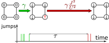
Figure 3: Top: Sketch of a possible relaxation trajectory for an initially empty (left) four-site Fermi-Hubbard model at zero temperature. After a quick relaxation process the system may reach e.g. the state $\left|{\mathord{\downarrow}}{\mathord{\downarrow}}{\mathord{\uparrow}}{\mathord{\downarrow}}\right>$, which is inert to the local dissipation, but due to the ${\mathord{\uparrow}}$-spin (marked red) is not yet a steady state. The internal dynamics of the Hamiltonian in combination with dissipation then finally admits to reach one of the steady states at much longer timescales. Bottom: The statistics between quantum jumps can reveal information on the involved timescales.

While the Mott insulator property at half filling remains stable after coupling to the reservoir (provided that it has an intermediate chemical potential), we found that dissipation tends to destroy the anti-ferromagnetic order of the Mott-Néel state (which is the ground state in bi-partite lattices), even at zero temperature. The coupling to the reservoir tends to increase the total angular momentum $\langle\hat{\mbox{\boldmath$S$}}^{2}\rangle$, such that states with maximum $\langle\hat{\mbox{\boldmath$S$}}^{2}\rangle$ like the ferromagnetic state $|{\mathord{\uparrow}}{\mathord{\uparrow}}\dots\mathord{\uparrow}{\mathord{\uparrow}}\rangle$ are steady states. As an intuitive picture, the intra-system tunnel coupling $J$ induces an effective anti-ferromagnetic interaction between neighboring sites while the coupling to the (unpolarized) reservoir tends to “wash out” this ordering until an inert state (such as $|{\mathord{\uparrow}}{\mathord{\uparrow}}\dots\mathord{\uparrow}{\mathord{\uparrow}}\rangle$) is reached. In the regime that we considered, where local dissipators are valid, the Hubbard model ground state is not a steady state, even at vanishing temperatures. This is not too surprising as proving the existence of thermal system steady states typically requires non-local dissipators.

Let us discuss potential experimental realizations. In non-equilibrium settings, the waiting time distributions are experimentally accessible observables. For example, for the Fermi-Hubbard trimer with a built-in charge detector realized in Ref. hensgens2017a , extraction of the waiting time distribution requires time-resolved current measurements that have with very high accuracy been performed for simpler systems gustavsson2006a ; fujisawa2006a ; flindt2009a ; kurzmann2019a ; kleinherbers2021b . For larger systems, the relaxation time scales could be obtained by pump-probe schemes, e.g., in the 1T-$\rm TaS_{2}$ system. Even in equilibrium, the reservoir-induced suppression of the anti-ferromagnetic order (expected for the closed Fermi-Hubbard system on a bi-partite lattice) could be an experimentally observable signature. Note, however, that this anti-ferromagnetic order could also be enhanced or suppressed by other effects (such as direct magnetic interactions) which are not captured by the Fermi-Hubbard Hamiltonian considered here. As another point, several systems (such as 1T-$\rm TaS_{2}$) do not correspond to bi-partite lattices (e.g., an effectively triangular lattice structure). Nevertheless, even in the absence of perfect long-range anti-ferromagnetic order (as expected for bi-partite lattices), the closed Fermi-Hubbard system would still induce some (short-ranged or direction-dependent) anti-ferromagnetic correlations. On the other hand, the steady states with maximum $\langle\hat{\mbox{\boldmath$S$}}^{2}\rangle$ can be generated by $\hat{S}_{-}^{n}|{\mathord{\uparrow}}{\mathord{\uparrow}}\dots\mathord{\uparrow}{\mathord{\uparrow}}\rangle$ and are thus permutation invariant, which means that they do not have such anti-ferromagnetic correlations. As a result, one would expect that the impact of the environment tends to suppress these anti-ferromagnetic correlations also for triangular lattices – provided that the local Lindblad master equation used here yields a good approximation.

As an outlook, it should be interesting to study generalizations of this master equation by making it non-local in time and/or space, or by taking into account coherent tunneling processes, see also Refs. hofer2017a ; kleinherbers2020a ; wu2019b ; bertini2021a ; trushechkin2021a . The coherences should, however, play no crucial role in the regime where $J\ll\gamma$ as their generation due to the interdot tunneling ($\sim J$) is suppressed here. In contrast, for weak reservoir coupling $\gamma$ one should expect that the anti-ferromagnetic order remains stable due to the non-local system dynamics reflected in global Lindblad operators. For such Lindblad operators, it is well-known that generically the grand-canonical equilibrium state of the system is a stationary state. At sufficiently low temperatures, with chemical potentials chosen such that the system is half-filled, we thus expect the system to relax into the ground state of that sector (with anti-ferromagnetic order). The calculation of waiting time distributions can also exploit the block structure of $\hat{H}_{\rm eff}$ in this case. However, in contrast to the local case discussed here, energetically degenerate eigenstates will then form the blocks of $\hat{H}_{\rm eff}$. A bosonic reservoir (e.g., representing electron-phonon interactions brandes2005a ; queisser2019a ) in addition to the fermionic bath considered here could also alter our results (especially at finite temperatures) and introduce new time scales. In particular, these further interactions need in general not respect the block structure of $\hat{H}_{\rm eff}$. However, in the particular case that the interactions couple a generic reservoir operator $\hat{B}$ globally e.g. to the total on-site energy ($\hat{H}_{I}=\hat{H}_{\epsilon}\otimes\hat{B}$) or the total kinetic term ($\hat{H}_{I}=\hat{H}_{J}\otimes\hat{B}$) of the Hubbard model (I), they will preserve the same quantum numbers as the isolated system. Then, we expect just additional diagonal contributions to $\hat{H}_{\rm eff}$ and the same block structure. Beyond these considerations, it should be illuminating to explore the transition between the weak and strong system–bath coupling in the context of our results. Also non-locality in time or time-dependence of the Lindblad operators should provide additional insight into the system dynamics at intermediate times and is subject of our further research.

VIII Acknowledgments

This work was funded by the Deutsche Forschungsgemeinschaft (DFG, German Research Foundation) – Project-ID 278162697 – SFB 1242. The authors thank E. Kleinherbers and L. Litzba for discussions and valuable feedback on the manuscript.

Appendix A Microscopic derivation of local dissipators

In addition to the system Hamiltonian (I) we consider a tunnel coupling

$$\hat{H}_{I}=\sum_{\mu}\sum_{s}\sum_{k}\left[t_{\mu ks}\hat{c}_{\mu s}^{\dagger}\hat{c}_{\mu ks}+{\rm H.c.}\right]$$ (46)

with small tunnel amplitudes $t_{\mu ks}$ describing the tunneling of electrons of spin $s$ between site $\mu\in\{1,2,3,4\}$ and mode $k$ of the adjacent lead. The reservoirs are modeled as non-interacting fermions

$$\hat{H}_{B}=\sum_{\mu}\sum_{s}\sum_{k}\epsilon_{\mu ks}\hat{c}_{\mu ks}^{\dagger}\hat{c}_{\mu ks}\,,$$ (47)

where $\hat{c}_{\mu ks}^{\dagger}$ creates an electron of spin $s$ in mode $k$ of the reservoir attached to site $\mu$ with energy $\epsilon_{\mu ks}$. Usual derivations of master equations now employ a perturbative treatment in $\hat{H}_{I}$ (i.e., $\lambda$) only breuer2002 . We are however interested in the regime where $J$ is smaller than the $t_{\mu ks}$, such that we follow a slightly different derivation where system-reservoir ($t_{\mu ks}$) and intra-system ($J$) tunnel couplings are treated on the same footing. Following Ref. landi2021a , we split the Hubbard Hamiltonian (I) as $\hat{H}=\hat{H}_{0}+\hat{H}_{J}$ with $\hat{H}_{0}=\hat{H}_{\epsilon}+\hat{H}_{U}$. With this, we can go to an interaction picture with respect to the free Hamiltonian of system and reservoir $\hat{H}_{0}+\hat{H}_{B}$ within which the operators follow the time-dependence

$$\hat{\mbox{\boldmath$c$}}_{\mu ks}(t) =e^{-\mathrm{i}\epsilon_{\mu ks}t}\hat{c}_{\mu ks}\,,$$

$$\hat{\mbox{\boldmath$c$}}_{\mu s}(t) =e^{-\mathrm{i}\epsilon t}(1-\hat{n}_{i}^{\bar{s}})\hat{c}_{\mu s}+e^{-\mathrm{i}(\epsilon+U)t}\hat{n}_{\mu}^{\bar{s}}\hat{c}_{\mu s}$$ (48)

and analogous for the creation operators – we use bold symbols to mark the interaction picture. In this interaction picture, the density matrix of the universe follows the von-Neumann equation

$$\frac{d}{dt}\hat{\mbox{\boldmath$\rho$}}_{\rm tot}=-\mathrm{i}\left[\hat{\mbox{\boldmath$H$}}_{J}(t),\hat{\mbox{\boldmath$\rho$}}_{\rm tot}(t)\right]-\mathrm{i}\left[\hat{\mbox{\boldmath$H$}}_{I}(t),\hat{\mbox{\boldmath$\rho$}}_{\rm tot}(t)\right]\,.$$ (49)

We formally integrate the above equation, but – in contrast to standard derivations – insert the solution only in the second term of the r.h.s. Performing a partial trace over the reservoir $\hat{\mbox{\boldmath$\rho$}}(t)={\rm Tr_{B}}\left\{\hat{\mbox{\boldmath$\rho$}}_{\rm tot}(t)\right\}$ then yields

$$\frac{d}{dt}\hat{\mbox{\boldmath$\rho$}} =-\mathrm{i}\left[\hat{\mbox{\boldmath$H$}}_{J}(t),{\rm Tr_{B}}\left\{\hat{\mbox{\boldmath$\rho$}}_{\rm tot}(t)\right\}\right]-\mathrm{i}{\rm Tr_{B}}\left\{\left[\hat{\mbox{\boldmath$H$}}_{I}(t),\hat{\rho}_{0}\right]\right\}$$

$$\;\;-\int\limits_{0}^{t}{\rm Tr_{B}}\left\{\left[\hat{\mbox{\boldmath$H$}}_{I}(t),\left[\hat{\mbox{\boldmath$H$}}_{J}(t^{\prime})+\hat{\mbox{\boldmath$H$}}_{I}(t^{\prime}),\mbox{\boldmath$\rho$}_{\rm tot}(t^{\prime})\right]\right]\right\}dt^{\prime}\,.$$ (50)

This equation is still exact but untreatable. We therefore employ the Born approximation at all times

$$\hat{\mbox{\boldmath$\rho$}}_{\rm tot}(t)=\hat{\mbox{\boldmath$\rho$}}(t)\otimes\hat{\rho}_{B}+{\cal O}\{t_{\mu ks}\}+{\cal O}\{J\}\,,$$ (51)

with $\hat{\rho}_{B}$ denoting the grand-canonical Gibbs state of the four leads, and where the corrections result from the fact that system-reservoir correlations are neglected and that also $\hat{\mbox{\boldmath$\rho$}}(t)$ only represents an approximation to the exact reduced density matrix of the system. Inserting it on the r.h.s., we obtain a closed but non-Markovian master equation for the system density matrix only

$$\frac{d}{dt}\hat{\mbox{\boldmath$\rho$}} =-\mathrm{i}\left[\hat{\mbox{\boldmath$H$}}_{J}(t),\hat{\mbox{\boldmath$\rho$}}(t)\right]$$

$$\qquad-\int\limits_{0}^{t}{\rm Tr_{B}}\left\{\left[\hat{\mbox{\boldmath$H$}}_{I}(t),\left[\hat{\mbox{\boldmath$H$}}_{I}(t^{\prime}),\hat{\mbox{\boldmath$\rho$}}(t^{\prime})\otimes\hat{\rho}_{B}\right]\right]\right\}dt^{\prime}$$

$$\qquad+{\cal O}\{J^{2},t_{\mu ks}J\}+{\cal O}\{t_{\mu ks}^{3},t_{\mu ks}^{2}J,t_{\mu ks}J^{2}\}\,.$$ (52)

Here, we have used the following: First, the first commutator term in (A) generates corrections of order $J^{2}$ and $Jt_{\mu ks}$, since $\hat{\mbox{\boldmath$\rho$}}$ is only an approximation to the exact reduced density matrix ${\rm Tr_{B}}\left\{\hat{\mbox{\boldmath$\rho$}}_{\rm tot}\right\}$. Second, for a reservoir in the Gibbs state and linear couplings we have ${\rm Tr_{B}}\left\{\hat{\mbox{\boldmath$H$}}_{I}(t)\hat{\rho}_{B}\right\}=\hat{0}$, such that the second commutator term in (A) vanishes exactly. Third, under the same reasoning the mixed double commutator term involving both $\hat{\mbox{\boldmath$H$}}_{I}$ and $\hat{\mbox{\boldmath$H$}}_{J}$ generates terms of ${\cal O}\{t_{\mu ks}^{2}J,t_{\mu ks}J^{2}\}$ and the double commutator term involving $\hat{\mbox{\boldmath$H$}}_{I}$ twice with the correction to the Born-approximated density matrix generates terms of ${\cal O}\{t_{\mu ks}^{2}J,t_{\mu ks}^{3}\}$. Using additionally that $\hat{H}_{I}=\sum_{\mu s}\hat{H}_{I}^{\mu s}$ with $\hat{H}_{I}^{\mu s}=\hat{c}_{\mu s}^{\dagger}\sum_{k}t_{\mu ks}\hat{c}_{\mu ks}+{\rm H.c.}$ and that $\hat{\rho}_{B}=\bigotimes_{\mu s}\hat{\rho}_{B}^{\mu s}$ with grand-canonical Gibbs state $\hat{\rho}_{B}^{\mu s}$ of the spin $s$ population in the $\mu$th lead, we can analogously use the property ${\rm Tr_{\mu s}}\left\{\hat{\mbox{\boldmath$H$}}_{I}^{\mu s}(t)\hat{\rho}_{B}^{\mu s}\right\}=0$ to further conclude

$$\frac{d}{dt}\hat{\mbox{\boldmath$\rho$}} =-\mathrm{i}\left[\hat{\mbox{\boldmath$H$}}_{J}(t),\hat{\mbox{\boldmath$\rho$}}(t)\right]$$

$$\;\;-\sum_{\mu s}\int\limits_{0}^{t}{\rm Tr_{\mu s}}\left\{\left[\hat{\mbox{\boldmath$H$}}_{I}^{\mu s}(t),\left[\hat{\mbox{\boldmath$H$}}_{I}^{\mu s}(t^{\prime}),\hat{\mbox{\boldmath$\rho$}}(t^{\prime})\otimes\hat{\rho}_{B}^{\mu s}\right]\right]\right\}dt^{\prime}$$

$$\;\;+{\cal O}\{J^{2},t_{\mu ks}J\}+{\cal O}\{t_{\mu ks}^{3},t_{\mu ks}^{2}J,t_{\mu ks}J^{2}\}\,.$$ (53)

Hence, if ${\cal O}\{J\}\leq{\cal O}\{t_{\mu ks}^{2}\}$, the above equation is still second-order accurate in the system-reservoir coupling strength. An important observation is now that the dissipator originating from the second line only is identical to the one that one would obtain if the sites of the Hubbard model were via $\hat{\mbox{\boldmath$H$}}_{I}^{\mu s}$ exclusively coupled to their local reservoir (as if one would consider the limit $J\to 0$).

We further proceed as it is standard practice: First, we express the partial trace by introducing correlation functions whose fast decay is then used to motivate the Markov approximations $\hat{\mbox{\boldmath$\rho$}}(t^{\prime})\to\hat{\mbox{\boldmath$\rho$}}(t)$ and $\int_{0}^{t}dt^{\prime}\to\int_{0}^{\infty}dt^{\prime}$. Second, we perform the secular approximation with respect to the energy scales of $\hat{H}_{0}$ only (note that the degeneracy of the states ${\mathord{\uparrow}}$ and ${\mathord{\downarrow}}$ on the same site is unproblematic here as we have already separated the spin species). Finally, we transform back to the Schrödinger picture, where $\hat{H}_{J}$ and $\hat{H}_{0}$ recombine to the original system Hamiltonian. Details for a single dot are presented in App. E. It should be noted here that the secular approximation is not the only possibility and more sophisticated methods, such as the coherent approximation kleinherbers2020a , are available at this step. However, the coherences are not expected to play a crucial role in the regime of small $J$. Their generation is related to the weak interdot tunneling ($\sim J$) and hence is supposed to give rise to small corrections only.

The net result of this procedure is a dissipator (excluding the Hamiltonian) that is additively composed from the local dissipators that one would have obtained if the sites of the model were exclusively coupled to their adjacent reservoir (see e.g. Ref. souza2007a for a single dot master equation). Thus, in this limit the only coupling between the sites is mediated by the Fermi-Hubbard Hamiltonian. Furthermore assuming that the spectral densities are frequency independent (wideband limit) $\Gamma_{\mu s}(\omega)=2\pi\sum_{k}{\left|t_{\mu ks}\right|}^{2}\delta(\omega-\epsilon_{\mu ks})=\gamma$ and identical for sites and spins, we precisely obtain an LGKS generator (2) with Hamiltonian (I) and Lindblad operators (VI) as outlined in the main text that is valid up to first order in $\gamma$ in the regime where $J<\gamma$.

Appendix B Quasimomentum in ring-shaped Fermi-Hubbard models

When the lattice structure of (I) is one-dimensional and periodic, i.e, ring-shaped, we can employ a one-dimensional discrete Fourier transform

$$\hat{c}_{\mu s}=\frac{1}{\sqrt{M}}\sum_{k=1}^{M}\hat{c}_{ks}e^{-2\pi\mathrm{i}\mu k/M}$$ (54)

to new fermionic operators $\hat{c}_{ks}$, where $M$ denotes the number of lattice sites. This transforms the Hamiltonian into

$$\hat{H} =\sum_{k=1}^{M}\sum_{s}\left[\epsilon-2J\cos\left(\frac{2\pi k}{M}\right)\right]\hat{c}_{ks}^{\dagger}\hat{c}_{ks}$$ (55)

$$+\frac{U}{M}\sum_{kk^{\prime}qq^{\prime}}\left[\sum_{j=1}^{M}\frac{e^{+2\pi\mathrm{i}j(k-k^{\prime}+q-q^{\prime})/M}}{M}\right]\hat{c}_{k{\mathord{\uparrow}}}^{\dagger}\hat{c}_{k^{\prime}{\mathord{\uparrow}}}\hat{c}_{q{\mathord{\downarrow}}}^{\dagger}\hat{c}_{q^{\prime}{\mathord{\downarrow}}}\,,$$

where the quadratic part is already diagonal but the Coulomb interaction looks like a scattering process. The square bracket in front of the scattering term ensures that $k+q=k^{\prime}+q^{\prime}$ is conserved modulo $M$. This periodicity of the exponential function together with the fact that e.g. for the tetramer we have $(k-k^{\prime}+q-q^{\prime})\in\{-6,\ldots,+6\}$ leads to a subtle definition of a conserved quasi-momentum operator. For example, the operator

$$\hat{Q} =\sum_{k=1}^{M}\sum_{s}k\hat{c}_{ks}^{\dagger}\hat{c}_{ks}$$ (56)

is not conserved essler2005 . However, the projectors onto sub-spaces of its eigenvalues modulo $M$

$$\hat{P}_{q} =\frac{1}{M}\sum_{j=1}^{M}\exp\left\{2\pi\mathrm{i}\frac{j}{M}\left(\hat{Q}-q\cdot\mbox{\boldmath$1$}\right)\right\}$$ (57)

are conserved $[\hat{H},\hat{P}_{q}]=0$, which allows one to define a quasi-momentum in various ways. For example, we could use these projectors to define the quasi-momentum as $\hat{P}=\sum_{q=1}^{M}q\cdot\hat{P}_{q}$. Alternatively, we could use the definition

$$\hat{P}=-\mathrm{i}\frac{M}{2\pi}\ln e^{\frac{2\pi\mathrm{i}}{M}\hat{Q}}\,.$$ (58)

In any case, the quasi-momentum operator is now conserved under the isolated Hubbard (I) dynamics $[\hat{H},\hat{P}]=0$.

The quasimomentum generates rotations which can actually be seen from

$$\hat{P}_{1234}\hat{c}_{\mu s}\hat{P}_{1234} =e^{+\frac{2\pi\mathrm{i}}{M}\hat{P}}\hat{c}_{\mu s}e^{-\frac{2\pi\mathrm{i}}{M}\hat{P}}$$

$$=e^{+\frac{2\pi\mathrm{i}}{M}\hat{Q}}\hat{c}_{\mu s}e^{-\frac{2\pi\mathrm{i}}{M}\hat{Q}}$$

$$=\frac{1}{\sqrt{M}}\sum_{k}e^{-\frac{2\pi\mathrm{i}\mu k}{M}}e^{+\frac{2\pi\mathrm{i}k}{M}\hat{c}_{ks}^{\dagger}\hat{c}_{ks}}\hat{c}_{ks}e^{-\frac{2\pi\mathrm{i}k}{M}\hat{c}_{ks}^{\dagger}\hat{c}_{ks}}$$

$$=\frac{1}{\sqrt{M}}\sum_{k}e^{-\frac{2\pi\mathrm{i}\mu k}{M}}e^{-\frac{2\pi\mathrm{i}k}{M}}\hat{c}_{ks}$$

$$=\hat{c}_{\mu+1,s}\,.$$ (59)

For the tetramer, each of the four quasi-momentum sectors hosts $64$ states.

Appendix C Heisenberg limit

In the isolated case $\gamma=0$, we can compare the lowest-lying of our approximate eigenvalues (27) and (V) with the effective Heisenberg Hamiltonian, that arises for large Coulomb repulsion. For $\epsilon=0$ it reads in the sub-space of absent doublon-holon occupations cleveland1976a

$$\hat{H}_{\rm Heis} =\sum_{\langle\mu,\nu\rangle}\frac{J^{2}}{U}\left[2\hat{\mbox{\boldmath$S$}}_{\mu}\cdot\hat{\mbox{\boldmath$S$}}_{\nu}-\frac{1}{2}\right]$$

$$=\sum_{\mu}\frac{J^{2}}{U}\left[4\hat{\mbox{\boldmath$S$}}_{\mu}\cdot\hat{\mbox{\boldmath$S$}}_{\mu+1}-1\right]\,,$$ (60)

where we have resolved the double-counting in the second line. Computing the expectation value of this Hamiltonian in the ground state of (32), we obtain by virtue of $\left<-\sum_{\mu}\hat{\mbox{\boldmath$S$}}_{\mu}\cdot\hat{\mbox{\boldmath$S$}}_{\mu+1}\right>\approx 2$ for the tetramer

$$\left<\hat{H}_{\rm Heis}\right>\approx-12\frac{J^{2}}{U}\,,$$ (61)

which – together with the on-site energy of $4\epsilon$ – provides the first eigenvalue of (V) for $\gamma=0$. Analogously, doing the same for the ground state of (26), for which we have $\left<-\sum_{\mu}\hat{\mbox{\boldmath$S$}}_{\mu}\cdot\hat{\mbox{\boldmath$S$}}_{\mu+1}\right>\approx 1$, we obtain

$$\left<\hat{H}_{\rm Heis}\right>\approx-8\frac{J^{2}}{U}\,,$$ (62)

which (taking again the on-site energy shift of $4\epsilon$ into account) provides the first eigenvalue of (27) for $\gamma=0$.

Appendix D Decay characteristics of other states in the Fermi-Hubbard tetramer

In the sub-space with $N=4$ and $S_{z}=0$ ($N_{\mathord{\uparrow}}=N_{\mathord{\downarrow}}=2$) containing 36 states, the effective non-Hermitian Hamiltonian can be decomposed into 4 blocks of size $1\times 1$, 10 blocks of size $2\times 2$, and 4 blocks of size $3\times 3$ with different quantum numbers of $\hat{\mbox{\boldmath$S$}}^{2}$, $\hat{\eta}^{2}$, and quasi-momentum $\hat{P}$. The eigenvalues of each of these blocks can be analytically evaluated as we did in the main text. In the zero-temperature limit, this leads to the qualitative decay chart provided in Fig. 4.

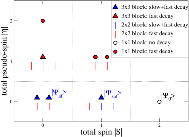
Figure 4: Qualitative classification of the decay dynamics of states in the $N_{\mathord{\uparrow}}=N_{\mathord{\downarrow}}=2$ sector at zero temperature versus total spin ${\left|S\right|}\in\{0,1,2\}$ and pseudo-spin ${\left|\eta\right|}\in\{0,1,2\}$. Circles encode $1\times 1$ blocks, lines encode $2\times 2$ blocks and triangles encode $3\times 3$ blocks of the effective non-Hermitian Hamiltonian (each symbol is associated to a unique quasi-momentum value). For red symbols, the decay is always just fast, for the blue symbols we have a slow mode participating in the dynamics, and the hollow symbol corresponds to the quintuplett steady state of this sector. The two marked triangles correspond to Eqns. (32) and (26) and the marked circle to the $S_{z}=0$ state in (V) in the main text, respectively.

Blocks with non-vanishing pseudo-spin all decay trivially (red symbols), i.e., at least as fast as ${\cal O}\{\gamma\}$. Among the blocks with vanishing pseudo-spin, some decay non-trivially (blue symbols), i.e., one mode decays slower as ${\cal O}\{\gamma J^{2}/U^{2}\}$. It can thus be seen that states with a non-vanishing pseudo-spin always decay fast with timescale $\gamma$, in agreement with Eq. (III).

The sub-spaces of other particle numbers then also host blocks of size $4\times 4$ that decay fast (not shown).

Appendix E Markov and secular approximations for a single dot

For notational ease, we just consider the dissipator from (A) only for a single site, such that we can drop the site index $\mu$ (the treatment is identical for all sites). Then, it reads

$${\cal D}_{s}\hat{\mbox{\boldmath$\rho$}} =-\int_{0}^{t}{\rm Tr_{B}}\left\{\left[\hat{\mbox{\boldmath$H$}}_{I}^{s}(t),\left[\hat{\mbox{\boldmath$H$}}_{I}^{s}(t^{\prime}),\hat{\mbox{\boldmath$\rho$}}(t^{\prime})\otimes\hat{\rho}_{B}\right]\right]\right\}dt^{\prime}\,,$$ (63)

where the interaction Hamiltonian is given by $\hat{H}_{I}^{s}=\hat{c}_{s}^{\dagger}\hat{B}_{s}+{\rm H.c.}$ with $\hat{B}_{s}=\sum_{k}t_{ks}\hat{c}_{ks}$ denoting the reservoir coupling operator. Bold symbols denote our interaction picture with respect to $\hat{H}_{B}+\hat{H}_{\epsilon}+\hat{H}_{U}$, where we write (A) as $\hat{\mbox{\boldmath$c$}}_{ks}(t)=e^{-\mathrm{i}\epsilon_{ks}t}\hat{c}_{ks}$ and $\hat{\mbox{\boldmath$c$}}_{s}(t)=e^{-\mathrm{i}\epsilon t}\hat{c}_{s}(1-\hat{n}_{\bar{s}})+e^{-\mathrm{i}(\epsilon+U)t}\hat{c}_{s}\hat{n}_{\bar{s}}$ with bath mode energies $\epsilon_{ks}$.

The evaluation of the partial trace motivates to define the two non-vanishing reservoir correlation functions

$$C_{1}(\tau) ={\rm Tr_{B}}\left\{\hat{\mbox{\boldmath$B$}}_{s}(\tau)\hat{B}_{s}^{\dagger}\hat{\rho}_{B}\right\}=\int\frac{d\omega}{2\pi}\Gamma(\omega)[1-f(\omega)]e^{-\mathrm{i}\omega\tau}\,,$$

$$C_{2}(\tau) ={\rm Tr_{B}}\left\{\hat{\mbox{\boldmath$B$}}_{s}^{\dagger}(\tau)\hat{B}_{s}\hat{\rho}_{B}\right\}=\int\frac{d\omega}{2\pi}\Gamma(\omega)f(\omega)e^{+\mathrm{i}\omega\tau}\,,$$ (64)

where we have introduced the spectral coupling density $\Gamma(\omega)=2\pi\sum_{k}{\left|t_{ks}\right|}^{2}\delta(\omega-\epsilon_{ks})$ and $f(\omega)$ is the Fermi function of the reservoir. Since in our model neither of these depend on the spin, we have dropped its index in these quantities.

For rapidly decaying reservoir correlation functions (flat Fourier transforms) we can perform the usual Markov approximation on the dissipator

$${\cal D}_{s}\hat{\mbox{\boldmath$\rho$}} \approx-\int_{0}^{\infty}d\tau\Big{\{}\left[\hat{\mbox{\boldmath$c$}}_{s}^{\dagger}(t),\hat{\mbox{\boldmath$c$}}_{s}(t-\tau)\hat{\mbox{\boldmath$\rho$}}(t)\right]C_{1}(\tau)$$

$$\qquad+\left[\hat{\mbox{\boldmath$\rho$}}(t)\hat{\mbox{\boldmath$c$}}_{s}(t-\tau),\hat{\mbox{\boldmath$c$}}_{s}^{\dagger}(t)\right]C_{2}(-\tau)$$

$$\qquad+\left[\hat{\mbox{\boldmath$c$}}_{s}(t),\hat{\mbox{\boldmath$c$}}_{s}^{\dagger}(t-\tau)\hat{\mbox{\boldmath$\rho$}}(t)\right]C_{2}(\tau)$$

$$\qquad+\left[\hat{\mbox{\boldmath$\rho$}}(t)\hat{\mbox{\boldmath$c$}}_{s}^{\dagger}(t-\tau),\hat{\mbox{\boldmath$c$}}_{s}(t)\right]C_{1}(-\tau)\Big{\}}\,,$$ (65)

which is the (local) Redfield master equation.

In the subsequent secular approximation, we neglect terms that oscillate in time $t$ in the interaction picture. For large times $Ut\gg 1$, only few terms remain

$${\cal D}_{s}\hat{\mbox{\boldmath$\rho$}} \approx-\int_{0}^{\infty}d\tau\Big{\{}\left[\hat{c}_{s}^{\dagger}(1-\hat{n}_{\bar{s}}),\hat{c}_{s}(1-\hat{n}_{\bar{s}})\hat{\mbox{\boldmath$\rho$}}(t)\right]e^{+\mathrm{i}\epsilon\tau}C_{1}(\tau)$$

$$\qquad+\left[\hat{c}_{s}^{\dagger}\hat{n}_{\bar{s}},\hat{c}_{s}\hat{n}_{\bar{s}}\hat{\mbox{\boldmath$\rho$}}(t)\right]e^{+\mathrm{i}(\epsilon+U)\tau}C_{1}(\tau)$$

$$\qquad+\left[\hat{\mbox{\boldmath$\rho$}}(t)\hat{c}_{s}(1-\hat{n}_{\bar{s}}),\hat{c}_{s}^{\dagger}(1-\hat{n}_{\bar{s}})\right]e^{+\mathrm{i}\epsilon\tau}C_{2}(-\tau)$$

$$\qquad+\left[\hat{\mbox{\boldmath$\rho$}}(t)\hat{c}_{s}\hat{n}_{\bar{s}},\hat{c}_{s}^{\dagger}\hat{n}_{\bar{s}}\right]e^{+\mathrm{i}(\epsilon+U)\tau}C_{2}(-\tau)$$

$$\qquad+\left[\hat{c}_{s}(1-\hat{n}_{\bar{s}}),\hat{c}_{s}^{\dagger}(1-\hat{n}_{\bar{s}})\hat{\mbox{\boldmath$\rho$}}(t)\right]e^{-\mathrm{i}\epsilon\tau}C_{2}(\tau)$$

$$\qquad+\left[\hat{c}_{s}\hat{n}_{\bar{s}},\hat{c}_{s}^{\dagger}\hat{n}_{\bar{s}}\hat{\mbox{\boldmath$\rho$}}(t)\right]e^{-\mathrm{i}(\epsilon+U)\tau}C_{2}(\tau)$$

$$\qquad+\left[\hat{\mbox{\boldmath$\rho$}}(t)\hat{c}_{s}^{\dagger}(1-\hat{n}_{\bar{s}}),\hat{c}_{s}(1-\hat{n}_{\bar{s}})\right]e^{-\mathrm{i}\epsilon\tau}C_{1}(-\tau)$$

$$\qquad+\left[\hat{\mbox{\boldmath$\rho$}}(t)\hat{c}_{s}^{\dagger}\hat{n}_{\bar{s}},\hat{c}_{s}\hat{n}_{\bar{s}}\right]e^{-\mathrm{i}(\epsilon+U)\tau}C_{1}(-\tau)\Big{\}}\,.$$ (66)

To get rid of the remaining integration we insert the Fourier decomposition (E) of the correlation functions and then use the Sokhotski-Plemelj theorem

$$\frac{1}{2\pi}\int_{0}^{\infty}e^{+\mathrm{i}\omega\tau}d\tau=\frac{1}{2}\delta(\omega)+\frac{\mathrm{i}}{2\pi}{\cal P}\frac{1}{\omega}\,.$$ (67)

Here, the first term is relevant and the second eventually yields the Lamb-shift terms (which can be absorbed in renormalized onsite energies $\epsilon$ and Coulomb interaction $U$ such that we neglect them here). This yields

$${\cal D}_{s}\hat{\mbox{\boldmath$\rho$}} \approx\gamma(1-f_{\rm E})\Big{[}\hat{c}_{s}(1-\hat{n}_{\bar{s}})\hat{\mbox{\boldmath$\rho$}}(t)\hat{c}_{s}^{\dagger}(1-\hat{n}_{\bar{s}})$$

$$\qquad\qquad-\frac{1}{2}\left\{\hat{n}_{s}(1-\hat{n}_{\bar{s}})^{2},\hat{\mbox{\boldmath$\rho$}}(t)\right\}\Big{]}$$

$$\qquad+\gamma(1-f_{\rm U})\left[\hat{c}_{s}\hat{n}_{\bar{s}}\hat{\mbox{\boldmath$\rho$}}(t)\hat{c}_{s}^{\dagger}\hat{n}_{\bar{s}}-\frac{1}{2}\left\{\hat{n}_{s}\hat{n}_{\bar{s}}^{2},\hat{\mbox{\boldmath$\rho$}}(t)\right\}\right]$$

$$\qquad+\gamma f_{\rm E}\Big{[}\hat{c}_{s}^{\dagger}(1-\hat{n}_{\bar{s}})\hat{\mbox{\boldmath$\rho$}}(t)\hat{c}_{s}(1-\hat{n}_{\bar{s}})$$

$$\qquad\qquad-\frac{1}{2}\left\{(1-\hat{n}_{s})(1-\hat{n}_{\bar{s}})^{2},\hat{\mbox{\boldmath$\rho$}}(t)\right\}\Big{]}$$

$$\qquad+\gamma f_{\rm U}\left[\hat{c}_{s}^{\dagger}\hat{n}_{\bar{s}}\hat{\mbox{\boldmath$\rho$}}(t)\hat{c}_{s}\hat{n}_{\bar{s}}-\frac{1}{2}\left\{\hat{c}_{s}\hat{c}_{s}^{\dagger}\hat{n}_{\bar{s}}^{2},\hat{\mbox{\boldmath$\rho$}}(t)\right\}\right]\,,$$ (68)

where we have assumed the wideband limit over the system energy scales $\Gamma(\epsilon)=\Gamma(\epsilon+U)=\gamma$ and abbreviated $f_{\rm E}=[e^{\beta(\epsilon-\mu_{\rm b})}+1]^{-1}$ and $f_{\rm U}=[e^{\beta(\epsilon+U-\mu_{\rm b})}+1]^{-1}$, compare (VI) in the main text. Under the transformation back to the Schrödinger picture, in the dissipator we only have to replace $\hat{\mbox{\boldmath$\rho$}}(t)\to\hat{\rho}(t)$.

Finally, we just note that it is not permissible to perform the limit $U\to 0$ a posteriori, as this conflicts with the secular approximation performed. Instead, in this limit an analogous derivation with $\hat{\mbox{\boldmath$c$}}_{s}(t)=e^{-\mathrm{i}\epsilon t}\hat{c}_{s}$ has to be followed, which would yield a Lindblad dissipator where the different spin-species do not interact

$${\cal D}_{s}^{U=0}\hat{\mbox{\boldmath$\rho$}} \approx\gamma(1-f)\left[\hat{c}_{s}\hat{\mbox{\boldmath$\rho$}}(t)\hat{c}_{s}^{\dagger}-\frac{1}{2}\left\{\hat{c}_{s}^{\dagger}\hat{c}_{s},\hat{\mbox{\boldmath$\rho$}}(t)\right\}\right]$$

$$\qquad+\gamma f\left[\hat{c}_{s}^{\dagger}\hat{\mbox{\boldmath$\rho$}}(t)\hat{c}_{s}-\frac{1}{2}\left\{\hat{c}_{s}\hat{c}_{s}^{\dagger},\hat{\mbox{\boldmath$\rho$}}(t)\right\}\right]\,.$$ (69)

References

- (1) C. Kollath, A. M. Läuchli, and E. Altman. Quench dynamics and nonequilibrium phase diagram of the Bose-Hubbard model. Phys. Rev. Lett. 98, 180601 (2007).
- (2) M. Eckstein, M. Kollar, and P. Werner. Thermalization after an interaction quench in the Hubbard model. Phys. Rev. Lett. 103, 056403 (2009).
- (3) M. Moeckel and S. Kehrein. Interaction quench in the Hubbard model. Phys. Rev. Lett. 100, 175702 (2008).
- (4) S. Trotzky, Y.-A. Chen, A. Flesch, I. P. McCulloch, U. Schollwöck, J. Eisert, and I. Bloch. Probing the relaxation towards equilibrium in an isolated strongly correlated one-dimensional Bose gas. Nature Physics 8, 325 (2012).
- (5) H. Bruus and K. Flensberg. Many-body quantum theory incondensed matter physics. Oxford University Press, Oxford, Oxford graduate texts edn. (2002).
- (6) D. Lacroix, S. Hermanns, C. M. Hinz, and M. Bonitz. Ultrafast dynamics of finite Hubbard clusters: A stochastic mean-field approach. Phys. Rev. B 90, 125112 (2014).
- (7) M. Imada, A. Fujimori, and Y. Tokura. Metal-insulator transitions. Rev. Mod. Phys. 70, 1039 (1998).
- (8) E. H. Lieb. The Hubbard model: Some Rigorous Results and Open Problems, 59–77. Springer Berlin Heidelberg, Berlin, Heidelberg (2004). ISBN 978-3-662-06390-3.
- (9) F. H. L. Essler, H. Frahm, F. Gohmann, A. Klumper, and V. E. Korepin. The One-Dimensional Hubbard Model. Cambridge University Press, Cambridge (2005).
- (10) B. Edegger, V. N. Muthukumar, and C. Gros. Gutzwiller-RVB theory of high-temperature superconductivity: Results from renormalized mean-field theory and variational Monte Carlo calculations. Advances in Physics 56, 927 (2007).
- (11) T. Prosen. Exact nonequilibrium steady state of an open Hubbard chain. Phys. Rev. Lett. 112, 030603 (2014).
- (12) M. Nakagawa, N. Kawakami, and M. Ueda. Exact Liouvillian spectrum of a one-dimensional dissipative Hubbard model. Phys. Rev. Lett. 126, 110404 (2021).
- (13) B. Bertini, F. Heidrich-Meisner, C. Karrasch, T. Prosen, R. Steinigeweg, and M. Žnidarič. Finite-temperature transport in one-dimensional quantum lattice models. Rev. Mod. Phys. 93, 025003 (2021).
- (14) M. G. Priestley and D. Shoenberg. An experimental study of the Fermi surface of magnesium. Proceedings of the Royal Society of London. Series A. Mathematical and Physical Sciences 276, 258 (1963).
- (15) H. Tasaki. The Hubbard model - an introduction and selected rigorous results. Journal of Physics: Condensed Matter 10, 4353 (1998).
- (16) D. Jaksch and P. Zoller. The cold atom Hubbard toolbox. Annals of Physics 315, 52 (2005). ISSN 0003-4916. Special Issue.
- (17) T. Schäfer, F. Geles, D. Rost, G. Rohringer, E. Arrigoni, K. Held, N. Blümer, M. Aichhorn, and A. Toschi. Fate of the false Mott-Hubbard transition in two dimensions. Phys. Rev. B 91, 125109 (2015).
- (18) C. L. Cleveland and R. Medina A. Obtaining a Heisenberg Hamiltonian from the Hubbard model. American Journal of Physics 44, 44 (1976).
- (19) A. Klein and D. Jaksch. Simulating high-temperature superconductivity model Hamiltonians with atoms in optical lattices. Phys. Rev. A 73, 053613 (2006).
- (20) M. Qin, C.-M. Chung, H. Shi, E. Vitali, C. Hubig, U. Schollwöck, S. R. White, and S. Zhang. Absence of superconductivity in the pure two-dimensional Hubbard model. Phys. Rev. X 10, 031016 (2020).
- (21) W. Hofstetter, J. I. Cirac, P. Zoller, E. Demler, and M. D. Lukin. High-temperature superfluidity of fermionic atoms in optical lattices. Phys. Rev. Lett. 89, 220407 (2002).
- (22) W. V. Liu, F. Wilczek, and P. Zoller. Spin-dependent Hubbard model and a quantum phase transition in cold atoms. Phys. Rev. A 70, 033603 (2004).
- (23) T. Esslinger. Fermi-Hubbard physics with atoms in an optical lattice. Annual Review of Condensed Matter Physics 1, 129 (2010).
- (24) R. A. Hart, P. M. Duarte, T.-L. Yang, X. Liu, T. Paiva, E. Khatami, R. T. Scalettar, N. Trivedi, D. A. Huse, and R. G. Hulet. Observation of antiferromagnetic correlations in the Hubbard model with ultracold atoms. Nature 519, 211 (2015).
- (25) R. J. Hamers. Characterization of localized atomic surface defects by tunneling microscopy and spectroscopy. Journal of Vacuum Science & Technology B: Microelectronics Processing and Phenomena 6, 1462 (1988).
- (26) J. Salfi, J. A. Mol, R. Rahman, G. Klimeck, M. Y. Simmons, L. C. L. Hollenberg, and S. Rogge. Quantum simulation of the Hubbard model with dopant atoms in silicon. Nature Communications 7, 11342 (2016).
- (27) T. Hensgens, T. Fujita, L. Janssen, X. Li, C. J. V. Diepen, C. Reichl, W. Wegscheider, S. D. Sarma, and L. M. K. Vandersypen. Quantum simulation of a Fermi-Hubbard model using a semiconductor quantum dot array. Nature 548, 70 (2017).
- (28) U. Mukhopadhyay, J. P. Dehollain, C. Reichl, W. Wegscheider, and L. M. K. Vandersypen. A 2x2 quantum dot array with controllable inter-dot tunnel couplings. Applied Physics Letters 112, 183505 (2018).
- (29) R. Manzke, T. Buslaps, B. Pfalzgraf, M. Skibowski, and O. Anderson. On the phase transitions in 1 t -TaS 2. Europhysics Letters (EPL) 8, 195 (1989).
- (30) K. T. Law and P. A. Lee. as a quantum spin liquid. Proceedings of the National Academy of Sciences 114, 6996 (2017). ISSN 0027-8424.
- (31) I. Avigo, F. Queisser, P. Zhou, M. Ligges, K. Rossnagel, R. Schützhold, and U. Bovensiepen. Doublon bottleneck in the ultrafast relaxation dynamics of hot electrons in 1T-TaS2. Phys. Rev. Research 2, 022046 (2020).
- (32) T. Byrnes, P. Recher, N. Y. Kim, S. Utsunomiya, and Y. Yamamoto. Quantum simulator for the Hubbard model with long-range Coulomb interactions using surface acoustic waves. Physical Review Letters 99, 016405 (2007).
- (33) V. Gorini, A. Kossakowski, and E. C. G. Sudarshan. Completely positive dynamical semigroups of -level systems. Journal of Mathematical Physics 17, 821 (1976).
- (34) G. Lindblad. On the generators of quantum dynamical semigroups. Communications in Mathematical Physics 48, 119 (1976).
- (35) A. Carmele, M. Heyl, C. Kraus, and M. Dalmonte. Stretched exponential decay of Majorana edge modes in many-body localized Kitaev chains under dissipation. Phys. Rev. B 92, 195107 (2015).
- (36) V. Popkov and T. Prosen. Infinitely dimensional Lax structure for the one-dimensional Hubbard model. Phys. Rev. Lett. 114, 127201 (2015).
- (37) M. Žnidarič. Relaxation times of dissipative many-body quantum systems. Phys. Rev. E 92, 042143 (2015).
- (38) L.-N. Wu and A. Eckardt. Bath-induced decay of stark many-body localization. Phys. Rev. Lett. 123, 030602 (2019).
- (39) F. Queisser and R. Schützhold. Environment-induced prerelaxation in the Mott-Hubbard model. Phys. Rev. B 99, 155110 (2019).
- (40) E. Kleinherbers, N. Szpak, J. König, and R. Schützhold. Relaxation dynamics in a Hubbard dimer coupled to fermionic baths: Phenomenological description and its microscopic foundation. Phys. Rev. B 101, 125131 (2020).
- (41) Deviations from this assumption and the consequences of a global bath in comparison to local reservoirs will be discussed in a forthcoming publication.
- (42) H.-P. Breuer and F. Petruccione. The Theory of Open Quantum Systems. Oxford University Press, Oxford (2002).
- (43) E. H. Lieb. Two theorems on the Hubbard model. Phys. Rev. Lett. 62, 1201 (1989).
- (44) W.-H. Steeb, C. M. Villet, and P. Mulser. Hubbard model, conserved quantities,and computer algebra. International Journal of Theoretical Physics 32, 1445 (1993).
- (45) R. Schumann. Thermodynamics of a 4-site Hubbard model by analytical diagonalization. Annalen der Physik 11, 49 (2002).
- (46) A. Mielke. Many-Body Physics: From Kondo to Hubbard, chap. 11. The Hubbard Model and its Properties. Forschungszentrum Jülich, Jülich (2015). ISBN 978-3-95806-074-6.
- (47) C. N. Yang. pairing and off-diagonal long-range order in a Hubbard model. Phys. Rev. Lett. 63, 2144 (1989).
- (48) S. Zhang. Pseudospin symmetry and new collective modes of the Hubbard model. Phys. Rev. Lett. 65, 120 (1990).
- (49) V. V. Albert and L. Jiang. Symmetries and conserved quantities in Lindblad master equations. Phys. Rev. A 89, 022118 (2014).
- (50) D. Nigro. On the uniqueness of the steady-state solution of the Lindblad-Gorini-Kossakowski-Sudarshan equation. Journal of Statistical Mechanics: Theory and Experiment 2019, 043202 (2019).
- (51) F. Queisser, K. V. Krutitsky, P. Navez, and R. Schützhold. Equilibration and prethermalization in the Bose-Hubbard and Fermi-Hubbard models. Phys. Rev. A 89, 033616 (2014).
- (52) L.-N. Wu and A. Eckardt. Prethermal memory loss in interacting quantum systems coupled to thermal baths. Phys. Rev. B 101, 220302 (2020).
- (53) K. Wang, F. Piazza, and D. J. Luitz. Hierarchy of relaxation timescales in local random Liouvillians. Phys. Rev. Lett. 124, 100604 (2020).
- (54) C. Cohen-Tannoudji and J. Dalibar. Single-atom laser spectroscopy. Looking for dark periods in fluorescence light. Europhysics Letters 9, 441 (1986).
- (55) M. B. Plenio and P. L. Knight. The quantum-jump approach to dissipative dynamics in quantum optics. Rev. Mod. Phys. 70, 101 (1998).
- (56) T. Brandes. Waiting times and noise in single particle transport. Annalen der Physik (Berlin) 17, 477 (2008).
- (57) M. Albert, C. Flindt, and M. Büttiker. Distributions of waiting times of dynamic single-electron emitters. Phys. Rev. Lett. 107, 086805 (2011).
- (58) M. Albert, G. Haack, C. Flindt, and M. Büttiker. Electron waiting times in mesoscopic conductors. Phys. Rev. Lett. 108, 186806 (2012).
- (59) L. Rajabi, C. Pöltl, and M. Governale. Waiting time distributions for the transport through a quantum-dot tunnel coupled to one normal and one superconducting lead. Phys. Rev. Lett. 111, 067002 (2013).
- (60) B. Sothmann. Electronic waiting-time distribution of a quantum-dot spin valve. Phys. Rev. B 90, 155315 (2014).
- (61) K. Ptaszyński. Waiting time distribution revealing the internal spin dynamics in a double quantum dot. Phys. Rev. B 96, 035409 (2017).
- (62) E. Kleinherbers, P. Stegmann, and J. König. Synchronized coherent charge oscillations in coupled double quantum dots. Phys. Rev. B 104, 165304 (2021).
- (63) C. Buth, R. Santra, and L. S. Cederbaum. Non-Hermitian Rayleigh-Schrödinger perturbation theory. Phys. Rev. A 69, 032505 (2004).
- (64) Y. Ashida, Z. Gong, and M. Ueda. Non-hermitian physics. Advances in Physics 69, 249 (2020).
- (65) One actually finds in total four states with particles, , , and and odd parities , but one of these can be trivially decoupled. If one classifies the states by the more complicated quasi-momentum instead, the sector of interest contains only the three states discussed.
- (66) Acting with the hopping Hamiltonian on the state , we obtain the already orthogonal state . Acting again with the hopping Hamiltonian and orthogonalizing we obtain .
- (67) S. Gustavsson, R. Leturcq, B. Simovic, R. Schleser, T. Ihn, P. Studerus, K. Ensslin, D. C. Driscoll, and A. C. Gossard. Counting statistics of single electron transport in a quantum dot. Physical Review Letters 96, 076605 (2006).
- (68) T. Fujisawa, T. Hayashi, R. Tomita, and Y. Hirayama. Bidirectional counting of single electrons. Science 312, 1634 (2006).
- (69) C. Flindt, C. Fricke, F. Hohls, T. Novotny, K. Netocny, T. Brandes, and R. J. Haug. Universal oscillations in counting statistics. PNAS 106, 10116 (2009).
- (70) A. Kurzmann, P. Stegmann, J. Kerski, R. Schott, A. Ludwig, A. D. Wieck, J. König, A. Lorke, and M. Geller. Optical detection of single-electron tunneling into a semiconductor quantum dot. Phys. Rev. Lett. 122, 247403 (2019).
- (71) E. Kleinherbers, P. Stegmann, A. Kurzmann, M. Geller, A. Lorke, and J. König. Pushing the limits in real-time measurements of quantum dynamics. arXiv/2106.12502 (2021).
- (72) P. P. Hofer, M. Perarnau-Llobet, L. David, M. Miranda, G. Haack, R. Silva, J. B. Brask, and N. Brunner. Markovian master equations for quantum thermal machines: local versus global approach. New Journal of Physics 19, 123037 (2017).
- (73) L.-N. Wu, A. Schnell, G. D. Tomasi, M. Heyl, and A. Eckardt. Describing many-body localized systems in thermal environments. New Journal of Physics 21, 063026 (2019).
- (74) A. Trushechkin. Unified Gorini-Kossakowski-Lindblad-Sudarshan quantum master equation beyond the secular approximation. Phys. Rev. A 103, 062226 (2021).
- (75) T. Brandes. Coherent and collective quantum optical effects in mesoscopic systems. Physics Reports 408, 315 (2005).
- (76) G. Landi, D. Poletti, and G. Schaller. Non-equilibrium boundary driven quantum systems: models, methods and properties. arXiv:2104.14350 (2021).
- (77) F. M. Souza, J. C. Egues, and A. P. Jauho. Quantum dot as a spin-current diode: A master-equation approach. Phys. Rev. B 75, 165303 (2007).