DVHN: A Deep Hashing Framework for Large-scale Vehicle Re-identification

Abstract

Vehicle re-identification,  which seeks to match query vehicle images with tremendous gallery images , has been gathering proliferating momentum. Conventional methods generally perform re-identification tasks by representing vehicle images as real-valued feature vectors and then ranking the gallery images by computing the corresponding Euclidean distances. Despite achieving remarkable retrieval accuracy, these methods require tremendous memory and computation when the gallery set is large, making them inapplicable in real-world scenarios.

In light of this limitation, in this paper, we make the very first attempt to investigate the integration of deep hash learning with vehicle re-identification. We propose a deep hash-based vehicle re-identification framework, dubbed DVHN, which substantially reduces memory usage and promotes retrieval efficiency while reserving nearest neighbor search accuracy. Concretely, DVHN directly learns discrete compact binary hash codes for each image by jointly optimizing the feature learning network and the hash code generating module. Specifically, we directly constrain the output from the convolutional neural network to be discrete binary codes and ensure the learned binary codes are optimal for classification. To optimize the deep discrete hashing framework, we further propose an alternating minimization method for learning binary similarity-preserved hashing codes. Extensive experiments on two widely-studied vehicle re-identification datasets- VehicleID and VeRi- have demonstrated the superiority of our method against the state-of-the-art deep hash methods. DVHN of $2048$ bits can achieve 13.94% and 10.21% accuracy improvement in terms of mAP and Rank@1 for VehicleID (800) dataset. For VeRi, we achieve 35.45% and 32.72% performance gains for Rank@1 and mAP, respectively.

I Introduction

Vehicle re-identification (vehicle ReID)[1][2][3][4][5][6] has been receiving growing attention among the computer vision research community. It targets retrieving the corresponding vehicle images in the gallery set given a query image. The general re-identification framework consists of two module: feature learning and metric learning. 1) the feature learning module is responsible for extracting discriminative feature embedding from the vehicle image. 2) the distance metric learning module [7] is for preserving the distances of original images in the embedding space. Previous vehicle re-identification methods have achieved pronounced performances on widely-studied research datasets. Nonetheless, it is not feasible to apply these techniques directly into a real-world scenario where the gallery image set normally contains an astronomical amount of images. The main reasons are demonstrated as follows. First, since existing methods learns a real- valued feature vector for each image, the memory storage cost could be exceedingly high when there exists a large number of images. For instance, storing a 2048-dimensional feature vector of data type ‘float64’ takes up 16 kilobytes. For a gallery set of 10 million vehicle images, the total memory storage cost could be up to 150 gigabytes. On top of that, directly computing the similarity between two 2048-dimensional feature vectors is quite inefficient[8] and costly, making it undesirable when the query speed is a critical concern.

Recently, substantial research efforts have been devoted to deep learning-based hash methods owing to their low storage cost and high retrieval efficiency. The goal of deep hash is to learn a hash function that embeds images into compact binary hash codes in the hamming space while preserving their similarity in the original space[9][10][11][8]. Since a 2048-bit hamming code only takes up 256 bytes in memory, the total storage for a dataset of 10 million images is less than 2.4 gigabytes, saving up to 147 gigabytes of memory compared to using real-valued feature vectors. Further, as stated in [12], the computation of Hamming distance between binary hash codes can be accelerated by using the built-in CPU hardware instruction-XOR. Generally, the hamming distance computation could be completed with several machine instructions, significantly faster than computing its euclidean distance counterpart.

Captivated by the before-mentioned benefits, one may naturally ponder the possibility of directly applying the off-the-shelf deep hash techniques into addressing the large-scale vehicle ReID problem.  Although researchers have successfully applied deep hashing in the image retrieval, the unique features of the ReID task make it non-trivial to apply these methods directly, usually with notable performance drops. The degraded performance could be ascribed to the fact that general-purposed deep hash methods fail to learn robust and discriminative features of vehicle ReID datasets. For instance, canonical deep hash methods[11][13] adopt a convolutional neural network to learn features and a pairwise loss module to guide the generation of hamming code. In a scenario where there are thousands, even millions of vehicle ids, and where viewpoint variation for each vehicle identity is considerable, these off-the-shelf deep hash methods can only learn sub-optimal feature representation, leading to sub-optimal hash codes.

In this paper, we introduce a novel deep hash-based framework for efficient large-scale vehicle ReID, dubbed DVHN, which fully exploit the merits of deep hashing learning while preserving the retrieval accuracy in large-scale vehicle re-identification tasks. Specifically, it consists of four modules: ① a random triplet selection module, ② a convolutional neural network-based feature extraction module, ③ a hash code generation module that adopts metric learning to enforce the learned hash codes to preserve the visual similarity and dissimilarity in the original raw pixel space and ④ a discrete Hamming hashing learning module. Regarding the similarity-preserving metric learning module, concretely, we adopt a batch-hard triplet loss [14] to pull close visually-similar image pairs and push away visually-disparate images in the hamming space. In addition, to further propel the learned hash codes to capture more discriminative features, we adopt Identity loss which is essentially a cross-entropy classification loss by regarding each vehicle identity as a different class. As for the discrete Hamming hashing module, we constrain the continuous feature into binary codes directly with a sign activation function. Subsequently, we train another classifier on the binary codes to ensure the learned codes are optimal for classification. Since the sign function is no-differentiable, we propose a novel optimization method to train the DVHN framework, dubbed alternative optimization. In the test stage, for all the gallery and query images, we encode them into binary Hamming codes and rank the gallery images according to their corresponding hamming distances from the query image.

To sum up, we make the following contributions:

1. We analyze the key obstacles impeding applying existing vehicle ReID methods into the real-world, large-scale vehicle re-identification setting. Inspired by recent advancements in the deep hash research community, we make the very first attempt to address the challenging large-scale vehicle ReID problem by learning binary hamming hash codes.

2. We propose a novel framework that learns the compact hamming code for vehicle images in an end-to-end manner. We propose a novel discrete Hamming hashing learning module, which learns the binary Hamming codes while ensuring the binary codes are ideal for classification. To tackle the challenging discrete optimization problem, we propose a novel alternative optimization scheme to train the framework.

3. We implement several state-of-the-art deep hash methods with pytorch, download the open-sourced methods, and thoroughly test their performances on the standard vehicle ReID datasets. We trained 72 models from scratch and provided valuable data for research in this literature. Through comprehensive comparisons, we have demonstrated the effectiveness and evidenced our superiority against the existing state-of-the-art methods.

II Related Works

II-A Hash for content retrieval

Recent years have seen a surge in attention around the theme of hashing for large-scale content retrieval [15][16][17][18][19][20]. According to the way they extract the features, existing hashing methods could be categorized into two groups: shallow hashing methods and deep learning based-hash methods.

Typical shallow methods are reliant upon the handcraft features to learn hash codes. A canonical example is [15], which seeks to find a locality-sensitive hash family where the probability of hash collisions for similar objects is much higher than those dissimilar ones. Later, based on LSH, [21] further developed another variant of LSH (dubbed SIMHASH) for cosine similarities in Euclidean space. Though effective, LSH-based hash methods require long code lengths to generate satisfactory performance. In 2008, [16], proposes to learn compact hash codes by minimizing the weighted Hamming distance of image pairs. Though these handcrafted feature-based shallow methods achieved success to some extent, when applied to real data where dramatic appearance variation exists, they generally fail to capture the discriminative semantic information, leading to compromised performances. In light of this dilemma, a wealth of deep learning-based hash methods have been proposed [11][22][23][24] [25]. [26] introduces a two-stage hashing scheme which first decomposes the similarity matrix $S$ into a product of $H$ and $H^{T}$ where each row of it is the hash code for a specific training image. Then, in the later stage, the convolutional neural network is trained with the supervision signals from the learned hash codes. Later, [27] proposes to learn the features and hash codes in an end-to-end manner. [24] proposes a Bayesian learning framework adopting pairwise loss for similarity preserving. [13] further proposes to substitute the previous probability generation function for neural network output logits with a Cauchy distribution to penalize similar image pairs with hamming distances larger than a threshold. [28] introduced a deep incremental hash framework that alleviates the burden of retraining the model when the gallery image set increases. [22] further introduces a deep polarized loss for the hamming code generation, obviating the need for an additional quantization loss. Despite the success, these methods are not tailored for the large-scale vehicle re-identification scenario and could only achieve sub-optimal performances, as is illustrated before.

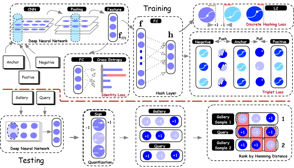
Figure 1: The framework of DVHN. It basically contains two stages. The top part illustrates the process of learning to produce effective hash codes. The bottom demonstrates the testing process. During testing, the query and gallery images are encoded into binary discrete hash codes with the trained model. Then, the gallery images are ranked by computing their Hamming distances to the query image.

II-B Vehicle ReID

A wealth of vehicle ReID methods [29][25][30] [31][6][32] have been introduced in recent years given their extensive uses in digital surveillance, intelligent transportation [33], urban computing [34]. It is challenging considering its large intra-class variation and small inter-class differences. Some works strive to boost the discriminability of the learned representations. [35] proposes a two-stream network to project vehicle images into comparable euclidean space. [3] proposes to learn feature representation by exploiting multi-grain ranking constraints. [4] further proposes to learn robust features in a coarse-to-fine fashion. In 2019, [36] adopts the vehicle part information to assist in the global feature learning. [5] introduces a novel end-to-end adversarial learning-base network to learn robust and discriminative features. [37] proposes to construct another large dataset named ”VehicleNet” and innovated a two-stage learning framework to learn robust feature representation. Another line of research focuses on learning viewpoint-invariant embedding for re-identification. Canonical examples include [30][38][39][32].[30] proposes to mine the keypoint localization information to align and extract viewpoint-invariant information. [38] further introduces a scheme which utilizes single-view input information to generate multi-view features. [39] innovates a pose-aware multi-task learning approach to learn viewpoint-invariant features. [32] introduces to disentangle the feature representation into orientation-specific and orientation-invariant features and, in the later stage, use the orientation-invariant feature to perform vehicle ReID task. [40] proposes to extract quadruple directional deep features for vehicle-re identification while [41] proposes an end-to-end distance-based deep neural network combining multi-regional features to learn to distinguish local and global differences of a vehicle image. . [42] explores vehicle parsing to learn discriminative part-level features an build a part-neighboring graph to model the correlation between every part features. To alleviate the influence of the drastic appearance variation,  [43] further introduces a novel multi-center metric learning framework which models the latent views from the vehicle visual appearance directly without the need for extra labels. Notwithstanding the successes in this literature, all the previously mentioned vehicle ReID methods are not applicable in the large-scale ReID settings where the database stores a significantly larger number of image items.

III Methodology

In this paper, we denote mapping functions with calligraphic uppercase letters, such as $\mathcal{F}$. We denote sets with bold-face uppercase letters such as $\mathbf{B}$. Images are denoted with italic uppercase letters such as $\it{I}$. Specifically, the sign activation function is represented as $\mathbf{\it{sign}}$.

III-A Problem Definition

Assume that $\mathbf{X}=\{\textit{I}_{i}\}^{N}_{i=1}$ is a training vehicle image set which contains $N$ training instances. $\mathbf{Q}=\{I_{i}^{q}\}^{N_{q}}_{i=1}$ and $\mathbf{G}=\{I^{g}_{i}\}^{N_{g}}_{i=1}$ are the query set and gallery set, respectively. $\mathbf{Y}=\{\textit{y}_{i}\}^{N}_{i=1}\in\{0,1\}^{C}$ is the corresponding label set and $C$ is the number of identities. The goal of deep hash learning for vehicle re-identification is to learn a non-linear hash function $\mathcal{H}:I\mapsto\mathbf{b}\in\{0,1\}^{K}$ which takes as input an image $\it{I}$ and map it into a K-bit binary hash code vector $\mathbf{f}$ such that the visual similarity in the raw pixel space is preserved for each vehicle image in the hamming space. The whole learning-based hash function could be formulated as:

$$\mathbf{b}=\mathcal{H}(I)=\mathbf{\it{sign}}(\mathcal{F}_{hash}(\textit{I}))$$

where $\mathcal{F}_{hash}$ stands for the non-linear deep neural network responsible for generating hash codes. I is an image. $\mathbf{\it{sign}(v)}$ returns 1 if $v\geq 0$ and returns -1 if $v<0$.

IV Proposed Model

IV-A Hashing Layer

We adopt ResNet-50 [44] as the backbone feature extraction network, which is denoted as $\mathcal{F}_{\theta}$. The feature output vector $\mathbf{f_{i}}$ for an image $I_{i}$ from $\mathcal{F}_{\theta}$ is denoted as:

$$\mathbf{f}_{i}=\mathcal{F}_{\theta}(I_{i})$$ (1)

To generate a binary hashing code of diversified lengths, we propose to devise a hashing layer on top of the backbone network. Concretely, following the global average pooling layer, we add a fully connected layer taking as input a feature vector $\mathbf{f}$ of $M$ dim and output K-dim continuous hash vector $\mathbf{h}$:

$$\mathbf{h}=\mathcal{F}_{\theta_{1}}(\mathbf{f})=\mathbf{f}W_{1}^{T}+\textbf{b}$$ (2)

where $W_{1}\in\mathbb{R}^{M\times K}$ and $\mathbf{b}\in\mathbb{R}^{K}$ denotes the weight and bias parameters while $B$ is the length of the Hamming hashing code.

IV-B Similarity-preserving Feature Learning

We organize the input vehicle into triplet samples and formulate the hash problem as a similarity preserving problem. Concretely, inspired by [14], we form input batches by first randomly sampling $P$ vehicle identities, then, we randomly sample $K_{1}$ instances for each vehicle. Thus, we get a batch of $P*K_{1}$ images in total. For every image $I_{i}$ in the batch, we will use it as an anchor image and then find an image $I_{i}^{+}$ which is the hardest positive sample for the anchor in the batch. Analogously, we can select the hardest negative sample for the anchor $I_{i}$ in the batch, which is the image belonging to another vehicle but closest to the anchor $I_{i}$ in the batch according to a predefined distance metric $D$. In doing so, a training set $\mathbf{T_{1}}=\{(I_{i},I_{i}^{+},I_{i}^{-})\}_{i=1}^{P*K_{1}}$ is derived. For each image $I$, the corresponding continuous hash vector $h$ is computed with the hash function $\mathcal{H}$:

$$h_{i}=\mathcal{H}(I_{i})=\mathcal{F}_{\theta_{1}}(\mathcal{F}_{\theta}(I_{i}))$$ (3)

where $h_{i}$ is the continuous hash vector for image $I_{i}$ and $\mathcal{F}_{\theta}$ denotes the backbone non-linear convolutional neural network structure. $\mathcal{F}_{\theta_{1}}$ denote the fully connected feed-forward neural network (hash layer) for hash code generation. Since the goal is to preserve the similarity of the images in the hamming space, it is natural to propose the following constraint:

$$\mathcal{D}_{H}(h_{i},h_{i}^{+})<\mathcal{D}_{H}(h_{i},h_{i}^{-})$$ (4)

where $\mathcal{D}_{H}$ represents the hamming distance metric. The intuition is that the hamming distance between the anchor and the hardest positive sample should be smaller than the negative counterpart. We observe a linear relation between the Hamming distance and the inner product of two vectors:

$$\mathcal{D}_{H}(h_{i},h_{j})=\frac{1}{2}(B-\langle h_{i},h_{j}\rangle)$$

Thus, in this paper, we adopt inner product as a nice surrogate for Hamming distance calculation.

In this way, we can finally formulate the triplet-based similarity preserving loss as:

$$\begin{array}[]{l}\begin{split}L_{Triplet}(h)&=\sum_{i\in\mathbf{T_{1}}}[\alpha+\mathcal{D}_{H}(h_{i},(h_{i})^{+}-\mathcal{D}_{H}(h_{i},(h_{i})^{-}]\\ &=\sum_{i=1}^{P}\sum_{a=1}^{K}[\alpha+\overbrace{\max_{p=1\ldots K}\left\|e_{i}^{a}-e_{i}^{(p)}\right\|_{2}}^{\text{hardest positive}}\\ &-\underbrace{\min_{n=1\ldots K\atop j=1\ldots P}\|e_{i}^{a}-e_{j}^{(n)}\|_{2}}_{\textrm{hardest negative}}]\end{split}\end{array}$$ (5)

where $P$ denotes the number of vehicle identities in the batch and $K$ stands for the number of instances for each identity in the batch. $e_{i}^{a}$ denotes the anchor’s vector belong to identity $i$. $\alpha$ is the margin parameter for the triplet loss.

On top of the triplet loss $L_{Triplet}$, to learn more discriminative features, we further add an Identity Loss on the feature output $\mathbf{f}$. To this end, another fully connected layer $\mathcal{F}_{\theta_{2}}$ of $N_{C}$ output logits is added after the $\mathbf{f}$ as shown in Fig. 1. $N_{C}$ is the number of vehicle identities for the training images. By regarding each vehicle identity as a class, we can formulate the identity loss $L_{Identity}$ as:

$$L_{Identity}(f)=-\sum_{i=1}^{P*K}\log\frac{e^{{W}_{y_{i}}^{T}\mathbf{f}_{i}}}{\sum_{k_{1}=1}^{N_{C}}e^{{W}_{k_{1}}^{T}\mathbf{f}_{i}}}$$ (6)

where $W_{k}$ is the weight vector for identity $k$, $P*K_{1}$ is the number of images in the batch and $N_{C}$ is the number of identities in the batch.

IV-C Discrete Hashing Learning

The core assumption is that the learned binary Hamming codes should preserve the label information. Specifically, for each image $I_{i}$, the binary Hamming code $b_{i}$ is obtained by using the sign activation function $\operatorname{sgn}(x)=\left\{\begin{array}[]{c}1,x>=0\\ -1,x\leq 0\end{array}\right.$ on the continuous hash vector $h_{i}$ as:

$$\mathbf{b}_{i}=\textit{sign}(h_{i})=\textit{sign}(\mathcal{H}(\textit{I}_{i}))$$ (7)

Similar to [45], we adopt a simple linear classifier to reconstruct the input ground-truth labels with the binary codes as:

$$y_{i}=W^{T}_{h}\mathbf{b}_{i}$$ (8)

where $y_{i}\in\{0,1\}^{C}$, $C$ is the number of identities, $W_{h}$ is the weight of the classifier for the binary codes $\mathbf{b}$. Then, we could formulate the discrete hashing loss as:

$$L_{Quant}(\mathbf{b})=\mu\sum_{i=1}^{N}\left\|y_{i}-W^{T}_{h}\mathbf{b}_{i}\right\|_{2}^{2}+\nu\|W_{h}\|_{F}^{2}$$ (9)

where $\|\cdot\|_{2}$ is the $l2$ norm of a vector while $\|\cdot\|_{F}$ is the Frobenius norm of a specific matrix.

IV-D Alternative Optimization

We formulate the final total loss function as:

$$L_{Total}=\lambda L_{Triplet}(\mathbf{h})+\sigma L_{Identity}(\mathbf{f})+L_{Quant}(\mathbf{b})$$ (10)

where $\lambda$, $\beta$ and $\sigma$ are three predefined coefficients for controlling the influence of each individual loss. One might ponder the possibility of optimizing the Eq. 10 with standardized stochastic gradient descent. Nonetheless, the sign function is non-differentiable which can not be directly optimized by back-propagating the gradients. Thus, the third term $L_{Quant}(\mathbf{b})$ could not be optimized in a same way as the first two terms. We, thus, unfold the last term in the Eq. 10:

$$L_{Total} =\lambda L_{Triplet}(\mathbf{h})+\sigma L_{Identity}(\mathbf{f}))$$ (11)

$$+\mu\sum_{i=1}^{N}\left\|y_{i}-W_{h}^{T}b_{i}\right\|_{2}^{2}+\nu\|W_{h}\|_{F}^{2}$$

To circumvent the vanishing gradient problem introduced by sign, some previous works adopts tanh or sigmoid activation function to generate continuous outputs which are the relaxation of the binary Hamming codes in the training stage. In the testing stage, sign activation function is adopted to obtain the corresponding binary Hamming hashing codes. However, such an optimization scheme is optimizing a relaxed surrogate of the original target and will result in learning sub-optimal Hamming hashing codes owing to the sizable Quantization Error [25].

In this regard, we propose to adopt a novel Alternative Optimization scheme which considers the discrete nature of binary codes by constraining the outputs from the deep neural network to be binary codes directly. Similar to [46, 45], we introduce an auxiliary variable and derive an approximation of Eq. 11 as:

$$L_{Total} =L_{Triplet}(h)+L_{Identity}(f)$$ (12)

$$+\mu\sum_{i=1}^{N}\left\|y_{i}-W_{h}^{T}b_{i}\right\|_{2}^{2}+\nu\|W_{h}\|_{F}^{2}$$

$$\text{ s.t. }\quad\mathbf{b}_{i}=\operatorname{sgn}\left(h_{i}\right),\quad\mathbf{h}_{i}\in\mathbb{R}^{K\times 1},\quad(i=1,\ldots,N)$$

where $\mathbf{h}=\mathcal{F}_{hash}(f)$ is the continuous hashing vector, $\mathbf{f}$ is the feature output from the deep convolutional neural network and $\mathbf{b}$ is the binarized Hamming hashing code. The above equation is a constrained optimization problem, which could be solved with the Lagrange Multiplier Method as:

$$L_{Total} =L_{Triplet}(h)+L_{Identity}(f)$$ (13)

$$+\mu\sum_{i=1}^{N}\left\|y_{i}-W^{T}_{h}b_{i}\right\|_{2}^{2}+\nu\|W_{h}\|_{F}^{2}$$

$$+\eta\sum_{i=1}^{N}\left\|\mathbf{b}_{i}-\operatorname{sgn}\left(\mathbf{h}_{i}\right)\right\|_{2}^{2}$$

$$\text{ s.t. }\quad\mathbf{b}_{i}\in\{-1,1\}^{K},\quad\mathbf{h}_{i}\in\mathbb{R}^{K\times 1},\quad(i=1,\ldots,N)$$

The last term can also be viewed as a constraint which measures the quantization error between the continuous hashing feature vector and its binarized Hamming code. Inspired by [45], we decouple the above optimization target Eq. 13 into two sub optimization problem, and solve them in an alternative fashion.

First, we fix $b$ and $W$, the optimization target is converted to

$$L =\lambda L_{Triplet}(\mathbf{h})+\sigma L_{Identity}(\mathbf{f})$$ (14)

$$+\eta\sum_{i=1}^{N}\left\|\mathbf{b}_{i}-\mathbf{h}_{i}\right\|_{2}^{2}$$

Then, the parameters of the backbone $\theta$, hash layer $\theta_{1}$, and the identity loss $\theta_{2}$ could be updated with standard Stochastic Gradient Descent and Back Propagation algorithm.

Secondly, we fix the parameters $\theta$, $\theta_{1}$, $\theta_{2}$ and $\mathbf{b}_{i}$ and the problem is converted into:

$$L=\mu\sum_{i=1}^{N}\left\|y_{i}-W_{h}^{T}b_{i}\right\|_{2}^{2}+\nu\|W_{h}\|_{F}^{2}\\$$ (15)

It is obvious to note that this is a Least Squares problem and has a closed-form solution as:

$$W_{h}=\left(BB^{T}+\frac{\nu}{\mu}I\right)^{-1}B^{T}Y$$ (16)

where $B=\{\mathbf{b}_{i}\}_{i=1}^{N}\in\{-1,1\}^{K\times N}$ and $Y=\{y_{i}\}^{N}_{i=1}\in\mathbb{R}^{C\times N}$.

Finally, after solving $W_{h}$, when we fix the parameters $\theta$, $\theta_{1}$, $\theta_{2}$ and $W_{h}$, we obtain the final objective as:

$$L=\mu\sum_{i=1}^{N}\left\|y_{i}-W_{h}^{T}\mathbf{b}_{i}\right\|_{2}^{2}+\eta\sum_{i=1}^{N}\left\|\mathbf{b}_{i}-\mathbf{h}_{i}\right\|_{2}^{2}$$ (17)

$$\text{ s.t. }\quad\mathbf{b}_{i}\in\{-1,1\}^{K},(i=1,\ldots,N)$$

Inspired by [45], we adopt the discrete cyclic coordinate descent method to solve $B$ row by row in an iterative fashion as:

$$\min_{B}\left\|W_{h}^{T}B\right\|^{2}-2\operatorname{Tr}(P),\quad\text{ s.t. }B\in\{-1,1\}^{K\times N}$$ (18)

where $P=W_{h}Y+\frac{\eta}{\mu}H$. The overall training algorithm for DVHN is illustrated in Algo. 1.

Input: Training vehicle image set $\mathbf{T}$, labels $\mathbf{Y}$,  learning rate $\epsilon$ and parameters $\lambda$, $\beta$, $\sigma$,  the margin parameter $\alpha$,  maximum training iteration $T$

Output: network parameters $\theta$, $\theta_{1}$, $\theta_{2}$, $W_{h}$, $\mathbf{B}$;

1 Initialize: the resnet-50 network parameters $\theta$ with pretrained weights on ImageNet, $\theta_{1},\theta_{2},W_{h},B$ with random values, and t = 0

2 while not converged and $t<T$  do

3       $t=t+1$;

4       for $i\leftarrow 0$ to $100$  do

5             Freeze $W,b$ ;

6             Sample $P$ vehicle identities. Then sample $K$ instances for each $p\in P$, resulting in a batch image set $\mathbf{B}=\{I_{i}\}_{i=1}^{P*K}$ and the corresponding label set $\mathbf{Y}=\{y_{i}\}_{i=1}^{p*K}$;

7             For each image $I_{i}$, calculate $f_{i}=\mathcal{F}_{\theta}(I_{i})$ ;

8             Calculate continuous hash vector $h_{i}=\mathcal{F}_{\theta_{1}}(f_{i})$ ;

9             Obtain loss $L_{Identity}$ by Eq. 6 ;

10             Construct triplet set $\{h_{i},h_{i}^{+},h_{i}^{-}\}$ ;

11             Obtain loss $L_{Triplet}$ by Eq. 5 ;

12            

13            Use SGD to get gradients $\nabla_{\theta_{*}}$ $*\in\{\theta,\theta_{1},\theta_{2}\}$ for Eq. 14;

14             Update $\theta_{*}=\alpha(\theta_{*}-\nabla_{\theta_{*}})$ ;

15            

16       end for

17      Freeze $\theta,~{}\theta_{1},~{}\theta_{2}$, update $W_{h}$ with Eq. 16 ;

18       Freeze $\theta,~{}\theta_{1},~{}\theta_{2},W_{h}$, update $\mathbf{B}$ through Eq.18

19 end while

Algorithm 1 Optimization Algorithm for DVHN

IV-E Retrieval Process

In this section, we elaborate on how to perform efficient vehicle re-identification given the trained model. Generally, we are given a query image set $\mathbf{Q}$ and a gallery image set $\mathbf{G}$. For each query image $q_{k}$, the task is to identify the images in $\mathbf{G}$ belonging to the same vehicle. In the testing phase, for each query image $q_{k}$, we obtain the discrete binary code vector $\mathbf{b}_{k}^{q}$ through:

$$\mathbf{b}_{k}^{q}=\mathbf{\it{sign}(\mathcal{F}_{\theta_{1}}(\mathcal{F}_{\theta}(\it{I}^{q}_{k})))}$$ (19)

Subsequently, in a same fashion, for all the images in $\mathbf{G}=\{\it{I}^{g}_{k}\}_{k=1}^{N_{g}}$, we obtain a set of binary code vectors $\mathbf{H^{g}}=\{\mathbf{b}_{k}^{g}\}_{k=1}^{N_{g}}$. Then, we can rank the gallery code vectors through their hamming distance with respect to the query image code vector. We note that there is a linear relationship between inner product $\langle\cdot,\cdot\rangle$ and hamming distance $\mathcal{D}_{H}$, which is stated as:

$$\mathcal{D}_{H}(\mathbf{b}_{i},\mathbf{b}_{j})=\frac{1}{2}(B-\langle\mathbf{b}_{i},\mathbf{b}_{j}\rangle)$$

where $K$ is the bit length of the binary hashing code $\mathbf{b}$. The above equation makes the inner product a nice surrogate for hamming distance computing. In the later stage, we compute the hamming distance between $\mathbf{b}_{k}^{q}$ and all the gallery hash codes in $G$. Then, we sort the distances in an increasing order. Finally, we rank the images in $\mathbf{G}$ according to the sorted hamming distances.

V Experiments

V-A Implementation Details

We implement our model with pytorch [47]. The detailed framework is illustrated in Fig. 1. Specifically, after the final $f_{avg}$ layer of resnet50, we add a fully connected layer of $K$ output logits where $K$ denotes the hash code length. For the classification stream, we added another fully connected layer of $N_{C}$ output logits, $N_{C}$ denoting the number of classes. These two additional layers are initialized with ”normal” initialization, the mean being $0$ and standard deviation being $0.01$. In the training process, the number of identities $P$ is set to 16, and the number of instances is $6$, resulting in a batch of 96 images. During training, the parameters are optimized with ”amsgrad” optimizer. The initial learning rate $\epsilon$ is set to $3e-4$, the weight decay to $\it{5e-4}$, the beta1 to 0.9, and the beta2 to 0.99. The margin parameter $\alpha$ in Eq. 5 is set to $0.3$. For the coefficients controlling the influence of each loss $(\lambda,\beta,\sigma)$, we empirically set all of them to $1$

V-B Datasets and Evaluation Protocols

Datasets. We conduct experiments on two widely-studied public datasets: VehicleID [1] and VeRi [25]. VehicleID is a large-scale vehicle re-identification dataset containing 221763 images of 26267 vehicle identities in total. Among all the images, 110,178 images of 13,134 vehicles are selected for training. For testing, three subsets which contain 800, 1600, 2400 vehicles are extracted from the testing dataset and are denoted as 800, 1600, 2400, respectively. We empirically evaluated the performances of our model on 800 and 1600 scenario. Specifically, for 800, the query set contains 5693 images of 800 vehicle identities, and the gallery dataset contains 800 images in total, one for each vehicle identity. In a similar fashion, for the 1600 scenario, the query set comprises 11777 images of 1600 cars, while the gallery set contains 1600 images of 1600 identities. VeRi is a real-world urban surveillance vehicle dataset containing over 50000 images of 776 vehicle identities, among which 37781 images of 576 vehicles are designated as the training set. For testing, 1678 images of 200 vehicles are designated as the query set, while the gallery contains 11579 for the same 200 vehicles.
Evaluation Protocols. We evaluate our model on two widely-adopted metrics: cumulative matching characteristics (CMC) and mean average precision (mAP). The CMC score computes the probability that a query image appears in a different-sized retrieval list. However, it only counts the first match, making it unsuitable in a scenario where the gallery contains more than one image for each query. Thus, we also employ mAP, which, essentially, takes into consideration both the precision and recall of the retrieved results.

TABLE I: Vehicle Re-identification Results of State-of-The-Art Deep Hash Methods on Vehicle (800 and VeRi

Datasets	VehicleID (800)				VeRi
Methods	256	512	1024	2048	256	512	1024	2048
SH[16] (NeurIPS)	23.98	23.64	21.09	17.71	3.33	2.75	2.08	1.57
ITQ[17] (TPAMI)	23.84	25.39	25.93	26.26	4.80	4.95	5.04	5.14
DSH[48] (CVPR)	30.56	32.53	34.22	33.62	8.93	9.77	10.24	10.47
DHN[24] (AAAI)	43.57	45.42	46.70	46.39	13.85	13.93	14.31	13.71
HashNet[11] (ICCV)	62.95	64.52	65.96	66.61	27.13	28.40	29.94	29.30
DCH[13] (CVPR)	37.08	34.55	26.04	24.13	19.75	19.23	12.15	14.96
DPN[22] (IJCAI)	57.16	61.92	63.55	64.65	10.03	11.26	13.52	13.58
DVHN	71.61	73.69	75.86	76.82	54.61	58.38	59.27	62.02

TABLE II: Vehicle Re-identification Results of State-of-The-Art Deep Hash Methods (VehicleID (1600))

Datasets	VehicleID (800)
Methods	256	512	1024	2048
SH[16] (NeurIPS)	19.96	20.06	16.32	13.83
ITQ[17] (TPAMI)	20.23	21.45	21.27	22.23
DSH[48] (CVPR)	26.25	29.39	30.36	30.97
DHN[24] (AAAI)	39.97	41.77	43.34	43.72
HashNet[11] (ICCV)	56.89	69.99	60.05	60.88
DCH[13] (CVPR)	27.23	25.33	19.67	18.45
DPN[22] (IJCAI)	53.68	58.03	60.23	61.42
DVHN	66.67	69.12	71.83	72.72

V-C Comparisons with State-of-the-arts

In this section, we compare the results of our proposed DVHN and the state-of-the-art deep hash methods. Specifically, the competing methods could be divided into two categories: unsupervised hash methods and supervised hash methods. For the unsupervised methods, we include SH [16] and ITQ [17]. Note that these two methods are reliant upon extra feature extractors to get feature representations for the dataset. To this end, we adopt AlexNet which is pretrained on ImageNet to extract features. For the supervised setting, we further incorporate DSH [48] which was among the first works attempting to learn discrete hamming hash codes with deep convolutional neural networks. In addition, we incorporate other recent methods for detailed comparisons and analyses including  DHN [24], HashNet [11], DCH, [13] DPN [22]. Note that we adopt original source codes for SH, ITQ,  DCH and DHN. For other methods, we implement them with pytorch. We first provide analysis for the results of all the models with 2048 hash bits. It is rather evident from Tab. I and Tab. II that traditional unsupervised methods like SH and ITQ exhibit significant poorer performance across two datasets. Their mAP scores on VeRi are 1.57% and 5.14% when the hashing bit length equals $2048$, respectively. On VehicleID (800) and VehicleID (1600), the performance are slightly better. Specifically, Sh achieves mAPs of 17.71% and 13.83% while ITQ reaches 26.26% and 22.23% for 2048 bits on these two datasets. The unsatisfactory results could in large part be attributed to the fact that unsupervised methods could not learn the discriminative features, leading to sub-optimal hash codes. Clearly, supervised methods achieve better results across two datasets for all the hashing bit lengths. Especially, HashNet and DPN achieve pronounced results on VehicleID (800), 66.61% and 64.65% for $2048$ bits, respectively. Across other hashing bit lengths, they are also clear winners regarding mAP. In terms of VeRi, poorer performance could be spotted, 29.30% mAP for HashNet and 13.58% for DPN on 2048 bits. The degraded performance could result from the small discrepancy of images from the same vehicle. Unsurprisingly, our proposed DVHN is a clear winner against all the competing methods across all the compared bit lengths. Concretely, we achieve the state-of-the-art results with pronounced margins of 11.05% and 35.46% in terms of Rank@1 on VehicleID and VeRi on 2048 bits, respectively. For 256 bits, we obtain 11.54% and 30.93% performance improvements of Rank@1. In terms of mAP, for 2048 bits, we achieve 76.82%, 72.72% and 56.57% on VehicleID (800), VehicleID (1600) and VeRi, outperforming the second-best results by 10.21%, 11.30% and 32.72%. The superior performances collectively and evidently demonstrated the advantages of the joint hash and classification stream design, which enables the model to learn more discriminative features.

We further provide the top-K accuracy results (CMC curves) of different hash bit lengths on VehicleID (800), VehicleID (1600) and VeRi in Fig. 2 .

VehicleID (800). As depicted in Fig. 2, we compare the CMC results of our model DVHN with other state-of-the-art deep supervised hash methods across four different hashing bit lengths. Note that we do not include two unsupervised counterparts into comparisons considering their unsatisfactory performance in this domain. Evidently, DVHN achieves notable results especially from Rank@1 to Rank@5. Specifically, we achieve 11.52%, 9.61%, 10.75% and 11.05% performance gains against DPN in 256, 512, 1024 and 2048 hash bits. It is also easy to note that HashNet can achieve comparable performance from Rank@6 to Rank@20 when hash bit length equals 256 and 512. However, in terms of vehicle re-identification task, it is of crucial importance that the relative matching images appear in the front of the retrieval list. In terms of mAP, as depicted in the above part of Fig. 2, DVHN beats all the other competing methods with notable margins. It is also easy to spot that with the number of bits increasing, our proposed model achieves growing mAP scores from 71.61% to 76.81%. The performance gain could be attributed to the fact that the model capture more information with a comparatively larger hash bit length.

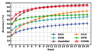
(a) CMC Results of VehicleID (800) of 256 bits

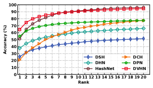
(b) CMC Results of VehicleID (800) of 512 bits

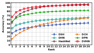
(c) CMC Results of VehicleID (800) of 1024 bits

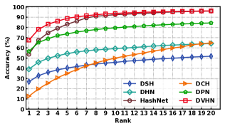
(d) CMC Results of VehicleID (800) of 2048 bits

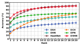
(e) CMC Results of VehicleID (1600) of 256 bits

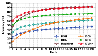
(f) CMC Results of VehicleID (1600) of 512 bits

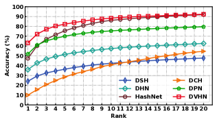
(g) CMC Results of VehicleID (1600) of 1024 bits

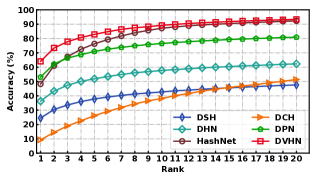
(h) CMC Results of VehicleID (1600) of 2048 bits

(i) CMC Results of VeRi of 256 bits

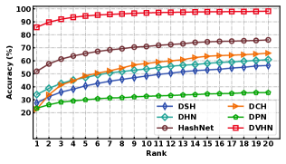
(j) CMC Results of VeRi of 512 bits

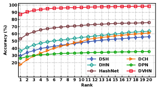
(k) CMC Results of VeRi of 1024 bits

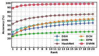
(l) CMC Results of VeRi of 2048 bits

Figure 2: The Cumulative Matching Characteristics (CMC) results against the State-of-the-art methods on three datasets across 256, 512, 1024, 2048 hashing bits

VehicleID (1600). For test performance on this scenario, as demonstrated in Fig. 2, a similar trend is spotted for both CMC and mAP. We achieve 57.06%, 60.41%, 63.26% and 64.11% of Rank@1 for 256, 512, 1024 and 2048 hash bits respectively. In regard to mAP, we outperform all the candidate methods by large margins in all testing scenarios. Note that, when compared with performance on VehicleID(800), the model experiences moderate performance declines for all hash bits. For instance, the Rank@1 accuracy drops by over 4% for hash bit 256 while the mAP drops by near 5%. The degraded performance is mainly due to the introduced difficulty of larger gallery set.

VeRi. As is manifested in Fig. 2, DVHN exhibits consistent advantages against all the competing method across all the evaluation metrics. Specifically, as shown in Fig. 2, DVHN outperforms HashNet by large margins, consistently. We achieve 80.10%, 85.81%, 87.01% and 88.62% of Rank@1 for 256, 512, 1024 and 2048 bits, beating HashNet by 30.93%, 33.85%, 33.73% and 35.46%. Similar performance gains could be spotted for other hash bit lengths. As for mAP, the performance gap between our model and other methods is even more pronounced. We outperform the second best model by 32.77% when hash bit length equals 2048. It is obvious to note that in Fig. 2, the curve of DVHN which is colored red consistently levitates above other competing methods with notable margins. The superiority of our method could mainly be attributed to the joint design of the similarity-preserving learning and the discrete hashing learning.

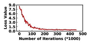
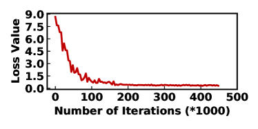
(a) The convergence curve of DVHN on 256 (left) and 512 (right) bits.

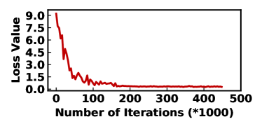
(b) The convergence curve of DVHN on 1024 (left) and 2048 (right) bits.

Figure 3: The Convergence Analysis of DVHN of 256, 512, 1024 and 2048 bits.

(a) Query Time on VehicleID (1600)

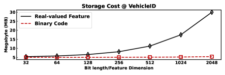
(b) Storage Cost on VehicleID (1600)

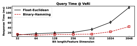
(c) Query Time on VeRi

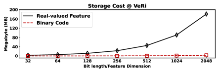
(d) Storage Cost on VeRi

Figure 4: Comparison of the total query response time and storage cost of

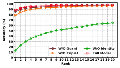
(a) The CMC results of different variants on VeRi dataset

(b) The CMC results of different variants on VehicleID (800)) dataset

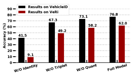
(c) The mAP results of different variants on both VeRi and VehicleID(800) datasets

Figure 5: The CMC and mAP Results of DVHN and Its Three Variants

V-D Empirical Analysis

First, we plot the convergence curves for our model across four hashing bits in Fig. 3.

Second, we conduct a detailed ablation study to demonstrate the effectiveness of each component of our proposed DVHN. To effectively evaluate the importance of Identity Loss ($L_{Identity}$), triplet-based hash loss ($L_{Triplet}$), and the proposed discrete learning loss ($L_{Quant}$), we empirically test the performance of our model on VehicleID (800) and VeRi when stripped of each component. We denote the model of all the component as Full Model, the model without triplet loss as W/O Triplet, the model without Identity Loss as W/O Identity and, finally, the model without the discrete hashing learning as W/O Quant. Note that all the experiments were conducted on 2048 hash bits. As demonstrated in Fig. 5(a) and Fig. 5(b), when the discrete learning loss is moved from the model, we experience slight performance declines, 3.46% and 3.5% for Rank@1 and mAP on VehicleID (800), and 2.80% and 3.77% for Rank@1 and mAP on VeRi. This evidences the validity of the discrete hashing learning module for the binary Hamming hashing codes to preserve the class information. When deprived of the identity loss, the model experience conspicuous performance decreases. On VehicleID (800), the Rank@1 accuracy drops by 40.84% while the mAP score drops by 35.31%. On VeRi, the performance deterioration is even more severe, 75.11% for Rank@1 and 52.84% for mAP. The declines have demonstrated the importance of the identity loss on learning more robust and discriminative features. Finally, when looking at the performance of W/O Triplet, we could also spot notable performance declines against the Full Model. W/O Triplet achieves 57.47% of Rank@1 accuracy and 67.32% mAP, 10.19% and 9.45% smaller than its full model counterpart on VehicleID (800). On VeRi, a similar trend can also be spotted when the model is depried of $L_{Triplet}$. W/O Triplet achieves 78.84% of Rank@1 and 49.23% of mAP, 9.78% and 12.79% lower than the Full Model counterpart.The deterioration is largely due to the effectiveness of batch-hard triplet loss in tackling the vehicle re-identification problem, where the intra-class variation is sometimes even larger than the inter-class variation. Finally, as elaborated above, all the proposed components are essential to the final performance of the proposed final model.

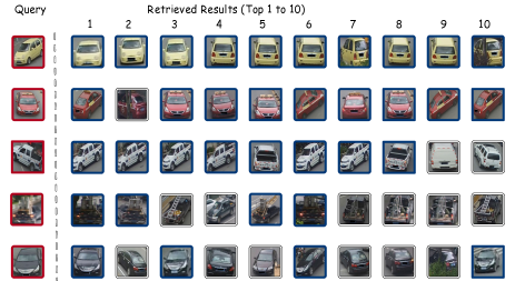
(a) Retrieved Results

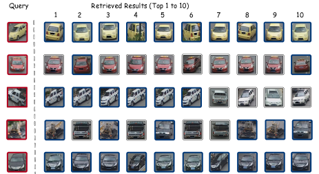
(b) CMC Results of on VehicleID (800) of 512 bits

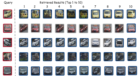
(c) Retrieved Results

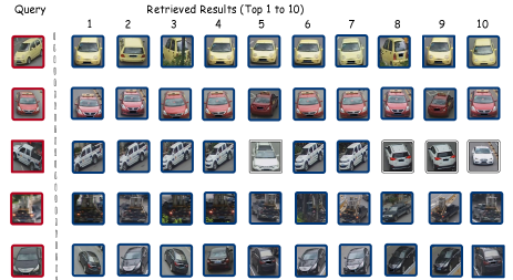
(d) CMC Results of on VehicleID (1600) of 256 bits

Figure 6: The Visualization of the Top 10 Retrieved Results of Our Framework on 256, 512, 1024, 2048 Hashing Bits.

V-E Retrieval Efficiency Comparison

The time cost of a Vehicle ReID system generally is comprised of two separate parts: feature extraction cost and similarity calculation cost. As is pointed out by [49], the cost of the feature extraction actually heavily depends on the backbone network used. Thus, we focus on comparing the large-scale similarity calculation time costs of our method and the real-valued vehicle re-identification counterparts. Meanwhile, we also compare the storage costs of our Hamming hashing re-identification framework with the real-valued ones.

Specifically, we illustrate the results on VehicleID (1600) and VeRi in Fig. 4, which have (11777, 1600), (1678, 11579) (query, gallery) images, respectively. In Fig. 4(a) and Fig. 4(c), the ’Float-Euclidean’ denotes the query time for Euclidean distance based real-valued vehicle re-identification methods while ’Binary-Hamming’ denotes the query time for our binary hashing method with Hamming distance calculation. For Fig. 4(b) and Fig. 4(d), it demonstrates the comparison of storage cost on VehicleID (1600) and VeRi for real-valued methods and our binary Hamming codes based method. It is obvious that binary codes could save tremendous memory compared with its real-valued counterparts.

V-F Qualitative Analysis of the Retrieved Results

In Fig. 6, we visualize the retrieval results for different hash bit length of our model in VeRi. Note that, to demonstrate the retrieval efficiency, we take the original gallery set as a query set so that for each query image, there exist several images in the gallery set. In the picture above, we adopt the same query images for four testing scenarios where the hash bit length equals 256, 512, 1024 and 2048, respectively. The right part visualizes the retrieval list for the query image. The image enclosed by a red box means it is from the same vehicle as the query image. Generally, for a re-identification model, it would be desirable for the matching images to appear in the front of the retrieval list.

VI Conclusion

In this paper, we propose DVHN, a deep hashing based framework for efficient large-scale vehicle re-identification. Contrary to conventional method which adopt real-valued feature vectors to perform re-identification task, we adopt a Hamming hashing-based scheme which saves tremendous memory and is much faster in terms of retrieval speed and thus, could be applied in a large-scale re-identification scenario. Specifically, for similarity-preserving learning, we adopt a triplet loss and an on-the-fly hard triplet generation module. Meanwhile, we further add an identity loss to learn more robust and discriminative features. For binary code learning, we propose a discrete hashing learning scheme which is based on the assumption that the binary codes should be ideal for classification. To overcome the vanishing gradient problem (the sign function for generating binary codes is not differentiable), we adopt an alternative optimization method for optimizing the overall framework. We conduct extensive experiments and the results have demonstrated that our framework could generate discriminative binary codes for efficient vehicle re-identification, surpassing the stet-of-the-art hashing methods with large margins.

References

- [1] H. Liu, Y. Tian, Y. Yang, L. Pang, and T. Huang, “Deep relative distance learning: Tell the difference between similar vehicles,” in Proceedings of the IEEE conference on computer vision and pattern recognition, 2016, pp. 2167–2175.
- [2] W. Liu, X. Liu, H. Ma, and P. Cheng, “Beyond human-level license plate super-resolution with progressive vehicle search and domain priori gan,” in Proceedings of the 25th ACM international conference on Multimedia, 2017, pp. 1618–1626.
- [3] K. Yan, Y. Tian, Y. Wang, W. Zeng, and T. Huang, “Exploiting multi-grain ranking constraints for precisely searching visually-similar vehicles,” in Proceedings of the IEEE international conference on computer vision, 2017, pp. 562–570.
- [4] H. Guo, C. Zhao, Z. Liu, J. Wang, and H. Lu, “Learning coarse-to-fine structured feature embedding for vehicle re-identification,” in Proceedings of the AAAI Conference on Artificial Intelligence, vol. 32, no. 1, 2018.
- [5] Y. Lou, Y. Bai, J. Liu, S. Wang, and L.-Y. Duan, “Embedding adversarial learning for vehicle re-identification,” IEEE Transactions on Image Processing, vol. 28, no. 8, pp. 3794–3807, 2019.
- [6] D. Meng, L. Li, X. Liu, Y. Li, S. Yang, Z.-J. Zha, X. Gao, S. Wang, and Q. Huang, “Parsing-based view-aware embedding network for vehicle re-identification,” in Proceedings of the IEEE/CVF Conference on Computer Vision and Pattern Recognition, 2020, pp. 7103–7112.
- [7] R. Chu, Y. Sun, Y. Li, Z. Liu, C. Zhang, and Y. Wei, “Vehicle re-identification with viewpoint-aware metric learning,” in Proceedings of the IEEE/CVF International Conference on Computer Vision, 2019, pp. 8282–8291.
- [8] K. Lin, H.-F. Yang, J.-H. Hsiao, and C.-S. Chen, “Deep learning of binary hash codes for fast image retrieval,” in Proceedings of the IEEE conference on computer vision and pattern recognition workshops, 2015, pp. 27–35.
- [9] F. Cakir, K. He, S. A. Bargal, and S. Sclaroff, “Hashing with mutual information,” IEEE transactions on pattern analysis and machine intelligence, vol. 41, no. 10, pp. 2424–2437, 2019.
- [10] Y. Cao, M. Long, J. Wang, and H. Zhu, “Correlation autoencoder hashing for supervised cross-modal search,” in Proceedings of the 2016 ACM on International Conference on Multimedia Retrieval, 2016, pp. 197–204.
- [11] Z. Cao, M. Long, J. Wang, and P. S. Yu, “Hashnet: Deep learning to hash by continuation,” in Proceedings of the IEEE international conference on computer vision, 2017, pp. 5608–5617.
- [12] E.-J. Ong and M. Bober, “Improved hamming distance search using variable length substrings,” in Proceedings of the IEEE Conference on Computer Vision and Pattern Recognition, 2016, pp. 2000–2008.
- [13] Y. Cao, M. Long, B. Liu, and J. Wang, “Deep cauchy hashing for hamming space retrieval,” in Proceedings of the IEEE Conference on Computer Vision and Pattern Recognition, 2018, pp. 1229–1237.
- [14] A. Hermans, L. Beyer, and B. Leibe, “In defense of the triplet loss for person re-identification,” arXiv preprint arXiv:1703.07737, 2017.
- [15] P. Indyk, R. Motwani, P. Raghavan, and S. Vempala, “Locality-preserving hashing in multidimensional spaces,” in Proceedings of the twenty-ninth annual ACM symposium on Theory of computing, 1997, pp. 618–625.
- [16] Y. Weiss, A. Torralba, R. Fergus, et al., “Spectral hashing.” in Nips, vol. 1, no. 2. Citeseer, 2008, p. 4.
- [17] Y. Gong, S. Lazebnik, A. Gordo, and F. Perronnin, “Iterative quantization: A procrustean approach to learning binary codes for large-scale image retrieval,” IEEE transactions on pattern analysis and machine intelligence, vol. 35, no. 12, pp. 2916–2929, 2012.
- [18] J.-P. Heo, Y. Lee, J. He, S.-F. Chang, and S.-E. Yoon, “Spherical hashing,” in 2012 IEEE Conference on Computer Vision and Pattern Recognition. IEEE, 2012, pp. 2957–2964.
- [19] H. Jegou, M. Douze, and C. Schmid, “Product quantization for nearest neighbor search,” IEEE transactions on pattern analysis and machine intelligence, vol. 33, no. 1, pp. 117–128, 2010.
- [20] T. Ge, K. He, Q. Ke, and J. Sun, “Optimized product quantization,” IEEE transactions on pattern analysis and machine intelligence, vol. 36, no. 4, pp. 744–755, 2013.
- [21] M. S. Charikar, “Similarity estimation techniques from rounding algorithms,” in Proceedings of the thiry-fourth annual ACM symposium on Theory of computing, 2002, pp. 380–388.
- [22] L. Fan, K. W. Ng, C. Ju, T. Zhang, and C. S. Chan, “Deep polarized network for supervised learning of accurate binary hashing codes,” in Proceedings of the Twenty-Ninth International Joint Conference on Artificial Intelligence, IJCAI-20, pp. 825–831.
- [23] W.-J. Li, S. Wang, and W.-C. Kang, “Feature learning based deep supervised hashing with pairwise labels,” arXiv preprint arXiv:1511.03855, 2015.
- [24] H. Zhu, M. Long, J. Wang, and Y. Cao, “Deep hashing network for efficient similarity retrieval,” in Proceedings of the AAAI Conference on Artificial Intelligence, vol. 30, no. 1, 2016.
- [25] X. Liu, W. Liu, T. Mei, and H. Ma, “A deep learning-based approach to progressive vehicle re-identification for urban surveillance,” in European conference on computer vision. Springer, 2016, pp. 869–884.
- [26] R. Xia, Y. Pan, H. Lai, C. Liu, and S. Yan, “Supervised hashing for image retrieval via image representation learning,” in Proceedings of the AAAI conference on artificial intelligence, vol. 28, no. 1, 2014.
- [27] H. Lai, Y. Pan, Y. Liu, and S. Yan, “Simultaneous feature learning and hash coding with deep neural networks,” in Proceedings of the IEEE conference on computer vision and pattern recognition, 2015, pp. 3270–3278.
- [28] D. Wu, Q. Dai, J. Liu, B. Li, and W. Wang, “Deep incremental hashing network for efficient image retrieval,” in Proceedings of the IEEE/CVF Conference on Computer Vision and Pattern Recognition, 2019, pp. 9069–9077.
- [29] X. Liu, W. Liu, H. Ma, and H. Fu, “Large-scale vehicle re-identification in urban surveillance videos,” in 2016 IEEE International Conference on Multimedia and Expo (ICME). IEEE, 2016, pp. 1–6.
- [30] Z. Wang, L. Tang, X. Liu, Z. Yao, S. Yi, J. Shao, J. Yan, S. Wang, H. Li, and X. Wang, “Orientation invariant feature embedding and spatial temporal regularization for vehicle re-identification,” in Proceedings of the IEEE International Conference on Computer Vision, 2017, pp. 379–387.
- [31] X. Liu, W. Liu, T. Mei, and H. Ma, “Provid: Progressive and multimodal vehicle reidentification for large-scale urban surveillance,” IEEE Transactions on Multimedia, vol. 20, no. 3, pp. 645–658, 2017.
- [32] Y. Bai, Y. Lou, Y. Dai, J. Liu, Z. Chen, L.-Y. Duan, and I. Pillar, “Disentangled feature learning network for vehicle re-identification.”
- [33] J. Zhang, F.-Y. Wang, K. Wang, W.-H. Lin, X. Xu, and C. Chen, “Data-driven intelligent transportation systems: A survey,” IEEE Transactions on Intelligent Transportation Systems, vol. 12, no. 4, pp. 1624–1639, 2011.
- [34] Y. Zheng, L. Capra, O. Wolfson, and H. Yang, “Urban computing: concepts, methodologies, and applications,” ACM Transactions on Intelligent Systems and Technology (TIST), vol. 5, no. 3, pp. 1–55, 2014.
- [35] H. Liu, Y. Tian, Y. Yang, L. Pang, and T. Huang, “Deep relative distance learning: Tell the difference between similar vehicles,” in Proceedings of the IEEE conference on computer vision and pattern recognition, 2016, pp. 2167–2175.
- [36] B. He, J. Li, Y. Zhao, and Y. Tian, “Part-regularized near-duplicate vehicle re-identification,” in Proceedings of the IEEE/CVF Conference on Computer Vision and Pattern Recognition, 2019, pp. 3997–4005.
- [37] Z. Zheng, T. Ruan, Y. Wei, Y. Yang, and T. Mei, “Vehiclenet: learning robust visual representation for vehicle re-identification,” IEEE Transactions on Multimedia, 2020.
- [38] Y. Zhou and L. Shao, “Aware attentive multi-view inference for vehicle re-identification,” in Proceedings of the IEEE conference on computer vision and pattern recognition, 2018, pp. 6489–6498.
- [39] Z. Tang, M. Naphade, S. Birchfield, J. Tremblay, W. Hodge, R. Kumar, S. Wang, and X. Yang, “Pamtri: Pose-aware multi-task learning for vehicle re-identification using highly randomized synthetic data,” in Proceedings of the IEEE/CVF International Conference on Computer Vision, 2019, pp. 211–220.
- [40] J. Zhu, H. Zeng, J. Huang, S. Liao, Z. Lei, C. Cai, and L. Zheng, “Vehicle re-identification using quadruple directional deep learning features,” IEEE Transactions on Intelligent Transportation Systems, vol. 21, no. 1, pp. 410–420, 2019.
- [41] X. Chen, H. Sui, J. Fang, W. Feng, and M. Zhou, “Vehicle re-identification using distance-based global and partial multi-regional feature learning,” IEEE Transactions on Intelligent Transportation Systems, vol. 22, no. 2, pp. 1276–1286, 2020.
- [42] X. Liu, W. Liu, J. Zheng, C. Yan, and T. Mei, “Beyond the parts: Learning multi-view cross-part correlation for vehicle re-identification,” in Proceedings of the 28th ACM International Conference on Multimedia, 2020, pp. 907–915.
- [43] Y. Jin, C. Li, Y. Li, P. Peng, and G. A. Giannopoulos, “Model latent views with multi-center metric learning for vehicle re-identification,” IEEE Transactions on Intelligent Transportation Systems, vol. 22, no. 3, pp. 1919–1931, 2021.
- [44] K. He, X. Zhang, S. Ren, and J. Sun, “Deep residual learning for image recognition,” in Proceedings of the IEEE conference on computer vision and pattern recognition, 2016, pp. 770–778.
- [45] Q. Li, Z. Sun, R. He, and T. Tan, “Deep supervised discrete hashing,” arXiv preprint arXiv:1705.10999, 2017.
- [46] X. Wang, Y. Shi, and K. M. Kitani, “Deep supervised hashing with triplet labels,” in Asian conference on computer vision. Springer, 2016, pp. 70–84.
- [47] A. Paszke, S. Gross, F. Massa, A. Lerer, J. Bradbury, G. Chanan, T. Killeen, Z. Lin, N. Gimelshein, L. Antiga, et al., “Pytorch: An imperative style, high-performance deep learning library,” arXiv preprint arXiv:1912.01703, 2019.
- [48] H. Liu, R. Wang, S. Shan, and X. Chen, “Deep supervised hashing for fast image retrieval,” in Proceedings of the IEEE conference on computer vision and pattern recognition, 2016, pp. 2064–2072.
- [49] J. Chen, J. Qin, Y. Yan, L. Huang, L. Liu, F. Zhu, and L. Shao, “Deep local binary coding for person re-identification by delving into the details,” in Proceedings of the 28th ACM International Conference on Multimedia, 2020, pp. 3034–3043.