Saecular persistence

Abstract

A persistence module is a functor $f:\mathbf{I}\to\mathsf{E}$, where $\mathbf{I}$ is the poset category of a totally ordered set. This work introduces saecular decomposition: a categorically natural method to decompose $f$ into simple parts, called interval modules. Saecular decomposition exists under generic conditions, e.g., when $\mathbf{I}$ is well ordered and $\mathsf{E}$ is a category of modules or groups. This represents a substantial generalization of existing factorizations of 1-parameter persistence modules, leading to, among other things, persistence diagrams not only in homology, but in homotopy.

Applications of saecular decomposition include inverse and extension problems involving filtered topological spaces, the 1-parameter generalized persistence diagram, and the Leray-Serre spectral sequence. Several examples – including cycle representatives for generalized barcodes – hold special significance for scientific applications.

The key tools in this approach are modular and distributive order lattices, combined with Puppe exact categories.

Keywords: persistence diagram, barcode, order lattice, exact category, topological data analysis

1 Framework

sæculum (sæculī, n.) : generation; a period of long duration; the longest fixed interval.

Advances in topological data analysis have generated growing attention to functors of the form $f:\mathbf{I}\to\mathsf{E}$, where $\mathbf{I}$ is the poset category of a totally ordered set. As the order-theoretic term for a totally ordered set is a chain, we will call such objects chain diagrams or chain functors. For $\mathsf{E}$ the category of vector spaces and linear transformations, chain functors are called persistence modules.

Topological persistence began with a set of independent works getting at parametrized topological features [21, 22, 37, 38] and crystallized in the emergence of a persistence diagram (PD) for the homologies of filtered simplicial complexes [18, 19]. This is not a functor, but a function from the plane to the non-negative integers encoding birth and death of homology classes.

The first revolution in persistence came from a change of perspective, that the values of the PD correspond to multiplicities of indecomposable factors in a Krull-Schmidt decomposition of a persistence module [14, 13]. From this foundation, richer aspects of persistence were appended, including the representation-theoretic interpretation, with relations to quivers and Gabriel’s Theorem [11] providing both clarity and extension.

The persistence module perspective was transformative for several reasons. For scientific and industrial applications, it solved the fundamental problem of mapping persistent features back to data, thus making individual points in the PD and bars in the barcode interpretable. For theorists, the module perspective provided the formal basis on which duality, stability, and other concepts later grew or expanded. In the process, the module perspective also expanded the domain where persistence was defined, and made the persistence diagram itself more readily computed. Thus our understanding of persistence advanced in two stages: first with the definition of the persistence diagram, and second with the decomposition of an underlying algebraic object.

In 2016, Patel launched a new iteration of this two-stage framework for persistence. In [34], he introduced the notion of a generalized persistence diagram, which is well-defined for tame chain functors in any abelian or essentially small symmetric monoidal category. As the name suggests, the generalized PD represents a substantial advance over the classic persistence diagram of [19], which requires field coefficients. However, this new formulation of the generalized persistence diagram also provides no decomposition of the underlying functor itself.

The purpose of the present work is to complement the cycle launched by Patel by providing the desired decomposition of chain functors. We do so for chain functors valued in abelian categories – as well as Puppe exact categories and $\mathsf{Group}$, the category of groups and group homomorphisms. In so doing, we provide new tools for mapping features back to data; for structural investigation of the persistence module; and for algebraic connections with mathematics more broadly. In particular, we provide the first notion of a cycle representative for a generalized persistent feature, and the first definition of a barcode for persistent homotopy. We also formulate an enumeration theorem that relates the generalized persistence diagram to the Leray-Serre spectral sequence. A second enumeration theorem relates the saecular decomposition to the generalized PD. This relationship is less rigid than the one that relates Krull-Schmidt decomposition of linear-coefficient persistence modules with classical PD’s, but similarly informative.

The essential ingredients in this approach are Puppe exact (p-exact) categories and order lattices. P-exact categories give a lightweight axiomatic framework for homological algebra which brings much of the essential structure into focus. Many of the ideas in this work came directly or indirectly from existing work on p-exact categories, particularly [24]. Order lattices are deeply entwined in theory of exact categories, and provide much of the technical heavy lifting in the present work. At the same time, they help to bring the main ideas into sharp relief. Order lattices were also essential to extending the basic ideas of this work from p-exact categories to the (not p-exact) category of groups. The details of this extension are surprising, and relate to a remarkable structure theorem concerning half-normal bifiltrations.

2 Results

This section summarizes several of the main ideas introduced throughout this work. All theorems are modifications or special cases of results introduced later; appendix C contains complete proofs.

To begin, fix a functor

$$f:\mathbf{I}\to\mathsf{E}$$

where $\mathsf{E}$ is a category of (left or right) $R$-modules, and $\mathbf{I}$ is the posetal category of a well ordered set. We will consider more general types of source and target categories throughout; however, restricting to well-ordered sets and $R$-modules will simplify the language needed for a general summary.

Recall that an interval in a poset $\mathrm{P}$ is a subset ${I}\subseteq\mathrm{P}$ such that $b\in{I}$ whenever ${I}$ contains an upper bound of $b$ and a lower bound of $b$. This notion coincides with the usual notion of interval, when $\mathbf{I}$ is the real line. A functor $g:\mathbf{I}\to\mathsf{E}$ is an interval diagram of support type ${I}$ if $f_{a}=0$ for $a\notin{I}$, and the restricted functor $f|_{{I}}$ carries each arrow to an isomorphism. The family of nonempty intervals in $\mathbf{I}$ is denoted ${\mathbb{I}}(\mathbf{I})$. The family of interval diagrams with support type ${I}$ is denoted ${\mathrm{Int}}({I})$.

2.1 Saecular homomorphisms and interval decomposition

Our first contribution is a formal definition of what it means to decompose the functor $f$ into a family of interval diagrams. We do this with the aid of a uniquely defined lattice homomorphism ${\Omega}$, which we call the saecular homomorphism, as per the following.

• Domain: Write ${\mathbb{A}(\mathrm{P})}$ for the family of down-closed subsets of any poset $\mathrm{P}$. We regard ${\mathbb{A}(\mathrm{P})}$ as an order lattice, under inclusion. Given ${I}\in{\mathbb{I}}(\mathbf{I})$ and $S,S^{\prime},T,T^{\prime}\in{\mathbb{A}(\mathbf{I})}$, let us define ${I}\sim(S,T)\iff{I}=T-S$, and define $(S,T)\leq(S^{\prime},T^{\prime})\iff S\subseteq S^{\prime}$ and $T\subseteq T^{\prime}$. We can then endow ${\mathbb{I}}(\mathbf{I})$ with a unique partial order such that ${I}\leq{J}\iff{I}\sim(S,T)\leq(S^{\prime},T^{\prime})\sim{J}$ for some $S,S^{\prime},T,T^{\prime}\in{\mathbb{A}(\mathbf{I})}$. The domain of ${\Omega}$ is $\mathbb{A}{{\mathbb{I}}(\mathbf{I})}:={\mathbb{A}({\mathbb{I}}(\mathbf{I}))}$.

• Codomain: Recall that the category $[\mathbf{I},\mathsf{E}]$ of functors $\mathbf{I}\to\mathsf{E}$ is abelian. The functor $f$ is an object in $[\mathbf{I},\mathsf{E}]$, and the family of subobjects of $f$, denoted $\mathrm{Sub}(f)$ or $\mathrm{Sub}_{f}$, is a complete order lattice under inclusion. In particular, every subset of $\mathrm{Sub}_{f}$ has a meet and a join. The codomain of ${\Omega}$ is $\mathrm{Sub}(f)$.

Recall that a homomorphism of order lattices is complete if it preserves arbitrary meets and joins, and, in addition, its domain and codomain are complete lattices. To streamline the definition of ${\Omega}$, we denote downsets as $\;{\downarrow}\;{I}=\{{J}:{J}\leq{I}\}$ and $\;{\mathring{\downarrow}}\;{I}=\{{J}:{J}<{I}\}$ (for nonstrict and strict downsets respectively).

Theorem 1.

There exists a unique complete lattice homomorphism ${\Omega}:\mathbb{A}{{\mathbb{I}}(\mathbf{I})}\to\mathrm{Sub}(f)$ such that

$$\frac{{\Omega}\;{\downarrow}\;{I}\;}{{\Omega}\;{\mathring{\downarrow}}\;{I}\;}\in{\mathrm{Int}}({I})$$ (1)

for each ${I}\in{\mathbb{I}}(\mathbf{I})$.

Definition 1.

The saecular CDI homomorphism is the complete lattice homomorphism defined in Theorem 1. We say that ${\Omega}$ decomposes $f$ into the indexed family of interval functors defined in Equation (1).

The abbreviation CDI stands for completely distributive interval and stems from ${\Omega}$ being a free completely distributive homomorphism whose domain is an Alexandrov topology on a poset of intervals. The need for delineating various types of saecular lattice homomorphisms will arise later in §8.

2.2 Saecular functors

The saecular CDI homomorphism can be extended to a more informative object, called the saecular CDI functor. To construct this functor, first define the locally closed category, $\mathrm{Lcl}({\mathbb{I}}(\mathbf{I}))$, as follows. Objects are sets of form $S-T$, where $S,T\in\mathbb{A}{{\mathbb{I}}(\mathbf{I})}$; equivalently, objects are locally closed sets, with respect to the Alexandrov topology on the poset ${\mathbb{I}}(\mathbf{I})$. An arrow $X\to Y$ is a subset $S\subseteq X\cap Y$ such that $S$ is up-closed in $X$ and down-closed in $Y$. Composition of arrows $X\xrightarrow{S}Y\xrightarrow{T}Z$ is intersection: $T\circ S=T\cap S$. It can be shown that $\mathrm{Lcl}({\mathbb{I}}(\mathbf{I}))$ has a zero object, kernels, and cokernels. A functor $\mathsf{F}$ from $\mathrm{Lcl}({\mathbb{I}}(\mathbf{I}))$ to any other category with zeros, kernels, and cokernels is exact it if preserves these universal objects.

Theorem 2.

There exists an exact functor ${\Omega}:\mathrm{Lcl}({\mathbb{I}}(\mathbf{I}))\to[\mathbf{I},\mathsf{E}]$ such that

$${\Omega}\{{I}\}\in{\mathrm{Int}}({I})$$

for each nonempty interval ${I}$. This functor is unique up to unique isomorphism, if we require ${\Omega}$ to restrict to a complete lattice homomorphism $\mathbb{A}{{\mathbb{I}}(\mathbf{I})}\to\mathrm{Sub}(f)$. In this case ${\Omega}|_{\mathbb{A}{{\mathbb{I}}(\mathbf{I})}}$ is the saecular CDI homomorphism.

Definition 2.

The saecular CDI functor of $f$ is the unique (up to unique isomorphism) functor defined in Theorem 2.

Remark 1.

When $\mathbf{I}$ is finite, we can replace $\mathsf{E}$ with any Puppe exact category in Theorems 1 and 2. Puppe exact categories include all abelian categories, as well as many non-additive categories. If we require $\mathrm{Sub}(f_{a})$ to have finite height for each $a\in\mathbf{I}$, then $\mathbf{I}$ can be any totally ordered set. Several other relaxations are available, in addition.

2.3 Saecular functors for nonabelian groups

If $\mathsf{E}$ were the category $\mathsf{Group}$, rather than a category of $R$ modules, then there would be at least two reasonable ways to interpret a fraction $N/M$ for any nested pair of subdiagrams $M\subseteq N\subseteq f$.

In the first interpretation, $N/M$ is the cokernel of the inclusion $M\subseteq N$. This is the sense in which we write the fraction $\frac{|{\Omega}\;{\downarrow}\;{I}|}{|{\Omega}\;{\mathring{\downarrow}}\;{I}|}$ in Equation (1). The fraction can also be interpreted as the quotient of $N$ by $M$. For concreteness, we sometimes write this as $\mathrm{Cok}(N/M)$. In the second interpretation, $(N/M)_{a}$ is the family of cosets of $M_{a}$ in $N_{a}$, for each $a\in\mathbf{I}$; then $N/M$ is a diagram of pointed sets, where the distinguished point is the 0-coset. For concreteness, we sometimes write this as $\mathrm{Cst}(N/M)$. Note that $\mathrm{Cst}(N/M)$ inherits group structure from $N$ via the usual construction of quotient groups iff $M_{a}\unlhd N_{a}$ for all $a$, in which case $\mathrm{Cst}(N/M)=\mathrm{Cok}(N/M)$. Remarkably, Theorem 1 remains true under the coset interpretation, and true (up to loss of uniqueness) under the cokernel interpretation.

Theorem 3.

Theorem 1 remains true when $\mathsf{E}=\mathsf{Group}$, if we interpret $\frac{{\Omega}\;{\downarrow}\;{I}\;}{{\Omega}\;{\mathring{\downarrow}}\;{I}\;}$ as $\mathrm{Cst}\left(\frac{{\Omega}\;{\downarrow}\;{I}\;}{{\Omega}\;{\mathring{\downarrow}}\;{I}\;}\right)$. Moreover, if ${\Omega}$ is the unique homomorphism that satisfies Theorem 1 under this interpretation, then

$$\mathrm{Cok}\left(\frac{{\Omega}\;{\downarrow}\;{I}}{{\Omega}\;{\mathring{\downarrow}}\;{I}}\right)\in{\mathrm{Int}}({I})$$ (2)

for each interval ${I}$.

Definition 3.

We call $\mathrm{Cok}\left(\frac{{\Omega}\;{\downarrow}\;{I}}{{\Omega}\;{\mathring{\downarrow}}\;{I}}\right)$ and $\mathrm{Cst}\left(\frac{{\Omega}\;{\downarrow}\;{I}}{{\Omega}\;{\mathring{\downarrow}}\;{I}}\right)$ the ${I}^{th}$ saecular factor of $f$ and the ${I}^{th}$ saecular coset factor of $f$, respectively.

Remark 2.

Theorem 2 also has an analogue for groups, but the statement is more involved.

3 Applications

This section summarizes several applications to existing problems and theories in related fields. Appendix C contains complete proofs.

3.1 Barcodes, persistence diagrams, and inverse problems

The barcode of a chain diagram $g:\mathbf{R}\to\mathsf{E}$ is a multiset of intervals, i.e.  elements of ${\mathbb{I}}(\mathbf{R})$. It is well defined whenever $\mathsf{E}={\mathds{k}}\mathsf{VectFin}$, the category of finite dimensional ${\mathds{k}}$-linear vector spaces, for some field ${\mathds{k}}$. We denote the barcode $\mathrm{BC}_{g}$.

The associated persistence diagram (PD) [19] is the function $\mathrm{PD}_{g}:\mathbf{R}\times\mathbf{R}\to\mathbf{Z}$ sending $(p,q)$ to the multiplicity of interval $[p,q)$ in $\mathrm{BC}_{g}$. Barcodes and persistence diagrams carry identical information when $\mathrm{BC}_{g}$ contains only left-closed, right-open intervals, but each introduces minor impositions in formal arguments; multisets entail a variety of semantic subtleties, and the notion of a persistence diagram fails to capture information about intervals of form $(a,b),(a,b]$, and $[a,b]$. Rather than introduce a third term, we break from convention, and use both persistence diagram and barcode to refer to the function ${\mathbb{I}}(\mathbf{R})\to\mathbf{Z}$ sending ${I}$ to the number of copies of ${I}$ in $\mathrm{BC}_{g}$. It has been shown [23, 43, 6] that the barcode uniquely determines the isomorphism class of $g$; indeed, one can generalize this result to chain functors with any totally ordered index category.

The notion of a generalized persistence diagram [34] is a natural abstraction of the persistence diagram, which is suitable for a wider range of target categories $\mathsf{E}$. Generalized PD’s come in two varieties. A type-$\mathsf{A}$ generalized PD is a function $\mathrm{PD}^{\mathsf{A}}_{g}:\mathbf{R}^{2}\to\mathbf{Z}^{W}$, where $W$ is the set of object isomorphism classes in $\mathsf{E}$. Type-$\mathsf{A}$ PD’s are well defined for any tame (meaning constructible, cf. [34]) functor $g$ from $\mathbf{R}$ to an essentially small symmetric monoidal category with images. A type-$\mathsf{B}$ generalized PD is a function $\mathrm{PD}^{\mathsf{B}}_{g}:\mathbf{R}^{2}\to\mathbf{Z}^{V}_{\geq 0}$, where $V$ is the set of isomorphism classes of simple objects in $\mathsf{E}$ (meaning objects with no proper nonzero subobjects), and $\mathbf{Z}_{\geq 0}$ is the set of nonnegative integers. Type-$\mathsf{B}$ PD’s are well defined for any constructible functor from $\mathbf{R}$ to an abelian category.

The saecular persistence diagram, or the saecular barcode, is a fourth notion, distinct from $\mathrm{PD},\mathrm{PD}^{\mathsf{A}}$, and $\mathrm{PD}^{\mathsf{B}}$. It is well defined for any chain functor $f:\mathbf{I}\to\mathsf{E}$ where $\mathbf{I}$ is well ordered and $\mathsf{E}\in\{R\mathsf{Mod},\mathsf{Mod}R,\mathsf{Group}\}$; in fact, it can be defined much more generally.

Definition 4.

The saecular barcode (or saecular persistence diagram) of $f$, is the function $\mathrm{PD}^{\mathrm{sae}}_{f}$ that sends an interval ${I}$ to the ${I}^{th}$ saecular factor of $f$. The saecular coset barcode is defined similarly, when $\mathsf{E}=\mathsf{Group}$.

The saecular barcode $\mathrm{PD}^{\mathrm{sae}}_{g}$ agrees with the classical $\mathrm{PD}_{g}$ in the following sense:

Theorem 4.

Let $\mathbf{J}$ be totally ordered set and $g:\mathbf{J}\to{\mathds{k}}\mathsf{VectFin}$ be a functor. Then $\mathrm{PD}_{g}$ and $\mathrm{PD}^{\mathrm{sae}}_{g}$ are well defined, and

$$\mathrm{PD}_{g}({I})=\dim(\mathrm{PD}^{\mathrm{sae}}_{g}({I}))$$

for each ${I}\in{\mathbb{I}}(\mathbf{J})$, where $\dim(h):=\max_{a\in\mathbf{I}}\dim(h_{a})$.

The saecular barcode $\mathrm{PD}^{\mathrm{sae}}_{g}$ also agrees with $\mathrm{PD}^{\mathsf{B}}_{g}$ in a natural sense (Theorem 5). To streamline the statement of this result, recall that the length of a module – or, more generally, the length of an object $A$ in an abelian category – is the supremum of all $n$ such that $A$ admits a strictly increasing sequence of subobjects $0<N_{1}<\ldots<N_{n}=A$. When $A$ has finite length, we may define the Jordan-Hölder vector of $A$ to be unique element $\mathrm{JH}(A)\in\mathbf{Z}^{V}$ such that $\mathrm{JH}(A)_{C}=\#\{i:N_{i}/N_{i-1}\cong C\}$ for each $C\in V$, where $N$ is any maximal-with-respect-to-inclusion chain of subobjects. It can be shown that $\mathrm{JH}(A)$ does not depend on the choice of $N$ [24, Theorem 1.3.5].

Given an interval functor $g$ with support type ${I}$, we write $\mathrm{JH}(g)$ for the Jordan-Hölder vector of any object $g_{a}$, where $a\in{I}$. This vector does not depend on the choice of $a$.

Theorem 5.

Let $g:\mathbf{R}\to\mathsf{E}$ be a constructible functor in the sense of [34]. If $\mathsf{E}$ is abelian and $\mathrm{Sub}(f_{a})$ has finite length for each $a\in\mathbf{R}$, then $\mathrm{PD}^{\mathsf{B}}_{f}$ and $\mathrm{PD}^{\mathrm{sae}}_{f}$ are well defined, and

$$\mathrm{PD}^{\mathsf{B}}_{f}({I})=\mathrm{JH}(\mathrm{PD}^{\mathrm{sae}}_{f}({I}))$$

for each ${I}\in{\mathbb{I}}(\mathbf{I})$.

Theorems 4 and 5 illustrate the overlap that exists in information captured by $\mathrm{PD},\mathrm{PD}^{\mathsf{A}},\mathrm{PD}^{\mathsf{B}}$, and $\mathrm{PD}^{\mathrm{sae}}$. However, the saecular approach complements the preceding notions in several important ways:

Inverse problems and cycle representatives. The classical persistence diagram, PD, plays a preeminent role in modern topological data analysis. It is used when data takes the form of a filtered topological space $X_{1}\subseteq\cdots\subseteq X_{n}$, from which one can derive a chain functor $f:[n]=\{1,\ldots,n\}\to{\mathds{k}}\mathsf{VectFin},\;p\mapsto\mathsf{H}_{m}(X_{p};{\mathds{k}})$. A basis of cycle representatives for the functor $f$ consists of two parts: (i) an internal direct sum decomposition $f=\bigoplus_{k}f^{k}$, where each $f^{k}$ is a dimension-1 interval functor, and (ii) for each $k$, a cycle $z^{k}\in\mathsf{Z}_{m}(X_{n};{\mathds{k}})$ that generates that summand $f^{k}$.

Cycle representatives have played a formative role in the development of homological persistence, because they allow one to map bars in the barcode back to data; concretely, one can localize the $k$th bar at the support of $z^{k}$, $\mathrm{supp}(z^{k})\subseteq X$. However, the notion of a persistent cycle representative is only defined for chain functors $f:\mathbf{I}\to{\mathds{k}}\mathsf{VectFin}$, at present, because chain functors valued in other categories generally cannot be expressed as direct sums of interval diagrams.

The saecular framework bridges this gap. In particular, we can define a generating set for interval ${I}$ to be a family of cycles $S\subseteq\mathsf{Z}_{m}(X_{n})$ that collectively generate the interval functor $\mathrm{PD}^{\mathrm{sae}}_{f}({I})$, in the natural sense. Indeed, we can also define generators for barcodes in persistent homotopy, cf. §3.4. This is one of several concrete benefits of functoriality.

Vanishing of free components. In generalized persistence, the torsion-free components of abelian groups either vanish (type-$\mathsf{B}$ diagrams) or require the introduction of sign conventions (type-$\mathsf{A}$ diagrams). The saecular barcode naturally accommodates the torsion-free component of abelian groups without the need for sign conventions.

Constraints on $f$ and $\mathsf{E}$. The generalized persistence diagrams $\mathrm{PD}^{\mathsf{B}}$ are defined only for chain functors $f:\mathbf{R}\to\mathsf{E}$ that meet certain criteria. For example, $\mathsf{E}$ must be abelian and $f$ must be constructible. Constructible functors resemble finite collections of constant functors, in the sense that every constructible functor $f$ admits a finite collection of disjoint intervals ${I}_{1},\ldots,{I}_{m}$ such that $\mathbf{R}={I}_{1}\cup\cdots\cup{I}_{m}$ and $f(a\leq b)$ is an isomorphism whenever there exists an interval ${I}_{k}$ such that $a,b\in{I}_{k}$. The saecular persistence diagram exists under substantially looser conditions.

Extension problems. As formalized in Theorem 5, the saecular PD solves a basic extension problem posed by the type-$\mathsf{B}$ generalized PD. In particular, if $\mathsf{E}\in\{R\mathsf{Mod},\mathsf{Mod}R\}$, the functor $f$ is constructible, and each $f_{a}$ has finite length as a module, then $\mathrm{PD}^{\mathsf{B}}_{f}({I})$ represents the family of composition factors of the nonzero objects $\mathrm{PD}^{\mathrm{sae}}_{f}({I})$.

Functoriality and uniqueness. The saecular PD sits within a lager categorical framework. In particular, Theorem 2 implies that $\mathrm{PD}^{\mathrm{sae}}_{f}$ is essentially the restriction of the saecular functor ${\Omega}$ to the (full) subcategory of simple objects (i.e. singletons) in $\mathrm{Lcl}({\mathbb{I}}(\mathbf{I}))$. This fact has diverse structural implications, many of which will be expanded below. Moreover, while a given chain functor $f:\mathbf{I}\to\mathsf{E}$ could admit many Krull-Schmidt decompositions in general, it admits at most one saecular homomorphism, and, up to canonical isomorphism, only one saecular functor and saecular PD.

There exists, moreover, a productive interaction between the formalisms of generalized and saecular persistence. The authors of the present work might never have considered persistence outside ${\mathds{k}}\mathsf{VectFin}$ were it not for the introduction of generalized persistence modules by [34] – and had not the author of that work posed the problem of how to compute $\mathrm{PD}^{\mathsf{B}}$, algorithmically, as an open problem. Conversely, the machinery of saecular persistence served as inspiration for important theoretical results concerning generalized persistence, e.g. [30].

3.2 Series

The notion of a series has many useful realizations in abstract algebra – subnormal series, central series, composition series, etc. Saecular decomposition can also be repackaged as a series.

Theorem 6.

Suppose that $\mathbf{I}$ is well ordered and $\mathsf{E}\in\{R\mathsf{Mod},\mathsf{Mod}R,\mathsf{Group}\}$. For each linearization $\sigma$ of ${\mathbb{I}}(\mathbf{I})$, there exists a unique $\forall$-complete lattice homomorphism $\Sigma:{\mathbb{A}(\sigma)}\to\mathrm{Sub}_{f}$ such that

$$\frac{\Sigma\;{\downarrow}\;_{\sigma}({I})}{\Sigma\;\mathring{\downarrow}_{\sigma}\;({I})}\in{\mathrm{Int}}({I})$$ (3)

for each ${I}\in{\mathbb{I}}(\mathbf{I})$. To wit,

$$\Sigma={\Omega}|_{{\mathbb{A}(\sigma)}}$$

where ${\Omega}$ is the saecular CDI homomorphism.

Definition 5.

We call $\Sigma$ the subsaecular series of $f$ subordinate to $\sigma$. The fraction $\frac{\Sigma\;{\downarrow}\;_{\sigma}({I})}{\Sigma\;\mathring{\downarrow}_{\sigma}\;({I})}$ is the ${I}^{th}$ subsaecular factor of $\sigma$. When $\mathsf{E}=\mathsf{Group}$, the ${I}^{th}$ subsaecular cokernel factor is $\mathrm{Cok}\left(\frac{\Sigma\;{\downarrow}\;{I}}{\Sigma\;{\mathring{\downarrow}}\;{I}}\right)$.

Mirabile dictu, the associated factors are uniquely determined, up to isomorphism.

Theorem 7.

The ${I}^{th}$ subsaecular factor of $\sigma$ is canonically isomorphic to ${\Omega}(\;{\downarrow}\;{I})/{\Omega}(\;{\mathring{\downarrow}}\;{I})$, for all ${I}$, where ${\Omega}$ is the saecular homomorphism. In particular, the isomorphism type of the ${I}^{th}$ subsaecular factor is independent of $\sigma$.

Remark 3.

The canonical isomorphism in Theorem 7 is described concretely in §7.3 and §10.7. The construction requires no special machinery, only a pair of Noether isomorphisms. If $\mathsf{E}=\mathsf{Group}$, then the canonical isomorphism is an arrow in $[\mathbf{I},\mathsf{SetP}]$; it is an arrow in $[\mathbf{I},\mathsf{Group}]$ iff $(\Sigma\;{\mathring{\downarrow}}\;{I})_{a}\unlhd(\Sigma\;{\downarrow}\;{I})_{a}$ for all $a\in\mathbf{I}$.

If $\mathbf{I}=[n]=\{1,\ldots,n\}$, equipped with the usual order, then we can represent the subsaecular series $\Sigma$ visually, via a schematic of form (4). The construction proceeds as follows. Poset $\sigma$ is a sequence of intervals $([a_{1},b_{1}),\ldots,[a_{m},b_{m}))$. For convenience, write $\Sigma_{p}$ for $\Sigma\;{\downarrow}\;_{\sigma}[a_{p},b_{p})$. Let $L=(L_{0},L_{1},\ldots)$ be the sequence obtained from $(0=\Sigma_{0},\ldots,\Sigma_{m}=f)$ by deleting each $\Sigma_{p}$ such that $\Sigma_{p}=\Sigma_{p-1}$. Define $\lambda_{k}=L_{k}/L_{k-1}$, and define $(p_{\bullet},q_{\bullet})$ such that $L_{k}=\Sigma\;{\downarrow}\;_{\sigma}{[p_{k},q_{k})}$ for each $k$. Thus each $\lambda_{k}$ is a nonzero interval module of support type $[p_{k},q_{k})$, and the sequence $\lambda=(\lambda_{1},\lambda_{2},\ldots)$ runs over all nonzero interval factors of $f$. We call $\lambda$ the reduced series of $\sigma$. Schematic (4) illustrates this data.

(4)

Example 1 (Cyclic groups).

Consider the diagram of cyclic groups

(5)

where $C_{p}$ is formally regarded as $\mathbf{Z}/p\mathbf{Z}$ and each map sends the coset $x+a\mathbf{Z}$ to the coset $2x+b\mathbf{Z}$. Let us choose a linear order $\sigma$ such that $[a,b)\leq[c,d)$ when either $a<c$ or $a=c$ and $b\leq d$. The corresponding subsaecular series can then be expressed as follows. For convenience, we write $C^{x}_{y}$ for the order-$y$ subgroup of $C_{x}$.

(6)

Observe, in particular, that each factor $\lambda_{k}$ is a type-$[p_{k},q_{k})$ interval functor.

3.3 Cumulative density functions

How can one calculate subsaecular series, in practice? Paradoxically, the only reliable strategy we know is to solve the (seemingly harder) problem of evaluating ${\Omega}$. The work required to do so is greatly reduced by Theorem 8. To state this result, for each ${I}\in{\mathbb{I}}(\mathbf{I})$ and accompanying nested pair $(S,T)\sim{I}$, define

• $\mathrm{K}(S)$ to be the maximum-with-respect-to-inclusion subdiagram of $f$ such that $\mathrm{K}(S)_{a}=0$ for $a\notin S$

• $\hat{\mathrm{K}}(S)$ to be the minimum-with-respect-to-inclusion subdiagram of $f$ such that $\hat{\mathrm{K}}(S)_{a}=f_{a}$ for $a\in S$

• $A_{S,T}$ to be the intersection (i.e. the meet) $\hat{\mathrm{K}}(S)\wedge\mathrm{K}(T)$

We call the function $A:{\mathbb{I}}(\mathbf{I})\to\mathrm{Sub}_{f},\;{I}\mapsto A_{I}$ the saecular joint cumulative distribution function of $f$.

Theorem 8.

If ${\Omega}$ is the saecular homomorphism, then for each $U\in\mathbb{A}{\mathbb{I}}(\mathbf{I})$

$${\Omega}U=\bigvee_{(S,T)\sim{I}\in U}A_{S,T}$$

Remark 4.

In later sections we will define the saecular CDI functor much more generally than it appears here. Theorem 8 holds for this broader class of homomorphisms, as well.

Example 2 (Cyclic groups, continued).

Let us compute the reduced series of the diagram $f$ shown in Example 1. For convenience, let us take advantage of existing notation by writing $L_{1}\leq\cdots\leq L_{4}$ for the reduced series shown in (6). To reduce notation further, we will write $A_{pq}$ for $A_{[1,p),[1,q)}$, where $A$ is the saecular joint cumulative distribution function. If we set $B_{pq}=\frac{A_{pq}}{A_{p,q-1}\vee A_{p-1,q}}=\frac{{\Omega}\;\;{\downarrow}\;\;[p,q)}{{\Omega}\;{\mathring{\downarrow}}\;[p,q)}$, then $B_{p_{k}q_{k}}\cong\lambda_{k}$ for each $k$, by Theorem 7. One may thus verify directly that

$$A=\begin{array}[]{r|ccccc|}\cline{2-6}\cr 4&0&L_{2}&L_{3}&L_{4}&L_{4}\\ 3&0&L_{2}&L_{2}&L_{2}&L_{2}\\ 2&0&L_{1}&L_{1}&L_{1}&L_{1}\\ 1&0&0&0&0&0\\ 0&0&0&0&0&0\\ \cline{2-6}\cr\lx@intercol\hfil\hfil\lx@intercol&\lx@intercol\hfil 0\hfil\lx@intercol&\lx@intercol\hfil 1\hfil\lx@intercol&\lx@intercol\hfil 2\hfil\lx@intercol&\lx@intercol\hfil 3\hfil\lx@intercol&\lx@intercol\hfil 4\hfil\lx@intercol\\ \end{array} B=\begin{array}[]{r|ccccc|}\cline{2-6}\cr 4&&&\lambda_{3}&\lambda_{4}&\\ 3&&\lambda_{2}&&&\\ 2&&\lambda_{1}&&&\\ 1&&&&&\\ 0&&&&&\\ \cline{2-6}\cr\lx@intercol\hfil\hfil\lx@intercol&\lx@intercol\hfil 0\hfil\lx@intercol&\lx@intercol\hfil 1\hfil\lx@intercol&\lx@intercol\hfil 2\hfil\lx@intercol&\lx@intercol\hfil 3\hfil\lx@intercol&\lx@intercol\hfil 4\hfil\lx@intercol\\ \end{array}$$

The reduced series is easily obtained from $A$, via Theorem 8, and the reduced factors are obtained directly from $B$.

3.4 Homotopy

Let $X$ be a filtered topological space, i.e. a functor $\mathbf{I}\to\mathsf{Top}$ such that $X(i\leq j)$ is inclusion for $i\leq j$. Composing with the homotopy functor $\pi_{n}$ yields a chain diagram $f=\pi_{n}\circ X$ valued in $\mathsf{Group}$ (for $n>0$; to avoid pathology, assume that $\mathbf{I}$ has a minimum element and $X_{i}$ is path connected for all $i$).

It is no surprise that the saecular barcode of $\pi_{n}\circ X$ captures information that the homological barcode of $X$ does not. Indeed, if $\mathbf{I}$ is a singleton, this reduces to the observation that $\mathsf{H}_{n}(X)$ and $\pi_{n}(X)$ capture different information. Example 3 gives a more interesting illustration.

Example 3.

Filtered spaces with isomorphic persistent homology, pointwise-isomorphic homotopy, and distinct saecular homotopy factors.

Figure 1 presents a pair of filtered CW complexes, $X$ and $Y$. The space $X_{3}$ has one vertex and three edges, denoted $a,b,c$, respectively. Filtrations $X$ and $Y$ agree up to index 3, i.e. $X_{i}=Y_{i}$ for $i\leq 3$. Spaces $X_{4}$ and $Y_{4}$ each obtain by attaching a 2-cell to $X_{3}$; in each case, the resulting space is isomorphic to a wedge sum of $S^{1}$ with $T^{2}$.

Equation (21) shows the simple cumulative distribution functions of $\pi_{1}\circ X$ and $\pi_{1}\circ Y$, denoted $A^{X}$ and $A^{Y}$, respectively. As in Example 2, we write $A_{pq}$ for $A_{[1,p),[1,q)}$. These functions may be calculated directly from the definition. The corresponding saecular cokernel factors may be obtained from $A^{X}$ and $A^{Y}$ by taking quotients. For economy, we adopt the following conventions:

• $\langle{r_{1},\ldots,r_{n}}\rangle$ is the free group on symbols $r_{1},\ldots,r_{n}$

• $\xi(q|r_{1},\ldots,r_{n})$ is the cokernel of $\langle{r_{1},\ldots,r_{n}}\rangle\subseteq\langle{q,r_{1},\ldots,r_{n}}\rangle$ in $\mathsf{Group}$; it is isomorphic to $\mathbf{Z}$

• $\gamma(p,q|r_{1},\ldots,r_{n})$ is the minimum normal subgroup of $\langle{r_{1},\ldots,r_{n}}\rangle$ that contains the commutator $pqp^{-1}q^{-1}$

• $F=\gamma(a,c|a,b,c)$, and $G=\gamma(a,b|a,b)$.

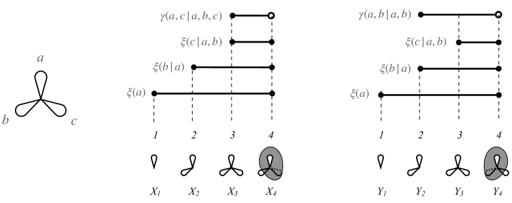
Figure 1: The saecular cokernel factors of two different filtered CW complexes, $X$ and $Y$. Each nonzero factor appears as a closed or half-open interval.

$$A^{X} =\begin{array}[]{r|ccccc|}\cline{2-6}\cr 5&0&\langle{a}\rangle&\langle{a,b}\rangle&\langle{a,b,c}\rangle&\langle{a,b,c}\rangle\\ 4&0&0&0&F&F\\ 3&0&0&0&0&0\\ 2&0&0&0&0&0\\ 1&0&0&0&0&0\\ 0&0&0&0&0&0\\ \cline{2-6}\cr\lx@intercol\hfil\hfil\lx@intercol&\lx@intercol\hfil 0\hfil\lx@intercol&\lx@intercol\hfil 1\hfil\lx@intercol&\lx@intercol\hfil 2\hfil\lx@intercol&\lx@intercol\hfil 3\hfil\lx@intercol&\lx@intercol\hfil 4\hfil\lx@intercol\\ \end{array} A^{Y} =\begin{array}[]{r|ccccc|}\cline{2-6}\cr 5&0&\langle{a}\rangle&\langle{a,b}\rangle&\langle{a,b,c}\rangle&\langle{a,b,c}\rangle\\ 4&0&0&G&G&G\\ 3&0&0&0&0&0\\ 2&0&0&0&0&0\\ 1&0&0&0&0&0\\ 0&0&0&0&0&0\\ \cline{2-6}\cr\lx@intercol\hfil\hfil\lx@intercol&\lx@intercol\hfil 0\hfil\lx@intercol&\lx@intercol\hfil 1\hfil\lx@intercol&\lx@intercol\hfil 2\hfil\lx@intercol&\lx@intercol\hfil 3\hfil\lx@intercol&\lx@intercol\hfil 4\hfil\lx@intercol\\ \end{array}$$ (21)

4 Organization

In §5 and §6 we review existing literature and introduce several notational conventions. In §7 and §8 we recall the definitions of a Puppe exact category and a free lattice homomorphism, respectively; we also prove structural properties needed for subsequent constructions. In §9 we introduce saecular decomposition for chain diagrams valued in Puppe exact categories. In §10 we adapt and extend this framework to diagrams valued in $\mathsf{Group}$. In §11, §12, and §13 we relate saecular barcodes with (classical, ${\mathds{k}}$-linear) persistence diagrams, generalized persistence diagrams, and Leray-Serre spectral sequences, respectively. In §A we review a key technical result concerning free modular lattices. In §B we prove a related result, which is used to establish existence of saecular CD homomorphisms in general, for functors from a well ordered set to $\mathsf{E}\in\{R\mathsf{Mod},\mathsf{Mod}R,\mathsf{Group}\}$. In §C we supply proofs for Theorems 1 - 8.

5 Literature

Functors valued in categories other than ${\mathds{k}}\mathsf{VectFin}$. Persistence modules valued in a category other than finite-dimensional ${\mathds{k}}$-vector spaces find diverse interesting examples in data science. The earliest examples of persistent topological structure in data include spaces with torsion, e.g. the Klein bottle [12]. The method of circular coordinates developed in [33], for example, relies explicitly on the use of integer coefficients. Persistence for circle-valued maps has also been considered by Burghelea and Dey in [8] and by Burghelea and Haller in [9].

Mendez and Sanchez-Garcia have recently explored notions of persistence for homology with semiring coefficients, motivated by applications in biology, neuroscience, and network science [32].

Work in Floer homology has recently prompted active exploration of the infinite-dimensional case. In [42], Usher and Zhang introduces persistence for Floer homology via a non-Archimedean singular value decomposition of the boundary operator of the chain complex. This work has generated a rapidly growing body of literature [36], including works on autonomous Hamiltonian flows [35] and rational curves of smooth surfaces [7].

The decomposition of integer homological persistence modules (i.e., modules obtained by applying the $n$th homology functor with $\mathbf{Z}$ coefficients to a filtered sequence of topological spaces) has been studied by Romero et al. in [40]. This treatment is closely entwined with spectral sequences, and has led to interesting directions in multi-persistence and spectral systems [39]. This approach also has several interesting algorithmic aspects. Filtrations and bifiltrations play a prominent role.

Generalized persistence. The generalized persistence diagram was introduced for $\mathbf{R}$-parametrized constructible modules valued in Krull-Schmidt categories by Patel in [34]. Patel and McClearly have recently adapted the principles introduced in this work to achieve novel stability results in multiparameter persistence [30].

Chain functors, lattices, and exact categories. The theory of Puppe exact categories has an expansive treatment in [24] and other works by M. Grandis. Of particular relevance, [24] concretely describes the universal RE model and p-exact classifying category for an $\mathbf{I}$-indexed diagram in $E$, where $\mathbf{I}$ is any totally ordered set and $\mathsf{E}$ is any exact category [24]. One of only a few technical challenges to relating this work with interval decomposition of persistence modules can be summarized as extending this construction from free lattice homomorphisms to free complete lattice homomorphisms; the present work expand and addresses this challenge in detail. The Puppe exact category of partial matchings has also appeared in the literature of persistence, specifically with regard to stability cf. [3].

Order lattices. The lattice-theoretic approach to persistence presented in this work was previewed by an analogous matroid theoretic treatment in [25] and [26]. Lattice theoretic structure in persistence modules has also been explored in [15] and [16]. More broadly, the description of persistence in terms of the fundamental subspaces (kernel and image) has been a recurring theme since the emergence of the field. The basics of this analysis appear in the seminal works of Robins [38], Edelsbrunner, Letscher, and Zomorodian [19]; as well as in Carlsson and Zomorodian [43] which reformulates the persistence diagram in terms of graded modules. Bifiltrations play a central role in the reformulation of Carlsson and de Silva [10] and in diverse other works.

Persistent homotopy. The notion of a persistent homotopy group was introduced by Letscher [29], as a tool to study knotted complexes which become unknotted under inclusion into larger spaces. The definition of a persistent homotopy group, in this work, has a natural analog to that of a persistent homology group. The family of all such groups corresponds conceptually to what Patel [34] terms the rank function, rather than a persistence diagram or barcode. Letscher’s treatment is formally disjoint from that of Patel, for several reasons; first, it includes homotopy in dimension 1, which does not fit into an abelian category; second, persistent homotopy groups are subquotients of loop spaces in which class representatives are well-defined – this level of details is abstracted away in generalized PD’s; third and finally, Letscher does not define a persistence diagram or barcode to complement the notion of a persistent homotopy group. More recently, Mémoli and Zhou [31] have explored several possible notions of persistent homotopy for metric spaces.

In [5], Blumberg and Lesnick show that interleavings form a universal pseudometric on persistent homotopy groups (unlike [29], these authors use the term persistent homotopy group to refer to any functor obtained by composing a functor $\mathbf{R}\to\mathsf{Top}$ with a homotopy functor $\pi_{n}$). Several useful and fundamental properties of persistent homotopy are explored in [2]. Further properties of persistent homotopy have been explored in [28].

Spectral sequences Connections between persistence and spectral sequences have been suggested essentially since the formalization of persistent homology as a concept [20, 17]. A formal relation between the two was introduced in [1]. Revisions and extensions of this relationship to integral homology are discussed in [40], though we do not know a refereed reference for this discussion as of yet.

6 Definitions

We assume working familiarity with the definitions of poset, order lattice, and lattice homomorphism. Definitions for complete, completely distributive (CD), modular, and algebraic lattices can be found in standard references. As certain terms in order theory have distinct but related definitions elsewhere, however, there are several points with real risk of confusion. We endeavor to indicate these cases as they arise, and, where necessary, to disambiguate by introducing nonstandard variants of the standard terms.

Partially ordered sets. For economy of notation, $\mathrm{P}$ will denote both a poset and the associated posetal category. The dual poset $\mathrm{P}^{*}$ represents the dual poset and the opposite category $\mathrm{P}{{}^{\mathrm{op}}}$. The partial order on $\mathrm{P}$ is denoted $\mathrm{Rel}(\mathrm{P})$, and the set of covering relations is ${\mathrm{Cov}}(\mathrm{P})\subseteq\mathrm{Rel}(\mathrm{P})$. Given $a\in\mathrm{P}$, we write

$$\downarrow_{\mathrm{P}}a =\{b\in\mathrm{P}:b\leq a\} \mathring{\downarrow}_{\mathrm{P}}a=\{b\in\mathrm{P}:b<a\}$$

$$\uparrow_{\mathrm{P}}a =\{b\in\mathrm{P}:b\geq a\} \mathring{\uparrow}_{\mathrm{P}}a=\{b\in\mathrm{P}:b>a\}$$

We omit subscripts on arrows where context leaves no room for confusion.

The maximum of $\mathrm{P}$, should such an element exist, is denoted $1_{\mathrm{P}}$ or $1$. The minimum element is denoted $0_{\mathrm{P}}$ or $0$. A poset with both minimum and maximum is bounded. A poset homomorphism $f:\mathrm{P}\to\mathrm{Q}$ preserves existing maxima if $\mathrm{P}=\downarrow p$ implies $\mathrm{Q}=\downarrow f_{p}$. Preservation of existing minima (respectively, existing bounds) is defined similarly. A bound-preserving poset homomorphism with a bounded domain and codomain is called bounded.

Unless otherwise indicated, $\mathrm{P}\times\mathrm{Q}$ denotes the canonical realization of the product of $\mathrm{P}$ and $\mathrm{Q}$ in the category of posets and order-preserving maps. Concretely, if $\mathrm{Grs}(\mathrm{P})$ denotes the ground set of $\mathrm{P}$, then

$$\mathrm{Grs}(\mathrm{P}\times\mathrm{Q})=\mathrm{Grs}(\mathrm{P})\times\mathrm{Grs}(\mathrm{Q})$$

and $(a^{\prime},b^{\prime})\leq(a,b)$ iff $a^{\prime}\leq a$ and $b^{\prime}\leq b$. The $m$-fold product of $\mathrm{P}$ with itself is $\mathrm{P}^{m}$. An interval in $\mathrm{P}$ is a subset ${I}\subseteq\mathrm{P}$ such that $a,b\in{I}$ and $a\leq x\leq b$ implies $x\in{I}$. The family of intervals is denoted ${\mathbb{I}}(\mathrm{P})$. Given $a,b\in\mathrm{P}$, we write $[a,b]$ for the interval $\{p\in\mathrm{P}:a\leq p\leq b\}$.

We will often wish to work with both a poset $\mathrm{P}$ and a copy of $\mathrm{P}$, whose elements are disjoint from, but nevertheless comparable to, the elements of $\mathrm{P}$. We achieve this by defining $\hat{\mathrm{P}}=\mathrm{P}\times\{0\}$, the product of $\mathrm{P}$ with a 1-element poset. We have $\mathrm{P}\cap\hat{\mathrm{P}}=\emptyset$, but there exists a canonical isomorphism $\pi:\hat{\mathrm{P}}\to\mathrm{P},\;(p,0)\mapsto p$. Moreover, we can compare elements of $\hat{\mathrm{P}}$ to those of $\mathrm{P}$ by defining a binary relation (not a partial order) $\preceq$ such that $\hat{p}\preceq p$ iff $\pi(\hat{p})\leq p$, for each $\hat{p}\in\hat{\mathrm{P}}$ and $p\in\mathrm{P}$.

Relations. Given sets $S$, $T$ and a binary relation $\sim$ contained in $S\times T$, we write

$$S_{\sim t}:=\{s\in S:s\sim t\}$$

for each $t\in T$. Similarly, given any function $f:U\to S$, we write $f_{\sim t}:=\{u\in U:f(u)\sim t\}.$ so that, for example,

$$\mathbf{N}=\uparrow_{\mathbf{Z}}0=\mathbf{Z}_{\geq 0}.$$

Complete lattices and homomorphisms. A set function $f:\mathbf{L}\to\mathbf{Q}$ preserves existing (nonempty) suprema if $\bigvee f(S)$ exists and satisfies $\bigvee f(S)=f(\bigvee S)$ for each (nonempty) $S\subseteq\mathbf{L}$ such that $\bigvee S$ exists. Preservation of existing (nonempty) infima is defined similarly.

A lattice $\mathbf{L}$ is complete if $\bigvee S$ and $\bigwedge S$ exist for each $S\subseteq\mathbf{L}$. A lattice homomorphism $f$ is

• $\exists$-complete if $f$ preserves existing suprema and infima

• $\mathring{\exists}$-complete if $f$ preserves existing nonempty suprema and infima

• $\forall$-complete if $f$ preserves existing suprema and infima, and has a complete domain

• $\mathring{\forall}$-complete if $f$ preserves existing nonempty suprema and infima, and has a complete domain

• complete if $f$ preserves existing suprema and infima, and has a complete domain and codomain

A sublattice $\mathbf{Q}\subseteq\mathbf{L}$ is $\exists$-complete if the inclusion $\mathbf{Q}\subseteq\mathbf{L}$ is $\exists$-complete. The same convention applies to all other notions of completeness listed above.

Upper and lower continuity. A lattice is upper continuous or meet continuous if for any $a\in\mathbf{L}$ the poset homomorphism $x\mapsto x\wedge a$ preserves upward directed suprema [maeda2012theory]. It is lower continuous or join continuous if $\mathbf{L}^{*}$ is meet continuous; that is, if for any $a\in\mathbf{L}$ the poset homomorphism $x\mapsto x\vee a$ preserves downward directed infima.

Set rings. It will be convenient to assign a fixed notation to several set rings associated to a partially ordered set $\mathrm{P}$. In particular, we define the following.

${\mathbb{P}}(\mathrm{P})$

the power set lattice on the ground set of $\mathrm{P}$

${\mathbb{A}(\mathrm{P})}$

the lattice of decreasing subsets of $\mathrm{P}$. Equivalently, the complete set ring of Alexandrov closed subsets of $\mathrm{P}$.

$\mathbb{\mathring{A}}(\mathrm{P})$

the lattice of proper nonempty decreasing subsets of $\mathrm{P}$

${\mathbb{S}(\mathrm{P})}$

the minimum sublattice of ${\mathbb{A}(\mathrm{P})}$ containing $\{\;{\downarrow}\;p:p\in\mathrm{P}\}$. Unlike the preceding examples, this object is in general only a semitopology.

These operations may be composed. For example, the complete lattice $\mathbb{A}^{2}(\mathrm{P})=\mathbb{A}(\mathbb{A}(\mathrm{P}))$ of decreasing sets of decreasing sets will play a central role in the following story.

Free embeddings. Given $\mathbb{X}\in\{\mathbb{A},\mathbb{\mathring{A}}\}$, the free embedding $\mu:\mathrm{P}\to\mathbb{A}\mathbb{X}(\mathrm{P})$ is the map such that

$$\mu(p)=\{T\in\mathbb{X}(\mathrm{P}):p\notin T\}$$

for each $p\in\mathrm{P}$. The term free is justified in this context by Theorem 19 (Tunnicliffe [41]). Some useful facts about free embeddings follow directly from the definition:

1. If $\mathbb{X}=\mathbb{A}$, then $\mu(p)={\mathbb{A}(\mathrm{P}-\uparrow p)}$.

2. The free embedding fails to preserve suprema and infima, in general.

3. The free embedding preserves existing maxima (respectively, minima) iff $\mathbb{X}=\mathbb{\mathring{A}}$.

Order chains. The term chain is synonymous with totally ordered set in classical order theory. A chain in $X$ means a totally ordered subset of $X$. The notions of boundedness and completeness which we have introduced for posets and lattices are also suitable for every chain, when regarded as an order lattice. Thus a $\mathring{\forall}$-complete chain in $\mathbf{L}$ is a $\mathring{\forall}$-complete sublattice of $\mathbf{L}$ that is totally ordered as a poset, a bounded chain in $\mathrm{P}$ is a totally ordered subset containing maximum and minimum, etc.

Chain functors. A chain functor in a category $\mathsf{E}$ is a functor of form $f:\mathbf{I}\to\mathsf{E}$ for some chain $\mathbf{I}$. When $\mathsf{E}$ has a zero object, the support of $f$ can be defined

$$\mathrm{supp}(f):=\{i\in\mathbf{I}:f_{i}\neq 0\}.$$

A functor has support type $S$ if $\mathrm{supp}(f)\in\{S,\emptyset\}$. In particular, the 0 functor has every support type.

A chain functor is interval if

$$f(i\leq j)\quad\text{is}\quad\begin{cases}\text{invertible}&i,j\in\mathrm{supp}(f)\\ \text{zero}&else.\end{cases}$$

The support of every interval chain functor is an interval of $\mathbf{I}$. The object type of a nonzero interval functor is the isomorphism class $f_{i}$, where $i$ is any element of $\mathrm{supp}(f)$. The object type of the zero functor is the isomorphism class of the zero object.

Categories. We write $\mathsf{CD}$ for the category of completely distributive lattices and complete lattice homomorphisms, and $\mathsf{P}$ for the category of partially ordered sets and order-preserving functions. The category of sets and functions is $\mathsf{Set}$, and the category of pointed sets is $\mathsf{SetP}$. The category of groups and group homomorphisms is $\mathsf{Group}$. The category of vector spaces and finite-dimensional vector spaces over ${\mathds{k}}$ are denoted ${\mathds{k}}\mathsf{Vect}$ and ${\mathds{k}}\mathsf{VectFin}$, respectively.

7 P-exact categories

Puppe exact categories are generalizations of abelian categories that may or may not be additive. Formally, a well-powered category $\mathsf{C}$ is Puppe exact (or p-exact) if (i) it has a zero object, kernels, and cokernels, (ii) every mono is a kernel and every epi is a cokernel, (iii) every morphism has an epi-mono factorization. Here we review the definitions and prove some basic structural results used in later sections. The reader is referred to [24] for further details.

7.1 First principles

Let $\mathsf{E}$ be a p-exact category. The direct and inverse image operators of an arrow $f:A\to B$ are denoted

$$f_{\,\begin{picture}(1.0,1.0)(-1.0,-2.0)\circle*{2.0}\end{picture}\ }:\mathrm{Sub}(A)\to\mathrm{Sub}(B) f^{\,\begin{picture}(1.0,1.0)(-1.0,-2.0)\circle*{2.0}\end{picture}\ }:\mathrm{Sub}(B)\to\mathrm{Sub}(A)$$

respectively.

Proposition 9 (Grandis, [24, p. 48-52]).

Let $f:A\to B$ be an arbitrary arrow in $\mathsf{E}$.

1. The poset $\mathrm{Sub}(A)$ is a modular lattice.

2. The pair $(f_{\,\begin{picture}(1.0,1.0)(-1.0,-2.0)\circle*{2.0}\end{picture}\ },f^{\,\begin{picture}(1.0,1.0)(-1.0,-2.0)\circle*{2.0}\end{picture}\ })$ is a modular connection. Concretely, this means that $f_{\,\begin{picture}(1.0,1.0)(-1.0,-2.0)\circle*{2.0}\end{picture}\ }$ and $f^{\,\begin{picture}(1.0,1.0)(-1.0,-2.0)\circle*{2.0}\end{picture}\ }$ preserve order, and

   $$f^{\,\begin{picture}(1.0,1.0)(-1.0,-2.0)\circle*{2.0}\end{picture}\ }f_{\,\begin{picture}(1.0,1.0)(-1.0,-2.0)\circle*{2.0}\end{picture}\ }(a)=a\vee f^{\,\begin{picture}(1.0,1.0)(-1.0,-2.0)\circle*{2.0}\end{picture}\ }(0) f_{\,\begin{picture}(1.0,1.0)(-1.0,-2.0)\circle*{2.0}\end{picture}\ }f^{\,\begin{picture}(1.0,1.0)(-1.0,-2.0)\circle*{2.0}\end{picture}\ }(b)=b\wedge f_{\,\begin{picture}(1.0,1.0)(-1.0,-2.0)\circle*{2.0}\end{picture}\ }(1)$$

   for all $a\in\mathrm{Sub}(A)$ and all $b\in\mathrm{Sub}(B)$. In particular, $(f_{\,\begin{picture}(1.0,1.0)(-1.0,-2.0)\circle*{2.0}\end{picture}\ },f^{\,\begin{picture}(1.0,1.0)(-1.0,-2.0)\circle*{2.0}\end{picture}\ })$ is a Galois connection.

3. Consequently, if $S\subseteq\mathrm{Sub}(A)$ and $\bigvee S$ exists, then $\bigvee(f_{\,\begin{picture}(1.0,1.0)(-1.0,-2.0)\circle*{2.0}\end{picture}\ }S)$ exists, and $f_{\,\begin{picture}(1.0,1.0)(-1.0,-2.0)\circle*{2.0}\end{picture}\ }(\bigvee S)=\bigvee f_{\,\begin{picture}(1.0,1.0)(-1.0,-2.0)\circle*{2.0}\end{picture}\ }(S)$. Dually $f^{\,\begin{picture}(1.0,1.0)(-1.0,-2.0)\circle*{2.0}\end{picture}\ }(\bigwedge S)=\bigwedge f^{\,\begin{picture}(1.0,1.0)(-1.0,-2.0)\circle*{2.0}\end{picture}\ }(S)$ for any $S$ such that $\bigwedge S$ exists.

The family of bounded modular lattices and modular connections forms a p-exact category under the composition rule $(g_{\,\begin{picture}(1.0,1.0)(-1.0,-2.0)\circle*{2.0}\end{picture}\ },g^{\,\begin{picture}(1.0,1.0)(-1.0,-2.0)\circle*{2.0}\end{picture}\ })\circ(f_{\,\begin{picture}(1.0,1.0)(-1.0,-2.0)\circle*{2.0}\end{picture}\ },f^{\,\begin{picture}(1.0,1.0)(-1.0,-2.0)\circle*{2.0}\end{picture}\ }):=(g_{\,\begin{picture}(1.0,1.0)(-1.0,-2.0)\circle*{2.0}\end{picture}\ }f_{\,\begin{picture}(1.0,1.0)(-1.0,-2.0)\circle*{2.0}\end{picture}\ },f^{\,\begin{picture}(1.0,1.0)(-1.0,-2.0)\circle*{2.0}\end{picture}\ }g^{\,\begin{picture}(1.0,1.0)(-1.0,-2.0)\circle*{2.0}\end{picture}\ }).$ We denote this category $\mathrm{Mlc}$, and denote the full subcategory of complete modular lattices by $\mathrm{CMlc}$. If one defines $\mathrm{Sub}(f)$ to be the direct/inverse image pair $(f_{\,\begin{picture}(1.0,1.0)(-1.0,-2.0)\circle*{2.0}\end{picture}\ },f^{\,\begin{picture}(1.0,1.0)(-1.0,-2.0)\circle*{2.0}\end{picture}\ })$ for each arrow $f$ in a Puppe exact category $\mathsf{E}$, then $\mathrm{Sub}$ is an (exact) functor $\mathsf{E}\to\mathrm{Mlc}$. For details see [24].

Each arrow $f:A\to B$ in $\mathrm{Mlc}$ admits a unique epi-mono factorization of form

where

$$q_{\,\begin{picture}(1.0,1.0)(-1.0,-2.0)\circle*{2.0}\end{picture}\ }(x) =x\vee f^{\,\begin{picture}(1.0,1.0)(-1.0,-2.0)\circle*{2.0}\end{picture}\ }0 n_{\,\begin{picture}(1.0,1.0)(-1.0,-2.0)\circle*{2.0}\end{picture}\ }(y)=y g_{\,\begin{picture}(1.0,1.0)(-1.0,-2.0)\circle*{2.0}\end{picture}\ }(x)=f_{\,\begin{picture}(1.0,1.0)(-1.0,-2.0)\circle*{2.0}\end{picture}\ }(x)$$

$$q^{\,\begin{picture}(1.0,1.0)(-1.0,-2.0)\circle*{2.0}\end{picture}\ }(x) =x n^{\,\begin{picture}(1.0,1.0)(-1.0,-2.0)\circle*{2.0}\end{picture}\ }(y)=y\wedge f_{\,\begin{picture}(1.0,1.0)(-1.0,-2.0)\circle*{2.0}\end{picture}\ }1 g^{\,\begin{picture}(1.0,1.0)(-1.0,-2.0)\circle*{2.0}\end{picture}\ }(y)=f^{\,\begin{picture}(1.0,1.0)(-1.0,-2.0)\circle*{2.0}\end{picture}\ }(y)$$

Each subobject of $\mathbf{L}$, regarded as subobject in either $\mathrm{Mlc}$ of $\mathrm{CMlc}$, engenders a unique mono of form

$$(f_{\,\begin{picture}(1.0,1.0)(-1.0,-2.0)\circle*{2.0}\end{picture}\ },f^{\,\begin{picture}(1.0,1.0)(-1.0,-2.0)\circle*{2.0}\end{picture}\ }):[0,a]_{\mathbf{L}}\to\mathbf{L} f_{\,\begin{picture}(1.0,1.0)(-1.0,-2.0)\circle*{2.0}\end{picture}\ }b=b f^{\,\begin{picture}(1.0,1.0)(-1.0,-2.0)\circle*{2.0}\end{picture}\ }b=a\wedge b.$$

Thus subobjects of $\mathbf{L}$ are in canonical 1-1 correspondence with elements of $\mathbf{L}$, and, equivalently, with intervals of form $[0,a]_{\mathbf{L}}$. A similar correspondence holds between quotients of $\mathbf{L}$, connections of form $(f_{\,\begin{picture}(1.0,1.0)(-1.0,-2.0)\circle*{2.0}\end{picture}\ },f^{\,\begin{picture}(1.0,1.0)(-1.0,-2.0)\circle*{2.0}\end{picture}\ }):\mathbf{L}\to[a,1]$, where $f^{\,\begin{picture}(1.0,1.0)(-1.0,-2.0)\circle*{2.0}\end{picture}\ }$ is inclusion and $f_{\,\begin{picture}(1.0,1.0)(-1.0,-2.0)\circle*{2.0}\end{picture}\ }(b)=a\vee b$, elements of $\mathbf{L}$, and intervals of form $[a,1]_{\mathbf{L}}$.

Lemma 10.

The direct image operator of an arrow $f:A\to B$ restricts to a complete lattice homomorphism on each $\forall$-complete CD sublattice of $\mathrm{Sub}(A)$ containing the kernel of $f$. The dual statement holds for inverse image operator. Similarly, the direct image operator of an arrow $f:A\to B$ restricts to a lattice homomorphism on each distributive sublattice of $\mathrm{Sub}(A)$ containing the kernel of $f$. The dual statement holds for inverse image operator.

Proof.

Let $\mathbf{L}$ be a $\forall$-complete CD sublattice of $\mathrm{Sub}(A)$ that contains $k:=\mathrm{ker}(f)$, and fix $S\subseteq\mathbf{L}$. Complete distributivity then provides the third of the following identities

$$\textstyle f_{\,\begin{picture}(1.0,1.0)(-1.0,-2.0)\circle*{2.0}\end{picture}\ }(\bigwedge S)=f_{\,\begin{picture}(1.0,1.0)(-1.0,-2.0)\circle*{2.0}\end{picture}\ }(f^{\,\begin{picture}(1.0,1.0)(-1.0,-2.0)\circle*{2.0}\end{picture}\ }f_{\,\begin{picture}(1.0,1.0)(-1.0,-2.0)\circle*{2.0}\end{picture}\ }\bigwedge S)=f_{\,\begin{picture}(1.0,1.0)(-1.0,-2.0)\circle*{2.0}\end{picture}\ }((\bigwedge S)\vee k)=f_{\,\begin{picture}(1.0,1.0)(-1.0,-2.0)\circle*{2.0}\end{picture}\ }(\bigwedge\{s\vee k:s\in S\})=\\ \textstyle f_{\,\begin{picture}(1.0,1.0)(-1.0,-2.0)\circle*{2.0}\end{picture}\ }(\bigwedge\{f^{\,\begin{picture}(1.0,1.0)(-1.0,-2.0)\circle*{2.0}\end{picture}\ }f_{\,\begin{picture}(1.0,1.0)(-1.0,-2.0)\circle*{2.0}\end{picture}\ }s:s\in S\})=f_{\,\begin{picture}(1.0,1.0)(-1.0,-2.0)\circle*{2.0}\end{picture}\ }(f^{\,\begin{picture}(1.0,1.0)(-1.0,-2.0)\circle*{2.0}\end{picture}\ }\bigwedge\{f_{\,\begin{picture}(1.0,1.0)(-1.0,-2.0)\circle*{2.0}\end{picture}\ }s:s\in S\})=\bigwedge f_{\,\begin{picture}(1.0,1.0)(-1.0,-2.0)\circle*{2.0}\end{picture}\ }(S).$$

This establishes the claim for the direct image operator, since $f_{\,\begin{picture}(1.0,1.0)(-1.0,-2.0)\circle*{2.0}\end{picture}\ }$ preserves existing joins. The claim for inverse image is equivalent, by duality. If we assume, instead, that $\mathbf{L}$ is distributive, then similar argument shows the direct and inverse image operators preserve binary meets and joins. ∎

Given any index category $\mathsf{I}$, we denote the category of $\mathsf{I}$-shaped diagrams in $\mathsf{E}$ by $[\mathsf{I},\mathsf{E}]$. Diagrams make new p-exact categories from old.

Lemma 11 (P-exact diagrams).

Let $\mathsf{I}$ be a small category.

1. The category of diagrams $[\mathsf{I},\mathsf{E}]$ is p-exact.

2. Kernels and cokernels obtain object-wise. Concretely, $0\rightarrow A\xrightarrow{m}B\xrightarrow{p}C\rightarrow 0$ is exact in $[\mathsf{I},\mathsf{E}]$ if and only if $0\rightarrow A_{i}\xrightarrow{m_{i}}B_{i}\xrightarrow{p_{i}}C_{i}\rightarrow 0$ is exact in $\mathsf{E}$, for each $i$.

3. An arrow $A\xrightarrow{m}B$ in $[\mathsf{I},\mathsf{E}]$ is mono iff $m_{i}$ is mono for each $i$. Likewise for epis.

4. If $(B^{j})_{j\in J}$ is an indexed family of subdiagrams of $A$ and $\bigvee_{j}B^{j}_{i}$ exists for each $i$, then $\bigvee B$ exists and obtains object-wise. The dual statement holds for meets.

Proof.

Claim 1 is a routine exercise, as observed in [24, p. 48]. Coincidence of exact and object-wise exact sequences follows from the universal property of (co)kernels. Claim 3 follows Claim 2, since p-exact categories have normal epis and monos [24, p. 46]. Claim 4 follows Claim 3. ∎

7.2 Regular and canonical induction

If $\mathsf{C}$ is any category with subobjects and $A$ is an object in $\mathsf{C}$, then we may define a poset $\mathrm{P}(A)$ such that $\mathrm{Grs}(\mathrm{P}(A))=\{(M,N)\in\mathrm{Sub}(A)^{2}:M\leq N\leq A\}$, ordered such that $(M,N)\leq(M^{\prime},N^{\prime})$ iff $N\leq N^{\prime}$ and $M\leq M^{\prime}$. We say that $(M,N)\leq(M^{\prime},N^{\prime})$ is a doubly nested pair, and call $\mathrm{P}(A)$ the poset of nested pairs in $A$. We call the corresponding homomorphism $N/M\to N^{\prime}/M^{\prime}$ the regularly induced map, cf. [24]. The following lemma can be proved directly using the axioms of kernels and cokernels.

Lemma 12.

Regularly induced maps are closed under composition. More precisely, for each object $A$ in $\mathsf{E}$ there exists a functor $\mathsf{F}:\mathrm{P}(A)\to\mathsf{E}$ sending ${(M,N)}$ to $N/M$ and sending each relation $(M,N)\leq(M^{\prime},N^{\prime})$ to the regularly induced map $N/M\to N^{\prime}/M^{\prime}$.

Following [24], let us define a binary relation $\Phi_{\mathsf{M}}$ on the family of subquotients of $A$ such that

$$N/M\;\Phi_{\mathsf{M}}\;N^{\prime}/M^{\prime} \iff M\vee N^{\prime}=N\vee M^{\prime}\quad\text{and}\quad M\wedge N^{\prime}=M^{\prime}\wedge N.$$ (22)

Remark 5.

Grandis defines this relation, mutual domination, in a rather more general context than that which we require here. Equivalence between (22) and this more abstract formulation appears in expression (4.3.2) of [24], and a more accessible interpretation appears in the proof of Theorem 4.3.5.

Lemma 13.

Suppose that $M\subseteq N$ and $M^{\prime}\subseteq N^{\prime}$ are elements of the lattice $\mathbf{L}$ of closed sets in a semitopology. Then

$$N/M\;\Phi_{\mathsf{M}}\;N^{\prime}/M^{\prime}\quad\iff\quad N-M=N^{\prime}-M^{\prime}$$

Proof.

If $N-M=N^{\prime}-M^{\prime}$ then $N\vee N^{\prime}=N\vee M^{\prime}=M\vee N^{\prime}$ and $M\wedge M^{\prime}=M\wedge N^{\prime}=M^{\prime}\wedge N$. The converse holds by a similar set theoretic argument; see the note following Lemma 1.2.6 in [24, p. 23]. ∎

Theorem 14 (Induced isomorphisms [24]).

If $A$ is an object in $\mathsf{E}$ and $N,N^{\prime}\in\mathrm{Sub}(A)$, then the map $\phi$ defined by commutativity of

(23)

is an isomorphism. Moreover, if $N/M\;\Phi_{\mathsf{M}}\;N^{\prime}/M^{\prime}$ then there exists a commutative diagram of isomorphisms

(24)

where each solid arrow is derived as in (23).

Proof.

These results appear in [24], Lemma 2.2.9 and Proposition 4.3.6. ∎

Definition 6.

The maps $\phi$ and $\psi$ defined in (23) and (24) are Noether isomorphisms of the first and second kind, respectively. The latter may also be termed the canonical or canonically induced isomorphism.

Theorem 15 (Cohesion of canonically induced isomorphisms [24]).

Let $A$ be an object in $\mathsf{E}$ and $\mathbf{L}$ be a distributive sublattice of $\mathrm{Sub}(A)$. Then the family of canonically induced isomorphisms between subquotients with numerator and denomenator in $\mathbf{L}$ is closed under composition.

Proof.

Grandis [24, pp. 23-24, Theorem 1.2.7] proves both the stated result and its converse in the special case where $\mathsf{E}$ is the category of abelian groups. However, the same argument carries over verbatim for any p-exact category, if we use Theorem 14 to “stand in” as a generalized version of the diagram [24, p. 20, (1.16)] used in that argument. ∎

Theorem 16 (Compatibility of canonical isomorphisms with regular induction [24, p180, Theorem 4.3.7] ).

Let $(M,N)\leq(M^{\prime},N^{\prime})$ and $(P,Q)\leq(P^{\prime},Q^{\prime})$ be doubly nested pairs. Let $A_{{N}/{M}}$ and $A_{{N^{\prime}}/{M^{\prime}}}$ be objects in $\mathsf{E}$ that realize the quotients $N/M$ and $N^{\prime}/M^{\prime}$, respectively, and define $B_{Q/P}$ and $B_{Q^{\prime}/P^{\prime}}$ similarly.

If $N/M\;\Phi_{\mathsf{M}}\;Q/P$ and $N^{\prime}/M^{\prime}\;\Phi_{\mathsf{M}}\;Q^{\prime}/P^{\prime}$, then the following diagram commutes, where horizontal arrows are regularly induced maps and vertical arrows are canonically induced isomorphisms.

(25)

Remark 6.

Theorem 16 intentionally avoids the conventional abuse of notation that conflates $N/M$ with a representative of a cokernel in $\mathsf{E}$. Note, in particular, even when $(M,N)=(M^{\prime},N^{\prime})$ and $(P,Q)=(P^{\prime},Q^{\prime})$, it is possible that $A_{N/M}\neq B_{Q/P}$. Thus, in particular, Theorem 16 says something nontrivial about the relationship between regularly induced maps and the isomorphisms that exist (via the universal property of cokernels) between distinct representatives of a cokernel.

A quasi-regular induction on a sublattice $\mathbf{L}\subseteq\mathrm{Sub}_{A}$ is a commutative square of form

(26)

where the numerator and denominator of each subquotient lie in $\mathbf{L}$, vertical arrows are canonically induced isomorphisms (in particular $N/M\Phi_{\mathsf{M}}N^{\prime}/M^{\prime}$ and $Q/P\Phi_{\mathsf{M}}Q^{\prime}/P^{\prime}$) and the lower horizontal arrow is regularly induced. In this case we say that $f$ is $\mathbf{L}$-quasi-regularly induced, and write $f:(N,M,Q,P)\sim(N^{\prime},M^{\prime},Q^{\prime},P^{\prime})$.

Lemma 17.

If $\mathbf{L}$ is a distributive sublattice of $\mathrm{Sub}(A)$ and $N\leq M$ and $Q\leq P$ are nested pairs in $\mathbf{L}$, then there exists at most one $\mathbf{L}$-quasi-regularly induced arrow $N/M\to Q/P$.

Proof.

Suppose that $f:(N,M,Q,P)\sim(N^{\prime},M^{\prime},Q^{\prime},P^{\prime})$ and $f:(N,M,Q,P)\sim(N^{\prime\prime},M^{\prime\prime},Q^{\prime\prime},P^{\prime\prime})$. Then we have a diagram of regularly induced maps (solid) and canonically induced isomorphisms (dashed)

(27)

Each triangle of dashed arrows in (29) commutes by distributive cohesion (Theorem 15). The bottom face, composed of two parallel solid arrows and two parallel dashed arrows, commutes by Theorem 16. Thus any dotted arrow $f$ that makes the back face commute also makes the slanted face commute, and vice versa. ∎

7.3 Exact functors via lattice homomorphisms

Let $\mathbf{L}$ be the lattice of closed sets in a semitopological space $X$. Let $\Lambda:\mathbf{L}\to\mathrm{Sub}_{A}$ be a bound-preserving lattice homomorphism from $\mathbf{L}$ to the subobject lattice of an object $A$ in a p-exact category $\mathsf{E}$.

The main result of this section is Theorem 18. This closely resembles (and may be subsumed by) several existing results in [24]. We give a proof which is completely elementary, and which can be modified to work outside the the setting of p-exact categories, which we will do in later sections.

Theorem 18.

There exists an exact functor

$${\Omega}:\mathrm{Lcl}(\mathbf{L})\to\mathsf{E}$$

which agrees with $\Lambda$ on $\mathbf{L}$, in the sense that ${\Omega}|_{\mathbf{L}}=\Lambda.$

If ${\Omega}^{\prime}$ is any other functor satisfying the same criterion, then there exists a unique natural isomorphism $\eta:{\Omega}\cong{\Omega}^{\prime}$ such that $\eta|_{\mathbf{L}}$ is identity. Transformation $\eta$ assigns the canonically induced isomorphism $\eta_{A/B}:{\Omega}_{A/B}\cong{\Omega}^{\prime}_{A/B}$ to each nested pair $B\leq A\in\mathbf{L}$.

Proof.

We will construct ${\Omega}$ directly. To reduce notation, write $|S|$ for $\Lambda S$. Invoking the axiom of choice if necessary, for each object $A\in\mathrm{Lcl}(\mathbf{L})$ select a nested pair $M_{A}\leq N_{A}\in\mathbf{L}$ such that $A=N_{A}-M_{A}$, and define ${\Omega}A=\frac{|N_{A}|}{|M_{A}|}$.

For each regularly induced map $f:B\to B^{\prime}$ in $\mathrm{Lcl}(\mathbf{L})$, select a doubly nested pair $(M,N)\leq(M^{\prime},N^{\prime})$ such that $A=N-M$ and $A^{\prime}=N^{\prime}-M^{\prime}$. Let ${\Omega}f$ be the unique map such that the following diagram commutes, where vertical arrows are canonically induced isomorphisms; such isomorphisms exist by Lemma 13 and Theorem 14.

(28)

Claim 1. Every choice of of doubly nested pair $(M,N)\leq(M^{\prime},N^{\prime})$ yields the same value for ${\Omega}f$. Proof. Map ${\Omega}f$ is quasi-regularly induced on $\mathrm{Im}(\Lambda)$; uniqueness follows from Lemma 17.

Claim 2. Function ${\Omega}$ preserves composition of regularly induced maps. More precisely, if $f,g,h$ are regularly induced maps such that $h=gf$, then ${\Omega}h=({\Omega}g)({\Omega}f)$. Proof. Select doubly nested pairs $(M,N)\leq(M^{\prime},N^{\prime})$ and $(M^{\prime},N^{\prime})\leq(M^{\prime\prime},N^{\prime\prime})$ for $f$ and $g$. Then $(M,N)\leq(M^{\prime\prime},N^{\prime\prime})$ is a doubly nested pair for $h$. Then we have a diagram of for (29), with regularly induced arrows (solid, lefthand side), arrows determined by ${\Omega}$ (solid, righthand side) and canonically induced isomorphisms (dashed).

(29)

The triangle on the lefthand side of (29) commutes by Lemma 12. The three rectangular faces of (29) by Claim 1. Thus the entire diagram commutes. The desired conclusion follows.

We have now defined ${\Omega}$ on regularly induced maps, a family which includes all epis and monos. To each map $h$ in $\mathrm{Lcl}(\mathbf{L})$ corresponds a unique epi-mono decomposition $h=gf$, so we may define a new function ${\Omega}^{\prime}$ on arbitrary maps via ${\Omega}^{\prime}h=({\Omega}^{\prime}g)({\Omega}^{\prime}f)$. In fact, ${\Omega}^{\prime}$ agrees with ${\Omega}$ on regularly induced maps by Claim 2, so we may simply extend the domain of definition of ${\Omega}$ to include all morphisms, via ${\Omega}^{\prime}$.

Claim 3. Function ${\Omega}$ is a functor. Proof. It suffices to show that ${\Omega}$ preserves composition of morphisms. Fix arrows

$$x =ba:M/N\to P/Q$$

$$y =dc:P/Q\to S/T$$

where $a$, $c$ are epi and $b$, $d$ are mono. Diagram (30) is then uniquely determined by commutativity and the condition that $fe$ be an epi-mono decomposition.

(30)

Each arrow in diagram (30) is regularly induced, so the diagram commutes by Claim 2. It follows that ${\Omega}(yx)=({\Omega}y)({\Omega}x)$, since $hg$ is the epi-mono decomposition of $yx$.

Claim 4. Functor ${\Omega}$ is exact. That is, ${\Omega}$ preserves short exact sequences. Proof. Fix a short exact sequence $0\to A\xrightarrow{f}B\xrightarrow{g}C\to 0$ in $\mathrm{Lcl}(\mathbf{L})$. Then there exist nested pairs $(M,N^{\prime})\leq(M,N)\leq(N^{\prime},N)$ such that the following diagram commutes, where vertical arrows are canonically induced isomorphisms

(31)

This concludes the proof that a suitable exact functor ${\Omega}$ exists. Now posit a second functor ${\Omega}^{\prime}$ with the same properties. We must show that the map $\eta$ defined in the theorem statement is a natural isomorphism ${\Omega}\cong{\Omega}^{\prime}$, and that $\eta=\eta^{\prime}$ for any natural isomorphism $\eta^{\prime}$ such that $\eta^{\prime}_{S}=1$ for each $S\in\mathbf{L}$.

To verify that $\eta$ is a natural transformation, fix a doubly nested pair $(M,N)\leq(M^{\prime},N^{\prime})$. Since ${\Omega}(N/M)\Phi_{\mathsf{M}}|N|/|M|$ and ${\Omega}^{\prime}(N/M)\Phi_{\mathsf{M}}|N|/|M|$, and because ${\Omega}(N^{\prime}/M^{\prime})\Phi_{\mathsf{M}}|N^{\prime}|/|M^{\prime}|$ and ${\Omega}^{\prime}(N^{\prime}/M^{\prime})\Phi_{\mathsf{M}}|N^{\prime}|/|M^{\prime}|$, Theorem 16 can be invoked to argue that the following diagram commutes, where $f$ is the regularly induced map $N/M\to N^{\prime}/M^{\prime}$ and vertical arrows are canonically induced isomorphisms (the proof is similar to that of Lemma 17).

(32)

This proves that $\eta$ is a natural isomorphism, since every map in $\mathrm{Lcl}(\mathbf{L})$ is a composition of regularly induced morphisms.

For uniqueness, posit a natural isomorphism $\eta^{\prime}:{\Omega}\to{\Omega}^{\prime}$ such that $\eta^{\prime}_{S}$ is identity for each $S^{\prime}\in\mathbf{L}$. Then for each object $A=N/D$ in $\mathrm{Lcl}(\mathbf{L})$ we have a commutative diagram

(33)

By the uniqueness, $\eta^{\prime}_{A}$ coincides with the canonically induced isomorphism. Thus $\eta^{\prime}=\eta$, as desired. ∎

Remark 7.

One can apply Theorem 18 to any bounded distributive lattice $\mathbf{L}$ by identifying $\mathbf{L}$ with a semitopological space via Stone duality, which states that every bounded distributive lattice is isomorphic to the lattice of compact open topology of a spectral space, or via Priestley duality, which states that each bounded distributive lattice is isomorphic to the lattice of clopen up-sets in a Priestley space.

Remark 8.

Theorem 18 carries over unchanged if $\mathsf{E}$ is not a p-exact category but $\mathsf{Group}$, provided that $\Lambda$ factors through the lattice $\mathbf{Q}$ of normal subgroups of $\mathrm{Sub}_{A}$. Indeed, the proofs of Theorems 14 - 16 and Lemma 17 carry over unchanged to the setting of groups, so long as we assume that all subobjects listed in the theorem statements are normal; the same holds for the proof of Theorem 18.

Definition 7.

We all ${\Omega}$ the locally closed functor of $\Lambda$.

For economy, we often abuse notation by writing $\Lambda$ for ${\Omega}$. This leaves little room for confusion in practice, since $\Lambda$ and ${\Omega}$ agree on $\mathbf{L}\subseteq\mathrm{Lcl}(\mathbf{L})$.

8 Lattice homomorphisms

Free lattices and free homomorphisms play a fundamental role in our story. Here we review the essential details.

8.1 Free maps

The following two classical results from the theory of free lattices are paramount.

Theorem 19 (Tunnicliffe 1985, [41]).

If $\mu$ is the free embedding $\mathrm{P}\to\mathbb{A}^{2}(\mathrm{P})$, then the following are equivalent.

1. There exists an $\forall$-complete, CD sublattice of $\mathbf{L}$ containing the image of $f$.

2. There exists an $\forall$-complete lattice homomorphism $h$ such that $f=h\mu$.

(34)

When it exists, the commuting homomorphism $h$ satisfies

$$h(S)=\bigvee_{X\in M_{S}}\bigwedge f(X)=\bigwedge_{Y\in N_{S}}\bigvee f(Y)$$ (35)

where $M_{S}=\{X\subseteq\mathrm{P}:\bigwedge\mu(X)\subseteq S\}$ and $N_{S}=\{X\subseteq\mathrm{P}:S\subseteq\bigvee\mu(X)\}.$ In particular, $h$ is unique.

Proof.

If $\mathbf{L}$ is itself CD then the desired conclusion follows verbatim from [41]. Otherwise one obtains a commuting homomorphism $h^{\mathbf{Q}}:{\mathbb{A}\mathbb{X}(\mathrm{P})}\to\mathbf{Q}$ for each $\mathsf{X}$-complete, CD sublattice $\mathbf{Q}\subseteq\mathbf{L}$. It is straightforward to show that $h^{\mathbf{Q}}=h^{\mathbf{Q}^{\prime}}$ for any two $\mathsf{X}$-complete CD sublattices $\mathbf{Q}$ and $\mathbf{Q}^{\prime}$, since both must satisfy (35). ∎

Remark 9.

The set $\bigwedge\mu(X)$ contains a maximum element $\xi(X):=\mathrm{P}-\bigcup_{x\in X}(\uparrow x)$, since $\mu(x)={\mathbb{A}(\mathrm{P}-\uparrow x)}$. Therefore $M_{S}=\{X\subseteq\mathrm{P}:\xi(X)\in S\}$.

We call $\mathbb{A}^{2}(\mathrm{P})$ the free completely distributive (CD) lattice on $\mathrm{P}$. The corresponding map $h$ is the free completely distributive homomorphism (FCDH) of $f$, denoted $\mathsf{CD}(f)$.

Theorem 20 (Birkhoff).

Let $\mathbf{L}$ be a bounded lattice and $\hat{\mathbf{I}},\mathbf{I}$ be totally ordered sets. Let $\mathrm{P}$ be the coproduct in $\mathsf{P}$ of $\mathbb{A}^{2}(\hat{\mathbf{I}})$ and $\mathbb{A}^{2}(\mathbf{I})$, denoted $\mathbb{A}^{2}(\hat{\mathbf{I}})\sqcup\mathbb{A}^{2}(\mathbf{I})$. Define $\lambda:\mathbb{A}^{2}(\mathbf{I})\to\mathbb{A}^{2}(\hat{\mathbf{I}}\sqcup\mathbf{I})$ by $\lambda(S)=\{\hat{T}\sqcup T:\hat{T}\in\mathbb{A}(\hat{\mathbf{I}}),\;T\in S\}$. Define $\hat{\lambda}:\mathbb{A}^{2}(\hat{\mathbf{I}})\to\mathbb{A}^{2}(\hat{\mathbf{I}}\sqcup\mathbf{I})$ similarly. Let $\mathbb{D}\mathbb{A}(\hat{\mathbf{I}}\sqcup\mathbf{I})$ be the sublattice of $\mathbb{A}^{2}(\hat{\mathbf{I}}\sqcup\mathbf{I})$ generated by $\mathrm{Im}(\hat{\lambda})\cup\mathrm{Im}(\lambda)$. Finally, let $g:\mathrm{P}\to\mathbf{L}$ be any order-preserving map that preserves the bounds of $\mathbb{A}^{2}(\hat{\mathbf{I}})$ and $\mathbb{A}^{2}(\mathbf{I})$. Then the following are equivalent.

1. There exists a modular sublattice of $\mathbf{L}$ containing the image of $g$.

2. There exists lattice homomorphism $h$ (which happens to preserve bounds) such that $g=h\circ(\hat{\lambda}\sqcup\lambda)$.

(36)

When a commuting homomorphism $h$ exists, it is unique.

Proof.

This is a special case of a classic result of Birkhoff [4, p66, III, Theorem 9]. See §A for further details. ∎

We call $\mathbb{D}\mathbb{A}(\mathrm{P})$ the free bounded distributive (BD) lattice on $\mathrm{P}$. The corresponding map $h$ is the free bounded distributive homomorphism (FBDH) of $g$, denoted $\mathsf{BD}(g)$. We will be particularly interested in the case where $g=\mathsf{CD}(f|_{\hat{\mathbf{I}}})\sqcup\mathsf{CD}(f|_{\mathbf{I}})$ for some order-preserving map $f:\hat{\mathbf{I}}\sqcup\mathbf{I}\to\mathbf{L}$. In this case we write $\overline{f}$ for $g$, hence $\mathsf{BD}({\bar{f}})=\mathsf{BD}(g)$.

Remark 10.

For economy of notation, we will sometimes use $f$ to denote either $\mathsf{BD}(f)$ or $\mathsf{CD}(f)$.

8.2 Free interval maps

Let $\mathbf{I}$ be a totally ordered set and $\hat{\mathbf{I}}=\mathbf{I}\times\{0\}$ be a disjoint copy of $\mathbf{I}$ equipped with the canonical isomorphism $\pi:\hat{\mathbf{I}}\to\mathbf{I},\;(a,0)\mapsto a$. Define $\hat{\lambda}$ and $\lambda$ such that the following diagram commutes, where $\hat{\mu},\mu$, and $\nu$ are free embeddings:

(37)

Concretely, $\lambda(S)=\{\hat{T}\sqcup T:\hat{T}\in{\mathbb{A}(\hat{\mathbf{I}})},\;T\in S\}$. Map $\hat{\lambda}(\hat{S})$ follows a similar rule.

Let

$${\mathbb{J}}(\hat{\mathbf{I}}\sqcup\mathbf{I})=\{\hat{S}\sqcup S\in{\mathbb{A}(\hat{\mathbf{I}}\sqcup\mathbf{I})}:\pi(\hat{S})\subsetneq S\}$$

and define

$$\iota_{\,\begin{picture}(1.0,1.0)(-1.0,-2.0)\circle*{2.0}\end{picture}\ }:\mathbb{A}{\mathbb{J}}(\hat{\mathbf{I}}\sqcup\mathbf{I})\leftrightarrows\mathbb{A}\mathbb{A}(\hat{\mathbf{I}}\sqcup\mathbf{I}):\iota^{\,\begin{picture}(1.0,1.0)(-1.0,-2.0)\circle*{2.0}\end{picture}\ } \iota_{\,\begin{picture}(1.0,1.0)(-1.0,-2.0)\circle*{2.0}\end{picture}\ }(S)=\;{\downarrow}\;_{\mathbb{A}(\hat{\mathbf{I}}\sqcup\mathbf{I})}S \iota^{\,\begin{picture}(1.0,1.0)(-1.0,-2.0)\circle*{2.0}\end{picture}\ }(S)=S\cap{\mathbb{J}}(\hat{\mathbf{I}}\sqcup\mathbf{I})$$

Maps $\iota^{\,\begin{picture}(1.0,1.0)(-1.0,-2.0)\circle*{2.0}\end{picture}\ }$ and $\iota_{\,\begin{picture}(1.0,1.0)(-1.0,-2.0)\circle*{2.0}\end{picture}\ }$ are polarities, and the composition $(\iota_{\,\begin{picture}(1.0,1.0)(-1.0,-2.0)\circle*{2.0}\end{picture}\ }\iota^{\,\begin{picture}(1.0,1.0)(-1.0,-2.0)\circle*{2.0}\end{picture}\ })$ is a closure operator.

Remark 11 (Equivalence of ${\mathbb{J}}(\hat{\mathbf{I}}\sqcup\mathbf{I})$ and ${\mathbb{I}}(\mathbf{I})$).

There is a canonical bijection $\phi:{\mathbb{J}}(\hat{\mathbf{I}}\sqcup\mathbf{I})\to{\mathbb{I}}(\mathbf{I}),\;\hat{S}\sqcup S\mapsto S-\pi(S)$. We endow ${\mathbb{I}}(\mathbf{I})$ with the partial order such that $\phi$ is an isomorphism of posets; this agrees with the partial order on ${\mathbb{I}}(\mathbf{I})$ described in the introduction. We call $\phi(\hat{T}\sqcup T)$ the interval of $\hat{T}\sqcup T$, and $\hat{T}\sqcup T=\phi^{-1}({I})$ the split partition of ${I}$.

In consideration of this isomorphism, we will abuse notation by passing elements of ${\mathbb{I}}(\mathbf{I})$ as arguments to functions which take ${\mathbb{J}}(\hat{\mathbf{I}}\sqcup\mathbf{I})$ as inputs.

As in Theorem 83, let $\mathbb{D}\mathbb{A}(\hat{\mathbf{I}}\sqcup\mathbf{I})$ denote the (bounded, incidentally) sublattice of $\mathbb{A}^{2}(\hat{\mathbf{I}}\sqcup\mathbf{I})$ generated by the union of images $\mathrm{Im}(\hat{\lambda})\cup\mathrm{Im}(\lambda)$. Similarly, let $\mathbb{D}{\mathbb{J}}(\hat{\mathbf{I}}\sqcup\mathbf{I})$ denote the (bounded) sublattice of $\mathbb{A}{\mathbb{J}}(\hat{\mathbf{I}}\sqcup\mathbf{I})$ generated by the union $\mathrm{Im}(\iota^{\,\begin{picture}(1.0,1.0)(-1.0,-2.0)\circle*{2.0}\end{picture}\ }\hat{\lambda})\cup\mathrm{Im}(\iota^{\,\begin{picture}(1.0,1.0)(-1.0,-2.0)\circle*{2.0}\end{picture}\ }\lambda)$.

Let $f:\hat{\mathbf{I}}\sqcup\mathbf{I}\to\mathbf{L}$ be any order-preserving function. Suppose that $f(\hat{\mathbf{I}})$ and $f(\mathbf{I})$ include into (possibly distinct) $\forall$-complete sublattices of $\mathbf{L}$, and let $g=\mathsf{CD}(f|_{\hat{\mathbf{I}}})\sqcup\mathsf{CD}(f|_{\mathbf{I}})$ be the copairing in $\mathsf{P}$ of the free CD homomorphisms generated by $f|_{\hat{\mathbf{I}}}$ and $f|_{\mathbf{I}}$. Then for each $\mathbb{X}\in\{\mathbb{A},\mathbb{D}\}$ we obtain a commuting diagram of solid arrows (38). We call this the bifiltered mapping diagram of $f$.

(38)

A free BD interval homomorphism (FBDIH) of $f$ is a bound-preserving homomorphism $h^{\prime}$ such inserting $h^{\prime}$ into the solid arrow diagram (38) produces a new commuting diagram, where $\mathbb{X}=\mathbb{D}$. Similarly, a free CD interval homomorphism (FCDIH) is a map $h^{\prime}$ such that inserting $h^{\prime}$ into the solid arrow diagram (38) produces a new commuting diagram, where $\mathbb{X}=\mathbb{A}$. These maps are unique, if the exist, by Theorems 21 and 22. We may therefore speak of the free BDIH and free CDIH, denoted $\mathsf{BDI}(\bar{f})$ and $\mathsf{CDI}(f)$, respectively.

Theorem 21.

Let $f$ be an order-preserving function with bifiltered mapping diagram (38).

1. If $\bar{f}$ admits a free BDH (respectively, BDIH), then this homomorphism is unique.

2. If $\bar{f}$ admits a free BDIH then it admits a free BDH, and

   $$\mathsf{BDI}(\bar{f})=\mathsf{BD}(\bar{f})\iota_{\,\begin{picture}(1.0,1.0)(-1.0,-2.0)\circle*{2.0}\end{picture}\ } \mathsf{BD}(\bar{f})=\mathsf{BDI}(\bar{f})\iota^{\,\begin{picture}(1.0,1.0)(-1.0,-2.0)\circle*{2.0}\end{picture}\ }$$ (39)

3. Map $\bar{f}$ admits a free BDH iff $\mathrm{Im}(\bar{f})\subseteq\mathbf{Q}$ for some modular sublattice $\mathbf{Q}\subseteq\mathbf{L}$.

4. Map $\bar{f}$ admits a free BDIH iff it admits a free BDH and $\bigwedge f(T)\leq\bigvee f(\hat{T})$ for every split partition $(\hat{T},T)$.

Theorem 22.

Let $f$ be an order-preserving function with bifiltered mapping diagram (38).

1. If $f$ admits a free CDH (respectively, CDIH), then this homomorphism is unique.

2. If $f$ admits a free CDIH then it admits a free CDH, and

   $$\mathsf{CDI}(f)=\mathsf{CD}(f)\iota_{\,\begin{picture}(1.0,1.0)(-1.0,-2.0)\circle*{2.0}\end{picture}\ } \mathsf{CD}(f)=\mathsf{CDI}(f)\iota^{\,\begin{picture}(1.0,1.0)(-1.0,-2.0)\circle*{2.0}\end{picture}\ }$$ (40)

3. Map $f$ admits a free CDH iff $\mathrm{Im}(g)\subseteq\mathbf{Q}$ for some $\forall$-complete CD sublattice $\mathbf{Q}\subseteq\mathbf{L}$.

4. Map $f$ admits a free CDIH iff it admits a free CDH and $\bigwedge f(T)\leq\bigvee f(\hat{T})$ for every split partition $(\hat{T},T)$.

Example 4.

Let $\mathbf{I}=\mathbf{L}$ be the real unit interval $[0,1]\subseteq\mathbf{R}$. We will use Theorem 22 to show that the map

$$\textstyle\Psi:\mathbb{A}{{\mathbb{I}}(\mathbf{I})}\to\mathbf{I}\quad\quad\quad\quad S\mapsto\bigvee_{{I}\in S}\bigwedge{I}$$

is a complete lattice homomorphism. Later, we will use this result to construct a pathological counterexample (specifically, Counterexample 2) in §9.7. Moreover, we claim that

$$\Psi\;{\downarrow}\;{I}=\Psi\;{\mathring{\downarrow}}\;{I}$$ (41)

for all ${I}\in{\mathbb{I}}(\mathbf{I})$. This fact is most easily proved in terms of an example. Suppose that ${I}=[a,b]$. If $0<a$, then $\;{\mathring{\downarrow}}\;[a,b]$ contains every interval of form $[a-\epsilon,b]$ for $\epsilon\in(0,a)$, hence, by completeness $\Psi\;{\mathring{\downarrow}}\;[a,b]=a$. On the other hand, if $a=0$ then $0\leq\Psi\;{\mathring{\downarrow}}\;[a,b]\leq\Psi\;{\mathring{\downarrow}}\;[a,b]=0$.

To prove that $\Psi$ is complete, let $f:\hat{\mathbf{I}}\sqcup\mathbf{I}\to\mathbf{L}$ be the poset map that sends $t$ and $(t,0)$ to $t$, for each $t\in\mathbf{I}$. Then $f$ admits a free CD homomorphism ${\Omega}$ and a free CDI homomorphism ${\Omega}^{\prime}:{\mathbb{J}}(\hat{\mathbf{I}}\sqcup\mathbf{I})\to\mathbf{L}$, by Theorem 22. Let $\xi(X)=(\hat{\mathbf{I}}\sqcup\mathbf{I})-\bigcup_{x\in X}\uparrow x$, as in Remark 9. Then completeness of ${\Omega}^{\prime}$ implies the first of the following identities, and Remark 9 implies the third:

$${\Omega}^{\prime}S=\bigvee_{\hat{T}\sqcup T\in S}{\Omega}^{\prime}\;{\downarrow}\;_{{\mathbb{J}}(\hat{\mathbf{I}}\sqcup\mathbf{I})}(\hat{T}\sqcup T)=\bigvee_{\hat{T}\sqcup T\in S}{\Omega}\;{\downarrow}\;_{\mathbb{A}(\hat{\mathbf{I}}\sqcup\mathbf{I})}(\hat{T}\sqcup T)=\bigvee_{\xi(X)\in S}\bigwedge f(X)$$ (42)

Every element $\hat{T}\sqcup T\in{\mathbb{J}}(\hat{\mathbf{I}}\sqcup\mathbf{I})$ can be expressed in form $\xi(X)$, where $X=(\hat{\mathbf{I}}\sqcup\mathbf{I})-(\hat{T}\sqcup T)$ and $\inf f(X)=\inf f(X\cap\hat{\mathbf{I}})=\inf f(T-\pi(\hat{T}))=\inf(T-\pi(\hat{T}))$. Thus $\Psi={\Omega}^{\prime}\circ\Phi$, where $\Phi:{\mathbb{A}({\mathbb{I}}(\mathbf{I}))}\to{\mathbb{A}({\mathbb{J}}(\hat{\mathbf{I}}\sqcup\mathbf{I}))}$ is the isomorphism induced by the isomorphism $\phi$ defined in Remark 11. In particular, $\Psi$ is the composition of two complete homomorphisms, hence a complete homomorphism, which was to be shown.

8.3 Proof of Theorems 21 and 22

Proof of Theorem 21.

Assertion 3 follows from Theorem 83, as does uniqueness of $\mathsf{BD}(\bar{f})$. If $\bar{f}$ admits a free BDIH $h$, then $h^{\prime}:=h\iota_{\,\begin{picture}(1.0,1.0)(-1.0,-2.0)\circle*{2.0}\end{picture}\ }$ is a free BDH. In particular, it is the unique free BDH, $\mathsf{BD}(\bar{f})$. Since $\iota^{\,\begin{picture}(1.0,1.0)(-1.0,-2.0)\circle*{2.0}\end{picture}\ }\iota_{\,\begin{picture}(1.0,1.0)(-1.0,-2.0)\circle*{2.0}\end{picture}\ }=1$, it follows that $h=\mathsf{BD}(\bar{f})\iota_{\,\begin{picture}(1.0,1.0)(-1.0,-2.0)\circle*{2.0}\end{picture}\ }$. This proves uniqueness of $h$, which we may now call the free BDIH. Assertions 1 and 2 follow.

To prove assertion 4, assume that $\mathsf{BDI}(\bar{f})$ exists. Then $\mathsf{BD}(\bar{f})$ exists, and $\mathsf{BD}(\bar{f})=\mathsf{BD}(\bar{f})(\iota_{\,\begin{picture}(1.0,1.0)(-1.0,-2.0)\circle*{2.0}\end{picture}\ }\iota^{\,\begin{picture}(1.0,1.0)(-1.0,-2.0)\circle*{2.0}\end{picture}\ })$ by assertion 2. Thus $\bigwedge f(T)\leq\bigvee f(\hat{T})$ for every split partition $(\hat{T},T)$, by Lemma 25. Conversely, suppose that $\mathsf{BD}(\bar{f})$ exists, and that $\bigwedge f(T)\leq\bigvee f(\hat{T})$ for every split partition. Then $\mathsf{BD}(\bar{f})=\mathsf{BD}(\bar{f})(\iota_{\,\begin{picture}(1.0,1.0)(-1.0,-2.0)\circle*{2.0}\end{picture}\ }\iota^{\,\begin{picture}(1.0,1.0)(-1.0,-2.0)\circle*{2.0}\end{picture}\ })$, by Lemma 25. Thus the homomorphism $h^{\prime}:=\mathsf{BD}(\bar{f})\iota_{\,\begin{picture}(1.0,1.0)(-1.0,-2.0)\circle*{2.0}\end{picture}\ }$ satisfies $h^{\prime}\iota^{\,\begin{picture}(1.0,1.0)(-1.0,-2.0)\circle*{2.0}\end{picture}\ }\hat{(}\lambda\sqcup\lambda)=\mathsf{BD}(\bar{f})(\lambda\sqcup\lambda)=\bar{f}$. Thus $\bar{f}$ admits a free BDIH, namely $h^{\prime}$. ∎

Proof of Theorem 22.

Assertion 3 follows from Theorem 19, as does uniqueness of $\mathsf{CD}(f)$. If $f$ admits a free CDIH $h$, then $h^{\prime}:=h\iota_{\,\begin{picture}(1.0,1.0)(-1.0,-2.0)\circle*{2.0}\end{picture}\ }$ is a free CDH. In particular, it is the unique free CDH, $\mathsf{CD}(f)$. Since $\iota^{\,\begin{picture}(1.0,1.0)(-1.0,-2.0)\circle*{2.0}\end{picture}\ }\iota_{\,\begin{picture}(1.0,1.0)(-1.0,-2.0)\circle*{2.0}\end{picture}\ }=1$, it follows that $h=\mathsf{CD}(f)\iota_{\,\begin{picture}(1.0,1.0)(-1.0,-2.0)\circle*{2.0}\end{picture}\ }$. This proves uniqueness of $h$, which we may now call the free CDIH. Assertions 1 and 2 follow.

To prove assertion 4, assume that $\mathsf{CDI}(f)$ exists. Then $\mathsf{CD}(f)$ exists, and $\mathsf{CD}(f)=\mathsf{CD}(f)(\iota_{\,\begin{picture}(1.0,1.0)(-1.0,-2.0)\circle*{2.0}\end{picture}\ }\iota^{\,\begin{picture}(1.0,1.0)(-1.0,-2.0)\circle*{2.0}\end{picture}\ })$ by assertion 2. Thus $\bigwedge f(T)\leq\bigvee f(\hat{T})$ for every split partition $(\hat{T},T)$, by Lemma 25. Conversely, suppose that $\mathsf{CD}(f)$ exists, and that $\bigwedge f(T)\leq\bigvee f(\hat{T})$ for every split partition. Then $\mathsf{CD}(f)=\mathsf{CD}(f)(\iota_{\,\begin{picture}(1.0,1.0)(-1.0,-2.0)\circle*{2.0}\end{picture}\ }\iota^{\,\begin{picture}(1.0,1.0)(-1.0,-2.0)\circle*{2.0}\end{picture}\ })$, by Lemma 25. Thus the homomorphism $h^{\prime}:=\mathsf{CD}(f)\iota_{\,\begin{picture}(1.0,1.0)(-1.0,-2.0)\circle*{2.0}\end{picture}\ }$ satisfies $h^{\prime}\iota^{\,\begin{picture}(1.0,1.0)(-1.0,-2.0)\circle*{2.0}\end{picture}\ }\hat{(}\lambda\sqcup\lambda)=\mathsf{CD}(f)(\lambda\sqcup\lambda)=f$. Thus $f$ admits a free CDIH, namely $h^{\prime}$. ∎

Given a subset $S\subseteq\mathbf{I}$, define $\xi(S)=\{U\in\mathbb{A}(\mathbf{I}):U\subsetneq T\text{ for some }T\in S\}\in\mathbb{A}^{2}(\mathbf{I})$. Define $\hat{\xi}(\hat{S})\in\mathbb{A}^{2}(\hat{\mathbf{I}})$ similarly, for $\hat{S}\subseteq\hat{\mathbf{I}}$.

Lemma 23.

For each $\hat{S}\in\mathbb{A}^{2}(\hat{\mathbf{I}})$ and each $S\in\mathbb{A}^{2}(\mathbf{I})$ one has

$$(\iota_{\,\begin{picture}(1.0,1.0)(-1.0,-2.0)\circle*{2.0}\end{picture}\ }\iota^{\,\begin{picture}(1.0,1.0)(-1.0,-2.0)\circle*{2.0}\end{picture}\ })\lambda(S) =\hat{\lambda}\hat{\xi}(\pi S)\wedge\lambda(S)$$ (43)

$$(\iota_{\,\begin{picture}(1.0,1.0)(-1.0,-2.0)\circle*{2.0}\end{picture}\ }\iota^{\,\begin{picture}(1.0,1.0)(-1.0,-2.0)\circle*{2.0}\end{picture}\ })\hat{\lambda}(\hat{S}) =\begin{cases}\hat{\lambda}(\hat{S})&S<1\\ \lambda\hat{\xi}(1)&S=1\end{cases}$$ (44)

As a special case, for every split partition $(\hat{T},T)$ one has

$$\textstyle(\iota_{\,\begin{picture}(1.0,1.0)(-1.0,-2.0)\circle*{2.0}\end{picture}\ }\iota^{\,\begin{picture}(1.0,1.0)(-1.0,-2.0)\circle*{2.0}\end{picture}\ })(\bigwedge_{a\in T}\nu_{a}) =\textstyle(\bigvee_{{\hat{a}}\in\hat{T}}\nu_{{\hat{a}}})\wedge(\bigwedge_{a\in T}\nu_{a})$$ (45)

Moreover, for each $S\in\mathbb{A}^{2}(\mathbf{I})$, exactly one of the following statements holds true: (i) $\lambda(S)$ can expressed in form $\bigwedge\nu(T)=\bigwedge\{\nu_{a}:a\in T\}$ for some split partition $(\hat{T},T)$, and $S$ contains a maximum element $U=\max(S)$, (ii) $S$ contains no maximum, and $(\iota_{\,\begin{picture}(1.0,1.0)(-1.0,-2.0)\circle*{2.0}\end{picture}\ }\iota^{\,\begin{picture}(1.0,1.0)(-1.0,-2.0)\circle*{2.0}\end{picture}\ })\lambda S=\hat{\lambda}(\hat{\pi}S)\wedge\lambda S$.

Proof.

One has

$$(\iota_{\,\begin{picture}(1.0,1.0)(-1.0,-2.0)\circle*{2.0}\end{picture}\ }\iota^{\,\begin{picture}(1.0,1.0)(-1.0,-2.0)\circle*{2.0}\end{picture}\ })(\lambda S) =\{\hat{U}\sqcup U\in\mathbb{A}^{2}(\hat{\mathbf{I}}\sqcup\mathbf{I}):\hat{U}\sqcup U\subseteq\hat{X}\sqcup X\text{ for some }\hat{X}\sqcup X\in\lambda S\text{ such that }\pi(\hat{X})\subsetneq X\}$$ (46)

$$=\{\hat{U}\sqcup U\in\mathbb{A}^{2}(\hat{\mathbf{I}}\sqcup\mathbf{I}):\hat{U}\in\hat{\xi}(\hat{\pi}(S)),\;U\in S\}$$ (47)

$$=\hat{\lambda}\hat{\xi}(\hat{\pi}S)\wedge\lambda(S)$$ (48)

This establishes (43). It is simple to check that $(\iota_{\,\begin{picture}(1.0,1.0)(-1.0,-2.0)\circle*{2.0}\end{picture}\ }\iota^{\,\begin{picture}(1.0,1.0)(-1.0,-2.0)\circle*{2.0}\end{picture}\ })\hat{\lambda}(\hat{S})=\hat{\lambda}(\hat{S})$ when $\hat{S}<1$, and that $(\iota_{\,\begin{picture}(1.0,1.0)(-1.0,-2.0)\circle*{2.0}\end{picture}\ }\iota^{\,\begin{picture}(1.0,1.0)(-1.0,-2.0)\circle*{2.0}\end{picture}\ })\hat{\lambda}(1)=\hat{\lambda}\hat{\xi}(1)$. Formula (44) therefore follows from the observation that $(\iota_{\,\begin{picture}(1.0,1.0)(-1.0,-2.0)\circle*{2.0}\end{picture}\ }\iota^{\,\begin{picture}(1.0,1.0)(-1.0,-2.0)\circle*{2.0}\end{picture}\ })$ preserves binary meets, since $\hat{S}\wedge 1=\hat{S}$. Equation (45) follows from the case where $S=\bigwedge\mu(T)$. The remainder of the theorem is a routine exercise. ∎

Lemma 24.

The closure operator $(\iota_{\,\begin{picture}(1.0,1.0)(-1.0,-2.0)\circle*{2.0}\end{picture}\ }\iota^{\,\begin{picture}(1.0,1.0)(-1.0,-2.0)\circle*{2.0}\end{picture}\ })$ is a join-complete lattice homomorphism, and $(\iota_{\,\begin{picture}(1.0,1.0)(-1.0,-2.0)\circle*{2.0}\end{picture}\ }\iota^{\,\begin{picture}(1.0,1.0)(-1.0,-2.0)\circle*{2.0}\end{picture}\ })(\mathbb{D}\mathbb{A}(\hat{\mathbf{I}}\sqcup\mathbf{I}))\subseteq\mathbb{D}\mathbb{A}(\hat{\mathbf{I}}\sqcup\mathbf{I})$. This operator preserves 0 but not 1.

Proof.

It is simple to verify that $(\iota_{\,\begin{picture}(1.0,1.0)(-1.0,-2.0)\circle*{2.0}\end{picture}\ }\iota^{\,\begin{picture}(1.0,1.0)(-1.0,-2.0)\circle*{2.0}\end{picture}\ })$ preserves binary meets and arbitrary joins. It maps $\mathbb{D}\mathbb{A}(\hat{\mathbf{I}}\sqcup\mathbf{I})$ into $\mathbb{D}\mathbb{A}(\hat{\mathbf{I}}\sqcup\mathbf{I})$ by (43) and (44). The set $(\iota_{\,\begin{picture}(1.0,1.0)(-1.0,-2.0)\circle*{2.0}\end{picture}\ }\iota^{\,\begin{picture}(1.0,1.0)(-1.0,-2.0)\circle*{2.0}\end{picture}\ })1$ does not contain $\hat{\mathbf{I}}\sqcup\mathbf{I}$; in particular, $(\iota_{\,\begin{picture}(1.0,1.0)(-1.0,-2.0)\circle*{2.0}\end{picture}\ }\iota^{\,\begin{picture}(1.0,1.0)(-1.0,-2.0)\circle*{2.0}\end{picture}\ })1\neq 1$. ∎

Lemma 25.

If $f$ admits a free BDH (respectively, a free CDH) $h$, then $h=(\iota_{\,\begin{picture}(1.0,1.0)(-1.0,-2.0)\circle*{2.0}\end{picture}\ }\iota^{\,\begin{picture}(1.0,1.0)(-1.0,-2.0)\circle*{2.0}\end{picture}\ })h$ iff $\bigwedge f(T)\leq\bigvee f(\hat{T})$ for every split partition $(\hat{T},T)$.

Proof.

Let $h$ be a free distributive or CD mapping. First suppose that $h=(\iota_{\,\begin{picture}(1.0,1.0)(-1.0,-2.0)\circle*{2.0}\end{picture}\ }\iota^{\,\begin{picture}(1.0,1.0)(-1.0,-2.0)\circle*{2.0}\end{picture}\ })h$, and and fix a split partition $(\hat{T},T)$. Then equation (45) implies that $\bigwedge f(T)=\bigwedge(h\nu[T])=h\bigwedge\nu[T]=h(\iota_{\,\begin{picture}(1.0,1.0)(-1.0,-2.0)\circle*{2.0}\end{picture}\ }\iota^{\,\begin{picture}(1.0,1.0)(-1.0,-2.0)\circle*{2.0}\end{picture}\ })\bigwedge\nu[T]=h(\bigvee\nu[\hat{T}])\wedge h(\bigwedge\nu[T])=(\bigvee f(\hat{T}))\wedge(\bigwedge f(T))$, hence $\bigvee f(\hat{T})\geq\bigwedge f(T)$. This establishes one direction.

For the converse, suppose that $\bigwedge f(T)\leq\bigvee f(\hat{T})$ for every split partition $(\hat{T},T)$. Then one can argue that

$$f(a)\leq f(\hat{\pi}(a))$$ (49)

for each $a\in\mathbf{I}$.

Let $\hat{S}\in\mathbb{A}^{2}(\hat{\mathbf{I}})$ be given. If $\hat{S}<1$ then $(\iota_{\,\begin{picture}(1.0,1.0)(-1.0,-2.0)\circle*{2.0}\end{picture}\ }\iota^{\,\begin{picture}(1.0,1.0)(-1.0,-2.0)\circle*{2.0}\end{picture}\ })\hat{\lambda}S=\lambda S$. Otherwise $S=1$, and $h(\iota_{\,\begin{picture}(1.0,1.0)(-1.0,-2.0)\circle*{2.0}\end{picture}\ }\iota^{\,\begin{picture}(1.0,1.0)(-1.0,-2.0)\circle*{2.0}\end{picture}\ })1=h(\lambda\hat{\xi}(1))=h(\bigvee_{{\hat{a}}\in\hat{\mathbf{I}}}\nu_{\hat{a}})=\bigvee f(\hat{\mathbf{I}})\geq\bigwedge f(\emptyset)=1=h(1)$ by Equation (44). Thus $h$ and $h(\iota_{\,\begin{picture}(1.0,1.0)(-1.0,-2.0)\circle*{2.0}\end{picture}\ }\iota^{\,\begin{picture}(1.0,1.0)(-1.0,-2.0)\circle*{2.0}\end{picture}\ })$ agree on $\mathrm{Im}(\hat{\lambda})$.

Let $\hat{S}\in\mathbb{A}^{2}(\mathbf{I})$ be given. If $\lambda(S)$ can be expressed in form $\bigwedge\nu[T]$ for some split partition $(\hat{T},T)$, then $h(\iota_{\,\begin{picture}(1.0,1.0)(-1.0,-2.0)\circle*{2.0}\end{picture}\ }\iota^{\,\begin{picture}(1.0,1.0)(-1.0,-2.0)\circle*{2.0}\end{picture}\ })\lambda(S)=h(\iota_{\,\begin{picture}(1.0,1.0)(-1.0,-2.0)\circle*{2.0}\end{picture}\ }\iota^{\,\begin{picture}(1.0,1.0)(-1.0,-2.0)\circle*{2.0}\end{picture}\ })\bigwedge\nu[T]=h(\bigvee\nu[\hat{T}])\wedge h(\bigwedge\nu[T])=(\bigvee f(\hat{T}))\wedge(\bigwedge f(T))=\bigwedge f(T)=h\bigwedge\nu[T]=h\lambda(S)$. Otherwise $(\iota_{\,\begin{picture}(1.0,1.0)(-1.0,-2.0)\circle*{2.0}\end{picture}\ }\iota^{\,\begin{picture}(1.0,1.0)(-1.0,-2.0)\circle*{2.0}\end{picture}\ })(\lambda S)=\hat{\lambda}(\hat{\pi}S)\wedge\lambda S$ by Lemma 23, and in this case $h(\iota_{\,\begin{picture}(1.0,1.0)(-1.0,-2.0)\circle*{2.0}\end{picture}\ }\iota^{\,\begin{picture}(1.0,1.0)(-1.0,-2.0)\circle*{2.0}\end{picture}\ })\lambda(S)=h\lambda(S)$ by Equation (49). Thus $h$ and $h(\iota_{\,\begin{picture}(1.0,1.0)(-1.0,-2.0)\circle*{2.0}\end{picture}\ }\iota^{\,\begin{picture}(1.0,1.0)(-1.0,-2.0)\circle*{2.0}\end{picture}\ })$ agree on $\mathrm{Im}(\lambda)$.

It follows that $h(\iota_{\,\begin{picture}(1.0,1.0)(-1.0,-2.0)\circle*{2.0}\end{picture}\ }\iota^{\,\begin{picture}(1.0,1.0)(-1.0,-2.0)\circle*{2.0}\end{picture}\ })$ and $h$ agree on the image of $\hat{\lambda}\sqcup\lambda$. If $h$ is a free distributive mapping, then, since every element of $\mathbb{D}\mathbb{A}(\hat{\mathbf{I}}\sqcup\mathbf{I})$ can be expressed as a finite join of elements of form $\hat{\lambda}(\hat{S})\wedge\lambda(S)$, it follows that $h(\iota_{\,\begin{picture}(1.0,1.0)(-1.0,-2.0)\circle*{2.0}\end{picture}\ }\iota^{\,\begin{picture}(1.0,1.0)(-1.0,-2.0)\circle*{2.0}\end{picture}\ })=h$. If $h$ is a CD mapping, then, since every element of $\mathbb{A}^{2}(\hat{\mathbf{I}}\sqcup\mathbf{I})$ can be expressed as a (possibly infinite) join of elements of form $\hat{\lambda}(\hat{S})\wedge\lambda(S)$, and both $h$ and $h(\iota_{\,\begin{picture}(1.0,1.0)(-1.0,-2.0)\circle*{2.0}\end{picture}\ }\iota^{\,\begin{picture}(1.0,1.0)(-1.0,-2.0)\circle*{2.0}\end{picture}\ })$ preserve arbitrary joins, it again follows that $h=h(\iota_{\,\begin{picture}(1.0,1.0)(-1.0,-2.0)\circle*{2.0}\end{picture}\ }\iota^{\,\begin{picture}(1.0,1.0)(-1.0,-2.0)\circle*{2.0}\end{picture}\ })$. ∎

Remark 12.

Map $\iota^{\,\begin{picture}(1.0,1.0)(-1.0,-2.0)\circle*{2.0}\end{picture}\ }$ is a complete lattice homomorphism. Map $\iota_{\,\begin{picture}(1.0,1.0)(-1.0,-2.0)\circle*{2.0}\end{picture}\ }$ is a join-complete lattice homomorphism, i.e. it preserves binary meets and arbitrary joins. However, $\iota_{\,\begin{picture}(1.0,1.0)(-1.0,-2.0)\circle*{2.0}\end{picture}\ }$ may fail to preserve empty or infinite meets. As an example, consider the case where $\mathbf{I}$ is the disjoint union of $\mathbf{J}_{-}$ and $\mathbf{J}_{+}$, where $\mathbf{J}_{-}$ is a down-closed subset of $\mathbf{I}$ isomorphic to $\mathbf{Z}_{\geq 0}$ and $\mathbf{J}_{+}$ is a up-closed subset of $\mathbf{I}$ isomorphic to $\mathbf{Z}_{\leq 0}$. Let $(\hat{T},T)$ be the split partition such that $\hat{T}=\mathbf{J}_{-}$ and $T=\mathbf{J}_{+}$. Then

$$\textstyle(\iota_{\,\begin{picture}(1.0,1.0)(-1.0,-2.0)\circle*{2.0}\end{picture}\ }\iota^{\,\begin{picture}(1.0,1.0)(-1.0,-2.0)\circle*{2.0}\end{picture}\ })(\bigwedge_{a\in T}\nu_{a})=(\bigvee_{{\hat{a}}\in\hat{T}}\nu_{{\hat{a}}})\wedge(\bigwedge_{a\in T}\nu_{a}) \textstyle\bigwedge_{a\in T}\left((\iota_{\,\begin{picture}(1.0,1.0)(-1.0,-2.0)\circle*{2.0}\end{picture}\ }\iota^{\,\begin{picture}(1.0,1.0)(-1.0,-2.0)\circle*{2.0}\end{picture}\ })\nu_{a}\right)=(\bigwedge_{\pi({\hat{a}})\in T}\nu_{\hat{a}})\wedge(\bigwedge_{a\in T}\nu_{a})$$

The expression on the right contains $\hat{T}\cup\mathbf{J}_{-}$, however the expression on the left does not.

9 Saecular persistence

Fix a functor

$$f:\mathbf{I}\to\mathsf{E}$$

from a totally ordered set $\mathbf{I}$ to a p-exact category $\mathsf{E}$.

9.1 The saecular filtrations

Recall that the category of $\mathbf{I}$-shaped diagrams in $\mathsf{E}$ is p-exact (Lemma 11). Diagram $f$ is an object in this category, and the poset $\mathrm{Sub}_{f}$ is an order lattice under inclusion (also by Lemma 11). We may therefore define maps $\mathrm{K}_{f}:\mathbf{I}\to\mathrm{Sub}_{f}$ and $\hat{\mathrm{K}}_{f}:\hat{\mathbf{I}}\to\mathrm{Sub}_{f}$ by

$$\hat{\mathrm{K}}_{f}(i) =\bigwedge\{g\in\mathrm{Sub}_{f}:g_{a}=1_{\mathrm{Sub}(f_{a})}\hskip 4.26773pt\forall\hskip 4.26773pta\preceq i\}$$ (50)

$$\mathrm{K}_{f}(i) =\bigvee\{g\in\mathrm{Sub}_{f}:g_{a}=0_{\mathrm{Sub}(f_{a})}\hskip 4.26773pt\forall\hskip 4.26773pta\geq i\}.$$ (51)

These suprema and infima always exist; for example, $\hat{\mathrm{K}}_{f}(i)_{a}=f$ when $a\leq i$ and $\hat{\mathrm{K}}_{f}(i)a=\mathrm{Im}(f(i\leq a))$ when $i\leq a$. We call $\hat{\mathrm{K}}_{f}$ and $\mathrm{K}_{f}$ the saecular filtrations of $f$. The saecular CDH, CDIH, BDH, and BDIH are

$$\mathsf{SCD}(f) =\mathsf{CD}(\beta) \mathsf{SBD}(f)=\mathsf{BD}(\bar{\beta})$$

$$\mathsf{SCDI}(f) =\mathsf{CDI}(\beta) \mathsf{SBDI}(f)=\mathsf{BDI}(\bar{\beta})$$

respectively, where $\beta:=\hat{\mathrm{K}}_{f}\sqcup\mathrm{K}_{f}:\hat{\mathbf{I}}\sqcup\mathbf{I}\to\mathrm{Sub}_{f}$ is the copairing of $\hat{\mathrm{K}}_{f}$ and $\mathrm{K}_{f}$ in category $\mathsf{P}$. For economy of notation, we often write $|S|$ for the value taken by any one of these homomorphisms on a down-closed set $S$. We call $\beta$ the saecular bifiltration.

Theorem 26.

Diagram $f$

1. admits a saecular BDH iff each saecular filtration factors through a complete sublattice of $\mathrm{Sub}_{f}$.

2. admits a saecular BDH iff it admits a saecular BDIH.

3. admits a saecular CDH iff it admits a saecular CDIH.

In particular, $f$ admits a BDH if $\mathsf{E}=\in\{R\mathsf{Mod},\mathsf{Mod}R\}$, or $\mathsf{E}$ is any abelian category with complete subobject lattices.

Proof.

Lattice $\mathrm{Sub}_{f}$ is modular, by Proposition 9. Assertion 1 thus follows from Theorem 21.

Now suppose that each saecular filtration factors through a complete sublattice of $\mathrm{Sub}_{f}$ (otherwise there exists no saecular homomorphism of any kind). Then meet and join are well-defined for every subset of $\mathrm{Im}(\hat{\mathrm{K}}_{f})$ and every subset of $\mathrm{Im}(\mathrm{K}_{f})$. If $(\hat{T},T)$ is a split partition of $\mathbf{I}$, then $\bigvee_{{\hat{a}}\in\hat{S}}\hat{\mathrm{K}}_{f}({\hat{a}})$ is the minimum subdiagram $g$ of $f$ such that $g_{\hat{a}}=f_{\hat{a}}$ for each ${\hat{a}}\in\hat{S}$, and $h=\bigwedge_{a\in S}\mathrm{K}_{f}(a)$ is the maximum subdiagram of $f$ such that $h_{a}=0$ for all $a\in S$. Thus $\bigvee\hat{\mathrm{K}}_{f}[\hat{S}]\geq\bigwedge\mathrm{K}_{f}[S]$. The desired conclusion therefore follows from Lemma 25. ∎

A saecular homomorphism is s-natural (or simply natural) at $S$ if

$$f({\hat{a}}\preceq a)_{\,\begin{picture}(1.0,1.0)(-1.0,-2.0)\circle*{2.0}\end{picture}\ }|S|_{\hat{a}}=|S\wedge\nu({\hat{a}})|_{a}=|S|_{a}\wedge\hat{\mathrm{K}}_{f}({\hat{a}})_{a}$$ (52)

$$f({\hat{a}}\preceq a)^{\,\begin{picture}(1.0,1.0)(-1.0,-2.0)\circle*{2.0}\end{picture}\ }|S|_{a}=|S\vee\nu(a)|_{\hat{a}}=|S|_{\hat{a}}\vee\mathrm{K}_{f}(a)_{\hat{a}}$$ (53)

for any ${\hat{a}}\preceq a$. A saecular homomorphism is s-natural (or simply natural) if it is natural at every set in its domain. Conversely, a set $S$ is natural with respect to $f$ if there exists a saecular homomorphism of $f$ which is natural at $S$. We defer the proof of Theorem 27 to §9.9.

Theorem 27.

For any chain diagram $f$,

1. $\mathsf{SCD}(f)$ is natural, if it exists.

2. $\mathsf{SBD}(f)$ is natural if $\mathsf{SCD}(f)$ exists.

3. $\mathsf{SBD}(f)$ is natural iff it is natural at every set in $S\in\mathrm{Im}(\hat{\lambda})\cup\mathrm{Im}(\lambda)$.

Remark 13.

Subobjects, quotient objects, and subquotients in a p-exact category are defined only up to unique isomorphism. However, canonical realizations of a given subquotient are sometimes available, e.g. via the construction of a quotient group via cosets.

When one wishes to work with such canonical realizations, one can define ${\Omega}$ on an object $X$ in $\mathrm{Lcl}({\mathbb{A}(\hat{\mathbf{I}}\sqcup\mathbf{I})})$ as $|S|/|T|$, where $(T,S)$ is the smallest nested pair in $\mathbb{A}^{2}(\hat{\mathbf{I}}\sqcup\mathbf{I})$ such that $X=S-\pi(T)$ (concretely, $S=\;{\downarrow}\;X$ and $T=\pi^{-1}(S-X)$). We refer to the resulting functor the canonical realization of ${\Omega}$, and it is uniquely defined. The canonical realization of ${\Omega}_{\mathbb{J}}$ is defined similarly. In particular, the canonical realization of ${\Omega}_{\mathbb{J}}$ satisfies ${\Omega}_{\mathbb{J}}\{{I}\}=\frac{|\;{\downarrow}\;{I}|}{|\;{\mathring{\downarrow}}\;{I}|}$ for each nonempty ${I}\in{\mathbb{I}}(\mathbf{I})$.

9.2 Exact functors and interval factors

The saecular CD functor is the locally closed functor of $\mathsf{SCD}(f)$, denoted $\mathsf{SCDF}(f)$. Locally closed functors $\mathsf{SCDIF}(f)$, $\mathsf{SBDF}(f)$, and $\mathsf{SBDIF}(f)$ are defined similarly. For economy of notation, we will often write $|S|$ for the value taken by one of this maps on a locally closed set $S$.

Theorem 28.

If $\mathsf{SBDI}(f)$ is natural at $\;{\downarrow}\;{I}$ and $\;{\mathring{\downarrow}}\;{I}$, then

$$|\{{I}\}|\in{\mathrm{Int}}({I}).$$

Proof.

The assertion equates to Theorem 45, which we will prove in §9.9. ∎

We call $|\{{I}\}|$ the ${I}^{th}$ saecular factor of $f$. Technically, the ${I}^{th}$ saecular factor is defined only up to unique isomorphism. However, if $\mathsf{E}$ has canonical realizations of subquotients then we can define it uniquely, as per Remark 13. In this formulation, $|\{{I}\}|=\frac{|\;{\downarrow}\;{I}|}{|\;{\mathring{\downarrow}}\;{I}|}$ for each ${I}$. We refer to this unique construction as the canonical realization.

Counterexample 1.

An interval factor $|\{{I}\}|$ may not be a type-${I}$ interval functor if $\mathsf{SBDI}(f)$ is not natural at $\;{\downarrow}\;{I}$.

Let $X^{m}$ denote the set of finitely supported functions $\mathbf{Z}\to{\mathds{k}}$ that vanish on $\mathbf{Z}_{>m}$. Let $g:\mathbf{Z}_{<0}\to{\mathds{k}}\mathsf{Vect}$ be the functor that carries $m$ to $X^{m}$ and $m\leq n$ to the inclusion $X^{m}\subseteq X^{n}$. Extend $g$ to a functor $f:\mathbf{Z}_{\leq 0}\to{\mathds{k}}\mathsf{Vect}$ such that $f_{0}={\mathds{k}}$ and $f(m\leq 0):(x_{i})_{i\in\mathbf{Z}}\mapsto\sum_{i}x_{i}$. Then $\mathsf{SBD}(f)$ exists, and $\mathsf{SBD}(f)\{\mathbf{Z}_{\leq 0}\}_{m}=0$ iff $m\neq 0$. In particular, $\mathsf{SBD}(f)\{\mathbf{Z}_{\leq 0}\}=|\{\mathbf{Z}_{\leq 0}\}|$ is not an interval functor support type $\mathbf{Z}_{\leq 0}$.

9.3 Classification of point-wise finite dimensional chain diagrams, redux

The existence of Krull-Schmidt decomposition for arbitrary chain functors $\mathbf{I}\to{\mathds{k}}\mathsf{VectFin}$ was first shown by Botnan and Crawley-Boevey [6]. The saecular framework provides a short new proof – in addition to a structural connection with saecular functors.

Theorem 29.

If $\mathbf{I}$ is a totally ordered set and $\mathsf{E}={\mathds{k}}\mathsf{VectFin}$, then every functor $f:\mathbf{I}\to\mathsf{E}$ admits a saecular CDI functor ${\Omega}$. Moreover,

$$f\cong\bigoplus_{{I}\in{\mathbb{I}}(\mathbf{I})}{\Omega}\{{I}\}.$$

Proof.

In this case $f$ satisfies the well ordered criterion of Theorem 40, so the saecular CDF functor exists. For each ${I}\in{\mathbb{I}}(\mathbf{I})$ fix an indexed family of sets $(B_{i}^{I})_{i\in\mathbf{I}}$ such that $B_{i}^{I}\subseteq{\Omega}(\downarrow{I})$ and $q(B_{i}^{I})$ is a basis for ${\Omega}(\{{I}\})_{i}$ for each $i$, where $q$ is the quotient map ${\Omega}(\downarrow{I}\twoheadrightarrow\{{I}\})$.

We call each $B_{i}^{I}$ an ${I}$-prebasis in $f_{i}$. We claim that one can choose $(B_{i}^{I})$ such that $f(i\leq j)(B_{i}^{I})=B_{j}^{I}$ for all $i\leq j\in\mathbf{I}$. Such a family will be called a consistent family of prebases. Existence of a consistent family is clear when ${I}$ contains a minimum element. When it does not, first consider the class $\mathrm{P}$ of consistent prebases which are defined, not on all of ${I}$ as desired, but on up-sets of ${I}$. Equip $\mathrm{P}$ with the partial order under inclusion. Each chain in $\mathrm{P}$ has an upper bound in $\mathrm{P}$, so $\mathrm{P}$ contains a maximal element $(C^{I}_{i})_{i\in{J}}$ by Zorn’s lemma, where ${J}$ is an up-set of ${I}$. If ${J}\neq{I}$, choose an element $i\in{I}-{J}$. Since $f_{i}$ is finite-dimensional, the indexed family of inverse images $(S_{j})_{j\in{J}}$ defined by

$$S_{j}:=f(i\leq j)^{-1}(C^{I}_{j})$$

takes at most finitely many distinct values. Moreover, $f(i\leq j)(S_{j})=C^{I}_{j}$ for all $j\in{J}$ since, ${\Omega}(i\leq j)$ carries ${\Omega}(\;{\downarrow}\;{I})_{i}$ surjectively onto ${\Omega}(\;{\downarrow}\;{I})_{j}$. Fix the minimum value $T=\min_{j}(S_{j})\subseteq f_{i}$, select an ${I}$-prebasis $D^{I}_{i}$ contained in $T$, and define $D_{j}^{I}=f(i\leq j)(D^{I}_{i})$ for all $j$ greater than $i$ in ${I}$. Then $C<D$ in $\mathrm{P}$, a contradiction. Thus $C$ is defined on all of ${I}$. This establishes the claim.

To complete the proof, it remains only to check that $B_{i}:=\bigcup_{{I}\in{\mathbb{I}}(\mathbf{I})}B_{i}^{I}$ is a basis for $f_{i}$, for each $i$. This can be verified via Lemma 30, by fixing a linearization $\sigma$ of poset ${\mathbb{I}}(\mathbf{I})$, and verifying that $B_{i}^{I}$ is a prebasis for ${\Omega}(\;{\downarrow}\;_{\sigma}{I})_{i}/{\Omega}(\;\mathring{\downarrow}_{\sigma}\;{I})_{i}\cong{\Omega}(\{{I}\})$. ∎

As in the proof of Theorem 29, given a vector space $V$ with nested subspaces $U\subseteq W$, let us define a prebasis of $W/U$ to be a linearly independent subset $B\subseteq W$ such that $q(B)$ is a basis of $W/U$, where $q$ is the projection map $S\mapsto W/U$.

Lemma 30.

Let $\sigma$ be a totally ordered set, $V$ be a vector space, and $\Lambda:{\mathbb{A}(\sigma)}\to\mathrm{Sub}_{V}$ be a complete lattice homomorphism. Suppose that $\mathrm{Im}(\Lambda)$ is a well-ordered chain in $\mathrm{Sub}_{V}$, and let $B^{a}$ be a pre-basis of $h(\;{\downarrow}\;a)/h(\;{\mathring{\downarrow}}\;a)$ for each $a\in\sigma$. Then $\bigcup_{a\in\sigma}B^{a}$ is a basis for $V$.

Proof.

Let $C=\mathrm{Im}(\Lambda)$, and fix $v\in V$. There exists a unique covering relation $U\lessdot U^{\prime}$ in $C$ such that $v\in U^{\prime}-U$. Likewise, there exists a unique covering $S<:S^{\prime}$ in ${\mathbb{A}(\sigma)}$ such that $U^{\prime}=\Lambda S^{\prime}$ and $U=\Lambda S$; concretely, $S^{\prime}=\;{\downarrow}\;a_{v}$, where $a_{v}=\min\{x\in\sigma:v\in\Lambda\;{\downarrow}\;x\}$, and $S=\{a\in\sigma:v\notin\Lambda\;{\downarrow}\;a\}=\;{\mathring{\downarrow}}\;a_{v}$ (note that every covering relation in ${\mathbb{A}(\sigma)}$ has form $\;{\mathring{\downarrow}}\;a\lessdot\;{\downarrow}\;a$ for some $a$). Writing $\mathrm{Succ}(C)$ for the set of successors in $C$, we may therefore define a unique function $\xi:\mathrm{Succ}(C)\to\sigma$ such that (i) $U=\Lambda\;{\downarrow}\;(\xi_{U})$ for each $U\in C$, and (ii) $V$ partitions as a disjoint union

$$V=\bigsqcup_{U\in\mathrm{Succ}(C)}(\Lambda\;{\downarrow}\;\xi_{U})-(\Lambda\;{\mathring{\downarrow}}\;\xi_{U})=\bigsqcup_{a\in\mathrm{Im}(\xi)}(\Lambda\;{\downarrow}\;a)-(\Lambda\;{\mathring{\downarrow}}\;a)=\bigsqcup_{a\in\sigma}(\Lambda\;{\downarrow}\;a)-(\Lambda\;{\mathring{\downarrow}}\;a)$$ (54)

Now let $B=(B^{a})_{a\in\sigma}$ be given, and let $\sigma^{\prime}=\mathrm{Im}(\xi)$. A routine exercise shows that $\bar{B}:=\bigcup_{a\in\sigma}B^{a}=\bigcup_{a^{\prime}\in\sigma^{\prime}}B^{a^{\prime}}$ is linearly independent. Let $\mathrm{Y}(a)$ denote the statement that $\bigcup_{a^{\prime}\leq a}B^{a^{\prime}}$ is a basis for $\Lambda\;{\downarrow}\;a$. By (54) one has $\bigcup_{a\in\sigma^{\prime}}\Lambda a=V$. Thus if $\mathrm{Y}(a)$ for all $a\in\sigma^{\prime}$, then $\bar{B}$ contains a basis for $V=\bigcup_{a\in\sigma^{\prime}}\Lambda\;{\downarrow}\;a$. Since $\sigma^{\prime}$ is well ordered, it therefore suffices, by transfinite induction, to show that ($\mathrm{Y}(a^{\prime})$ for all $a^{\prime}<a$) $\implies\mathrm{Y}(a)$ for each $a\in\sigma^{\prime}$. Indeed, ($\mathrm{Y}(a^{\prime})$ for all $a^{\prime}<a$) implies that $\bar{B}$ contains a basis for $\Lambda\;{\mathring{\downarrow}}\;a$, whence $\bar{B}$ contains a basis for $\Lambda\;{\downarrow}\;a$, by definition of $B^{a}$. The desired conclusion follows. ∎

Corollary 31.

Let $\mathbf{I}$ be a well-ordered set, $V$ be a vector space, and $\Lambda:\mathbb{A}^{2}(\hat{\mathbf{I}}\sqcup\mathbf{I})\to V$ be a complete lattice homomorphism. For each $S\in{\mathbb{A}(\hat{\mathbf{I}}\sqcup\mathbf{I})}$, let $B^{S}$ be a prebasis for $\Lambda\;{\downarrow}\;S/\Lambda\;{\mathring{\downarrow}}\;S$. Then $\bigcup_{S\in{\mathbb{A}(\hat{\mathbf{I}}\sqcup\mathbf{I})}}B^{S}$ is a basis for $V$.

Proof.

Let $\sigma$ be any linearization of ${\mathbb{A}(\hat{\mathbf{I}}\sqcup\mathbf{I})}\cong{\mathbb{A}(\hat{\mathbf{I}})}\times{\mathbb{A}(\mathbf{I})}\cong{\mathbb{A}(\mathbf{I})}^{2}$. Then $\sigma$ is well-ordered, by Corollary 86. For each $S\in{\mathbb{A}(\hat{\mathbf{I}}\sqcup\mathbf{I})}$ there exists a regularly induced isomorphism $\Lambda\;{\downarrow}\;_{{\mathbb{A}(\hat{\mathbf{I}}\sqcup\mathbf{I})}}S/\Lambda\;{\mathring{\downarrow}}\;_{{\mathbb{A}(\hat{\mathbf{I}}\sqcup\mathbf{I})}}S\cong\Lambda\;{\downarrow}\;_{\sigma}S/\Lambda\;{\mathring{\downarrow}}\;_{\sigma}S\cong\Lambda\{S\}$. Therefore $B^{S}$ is a prebasis for $\Lambda\;{\downarrow}\;_{\sigma}S/\Lambda\;{\mathring{\downarrow}}\;_{\sigma}S$. The desired conclusion therefore follows from Lemma 30. ∎

9.4 New decomposition results

Theorem 32 is a natural companion to Theorem 29. It indicates, among other things, that we can remove restrictions on dimension when $\mathbf{I}$ is well-ordered.

Theorem 32.

The following are equivalent for any totally ordered set $\mathbf{I}$:

1. $\mathbf{I}$ is well ordered

2. every $\mathbf{I}$-shaped diagram in ${\mathds{k}}\mathsf{Vect}$ splits as a direct sum of interval functors, for some fixed choice of ${\mathds{k}}$

3. every $\mathbf{I}$-shaped diagram in ${\mathds{k}}\mathsf{Vect}$ splits as a direct sum of interval functors, for every choice of ${\mathds{k}}$

Proof.

It suffices to show that $(1)$ implies $(3)$, and that not (1) implies not (2).

First assume (1), and let ${\mathds{k}}$ and $f:\mathbf{I}\to{\mathds{k}}\mathsf{Vect}$ be given. Then $f$ admits a saecular CD functor ${\Omega}$, by the well-ordered criterion (Theorem 40). For each ${I}\in{\mathbb{I}}(\mathbf{I})$, let $B^{I}_{\min({I})}$ be a pre-basis for $\left(\frac{|\;{\downarrow}\;{I}|}{|\;{\mathring{\downarrow}}\;{I}|}\right)_{\min({I})}$. Then define an indexed family of sets $(B^{I}_{a})_{a\in\mathbf{I}}$ by

$$B^{I}_{a}=\begin{cases}f(\min({I})\leq a)(B^{I}_{\min({I})})&a\in{I}\\ \emptyset&else\\ \end{cases}$$

Since ${\Omega}\{{I}\}=\frac{|\;{\downarrow}\;{I}|}{|\;{\mathring{\downarrow}}\;{I}|}$ is an ${I}$-interval module, it follows that $B^{I}_{a}$ is a pre-basis for $\frac{|\;{\downarrow}\;{I}|}{|\;{\mathring{\downarrow}}\;{I}|}$, for all $a$. Thus $\bigcup_{{I}\in{\mathbb{I}}(\mathbf{I})}B^{I}_{a}$ is a basis for $f_{a}$, by Corollary 31. It follows that $f$ is an internal direct some of 1-dimensional interval functors, with one summand for each basis vector in $B^{I}_{\min({I})}$. Thus (1) implies (3).

Now assume that (1) fails, i.e. that $\mathbf{I}$ is not well-ordered. Then there exist poset homomorphisms $p:\mathbf{I}\leftrightarrows\mathbf{Z}_{\leq 0}:i$ such that $p\circ i$ is identity on $\mathbf{Z}_{\leq 0}$. If $f:\mathbf{Z}_{\leq 0}\to{\mathds{k}}\mathsf{Vect}$ is any functor, then $f=f(pi)=(fp)i$. Thus every functor $\mathbf{Z}_{\leq 0}\to{\mathds{k}}\mathsf{Vect}$ can be expressed in form $gi$ for some $g:\mathbf{I}\to\mathsf{C}$. Note that the composite $gi$ splits as a direct sum of interval functors whenever $g$ does. In Counterexample 1, we construct a functor $g:\mathbf{Z}_{\leq 0}\to{\mathds{k}}\mathsf{Vect}$ where $\mathsf{SBD}(f)$ is not natural. Functor $g$ admits no saecular CD homomorphism (by Theorem 27) and therefore no decomposition as a direct sum of interval functors (by Theorem 33). Consequently, $gi$ admits no decomposition as a direct sum of interval functors. Thus not (1) implies not (2). The desired conclusion follows. ∎

Up to canonical isomorphism, the saecular factors capture each summand of a direct sum of interval diagrams in a category of modules, in the following sense:

Theorem 33.

Suppose that $\mathsf{E}$ is a category of modules over a ring and $f=\bigoplus_{{I}\in{\mathbb{I}}(\mathbf{I})}g({I})$ for some indexed family of interval modules $g$ such that $g({I})\in{\mathrm{Int}}({I})$ for each ${I}$. Then $f$ admits a saecular CDI functor ${\Omega}$, and ${\Omega}(S)=\bigoplus_{{I}\in S}g({I})$ for each $S\in\mathbb{A}{\mathbb{I}}(\mathbf{I})$.

Consequently, there exists a canonical isomorphism

$${\Omega}\{I\}\cong g({I})$$

for each interval ${I}\in{\mathbb{I}}(\mathbf{I})$.

Proof.

Existence follows from the proof of Theorem 40, as does the formula for ${\Omega}_{\mathbb{J}}(S)$. The claim for ${\Omega}_{\mathbb{J}}\{{I}\}$ follows. ∎

9.5 Persistence diagrams: old and new

The saecular persistence diagram of $f$ is defined as the function

$$\mathrm{PD}^{\mathrm{sae}}:{\mathbb{I}}(\mathbf{I})\to[\mathbf{I},\mathsf{E}] {I}\mapsto|\{{I}\}|$$

Equivalently, $\mathrm{PD}^{\mathrm{sae}}({I})=\frac{\Lambda(\;{\downarrow}\;{I})}{\Lambda(\;{\mathring{\downarrow}}\;{I})}$, where $\Lambda=\mathsf{SBDI}(f)$. Where context leaves room for confusion, we write $\mathrm{PD}^{\mathrm{sae}}_{f}$ to emphasize dependence of $f$. The saecular persistence diagram is well defined iff $\mathsf{SBDI}(f)$ exists.

Note that $\mathrm{PD}^{\mathrm{sae}}$ carries intervals to chain diagrams, not to integers. In particular, Theorem 28 states that the saecular persistence diagram carries ${I}$ to an interval functor of support type ${I}$, so long as $\mathsf{SBDI}(f)$ is natural at $\;{\downarrow}\;{I}$. By contrast, the classical persistence diagram, $\mathrm{PD}$, assigns an integer to each interval. More precisely, if $\mathbf{I}\to{\mathds{k}}\mathsf{VectFin}$ is a chain functor and $f\cong\bigoplus_{{I}\in{\mathbb{I}}(\mathbf{I})}g({I})$, then $\mathrm{PD}$ can be defined as the unique function such that $\mathrm{PD}({I})=\dim(g_{I})$ for all ${I}$, where $\dim(g_{I})$ is the dimension of the object type of $g_{I}$.

Corollary 34.

If $\mathsf{E}$ is the category of finite-dimensional vector spaces over a field ${\mathds{k}}$, then the saecular persistence diagram exists and

$$\mathrm{PD}({I})=\dim(\mathrm{PD}^{\mathrm{sae}}({I}))$$

for each interval ${I}$.

Proof.

Follows from Theorems 29 and 33. ∎

9.6 Subsaecular series

There is a useful analogy to be drawn between the interval factors of a chain functor, on the one hand, and the composition factors of finite-height ring module, on the other. Theorem 35 formalizes this analogy.

Theorem 35.

Suppose that $\mathbf{I}$ is well ordered. If $\sigma$ is a linearization of ${\mathbb{I}}(\mathbf{I})$, and $\mathrm{Sub}_{f}$ is an upper continuous lattice, then there exists a unique $\forall$-complete lattice homomorphism $\Sigma:{\mathbb{A}(\sigma)}\to\mathrm{Sub}_{f}$ such that

$$\frac{\Sigma\;{\downarrow}\;_{\sigma}({I})}{\Sigma\;\mathring{\downarrow}_{\sigma}\;({I})}\in{\mathrm{Int}}({I})$$ (55)

for each ${I}\in{\mathbb{I}}(\mathbf{I})$. In particular, $f$ admits a SCDI homomorphism ${\Omega}$, and $\Sigma={\Omega}|_{\mathbb{A}^{2}(\sigma)}$.

Definition 8.

We call $\Sigma$ the subsaecular series of $f$ subordinate to $\sigma$. We call (55) the ${I}^{th}$ subsaecular factor of $\sigma$.

Remark 14.

If $\mathbf{I}$ is well-ordered then so, too, are $\sigma$ and $\mathbb{A}(\sigma)$, by Corollary 86.

Corollary 36 (Jordan-Hölder for subsaecular series).

The ${I}^{th}$ saecular factors of any two linearizations, $\sigma$ and $\sigma^{\prime}$, are Noether isomorphic.

Proof.

Let ${I}\in{\mathbb{I}}(\mathbf{I})$ be given. Since $(\;{\downarrow}\;_{\sigma}{I})\backslash(\;{\mathring{\downarrow}}\;_{\sigma}{I})=\{{I}\}=(\;{\downarrow}\;_{\sigma^{\prime}}{I})\backslash(\;{\mathring{\downarrow}}\;_{\sigma^{\prime}}{I})$, Lemma 13, implies that $\frac{{\Omega}(\;{\downarrow}\;_{\sigma}{I})}{{\Omega}(\;{\mathring{\downarrow}}\;_{\sigma}{I})}\Phi_{\mathsf{M}}\frac{{\Omega}(\;{\downarrow}\;_{\sigma^{\prime}}{I})}{{\Omega}(\;{\mathring{\downarrow}}\;_{\sigma^{\prime}}{I})}$. The desired conclusion therefore follows from Theorem 14. ∎

Proof of Theorem 35.

The saecular CDI functor ${\Omega}$ exists by the well-ordered criterion (Theorem 40), and the restriction ${\Omega}|_{{\mathbb{A}(\sigma)}}$ satisfies (55) by Theorem 28. This establishes existence.

It remains only to prove uniqueness. For this purpose we identify each interval ${I}$ with the disjoint union of down sets $\hat{S}\sqcup S$ such that ${I}=\pi(\hat{S})-S$, as per custom. Fix any $\forall$-complete lattice homomorphism $\Sigma$ satisfying criterion (55). Given any subset $\mathrm{P}\subseteq{\mathbb{A}(\sigma)}$, let $\mathrm{Y}(\mathrm{P})$ denote the statement that

$$\Sigma U={\Omega}U$$ (56)

for each $U\in\mathrm{P}$. The chain $\mathbb{A}(\sigma)$ is well-ordered, by Corollary 86. By transfinite induction, therefore, it suffices to show that $\mathrm{Y}({\mathbb{A}(\sigma)}_{<T})$ implies $\mathrm{Y}(\{T\})$ for each $T\in{\mathbb{A}(\sigma)}$. By completeness, we may restrict to the successor case, so $T$ covers a unique element $\mathring{T}$, and there exist $\hat{V},V$ such that $\mathring{T}=\;\mathring{\downarrow}_{\sigma}\;\hat{V}\sqcup V$ and $T=\;{\downarrow}\;_{\sigma}\hat{V}\sqcup V$.

If $V-\pi(\hat{V})=\emptyset$, then $\Sigma T/\Sigma\mathring{T}$ and ${\Omega}T/{\Omega}\mathring{T}$ are interval chain diagrams with empty support, hence 0 diagrams. Thus $\Sigma T=\Sigma\mathring{T}$ and ${\Omega}T={\Omega}\mathring{T}$. By induction, the righthand sides of both these equations agree, as do the lefthand sides; this establishes the inductive step. Therefore assume, without loss of generality, that $V-\pi(\hat{V})$ is nonempty, hence there exists a minimum element

$$v=\min(V-\pi(\hat{V})).$$

Since $\Sigma T/\Sigma\mathring{T}$ has support type $V-\pi(\hat{V})$, one has

$$\Sigma T/\Sigma\mathring{T}=\Sigma T/{\Omega}\mathring{T}\leq\hat{\mathrm{K}}_{f/{\Omega}\mathring{T}}(\;{\downarrow}\;\hat{V})\wedge\mathrm{K}_{f/{\Omega}\mathring{T}}(\;{\downarrow}\;V)={\Omega}T/{\Omega}\mathring{T}.$$

Therefore ${\Omega}\mathring{T}\leq\Sigma T\leq{\Omega}T$.

Claim 1. $\Sigma T<{\Omega}T\iff\Sigma T_{v}<{\Omega}T_{v}$. Proof. If $v\leq a$ then $({\Omega}T/{\Omega}\mathring{T})(v\leq a)$ is epi, and therefore ${\Omega}\mathring{T}_{a}\vee f(v\leq a)_{\,\begin{picture}(1.0,1.0)(-1.0,-2.0)\circle*{2.0}\end{picture}\ }{\Omega}T_{v}={\Omega}T_{a}$. Thus $\Sigma T_{v}={\Omega}_{v}$ implies

$$\Sigma_{a}\geq\Sigma\mathring{T}_{a}\vee f(v\leq a)_{\,\begin{picture}(1.0,1.0)(-1.0,-2.0)\circle*{2.0}\end{picture}\ }\Sigma T_{v}={\Omega}\mathring{T}_{a}\vee f(v\leq a)_{\,\begin{picture}(1.0,1.0)(-1.0,-2.0)\circle*{2.0}\end{picture}\ }{\Omega}T_{v}={\Omega}T_{a}\geq\Sigma_{a}.$$

This establishes one direction. The converse is trivial.

By Claim 1, we have $\Sigma T\neq{\Omega}T\iff\Sigma T_{v}<{\Omega}T_{v}$, in which case

$$\{S\in{\mathbb{A}(\sigma)}:\Sigma T_{v}<\Sigma S_{v}\wedge{\Omega}T_{v}\}$$ (57)

is nonempty. Assume, for a contradiction, that such is the case. Then (57) contains a minimum element $U$.

Claim 2. $U$ is a successor. Proof. If not, then $U$ is the supremum in ${\mathbb{A}(\sigma)}$ of $W=\{S\in{\mathbb{A}(\sigma)}:S<U\}$, and by upper continuity

$$\textstyle\Sigma T<\Sigma U\wedge{\Omega}T=\bigvee(\Sigma W)\wedge{\Omega}T=\bigvee\{\Sigma S\wedge{\Omega}T:S\in W\}.$$

By Claim 1, it follows that

$$\textstyle\Sigma T_{v}<\Sigma U_{v}\wedge{\Omega}T_{v}=\bigvee(\Sigma W)_{v}\wedge{\Omega}T_{v}=\bigvee\{\Sigma S_{v}\wedge{\Omega}T_{v}:S\in W\}.$$ (58)

However, if $S\in W$ then $S$ is a strict lower bound of $U$, the minimum of (57), hence $S$ lies outside (57) and therefore $\Sigma T_{v}\geq\Sigma S_{v}\wedge{\Omega}T_{v}$. Therefore the righthand side of (58) bounds $\Sigma T$ from below, a contradiction. Thus $U$ is a successor.

Concretely, Claim 2 implies that there exists $\hat{X}\sqcup X\in\sigma$ such that $U=\;{\downarrow}\;_{\sigma}\hat{X}\sqcup X$ is the successor to $\mathring{U}:=\;\mathring{\downarrow}_{\sigma}\;\hat{X}\sqcup X$.

Claim 3. $T\leq\mathring{U}$. Proof. By hypothesis $\Sigma T<{\Omega}T$, hence $T$ lies outside (57). Therefore $T<U$, hence $T\leq\mathring{U}$.

The first of the following relations holds because minimality of $U$ in (57) implies $\Sigma\mathring{U}\wedge{\Omega}T<\Sigma U\wedge{\Omega}T$. The second combines the Noether isomorphism $N/N\wedge M\cong N\vee M/M$, where $N=\Sigma U\wedge{\Omega}T$ and $M=\Sigma\mathring{U}$, with an application of the modular law to rearrange parentheses in the numerator. The third holds for each $a\notin V$, since, by Claim 3, $f(v\leq a)_{\,\begin{picture}(1.0,1.0)(-1.0,-2.0)\circle*{2.0}\end{picture}\ }(\Sigma U\wedge{\Omega}T)_{v}\leq f(v\leq a)_{\,\begin{picture}(1.0,1.0)(-1.0,-2.0)\circle*{2.0}\end{picture}\ }{\Omega}T_{v}\leq{\Omega}\mathring{T}_{a}=\Sigma\mathring{T}_{a}\leq\Sigma\mathring{U}_{a}$.

$$0<\left(\frac{\Sigma U\wedge{\Omega}T}{\Sigma\mathring{U}\wedge{\Omega}T}\right)_{v}\cong\left(\frac{\Sigma U\wedge({\Omega}T\vee\Sigma\mathring{U})}{\Sigma\mathring{U}}\right)_{v}\leq\left(\frac{\Sigma U}{\Sigma\mathring{U}}\right)(v\leq a)^{\,\begin{picture}(1.0,1.0)(-1.0,-2.0)\circle*{2.0}\end{picture}\ }0$$ (59)

In particular, map $(\Sigma U/\Sigma\mathring{U})(v\leq a)$ has nontrivial kernel for each $a\notin V$. Since $(\Sigma U/\Sigma\mathring{U})\in{\mathrm{Int}}(X-\pi(\hat{X}))$, it follows that $a\notin V\implies a\notin X$, hence $X\subseteq V$. Likewise, since $(\Sigma U/\Sigma\mathring{U})$ is nonzero at $v=\min(V-\pi(\hat{V}))$, we have $\hat{X}\subseteq\hat{V}$. Therefore $U\leq T$. But this contradicts Claim 3. Thus $\Sigma T={\Omega}T$, which was to be shown. ∎

9.7 Uniqueness and characterization of saecular objects

Since saecular homomorphisms are formally defined as free homomorphisms, they are unique when they exist. However, it is natural to ask whether the same objects have alternate characterizations, e.g.  defining properties that do not rely on saecular filtrations explicitly. If $\mathbf{I}$ is well ordered and $\mathrm{Sub}_{f}$ is upper-continuous, then the answer is yes:

Theorem 37.

Suppose that $\mathbf{I}$ is well-ordered and the subobject lattice of $f:\mathbf{I}\to\mathsf{E}$ is upper-continuous. Then $f$ admits a saecular CDI homomorphism, and ${\Omega}:=\mathsf{SCDI}(f)$ is the unique $\forall$-complete lattice homomorphism $\mathbb{A}{{\mathbb{I}}(\mathbf{I})}\to\mathrm{Sub}_{f}$ such that

$${\Omega}\{{I}\}\in{\mathrm{Int}}({I})$$ (60)

for all ${I}\in{\mathbb{I}}(\mathbf{I})$.

Proof.

Follows from uniqueness of subsaecular series (Theorem 35), since each $S\in\mathbb{A}{\mathbb{I}}(\mathbf{I})$ lies in at least one lattice of form ${\mathbb{A}(\sigma)}$, for some linearization $\sigma$ of ${\mathbb{I}}(\mathbf{I})$. ∎

When $\mathbf{I}$ is not well ordered, the answer may be no:

Counterexample 2 (Non-uniqueness of complete homomorphisms with interval factors).

Several distinct $\forall$-complete lattice homomorphisms may satisfy (60), when $\mathbf{I}$ is not well ordered. Uniqueness may even fail when $\mathrm{Im}(\hat{\mathrm{K}}_{f})$ and $\mathrm{Im}(\mathrm{K}_{f})$ are finite subsets of $\mathrm{Sub}_{f}$.

To illustrate, let $\mathbf{I}$ be the unit interval $[0,1]\subseteq\mathbf{R}$, and let $f:\mathbf{I}\to\mathrm{CMlc}$ be the functor such that

$$f_{a}=\mathbf{I} f({\hat{a}}\preceq a)=\mathrm{id}$$

for all $a\in\mathbf{I}$ and ${\hat{a}}\preceq a$. Then $\mathrm{Im}(\hat{\mathrm{K}}_{f})\cup\mathrm{Im}(\mathrm{K}_{f})=\{0,f\}$, hence $f$ admits a saecular CDI homomorphism ${\Omega}$.

Let $\Psi:\mathbb{A}{{\mathbb{I}}(\mathbf{I})}\to\mathbf{I}$ be the complete lattice homomorphism described in Example 4, and let $X:\mathbf{I}\to\mathrm{Sub}_{f}$ be the complete lattice homomorphism such that $X(t)_{a}=[0,t]$ for all $a\in\mathbf{I}$. Then ${\Omega}$ and $\Xi:=(X\circ\Psi):\mathbb{A}{{\mathbb{I}}(\mathbf{I})}\to\mathrm{Sub}_{f}$ are both complete lattice homomorphisms. The saecular CDI functor is natural, and therefore carries singletons to interval diagrams by Theorem 28. We claim that $\Xi$ satisfies the same condition. In fact, $\frac{\Xi(\;{\downarrow}\;_{{\mathbb{A}(\hat{\mathbf{I}}\sqcup\mathbf{I})}}{I})}{\Xi(\;{\mathring{\downarrow}}\;_{{\mathbb{A}(\hat{\mathbf{I}}\sqcup\mathbf{I})}}{I})}=0\in{\mathrm{Int}}({I})$ by Equation (41).

Thus ${\Omega}$ and $\Xi$ are both complete homomorphisms; their locally closed functors both carry singletons to interval diagrams, but the interval diagrams (a fortiori, the homomorphisms) are distinct.

Counterexample 3 (Non-uniqueness of series with interval factors).

Counterexample 2 also illustrates what can go wrong in Theorem 35 if one drops the condition that $\mathbf{I}$ be well ordered.

Let $\sigma$ be any linearization of $\mathbb{A}{{\mathbb{I}}(\mathbf{I})}$. We claim that $\frac{\Xi(\;{\downarrow}\;_{\sigma}{I})}{\Xi(\;{\mathring{\downarrow}}\;_{\sigma}{I})}=0$ for every nonempty interval ${I}$, since $\frac{\Xi(\;{\downarrow}\;_{{\mathbb{A}(\hat{\mathbf{I}}\sqcup\mathbf{I})}}{I})}{\Xi(\;{\mathring{\downarrow}}\;_{{\mathbb{A}(\hat{\mathbf{I}}\sqcup\mathbf{I})}}{I})}=0$ by Equation (41), and $\frac{\Xi(\;{\downarrow}\;_{\sigma}{I})}{\Xi(\;{\mathring{\downarrow}}\;_{\sigma}{I})}\Phi_{\mathsf{M}}\frac{\Xi(\;{\downarrow}\;_{{\mathbb{A}(\hat{\mathbf{I}}\sqcup\mathbf{I})}}{I})}{\Xi(\;{\mathring{\downarrow}}\;_{{\mathbb{A}(\hat{\mathbf{I}}\sqcup\mathbf{I})}}{I})}$. However $\frac{{\Omega}(\;{\downarrow}\;_{\sigma}{I})}{{\Omega}(\;{\mathring{\downarrow}}\;_{\sigma}{I})}=f\neq 0$ when ${I}=\mathbf{I}$. Therefore $\Xi|_{{\mathbb{A}(\sigma)}}$ and ${\Omega}|_{{\mathbb{A}(\sigma)}}$ are two complete lattice homomorphisms ${\mathbb{A}(\sigma)}\to\mathrm{Sub}_{f}$ satisfying (55) for each ${I}\in{\mathbb{I}}(\mathbf{I})$, but each engenders a distinct set of interval factors.

9.8 Existence of CD homomorphisms

One of the first questions one must ask, concerning saecular homomorphisms, is when do they exist? Existence of a CD homomorphism is nontrivial to check, in general. However, Theorem 38 gives a simple criterion for the special case of bifiltrations on a modular algebraic lattice. Theorem 92 yields an even simpler criterion, conditioned on well-ordering.

Theorem 38 ([27]).

If $\mathbf{I}$ and $\hat{\mathbf{I}}$ are $\forall$-complete chains in a modular algebraic lattice $\mathbf{L}$, then $\hat{\mathbf{I}}\cup\mathbf{I}$ extends to a CD sublattice of $\mathbf{L}$ iff

$$\textstyle\bigwedge_{b\in B}(a\vee b)=a\vee\bigwedge_{b\in B}b$$ (61)

for each $a\in\hat{\mathbf{I}}\cup\mathbf{I}$ and each set $B$ contained either in $\hat{\mathbf{I}}$ or in $\mathbf{I}$.

Counterexample 4 (Bifiltrations of a vector space that do not extend to a CD sublattice).

An important class of modular algebraic lattices are those of form $\mathbf{L}=\mathrm{Sub}(V)$, where $V$ is a vector space. Subspace lattices have a number of special properties, but even within this restricted class, one can find bifiltrations that do not extend to CD sublattices. To illustrate, let $V$ be the space of finitely-support funections $\mathbf{Z}\to{\mathds{k}}$, and let $\mathbf{L}=\mathrm{Sub}(v)$. Let $X^{m}$ be the subspace of $V$ consisting of functions supported on $(-\infty,m]$. Let $\mathbf{I}=\{X^{m}:m\in\mathbf{Z}\}$, and let $\hat{\mathbf{I}}=\{0,Y,V\}$, where $Y$ is the subspace generated by $\{\delta_{m}-\delta_{n}:m,n\in\mathbf{Z},\;m\neq n\}$. Here $\delta_{m}$ denotes the Kronecker delta. If we take $B:=\mathbf{I}$ and $a=Y$, then the lefthand side of (61) equals $V$, but the righthand side equals $a=Y<V$.

Counterexample 5.

One can modify Counterexample 4 to obtain a new pathology by defining $V=X^{0}$, $\mathbf{I}=\{X^{m}\cap X^{0}:m\in\mathbf{Z}\}$, and $\hat{\mathbf{I}}=\{0,Y\cap X^{0},V\}$. If we take $B:=\mathbf{I}$ and $a=Y\cap X^{0}$, then the lefthand side of (61) equals $V$, but the righthand side equals $a=Y\cap X^{0}<V$.

Corollary 39.

The following are equivalent for any vector space $V$:

1. Every pair of chains $\hat{\mathbf{I}},\mathbf{I}\subseteq\mathrm{Sub}(V)$ extends to a CD sublattice $\hat{\mathbf{I}}\sqcup\mathbf{I}\subseteq\mathbf{Q}$.

2. The space $V$ is finite-dimensional.

Proof.

If $V$ is finite-dimensional then every bifiltration extends to a CD sublattice by Theorem 38. If $V$ is not finite-dimensional, then it contains a subspace $U$ isomorphic to the space of finitely-supported functions $\mathbf{Z}\to{\mathds{k}}$. In this case we may apply the construction of Counterexample 4 to find a bifiltration of $U$ that does not extend to a CD sublattice; since $\mathrm{Sub}(U)$ is a $\mathring{\forall}$-complete sublattice of $\mathrm{Sub}(V)$, this bifiltration cannot extend to a CD sublattice of $\mathrm{Sub}(V)$. The desired conclusion follows. ∎

Theorem 92.

Each pair of well ordered chains in a complete, modular, upper continuous lattice $\mathbf{L}$ extends to a complete, completely distributive sublattice of $\mathbf{L}$.

Proof.

We defer the proof to §B. ∎

Theorem 40 gives several existence criteria specific to the saecular CDF homomorphism. Here, for each $i\in\mathbf{I}$, each lattice homomorphism $\Lambda:\mathbf{M}\to\mathrm{Sub}_{f}$, and each subset $S\subseteq\mathbf{M}$, we set

$$\Lambda[S]_{i}:=\{\Lambda(s)_{i}:s\in S\}$$

Theorem 40 (Existence of the saecular CDF homomorphism).

The saecular CD homomorphism exists if any one of the following criteria is satisfied.

1. (Height criterion) Lattice $\mathrm{Sub}(f_{i})$ has finite height, for each $i\in\mathbf{I}$.

2. (Well-ordered criterion) Lattice $\mathrm{Sub}(f_{i})$ is complete and upper continuous, and chains $\hat{\mathrm{K}}_{f}[\mathbf{I}]_{i}$ and $\mathrm{K}_{f}[\mathbf{I}]_{i}$ are well ordered for each $i\in\mathbf{I}$.

3. (Algebraic criterion) For each $i\in\mathbf{I}$, lattice $\mathrm{Sub}(f_{i})$ is complete and algebraic, and

   $$\textstyle\bigwedge_{b\in B}(a\vee b)=a\vee\bigwedge_{b\in B}b$$

   whenever $X,Y\in\{\hat{\mathrm{K}}_{f}[\mathbf{A}]_{i},\mathrm{K}_{f}[\mathbf{A}]_{i}\},$ $a\in X$ , and $B\subseteq Y.$

4. (Split criterion) $\mathsf{E}\in\{R\mathsf{Mod},\mathsf{Mod}R\}$, and $f$ splits as a direct sum of interval functors.

Proof.

Suppose that $f$ is a direct sum $\bigoplus_{I}g({I})$, where ${I}$ runs over all intervals in $\mathbf{I}$ and $g({I})\in{\mathrm{Int}}({I})$ for each ${I}$. Then there exists a complete lattice homomorphism $\Lambda:{\mathbb{P}}\mathbb{A}(\hat{\mathbf{I}}\sqcup\mathbf{I})\to\mathrm{Sub}_{f}$ such that $\Lambda\{\hat{S}\sqcup S\}=g(S-\hat{S})$ for every down set of $\hat{\mathbf{I}}\sqcup\mathbf{I}$. In fact $\hat{\mathrm{K}}_{f}=\Lambda\hat{\lambda}$ and $\mathrm{K}_{f}=\Lambda\hat{\lambda}$ so, by uniqueness, $\mathsf{CD}(\hat{\mathrm{K}}_{f},\mathrm{K}_{f})$ is the restriction of $\Lambda$ to $\mathbb{A}^{2}(\hat{\mathbf{I}}\sqcup\mathbf{I})$. This establishes the split criterion.

For the algebraic and well-ordered criteria, recall that a subset $S\subseteq\mathrm{Sub}_{f}$ extends to a complete CD sublattice iff $\{s_{i}:s\in S\}$ extends to a complete CD sublatice of $\mathrm{Sub}(f_{i})$ for all $i$. The desired conclusion thus follows from Theorems 38 and 92. The height criterion implies the well ordered one. ∎

Corollary 41.

Every functor from a totally ordered set to the (full) subcategory of Artinian modules over a commutative ring $R$ has a saecular CDF homomorphism.

Proof.

This holds by the well ordered criterion. ∎

9.9 Proof of Theorems 27 and 28

Recall that a saecular homomorphism is natural at $S$ if

$$f({\hat{a}}\preceq a)_{\,\begin{picture}(1.0,1.0)(-1.0,-2.0)\circle*{2.0}\end{picture}\ }|S|_{\hat{a}}=|S\wedge\nu({\hat{a}})|_{a}=|S|_{a}\wedge\hat{\mathrm{K}}_{f}({\hat{a}})_{a}$$ (52)

$$f({\hat{a}}\preceq a)^{\,\begin{picture}(1.0,1.0)(-1.0,-2.0)\circle*{2.0}\end{picture}\ }|S|_{a}=|S\vee\nu(a)|_{\hat{a}}=|S|_{\hat{a}}\vee\mathrm{K}_{f}(a)_{\hat{a}}$$ (53)

A saecular homomorphism is natural if it is natural at every element of its domain.

Lemma 42.

If $\mathsf{SBD}(f)$ exists then it is natural on $\mathrm{Im}(\nu)$.

Concretely, if (i) $L=\mathrm{K}_{f}$ and $c\in\mathbf{I}$, or (ii) $L=\hat{\mathrm{K}}_{f}$ and $c\in\hat{\mathbf{I}}$, then for each ${\hat{a}}\preceq a$

$$f({\hat{a}}\preceq a)_{\,\begin{picture}(1.0,1.0)(-1.0,-2.0)\circle*{2.0}\end{picture}\ }L(c)_{\hat{a}}=L(c)_{a}\wedge\hat{\mathrm{K}}_{f}({\hat{a}})_{a}$$ (62)

$$f({\hat{a}}\preceq a)^{\,\begin{picture}(1.0,1.0)(-1.0,-2.0)\circle*{2.0}\end{picture}\ }L(c)_{a}=L(c)_{\hat{a}}\vee\mathrm{K}_{f}(a)_{\hat{a}}$$ (63)

Proof.

Equation (62) is essentially trivial when $L=\hat{\mathrm{K}}_{f}$: in particular, ${\hat{a}}\leq c$ implies $L(c)_{\hat{a}}=f_{\hat{a}}$, hence both sides of (62) equal $\hat{\mathrm{K}}_{f}({\hat{a}})_{a}$, while $c<a$ implies that both sides equal $\hat{\mathrm{K}}_{f}(c)_{a}$. Equation (62) is likewise trivial when $L=\mathrm{K}_{f}$ and $c\leq{\hat{a}}$, for in this case both sides equal 0. On the other hand, when ${\hat{a}}\leq c$ one has

$$f({\hat{a}}\preceq a)_{\,\begin{picture}(1.0,1.0)(-1.0,-2.0)\circle*{2.0}\end{picture}\ }\mathrm{K}_{f}(c)_{\hat{a}}=f({\hat{a}}\preceq a)_{\,\begin{picture}(1.0,1.0)(-1.0,-2.0)\circle*{2.0}\end{picture}\ }f({\hat{a}}\preceq a)^{\,\begin{picture}(1.0,1.0)(-1.0,-2.0)\circle*{2.0}\end{picture}\ }f(a\preceq c)^{\,\begin{picture}(1.0,1.0)(-1.0,-2.0)\circle*{2.0}\end{picture}\ }0=\mathrm{K}_{f}(c)_{a}\wedge\hat{\mathrm{K}}_{f}({\hat{a}})_{a}.$$

This establishes (62) in full generality. The proof of (63) is dual. ∎

For ease of reference, let us recall Theorem 27:

Theorem 27.

Suppose that $f$ admits a saecular BDH.

1. $\mathsf{SCD}(f)$ is natural, if it exists.

2. $\mathsf{SBD}(f)$ is natural if $\mathsf{SCD}(f)$ exists.

3. $\mathsf{SBD}(f)$ is natural iff it is natural at each $S\in\mathrm{Im}(\hat{\lambda})\cup\mathrm{Im}(\lambda)$.

Proof of Theorem 27.

Suppose that $\mathsf{SCD}(f)$ exists. We can regard the formulae on the righthand sides of (52) and (53) as functions of $S\in\mathbb{A}^{2}(\hat{\mathbf{I}}\sqcup\mathbf{I})$; in fact, by complete distributivity, these formulae determine $\forall$-complete lattice homomorphisms from $\mathbb{A}^{2}(\hat{\mathbf{I}}\sqcup\mathbf{I})$ to $[0,\hat{\mathrm{K}}_{f}({\hat{a}})_{a}]\subseteq\mathrm{Sub}(f_{a})$ and $[\mathrm{K}_{f}(a)_{\hat{a}},1]\subseteq\mathrm{Sub}(f_{\hat{a}})$, respectively. Since $\mathbb{A}^{2}(\hat{\mathbf{I}}\sqcup\mathbf{I})$ is the free CD lattice on $\hat{\mathbf{I}}\sqcup\mathbf{I}$, it therefore suffices to verify (52) and (53) in the special case where $S\in\mathrm{Im}(\nu)$. Lemma 42 supplies this fact. This establishes assertion 1.

If $\mathsf{SCD}(f)$ exists, then it restricts to $\mathsf{SBD}(f)=\mathsf{SCD}(f)|_{\mathbb{D}\mathbb{A}(\hat{\mathbf{I}}\sqcup\mathbf{I})}$, so $\mathsf{SBD}(f)$ is s-natural as a special case. This establishes assertion 2.

If (52) and (53) hold for each $S\in\mathrm{Im}(\hat{\lambda})\cup\mathrm{Im}(\lambda)$ then they hold for every $S\in\mathbb{D}\mathbb{A}(\hat{\mathbf{I}}\sqcup\mathbf{I})$, since every element of $\mathbb{D}\mathbb{A}(\hat{\mathbf{I}}\sqcup\mathbf{I})$ can be obtained from $\mathrm{Im}(\hat{\lambda})\cup\mathrm{Im}(\lambda)$ via a finite number of meet and join operations, and both $f({\hat{a}}\preceq a)_{\,\begin{picture}(1.0,1.0)(-1.0,-2.0)\circle*{2.0}\end{picture}\ }$ and $f({\hat{a}}\preceq a)^{\,\begin{picture}(1.0,1.0)(-1.0,-2.0)\circle*{2.0}\end{picture}\ }$ preserve binary meets and joins, by Lemma 10. This establishes assertion 3, and completes the proof. ∎

Corollary 43.

Let $T\leq S\in\mathbb{A}^{2}(\hat{\mathbf{I}}\sqcup\mathbf{I})$ be given. If $\mathsf{SCD}(f)$ exists then $\mathsf{SCD}\left(\frac{|S|}{|T|}\right)$ exists, and

$$\mathrm{K}_{|S|/|T|}(U)=\frac{|S\wedge(\lambda U)\vee T|}{|T|} \hat{\mathrm{K}}_{|S|/|T|}(\hat{U})=\frac{|S\wedge(\hat{\lambda}\hat{U})\vee T|}{|T|}$$ (64)

for each $\hat{U}\in\mathbb{A}^{2}(\hat{\mathbf{I}})$ and $U\in\mathbb{A}^{2}(\mathbf{I})$. More generally,

$${\Omega}X=\frac{|S\wedge X\vee T|}{|T|}$$ (65)

for $X\in\mathbb{A}^{2}(\hat{\mathbf{I}}\sqcup\mathbf{I})$, where ${\Omega}:=\mathsf{SCD}(\frac{|S|}{|T|})$

Proof.

Theorem 27 implies the last equality in each of the following two lines, for any ${\hat{a}}\leq a\in\mathbf{I}$.

$$\mathrm{K}_{|S|/|T|}(a)_{\hat{a}}=\frac{|S|}{|T|}({\hat{a}}\leq a)^{\,\begin{picture}(1.0,1.0)(-1.0,-2.0)\circle*{2.0}\end{picture}\ }0 =\frac{|S|({\hat{a}}\leq a)^{\,\begin{picture}(1.0,1.0)(-1.0,-2.0)\circle*{2.0}\end{picture}\ }|T|_{a}}{|T|_{\hat{a}}}=\frac{|S|_{\hat{a}}\wedge f({\hat{a}}\preceq a)^{\,\begin{picture}(1.0,1.0)(-1.0,-2.0)\circle*{2.0}\end{picture}\ }|T|_{a}}{|T|_{\hat{a}}}=\frac{|S|_{\hat{a}}\wedge\mathrm{K}_{f}(a)_{\hat{a}}\vee|T|_{\hat{a}}}{|T|_{\hat{a}}}$$ (66)

$$\hat{\mathrm{K}}_{|S|/|T|}({\hat{a}})_{a}=\frac{|S|}{|T|}({\hat{a}}\leq a)_{\,\begin{picture}(1.0,1.0)(-1.0,-2.0)\circle*{2.0}\end{picture}\ }1 =\frac{|S|({\hat{a}}\leq a)_{\,\begin{picture}(1.0,1.0)(-1.0,-2.0)\circle*{2.0}\end{picture}\ }1\vee|T|_{a}}{|T|_{a}}=\frac{|S|_{a}\wedge\hat{\mathrm{K}}_{f}({\hat{a}})_{a}\vee|T|_{a}}{|T|_{a}}.$$ (67)

Therefore (64) holds when $U=\mu(a)$ and $\hat{U}=\hat{\mu}({\hat{a}})$. If we regard the righthand side of (65) as a function $h(X)$, then this function can be regarded as a composite $h=q_{\bullet}\circ p\circ\mathsf{SCD}(f)$, where $p(N)=N\wedge|S|$ and $q$ is the quotient map $|S|\to|S|/|T|$. Function $p$ restricts to a $\mathring{\forall}$-complete lattice endomorphism on $\mathrm{Im}(\mathsf{SCD}(f))$ by complete distributivity, and $q_{\,\begin{picture}(1.0,1.0)(-1.0,-2.0)\circle*{2.0}\end{picture}\ }$ restricts to a $\forall$-complete lattice homomorphism on $\mathrm{Im}(\mathsf{SCD}(f))$ by Lemma 10, Thus $h$ is a $\forall$-complete lattice homomorphism. Moreover, $h\circ\nu=\hat{\mathrm{K}}_{|S|/|T|}\sqcup\mathrm{K}_{|S|/|T|}$, by (66) and (67). Thus $h=\mathsf{SCD}\left(\frac{|S|}{|T|}\right)(X)$, as desired. ∎

Corollary 44.

Suppose that ${\Omega}=\mathsf{SBD}(f)$ exists, and that ${\Omega}$ is natural at $S$ and $T$, where $T\leq S\in\mathbb{D}\mathbb{A}(\hat{\mathbf{I}}\sqcup\mathbf{I})$.

1. Diagram $|S|/|T|$ admits a saecular BD functor.

2. Equations (64) hold for each $\hat{U}\in\mathbb{A}^{2}(\hat{\mathbf{I}})$ and $U\in\mathbb{A}^{2}(\mathbf{I})$.

3. Equation (65) holds for each $X\in\mathbb{D}\mathbb{A}(\hat{\mathbf{I}}\sqcup\mathbf{I})$.

Proof.

The proof is essentially that of Corollary 43. One shows that $h\circ\hat{\lambda}$ and $h\circ\lambda$ are the free CD homomorphisms of $\hat{\mathrm{K}}_{|S|/|T|}$ and $\mathrm{K}_{|S|/|T|}$, respectively, where $h=q_{\,\begin{picture}(1.0,1.0)(-1.0,-2.0)\circle*{2.0}\end{picture}\ }\circ p\circ\mathsf{SBD}(f)$. One likewise shows that $h$ is a lattice homomorphism, by invoking Lemma 10. The desired conclusion then follows by uniqueness of free BD homomorphisms. ∎

Theorem 45.

Every natural SBD functor ${\Omega}$ carries singletons to interval functors. More precisely,

$${\Omega}\{\hat{V}\sqcup V\}\in{\mathrm{Int}}(V-\hat{V})$$

for each $\hat{V}\sqcup V\in\mathbb{A}(\hat{\mathbf{I}}\sqcup\mathbf{I})$. The same conclusion holds if ${\Omega}$ is any SCD functor.

Proof.

Fix $S,T\in\mathbb{D}\mathbb{A}(\hat{\mathbf{I}}\sqcup\mathbf{I})$ such that $\frac{S}{T}=S-T=\{\hat{V}\sqcup V\}$. Then

$$S\cup\nu({\hat{a}})\cap T=\begin{cases}S&{\hat{a}}\notin\hat{V}\\ T&else\end{cases} S\cup\nu(a)\cap T=\begin{cases}S&a\notin V\\ T&else\end{cases}$$

Thus, by Corollary 44,

$$\hat{\mathrm{K}}_{|S|/|T|}({\hat{a}})=\begin{cases}1&{\hat{a}}\notin\hat{V}\\ 0&else\end{cases} \mathrm{K}_{|S|/|T|}(a)=\begin{cases}1&a\notin V\\ 0&else\end{cases}$$

It follows that $|S|/|T|$ vanishes outside $V-\pi(\hat{V})$. Moreover, for each ${\hat{a}}\preceq a\in\mathbf{I}$, the map $f({\hat{a}}\preceq a)$ has kernel 0 and image 1, hence is an isomorphism. The desired conclusion follows. ∎

Proof of Theorem 28.

This is naturally equivalent to Theorem 45. ∎

10 Saecular persistence in $\mathsf{Group}$

Most of the results presented for p-exact categories thus far have natural analogs for chain diagrams in $\mathsf{Group}$. In general, however, these results require independent proofs. A fundamental point of disconnect between the two domains is the following structural distinction: in a p-exact category, every subobject of form $\mathrm{K}_{f}(a)$ or $\hat{\mathrm{K}}_{f}(a)$ is normal, meaning that it is the kernel of some arrow $f\to g$ in $[\mathbf{I},\mathsf{E}]$. Such is not the case for chain diagrams in $\mathsf{Group}$. In fact, $g$ is normal in $f$ iff $g_{a}\unlhd f_{a}$ for all $a\in\mathbf{I}$. This becomes relevant for the following reasons:

• The lattice of normal subgroups, like the lattice of normal objects in any p-exact category, is modular; however, subgroup lattices are not normal in general. Since we relied heavily on modularity to prove existence of the saecular BD homomorphism for p-exact categories, we therefore need a new proof of existence of SBD homomorphisms in $\mathsf{Group}$.

• While $\mathsf{Group}$ has kernels and cokernels, a monomorphism $g:H\hookrightarrow L$ satisfies $g=\mathrm{ker}(\mathrm{coker}(g))$ iff $g$ is normal. In particular, even if $H,L$ lie in the image of a lattice homomorphism, $\mathrm{ker}(\mathrm{coker}(g))$ may not.

In light of these and other hurdles, it is surprising that the machinery built for p-exact generally categories carries over to $\mathsf{Group}$ in any way. The successful transfer of ideas from one domain to the other therefore speaks both to the power of p-exact categories as a source of inspiration, and to the power of order lattices to bridge disciplines.

10.1 Definitions

Let $f:\mathbf{I}\to\mathsf{Group}$ be a chain diagram. The saecular filtrations of $f$, as well as the saecular CDH, CDIH, BDH, BDIH, and corresponding saecular functors, are defined exactly as in §9. As per convention, we write $|S|$ for the value taken by one of these maps on a locally closed set $S$.

Let us say that a subdiagram $g$ is normal, written $g\unlhd f$, if $g_{a}\unlhd f_{a}$ for all $a\in\mathbf{I}$.

Theorem 46.

The diagram $f$

1. admits a saecular BDH and BDIH, though these maps may not be natural.

2. admits a saecular CDH iff it admits a saecular CDIH.

3. admits a saecular BDF iff it admits a saecular BDH and $\hat{\mathrm{K}}_{f}({\hat{a}})\unlhd f$ for all ${\hat{a}}\in\hat{\mathbf{I}}$.

4. admits a saecular CDF iff it admits a saecular CDH and $\hat{\mathrm{K}}_{f}({\hat{a}})\unlhd f$ for all ${\hat{a}}\in\hat{\mathbf{I}}$.

Moreover, the condition that $\hat{\mathrm{K}}_{f}({\hat{a}})\unlhd f$ for all ${\hat{a}}\in\hat{\mathbf{I}}$ is equivalent to the condition that $\mathrm{Im}(f(a\leq b))$ be a normal subgroup of $f_{b}$, for all $a\leq b\in\mathbf{I}$.

Proof.

Existence of a saecular BDH follows from Theorem 66. The remainder of assertions 1 and 2 may be deduced by repeating the proof of Theorem 26, verbatim.

Now consider assertion 4. If $f$ admits a saecular CDF functor ${\Omega}$ then it admits a saecular CD homomorphism a fortiori. Moreover, every subobject $|M|\subseteq|N|$ is the kernel of some arrow in $[\mathbf{I},\mathsf{Group}]$, by exactness of ${\Omega}$. In particular $\mathrm{K}_{f}({\hat{a}})=|\nu({\hat{a}})|\unlhd f$ for all ${\hat{a}}\in\hat{\mathbf{I}}$, hence $\mathrm{Im}(f(a\leq b))\unlhd f_{b}$ for all $a\leq b\in\mathbf{I}$. This establishes the first direction.

For the converse, suppose that the saecular CD homomorphism $\Lambda$ exists, and $\mathrm{Im}(f(a\leq b))\unlhd f_{b}$ for all $a\leq b\in\mathbf{I}$. Then $\hat{\mathrm{K}}_{f}({\hat{a}})\unlhd f$ and $\mathrm{K}_{f}(a)\unlhd f$ for all ${\hat{a}}\in\hat{\mathbf{I}}$ and $a\in\mathbf{I}$. Thus the lattice of normal subdiagrams $\mathbf{Q}\subseteq\mathrm{Sub}_{f}$ contains the image of $\Lambda$, since $\mathbf{Q}$ is a $\forall$-complete sublattice of $f$ (by Lemma 54), and every subgroup $\Lambda S$ can be expressed in terms of meets and joins of subgroups of form $\hat{\mathrm{K}}_{f}({\hat{a}})$ and $\mathrm{K}_{f}(a)$, by Theorem 19. Thus $\Lambda$ induces an exact functor, by Remark 8. This completes the proof of assertion 4. The proof of assertion 3 is similar. ∎

Theorem 47.

Theorem 27 holds for chain functors valued in $\mathsf{Group}$. In particular,

1. $\mathsf{SCD}(f)$ is natural, if it exists.

2. $\mathsf{SBD}(f)$ is natural if $\mathsf{SCD}(f)$ exists.

3. $\mathsf{SBD}(f)$ is natural iff it is s-natural at each $S\in\mathrm{Im}(\hat{\lambda})\cup\mathrm{Im}(\lambda)$.

Proof.

The proof of Theorem 27 carries over without change. ∎

The saecular persistence diagram of $f$ is defined exactly as in §9.2, i.e.

$$\mathrm{PD}^{\mathrm{sae}}:{\mathbb{I}}(\mathbf{I})\to[\mathbf{I},\mathsf{E}] {I}\mapsto{\Omega}\{{I}\}$$

where ${\Omega}=\mathsf{SBDIF}(f)$. Note that $\mathrm{PD}^{\mathrm{sae}}$ carries intervals to chain diagrams, not to integers. In particular, Theorem 48 states that the saecular persistence diagram carries each ${I}$ to an interval functor supported on ${I}$, assuming s-naturality.

Theorem 48.

Fix ${I}\in{\mathbb{I}}(\mathbf{I})$. If $\mathsf{SBD}(f)$ is natural at $\;{\downarrow}\;{I}$ and $\;{\mathring{\downarrow}}\;{I}$, then

$$\frac{|\;{\downarrow}\;{I}|}{|\;{\mathring{\downarrow}}\;{I}|}\in{\mathrm{Int}}({I})$$

Proof.

We will prove a stronger result below, namely Theorem 63. ∎

We call $|\{{I}\}|$ the ${I}^{th}$ saecular factor of $f$. Technically, the ${I}^{th}$ saecular factor is defined only up to unique isomorphism, as is $\mathsf{SBDI}(f)$ itself. However, if desired one can define both $\mathsf{SBDI}(f)$ and $\mathrm{PD}^{\mathrm{sae}}({I})$ uniquely, as per Remark 13. In this formulation, $\mathrm{PD}^{\mathrm{sae}}({I})=\frac{|\;{\downarrow}\;{I}|}{|\;{\mathring{\downarrow}}\;{I}|}$ is the canonical realization of a quotient group via cosets, for each ${I}$. We refer to this unique construction as the canonical realization of $\mathrm{PD}^{\mathrm{sae}}$.

10.2 The coset persistence diagram

The saecular coset persistence diagram of $f$ is the function

$$\mathrm{PD}^{\mathrm{sae}}_{\mathsf{cst}}:{\mathbb{I}}(\mathbf{I})\to[\mathbf{I},\mathsf{SetP}] {I}\mapsto\mathrm{Cst}\left(\frac{|\;{\downarrow}\;{I}|}{|\;{\mathring{\downarrow}}\;{I}|}\right)$$

where $\mathrm{Cst}(N/M)$ is the family of left cosets of $M$ in $N$. Since every functor $f:\mathbf{I}\to\mathsf{Group}$ admits a saecular BDIH, every $f$ admits a coset persistence diagram.

We call $\mathrm{PD}^{\mathrm{sae}}_{\mathsf{cst}}({I})$ the ${I}^{th}$ saecular coset factor of $f$. When $\mathsf{SBD}(f)$ is natural, Theorem 49 states that the saecular coset factors are interval diagrams in the category $\mathsf{SetP}$ of pointed sets, if we regard $\mathrm{Cst}(N/M)$ to be a pointed set with distinguished element $H$.

Theorem 49.

If $\;{\downarrow}\;{I}$ and $\;{\mathring{\downarrow}}\;{I}$ are natural, then $\mathrm{PD}^{\mathrm{sae}}_{\mathsf{cst}}({I})\in{\mathrm{Int}}({I})$.

Proof.

This is a special case of Theorem 63, which we prove below. ∎

10.3 The normalized persistence diagram

The normal closure of a subgroup $N$ in a group $A$ is the smallest subgroup of $A$ containing $N$, denoted $\mathrm{ncl}_{A}(N)$. The normal closure of a subdiagram $N\leq M$, denoted $\mathrm{ncl}_{M}(N)$ is the smallest normal subdiagram of $M$ containing $N$. One can check that $\mathrm{ncl}_{M}(N)_{a}=\mathrm{ncl}_{M_{a}}(N_{a})$ for each $a\in\mathbf{I}$.

The normalized saecular persistence diagram of $f$ is the function

$$\mathrm{PD}^{\mathrm{sae}}_{\mathsf{ncl}}:{\mathbb{I}}(\mathbf{I})\to[\mathbf{I},\mathsf{Group}] {I}\mapsto\frac{|\;{\downarrow}\;{I}|}{\mathrm{ncl}_{|\;{\downarrow}\;{I}|}(|\;{\mathring{\downarrow}}\;{I}|)}=\mathrm{Cok}\left(\frac{|\;{\downarrow}\;{I}|}{|\;{\mathring{\downarrow}}\;{I}|}\right)$$

Since every functor $f:\mathbf{I}\to\mathsf{Group}$ admits a saecular BDH, every $f$ admits a normalized persistence diagram.

We call $\mathrm{PD}^{\mathrm{sae}}_{\mathsf{ncl}}({I})$ the ${I}^{th}$ normalized saecular factor of $f$. Theorem 50 states that the saecular normalized factors are interval diagrams in the category $\mathsf{SetP}$, when $\mathsf{SBD}(f)$ is natural.

Theorem 50.

If $\;{\downarrow}\;{I}$ and $\;{\mathring{\downarrow}}\;{I}$ are natural, then $\mathrm{PD}^{\mathrm{sae}}_{\mathsf{ncl}}({I})\in{\mathrm{Int}}({I})$.

Proof.

This is a special case of Theorem 63, which we prove below. ∎

Remark 15.

The coset PD, normalized PD, and saecular PD all coincide when the saecular BD functor exists – however it need not exist, in general.

10.4 Non-normal subdiagrams

In light of Theorem 46, it is natural to ask whether some version of the saecular functor can still be constructed, even when there exists a map $f(a\leq b)$ whose image is not normal in $f_{b}$. Remarkably, this can be done; the only essential change is that we must work with cosets, rather than quotient groups.

The overall strategy can be summarized as follows. We will define a relation $\Phi_{\mathsf{M}}^{\mathsf{Gp}}$ on coset families, which is similar to the relation $\Phi_{\mathsf{M}}$ which exists for subquotients in a p-exact category. Like $\Phi_{\mathsf{M}}$, the relation $\Phi_{\mathsf{M}}^{\mathsf{Gp}}$ is an equivalence relation. Also like $\Phi_{\mathsf{M}}$, the statement $(N/M)\Phi_{\mathsf{M}}^{\mathsf{Gp}}(N^{\prime}/M^{\prime})$ will turn out to imply that $N/M$ is Noether isomorphic to $N^{\prime}/M^{\prime}$ – not in the category of groups or even the category of sets equipped with group actions, but in the category $\mathsf{SetP}$ of pointed sets.

The relation $\Phi_{\mathsf{M}}^{\mathsf{Gp}}$ will allow us to define quasi-regular induction for $\mathsf{Group}$ in much the same way that we defined quasi-regular induction for p-exact categories, cf. diagram (72). We will then complete the construction using a cohesive family of isomorphisms related to $\Phi_{\mathsf{M}}^{\mathsf{Gp}}$; the result is a close analogue of the saecular functor.

10.5 Elements of group theory

Let us briefly recall some core facts in group theory.

Lemma 51.

If $H,K$ are subgroups of a group $A$ and $HK=KH$, then $HK=H\vee K$ in the subgroup lattice $\mathrm{Sub}_{A}$.

Lemma 52 (Modular law for subgroups that commute in gross ).

If $H,K$ are subgroups such that $HK=KH$, then for each $H\leq L$ one has $(H\vee K)\wedge L=H\vee(K\wedge L)$.

Proof.

See [4, p13, remark following Theorem 11]. ∎

Lemma 53.

The lattice $\mathbf{Q}$ of normal subgroups of $A$ is a $\forall$-complete sublattice of $\mathrm{Sub}(A)$.

Proof.

It suffices to show that $\mathbf{Q}$ is closed under arbitrary meets and joins. If $S$ is an arbitrary family of normal subgroups then $\bigvee S=\bigcup\left\{\bigvee T:T\subseteq S,\#T<\infty\right\}$. It is therefore simple to verify that $g(\bigvee S)g^{-1}\subseteq\bigvee S$ for all $g\in A$. Thus $\bigvee S$ is normal, hence $\mathbf{Q}$ is closed under join. On the other hand, $x\in\bigwedge S\implies x\in H$ for each $H\in S\implies gxg^{-1}\in H$ for each $H\in S\implies gxg^{-1}\in\bigwedge S$. Thus $\bigwedge S$ is normal, hence $\mathbf{Q}$ is closed under meet. ∎

Lemma 54.

If $f:\mathbf{I}\to\mathsf{Group}$ is a chain diagram, then the family of normal subdiagrams of $f$ is a $\forall$-complete sublattice $\mathbf{Q}\subseteq\mathrm{Sub}_{f}$.

Proof.

Follows from Lemma 53. ∎

10.6 Regular and canonical induction

Let $\mathsf{P}(A)$ denote the poset of nested pairs of subgroups in a group $A$, cf. §7.2. For each doubly nested pair $(M,N)\leq(M^{\prime},N^{\prime})$ we refer to the map of cosets $N/M\to N^{\prime}/M^{\prime},\;xM\mapsto xM^{\prime}$ as a regularly induced map on left-cosets. Regularly induced maps on right cosets are defined similarly. Lemma 55 follows directly from this definition.

Lemma 55 (Coherence of regularly induced maps of cosets).

Regularly induced maps of left cosets are closed under composition. More precisely, there exists a functor $F:\mathsf{P}(A)\to\mathsf{SetP}$ sending each pair ${(M,N)}$ to the family of left cosets $N/M$ (equipped with distinguished point $eM=M$), and each relation $(M,N)\leq(M^{\prime},N^{\prime})$ to the regularly induced map of left cosets $N/M\to N^{\prime}/M^{\prime}$.

The relation $\Phi_{\mathsf{M}}$ was introduced for subquotients in a p-exact category in §7.2. We adapt it to the setting of groups by adding a constraint (membership in a lattice of “commuting subgroups”) which ensures that Theorem 14 holds true in $\mathsf{Group}$ – at least, true in the formal sense of Theorem 56. Concretely, given nested pairs $(M,N)$ and $(M^{\prime},N^{\prime})$, define

$$\frac{N}{M}\;\Phi_{\mathsf{M}}^{\mathsf{Gp}}\;\frac{N^{\prime}}{M^{\prime}} \iff \begin{cases}M\vee N^{\prime}=N\vee M^{\prime}\quad\text{and}\quad M\wedge N^{\prime}=M^{\prime}\wedge N.\\ (N\wedge N^{\prime})M=M(N\wedge N^{\prime})\quad\text{and}\quad(N\wedge N^{\prime})M^{\prime}=M^{\prime}(N\wedge N^{\prime})\\ (M\vee M^{\prime})N=N(M\vee M^{\prime})\quad\text{and}\quad(M\vee M^{\prime})N^{\prime}=N^{\prime}(M\vee M^{\prime})\end{cases}$$ (68)

Counterexample 6.

It is generally false that $\frac{M}{N}\Phi_{\mathsf{M}}^{\mathsf{Gp}}\frac{M^{\prime}}{N^{\prime}}$ implies $N\unlhd M\iff N^{\prime}\unlhd M^{\prime}$. To illustrate, consider the case where $A=N\rtimes H$ is the semidirect product of a normal subgroup $N$ with non-normal subgroup $H$. Then $A=NH=HN$ and $N\cap H=0$, so it is easy to verify that $(\frac{N}{0})\Phi_{\mathsf{M}}^{\mathsf{Gp}}(\frac{A}{H})$. However, $0$ is normal in $N$, while $H$ is not normal in $A$.

Theorem 56 (Induced bijections of cosets).

If $N,N^{\prime}$ are subgroups (not necessarily normal) of a group $A$ and $NN^{\prime}=N^{\prime}N$, then the commutative square of subgroup inclusions on the lefthand side of (69) extends to a unique commutative diagram of regularly induced maps on left cosets (69). Moreover, $\phi$ is bijective, and $N^{\prime}\unlhd N\vee N^{\prime}\implies N\wedge N^{\prime}\unlhd N$.

(69)

If, in addition, $M\leq N$ and $M^{\prime}\leq N^{\prime}$ are nested pairs of subgroups such that $N/M\;\Phi_{\mathsf{M}}^{\mathsf{Gp}}\;N^{\prime}/M^{\prime}$, then there exists a commutative diagram

(70)

where each solid arrow is a regularly induced bijection of left cosets. The bijection $\psi$ is a homomorphism of quotient groups iff $M\unlhd N$ and $M^{\prime}\unlhd N^{\prime}$.

Proof.

The map $\phi$ is surjective because every element of $N\vee N^{\prime}=N^{\prime}N$ can be expressed in form $ab$ for some $a\in N^{\prime}$ and $b\in N$. If $x,y\in N^{\prime}$ and $xN=yN$ then $y^{-1}x\in N$, hence $y^{-1}x\in N\wedge N^{\prime}$ and therefore $y(N\wedge N^{\prime})=yy^{-1}x(N\wedge N^{\prime})=x(N\wedge N^{\prime})$. Thus $\phi$ is injective. This establishes that $\phi$ is a bijection. Uniqueness and commutativity of (69) is clear. The implication $N^{\prime}\unlhd N\vee N^{\prime}\implies N\wedge N^{\prime}\unlhd N$ is a standard property of normal subgroups.

Uniqueness and commutativity of the solid arrow diagram (70) are also clear. Thus it suffices to check that each solid arrow in (70) is bijective. By the result we have just proved, it suffices to show that each solid arrow has form $H/(H\wedge K)\to(H\vee K)/K$ for some pair of subgroups $H,K$ such that $HK=KH$.

Consider the lower lefthand arrow in (70). In this case, let us set $H=N\wedge N^{\prime}$ and $K=M$. We have $HK=KH$ by the second of the three lines of conditions in (68). The adapted modular law (Lemma 52) implies the second of the following equalities, and (68) provides the third

$$H\vee K=(N\wedge N^{\prime})\vee M=N\wedge(N^{\prime}\vee M)=N\wedge(N\vee M^{\prime})=N$$

Condition (68) likewise implies the third equality in $H\wedge K=(N\wedge N^{\prime})\wedge M=M\wedge N^{\prime}=M\wedge M^{\prime}.$ This shows that the lower left arrow in (70) has form $H/(H\wedge K)\to(H\vee K)/K$, and is therefore bijective. To verify that the upper left arrow is bijective, take $H=N$ and $K=M\vee M^{\prime}$. Then $H\wedge K=(M\vee M^{\prime})\wedge N=M\vee(M^{\prime}\wedge N)=M\vee(M\wedge N^{\prime})=M$ and $H\vee K=(M\vee M^{\prime})\vee N=N\vee M^{\prime}=N\vee N^{\prime}$. Thus the two lefthand arrows are bijective. The two righthand arrows are bijective by symmetry.

If $M\unlhd N$ and $M^{\prime}\unlhd N^{\prime}$ then all solid arrows in (70) are isomorphisms of quotient groups, hence $\psi$ is also a group isomorphism. On the other hand, if $M$ is not normal in $N$ or $M^{\prime}$ is not normal in $N^{\prime}$ then either the domain or the codomain of $\psi$ fails to inherit the structure of a quotient group. ∎

Definition 9.

We call $\psi$ the bijection canonically induced on left cosets. The bijection canonically induced on right cosets is defined similarly.

Remark 16.

Diagram (69) is a special case of the so-called product formula for groups, which states that for any pair of subgroups $H,K$, the induced map on cosets $H/(H\cap K)\to HK/K$ is bijective.

Remark 17.

Counterexample 6 shows that the bijection $\psi$ defined by diagram (70) may not be a group homomorphism, even when $N\unlhd M$. However, it is a group homomorphism when $M\unlhd N$ and $M^{\prime}\unlhd N^{\prime}$.

Remark 18.

It is tempting to try to interpret canonical isomorphism in terms of pointed, transitive $G$-sets, however problems arise almost immediately. To illustrate, suppose that $h:A\to A^{\prime}$ is a group homomorphism and $N\leq M\leq A$ and $N^{\prime}\leq M^{\prime}\leq A^{\prime}$ satisfy $h(N)\subseteq N^{\prime}$ and $h(M)\subseteq M^{\prime}$. The regularly induced map of cosets $M/N\to M^{\prime}/N^{\prime},\;xM\mapsto h(x)N^{\prime}$ can be interpreted as an arrow in the category $\mathsf{T}$ where (i) objects are pairs $(S,B)$ such that $B$ is a group and $S$ is a pointed left $B$-set, and (ii) morphisms are pairs $(p:S\to S^{\prime},q:B\to B^{\prime})$ such that $q$ is a group homomorphism and $p(gs)=q(g)p(s)$ for all $s\in S$ and $g\in B$. However, no such interpretation is available for the canonical isomorphism $\psi$ defined in (70), in general.

Theorem 57 (Distributive cohesion for canonically induced bijections).

Let $A$ be a group and $\mathbf{L}$ be a distributive sublattice of $\mathrm{Sub}(A)$ such that $HK=KH$ for all $H,K\in\mathbf{L}$. Let $X$ be the family of canonically induced bijections on left cosets $N/M\to N^{\prime}/M^{\prime}$, where $N,N^{\prime},M,M^{\prime}\in\mathbf{L}$. Then $X$ is closed under composition.

Proof.

The proof provided by Grandis [24, p 23-24, Theorem 1.2.7] carries over without alteration, if we use Theorem 56 in place of the diagram defined in [24, p 20, equation (1.16) ]. ∎

Theorem 58 (Compatibility of canonical bijections with regular induction on cosets ).

Let $(M,N)\leq(M^{\prime},N^{\prime})$ and $(P,Q)\leq(P^{\prime},Q^{\prime})$ be doubly nested pairs. Let $A_{{N}/{M}}$ and $A_{{N^{\prime}}/{M^{\prime}}}$ be objects in $\mathsf{SetP}$ that realize the coset families $N/M$ and $N^{\prime}/M^{\prime}$, respectively, and define $B_{Q/P}$ and $B_{Q^{\prime}/P^{\prime}}$ similarly.

If $N/M\;\Phi_{\mathsf{M}}^{\mathsf{Gp}}\;Q/P$ and $N^{\prime}/M^{\prime}\;\Phi_{\mathsf{M}}^{\mathsf{Gp}}\;Q^{\prime}/P^{\prime}$, then the following diagram commutes, where horizontal arrows are regularly induced maps and vertical arrows are canonically induced isomorphisms.

(71)

Proof.

The proof given in [24, p 180, Theorem 4.3.7] adapts to this setting in a straightforward manner, substituting Lemma 12 for [24, p 112-113, Theorem 2.6.9] to guarantee coherence of regularly induced maps of cosets. ∎

A quasi-regular induction of left cosets on a sublattice $\mathbf{L}\subseteq\mathrm{Sub}_{A}$ is a commutative square of form

(72)

where the numerator and denominator of each fraction lie in $\mathbf{L}$, vertical arrows are canonically induced bijections of cosets (in particular. we require that $N/M\Phi_{\mathsf{M}}^{\mathsf{Gp}}N^{\prime}/M^{\prime}$ and $Q/P\Phi_{\mathsf{M}}^{\mathsf{Gp}}Q^{\prime}/P^{\prime}$) and the lower horizontal arrow is regularly induced. In this case we say that $f$ is quasi-regularly induced by $\mathbf{L}$, and write $f:(N,M,Q,P)\sim(N^{\prime},M^{\prime},Q^{\prime},P^{\prime})$.

Lemma 59.

If $\mathbf{L}$ is a distributive sublattice of $\mathrm{Sub}(A)$ and $N\leq M$ and $Q\leq P$ are nested pairs in $\mathbf{L}$, then there exists at most one $\mathbf{L}$-quasi-regularly induced map of cosets $N/M\to Q/P$.

Proof.

The proof is identical to that of Lemma 17. ∎

Essentially all results in the present section, §10.6, have natural generalizations for the functor category $[\mathsf{C},\mathsf{Group}]$, where $\mathsf{C}$ is any category. Joins and meets in this category obtain object-wise, meaning that for each diagram $A:\mathsf{C}\to\mathsf{Group}$ and each pair of subdiagrams $N,M\in\mathrm{Sub}(A)$, one has $(N\vee M)_{a}=N_{a}\vee M_{a}$ and $(N\wedge M)_{a}=N_{a}\wedge M_{a}$. We write $NM=MN$ if $N_{a}M_{a}=M_{a}N_{a}$ for each $a$, and in this case we have a well-defined functor $N\cdot M=N\vee M:\mathsf{C}\to\mathsf{Group}$ such that $(NM)_{a}=N_{a}M_{a}$. Regular induction on cosets has a natural (object-wise) definition in this setting, as does the relation $\Phi_{\mathsf{M}}^{\mathsf{Gp}}$ and, therefore, the notion of $\mathbf{L}$-quasi-regular induction. Thus Lemmas 52, 55, and 59 carry over essentially unaltered, as do Theorems 56 - 58. The details are left as an exercise to the reader. To distinguish results regarding diagrams $\mathsf{C}\to\mathsf{Group}$ from results regarding groups, we refer to the former as as $\mathsf{C}$-shaped groups.

10.7 Coset functors

Let $\mathbf{L}$ be the lattice of closed sets in a semitopological space $X$. Let $A$ be either a group or a diagram $\mathsf{C}\to\mathsf{Group}$, for some index category $\mathsf{C}$. Let $\Lambda:\mathbf{L}\to\mathrm{Sub}(A)$ be a bound-preserving lattice homomorphism from $\mathbf{L}$ to the subobject lattice of $A$ and, as usual, write $|S|$ for $\Lambda S$.

We say that a functor ${\Omega}:\mathrm{Lcl}(\mathbf{L})\to\mathsf{Set}$ is $\Lambda$-quasi-regular if it satisfies the following two conditions.

1. The functor ${\Omega}$ agrees with the homomorphism $\Lambda$ on $\mathbf{L}\subseteq\mathrm{Lcl}(\mathbf{L})$. More precisely, the restricted functor ${\Omega}|_{\mathbf{L}}$ equals the functor $\mathsf{Forget}\circ\Lambda$ obtained by composing $\Lambda$ either with the forgetful functor $\mathsf{Group}\to\mathsf{Set}$ (if $A$ is a group), or with the forgetful functor $[\mathsf{C},\mathsf{Group}]\to[\mathsf{C},\mathsf{Set}]$ (if $A$ is a $\mathsf{C}$-shaped group).

2. For each regularly induced map $f:N/M\to Q/P$ in the category $\mathrm{Lcl}(\mathbf{L})$, there exists a quasi-regular induction of cosets on $\mathrm{Im}(\Lambda)$

   (73)

   In particular, we require that $\frac{|N|}{|M|}\Phi_{\mathsf{M}}^{\mathsf{Gp}}\left({\Omega}\frac{N}{M}\right)$ and $\frac{|Q|}{|P|}\Phi_{\mathsf{M}}^{\mathsf{Gp}}\left({\Omega}\frac{Q}{P}\right)$. Vertical arrows in (73) are the corresponding canonically induced bijections of cosets.

Theorem 60.

There exists a $\Lambda$-quasi-regular functor ${\Omega}$ if $(\Lambda S)(\Lambda T)=(\Lambda T)(\Lambda S)$ for all $S,T\in\mathbf{L}$

This functor is unique, in the following sense. If ${\Omega}^{\prime}$ is any other $\Lambda$-quasi-regular functor, then there exists a unique natural isomorphism $\eta:{\Omega}\cong{\Omega}^{\prime}$ such that $\eta|_{\mathbf{L}}$ is identity. Transformation $\eta$ assigns the canonically induced isomorphism $\eta_{A/B}:{\Omega}_{A/B}\cong{\Omega}^{\prime}_{A/B}$ to each nested pair $B\leq A\in\mathbf{L}$.

Proof.

The proof of Theorem 18 carries over with minimal alteration, using Lemmas 55 and 59 and Theorems 56 - 58 in place of Lemmas 12 and (17) and Theorems 14 - 16. ∎

As stated in Theorem 60, the functor ${\Omega}$ is defined only up to unique isomorphism. However, if $\mathbf{L}$ is the family of closed sets in an Alexandrov topology, then for each locally closed set $X$ there exists a unique minimum nested pair $T_{X}\leq S_{X}\in\mathbf{L}$ such that $X=S_{X}-T_{X}$.

Definition 10.

If $\mathbf{L}$ is the lattice of closed sets in an Alexandrov topology, then the minimum quasi-regular functor induced by $\Lambda$ is the unique $\Lambda$-quasi-regular functor such that ${\Omega}X=|S_{X}|/|T_{X}|$ for all locally closed $X$.

The minimum quasi-regular functor is important for the following reason: given a map $f:X\to Y$ in $\mathrm{Lcl}(\mathbf{L})$, there may exist two distinct realizations of the induced functor, ${\Omega}$ and ${\Omega}^{\prime}$, and ${\Omega}f$ may be a group homomorphism while ${\Omega}^{\prime}$ is not, cf. Remark 17. The status of ${\Omega}f$ as a bona fide group homomorphism depends entirely on the status of ${\Omega}X$ and ${\Omega}Y$ as bona fide quotient groups, by Theorem 56. Also by Theorem 56, the minimal functor ${\Omega}^{\prime\prime}$ carries $X$ to a bona fide quotient group iff there exists any induced functor that does so. Therefore the minimal realization carries $f$ to a bona fide group homomorphism iff there exists any induced functor that does so.

10.8 Subsaecular series

In yet another surprise, Theorem 35 carries over unchanged for groups:

Theorem 61.

Suppose that $\mathbf{I}$ is well ordered. If $\sigma$ is a linearization of ${\mathbb{I}}(\mathbf{I})$, then there exists a unique complete lattice homomorphism $\Sigma:{\mathbb{A}(\sigma)}\to\mathrm{Sub}_{f}$ such that

$$\frac{\Sigma\;{\downarrow}\;_{\sigma}({I})}{\Sigma\;{\mathring{\downarrow}}\;_{\sigma}({I})}\in{\mathrm{Int}}({I})$$ (74)

for each ${I}\in{\mathbb{I}}(\mathbf{I})$, where (74) is interpreted as diagram of coset families in $\mathsf{SetP}$. In particular, $\Sigma=\mathsf{SCD}(f)|_{{\mathbb{A}(\sigma)}}$.

Proof.

The proof of Theorem 35 carries over essentially unchanged. Existence holds by Theorem 92. One must invoke Lemma 52 to justify use of the modular law in (59). ∎

10.9 Proof of Theorems 49 and 50

Theorem 62.

Let ${I}\in{\mathbb{I}}(\mathbf{I})$ be given. Let $S:=\;{\downarrow}\;{I}$ and $S^{\prime},T,T^{\prime}$ be down-closed sets such that $S/T=S^{\prime}/T^{\prime}=\{{I}\}$.

1. $|T^{\prime}|\unlhd|S^{\prime}|\implies|T|\unlhd|S|$

2. $|T|\unlhd|S|\iff|T|_{a}\unlhd|S|_{a}$ for some $a\in{I}$

3. If $S$ and $T$ are natural with respect to $f$, then $|S|_{a}=|T|_{a}$ for all $a\notin{I}$; moreover, for each ${\hat{a}}\preceq a$ such that $\pi({\hat{a}}),a\in{I}$ and each $X\in\{|S|,|T|,\mathrm{ncl}_{|S|}(|T|)\}$, one has

   $$|S|({\hat{a}}\preceq a)_{\,\begin{picture}(1.0,1.0)(-1.0,-2.0)\circle*{2.0}\end{picture}\ }X_{\hat{a}}=X_{a} |S|({\hat{a}}\preceq a)^{\,\begin{picture}(1.0,1.0)(-1.0,-2.0)\circle*{2.0}\end{picture}\ }X_{a}=X_{\hat{a}}$$ (75)

Proof.

Fix $\hat{V}\sqcup V$ such that ${I}=V-\pi(\hat{V})$. If $a\in\mathbf{I}$ and ${\hat{a}}\in\hat{\mathbf{I}}$ then

$$S\wedge\nu({\hat{a}})=\;{\downarrow}\;_{{\mathbb{A}(\hat{\mathbf{I}}\sqcup\mathbf{I})}}((\;{\mathring{\downarrow}}\;{\hat{a}})\sqcup V)\subseteq T\iff{\hat{a}}\in\hat{V} S\wedge\nu(a)=\;{\downarrow}\;_{{\mathbb{A}(\hat{\mathbf{I}}\sqcup\mathbf{I})}}(\hat{V}\sqcup(\;{\mathring{\downarrow}}\;a))\subseteq T\iff a\in V$$

Suppose that $S$ is natural. Then for any ${\hat{a}}\preceq a$ and any $U\in\{S,T\}$, one has

$$|S|({\hat{a}}\preceq a)^{\,\begin{picture}(1.0,1.0)(-1.0,-2.0)\circle*{2.0}\end{picture}\ }|U|_{a}=|S|_{\hat{a}}\wedge(f({\hat{a}}\preceq a)^{\,\begin{picture}(1.0,1.0)(-1.0,-2.0)\circle*{2.0}\end{picture}\ }|U|_{a})=|S|_{\hat{a}}\wedge(|U|_{\hat{a}}\vee\mathrm{K}_{f}(a)_{\hat{a}})=|S\wedge(U\vee\nu_{a})|_{\hat{a}}\quad \begin{cases}=|U|_{\hat{a}}&a\in V\\ =|S|_{\hat{a}}&a\notin V.\end{cases}$$ (76)

$$|S|({\hat{a}}\preceq a)_{\,\begin{picture}(1.0,1.0)(-1.0,-2.0)\circle*{2.0}\end{picture}\ }|U|_{\hat{a}}=f({\hat{a}}\preceq a)_{\,\begin{picture}(1.0,1.0)(-1.0,-2.0)\circle*{2.0}\end{picture}\ }|U|_{\hat{a}}=|U|_{a}\wedge\hat{\mathrm{K}}_{f}({\hat{a}})_{a}=|U\wedge\nu_{\hat{a}}|_{a}\quad \begin{cases}\leq|T|_{a}&{\hat{a}}\in\hat{V}\\ =|U|_{a}&{\hat{a}}\notin\hat{V}.\end{cases}$$ (77)

Fix ${\hat{a}}\preceq a$ such that $\pi({\hat{a}}),a\in{I}$; equivalently, such that ${\hat{a}}\notin\hat{V}$ and $a\in V$. Then (75) holds for each $X\in\{|S|,|T|\}$, by (76) and (77). It follows, by Lemma 64, that $|S|({\hat{a}}\preceq a)_{\,\begin{picture}(1.0,1.0)(-1.0,-2.0)\circle*{2.0}\end{picture}\ }$ and $|S|({\hat{a}}\preceq a)^{\,\begin{picture}(1.0,1.0)(-1.0,-2.0)\circle*{2.0}\end{picture}\ }$ induce mutually inverse bijections between the family of normal subgroups of $|S|_{\hat{a}}$ containing $|T|_{\hat{a}}$ and the family of normal subgroups of $|S|_{a}$ containing $|T|_{a}$. Thus (75) holds for $X=\mathrm{ncl}_{|S|}(|T|)$.

Now suppose that $a=\pi({\hat{a}})$, so that $|S|({\hat{a}}\preceq a)$ is the identity map. If $a\notin V$, then setting $U=T$ in (76) shows that $|S|_{a}=|T|_{a}$. On the other hand, if ${\hat{a}}\in\hat{V}$, then setting $U=S$ in (77) shows $|S|_{\hat{a}}\leq|T|_{\hat{a}}\leq|S|_{\hat{a}}$. This completes the proof of assertion 3.

Assertion 2 follows from assertion 3, since $|T|_{a}\unlhd|S|_{a}\iff|T|_{a}=\mathrm{ncl}_{|S|_{a}}(|T|_{a})$. It can be shown via basic set operations that $(T,S)\leq(T^{\prime},S^{\prime})$ is a doubly nested pair, and $T=T^{\prime}\cap S$. Thus $|T^{\prime}|\unlhd|S^{\prime}|$ implies $|T|=|T^{\prime}|\cap|S|\unlhd|S|$. This establishes assertion 1, and completes the proof. ∎

Theorem 63.

If ${I}\in{\mathbb{I}}(\mathbf{I})$ and both $\;{\downarrow}\;{I}$ and $\;{\mathring{\downarrow}}\;{I}$ are natural with respect to $f$, then

$$|\{{I}\}|\in{\mathrm{Int}}({I})$$

and

$$\frac{|\;{\downarrow}\;{I}|}{\mathrm{ncl}_{|\;{\downarrow}\;{I}|}(|\;{\mathring{\downarrow}}\;{I}|)}\in{\mathrm{Int}}({I})$$

Proof.

Follows from assertion 3 of Theorem 62. ∎

Lemma 64.

Let $\phi:A\to A^{\prime}$ be a group homomorphism with kernel $K$, and let $M,N$ be subgroups of $A$ such that $K\cap N\leq M\leq N$. We do not require $N$ or $M$ to be normal. Then there exist well-defined bijections of left cosets

(78)

Moreover, $M\unlhd N\iff MK\vartriangleleft NK\iff\phi(M)\vartriangleleft\phi(N)$.

Proof.

We claim that that the lefthand map in (78) is a regularly induced bijection, cf. diagram (69). To prove this, it suffices to establish commutation, i.e. $N(MK)=(MK)N$, as well as $N\wedge(MK)=M$ and $N\vee(MK)=NK$. The first and third of these statements are simple exercises. The second follows from the observation that $m\in M$, $k\in K$, $mk\in N\implies k\in N\implies k\in N\wedge K\leq M\implies k\in M\implies mk\in M$.

Since $\phi^{-1}(\phi(MK))=MK$, we have $\phi(a)\phi(MK)=\phi(b)\phi(MK)\implies\phi(a^{-1}b)\in\phi(MK)\implies a^{-1}b\in MK\implies a(MK)=b(MK)$. Thus the map $x(MK)\mapsto\phi(x)\phi(MK)$ is well-defined and 1-1. It is clearly surjective. If $a(MK)a^{-1}\subseteq MK$ then $\phi(a)\phi(MK)\phi(a^{-1})\subseteq\phi(MK)$, hence $MK\unlhd NK$ implies $\phi(MK)\unlhd\phi(NK)$. The converse may be deduced from the observation that $\phi^{-1}(\phi(MK))=MK$.

Finally, we have seen that $M=N\wedge(MK)$, hence $MK\unlhd NK\implies M\unlhd N$. Conversely, if $M\unlhd N$ then for each $k\in K$ and $n\in N$ we have $kn(MK)=k(KM)n=KNn=NKn=NKkn=KNkn$, hence $MK\unlhd NK$. ∎

10.10 Half-normal bifiltrations as genera of distributive sublattices

Let $\mathbf{L}$ be the lattice of subgroups of a group $G$. Let $H:\mathbf{I}\to\mathbf{L}$ and $N:\mathbf{J}\to\mathbf{L}$ be lattice homomorphisms indexed by totally ordered sets, where each $N_{i}$ is a normal for all $i$. We will prove Theorems 65 and 66 after establishing some supporting results.

Theorem 65.

The set $\mathrm{Im}(H)\cup\mathrm{Im}(N)$ extends to a distributive sublattice of $\mathbf{L}$.

Theorem 66.

The copairing $H\sqcup N$ (in the category of posets $\mathsf{P}$) admits a free BD homomorphism.

Remark 19.

Theorem 66 relates strongly to the free modular lattice on two chains. This lattice was identified by Birkhoff [4] in his exploration of order lattices and their applications in algebra. We do not know whether this result was known to him. However several results in [4] seem perfectly formulated to enable the proof of Theorem 66.

Our proof of Theorem 65 closely follows that of [4] for modular lattices. The lattice of subgroups $\mathbf{L}$ is not modular in general, so we must work without several key assumptions, e.g. duality. To begin, let $u^{i}_{j}=H_{i}\wedge N_{j}$ and $v^{i}_{j}=H_{i}\vee N_{j}$. Let $X$ be the set of all subgroups expressible as as joins of finitely many $u^{i}_{j}$.

Lemma 67.

Each element of $X$ can be written in form $u^{i_{1}}_{j_{1}}\vee\cdots\vee u^{i_{m}}_{j_{m}}$ for some $i_{1}>\cdots>i_{m}$ and $j_{1}<\cdots<j_{m}$.

Proof.

Given a finite subset $S\subseteq\mathbf{L}$, the join $\bigvee S$ equals $\bigvee\max(S)$. Note, in particular, that $\max(S)$ is an antichain. ∎

Lemma 68.

For any $x,y\in X$, one has $x\vee y=xy=yx$.

Proof.

It suffices to show that $u^{i}_{j}u^{k}_{l}=u^{k}_{l}u^{i}_{j}$ for any $i,j,k,l$. Without loss of generality, $i\leq k$, so $u^{i}_{j},u^{k}_{l}\leq H_{k}$. The desired conclusion follows, since $u^{k}_{l}$ is normal in $H_{k}$. ∎

Lemma 69.

The elements of $X$ obey the modular law, in the sense that $x,y,z\in X$ and $x\leq z$ implies $x\vee(y\wedge z)=(x\vee y)\wedge z$.

Proof.

This result follows from Lemma 68 . ∎

Lemma 70.

If $i_{1}\geq\cdots\geq i_{r}$ and $j_{1}\leq\cdots\leq j_{r}$, then

$$(H_{i_{1}}\wedge N_{j_{1}})\vee\cdots\vee(H_{i_{r}}\wedge N_{j_{r}}) =H_{i_{1}}\wedge(N_{j_{1}}\vee H_{i_{2}})\wedge\cdots\wedge(N_{j_{r-1}}\vee H_{i_{r}})\wedge N_{j_{r}}$$ (79)

$$(N_{j_{1}}\vee H_{i_{1}})\wedge\cdots\wedge(N_{j_{r}}\vee H_{i_{r}}) =N_{j_{1}}\vee(H_{i_{1}}\wedge N_{j_{2}})\vee\cdots\vee(H_{i_{r-1}}\wedge N_{j_{r}})\vee H_{i_{r}}$$ (80)

Proof.

We proceed by induction on $r$. Two applications of the modular law (Lemma 69) show that the lefthand sides of (79) and (80) can be rewritten as

$$H_{i_{1}}\wedge[N_{j_{1}}\vee(H_{i_{2}}\wedge N_{j_{2}})\vee\cdots\vee(H_{i_{r-1}}\wedge N_{j_{r-1}})\vee H_{i_{r}}]\wedge N_{j_{r}}$$ (81)

$$N_{j_{1}}\vee[H_{i_{1}}\wedge(N_{j_{2}}\vee H_{i_{2}})\wedge\cdots\wedge(N_{j_{r-1}}\vee H_{i_{r-1}})\wedge N_{j_{r}}]\vee H_{i_{r}}$$ (82)

respectively. We may apply the inductive hypothesis for (80) to rewrite the expression in the square brackets of (81), such that (81) becomes the righthand side of (79). A similar substitution transforms (82) into the righthand side of (80). The desired conclusion follows. ∎

Lemma 71.

Set $X$ is a distributive sublattice.

Proof.

Lemma 70 shows that every join of elements of form $u^{i}_{j}$ is a meet of elements of form $v^{i}_{j}$, and vice versa. Thus $X$ is closed under both meet and join, hence a sublattice. It is modular by Lemma 69. Since $X$ is generated by two chains, it is therefore distributive, by [4, p66, Theorem 9 and exercise 12]. ∎

Proof of Theorem 65.

Clearly $X$ contains $H(\mathbf{T})\cup N(\mathbf{I})$ and is contained in the sublattice generated by $H(\mathbf{T})\cup N(\mathbf{I})$. Thus $X$ is the sublattice generated by $H(\mathbf{T})\cup N(\mathbf{I})$. The desired conclusion follows from Lemma 71. ∎

Proof of Theorem 66.

Let $\bar{H}:\mathbb{A}^{2}(\mathbf{I})\to\mathbf{L}$ and $\bar{N}:\mathbb{A}^{2}(\mathbf{J})\to\mathbf{L}$ be the free CD homomorphisms of $H$ and $N$, respectively. By Lemma 53, every element of $\mathrm{Im}(\bar{N})$ is normal. Thus $\bar{H}\sqcup\bar{N}$ factors through a distributive sublattice of $\mathbf{L}$, by Theorem 65. ∎

11 Persistent Homology

Let $\mathsf{E}$ be a p-exact category and $\mathsf{Ch}(\mathsf{E})$ be the p-exact category of chain complexes in $\mathsf{E}$. Let $\mathbf{I}$ be a totally ordered set with top element $1$, and $\mathrm{A}:\mathbf{I}\to\mathsf{F}$ be a nested family of subcomplexes, i.e., a chain functor that carries each arrow to an inclusion. Fix a dimension $m$, and let $f=\mathsf{H}_{m}\circ\mathrm{A}:\mathbf{I}\to\mathsf{E}$ be the functor obtained from $\mathrm{A}$ by post composition with the $m$th homology functor. Then we have filtrations $\mathrm{K}:\mathbf{I}\to\mathrm{Sub}(\mathsf{Z}_{m}\mathrm{A}_{1})$ and $\hat{\mathrm{K}}:\hat{\mathbf{I}}\to\mathrm{Sub}(\mathsf{Z}_{m}\mathrm{A}_{1})$ such that $\hat{\mathrm{K}}(a)=\mathsf{Z}_{m}\mathrm{A}_{a}$ and $\mathrm{K}(a)=\mathsf{B}_{m}\mathrm{A}_{a}$ where $\mathsf{B}_{m}\mathrm{A}_{a}$ and $\mathsf{Z}_{m}\mathrm{A}_{a}$ denote the $m$-dimensional boundary and cycle subobjects, respectively, of $\mathrm{A}_{a}$. Then

$$\hat{\mathrm{K}}_{f}=q\circ\hat{\mathrm{K}} \mathrm{K}_{f}=q\circ\mathrm{K}$$ (83)

where $q$ is the poset map $\mathrm{Sub}(\mathsf{Z}_{m}\mathrm{A}_{1})\to\mathrm{Sub}_{f}$ such that

$$q(X)_{a} =\frac{\mathsf{Z}_{m}\mathrm{A}_{a}\wedge X\vee\mathsf{B}_{m}\mathrm{A}_{a}}{\mathsf{B}_{m}\mathrm{A}_{a}}$$

for each $a\in\mathbf{I}$ and $X\in\mathbb{A}^{2}(\hat{\mathbf{I}}\sqcup\mathbf{I})$. The numerator requires no parentheses, by the modular law (Proposition 9).

Theorem 72.

If $\hat{\mathrm{K}}$ and $\mathrm{K}$ admit a joint CD homomorphism ${\Omega}=\mathsf{CD}(\hat{\mathrm{K}}\sqcup\mathrm{K})$, then $\hat{\mathrm{K}}_{f}$ and $\mathrm{K}_{f}$ admit a joint CD homomorphism ${\Omega}_{f}:=\mathsf{CD}(\hat{\mathrm{K}}_{f}\sqcup\mathrm{K}_{f})$, and

$${\Omega}_{f}=(q\circ{\Omega}).$$ (84)

In this case there exists a second-type Noether isomorphism

$${\Omega}_{f}\{\hat{S}\sqcup S\}_{a}\cong{\Omega}\{\hat{S}\sqcup S\}$$

for each $\hat{S}\sqcup S\in\mathbb{A}^{2}(\hat{\mathbf{I}}\sqcup\mathbf{I})$ and each $a\in S-\pi(\hat{S})$.

Proof.

Suppose that $\hat{\mathrm{K}}$ and $\mathrm{K}$ admit a joint CD homomorphism ${\Omega}$. Then $\mathrm{Im}({\Omega})$ is a $\forall$-complete sublattice of $\mathrm{Sub}(\mathrm{A}_{1})$ containing $\mathsf{Z}_{m}\mathrm{A}_{a}$ and $\mathsf{B}_{m}\mathrm{A}_{a}$ for all $a$. Consequently, the rule $X\mapsto\mathsf{Z}_{m}\mathrm{A}_{a}\wedge X\vee\mathsf{B}_{m}\mathrm{A}_{a}$ determines a $\mathring{\forall}$-complete lattice homomorphism $\mathrm{Im}({\Omega})\to\mathrm{Im}({\Omega})$. Thus $q$ is a $\forall$-complete lattice homomorphism. So, too, is $(q\circ{\Omega})$. The righthand identity in (84) follows, by (83) and definition of free CD homomorphisms.

Now fix a nonempty interval ${I}=S-\pi(\hat{S})$ and choose $a\in{I}$. Since $\lambda(\;{\downarrow}\;\hat{S})\leq\nu(\pi^{-1}a)$, one has

$$\{\hat{S}\sqcup S\}=\frac{\;{\downarrow}\;(\hat{S}\sqcup S)}{\;{\mathring{\downarrow}}\;(\hat{S}\sqcup S)}=\frac{\nu_{a}\vee\;{\downarrow}\;(\hat{S}\sqcup S)}{\nu_{a}\vee\;{\mathring{\downarrow}}\;(\hat{S}\sqcup S)}=\frac{(\nu_{a}\vee\;{\downarrow}\;(\hat{S}\sqcup S))/\nu_{a}}{(\nu_{a}\vee\;{\mathring{\downarrow}}\;(\hat{S}\sqcup S))/\nu_{a}}$$

It follows, by exactness of ${\Omega}$, that there exist (coherent) Noether isomorphisms

$${\Omega}\{\hat{S}\sqcup S\}\cong\frac{{\Omega}\;{\downarrow}\;(\hat{S}\sqcup S)}{{\Omega}\;{\mathring{\downarrow}}\;(\hat{S}\sqcup S)}\cong\frac{{\Omega}\nu_{a}\vee\;{\downarrow}\;(\hat{S}\sqcup S)}{{\Omega}\nu_{a}\vee\;{\mathring{\downarrow}}\;(\hat{S}\sqcup S)}\cong\frac{{\Omega}(\frac{\nu_{a}\vee\;{\downarrow}\;(\hat{S}\sqcup S)}{\nu_{a}})}{{\Omega}(\frac{\nu_{a}\vee\;{\mathring{\downarrow}}\;(\hat{S}\sqcup S)}{\nu_{a}})}=\frac{{\Omega}_{f}\;{\downarrow}\;(\hat{S}\sqcup S)_{a}}{{\Omega}_{f}\;{\mathring{\downarrow}}\;(\hat{S}\sqcup S)_{a}}={\Omega}_{f}\{\hat{S}\sqcup S\}_{a}$$

The desired conclusion follows. ∎

12 Generalized persistence diagrams

For much of its history, work in persistent homology has focused on homology with field coefficients. Patel [34] proposed several notions of persistence diagram suitable for any Krull-Schmidt category and, in particular any abelian one, subject to certain tameness requirements.

This approach characterizes the persistence diagram as the Möbius inverse of a so-called rank function. This is consistent with the general framework in which classical ${\mathds{k}}$-linear persistence diagrams were first defined  [19]. The key insight of Patel, however, was a suitable definition of Möbius inverse when the the rank function takes values not in integers, but in objects of a Krull-Schmidt category. We briefly review this definition, then relate it with the saecular approach.

12.1 Background

Let $\mathsf{E}$ be an essentially small symmetric monoidal category with identity object $e$. Write $[a]$ for the isomorphism class of an object $a$, and let $\mathsf{I}(\mathsf{E})$ be the family of all isomorphism classes in $\mathsf{E}$, regarded as a commutative monoid under the the binary monoidal operation $[a]+[b]=[a\square b]$.

Let $\mathsf{A}(\mathsf{E})$ be the group completion of $\mathsf{I}(\mathsf{E})$. If, in addition, $\mathsf{E}$ is abelian, then one may define a quotient monoid $\mathsf{B}(\mathsf{E})=\mathsf{A}(\mathsf{E})/\sim$, where $[a]\sim[b]+[c]$ iff there exists a (not necessarily split) short exact sequence $0\to b\to a\to c\to 0$. It is a fact that $\mathsf{A}(\mathsf{E})$ and $\mathsf{B}(\mathsf{E})$ admit translation invariant partial orders compatible with subobject inclusion.

Let $\mathrm{Dgm}$ be the poset whose elements are half-closed intervals $[a,b)\subseteq\mathbf{R}$, ordered such that $[a,b)\leq[c,d)$ iff $[c,d)\subseteq[a,b)$. Let $S$ be a finite set of form

$$S=\{s_{0}<\cdots<s_{N}=\infty\}\subseteq\mathbf{R}\cup\{\infty\},$$ (85)

If $\mathrm{G}$ is an abelian group equipped with a translation invariant ordering of elements, then a function $X:\mathrm{Dgm}\to\mathrm{G}$ is defined to be $S$-finite if $\mathrm{supp}(X)\subseteq\{[s_{m},s_{n}):0\leq m,n\leq N\}$. We call $X$ a generalized persistence diagram if it is $S$-constructible for some $S$.

A chain functor $f:\mathbf{R}\to\mathsf{E}$ is $S$-constructible if

• $f(p\leq q)$ is the identity map on object $e$ whenever $p\leq q<s_{1}$, and

• $f(p\leq q)$ is an isomorphism whenever $s_{m}\leq p\leq q<s_{m+1}$.

When call $f$ constructible if it is $S$-constructible for some $S$.

For any $S$-constructible functor $f$ there exist maps

$$\mathrm{R}_{f}^{\mathsf{A}}: \mathrm{Dgm}\to\mathsf{A}(\mathsf{E}) \mathrm{R}_{f}^{\mathsf{A}}({I}) =\lim_{t\to s-}[\mathrm{Im}f(p<s_{m}-\delta)]$$

$$\mathrm{R}_{f}^{\mathsf{B}}: \mathrm{Dgm}\to\mathsf{B}(\mathsf{E}) \mathrm{R}_{f}^{\mathsf{B}}({I}) =q\circ\mathrm{R}_{f}^{\mathsf{B}}({I})$$

where $q$ is the quotient map $\mathsf{A}(\mathsf{E})\to\mathsf{B}(\mathsf{E})$. The type-$\mathsf{A}$ persistence diagram of $f$ is the Möbius inversion of $\mathrm{R}_{f}^{\mathsf{A}}$, denoted $\mathrm{PD}^{\mathsf{A}}_{f}:\mathrm{Dgm}\to\mathsf{A}(\mathsf{E})$. If $\mathsf{E}$ is Abelian, then the type-$\mathsf{B}$ persistence diagram of $f$ is the Möbius inversion of $\mathrm{R}_{f}^{\mathsf{B}}$, denoted $\mathrm{PD}^{\mathsf{B}}_{f}:\mathrm{Dgm}\to\mathsf{B}(\mathsf{E})$.

Theorem 73 (Patel, [34]).

The type-$\mathsf{A}$ and $\mathsf{B}$ persistence diagrams are $S$-finite when $f$ is $S$-constructible.

There exist several stability results for diagrams of this type, cf. [34].

12.2 Saecular enumeration theorem for generalized persistence

Let $\mathsf{E}$ be an essentially small abelian category, regarded as a symmetric monoidal category where the monoidal operation is the biproduct, i.e. $A\square B=A\oplus B$. The unit object is then $e=0$. Let $S$ be a set of form (85), and

$$f:\mathbf{R}\to\mathsf{E}$$

be an $S$-constructible functor. An object $A$ in category $\mathsf{E}$ has finite height if $\mathrm{Sub}_{A}$ has finite height as an order lattice. In this case each maximal-with-respect-to-inclusion chain of subobjects $\sigma=\{0=\sigma_{0}<\cdots<\sigma_{k}=A\}\subseteq\mathrm{Sub}_{A}$ engenders a set function

$$\mathrm{JH}(\sigma):\mathsf{S}(\mathsf{E})\to\mathbf{Z} x\mapsto\#\{m\in(0,k]:[\sigma_{m}/\sigma_{m-1}]=x\}$$ (86)

where $[\sigma_{m}/\sigma_{m-1}]$ is the isomorphism class of $\sigma_{m}/\sigma_{m-1}$ and $\mathsf{S}(\mathsf{E})$ is the family of isomorphism classes of simple objects in $\mathsf{E}$. In fact, every maximal chain in $\mathrm{Sub}_{A}$ engenders the same function, cf. [24, §6.1.6, p. 250]. Thus we may refer to (86) unambiguously as the Jordan-Hölder vector of $A$, denoted $\mathrm{JH}(A)$.

Lemma 74.

If all objects in $\mathsf{E}$ have finite height then the map

$$\mathsf{B}(\mathsf{E})\to\mathbf{Z}^{\mathsf{S}(\mathsf{E})} [A]\mapsto\mathrm{JH}(A)$$

is an embedding of monoids.

Proof.

It suffices to show that $\mathrm{JH}(A\oplus B)=\mathrm{JH}(A)+\mathrm{JH}(B)$ for any pair of objects $A,B$. If $\sigma=\{0=\sigma_{0}<\cdots<\sigma_{k}=A\}$ and $\sigma^{\prime}=\{0=\sigma^{\prime}_{0}<\cdots<\sigma^{\prime}_{l}=B\}$ are maximal chains in $A$ and $B$ then, by a routine exercise, the combined set $\{\sigma_{0}<\cdots<\sigma_{k}\oplus\sigma^{\prime}_{0}<\cdots<\sigma_{k}\oplus\sigma^{\prime}_{l}=A\oplus B\}$ is a maximal chain in $A\oplus B$. The desired conclusion follows. ∎

Proposition 75.

Let $A$ be an object of finite length in $\mathsf{E}$. If $\mathrm{P}$ is a partially ordered set and $\Lambda:{\mathbb{A}(\mathrm{P})}\to\mathrm{Sub}(A)$ is a complete lattice homomorphism then

$$\mathrm{JH}(A)=\sum_{p\in\mathrm{P}}\mathrm{JH}({\Omega}\{p\})$$ (87)

where ${\Omega}$ is the locally closed functor of $\Lambda$.

Proof.

Let $\sigma$ be a linearization of $\mathrm{P}$, and let $\mathbf{J}=\mathrm{Im}(\Lambda|_{{\mathbb{A}(\sigma)}})$. Since $\mathbf{J}$ is finite and the restriction $\Lambda|_{{\mathbb{A}(\sigma)}}$ is complete, the inverse image of each $a\in\mathbf{J}$ under $\Lambda|_{{\mathbb{A}(\sigma)}}$ is a closed interval, which we can denote $[S_{a},T_{a}]_{\sigma}$. If $S\lessdot_{\sigma}T$ is a covering relation in $\sigma$, it then follows that $\Lambda S<\Lambda T$ iff $(S,T)=(T_{a},S_{b})$ for some $a\lessdot_{\mathbf{J}}b$. Thus

$$\sum_{S\lessdot_{\sigma}T}\mathrm{JH}(\Lambda_{T}/\Lambda_{S})=\sum_{a\lessdot_{\mathbf{J}}b}\mathrm{JH}(b/a)=\mathrm{JH}(A).$$ (88)

Since every covering relation in ${\mathbb{A}(\sigma)}$ has form $\;{\mathring{\downarrow}}\;p\lessdot\;{\downarrow}\;p$ for some $p\in\mathrm{P}$, the lefthand side of (88) coincides exactly with the righthand side of (87). The desired conclusion follows. ∎

Theorem 76.

Every constructible functor from $\mathbf{R}$ to $\mathsf{E}$ has a saecular CDF homomorphism.

Proof.

By construction, the kernel and image filtrations on $\mathrm{Sub}(f)$ are finite. Thus they generate a finite distributive (hence completely distributive) sublattice of $\mathrm{Sub}(f)$. ∎

Given an interval functor $g:\mathbf{R}\to\mathsf{E}$ of support type ${I}$, we can define $\mathrm{JH}(g)$ as $\mathrm{JH}(g_{a})$ for any $a\in{I}$, or, equivalently, as $\max_{{\hat{a}}\in{I}}\mathrm{JH}(g_{a})$.

Theorem 77.

If $f$ is a constructible functor from $\mathbf{R}$ to an abelian category $\mathsf{E}$, then

$$\mathrm{PD}^{\mathsf{B}}_{f}=\mathrm{JH}\circ\mathrm{PD}^{\mathrm{sae}}_{f}$$ (89)

where $\mathrm{PD}^{\mathrm{sae}}_{f}$ is the saecular persistence diagram of $f$. That is, $\mathrm{PD}^{\mathsf{B}}_{f}({I})$ is the Jordan-Hölder vector of (the object type of) of the interval functor $\mathrm{PD}^{\mathrm{sae}}_{f}({I})$.

Proof.

Let $[a,b)$ be given, and put ${\hat{a}}=\pi^{-1}(a)$. Let ${\Omega}$ be the saecular CD functor. Choose a real number $c$ such that $\{s\in S:s\leq c\}=\{s\in S:s<b\}$. Then $\mathrm{R}_{f}^{\mathsf{B}}[a,b)=[{\Omega}({\hat{a}})_{c}]$.

The image of the saecular CD homomorphism, $\mathbf{Q}$, is a finite distributive sublattice of $\mathrm{Sub}_{f}$. Thus the self map $q:x\mapsto x\wedge\hat{\mathrm{K}}_{f}({\hat{a}})$ is a $\mathring{\forall}$ complete lattice homomorphism $\mathbf{Q}\to\mathbf{Q}$. It is therefore simple to verify that the composite map

$$\Lambda=(q\circ{\Omega}):\mathbb{A}{\mathbb{I}}(\mathbf{R})\to\mathrm{Sub}({\Omega}({\hat{a}}))\quad\quad U\mapsto\hat{\mathrm{K}}_{f}({\hat{a}})\wedge{\Omega}U={\Omega}(\nu({\hat{a}})\wedge U)$$ (90)

is a $\forall$-complete lattice homomorphism, where, by abuse of notation, we write $\nu({\hat{a}})$ for $(\iota^{\,\begin{picture}(1.0,1.0)(-1.0,-2.0)\circle*{2.0}\end{picture}\ }\nu)({\hat{a}})$. By a further abuse, we write $\Lambda$ for the locally closed functor of $\Lambda$. Since $\Lambda$ is $\forall$-complete, Proposition 75 implies the rightmost equality in

$$\mathrm{R}_{f}^{\mathsf{B}}[a,b)=[{\Omega}({\hat{a}})_{c}]=\mathrm{JH}({\Omega}({\hat{a}})_{c})=\sum_{{I}\in{\mathbb{I}}(\mathbf{R})}\mathrm{JH}(\ \Lambda\{{I}\}_{c})$$ (91)

By inspection of (90), ${I}\notin\nu({\hat{a}})\implies\nu({\hat{a}})\wedge\;{\downarrow}\;{I}=\nu({\hat{a}})\wedge\;{\mathring{\downarrow}}\;{I}$, hence

$$\Lambda\{{I}\}=\begin{cases}{\Omega}\{{I}\}&{I}\in\nu({\hat{a}})\\ 0&else\end{cases}$$ (92)

for each ${I}\in{\mathbb{I}}(\mathbf{R})$.

Claim 1. ${\Omega}\{{I}\}_{c}=\Lambda\{{I}\}_{c}=0$ if interval ${I}$ cannot be expressed in form $[s_{i},s_{j})$ for some $s_{i},s_{j}\in S$. Proof. If $X\in\{\hat{\mathrm{K}}_{f},\mathrm{K}_{f}\}$ then $X$ is constant on each interval $[s_{m},s_{m+1})$, hence $X(\;{\mathring{\downarrow}}\;T)<X(\;{\downarrow}\;T)\implies\;{\downarrow}\;T\in\{\mu(x):x\in S\}.$ Recalling that $\mu(x)=\mathbb{A}(\;{\mathring{\downarrow}}\;x)$, it follows that ${\Omega}$ vanishes on $\{\hat{T}\sqcup T\}$ unless $\hat{T}$ and $T$ are open intervals with suprema in $S$.

Claim 2. $\Lambda\{[s_{i},s_{j})\}_{c}$ vanishes if $s_{j}<b$. Proof. In this case $s_{j}<c$. Thus $\Lambda\;{\downarrow}\;[s_{i},s_{j})\leq{\Omega}\;{\downarrow}\;[s_{i},s_{j})\leq\mathrm{K}_{f}(s_{j})$. Since $\mathrm{K}_{f}(s_{j})_{c}=0$ it follows that $\Lambda\;{\downarrow}\;[s_{i},s_{j})=0$, and the desired conclusion follows.

Claim 3. $\Lambda\{[s_{i},s_{j})\}_{c}$ vanishes if $a<s_{i}$. Proof. In this case $\nu({\hat{a}})\wedge\;{\downarrow}\;[s_{i},s_{j})=\nu({\hat{a}})\wedge\;{\mathring{\downarrow}}\;[s_{i},s_{j})=\nu({\hat{a}})\wedge\nu(s_{j})$, therefore $\Lambda\{[s_{i},s_{j})\}=(\Lambda\;{\downarrow}\;[s_{i},s_{j})/(\Lambda\;{\mathring{\downarrow}}\;[s_{i},s_{j})=0$.

Combining (92) with Claims 1-3, we find that

• $[a,b)\subseteq{I}\implies\Lambda\{{I}\}={\Omega}\{{I}\}$

• $[a,b)\nsubseteq{I}\implies\Lambda\{{I}\}=0$

• ${I}\notin\mathrm{Dgm}\implies\Lambda\{{I}\}=0$

Therefore the righthand side of (91) equals

$$\sum_{{I}\in Z}\mathrm{JH}({\Omega}\{{I}\}_{c})=\sum_{{I}\in Z}\mathrm{JH}({\Omega}\{{I}\})=\sum_{{I}\in Z}(\mathrm{JH}\circ\mathrm{PD}^{\mathrm{sae}})({I}).$$

where $Z=\{{I}\in\mathrm{Dgm}:[a,b)\subseteq{I}\}$. Since $[a,b)$ was arbitrary, it follows that $(\mathrm{JH}\circ\mathrm{PD}^{\mathrm{sae}})$ is Möbius inverse to $\mathrm{R}_{f}^{\mathsf{B}}$. Equation (89) follows by definition. ∎

12.3 An elementary example

Define $h:[0,\infty)\to\mathbf{Z}$ by

$$h_{i}=\begin{cases}0&0\leq i<1\\ 4&1\leq i<2\\ 2&2\leq i\end{cases}$$

and let $f$ be the $\mathbf{R}$ shaped diagram in the category of abelian groups such that $f_{i}=0$ for $i<0$, and

$$f_{i}=\mathbf{Z}/h_{i} f(i\leq j)_{\bullet}(x+h_{i})=x+h_{j}$$ (93)

for $0\leq i\leq j$. The values of $f$ on objects are represented schematically in Figure 2.

Filtration $\hat{\mathrm{K}}_{f}$ then takes exactly two values, $0$ and $f$. Filtration $\mathrm{K}_{f}$ takes two nontrivial values, the submodules with support $[0,1)$ and $[0,2)$. Consequently $\mathrm{supp}(\mathrm{R}_{f}^{\mathsf{A}})=\{l^{1},l^{2},l^{3}\}$, where

$$l^{1}=[0,1) l^{2}=[0,2) l^{3}=[0,\infty).$$

This set admits a unique linear order $l^{1}<l^{2}<l^{2}$ compatible with inclusion. The values of $g^{p}$ and of the interval modules $g^{p}/g^{p-1}$ appear in Figure 2.

The lattice-theoretic approach allows us to associate generators to the persistence diagram. Suppose, for example, that $S$ is a unit circle, $A$ and $B$ are disks, and $\eta:\partial A\to S$ and $\kappa:\partial B\to S$ are continuous maps with winding numbers 4 and 2, respectively. Let $X$ be the functor from $\mathbf{R}$ to the category of continuous maps and topological spaces such that

$$X_{i}=\begin{cases}\emptyset&i<0\\ S&0\leq i<1\\ S\sqcup_{\eta}A&1\leq i<2\\ S\sqcup_{\eta}A\sqcup_{\kappa}B&2\leq i\end{cases}$$

and $X(i\leq j)$ is inclusion for all $i\leq j$. Postcomposing $X$ with the degree 1 singular homology functor – with integer coefficients – yields a chain diagram isomorphic to $f$:

$$f\cong\mathsf{H}_{1}\circ X.$$

Moreover, if $\zeta$ is a fundamental class for $S$, then the nonzero objects in the cyclic quotient modules $g^{1}/g^{0}$, $g^{2}/g^{1}$, and $g^{3}/g^{2}$ are generated by $[4\zeta]$, $[2\zeta]$, and $[\zeta]$, respectively. In the parlance of topological data analysis, these generators represent three “features” of data born at time zero, that vanish at times 1, 2, and $\infty$, respectively.

Figure 2: Subquotients of chain diagram $f=g^{3}$.

Figure 3: Left. The type-$\mathsf{B}$ persistence diagram of chain functor $f$ defined in (93). Right. Components of the identification space $S\mathop{\text{\smash{\raisebox{-8.03761pt}{\scalebox{1.0}[-1.0]{$\prod$}}}\vphantom{$\prod$}}}_{\eta}A\mathop{\text{\smash{\raisebox{-8.03761pt}{\scalebox{1.0}[-1.0]{$\prod$}}}\vphantom{$\prod$}}}_{\kappa}B$. Element $\zeta\in\mathsf{H}_{1}(S;\mathbf{Z})$ is a fundamental class of $S$.

13 The Leray-Serre Spectral Sequence

Let us resume the definitions and notation of §11, with the additional assumption that $\mathbf{I}=\{0,\ldots,N\}$. For convenience, suppose that $\mathrm{A}$ preserves bounds as a poset map $\mathbf{I}\to\mathrm{Sub}(\mathrm{A}(N))$.

For each homology degree $m$, define bound-preserving filtrations $\mathrm{F}^{m}:\mathbf{I}\to\mathrm{Sub}_{\mathrm{A}(N)_{m}}$ and $\mathrm{G}^{m}:\mathbf{J}=\{0,\ldots,2N+1\}\to\mathrm{Sub}_{\mathrm{A}(N)_{m}}$ by

$$\mathrm{F}_{a}^{m}=\mathrm{A}(a)_{m} \mathrm{G}_{a}^{m}=\begin{cases}\partial_{\bullet}\mathrm{F}^{m+1}_{a}&a\leq N\\ \partial^{\bullet}\mathrm{F}^{m-1}_{a-(N+1)}&else\end{cases}$$

The superscripts on $\mathrm{F}^{m}_{a}$ and $\mathrm{G}^{m}_{a}$ can often be inferred from context and thus suppressed. For illustration, see Figure 4.

Figure 4: Filtrations of $\mathrm{A}(N)_{6}$.

Write $\omega^{m}:{\mathbb{A}(\mathbf{I}\times\mathbf{J})}\to\mathrm{Sub}_{\mathrm{A}(N)_{m}}$ for the (complete) lattice homomorphism such that $\omega^{m}([0,p]\times\mathbf{J})=\mathrm{F}^{m}_{p}$ and $\omega^{m}(\mathbf{J}\times[0,q])=\mathrm{G}^{m}_{q}$. As usual, write $\omega^{m}$ for the locally-closed functor of $\omega^{m}$.

Define $f^{m}=\mathsf{H}_{m}\circ\mathrm{A}$ for each $m\in\mathbf{Z}$. Since the index category of $f^{m}$ is finite, $f^{m}$ admits a saecular CDI functor ${\Omega}^{m}$. Let us say that a subquotient $X/Y$ is Noether sympathetic with an interval functor ${\Omega}^{m}\{{I}\}$ if $X/Y$ is Noether-isomorphic to ${\Omega}^{m}\{{I}\}_{a}$ for each $a\in{I}$.

Lemma 78.

For each $0\leq x<y\leq 2N+1$,

$$\omega^{m}\{(x,y)\}\begin{cases}\text{is Noether sympathetic to ${\Omega}\{[x,y)\}$}&y\leq N+1\\ \text{is Noether sympathetic to ${\Omega}\{[y-N-1,x)\}$}&else\end{cases}$$

Proof.

The proof may be completed via two exercises. Exercise 1: the case $y\leq N$ is essentially Theorem (84). Exercise 2: when $y>N$, the boundary operator $\partial$ carries $\omega^{m}\{(x,y)\}$ isomorphically onto $\omega^{m}\{(y-N-1,x)\}$. ∎

Recall [24, p 38] that the terms of the Leray-Serre spectral sequence satisfy

$$\mathsf{Z}_{pq}^{r}(\mathrm{A}) =\mathrm{A}(p)_{m}\wedge\partial^{\,\begin{picture}(1.0,1.0)(-1.0,-2.0)\circle*{2.0}\end{picture}\ }\mathrm{A}(p-r)_{m-1}=\mathrm{F}^{m}_{p}\wedge\mathrm{G}^{m}_{p-r+(N+1)} =\omega^{m}([0,p]\times[0,p-r+(N+1)])$$ (94)

$$\mathsf{B}_{pq}^{r}(\mathrm{A}) =\mathrm{A}(p)_{m}\wedge\partial_{\,\begin{picture}(1.0,1.0)(-1.0,-2.0)\circle*{2.0}\end{picture}\ }\mathrm{A}(p+r)_{m+1}=\mathrm{F}^{m}_{p}\wedge\mathrm{G}^{m}_{p+r} =\omega^{m}([0,p]\times[0,p-r])$$ (95)

$$E_{pq}^{r}(\mathrm{A}) =\frac{\mathsf{Z}^{r}_{pq}}{\mathsf{Z}^{r-1}_{p-1,q+1}\vee\mathsf{B}_{pq}^{r-1}} =\omega^{m}(\{p\}\times[p+r,p-r+(N+1)])$$ (96)

where $m=p+q$.

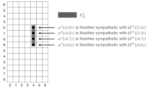
Figure 5: Values taken by the exact functor $\omega^{6}$ on singletons.

Theorem 79.

Each term $E^{r}_{pq}$ of the Leray-Serre spectral sequence admits a unique filtration

$$0=\mathrm{L}_{p+r-1}\leq\cdots\leq\mathrm{L}_{p-r+(N+1)}=E_{pq}^{r}$$

such that

$$\mathrm{L}_{x}/\mathrm{L}_{x-1}\begin{cases}\text{is Noether sympathetic with ${\Omega}^{m}\{[x,y)\}$}&y\leq N+1\\ \text{is Noether sympathetic with ${\Omega}^{m-1}\{[y-(N+1),x)\}$}&else\end{cases}$$

for each $x\in[p+r,p-r+(N+1)]$.

Proof.

Follows from (96) and Lemma 78. ∎

Now let

$$\tau^{m}({I}):=\mathrm{JH}({\Omega}^{m}\{{I}\})$$

be the Jordan-Hölder vector of (the object type of) ${\Omega}^{m}\{{I}\}$. In particular, $\tau^{m}({I})$ is a function $\mathsf{S}(\mathsf{E})\to\mathbf{Z}\cup\{\infty\}$. Elements of $(\mathbf{Z}\cup\{\infty\})^{\mathsf{S}(\mathsf{E})}$ can be added coordinatewise. We say $\tau^{m}({I})$ is coordinatewise-finite if every coordinate of $\tau^{m}({I})$ is an integer.

Theorem 80 (Leray-Serre enumeration theorem for saecular persistence).

If $\tau^{m}({I})$ is coordinatewise-finite, then

$$\mathrm{JH}(B^{r}_{pq}) =\sum_{\max({I})\leq p-r}\tau^{m}({I})$$ (97)

$$\mathrm{JH}(Z^{r}_{pq}) =\sum_{\min({I})\leq p}\tau^{m}({I})+\sum_{\min({J})\leq p-r,\;\max({J})\leq p}\tau^{m-1}({J})$$ (98)

$$\mathrm{JH}(E^{r}_{pq}) =\sum_{p<s\leq N}\tau^{m}[p,s]+\sum_{s\leq p-r}\tau^{m-1}[s,p]$$ (99)

for all $p$, $q$, and $r$. Here intervals appearing as subscripts are compared via the partial order on ${\mathbb{I}}(\mathbf{I})$.

Proof.

Apply Proposition 75 to $\omega^{m}$. Combine this result with Equations (94)-(96) and Lemma 78. ∎

There is a natural way to extend any chain diagram $f:\{0,\ldots,N\}\to\mathsf{E}$ to an $\{0,\ldots,N\}$-constructible functor $g:\mathbf{R}\to\mathsf{E}$ such that $h_{a}=0$ for $a<0$ and $h_{a}=g_{\lfloor a\rfloor}$ for $a\in[0,N+1]$. For each $f^{m}$, apply this construction to obtain a constructible functor $g^{m}$; denote the corresponding type-$\mathsf{B}$ generalized persistence diagram by $\mathrm{PD}^{\mathsf{B}}_{m}$.

Theorem 81 (Leray-Serre enumeration theorem for generalized persistence).

Suppose that $\mathsf{E}$ is abelian and each vector $\tau_{m}({I})$ has finite support. Then Theorem 80 remains true if we replace $\tau_{m}[a,b)$ with $\mathrm{PD}^{\mathsf{B}}_{m}(a,b)$.

Proof.

Theorem 77 states that $\tau_{m}[a,b)=\mathrm{PD}^{\mathsf{B}}_{m}(a,b)$ for all $a,b\in\mathbf{R}$. ∎

Appendix A Free modular and distributive lattices

Theorem 82 (Birkhoff).

Let $\mathbf{L}$ be a bounded lattice and $\mathrm{P}=\hat{\mathbf{I}}\sqcup\mathbf{I}$ be the coproduct in $\mathsf{P}$ of two bounded totally ordered sets $\hat{\mathbf{I}}$ and $\mathbf{I}$. Suppose that $f:\mathrm{P}\to\mathbf{L}$ is an order-preserving function that preserves the bounds of both $\hat{\mathbf{I}}$ and $\mathbf{I}$. Let ${\mathbb{S}(\hat{\mathbf{I}}_{>0}\times\mathbf{I}_{>0})}$ be the sublattice of ${\mathbb{A}(\hat{\mathbf{I}}_{>0}\times\mathbf{I}_{>0})}$ consisting of all finite unions of sets of form $(0,{\hat{a}}]\times(0,a]$ for some ${\hat{a}}\in\hat{\mathbf{I}}$ and $a\in\mathbf{I}$. Finally, define $\hat{\lambda}({\hat{a}})=[0,{\hat{a}}]\times\mathbf{I}$ and $\lambda(a)=\hat{\mathbf{I}}\times[0,a]$. Then the following are equivalent.

1. There exists a modular sublattice of $\mathbf{L}$ containing the image of $f$.

2. There exists lattice homomorphism $h$ (which happens to preserve bounds) such that $f=h\mu$.

(100)

Proof.

The finite case is proved in [4, p. 66, III, Theorem 9]; the infinite case is left as an exercise. A complete treatment of the infinite case can be found in [24, Theorem 1.3.7]. ∎

Lemma 83.

Lattice $\mathbb{D}\mathbb{A}(\hat{\mathbf{I}}\sqcup\mathbf{I})$ is isomorphic to the free bounded distributive lattice on $\mathbb{A}^{2}(\hat{\mathbf{I}})\sqcup\mathbb{A}^{2}(\mathbf{I})$. Specifically, there exists a commutative diagram

(101)

where the lefthand diagonal arrow is defined as in Theorem , the righthand diagonal arrow is defined as in (38), and $\rho:(0,\hat{S}]\times(0,S]\mapsto\hat{\lambda}(\hat{S})\wedge\lambda(S)$.

Proof.

The proof is a straightforward exercise in definition checking. ∎

Appendix B CD extension of well-ordered bifiltrations in a complete, modular, upper continuous lattice

Here we prove Theorem 92.

Given a poset $\mathrm{P}$, let ${\mathbb{V}}({\mathrm{P}})$ denote the lattice of all finite (including empty) antichains in $\mathrm{P}$, ordered such that $S\leq T\iff S\subseteq\;{\downarrow}\;T$. Let ${\mathbb{S}(\mathrm{P})}$ denote the sublattice of ${\mathbb{A}(\mathrm{P})}$ composed of all finite (including empty) unions of sets of form $\;{\downarrow}\;p$.

Lemma 84.

For any poset $\mathrm{P}$ there exist mutually inverse isomorphisms

$$\phi:{\mathbb{S}(\mathrm{P})} \to{\mathbb{V}}({\mathrm{P}}),\quad S\mapsto\max(S)$$

$$\psi:{\mathbb{V}}({\mathrm{P}}) \to{\mathbb{S}(\mathrm{P})},\quad A\mapsto\;{\downarrow}\;A.$$

Proof.

Clearly $\phi\psi=1$ and $\psi\phi=1$. ∎

Lemma 85.

If $\mathbf{I}$ is a well ordered set then so is every linearization of $\mathbf{I}^{2}$.

Proof.

let $\sigma$ be a linearization of $\mathbf{I}^{2}$, and fix any nonempty subset $S\subseteq\sigma$. The subset $A=\min_{\mathbf{I}^{2}}(S)$ is an antichain in $\mathbf{I}^{2}$, so $i<i^{\prime}$ implies $j^{\prime}<j$ for any distinct elements $(i,j)$, $(i^{\prime},j^{\prime})\in A$. Since every nonempty subset $\{i:(i,j)\in A\}$ contains a minimum, it follows that every subset of $\{j:(i,j)\in A\}$ contains a maximum, and conversely. Thus $A$ is finite. Every element of $S$ has an $\mathbf{I}^{2}$-lower bound in $A$, hence also an $\sigma$-lower bound in $A$. Thus $S$ contains an $\sigma$-minimum element in $A$. ∎

Corollary 86.

If $\mathbf{I}$ is a well ordered set then so is every linearization of $\mathbb{A}(\mathbf{I})^{2}$.

Proof.

It is elementary to show that $\mathbf{I}$ is well ordered iff ${\mathbb{A}(\mathbf{I})}$ is well ordered. ∎

Lemma 87.

Let $\hat{\mathbf{I}}$ and $\mathbf{I}$ be totally ordered sets satisfying the ascending chain condition (ACC) or the descending chain condition (DCC), and set

$$\mathrm{P}:={\mathbb{A}^{2}(\hat{\mathbf{I}})}_{>0}\times{\mathbb{A}^{2}(\mathbf{I})}_{>0}$$ (102)

Then there exists an isomorphism

$$\phi:{\mathbb{V}}({\mathrm{P}})\to\mathbb{A}^{2}(\hat{\mathbf{I}}\sqcup\mathbf{I}) X\mapsto\bigcup_{(\hat{S},S)\in X}\{\hat{T}\sqcup T:\hat{T}\in\hat{S},\;T\in S\}.$$

Proof.

Let $U\in\mathbb{A}^{2}(\hat{\mathbf{I}}\sqcup\mathbf{I})$ be given. Then the maps

$$\hat{\xi}: \mathbb{A}^{2}(\hat{\mathbf{I}})\to\mathbb{A}^{2}(\mathbf{I}),\quad\hat{S}\mapsto\{T\in{\mathbb{A}(\mathbf{I})}:\hat{T}\sqcup T\in U\;\forall\;\hat{T}\in\hat{S}\}$$

$$\xi: \mathbb{A}^{2}(\mathbf{I})\to\mathbb{A}^{2}(\hat{\mathbf{I}}),\quad S\mapsto\{\hat{T}\in{\mathbb{A}(\hat{\mathbf{I}})}:\hat{T}\sqcup T\in U\;\forall\;T\in S\}$$

satisfy

$$\hat{\xi}(\hat{S})\leq S \iff \hat{T}\sqcup T\in U\;\;\forall\;(\hat{T},T)\in\hat{S}\times S \iff \xi(S)\leq\hat{S}.$$

In particular, $\hat{\xi}$ and $\xi$ are polarities. Consequently, these maps restrict to mutually inverse poset anti-isomorphisms between the images of the closure operators ${\mathrm{cl}}:=\hat{\xi}\xi$ and $\hat{{\mathrm{cl}}}:=\xi\hat{\xi}$. If

$$A :=\{(\hat{S},\hat{\xi}(\hat{S})):\hat{S}\in\mathrm{Im}({\mathrm{cl}}^{*})\}=\{(\xi(S),S):S\in\mathrm{Im}({\mathrm{cl}})\}$$

and

$$\psi(U) :=\{(\hat{S},S)\in A:\hat{S}\neq\emptyset,\;S\neq\emptyset\}$$

then by construction

$$U=\phi(\psi(U))$$

Moreover, since $\mathrm{P}$ is the product of two totally ordered sets satisfying ACC (respectively, DCC), and since $A$ is an antichain in $\mathrm{P}$, only finitely many elements can lie in $A$. Thus

$$\psi(U)\in{\mathbb{V}}({\mathrm{P}}).$$

Consequently $\psi$ yields a well-defined map ${\mathbb{V}}({\mathrm{P}})\to\mathbb{A}^{2}(\hat{\mathbf{I}}\sqcup\mathbf{I})$. We have already seen that $\phi\psi=1$. It is straightforward to check that $\psi\phi=1$, also. ∎

Corollary 88.

If $\hat{\mathbf{I}}$ and $\mathbf{I}$ are totally ordered sets satisfying ACC, then

$$\mathbb{A}^{2}(\hat{\mathbf{I}}\sqcup\mathbf{I})={\mathbb{S}}^{2}(\hat{\mathbf{I}}\sqcup\mathbf{I}).$$

Proof.

Let $\phi$ be defined as in Lemma 87. Since ${\mathbb{A}^{2}(\hat{\mathbf{I}})}_{>0}$ and ${\mathbb{A}^{2}(\mathbf{I})}_{>0}$ satisfy ACC, to each ordered pair $(\hat{S},S)$ in the product (102) corresponds a pair of down-closed sets s $\hat{T}=\max S$ and $T=\max S$ such that

$$\phi(\{\hat{S},S\})=\;{\downarrow}\;(\hat{T}\sqcup T).$$

It follows from surjectivity of $\phi$ that every element of $\mathbb{A}^{2}(\hat{\mathbf{I}}\sqcup\mathbf{I})$ can be expressed as a finite union of sets of form $\;{\downarrow}\;(\hat{T}\sqcup T)$. ∎

Corollary 89.

If $\mathbf{I}$ and $\hat{\mathbf{I}}$ satisfy ACC then $\mathbb{A}^{2}(\hat{\mathbf{I}}\sqcup\mathbf{I})$ is algebraic.

Proof.

Let $U\in\mathbb{A}^{2}(\hat{\mathbf{I}}\sqcup\mathbf{I})$ be given. One has $U=\;{\downarrow}\;\max(U)$ by Corollary 88, so

$$\textstyle U\leq\bigvee S\iff\max(U)\subseteq\bigcup S.$$

for any $S\subseteq\mathbb{A}^{2}(\hat{\mathbf{I}}\sqcup\mathbf{I})$. Since $\max(U)$ is finite, it follows that $U$ is compact. ∎

Lemma 90.

Every lattice homomorphism $f$ from an algebraic lattice $\mathbf{M}$ to an arbitrary lattice $\mathbf{L}$ preserves infinite joins.

Proof.

Let $S$ be a nonempty subset of $\mathbf{M}$. By hypothesis there exists a finite subset $T\subseteq S$ such that $\bigvee S=\bigvee T$. One has

$$\textstyle f(\bigvee S)=f(\bigvee T)=\bigvee f(T)\leq\bigvee f(S)$$

The reverse inequality holds by definition of least upper bound, so strict equality holds throughout. ∎

Theorem 91 (Grandis).

Let $\hat{\mathrm{K}}:\hat{\mathbf{I}}\to\mathbf{L}$ and $\mathrm{K}:\mathbf{I}\to\mathbf{L}$ be order-preserving maps from totally ordered sets to a modular lattice $\mathbf{L}$. Then there exists a unique lattice homomorphism

$$\Lambda:{\mathbb{S}({\hat{\mathbf{I}}}_{>0}\times{\mathbf{I}}_{>0})}\to\mathbf{L}$$

such that

$$\Lambda(\;{\downarrow}\;(\hat{a},a))=\hat{\mathrm{K}}(\hat{a})\wedge\mathrm{K}(a)$$ (103)

for each $(\hat{a},a)\in{\hat{\mathbf{I}}}_{>0}\times\mathbf{I}$.

Remark 20.

To each poset $\mathrm{R}$ corresponds an anti-isomorphism

$$\phi:{\mathbb{A}(\mathrm{R})}\to{\mathbb{A}(\mathrm{R}^{*})}, S\mapsto\mathrm{R}-S.$$

Through repeated application, this construction can produce an anti-isomorphism $\phi^{(m)}:\mathbb{A}^{m}(\mathrm{P})\to\mathbb{A}^{m}(\mathrm{P}^{*})$ for any positive $m$.

Theorem 92.

Let $\hat{\mathbf{I}}$ and $\mathbf{I}$ be well-ordered sublattices of a complete upper continuous lattice $\mathbf{L}$. Let $\hat{\mathbf{J}}$ and $\mathbf{J}$ denote the smallest $\forall$-complete sublattices containing $\hat{\mathbf{I}}$ and $\mathbf{I}$, respectively. If there exists a modular sublattice $\mathbf{Q}\subseteq\mathbf{L}$ such that $\hat{\mathbf{J}}\cup\mathbf{J}\subseteq\mathbf{Q}$, then there exists a $\forall$-complete CD sublattice $\mathbf{Q}^{\prime}\subseteq\mathbf{L}$ such that $\hat{\mathbf{J}}\sqcup\mathbf{J}\subseteq\mathbf{Q}^{\prime}$.

Proof.

Let $\hat{\mathrm{K}}:\hat{\mathbf{I}}\to\mathbf{L}$ and $\mathrm{K}:\mathbf{I}\to\mathbf{L}$ be the inclusions of two well-ordered sets. Since $\mathbf{L}$ is complete, each of these maps factors through a complete totally ordered (hence completely distributive) sublattice. Thus $\hat{\mathrm{K}}$ and $\mathrm{K}_{f}$ have CDF extensions

$$\hat{\mathrm{K}}:\mathbb{A}^{2}(\hat{\mathbf{I}})\to\mathbf{L} \mathrm{K}:\mathbb{A}^{2}(\mathbf{I})\to\mathbf{L}.$$

By Theorem 91, this pair of maps extends to a lattice homomorphism

$$\Lambda:{\mathbb{S}({\mathbb{A}^{2}(\hat{\mathbf{I}})}_{>0}\times{\mathbb{A}^{2}(\mathbf{I})}_{>0})}\to\mathbf{L}$$

satisfying (103). Lemmas 84 and 87 yield an isomorphism

$$\theta:{\mathbb{S}({\mathbb{A}^{2}(\hat{\mathbf{I}})}_{>0}\times{\mathbb{A}^{2}(\mathbf{I})}_{>0})}\xrightarrow{\cong}\mathbb{A}^{2}(\hat{\mathbf{I}}\sqcup\mathbf{I})$$

where

$$\theta(\;{\downarrow}\;(\hat{S},S)):=\{\hat{T}\sqcup T:\hat{T}\in\hat{S},\;T\in S\}.$$ (104)

Every element of the complete lattice $\mathbb{A}^{2}(\hat{\mathbf{I}}\sqcup\mathbf{I})$ can be expressed as a finite join of elements of form (104). By abuse of notation, we will identify $\Lambda$ with $\Lambda\theta^{-1}$.

We claim that

$$\Lambda(\;{\downarrow}\;(\hat{S},S))=\bigvee_{\hat{T}\in\hat{S},\;T\in S}\Lambda(\;{\downarrow}\;(\;{\downarrow}\;\hat{T},\;{\downarrow}\;T))=\bigvee_{\hat{T}\in\hat{S},\;T\in S}\hat{\mathrm{K}}(\;{\downarrow}\;\hat{T})\wedge\mathrm{K}(\;{\downarrow}\;T)$$

for each $\hat{S}\in{\mathbb{A}^{2}(\hat{\mathbf{I}})}_{>0}$ and each $S\in{\mathbb{A}^{2}(\mathbf{I})}_{>0}$. This identity can be checked in three cases. In the first case, suppose that $\hat{S}$ and $S$ each contain a maximum element. Then the desired conclusion is vacuous. In the second case suppose that at least one of $\hat{S}$ and $S$ contains a maximum element. Here the desired conclusion holds by upper continuity. In the third case, allow that neither $\hat{S}$ nor $S$ may contain a maximum. Then a second application of upper continuity, applied to the already-established second case, yields desired conclusion, and the identity holds in full generality.

Now fix an arbitrary subset $W\subseteq\mathbb{A}^{2}(\hat{\mathbf{I}}\sqcup\mathbf{I})$, and choose a finite sequence of pairs $(\hat{S}_{m},S_{m})$ such that $\bigvee W=\bigcup_{m}\theta(\;{\downarrow}\;(\hat{S},S))$. One then has

$$\Lambda({\textstyle\bigvee W})=\bigvee_{m}\Lambda\;{\downarrow}\;(\hat{S}_{m},S_{m})=\bigvee_{m}\bigvee_{(\hat{T},T)\in\hat{S}_{m}\times S_{m}}\Lambda(\;{\downarrow}\;(\;{\downarrow}\;\hat{T},\;{\downarrow}\;T))\leq\bigvee\Lambda(W).$$

The reverse inequality holds by the definition of join, so $\Lambda(\bigvee W)=\bigvee\Lambda(W)$. As $W$ was arbitrary, it follows that $\Lambda$ preserves arbitrary joins.

Since $\mathbb{A}^{2}(\hat{\mathbf{I}}\sqcup\mathbf{I})$ is anti-isomorphic to $\mathbb{A}^{2}(\hat{\mathbf{I}}^{*}\sqcup\mathbf{I}^{*})$ by Remark 20, and the latter is algebraic by Corollary 89, it follows from Lemma 90 that $\Lambda$ preserves arbitrary nonempty meets. It preserves the empty meet by construction. Therefore $\Lambda$ is complete. The image of $\Lambda$ is thus a complete, completely distributive sublattice of $\mathbf{L}$ containing $\hat{\mathbf{I}}$ and $\mathbf{I}$. The desired conclusion follows. ∎

Appendix C Proof of Theorems 1 - 8

Proof of Theorem 1 .

The lattice of subobjects in any category of $R$ modules is complete and upper-continuous. Therefore existence of the CD homomorphism follows from the well-ordered criterion in Theorem 40. ∎

Proof of Theorem 2 .

Existence and uniqueness follow from Theorems 1 and 18. ∎

Proof of Remark 1 .

When $\mathbf{I}$ is finite, each saecular filtration takes finitely many values. The saecular BD homomorphism exists, and coincides with the saecular CD homomrophism. If each $f_{a}$ has finite height, then the saecular CD homomorphism exists for similar reasons. Note, in particular, that we do not require $\mathrm{Sub}(f_{a})$ to be a complete lattice, for any $a$. ∎

Proof of Theorem 3 .

To establish existence of the saecular CD homomorphism, first note that $f$ admits a saecular BDH, by Theorem 46. The image of this homomorphism is a distributive (a fortiori, modular) sublattice of $\mathrm{Sub}_{f}$ which contains the images of the FCD homomorphisms $\hat{\mathrm{K}}_{f}(\hat{\mathbf{I}}):\mathbb{A}^{2}(\hat{\mathbf{I}})\to\mathrm{Sub}_{f}$ and $\mathrm{K}_{f}(\mathbf{I}):\mathbb{A}^{2}(\mathbf{I})\to\mathrm{Sub}_{f}$. Therefore the saecular filtrations factor through a $\forall$-complete CD sublattice of $\mathrm{Sub}(f)$, by Theorem 92. Thus the SCDH exists.

The SCDH is natural, by 47. The saecular coset factors and cokernel factors of $f$ are therefore interval functors, by Theorem 63. ∎

Proof of Theorem 4.

Follows from Theorem 34. ∎

Proof of Theorem 5.

This is identical to Theorem 77. ∎

Proof of Theorem 6.

Follows from Theorems 35 and 61. ∎

Proof of Theorem 7.

If $\mathsf{E}$ is p-exact, then this result follows from exactness of the SCDI functor. If $\mathsf{E}=\mathsf{Group}$, then the desired conclusion follows from property (73) of the quasi-regular functor; in particular, this property implies isomorphism between $\frac{|\;{\downarrow}\;_{{\mathbb{I}}(\mathbf{I})}{I}|}{|\;{\mathring{\downarrow}}\;_{{\mathbb{I}}(\mathbf{I})}{I}|}$ and $\frac{|\;{\downarrow}\;_{\sigma}{I}|}{|\;{\mathring{\downarrow}}\;_{\sigma}{I}|}$. ∎

Proof of Theorem 8 and Remark 4.

If $\mathrm{P}$ is a poset, then each down-set $S\in{\mathbb{A}(\mathrm{P})}$ is a join (i.e. union) of sets of form $S=\bigvee_{p\in S}\;{\downarrow}\;_{\mathrm{P}}(p)$ As a special case, when $\mathrm{P}={\mathbb{A}(\hat{\mathbf{I}}\sqcup\mathbf{I})}$ or $\mathrm{P}={\mathbb{J}}(\hat{\mathbf{I}}\sqcup\mathbf{I})$, each element of $\mathbb{A}(\mathrm{P})$ can be expressed as a join of sets of form $S=\bigvee_{\hat{T}\sqcup T\in S}\;{\downarrow}\;_{\mathrm{P}}(\hat{T}\sqcup T)$. Since ${\Omega}_{\mathbb{J}}:=\mathsf{SCDI}(f)$ and ${\Omega}:=\mathsf{SCD}(f)$ are $\forall$-complete lattice homomorphisms, it follows that

$$\textstyle{\Omega}_{\mathbb{J}}S={\Omega}_{\mathbb{J}}\bigvee_{\hat{T}\sqcup T\in S}\;{\downarrow}\;_{\mathrm{P}}(\hat{T}\sqcup T)=\bigvee_{\hat{T}\sqcup T\in S}{\Omega}_{\mathbb{J}}\;{\downarrow}\;_{\mathrm{P}}(\hat{T}\sqcup T)=\bigvee_{\hat{T}\sqcup T\in S}{\Omega}\;{\downarrow}\;_{\mathrm{P}}(\hat{T}\sqcup T)$$

Since we identify ${\mathbb{I}}(\mathbf{I})$ with ${\mathbb{J}}(\hat{\mathbf{I}}\sqcup\mathbf{I})$, the desired conclusion follows from the observation that for any ${I}=\hat{T}-\pi(T)$,

$${\Omega}\;{\downarrow}\;_{\mathrm{P}}(\hat{T}\sqcup T)=\hat{\mathrm{K}}_{f}(\;{\downarrow}\;\hat{T})\wedge\mathrm{K}_{f}(\;{\downarrow}\;T)=\textstyle(\bigwedge_{{\hat{a}}\notin\hat{T}}\hat{\mathrm{K}}_{f}({\hat{a}}))\wedge(\bigwedge_{a\notin T}\mathrm{K}_{f}(a))=A_{\pi(\hat{T}),T}$$

∎

References

- [1] Basu, S., and Parida, L. Spectral sequences, exact couples and persistent homology of filtrations. Expositiones Mathematicae 35, 1 (2017), 119–132.
- [2] Batan, M. A., Pamuk, M., and Varli, H. Persistent homotopy. arXiv preprint arXiv:1909.08865 (2019).
- [3] Bauer, U., and Lesnick, M. Persistence diagrams as diagrams: A categorification of the stability theorem. In Topological Data Analysis. Springer, 2020, pp. 67–96.
- [4] Birkhoff, G. Lattice Theory, 3 ed., vol. 25 of American Mathematical Society Colloquium Publications. American Mathematical Society, Providence, RI, 1967.
- [5] Blumberg, A., and Lesnick, M. Universality of the homotopy interleaving distance. arXiv preprint arXiv:1705.01690 (2017).
- [6] Botnan, M., and Crawley-Boevey, W. Decomposition of persistence modules. Proceedings of the American Mathematical Society 148, 11 (2020), 4581–4596.
- [7] Browning, T., and Vishe, P. Rational curves on smooth hypersurfaces of low degree. Algebra & Number Theory 11, 7 (2017), 1657–1675.
- [8] Burghelea, D., and Dey, T. K. Topological persistence for circle-valued maps. Discrete & Computational Geometry 50, 1 (2013), 69–98.
- [9] Burghelea, D., and Haller, S. Topology of angle valued maps, bar codes and Jordan blocks. Journal of Applied and Computational Topology 1, 1 (2017), 121–197.
- [10] Carlsson, G., and de Silva, V. Zigzag persistence. Found. Comput. Math. 10, 4 (2010), 367–405.
- [11] Carlsson, G., de Silva, V., and Morozov, D. Zigzag persistent homology and real-valued functions. In Proceedings 25th ACM Symposium on Computational Geometry (SoCG) (2009), pp. 247–256.
- [12] Carlsson, G., Ishkhanov, T., de Silva, V., and Zomorodian, A. On the local behavior of spaces of natural images. International Journal of Computer Vision 76, 1 (Jan. 2008), 1–12.
- [13] Carlsson, G., Zomorodian, A., Collins, A., and Guibas, L. J. Persistence barcodes for shapes. International Journal of Shape Modeling 11, 02 (2005), 149–187.
- [14] Collins, A., Zomorodian, A., Carlsson, G., and Guibas, L. A barcode shape descriptor for curve point cloud data. In Eurographics Symposium on Point-Based Graphics (ETH, Zürich, Switzerland, 2004), M. Alexa and S. Rusinkiewicz, Eds.
- [15] Costa, J. P., Johansson, M. V., and Škraba, P. Variable sets over an algebra of lifetimes: a contribution of lattice theory to the study of computational topology. arXiv preprint arXiv:1409.8613 (2014).
- [16] Costa, J. P., Škraba, P., and Vejdemo-Johansson, M. Aspects of an internal logic for persistence. In Proceedings of the Applied Topology Conference 2013, Journal of Topological Methods in Nonlinear Analysis (2013).
- [17] Edelsbrunner, H., and Harer, J. Computational Topology: an Introduction. American Mathematical Society, Providence, RI, 2010.
- [18] Edelsbrunner, H., Letscher, D., and Zomorodian, A. Topological persistence and simplification. In Proceedings 41st Annual Symposium on Foundations of Computer Science (2000), pp. 454–463.
- [19] Edelsbrunner, H., Letscher, D., and Zomorodian, A. Topological persistence and simplification. Discrete and Computational Geometry 28 (2002), 511–533.
- [20] Edelsbrunner, H., and Zomorodian, A. Computing linking numbers of a filtration. In Algorithms in Bioinformatics, O. Gascuel and B. Moret, Eds., vol. 2149 of Lecture Notes in Computer Science. Springer Berlin / Heidelberg, 2001, pp. 112–127.
- [21] Frosini, P. Measuring shapes by size functions. In Intelligent Robots and Computer Vision X: Algorithms and Techniques (1992), D. P. Casasent, Ed., vol. 1607, International Society for Optics and Photonics, SPIE, pp. 122 – 133.
- [22] Frosini, P., and Mulazzani, M. Size homotopy groups for computation of natural size distances. Bulletin of the Belgian Mathematical Society - Simon Stevin 6, 3 (1999), 455 – 464.
- [23] Gabriel, P. Unzerlegbare darstellungen i. Manuscripta Mathematica 6, 1 (1972), 71–103.
- [24] Grandis, M. Homological Algebra, The Interplay of Homology with Distributive Lattices and Orthodox Semigroups. World Scientific, 2012.
- [25] Henselman, G., and Ghrist, R. Matroid filtrations and computational persistent homology. arXiv preprint arXiv:1606.00199 (2016).
- [26] Henselman-Petrusek, G. Matroids and canonical forms: theory and applications. PhD thesis, University of Pennsylvania, May 2017.
- [27] Henselman-Petrusek, G. Semitopological coproducts and free objects on totally ordered sets in some categories of complete, distributive, modular, and algebraic lattices. Available at https://gregoryhenselman.org (2019).
- [28] Jardine, J. F. Persistent homotopy theory. arXiv preprint arXiv:2002.10013 (2020).
- [29] Letscher, D. On persistent homotopy, knotted complexes and the alexander module. In Proceedings of the 3rd Innovations in Theoretical computer Science Conference (2012), pp. 428–441.
- [30] McCleary, A., and Patel, A. Edit distance and persistence diagrams over lattices. arXiv preprint arXiv:2010.07337 (2020).
- [31] Mémoli, F., and Zhou, L. Persistent homotopy groups of metric spaces. arXiv preprint arXiv:1912.12399 (2019).
- [32] Méndez, D., and Sánchez-García, R. J. A directed persistent homology theory for dissimilarity functions, 2021.
- [33] Morozov, D., de Silva, V., and Vejdemo-Johansson, M. Persistent cohomology and circular coordinates. Discrete and Computational Geometry 45, 4 (2011), 737—759.
- [34] Patel, A. Generalized persistence diagrams. Journal of Applied and Computational Topology 1, 3 (2018), 397–419.
- [35] Polterovich, L., and Shelukhin, E. Autonomous Hamiltonian flows, Hofer’s geometry and persistence modules. Selecta Mathematica 22, 1 (2016), 227–296.
- [36] Polterovich, L., Shelukhin, E., and Stojisavljević, V. Persistence modules with operators in morse and floer theory. arXiv preprint arXiv:1703.01392 (2017).
- [37] Robins, V. Towards computing homology from finite approximations. In Proceedings of the 14th Summer Conference on General Topology and its Applications (Brookville, NY, 1999) (1999), vol. 24, pp. 503–532.
- [38] Robins, V. Computational topology for point data: Betti numbers of -shapes. In Morphology of Condensed Matter, K. Mecke and D. Stoyan, Eds., vol. 600 of Lecture Notes in Physics. Springer Berlin / Heidelberg, 2002, pp. 261–274.
- [39] Romero, A. A computational review of spectral sequences and applications. Zaragoza (2018).
- [40] Romero, A., Heras, J., Rubio, J., and Sergeraert, F. Defining and computing persistent z-homology in the general case. arXiv preprint arXiv:1403.7086 (2014).
- [41] Tunnicliffe, W. The free completely distributive lattice over a poset. Algebra Universalis 21, 1 (1985), 133–135.
- [42] Usher, M., and Zhang, J. Persistent homology and floer–novikov theory. Geometry & Topology 20, 6 (2016), 3333–3430.
- [43] Zomorodian, A., and Carlsson, G. Computing persistent homology. Discrete Comput. Geom. 33, 2 (2005), 249–274.