VLT/MUSE and ATCA observations of the host galaxy of the
short GRB 080905A at $z$=0.122

Abstract

Short-GRB progenitors could come in various flavors, depending on the nature of the merging compact stellar objects (including a stellar-mass black hole or not) or depending on their ages (millions or billions of years). At a redshift of $z$=0.122, the nearly face-on spiral host of the short GRB 080905A is one of the closest short-GRB host galaxies identified so far. This made it a preferred target to explore spatially resolved star-formation and to investigate the afterglow position in the context of its star formation structures. We used VLT/MUSE integral-field unit observations, supplemented by ATCA 5.5/9.0 GHz radio-continuum measurements and publicly available HST data, to study the star-formation activity in the GRB 080905A host galaxy. The MUSE observations reveal that the entire host is characterized by strong line emission. Using the H$\alpha$ line flux, we measure for the entire galaxy an SFR of about 1.6 $M_{\odot}$ yr^-1, consistent with its non-detection by ATCA. Several individual star-forming regions are scattered across the host. The most luminous region has a H$\alpha$ luminosity that is nearly four times as high as the luminosity of the Tarantula nebula in the Large Magellanic Cloud. Even though star-forming activity can be traced as close to about 3 kpc (in projection) distance to the GRB explosion site, stellar population synthesis calculations show that none of the H$\alpha$-bright star-forming regions is a likely birthplace of the short-GRB progenitor.

1 Introduction

To better understand the diversity in gamma-ray bursts (GRBs), host-galaxy studies offer a powerful observational tool. Early work in this respect goes back to times when GRB afterglows were not yet known. Before 1997, observations focused on a search for ’unusual’ or statistically rare galaxies in the smallest available GRB error boxes (Interplanetary Network error boxes; e.g., Atteia et al. 1987; Hurley et al. 1993; Hurley & Cline 1994) in order to find clues to the distance scale and underlying nature of the bursts (e.g., Boer et al. 1991; Vrba et al. 1995; Klose et al. 1996; Larson et al. 1996; Hurley et al. 1997; Larson & McLean 1997; Schaefer et al. 1998). Although these observations did not identify valid host candidates, they did support the notion that bursts of extragalactic origins would be associated with normal host galaxies, i.e., not galaxies characterized by unusual physical parameters.

Once the first optical afterglow of a long GRB was discovered (Groot et al. 1997; van Paradijs et al. 1997), studies of GRB host galaxies quickly developed into a powerful approach to reveal additional information about the nature of GRB progenitors (e.g., Bloom et al. 1998; Djorgovski et al. 1998; Sokolov et al. 1999; Fruchter et al. 2006; Thöne et al. 2014; Lyman et al. 2017).

A milestone in the exploration of GRB host galaxies was the first identified long-GRB progenitor, GRB 980425/SN 1998bw (Galama et al. 1998). Due to its very low redshift ($z$=0.0085; Tinney et al. 1998), the host became the focus of several comprehensive observing campaigns, which provided substantial insight into the GRB explosion site and hence the nature of the GRB progenitor (e.g., Hammer et al. 2006; Christensen et al. 2008; Michałowski et al. 2009; Le Floc’h et al. 2012; Michałowski et al. 2014, 2015, 2016; Arabsalmani et al. 2015; Krühler et al. 2017).

Long before the first afterglow of a short GRB was discovered and localized at an arcsecond scale (GRB 050509B; Gehrels et al. 2005), convincing arguments were already in place that short GRBs could be linked to merging compact stellar binaries (for a review, see Nakar 2007), which naturally includes elliptical galaxies as their potential hosts. The discovery that the host of GRB 050509B was a giant elliptical ($z$=0.225; Gehrels et al. 2005; Hjorth et al. 2005; Bloom et al. 2006) confirmed this notion. Finally, the study of the hosts of short bursts received a substantial boost by the discovery of a physical link between the gravitational wave event GW170817 and the short GRB 170817A and the identification of its early-type host galaxy (e.g., Abbott et al., 2017; Coulter et al., 2017; Hjorth et al., 2017; Kasen et al., 2017; Smartt et al., 2017; Kim et al., 2017).

Several years ago our group started a comprehensive observing campaign designed to study the host-galaxy population of short GRBs in order to characterize their star formation activity, with particular emphasis on deep radio-continuum observations (GRB 071227: Nicuesa Guelbenzu et al. 2014; GRB 100628: Nicuesa Guelbenzu et al. 2015; GRB 050709: Nicuesa Guelbenzu et al. 2021). In Klose et al. (2019), we provided a first summary of this radio survey program and reported on 16 targeted short-GRB hosts.

So far, in two cases we have been able to supplement our ATCA and VLA radio observations by using the Multi-Unit Spectroscopic Explorer (MUSE; Bacon et al. 2010) mounted at the Very Large Telescope (VLT). First results were reported in Nicuesa Guelbenzu et al. (2021), where we studied in detail the host of GRB 050709. Here, we continue these studies and focus on the host of the short GRB 080905A. At a redshift of $z=0.1218\pm 0.0003$ (Rowlinson et al., 2010), the host of GRB 080905A is among the nearest short-GRB hosts detected to date (Berger 2014), qualifying it as one of the presently best targets for spatially resolved studies.

The structure of this work closely follows our previous study of GRB 050709, though our conclusions about the nature of these two hosts are very different. Throughout this paper, we adopt a flat universe with H₀ = 68 km s^-1 Mpc^-1, $\Omega_{\rm M}$=0.31, and $\Omega_{\Lambda}$=0.69 (Planck Collaboration et al. 2016). Then, for $z$=0.1218, the luminosity distance is $d_{L}=1.81\,\times\,10^{27}$ cm (585 Mpc), the age of the universe is 12.13 Gyr, and 1 arcsec corresponds to 2.25 kpc projected distance.

2 The Burst, Its Afterglow, and Its Host Galaxy

2.1 The Burst and Its Afterglow

The Neil Gehrels Swift Observatory (Gehrels et al. 2004) BAT telescope (Barthelmy et al. 2005) and Fermi/GBM (Meegan et al. 2009) triggered on GRB 080905A on 5 September 2008 at 11:58:54 UT (Bissaldi et al. 2008; Pagani et al. 2008). The BAT light curve showed three peaks with a total duration of $T_{90}$ (15–350 keV)=$1.0\pm 0.1$ s (Cummings et al. 2008). The lag time of the burst between the BAT [5–50 keV] and the [50–100 keV] channel was $4\pm 17$ ms, consistent with zero (Rowlinson et al. 2010), which is characteristic for the short-burst population (e.g., Gehrels et al. 2006; Norris & Bonnell 2006; Shao et al. 2017; Lu et al. 2018).

A fading X-ray afterglow was found by Swift/XRT (for the instrument description see Burrows et al. 2005) at coordinates R.A., decl. (J2000) =19:10:41.74, $-$18:52:48.8, with an error circle of 1$\farcs$6 (radius, 90% confidence; Evans et al. 2008), but no optical afterglow was detected with Swift/UVOT (Pagani et al. 2008; for UVOT: Roming et al. 2005). Even though the burst occurred in a crowded stellar field, a faint optical afterglow candidate ($R\sim$24 mag) was finally discovered 8 hr after the GRB trigger with the Nordic Optical Telescope (NOT) and with VLT/FORS2 at coordinates R.A., decl. (J2000) = 19:10:41.73, $-$18:52:47.3 ($\pm$0$\farcs$6; Malesani et al. 2008). Its fading was confirmed by follow-up observations with FORS2 1.5 days after the burst, and a host-galaxy candidate was identified (de Ugarte Postigo et al. 2008).

GROND, mounted at the MPG 2.2m telescope on ESO/La Silla (Greiner et al. 2008), started observing the field of GRB 080905A about 17.5 hr after the burst. Due to visibility constraints, observations could be performed for only 11 min. The combined $g^{\prime}r^{\prime}i^{\prime}z^{\prime}$-band image as well as the combined $JHK$-band image did not reveal the afterglow, even though the image depth reached $g^{\prime}r^{\prime}i^{\prime}z^{\prime}JHK$= 23.0, 22.8, 22.3, 21.9, 20.4, 19.9, and 19.6 (AB magnitudes; Nicuesa Guelbenzu et al. 2012). Published work later showed that at the time of the GROND observations, the magnitude of the afterglow was around $R_{C}=24$ (Rowlinson et al. 2010), about 1 mag below GROND’s detection limit for an 11 min exposure.

No emerging supernova component was detected following the burst, supporting a non-collapsar origin of this event (Rowlinson et al. 2010).

2.2 The GRB Host Galaxy

Using VLT data, the afterglow and its host were analyzed in detail by Rowlinson et al. (2010). The afterglow coordinates were refined by these authors to R.A., decl. (J2000) = 19:10:41.71, $-$18:52:47.62 ($\pm$0$\farcs$76). The afterglow was located in the outer arm of a barred spiral galaxy at $z=0.1218\pm 0.0003$. The projected offset of the burst from the light center of the galaxy was $\sim$18.5 kpc.

Rowlinson et al. (2010) derived an absolute host magnitude of $M_{V}=-21$ mag and a mass in old stars (based on VLT $K_{s}$-band data) of ($2\pm 1)\,\times\,10^{10}\,M_{\odot}$. Because the field is crowded with Galactic foreground stars, no star-formation rate (SFR) could be derived for this galaxy by these authors.

The field was also observed by HST on two different occasions, in October 2011 and April 2012 (program ID 12502; PI: A. Fruchter). Figure 1 shows the F606W image of the field (archival file name: ibsh16030_-drz.fits), where the barred spiral morphology of the galaxy appears clearly (Fong & Berger 2013). Its general shape strongly resembles NGC 1365 in the Fornax cluster (for an elegant mathematical characterization of the spiral pattern of this galaxy see Ringermacher & Mead 2009).

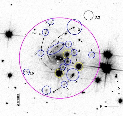
Figure 1: HST/F606W image (program ID 12502; PI: A. Fruchter) of the field of GRB 080905A taken on 2012-04-14. The afterglow (AG, error circle 0$\farcs$76 radius, in black; Rowlinson et al. 2010) was located $\sim$8$\farcs$5 from the center of its host. Three bright Galactic foreground stars are encircled by a yellow line. Shown in blue are several star-forming complexes that can be identified by their strong H$\alpha$ emission (Sect. 4). They are numbered according to their R.A. (Table 1); the three H$\alpha$-brightest regions are labeled with letters (A, B, D), however. Region C is the galaxy’s bar, region X is the star-forming region nearest (in projection) to the AG position (Sect. 4.4). The large circle in magenta encompasses the region for which we measure the total star formation rate (Sect. 4.4). Also shown is a reference star (about 2 arcsec east of #8) for which we measure on the HST image R.A., decl. (J2000) = 19:10:42.323, $-$18:52:49.88 $(\pm$0$\farcs$08). The spiral pattern of the galaxy is sketched by broken lines.

2.3 Is the Suspected Host a Foreground Galaxy?

For GRB 080905A no redshift measurement could be obtained via afterglow spectroscopy. This raises the question of the robustness of the suspected association between GRB 080905A and the $z$=0.122 spiral galaxy, an issue that has already been addressed by other authors. In brief, there is no ultimate proof that the burst was associated with this galaxy. However, there is no convincing counter argument either. There are at least two studies published in the literature that have to be mentioned in this respect.

(i) Deep HST/F160W imaging revealed a faint (AB$\sim$26 mag) galaxy close to the position of the optical AG (offset $\sim$0$\farcs$7; Fong & Berger 2013). Its small angular size ($<$1 arcsec) might be indicative of a redshift $z>$1. According to Fong & Berger (2013), the probability of a chance coincidence $p$ between the burst and this galaxy is 0.08, compared to $p$=0.01 for the $z=0.122$ galaxy. Even though this defines the faint galaxy as another host-galaxy candidate, the much smaller $p$ favors the assumption that the large spiral is the host.

(ii) D’Avanzo et al. (2014) performed a statistical analysis of all short GRBs and found that for a redshift of 0.122 the burst 080905A is an outlier among the short-GRB ensemble in the $E_{\rm peak}-E_{\rm iso}$ diagram. Given its observed $E_{\rm peak}$, the isotropic equivalent energy calculated by these authors ($3.2\pm 0.3\,\times\,10^{49}$ erg) lies more than a factor of 10 below the expectations. As pointed out by these authors, a higher redshift could solve this apparent conundrum. However, at that time, their statistics were based on a relatively small comparison sample (10 short bursts). More recent data, including many more short bursts, no longer support the conclusion that GRB 080905A is an outlier in the $E_{\rm peak}-E_{\rm iso}$ diagram (Zhang et al. 2018, their figure 3). Hence there is no longer any statistical argument at hand that points to a potentially much higher redshift of this burst.

We conclude that the currently best strategy is to follow Occam’s razor and to adopt the hypothesis (Rowlinson et al. 2010) that GRB 080905A was associated with the large barred spiral at $z$=0.122.

3 Observations and Data Reduction

3.1 ATCA Radio-continuum Observations

Radio-continuum observations of the host of GRB 080905A were performed in two runs several years after the burst on 2013 July 20 and on 2015 October 25 in the 5.5 and 9.0 GHz bands (corresponding to wavelengths of 6 and 3 cm, respectively) with the Australia Telescope Compact Array (ATCA). The total combined observing time was 10.5 hr (1st run: 1.51 hr, 2nd run: 9.04 hr). Both observing runs were executed using the upgraded Compact Array Broadband Backend (CABB) detector (Wilson et al. 2011) and all six 22 m antennae with the 6 km baseline (configuration 6A; program ID: C2840, PI: A. Nicuesa Guelbenzu). In both runs, phase calibration was performed by observing the quasar PKSB 1908–201 (redshift $z=1.119$) for 3 minutes every hour followed by 57 minute integrations on target. This quasar has a radio flux of $F_{\nu}$(5.5 GHz) = 2.79 Jy and $F_{\nu}$(9.0 GHz)=3.0 Jy.

Data reduction was performed using the Multichannel Image Reconstruction, Image Analysis and Display (MIRIAD) software package for ATCA radio interferometry (for details, see Sault et al. 1995). The Briggs ”robust” parameter (Briggs, 1995) was varied between 0.0 and 2.0. The resulting 1 $\sigma_{\rm rms}$ of the deconvolved images was between 5.4 and $5.7~{}\mu$Jy beam^-1 at 5.5 GHz and between 6.5 and $7.4~{}\mu$Jy beam^-1 at 9.0 GHz. We selected the results that gave the best compromise between sensitivity and resolution (robust = 0.5). The width of the synthesized beam (major axis, minor axis) then was 7$\farcs$9$\,\times\,$1$\farcs$4 at 5.5 GHz and 4$\farcs$8$\,\times\,$0$\farcs$9 at 9.0 GHz.

Despite the relatively small redshift, no radio source was detected superimposed on the GRB host galaxy (Fig. 2). The measured $3\sigma$ upper limits per beam are $F_{\nu}($5.5 GHz$)<17~{}\mu$Jy and $F_{\nu}($9.0 GHz$)<20~{}\mu$Jy.

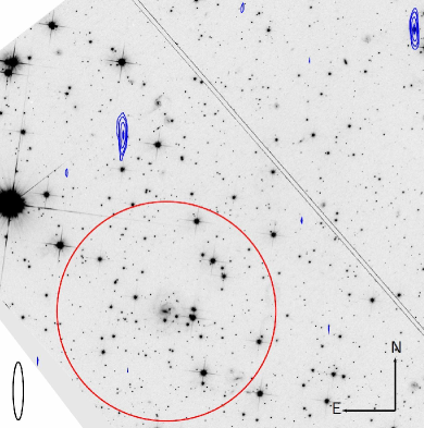
Figure 2: The field of GRB 080905A (field of view 2${}^{\prime}\times 2^{\prime}$) as seen by ATCA in the 5.5 GHz radio-continuum band, overplotted the HST/WCS3 F814W image taken on 2012 April 14 (program ID 12502; PI: A. Fruchter). Radio contour levels (in blue) refer to $F_{\nu}$=20, 30, 50, and 80 $\mu$Jy. To guide the eye, a circle with a radius of 30 arcsec centered at the suspected GRB host galaxy is drawn (red color). The radio source closest to the host ($F_{\nu}$(5.5 GHz) = 92$\pm$11 $\mu$Jy) is centered at the position of a tight pair of (interacting?) galaxies at (radio-) coordinates R.A., decl. (J2000) = 19:10:42.854, $-$18:52:06.39 ($\pm$0$\farcs$10, $\pm$0$\farcs$65, resp.). The radio source in the NW corner ($F_{\nu}$(5.5 GHz) = 91$\pm$8 $\mu$Jy) is an anonymous quasi-stellar object at (radio-) coordinates R.A., decl. (J2000) = 19:10:37.217, $-$18:51:37.62 ($\pm$0$\farcs$07, $\pm$0$\farcs$39, resp.). The beam size and orientation is shown in the lower left corner.

3.2 VLT/MUSE Observations

Observations with VLT/MUSE were performed on 30 May 2017 (program ID: 099.D-0115A, PI: T. Krühler). Eight dithered exposures of $\sim$700 s each were obtained. Observations were executed using the wide-field mode in which MUSE offers a field of view of $1^{\prime}\,\times\,1^{\prime}$. In this mode, MUSE provides a pixel (spaxel) resolution of 0$\farcs$2. The MUSE data cover the wavelength range from 480 to 930 nm with a resolving power of 1770 (480 nm) - 3590 (930 nm). During the observations, the seeing was between 0$\farcs$9 (at 9000 Å) and 1$\farcs$1 (at 5000 Å).

The data were reduced following the methodology of Krühler et al. (2017), using version 1.2.1 of the MUSE data reduction pipeline provided by ESO (Weilbacher et al. 2012, 2014). The data were corrected for Galactic foreground reddening ($E(B-V)$=0.12 mag; Schlafly & Finkbeiner 2011), assuming an average Milky Way extinction law (Pei 1992) and $R_{V}=3.08$. For the flux calibration, the spectrophotometric standard star LTT3218 was observed at the beginning of the night.

Analogous to Nicuesa Guelbenzu et al. (2021) and following Krühler et al. (2017), we separated the stellar and gas-phase components of the galaxy in order to obtain accurate line flux measurements. We used the Starlight software package (Cid Fernandes et al. 2005, 2009) to model the stellar continuum using a combination of single stellar population models (Bruzual & Charlot 2003) and then subtracted the fitted stellar continuum model to obtain the gas-phase-only data cube (Fig. 3). In the following, we used this gas-phase cube only, except when we calculated the equivalent widths. In the latter case we used the combined cube (star + gas).

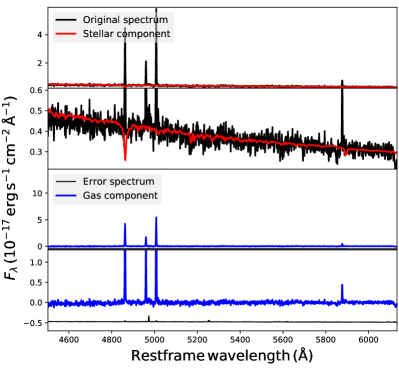
Figure 3: Spectrum and best-fit Starlight stellar continuum model corresponding to the 2x2 binned spectrum centered at the position of the HII region labeled A in Fig. 1, illustrating the separation of the stellar and gas-phase components. Top: original spectrum containing stellar and ionized gas emission (black) and our Starlight stellar continuum model fit (red). Top-middle: zoom-in of the continuum shown in the top panel. Bottom-middle: spectrum of the gas-phase-only component (blue) with the error spectrum indicated below in black. Bottom: zoom-in of the gas-phase-only component (blue) with the error spectrum now more visible (black).

3.3 Astrometry

In a first step, the HST image was aligned using saoimage DS9 version 8.1 (Joye & Mandel 2003) using The Fifth USNO CCD Astrograph Catalog, which provides positions with 10 to 70 mas precision (Zacharias et al. 2017). We double-checked the astrometric quality of the aligned image via a bright, anonymous, radio point source in our ATCA 5.5 GHz images at coordinates R.A., decl. (J2000) = 19:10:37.217, $-$18:51:37.615 ($\pm$0$\farcs$05; $F_{\nu}$(5.5 GHz) = 91$\pm$8 $\mu$Jy). For the relatively bright optical counterpart of this source (a spiral galaxy seen face-on) we measured on the HST image central coordinates R.A., decl. (J2000) = 19:10:37.221, $-$18:51:37.46 ($\pm$0$\farcs$05). Based on this procedure, we estimate the accuracy of our astrometry on the HST image to $\pm$0$\farcs$15. In a second step, we aligned the MUSE data cube with the HST image via stars visible in the HST image close to the target position. We estimate that our achieved relative astrometric accuracy between HST and MUSE is $\pm 0\farcs 2$ ($\pm$1 spaxel) in each direction.

4 Results

4.1 Emission-line Fluxes and Their Uncertainties

In order to measure the line fluxes, the numerical procedure (Krühler et al. 2017; Tanga et al. 2018) fits a Gaussian to an observed emission line. Errors in the calculated line flux per spaxel are a direct result of this fit. In addition, there are errors due to uncertainties in the continuum level at the position of an emission line (for a discussion of this issue, see also Erroz-Ferrer et al. 2019). In our spectra, this mainly affects the H$\beta$ line and becomes evident by an apparently unphysical low flux ratio H$\alpha$/H$\beta$ (Sect. 4.3).

In the following, when measuring a physical parameter for each emission line we always adopted a threshold for the signal-to-noise ratio (S/N). Consequently, if the flux in more than one emission line has to be used in order to calculate a certain physical quantity, the line with the smallest S/N determines if a certain spaxel enters the statistics or not. The results obtained in this way are shown in the following maps (see below).

In Appendix A we provide for all star-forming regions the measured luminosity in the five lines H$\alpha$, H$\beta$, [O iii] $\lambda$5007, [S ii] $\lambda$6718, and [N ii] $\lambda$6584. All spaxels with S/N$\geq$2 are used here. The number of spaxels that fulfills this criterion differs from line to line. Therefore, in general, these emission-line luminosities should not be used to calculate for a certain region an average $E(B-V)$, an average extinction-corrected SFR, or an average metallicity index (see also Sect. 4.3.3).

4.2 Radial Velocity Pattern and Dispersion Map

The radial velocity map shown in Fig. 4 is based on the H$\alpha$ emission line, where only spaxels with a signal-to-noise ratio S/N$\geq$5 are plotted. H$\alpha$-emitting gas can be traced up to about 7$\farcs$3 (16.5 kpc) away from the central bar of the galaxy.

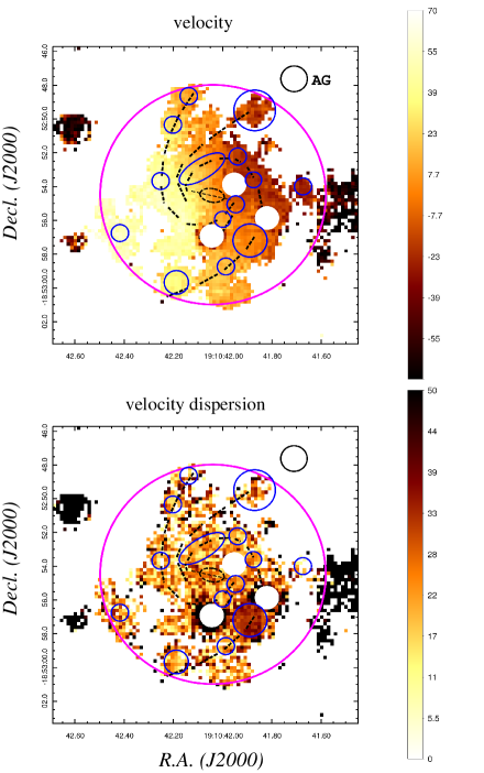
Figure 4: Radial velocity (top) and velocity dispersion map (bottom) of the H$\alpha$ emission line of the host of GRB 080905A. One spaxel ($0\farcs 2\,\times\,0\farcs 2$) corresponds to $0.45\,\times\,0.45$ kpc². Velocities are given in units of km s^-1; velocities are observed, not corrected for inclination. The circles have the same meaning as in Fig. 1. The signals from the three bright Galactic foreground stars inside the big circle (magenta) have been masked. Residuals from other bright Galactic foreground stars outside this circle have not been masked, however.

The main feature in Fig. 4 is a velocity gradient from NW to SE direction. The velocity map confirms that the galaxy is not seen exactly face-on. According to Rowlinson et al. (2010), the inclination angle is about 23 deg.

A comparison between the HST image (Fig. 1) and the H$\alpha$ velocity map reveals a spatial asymmetry in the H$\alpha$ emission component. MUSE detects a substantial amount of H$\alpha$-emitting gas in the eastern part of the galaxy around region #10, which has no counterpart on the western site of the galaxy. A possible explanation could be that this is interstellar gas stripped from the galaxy’s disk due to an interaction with a nearby galaxy. However, such a potential galaxy perturber cannot be identified in our data.

An additional clue about the H$\alpha$-emitting gas comes from the velocity dispersion map (Fig. 4, bottom). When calculating this map we adopted $10^{4}$ K warm gas ($\sigma_{\rm gas}$ = 9.1 km s^-1) and a MUSE line-spread function (LSF) of 2.5 Å at the wavelength of the redshifted H$\alpha$ line (see Fig. 15 in Bacon et al. 2017), which corresponds to an FWHM of 101 km s^-1 and a $\sigma_{\rm instr}$ of 43 km s^-1 (for more details on our procedure, see Nicuesa Guelbenzu et al. 2021). Neglecting the artificial features that result from the removal of the Galactic foreground stars, we find the following: the velocity dispersion is highest in the bright star-forming region A, where in a circular area with a radius of 1$\farcs$2 (2.7 kpc) the velocity dispersion has a mean of 34 km s^-1. Outside region A and across the entire galaxy, the dispersion lies between about 10 and 30 km s^-1, with no additional peak analogous to region A. In particular, region #10 does not stand apart in any way. Region X (in projection closest to the GRB explosion site) is clearly detected with a median dispersion of 26 km s^-1.

In any case, measuring the galaxy’s kinematics by using only the H$\alpha$ emission line is not the most accurate way. MUSE is an electronic detector using pixels and as a consequence of that, the MUSE line-spread function is undersampled. Pixellation affects the random noise errors in wavelength (Robertson 2017) and adds an additional measurement error to the deduced velocity field. Therefore, a more accurate determination of the kinematics of the gas should make use of several emission lines (e.g., McLeod et al. 2015). However, given that our scientific focus is not mainly kinematics, we do not investigate this further.

Table 1: Star-forming Regions in the Host of GRB 080905A.

Region	R.A., Decl.	Radius	Vel. disp.	EW(H$\alpha$)	SFR(H$\alpha$)
	19:10:, $-$18:52:	arscec	km s-1	Å	0.01 $M_{\odot}$ yr-1
A	41.89, 57.2	1.0	33.7 $\pm$ 0.4	80.6 $\pm$ 0.2	24.27 $\pm$ 0.05
B	42.19, 59.7	0.7	20.5 $\pm$ 1.3	109.0 $\pm$ 0.8	4.22 $\pm$ 0.03
D	42.08, 52.9	1.5 x 0.6	20.6 $\pm$ 0.8	31.2 $\pm$ 0.2	7.73 $\pm$ 0.04
1	41.67, 54.0	0.5	15.2 $\pm$ 2.5	27.8 $\pm$ 0.6	0.88 $\pm$ 0.02
2	41.87, 53.6	0.5	22.3 $\pm$ 1.1	27.0 $\pm$ 0.3	2.29 $\pm$ 0.02
3	41.94, 52.2	0.5	18.9 $\pm$ 1.1	40.5 $\pm$ 0.5	1.66 $\pm$ 0.02
4	41.95, 55.0	0.5	22.8 $\pm$ 1.2	26.3 $\pm$ 0.2	3.72 $\pm$ 0.03
5	41.99, 58.7	0.5	21.6 $\pm$ 1.7	45.1 $\pm$ 0.7	1.48 $\pm$ 0.02
6	42.00, 55.9	0.5	20.6 $\pm$ 1.4	18.0 $\pm$ 0.2	3.30 $\pm$ 0.03
7	42.14, 48.6	0.5	22.2 $\pm$ 3.3	58.6 $\pm$ 1.8	0.95 $\pm$ 0.02
8	42.20, 50.3	0.5	19.3 $\pm$ 1.8	67.6 $\pm$ 1.1	1.36 $\pm$ 0.02
9	42.25, 53.7	0.5	21.0 $\pm$ 1.6	41.1 $\pm$ 0.7	1.15 $\pm$ 0.02
10	42.42, 56.7	0.5	23.8 $\pm$ 2.0	56.9 $\pm$ 1.0	1.30 $\pm$ 0.02
bar; C	42.04, 54.5	0.7 x 0.4	24.5 $\pm$ 1.1	8.5 $\pm$ 0.1	2.58 $\pm$ 0.03
X	41.87, 49.5	1.2	26.3 $\pm$ 1.6	19.4 $\pm$ 0.4	2.82 $\pm$ 0.04
galaxy	42.04, 54.5	6.5	27.3 $\pm$ 0.7	29.9 $\pm$ 0.1	141.77 $\pm$ 0.25

Note. — Coordinates refer to the centers of the circles drawn in Fig. 1. In the case of C and D the minor and major axes of the drawn ellipse are given. A, B, and D are the most luminous star-forming regions in the galaxy. The list of the less luminous regions is not complete. The last column gives SFR(H$\alpha$) based on the measured H$\alpha$ luminosity (Appendix A, Eq. 2), not corrected for internal host-galaxy extinction. The results obtained for regions #2, 4, and 6 have to be taken with care since these regions lie close to two bright foreground stars (Fig. 1). After the gas-star separation in the MUSE data cube (Sect. 3.2) these stars show detectable residual emission extending into these regions.

4.3 Host-galaxy Reddening $E(B-V)$

4.3.1 Procedure

For each spaxel, we calculated the internal host-galaxy reddening via the Balmer decrement (e.g., Domínguez et al. 2013), adopting the standard approach (case B recombination at $T=10^{4}$ K, electron density $10^{2}-10^{4}$ cm^-3; Osterbrock 1989). In doing so, we assumed a Milky Way extinction law (Pei 1992) with a ratio of total-to-selective extinction $R_{\rm V}$ = 3.08. Then

$$E(B-V)_{\rm host}=1.98\,\log_{10}((\mbox{H$\alpha$/H$\beta$})/2.86)\,,$$ (1)

where H$\alpha$/H$\beta$ is the observed flux ratio in the lines. In our calculations we required that S/N$\geq$2 for both lines simultaneously. The results obtained in this way are shown in Fig. 5. In this plot, spaxels for which we found an unphysical $E(B-V)<0$ were set to $E(B-V)=0$ (e.g., Reddy et al. 2015; Erroz-Ferrer et al. 2019). The reddening map nicely tracks the spiral pattern of the galaxy. The reddening is highest in the galaxy’s bar and lowest in the star-forming region A.

4.3.2 The Issue of Apparently Negative Reddening Values

Calculated negative reddening values are unphysical, which raises the question of what their origin could be. Jimmy et al. (2016) have addressed this issue already in greater detail, so that we just briefly focus on the case discussed here.

Equation 1 relies on the assumption of a Milky Way extinction law (e.g., Domínguez et al. 2013). Other extinction laws will lead to a factor different from 1.98 (e.g., Reddy et al. 2015; Baron et al. 2018), but will not decrease the expected H$\alpha$ to H$\beta$ flux ratio.

In principle, the expected H$\alpha$/H$\beta$ flux ratio can be reduced by changing the temperature and spatial density of the gas away from the standard assumptions (Osterbrock 1989). However, the H$\alpha$/H$\beta$ flux ratio is not very sensitive to such changes; for a wide parameter range, the H$\alpha$/H$\beta$ flux ratio does not drop below about 2.7 (e.g., Caplan & Deharveng 1986; Groves et al. 2012; Li et al. 2019).

We found two possible explanations for calculated negative reddening values. (i) Spaxels close to the position of the bright Galactic foreground stars are affected by a poor continuum subtraction (for an analogous discussion, see Erroz-Ferrer et al. 2019). The H$\alpha$ and H$\beta$ lines at these positions are clearly not Gaussians, which affects the numerical determination of the flux in the lines. (ii) Several other spaxels have a low S/N in the lines; the line fluxes are not measured at high significance, finally leading to an apparent H$\alpha$/H$\beta$ flux ratio of less than 2.86.

4.3.3 Calculating Mean Values

In order to calculate the mean reddening in an individual star-forming region, we considered two approaches. (i) In a first approach, we started with the total flux in the H$\alpha$ and H$\beta$ lines (Appendix A) and then calculated the corresponding mean $E(B-V)$ via Eq. 1. A shortcoming of this method is that for a required S/N the number of spaxels that can be used to measure the total flux can be different from line to line. Moreover, for the case discussed here, due to residual light from the Galactic foreground stars, in some regions more spaxels had to be masked out in the H$\beta$ line than in the H$\alpha$ line. (ii) In a second approach, we performed statistics based on the corresponding reddening values for all individual spaxels (Fig. 5). In doing so, spaxels with $E(B-V)<0$ were not included in the calculation of the mean. A shortcoming of this method is that it introduces a bias in the statistics if spaxels with $E(B-V)<0$ are ignored.

A comparison of the results obtained via both methods showed a good agreement in the case of the H$\alpha$-brightest star-forming regions, i.e., those regions where the spaxels have the highest S/N in the lines (A, B, and D). For the less luminous regions, however, this agreement was not as good. Not surprisingly, these regions are characterized by a low S/N in at least one line.

Since a detailed study of all star-forming regions in the host of GRB 080905A is beyond the scope of this paper, we finally did not consider this issue further and focused only on the H$\alpha$-brightest star-forming regions (Table 2).

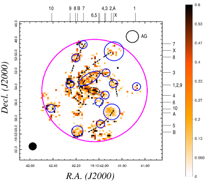
Figure 5: Map of the internal host-galaxy reddening $E(B-V)$ (in magnitudes) calculated via the measured Balmer decrement. The circles have the same meaning as in Figs. 1 and 4. Also shown is the seeing disk (diameter 1 arcsec).

4.4 Star formation rate and star-forming regions

Star formation rates were calculated via the extinction-corrected H$\alpha$ emission-line flux following Murphy et al. (2011) who used Starburst99 (Leitherer et al. 1999) and a Kroupa IMF (Kroupa 2001). According to these authors,

$$\mbox{SFR(H}\alpha)=5.37\times 10^{-42}\ L(\rm H\alpha)\ M_{\odot}\ \mbox{yr}^{-1}\,,$$ (2)

where the H$\alpha$ luminosity $L$ is measured in units of erg  s^-1.

The SFR map reveals several star-forming regions close to the central bar (see also Fig. 7) and scattered along the spiral arms up to about 15 kpc distance from the center of the galaxy (Fig. 6). All these regions can also be identified on the HST image (Fig. 1). In particular, the outer south-western arm pops up as a place with a high star formation activity (region A), in contrast to the outer northeastern arm, which shows comparably weak star formation activity (regions #7-9).

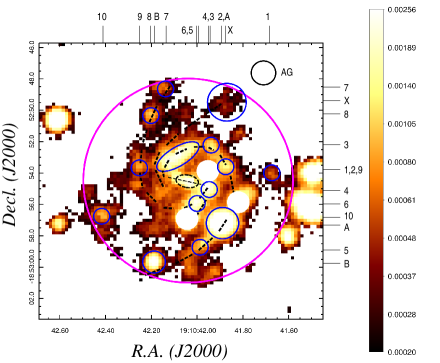
Figure 6: Map of the extinction-corrected star formation rate (for each spaxel in units of $M_{\odot}$ yr^-1). The circles have the same meaning as in Figs. 1 and 4. Compared to Fig. 5, here also regions with an adopted $E(B-V)=0$ are plotted. Similar to Fig. 4, outside the larger circle (in magenta), residual flux from bright Galactic foreground stars is seen. Only spaxels with an S/N$\geq 5$ in the measured SFR are plotted here.

The H$\alpha$-brightest star-forming region (designated A) lies about 10 arcsec (22 kpc) away from the afterglow position and about 3$\farcs$4 (7.6 kpc) away from the galaxy’s central bar. It has a bright, morphologically resolved counterpart on the HST/F606W image (Fig. 7). For this region, we measure a H$\alpha$ luminosity of about $5\,\times\,10^{40}$ erg s^-1 within a circle with a radius of 1$\farcs$0 (2.25 kpc). This corresponds to an extinction-corrected SFR of about 0.30 $M_{\odot}$ yr^-1 (Table 2).

When compared to the other star forming regions (Fig. 5), region A shows the lowest amount of reddening by dust. A trend of a decreasing reddening with increasing H$\alpha$ luminosity has been found in star-forming regions in other galaxies and supports a scenario in which the dust is destroyed or swept up by the intense radiation field of the most massive stars (e.g., Cairós & González-Pérez 2017).

Figure 8 shows the MUSE spectrum of region A, averaged over a region with a radius of 1^′′ (79 spaxels). Identified emission lines are labeled (for the laboratory wavelengths in air see Kramida et al. 2020).

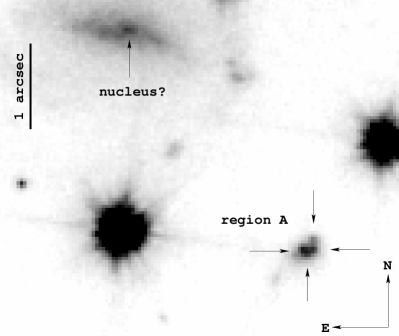
Figure 7: Zoom-in into the HST/F606W image (Fig. 1) at the position of the H$\alpha$-bright star-forming region A. It consists of at least four individual bright knots, tightly packed together within an area with a diameter of 0$\farcs$3-0$\farcs$4 ($\sim$0.7-0.9 kpc). Also indicated is a bright spot in the central bar of the galaxy, probably the luminous galactic nucleus.

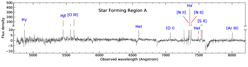
Figure 8: MUSE spectrum (gas cube; Sect. 3.2) of the most luminous star forming region (A) in the GRB 080905A host galaxy. The flux density is given in units of $10^{-20}$ erg s^-1 cm^-2 Å^-1 The most prominent emission lines are indicated: [O iii] stands for the lines at 4958.9 and 5006.8 Å, [N ii] for the lines at 6548.1 and 6583.4 Å, and [S ii] for the lines at 6716.4 and 6730.8 Å. The absorption features near 6550, 6850, and 7600 Å are of telluric origin. Note that we have split the spectrum into two parts in order to show the peaks of the bright and the faint emission lines.

No obvious H$\alpha$ line emission is detected from the area that contains (in projection) the GRB explosion site (black circle in Fig. 6). The GRB progenitor exploded in an environment that is apparently less filled with line-emitting gas. In this area, we find SFR(H$\alpha$)$<$0.003 $M_{\odot}$ yr^-1(3$\sigma$), measured in a region with the diameter of the seeing disk (1 arcsec).

The H$\alpha$ emission region that is closest to the position of the optical afterglow is region X, an isolated island (black circle in Fig. 1) at central coordinates R.A., decl. (J2000) = 19:10:41.87, $-$18:52:49.5. It lies about 2$\farcs$9 (6.5 kpc) away from the center of the afterglow error circle. Line emission from its outskirts can be followed up to a distance as close as 1$\farcs$7 (3.8 kpc) to the central afterglow position (Rowlinson et al. 2010). Region X shows a H$\alpha$ luminosity that corresponds to an SFR of $\sim$0.03 $M_{\odot}$ yr^-1 (Table 1) within a circle with a radius of 1$\farcs$2 (2.7 kpc). Contrary to the star-forming regions listed in Table 1, this is an area of diffuse H$\alpha$ emission with no centrally dominant peak.

For the entire galaxy we find a H$\alpha$ luminosity of about $2.6\,\times\,10^{41}$ erg s^-1 (Appendix A), corresponding to an extinction-corrected SFR of about 1.6 $M_{\odot}$ yr^-1 inside a circle with a radius of 6$\farcs$5 (15 kpc, Table 2) centered at the central bar of the host. Given this SFR and the mass estimate from Rowlinson et al. (2010), the specific SFR is about 1$\,\times\,10^{-10}$ yr^-1. For short-GRB hosts, this is a typical value (Berger 2014).

An SFR(H$\alpha$) of $\sim$1.6 $M_{\odot}$ yr^-1 has to be compared with the upper limit obtained from the ATCA observations (Sect. 3.1). Following Greiner et al. (2016), the constraint on the SFR is strongest for the 5.5 GHz data. For a Briggs robust parameter of 0.5, this leads to an SFR(radio) $<$1.1 $M_{\odot}$ yr^-1 per beam. Given that several beam sizes are required to cover the entire GRB 080905A host, the radio upper limit is consistent with the H$\alpha$-derived SFR.

4.5 Metallicity

In order to calculate the nebular oxygen abundance, we followed Pettini & Pagel (2004, PP04), according to whom the nebular oxygen abundance can be calculated as

$$12+\log\mbox{(O/H)} = 8.73-0.32\times\mbox{O3N2}\,,\,\,\,\mbox{with}$$ (3)

O3N2 $$\equiv \log\frac{\mbox{[O\,{\sc iii}]~{}$\lambda$}5007/\mbox{H}\beta}{\mbox{[N\,{\sc ii}]~{}$\lambda$}6584/\mbox{H}\alpha}\,\,.$$

In Fig. 9 we plot only spaxels for which S/N$\geq$2 simultaneously in H$\alpha$, [O iii] $\lambda$5007, H$\beta$, and [N ii] $\lambda$6584. Spaxels for which the flux ratio H$\alpha$/H$\beta$ was smaller than 2.86 are not plotted here.

Similarly to the reddening map, the metallicity map based on the PP04 formulation traces the spiral structure of the galaxy. What is immediately apparent in Fig. 9 is the metallicity gradient from the center of the galaxy to its outer regions. In addition, the star-formation sites A and B reveal themselves as large metal-poor regions (Table 2). In region A the mean of 12+log(O/H) is about 8.46, corresponding to $Z/Z_{\odot}$ = 0.59.

The metallicity is highest close to the galaxy’s bar, where 12+log(O/H) reaches the solar value. For the entire galaxy we measure a mean of $8.52\pm 0.01\ (Z/Z_{\odot}=0.68\pm 0.01)$. These results are in good agreement with VLT/FORS1 long-slit spectroscopy (Rowlinson et al. 2010). In particular, the apparent north-south asymmetry in the metallicity of the galaxy found by these authors turns out to be a consequence of the dominating nature of the giant, metal-poor, star-forming region A in the southern spiral arm.

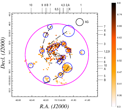
Figure 9: Map of the O3N2 metallicity indicator, given as 12 + log(O/H). The circles have the same meaning as in Figs. 1 and 4.

Table 2: Calculated Mean Values for the Brightest Star-forming Regions.

region	$E(B-V)$	SFR	Metallicity
	mag	0.01 $M_{\odot}$ yr-1	12+log(O/H)
A	0.08$\pm$ 0.01	31.0$\pm$1.4	8.46$\pm$ 0.01
B	0.14$\pm$ 0.06	6.5$\pm$1.2	8.36$\pm$ 0.03
D	0.19$\pm$ 0.05	13.8$\pm$2.0	8.67$\pm$ 0.02
bar; C	0.45$\pm$ 0.11	10.2$\pm$3.3	8.62$\pm$ 0.05
X	0.21$\pm$ 0.15	5.4$\pm$2.6	8.39$\pm$ 0.07
galaxy	0.04$\pm$ 0.01	160.8$\pm$7.0	8.52$\pm$ 0.01

Note. — All but one value have been calculated using the measured total emission-line luminosities listed in Appendix A. The exceptional case is the mean metallicity in region C. Here most spaxels have a very low S/N in the [O iii] line. Therefore, we calculated the mean using those 6 spaxels for which S/N$>$2 is fulfilled in all four lines (Fig. 9). For comparison, we also provide the corresponding numbers for the central bar (C) and for the entire galaxy, after masking out residual flux from the three bright Galactic foreground stars. In addition, we give the corresponding numbers for the region which in projection lies closest to the GRB explosion site (X). We caution, however, that here all numbers have a relatively large error.

4.6 Equivalent Width of H$\alpha$

The EW(H$\alpha$) map was constructed using spaxels for which S/N(H$\alpha$)$\geq$4 (Fig. 10). The map reveals a number of interesting features. The equivalent width is lowest in the central bar (C) of the galaxy (between 7 and 10 Å). It is much higher along the spiral arms (e.g., around 20–50 Å in region D), and highest in region A, where it peaks at about 200 Å. In region X it shows a larger valley (EW(H$\alpha$) between 6 and 9 Å) but increases to 30 – 50 Å at its northern border. In regions #8 and #10 the scatter in EW(H$\alpha$) is relatively high, the median is 68 and 56 Å, respectively. For the entire galaxy (within the bigger circle), we measure a mean of 29 and a median of 23 Å (Table 1).

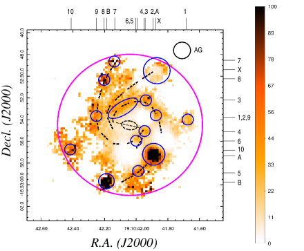
Figure 10: Map of the equivalent width EW(H$\alpha$) in units of Å. The star-forming regions A and B stand out here because of their very high EW values. The circles have the same meaning as in Figs. 1 and 4.

In order to interpret these results, we made use of the Starburst99 synthesis model (Leitherer et al. 1999). Its publicly available database provides a relationship between EW and the age of a star-forming region for three different initial mass functions (IMFs) and five metallicities between $Z$=0.040 and 0.001. Using this database, for the metallicities of interest here ($Z$= 0.009 – 0.020; Table 2), all star-forming regions have an age between 6 and 8 Myr; the results for different IMFs differ by at most 0.2 Myr. Nevertheless, other stellar population models like BPASS (Eldridge et al. 2017) can lead to older age estimates (e.g., Kuncarayakti et al. 2013, 2016). For example, for single stellar-evolution models, the age range for $Z$=0.009-0.020 for EW(H$\alpha$)=30-60 Å is 8-12 Myr. In particular, binary stellar-evolution models, which within the same metallicity and EW range, give an age range of 20-40 Myr. We do not investigate this further.

The trigger of the recent star-forming activity in the suspected host of GRB 080905A is still unclear. As noted above, in the data presented here we do not see evidence for any galaxy-galaxy interaction. Future HI 21 cm or other atomic and molecular line observations could be a promising tool to address this question (e.g., Arabsalmani et al. 2015; Michałowski et al. 2015, 2016, 2018, 2020; Hatsukade et al. 2020).

4.7 Emission-line Diagnostic Diagrams

We follow previous work (Nicuesa Guelbenzu et al. 2021) and use diagnostic Baldwin-Philips-Terlevich (BPT) emission-line diagrams (Baldwin et al. 1981) based on the line ratios [O iii] $\lambda$5007/H$\beta$ vs. [N ii] $\lambda$6584/H$\alpha$ and [O iii] $\lambda$5007/H$\beta$ vs. [S ii] $\lambda$6718/H$\alpha$ to distinguish between stellar ionization of the gas ([H ii]; star forming) and other ionization processes (stellar winds, AGN activity, shocks). In Fig. 9 we plot only spaxels for which S/N$\geq$2 simultaneously in all four lines. Spaxels that include residual light from the three Galactic foreground stars have been masked out here.

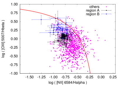
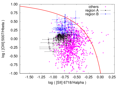
Figure 11: Emission-line Baldwin-Philips-Terlevich (BPT) diagnostic diagrams of the host of GRB 080905A. Left: diagnostic diagram using [N ii]. Shown are the corresponding values for all individual spaxels. Black data points refer to spaxels that lie inside region A; blue-colored data points refer to region B. For the sake of clarity, for these data points the corresponding $1\sigma$ error bars are also shown. The red line shows the pure star-formation demarcation line for a $z$=0.1218 galaxy (Kewley et al., 2013, their Equation 1). Right: The same as left but using [S ii] (Kewley et al. 2001 and Kewley et al. 2006; their Equations 6 and 2, respectively.).

Figure 11 shows the loci in the BPT diagrams of the regions with line emission in the GRB 080905A host galaxy. In both diagnostic diagrams, the majority of spaxels fall inside the parameter space characteristic of pure star formation. In the [N ii] diagram, star forming region A occupies a nearly circular area centered at the line ratios $(-0.780\pm 0.006,+0.036\pm 0.006)$; in the [S ii] diagram, the center of A has line ratios $(-0.827\pm 0.008,+0.027\pm 0.006)$. This clustering is also seen in the [S ii] diagram even though the spread in data points is a little larger. Not surprisingly, region A lies in the pure star formation area of the diagrams. For the other star-forming regions labeled in Fig. 1 there are significantly fewer data points and the clustering is less pronounced. Therefore, as an example in (Fig. 11) we only show region B.

4.8 The Suspected Background Galaxy Close to the OT

Using a circle with the diameter of the seeing disk (1 arcsec), at the position of the suspected faint background galaxy mentioned by Fong & Berger (2013) at R.A., decl. (J2000) = 19:10:41.743, $-$18:52:48.15 ($\pm$0$\farcs$05; Sect. 2.3), we detect emission from the redshifted H$\alpha$ line at $z$=0.1218, i.e., at the redshift of the large, barred spiral galaxy. There is also evidence for two faint emission lines close to H$\alpha$  centered at 7340 and 7402 Å ($\pm$0.5 Å). Unfortunately, the nature of these two lines could not be clarified. However, their origin in the suspected background object is unlikely. The first emission-line feature is also detected close to star-forming region A and the second feature close to B. This is about 9$\farcs$2 and 13$\farcs$2, respectively, away from the much less extended background object.

5 Discussion

Compared to the short-GRB host-galaxy ensemble listed in Berger (2014, his Table 2), an SFR of $\sim$1.6 $M_{\odot}$ yr^-1places the host of GRB 080905A in the middle of a rather broad distribution with SFR values between $<$0.1 and $>$10 $M_{\odot}$ yr^-1. Also with respect to metallicity, the galaxy is a rather normal short-GRB host.

Even though the global SFR of the GRB 080905A host is rather modest, the MUSE data have revealed several star-forming complexes scattered across the galaxy. Particularly striking is the giant star-forming region A which is responsible for $\sim$20% of the SFR of the entire galaxy and shines like a bright lighthouse in the H$\alpha$ line. On the HST image, its diameter is approximately twice the extension of the Tarantula nebula (30 Doradus; diameter 370 pc) in the LMC (Crowther 2019), while its H$\alpha$ luminosity is nearly four times as high.

The high-resolution HST image suggests that the angular size of this banana-shaped region is only about 0$\farcs$3-0$\farcs$4 at its longest (NW–SE) extension ($\sim$0.7-0.9 kpc) and consists of at least four individual knots (Fig. 7). The star formation rate surface density $\Sigma_{\rm SFR}$ in this region is about 0.5-0.8 $M_{\odot}$ yr^-1 kpc^-2. In the VLT/MUSE data cube, this region cannot be spatially resolved.

To some degree, region A and its relation with its host resembles the Wolf–Rayet star-forming region in the GRB 980425 host galaxy – very bright in H$\alpha$ and a strong radiation field (Christensen et al. 2008; Michałowski et al. 2014, 2016; Krühler et al. 2017). GRB 980425 was a long burst, however; its origin was the collapse of a massive star. In any case, very detailed studies of long-GRB-hosts with VLT/MUSE (e.g., GRB 980425: Krühler et al. 2017; GRB 100316D: Izzo et al. 2017; GRB 111005A: Tanga et al. 2018) but also of the hosts of various supernovae (e.g., Chen et al. 2017; Galbany et al. 2016; Sun et al. 2021) have revealed a plethora of information about the star-formation activity in dwarf and spiral galaxies.

The center of region A lies about 10^′′ (22 kpc) in projection away from the GRB explosion site. Several other, but less luminous star-forming regions are located at much closer distance to the afterglow position. Could any of these star-forming regions be the original birthplace of the short-GRB progenitor? In order to tackle this question, we made use of an available set of stellar population synthesis calculations.

5.1 The Stellar Population Synthesis Code

We employed the population synthesis code StarTrack (Belczynski et al., 2002, 2008) to obtain astrophysically motivated physical properties of NS–NS binaries. We adopted the rapid core-collapse supernova engine NS/BH mass calculation (Fryer et al., 2012) that allows for NS formation in a mass range $1-2.5~{}M_{\odot}$. Natal kicks NSs/BHs have received at formation are taken from a one-dimensional Maxwellian distribution with $\sigma=265$ km s^-1 (Hobbs et al. 2005) and were decreased inversely proportionally to the amount of fallback calculated for each supernova event (Fryer et al., 2012). This procedure was applied to NSs formed in core-collapse supernovae. However, for NSs formed in electron-capture supernovae, we did not apply a natal kick. Blaauw kicks (from a symmetric mass loss; Blaauw 1961; Repetto et al. 2012) were applied to all NSs. We assumed standard wind losses for massive stars: O/B star (Vink et al. 2001) winds and LBV winds (specific prescriptions for these winds are listed in Sect. 2.2 of Belczynski et al., 2010). We treated accretion onto a compact object during Roche lobe overflow and from stellar winds using the analytic approximations presented in King et al. (2001); Mondal et al. (2020). We adopted a limited 5% Bondi accretion rate onto BHs/NSs during common envelope (Ricker & Taam, 2008; MacLeod et al., 2017). The most updated description of StarTrack is given in Belczynski et al. (2020). Here we use the input physics from model M30 of that paper. Model 30 was used as it employs optimal input physics assumptions on stellar and binary evolution as argued in Belczynski et al. (2020).

The numerical code delivers the NS masses, the time of their formation (starting at ZAMS at $t$=0), the type of SN, the time between the two SNe, the velocity vector of the binary after the first ($t=t_{1}$) and after the second SN ($t=t_{2}$), and the time from the second SN to the merger ($t=t_{3}$; Table 3). In other words, after the first SN the system will begin moving in one direction for a time span $t_{2}-t_{1}$. After the second supernova, the binary will start moving in some other direction for a time span $t_{3}-t_{2}$.

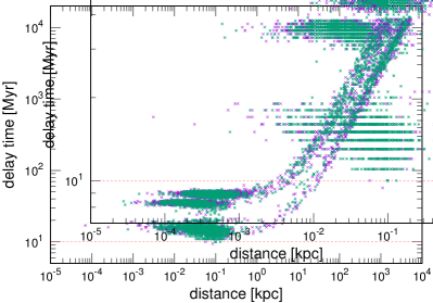
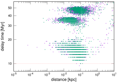
Figure 12: Top: delay time versus spatial distance from the stellar nursery for the stellar population models considered here (green: model M30, 3696 simulations; violet: model M35, 4633 simulations). All but 1 NS–NS system are characterized by a delay time of more than 10 Myr (red line). Bottom: zoom-in into the upper figure to better show the systems with the shortest delay times. For the exceptional case with a delay time of 9.43 Myr, see Sect. B.

Table 3: The Stellar Population Synthesis Model.

Time	Distance	Comment
$t$=0	$d$=0	ZAMS
$t=t_{1}$	$d=d_{1}$=0	1st SN
$t=t_{2}$	$d=d_{2}$	2nd SN
$t=t_{3}$	$d=d_{3}$	merger

Note. — The stellar population synthesis (SPS) model: the time difference $t_{3}-t_{2}$ is the merger time $t_{\rm mr}$. The delay time, however, is defined as the time from arrival at the ZAMS ($t$=0) to the merger: $t_{\rm delay}$ = max$(t_{1},t_{2})+t_{\rm mr}$. $d$ is the spatial distance from the stellar nursery.

Natal kicks and their mechanism are not fully understood or observationally constrained, so, in order to fully assess this uncertainty, one way could be to consider two extreme models: no natal kicks and maximum (very hard to assess what is actual maximum) natal kicks (which are estimated at about $>$1000 km s^-1). This does not really need to be shown, as no natal kicks would result in travel distance close to 0 kpc (there would be a small systemic velocity increase due to a symmetric mass loss at NS formation), while for kicks as high as 1000 km s^-1 there would be virtually no NS–NS progenitors surviving. We propose to do a different sort of possibly more realistic exercise: if NSs in binaries receive kicks, it is claimed that they receive possibly smaller kicks than single pulsars (Willems et al. 2008 and references therein). Therefore, we also considered one more model, exactly the same as M30, but with 50% natal kicks ($\sigma$ = 130 km s^-1; model M35). Figure 12 shows the arising difference/uncertainty. It also shows that in all but one case, all NS–NS mergers are characterized by a delay time larger than 10.0 Myr. The single exceptional case is an NS–NS system in model M30 with a delay time of 9.43 Myr (Sect. B).

5.2 Linking the Model Results to the Host of the Short GRB 080905A

Before applying the results of the numerical BNS population synthesis model to the host case discussed here, we describe some specifics of the assumed star-formation history. Following Leitherer et al. (1999), we distinguish two scenarios.

5.2.1 The Instantaneous Starburst Scenario

Here we assume that all currently detectable H$\alpha$-bright star-forming regions are the result of a single instantaneous starburst. Within this scenario, all stars arrived at the ZAMS at $t$=0. Then, after a while, SNe start to explode and compact stellar binaries (NS–NS) begin to form and finally merge at a certain spatial distance $d$ from the stellar birthplace (Table 3).

Within the context of this model, the evolutionary state of a star-forming region as a luminous H$\alpha$ source lasts less than 6-10 Myr (e.g., Copetti et al. 1986; Tremblin et al. 2014). As we have outlined in Section 4.6, using the the Starburst99 database (Leitherer et al. 1999), all star-forming regions listed in Table 1 have an age between 6 and 8 Myr.

The numerical modeling presented in Sect. 5.1 shows that very special circumstances are required so that an NS–NS merger can occur within a delay time of less than 10 Myr (see Sect. B). We thus conclude that it is theoretically possible but statistically not likely that an NS–NS binary merges already within 10 Myr after the arrival of its two progenitor stars on the ZAMS. This conclusion is insensitive to the adopted metallicity of the star-forming region.

Adding to our model BH–NS mergers would not make any difference to these conclusions. (i) Their formation is less frequent than the formation of NS–NS systems (see Table 3 and 4 in Belczynski et al. 2020 for model M30). (ii) Only a small fraction of BH–NS mergers are predicted to produce mass ejecta that would power a GRB (see Drozda et al. 2020; BH–NS mergers with ejecta represent only $<$10% of entire merging BH–NS population). Very special conditions are required such as a high BH spin and comparable masses of BH and NS to produce mass ejecta in BH–NS mergers.

We can go one step further and assume that our age constraints that we derived from Starburst99 are wrong by 50%, i.e., we allow for stellar ages up to 12 Myr. Then, in model M30, altogether 23 systems fulfill this age criterion; in model M35 these are 69 binaries. However, if we also require that at the time of the merger the progenitor system has traveled at least 3 kpc from its birthplace, none of the binaries satisfy this criterion. All NS–NS systems with short delay times have travel distances between 0.06 and 0.18 kpc (model M30) and, respectively, 0.02 and 0.36 kpc (model M35). This stems from the fact that the shortest-lived NS–NS systems cannot travel too far even if they acquired high systemic speeds from natal kicks and/or SN mass loss. In other words, taking into account the age and the distance constraints, none of the simulated mergers allows for a link of the merger progenitor to any of the presently active star-forming regions listed in Table 1. Within the context of the instantaneous starburst scenario (Leitherer et al. 1999), none of these regions is a likely birthplace of the short-GRB progenitor system.

We finally note that even within the context of the instantaneous starburst scenario, our MUSE observations do not exclude the potential existence of star-forming regions older than 10 Myr. However, for such ages, H$\alpha$ is no longer a good tracer of star-forming activity. A deep UV imaging of the suspected GRB 080905A host galaxy could reveal older star-forming complexes, but no such data are at hand.

5.2.2 The Continuous Star Formation Scenario

In such a case, the interpretation of observational data becomes much more complex. In this scenario, EW(H$\alpha$) basically remains constant and at a high level as long as the starburst holds on (e.g., Kuncarayakti et al. 2013, their figure 1). For example, if we increase the constraint on the age of the short-GRB progenitor to 100 Myr, then 82% of the modeled evolutionary tracks predict an NS–NS merger within such a time span. However, only a small fraction (2%) of these NS–NS mergers with delay times below 100 Myr have travel distances larger than 3 kpc.

5.2.3 Binary Stellar Population Models

Starburst99 is based on single-star evolutionary tracks. Observations suggest, however, that most massive stars are born in binaries (e.g., Sana et al. 2012). Moreover, the progenitor of GRB 080905A might have been a tight binary. This suggests that for EW(H$\alpha$) age estimates, binary stellar population models should be considered too.

Xiao et al. (2019) used the BPASS (binary population spectral and synthesis) models (Eldridge et al. 2017) to investigate the EW(H$\alpha$)-age-metallicity relationship and compared their results with single-star evolution models. They found that binary models can predict a much larger age once EW(H$\alpha$)$\lesssim$1000 Å; and this holds for all metallicities $Z\gtrsim 0.001$. This age difference increases with decreasing EW (see also Lyman et al. 2018, their figure 4). For $Z$=0.009–0.020 and EW(H$\alpha$)=30–60 Å, the predicted age range of the BPASS model is 20–40 Myr, compared to about 8–12 Myr for single-star models (Kuncarayakti et al. 2016, their figure 1).

We find that in model M30 and in model M35, less than 1% of all NS–NS mergers have delay times smaller than 30 Myr and travel distances larger than 3 kpc. Similarly to the continuous star formation model, the probability is low that the GRB progenitor fits into this scenario even though it is clear that binary models can bring a new flavor into the question we have touched here. Going further into these models might be an option for further studies. Discussing this issue in detail is, however, beyond the scope of this paper.

6 Summary

By combining archival HST data (program ID 12502; PI: A. Fruchter) with VLT/MUSE observations, we have explored the star-formation properties of the host of the short GRB 080905A. The MUSE data allowed us to explore its internal extinction, star forming activity, metallicity, and its radial velocity pattern.

Using H$\alpha$ emission as a tracer for star formation, we found that the host contains several luminous star-forming complexes scattered across its spiral arms. Star formation activity can be found throughout the galaxy disk. The closest star-forming region to the GRB explosion site is about 3 kpc (in projection) away. For the entire galaxy, we measure a H$\alpha$ SFR of about 1.6 $M_{\odot}$ yr^-1.

The largest and most luminous star-forming complex (labeled A; Fig. 1) lies 22 kpc in projection away from the GRB afterglow position. It shows a H$\alpha$ luminosity of about $5\,\times\,10^{40}$ erg s^-1 and has a star formation rate surface density $\Sigma_{\rm SFR}$ on the order of about 0.5–0.8 $M_{\odot}$ yr^-1per kpc². This is a high value and comparable to what has been found in luminous infrared galaxies (Piqueras López et al. 2016).

For all star-forming regions, including region A, we measure an H$\alpha$ equivalent width that suggests individual ages of less than 10 Myr, provided that all star-forming activity has its origin in single instantaneous starbursts. Within this context, our stellar population synthesis calculations show that none of these H$\alpha$-bright star-forming regions can be considered as a candidate stellar nursery that has formed the NS–NS progenitor.

Appendix A Additional Tables

Table 4 provides for all regions indicated in Fig. 1 the measured luminosities in the five emission lines.

Table 4: Measured Emission-line Luminosities (in Units of 10³⁹ erg s^-1) for the Regions Indicated in Figure 1.

Region	$L$(H$\alpha$)	$L$(H$\beta$)	$L$([O iii] $\lambda$5007)	$L$([N ii] $\lambda$6584)	$L$([S ii] $\lambda$6718)
A	45.20 $\pm$ 0.22	14.40 $\pm$ 0.23	12.60 $\pm$ 0.22	5.77 $\pm$ 0.21	5.14 $\pm$ 0.21
B	7.86 $\pm$ 0.15	2.33 $\pm$ 0.15	3.25 $\pm$ 0.15	0.79 $\pm$ 0.14	1.04 $\pm$ 0.14
C	4.81 $\pm$ 0.12	1.05 $\pm$ 0.12	0.15 $\pm$ 0.11	1.45 $\pm$ 0.11	1.06 $\pm$ 0.11
D	14.40 $\pm$ 0.21	4.04 $\pm$ 0.21	1.31 $\pm$ 0.20	3.12 $\pm$ 0.19	2.54 $\pm$ 0.20
X	5.26 $\pm$ 0.25	1.44 $\pm$ 0.25	1.70 $\pm$ 0.25	0.52 $\pm$ 0.24	0.80 $\pm$ 0.24
1	1.63 $\pm$ 0.10	0.57 $\pm$ 0.10	0.66 $\pm$ 0.10	0.12 $\pm$ 0.10	0.32 $\pm$ 0.10
2	4.27 $\pm$ 0.11	1.62 $\pm$ 0.11	0.70 $\pm$ 0.11	0.80 $\pm$ 0.10	0.71 $\pm$ 0.10
3	3.09 $\pm$ 0.11	0.97 $\pm$ 0.11	0.51 $\pm$ 0.10	0.53 $\pm$ 0.10	0.54 $\pm$ 0.10
4	6.92 $\pm$ 0.11	2.38 $\pm$ 0.11	0.74 $\pm$ 0.10	1.48 $\pm$ 0.10	1.10 $\pm$ 0.10
5	2.75 $\pm$ 0.11	0.87 $\pm$ 0.11	0.85 $\pm$ 0.10	0.36 $\pm$ 0.10	0.52 $\pm$ 0.10
6	6.15 $\pm$ 0.11	3.21 $\pm$ 0.11	0.88 $\pm$ 0.11	1.26 $\pm$ 0.10	0.85 $\pm$ 0.10
7	1.77 $\pm$ 0.11	0.61 $\pm$ 0.11	1.05 $\pm$ 0.10	0.10 $\pm$ 0.10	0.19 $\pm$ 0.10
8	2.54 $\pm$ 0.11	0.75 $\pm$ 0.11	0.85 $\pm$ 0.10	0.25 $\pm$ 0.10	0.32 $\pm$ 0.10
9	2.14 $\pm$ 0.11	0.46 $\pm$ 0.11	0.32 $\pm$ 0.10	0.43 $\pm$ 0.10	0.38 $\pm$ 0.10
10	2.42 $\pm$ 0.11	0.94 $\pm$ 0.11	0.79 $\pm$ 0.10	0.30 $\pm$ 0.10	0.36 $\pm$ 0.10
galaxy	264.00 $\pm$ 1.38	88.00 $\pm$ 1.37	59.60 $\pm$ 1.33	40.90 $\pm$ 1.32	42.10 $\pm$ 1.32

Note. — The luminosities are based on all spaxels which fulfill the criterion S/N$\geq$2 in the corresponding line. The data for the entire galaxy exclude the flux coming from masked regions that cover the three bright Galactic foreground stars (Fig. 1). With the exception of H$\beta$, for these three regions we used a mask with a radius of 0$\farcs$7. In the case of H$\beta$, for the two stars next to region A we had to increase the radius of the mask to 0$\farcs$9; for the third star next to regions #2 and #4 we still used 0$\farcs$7, however. The error includes the r.m.s. of the corresponding luminosity, measured in an area with the diameter of the seeing disk (1 arcsec) in various regions around the galaxy and added in quadrature to the measurement error. For all lines this $1\sigma_{\rm rms}$ error was about $10^{37}$ erg s^-1.

.

Appendix B An NS–NS Model With a Delay Time of Less than 10 Myr

In the SPS model outlined in Sect. 5.1, the minimum timescale is set by the time the two massive stars need to evolve from the ZAMS to the formation of two NSs. The time needed for the two NSs to merge (due to gravitational wave emission) may be very short for very close (common envelope) and highly eccentric orbits (natal kick). The evolutionary time is set by the stellar mass. In our models single stars with a mass below $\sim 20$ $M_{\odot}$ form NSs while heavier stars form BHs. The evolution of a 20 $M_{\odot}$ star takes $\sim 10.5$ Myr. Binary evolution may in exceptional cases act in such way as to produce NS–NS mergers at timescales below 10 Myr. In our particular case of an NS–NS merger with a delay time of 9.4 Myr, this is exactly what happens.

The binary system starts with two massive stars above the NS formation mass limit: 22.34 $M_{\odot}$ and 22.33 $M_{\odot}$ at ZAMS. Note that these stars have virtually the same mass which is unusual as our initial binary population has a uniformly distributed mass ratio. The more massive star (primary) begins Roche lobe overflow (RLOF) on a thermal timescale right after leaving the main sequence and a large fraction of its envelope is lost from the binary. Soon after, the less massive star (secondary) also expands beyond its Roche lobe and initiates a common envelope (CE) that removes its H-rich envelope and whatever is left from the H-rich envelope of the primary star. Then at a time $t=9.1$ Myr, the secondary explodes in a core-collapse SN forming a more massive NS in the system: 1.84 $M_{\odot}$ . Note two things: (i) the secondary explodes first due to a mass ratio reversal caused by mass accretion from the primary during RLOF, and (ii) NS formation happens below $t$=10 Myr due to the fact that the main-sequence evolution timescale was well below that of the most massive single star that can form an NS. Shortly after, the primary expands again and as a helium giant initiates yet another CE phase, it loses its entire He-rich envelope. At this point, it lost enough mass so that it also forms an NS with a mass of 1.44 $M_{\odot}$ and the second supernova happens at $t=9.4$ Myr. At this point, the system is very compact (after two CE phases) so that it may easily survive even a large natal kick that will induce significant eccentricity to the NS–NS binary without disrupting the system. This significantly reduces the merger time. The final NS–NS semi-major axis is very small ($a=0.3$ $R_{\odot}$) and eccentric ($e=0.6$) and that translates to a merger time of only 0.03 Myr. Therefore, it takes only 9.43 Myr from ZAMS to the NS–NS merger and the GRB. The combination of very high stellar masses and the fact of both masses being virtually equal sends the system on the very unique evolutionary trajectory generating a very short delay time.

Appendix C ATCA Constraints on GRB Late-time Emission Components

The ATCA radio observations constrain the luminosity of any long-lived radio transient related to the burst. This refers to the luminosity of the radio afterglow (e.g., Chandra & Frail 2012) and to a potential late-time kilonova radio flare (Nakar & Piran 2011; Metzger & Bower 2014; Margalit & Piran 2015; Fong et al. 2016; Horesh et al. 2016; Radice et al. 2018).

Following the procedure outlined in Klose et al. (2019), and assuming an isotropically radiating source, the corresponding upper limits are listed in Table 5. Here, for the radio afterglow, we considered a spectral slope ($F_{\nu}\sim\nu^{-\beta}$) of $\beta=-1/3$ or 0.7 and for a kilonova radio flare, we set $\beta=0.7$.

Since our ATCA observations resulted in non-detections, we provide the corresponding upper limits on the luminosity based on multiples of the noise level on the radio image. In the Table we provide the measured $1\sigma$ r.m.s. in an area of $60^{\prime\prime}\times 60^{\prime\prime}$ centered at the target position for a robust parameter of 0.5. Following Klose et al. (2019) and Nicuesa Guelbenzu et al. (2021), we then calculated the corresponding radio luminosity upper limits of a point source by using five times this r.m.s. value. For the sake of clarity we note that using our data we could also claim $2\sigma$ luminosity upper limits. However, given the fact that these are interferometric data and the noise is not really Gaussian, we follow others (e.g., Wadadekar & Kembhavi 1999; Tasse et al. 2006; Stroe et al. 2012) and provide $5\sigma$ sensitivities. We refer to Murphy et al. (2017) for a more stringent discussion on this important issue.

Table 5: $5\sigma$ Upper Limits on Late-time Radiation Components.

Run	$dt_{\rm obs}$	$dt_{\rm host}$	$1\sigma_{\rm rms}$	$L_{\nu,1}$	$L_{\nu,2}$	$\nu L_{\nu,1}$	$\nu L_{\nu,2}$
(1)	(2)	(3)	(4)	(5)	(6)	(7)	(8)
Run 1, 5.5 GHz	4.87	4.34	12.6	2.2	2.5	1.2	1.4
9.0 GHz			15.4	2.7	3.0	2.4	2.7
Run 2, 5.5 GHz	7.13	6.36	6.7	1.2	1.3	0.6	0.7
9.0 GHz			8.6	1.5	1.7	1.4	1.5

Note. — Columns #2 and #3 give the time after the burst in the observer and in the host frame, respectively. Column #4 contains the 1$\sigma$ r.m.s. on the radio image. Columns #5 to #8 provide the corresponding 5$\sigma$ upper limits (in units of $\mu$Jy beam^-1) for the specific luminosity $L_{\nu}$ (in units of $10^{28}$ erg s^-1 Hz^-1) as well as for $\nu L_{\nu}$ (in units of $10^{38}$ erg s^-1), assuming isotropic emission. $L_{\nu,1}$ assumes a spectral slope $\beta=-1/3$, $L_{\nu,2}$ assumes $\beta=0.7$.

The non-detection of the radio afterglow is not surprising given the statistics of the observed luminosities of radio afterglows from short GRBs (Chandra & Frail 2012; Fong et al. 2015). The non-detection of a late-time radio flare is in the line with other unsuccessful searches for such signatures (Metzger & Bower 2014; Fong et al. 2016; Horesh et al. 2016; Klose et al. 2019; Ricci et al. 2021; Schroeder et al. 2020). For a detailed theoretical discussion of these non-detections we refer to recent papers by Margalit & Piran (2020) and Liu et al. (2020).

References

- Abbott et al. (2017) Abbott, B. P., Abbott, R., Abbott, T. D., et al. 2017, ApJ, 848, L12
- Arabsalmani et al. (2015) Arabsalmani, M., Roychowdhury, S., Zwaan, M. A., Kanekar, N., & Michałowski, M. J. 2015, MNRAS, 454, L51
- Asplund et al. (2009) Asplund, M., Grevesse, N., Sauval, A. J., & Scott, P. 2009, ARA&A, 47, 481
- Atteia et al. (1987) Atteia, J. L., Barat, C., Hurley, K., et al. 1987, ApJS, 64, 305
- Bacon et al. (2010) Bacon, R., Accardo, M., Adjali, L., et al. 2010, in Society of Photo-Optical Instrumentation Engineers (SPIE) Conference Series, Vol. 7735, Ground-based and Airborne Instrumentation for Astronomy III, ed. I. S. McLean, S. K. Ramsay, & H. Takami, 773508
- Bacon et al. (2017) Bacon, R., Conseil, S., Mary, D., et al. 2017, A&A, 608, A1
- Baldwin et al. (1981) Baldwin, J. A., Phillips, M. M., & Terlevich, R. 1981, PASP, 93, 5
- Baron et al. (2018) Baron, D., Netzer, H., Prochaska, J. X., et al. 2018, MNRAS, 480, 3993
- Barthelmy et al. (2005) Barthelmy, S. D., Barbier, L. M., Cummings, J. R., et al. 2005, Space Sci. Rev., 120, 143
- Belczynski et al. (2010) Belczynski, K., Bulik, T., Fryer, C. L., et al. 2010, ApJ, 714, 714
- Belczynski et al. (2002) Belczynski, K., Kalogera, V., & Bulik, T. 2002, ApJ, 572, 572
- Belczynski et al. (2008) Belczynski, K., Kalogera, V., Rasio, F. A., et al. 2008, ApJS, 174, 174
- Belczynski et al. (2020) Belczynski, K., Klencki, J., Fields, C. E., et al. 2020, A&A, 636, A104
- Berger (2014) Berger, E. 2014, ARA&A, 52, 43
- Bissaldi et al. (2008) Bissaldi, E., McBreen, S., Connaughton, V., & von Kienlin, A. 2008, GRB Coordinates Network, 8204, 1
- Blaauw (1961) Blaauw, A. 1961, Bull. Astron. Inst. Netherlands, 15, 265
- Bloom et al. (1998) Bloom, J. S., Djorgovski, S. G., Kulkarni, S. R., & Frail, D. A. 1998, ApJ, 507, L25
- Bloom et al. (2006) Bloom, J. S., Prochaska, J. X., Pooley, D., et al. 2006, ApJ, 638, 354
- Boer et al. (1991) Boer, M., Hurley, K., Pizzichini, G., & Gottardi, M. 1991, A&A, 249, 118
- Briggs (1995) Briggs, D. S. 1995, in Bulletin of the American Astronomical Society, Vol. 27, American Astronomical Society Meeting Abstracts, #112.02
- Bruzual & Charlot (2003) Bruzual, G. & Charlot, S. 2003, MNRAS, 344, 1000
- Burrows et al. (2005) Burrows, D. N., Hill, J. E., Nousek, J. A., et al. 2005, Space Sci. Rev., 120, 165
- Cairós & González-Pérez (2017) Cairós, L. M. & González-Pérez, J. N. 2017, A&A, 600, A125
- Caplan & Deharveng (1986) Caplan, J. & Deharveng, L. 1986, A&A, 155, 297
- Chandra & Frail (2012) Chandra, P. & Frail, D. A. 2012, ApJ, 746, 156
- Chen et al. (2017) Chen, T.-W., Schady, P., Xiao, L., et al. 2017, ApJ, 849, L4
- Christensen et al. (2008) Christensen, L., Vreeswijk, P. M., Sollerman, J., et al. 2008, A&A, 490, 45
- Cid Fernandes et al. (2005) Cid Fernandes, R., Mateus, A., Sodré, L., Stasińska, G., & Gomes, J. M. 2005, MNRAS, 358, 363
- Cid Fernandes et al. (2009) Cid Fernandes, R., Schoenell, W., Gomes, J. M., et al. 2009, in Revista Mexicana de Astronomia y Astrofisica Conference Series, Vol. 35, Revista Mexicana de Astronomia y Astrofisica Conference Series, 127–132
- Copetti et al. (1986) Copetti, M. V. F., Pastoriza, M. G., & Dottori, H. A. 1986, A&A, 156, 111
- Coulter et al. (2017) Coulter, D. A., Foley, R. J., Kilpatrick, C. D., et al. 2017, Science, 358, 1556
- Crowther (2019) Crowther, P. A. 2019, Galaxies, 7, 88
- Cummings et al. (2008) Cummings, J., Barthelmy, S. D., Baumgartner, W., et al. 2008, GRB Coordinates Network, 8187, 1
- D’Avanzo et al. (2014) D’Avanzo, P., Salvaterra, R., Bernardini, M. G., et al. 2014, MNRAS, 442, 2342
- de Ugarte Postigo et al. (2008) de Ugarte Postigo, A., Malesani, D., Levan, A. J., Hjorth, J., & Tanvir, N. R. 2008, GRB Coordinates Network, 8195, 1
- Djorgovski et al. (1998) Djorgovski, S. G., Kulkarni, S. R., Bloom, J. S., et al. 1998, ApJ, 508, L17
- Domínguez et al. (2013) Domínguez, A., Siana, B., Henry, A. L., et al. 2013, ApJ, 763, 145
- Drozda et al. (2020) Drozda, P., Belczynski, K., O’Shaughnessy, R., Bulik, T., & Fryer, C. L. 2020, arXiv e-prints, arXiv:2009.06655
- Eldridge et al. (2017) Eldridge, J. J., Stanway, E. R., Xiao, L., et al. 2017, PASA, 34, e058
- Erroz-Ferrer et al. (2019) Erroz-Ferrer, S., Carollo, C. M., den Brok, M., et al. 2019, MNRAS, 484, 5009
- Evans et al. (2009) Evans, P. A., Beardmore, A. P., Page, K. L., et al. 2009, MNRAS, 397, 1177
- Evans et al. (2008) Evans, P. A., Osborne, J. P., & Goad, M. R. 2008, GRB Coordinates Network, 8203, 1
- Fong & Berger (2013) Fong, W. & Berger, E. 2013, ApJ, 776, 18
- Fong et al. (2015) Fong, W., Berger, E., Margutti, R., & Zauderer, B. A. 2015, ApJ, 815, 102
- Fong et al. (2016) Fong, W., Metzger, B. D., Berger, E., & Özel, F. 2016, ApJ, 831, 141
- Fruchter et al. (2006) Fruchter, A. S., Levan, A. J., Strolger, L., et al. 2006, Nature, 441, 463
- Fryer et al. (2012) Fryer, C. L., Belczynski, K., Wiktorowicz, G., et al. 2012, ApJ, 749, 749
- Galama et al. (1998) Galama, T. J., Vreeswijk, P. M., van Paradijs, J., et al. 1998, Nature, 395, 670
- Galbany et al. (2016) Galbany, L., Anderson, J. P., Rosales-Ortega, F. F., et al. 2016, MNRAS, 455, 4087
- Gehrels et al. (2004) Gehrels, N., Chincarini, G., Giommi, P., et al. 2004, ApJ, 611, 1005
- Gehrels et al. (2006) Gehrels, N., Norris, J. P., Barthelmy, S. D., et al. 2006, Nature, 444, 1044
- Gehrels et al. (2005) Gehrels, N., Sarazin, C. L., O’Brien, P. T., et al. 2005, Nature, 437, 851
- Greiner et al. (2008) Greiner, J., Bornemann, W., Clemens, C., et al. 2008, PASP, 120, 405
- Greiner et al. (2016) Greiner, J., Michałowski, M. J., Klose, S., et al. 2016, A&A, 593, A17
- Groot et al. (1997) Groot, P. J., Galama, T. J., van Paradijs, J., et al. 1997, IAU Circ., 6584, 1
- Groves et al. (2012) Groves, B., Brinchmann, J., & Walcher, C. J. 2012, MNRAS, 419, 1402
- Hammer et al. (2006) Hammer, F., Flores, H., Schaerer, D., et al. 2006, A&A, 454, 103
- Hatsukade et al. (2020) Hatsukade, B., Ohta, K., Hashimoto, T., et al. 2020, ApJ, 892, 42
- Hjorth et al. (2017) Hjorth, J., Levan, A. J., Tanvir, N. R., et al. 2017, ApJ, 848, L31
- Hjorth et al. (2005) Hjorth, J., Sollerman, J., Gorosabel, J., et al. 2005, ApJ, 630, L117
- Hobbs et al. (2005) Hobbs, G., Lorimer, D. R., Lyne, A. G., & Kramer, M. 2005, MNRAS, 360, 360
- Horesh et al. (2016) Horesh, A., Hotokezaka, K., Piran, T., Nakar, E., & Hancock, P. 2016, ApJ, 819, L22
- Hurley & Cline (1994) Hurley, K. & Cline, T. 1994, in American Institute of Physics Conference Series, Vol. 307, Gamma-Ray Bursts, ed. G. J. Fishman, 653
- Hurley et al. (1997) Hurley, K., Hartmann, D., Kouveliotou, C., et al. 1997, ApJ, 479, L113
- Hurley et al. (1993) Hurley, K., Sommer, M., Cline, T., et al. 1993, in American Institute of Physics Conference Series, Vol. 280, American Institute of Physics Conference Series, ed. M. Friedlander, N. Gehrels, & D. J. Macomb, 769–773
- Izzo et al. (2017) Izzo, L., Thöne, C. C., Schulze, S., et al. 2017, MNRAS, 472, 4480
- Jimmy et al. (2016) Jimmy, Tran, K.-V., Saintonge, A., et al. 2016, ApJ, 825, 34
- Joye & Mandel (2003) Joye, W. A. & Mandel, E. 2003, in Astronomical Society of the Pacific Conference Series, Vol. 295, Astronomical Data Analysis Software and Systems XII, ed. H. E. Payne, R. I. Jedrzejewski, & R. N. Hook, 489
- Kasen et al. (2017) Kasen, D., Metzger, B., Barnes, J., Quataert, E., & Ramirez-Ruiz, E. 2017, Nature, 551, 80
- Kewley et al. (2001) Kewley, L. J., Dopita, M. A., Sutherland, R. S., Heisler, C. A., & Trevena, J. 2001, ApJ, 556, 121
- Kewley et al. (2006) Kewley, L. J., Groves, B., Kauffmann, G., & Heckman, T. 2006, MNRAS, 372, 961
- Kewley et al. (2013) Kewley, L. J., Maier, C., Yabe, K., et al. 2013, ApJ, 774, L10
- Kewley et al. (2019) Kewley, L. J., Nicholls, D. C., & Sutherland, R. S. 2019, ARA&A, 57, 511
- Kim et al. (2017) Kim, S., Schulze, S., Resmi, L., et al. 2017, ApJ, 850, L21
- King et al. (2001) King, A. R., Davies, M. B., Ward, M. J., Fabbiano, G., & Elvis, M. 2001, ApJ, 552, L109
- Klose et al. (1996) Klose, S., Eisloeffel, J., & Richter, S. 1996, ApJ, 470, L93
- Klose et al. (2019) Klose, S., Nicuesa Guelbenzu, A. M., Michałowski, M. J., et al. 2019, ApJ, 887, 206
- Kramida et al. (2020) Kramida, A., Yu. Ralchenko, Reader, J., & and NIST ASD Team. 2020, NIST Atomic Spectra Database (ver. 5.8), [Online]. Available: https://physics.nist.gov/asd [2021, August 18]. National Institute of Standards and Technology, Gaithersburg, MD.
- Kroupa (2001) Kroupa, P. 2001, MNRAS, 322, 231
- Krühler et al. (2017) Krühler, T., Kuncarayakti, H., Schady, P., et al. 2017, A&A, 602, A85
- Kuncarayakti et al. (2013) Kuncarayakti, H., Doi, M., Aldering, G., et al. 2013, AJ, 146, 30
- Kuncarayakti et al. (2016) Kuncarayakti, H., Galbany, L., Anderson, J. P., Krühler, T., & Hamuy, M. 2016, A&A, 593, A78
- Larson & McLean (1997) Larson, S. B. & McLean, I. S. 1997, ApJ, 491, 93
- Larson et al. (1996) Larson, S. B., McLean, I. S., & Becklin, E. E. 1996, ApJ, 460, L95
- Le Floc’h et al. (2012) Le Floc’h, E., Charmandaris, V., Gordon, K., et al. 2012, ApJ, 746, 7
- Leitherer et al. (1999) Leitherer, C., Schaerer, D., Goldader, J. D., et al. 1999, ApJS, 123, 3
- Li et al. (2019) Li, H., Wuyts, S., Lei, H., et al. 2019, ApJ, 872, 63
- Liu et al. (2020) Liu, L.-D., Gao, H., & Zhang, B. 2020, ApJ, 890, 102
- Lu et al. (2018) Lu, R.-J., Liang, Y.-F., Lin, D.-B., et al. 2018, ApJ, 865, 153
- Lyman et al. (2017) Lyman, J. D., Levan, A. J., Tanvir, N. R., et al. 2017, MNRAS, 467, 1795
- Lyman et al. (2018) Lyman, J. D., Taddia, F., Stritzinger, M. D., et al. 2018, MNRAS, 473, 1359
- MacLeod et al. (2017) MacLeod, M., Antoni, A., Murguia-Berthier, A., Macias, P., & Ramirez-Ruiz, E. 2017, ApJ, 838, 56
- Malesani et al. (2008) Malesani, D., de Ugarte Postigo, A., Fynbo, J. P. U., et al. 2008, GRB Coordinates Network, 8190, 1
- Margalit & Piran (2015) Margalit, B. & Piran, T. 2015, MNRAS, 452, 3419
- Margalit & Piran (2020) Margalit, B. & Piran, T. 2020, MNRAS, 495, 4981
- McLeod et al. (2015) McLeod, A. F., Dale, J. E., Ginsburg, A., et al. 2015, MNRAS, 450, 1057
- Meegan et al. (2009) Meegan, C., Lichti, G., Bhat, P. N., et al. 2009, ApJ, 702, 791
- Metzger & Bower (2014) Metzger, B. D. & Bower, G. C. 2014, MNRAS, 437, 1821
- Michałowski et al. (2016) Michałowski, M. J., Castro Cerón, J. M., Wardlow, J. L., et al. 2016, A&A, 595, A72
- Michałowski et al. (2015) Michałowski, M. J., Gentile, G., Hjorth, J., et al. 2015, A&A, 582, A78
- Michałowski et al. (2009) Michałowski, M. J., Hjorth, J., Malesani, D., et al. 2009, ApJ, 693, 347
- Michałowski et al. (2014) Michałowski, M. J., Hunt, L. K., Palazzi, E., et al. 2014, A&A, 562, A70
- Michałowski et al. (2018) Michałowski, M. J., Karska, A., Rizzo, J. R., et al. 2018, A&A, 617, A143
- Michałowski et al. (2020) Michałowski, M. J., Thöne, C., de Ugarte Postigo, A., et al. 2020, A&A, 642, A84
- Mondal et al. (2020) Mondal, S., Belczyński, K., Wiktorowicz, G., Lasota, J.-P., & King, A. R. 2020, MNRAS, 491, 2747
- Murphy et al. (2011) Murphy, E. J., Condon, J. J., Schinnerer, E., et al. 2011, ApJ, 737, 67
- Murphy et al. (2017) Murphy, E. J., Momjian, E., Condon, J. J., et al. 2017, ApJ, 839, 35
- Nakar (2007) Nakar, E. 2007, Phys. Rep., 442, 166
- Nakar & Piran (2011) Nakar, E. & Piran, T. 2011, Nature, 478, 82
- Nicuesa Guelbenzu et al. (2012) Nicuesa Guelbenzu, A., Klose, S., Greiner, J., et al. 2012, A&A, 548, A101
- Nicuesa Guelbenzu et al. (2014) Nicuesa Guelbenzu, A., Klose, S., Michałowski, M. J., et al. 2014, ApJ, 789, 45
- Nicuesa Guelbenzu et al. (2015) Nicuesa Guelbenzu, A., Klose, S., Palazzi, E., et al. 2015, A&A, 583, A88
- Nicuesa Guelbenzu et al. (2021) Nicuesa Guelbenzu, A. M., Klose, S., Schady, P., et al. 2021, A&A, 650, A117
- Norris & Bonnell (2006) Norris, J. P. & Bonnell, J. T. 2006, ApJ, 643, 266
- Osterbrock (1989) Osterbrock, D. E. 1989, Astrophysics of gaseous nebulae and active galactic nuclei. University Science Books, 422 p.
- Pagani et al. (2008) Pagani, C., Baumgartner, W. H., Beardmore, A. P., et al. 2008, GRB Coordinates Network, 8180, 1
- Pei (1992) Pei, Y. C. 1992, ApJ, 395, 130
- Pettini & Pagel (2004) Pettini, M. & Pagel, B. E. J. 2004, MNRAS, 348, L59
- Piqueras López et al. (2016) Piqueras López, J., Colina, L., Arribas, S., Pereira-Santaella, M., & Alonso-Herrero, A. 2016, A&A, 590, A67
- Planck Collaboration et al. (2016) Planck Collaboration, Ade, P. A. R., Aghanim, N., et al. 2016, A&A, 594, A13
- Radice et al. (2018) Radice, D., Perego, A., Hotokezaka, K., et al. 2018, Astrophys. J., 869, 869
- Reddy et al. (2015) Reddy, N. A., Kriek, M., Shapley, A. E., et al. 2015, ApJ, 806, 259
- Repetto et al. (2012) Repetto, S., Davies, M. B., & Sigurdsson, S. 2012, MNRAS, 425, 2799
- Ricci et al. (2021) Ricci, R., Troja, E., Bruni, G., et al. 2021, MNRAS, 500, 1708
- Ricker & Taam (2008) Ricker, P. M. & Taam, R. E. 2008, ApJ, 672, L41
- Ringermacher & Mead (2009) Ringermacher, H. I. & Mead, L. R. 2009, MNRAS, 397, 164
- Robertson (2017) Robertson, J. G. 2017, PASA, 34, e035
- Roming et al. (2005) Roming, P. W. A., Kennedy, T. E., Mason, K. O., et al. 2005, Space Sci. Rev., 120, 95
- Rowlinson et al. (2010) Rowlinson, A., Wiersema, K., Levan, A. J., et al. 2010, MNRAS, 408, 383
- Sana et al. (2012) Sana, H., de Mink, S. E., de Koter, A., et al. 2012, Science, 337, 444
- Sault et al. (1995) Sault, R. J., Teuben, P. J., & Wright, M. C. H. 1995, in Astronomical Society of the Pacific Conference Series, Vol. 77, Astronomical Data Analysis Software and Systems IV, ed. R. A. Shaw, H. E. Payne, & J. J. E. Hayes, 433
- Schaefer et al. (1998) Schaefer, B. E., Cline, T. L., Hurley, K. C., & Laros, J. G. 1998, ApJS, 118, 353
- Schlafly & Finkbeiner (2011) Schlafly, E. F. & Finkbeiner, D. P. 2011, ApJ, 737, 103
- Schroeder et al. (2020) Schroeder, G., Margalit, B., Fong, W.-f., et al. 2020, ApJ, 902, 82
- Shao et al. (2017) Shao, L., Zhang, B.-B., Wang, F.-R., et al. 2017, ApJ, 844, 126
- Smartt et al. (2017) Smartt, S. J., Chen, T. W., Jerkstrand, A., et al. 2017, Nature, 551, 75
- Sokolov et al. (1999) Sokolov, V. V., Zharikov, S. V., Baryshev, Y. V., et al. 1999, A&A, 344, 43
- Stroe et al. (2012) Stroe, A., Snellen, I. A. G., & Röttgering, H. J. A. 2012, A&A, 546, A116
- Sun et al. (2021) Sun, N.-C., Maund, J. R., Crowther, P. A., Fang, X., & Zapartas, E. 2021, MNRAS, 504, 2253
- Tanga et al. (2018) Tanga, M., Krühler, T., Schady, P., et al. 2018, A&A, 615, A136
- Tasse et al. (2006) Tasse, C., Cohen, A. S., Röttgering, H. J. A., et al. 2006, A&A, 456, 791
- Thöne et al. (2014) Thöne, C. C., Christensen, L., Prochaska, J. X., et al. 2014, MNRAS, 441, 2034
- Tinney et al. (1998) Tinney, C., Stathakis, R., Cannon, R., et al. 1998, IAU Circ., 6896
- Tremblin et al. (2014) Tremblin, P., Anderson, L. D., Didelon, P., et al. 2014, A&A, 568, A4
- Vagnozzi (2019) Vagnozzi, S. 2019, Atoms, 7, 41
- van Paradijs et al. (1997) van Paradijs, J., Groot, P. J., Galama, T., et al. 1997, Nature, 386, 686
- Vink et al. (2001) Vink, J. S., de Koter, A., & Lamers, H. J. G. L. M. 2001, A&A, 369, 574
- Vrba et al. (1995) Vrba, F. J., Hartmann, D. H., & Jennings, M. C. 1995, ApJ, 446, 115
- Wadadekar & Kembhavi (1999) Wadadekar, Y. & Kembhavi, A. 1999, AJ, 118, 1435
- Weilbacher et al. (2012) Weilbacher, P. M., Streicher, O., Urrutia, T., et al. 2012, in Proc. SPIE, Vol. 8451, Software and Cyberinfrastructure for Astronomy II, 84510B
- Weilbacher et al. (2014) Weilbacher, P. M., Streicher, O., Urrutia, T., et al. 2014, in Astronomical Society of the Pacific Conference Series, Vol. 485, Astronomical Data Analysis Software and Systems XXIII, ed. N. Manset & P. Forshay, 451
- Willems et al. (2008) Willems, B., Andrews, J., Kalogera, V., & Belczynski, K. 2008, in American Institute of Physics Conference Series, Vol. 983, 40 Years of Pulsars: Millisecond Pulsars, Magnetars and More, ed. C. Bassa, Z. Wang, A. Cumming, & V. M. Kaspi, 464–468
- Wilson et al. (2011) Wilson, W. E., Ferris, R. H., Axtens, P., et al. 2011, MNRAS, 416, 832
- Xiao et al. (2019) Xiao, L., Galbany, L., Eldridge, J. J., & Stanway, E. R. 2019, MNRAS, 482, 384
- Zacharias et al. (2017) Zacharias, N., Finch, C., & Frouard, J. 2017, AJ, 153, 166
- Zhang et al. (2018) Zhang, B. B., Zhang, B., Sun, H., et al. 2018, Nature Communications, 9, 447