i-SpaSP: Structured Neural Pruning via Sparse Signal Recovery
Abstract
We propose a novel, structured pruning algorithm for neural networks—the iterative, Sparse Structured Pruning algorithm, dubbed as i-SpaSP. Inspired by ideas from sparse signal recovery, i-SpaSP operates by iteratively identifying a larger set of important parameter groups (e.g., filters or neurons) within a network that contribute most to the residual between pruned and dense network output, then thresholding these groups based on a smaller, pre-defined pruning ratio. For both two-layer and multi-layer network architectures with ReLU activations, we show the error induced by pruning with i-SpaSP decays polynomially, where the degree of this polynomial becomes arbitrarily large based on the sparsity of the dense network’s hidden representations. In our experiments, i-SpaSP is evaluated across a variety of datasets (i.e., MNIST, ImageNet, and XNLI) and architectures (i.e., feed forward networks, ResNet34, MobileNetV2, and BERT), where it is shown to discover high-performing sub-networks and improve upon the pruning efficiency of provable baseline methodologies by several orders of magnitude. Put simply, i-SpaSP is easy to implement with automatic differentiation, achieves strong empirical results, comes with theoretical convergence guarantees, and is efficient, thus distinguishing itself as one of the few computationally efficient, practical, and provable pruning algorithms.
keywords:
Neural Network Pruning, Greedy Selection, Sparse Signal Recovery1 Introduction
Background. Neural network pruning has garnered significant recent interest (Frankle and Carbin, 2018; Liu et al., 2018; Li et al., 2016), as obtaining high-performing sub-networks from larger, dense networks enables a reduction in the computational and memory overhead of neural network applications (Han et al., 2015a, b). Many popular pruning techniques are based upon empirical heuristics that work well in practice (Frankle et al., 2019; Luo et al., 2017; He et al., 2017). Generally, these methodologies introduce some notion of “importance” for network parameters (or groups of parameters) and eliminate parameters with negligible importance.
The empirical success of pruning methodologies inspired the development of pruning algorithms with theoretical guarantees (Baykal et al., 2019; Liebenwein et al., 2019; Mussay et al., 2019; Baykal et al., 2018; Ramanujan et al., 2019). Among such work, greedy forward selection (GFS) (Ye et al., 2020, 2020)—inspired by the Frank-Wolfe algorithm (Frank et al., 1956)—differentiated itself as a methodology that performs well in practice and provides theoretical guarantees. However, GFS is inefficient in comparison to popular pruning heuristics.
This Work. We leverage greedy selection (Needell and Tropp, 2009; Khanna and Kyrillidis, 2018) to develop a structured pruning algorithm that is provable, practical, and efficient. This algorithm, called iterative, Sparse Structured Pruning (i-SpaSP), iteratively estimates the most important parameter groups111“Parameter groups” refers to the minimum structure used for pruning (e.g., neurons or filters). within each network layer, then thresholds this set of parameter groups based on a pre-defined pruning ratio—a similar procedure to the CoSAMP algorithm for sparse signal recovery (Needell and Tropp, 2009). Theoretically, we show for two and multi-layer networks that the output residual between pruned and dense networks decays polynomially with respect to the size of the pruned network and the order of this polynomial increases as the dense network’s hidden representations become more sparse.222To the best of the authors’ knowledge, we are the first to provide theoretical analysis showing that the quality of pruning depends upon the sparsity of representations within the dense network. In experiments, we show that i-SpaSP is capable of discovering high-performing sub-networks across numerous different models (i.e., two-layer networks, ResNet34, MobileNetV2, and BERT) and datasets (i.e., MNIST, ImageNet, and XNLI). i-SpaSP is simple to implement and significantly improves upon the runtime of GFS variants.
2 Preliminaries
Notation. Vectors and scalars are denoted with lower-case letters. Matrices and certain constants are denoted with upper-case letters. Sets are denoted with upper-case, calligraphic letters (e.g., ) with set complements . We denote . For , is the vector norm. is the largest-valued components of , where . returns the support of . For index set , is the vector with non-zeros at the indices in . For , and represent the Frobenius norm and transpose of . The -th row and -th column of are given by and , respectively. returns the row support of (i.e., indices of non-zero rows). For index set , and represent row and column sub-matrices, respectively, that contain rows or columns with indices in . sums over columns of a matrix (i.e., ), while stacks columns of a matrix. is -row-compressible with magnitude if where denotes the -th sorted vector component (in magnitude). Lower values indicate a nearly row-sparse matrix and vice versa.
Network Architecture. Our analysis primarily considers two-layer, feed forward networks333Though (1) has no bias, a bias term could be implicitly added as an extra element within the input and weight matrices.:
| (1) |
The network’s input, hidden, and output dimensions are given by , , and . stores the full input dataset with examples. and denote the network’s weight matrices. denotes the ReLU activation function and stores the network hidden representations across the dataset. We also extend our analysis to multi-layer networks with similar structure; see Appendix B.5 for more details.
3 Related Work
Pruning. Neural network pruning strategies can be roughly separated into structured (Han et al., 2016; Li et al., 2016; Liu et al., 2017; Ye et al., 2020, 2020) and unstructured (Evci et al., 2019, 2020; Frankle and Carbin, 2018; Han et al., 2015) variants. Structured pruning, as considered in this work, prunes parameter groups instead of individual weights, allowing speedups to be achieved without sparse computation (Li et al., 2016). Empirical heuristics for structured pruning include removing parameter groups with low norm (Li et al., 2016; Liu et al., 2017), measuring the gradient-based sensitivity of parameter groups (Baykal et al., 2019; Wang et al., 2020; Zhuang et al., 2018), preserving network output (He et al., 2017; Luo et al., 2017; Yu et al., 2017), and more (Suau et al., 2020; Chin et al., 2019; Huang and Wang, 2018; Molchanov et al., 2016). Pruning typically follows a three-step process of pre-training, pruning, and fine-tuning (Li et al., 2016; Liu et al., 2018), where pre-training is typically the most expensive component (Chen et al., 2020; You et al., 2019).
Provable Pruning. Empirical pruning research inspired the development of theoretical foundations for network pruning, including sensitivity-based analysis (Baykal et al., 2019; Liebenwein et al., 2019), coreset methodologies (Mussay et al., 2019; Baykal et al., 2018), random network pruning analysis (Malach et al., 2020; Orseau et al., 2020; Pensia et al., 2020; Ramanujan et al., 2019), and generalization analysis (Zhang et al., 2021). GFS—analyzed for two-layer (Ye et al., 2020; Wolfe et al., 2021) and multi-layer (Ye et al., 2020) networks—was one of the first pruning methodologies to provide both strong empirical performance and theoretical guarantees.
Greedy Selection. Greedy selection efficiently discovers approximate solutions to combinatorial optimization problems (Frank et al., 1956). Many algorithms and frameworks for greedy selection exist; e.g., Frank-Wolfe (Frank et al., 1956), sub-modular optimization (Nemhauser et al., 1978), CoSAMP (Needell and Tropp, 2009), and iterative hard thresholding (Khanna and Kyrillidis, 2018). Frank-Wolfe has been used within GFS and to train deep neural networks (Bach, 2014; Pokutta et al., 2020), thus forming a connection between greedy selection and deep learning. Furthering this connection, we leverage CoSAMP (Needell and Tropp, 2009) to formulate our proposed methodology.
4 Methodology
i-SpaSP is formulated for two-layer networks in Algorithm 1, where the pruned model size and total iterations are fixed. stores active neurons in the pruned model, which is refined over iterations.
Parameters: , ; := ; := 0
# compute hidden representation
# compute dense network output
\Whilet < T
# Step I: Estimating Importance
# Step II: Merging and Pruning
# Step III: Computing New Residual
# return pruned model with neurons in
return
Why does this work? Each iteration of i-SpaSP follows a three-step procedure in Algorithm 1:
-
Step I:
Compute neuron “importance” given the current residual matrix .
-
Step II:
Identify neurons within the combined set of important and active neurons (i.e., ) with the largest-valued hidden representations.
-
Step III:
Update with respect to the new pruned model estimate.
We now provide intuition regarding the purpose of each individual step within i-SpaSP.
Estimating Importance. is the importance of hidden neuron with respect to dataset example . We can characterize the discrepancy between pruned and dense network output and as:
| (2) |
Considering fixed, . As such, if is a large, positive (negative) value, decreasing (increasing) will decrease the value of locally. Then, because is non-negative and cannot be modified via pruning, one can realize that the best methodology of minimizing (2) is including neurons with large, positive importance values within , as in Algorithm 1.
Merging and Pruning. The most-important neurons—based on components—are selected and merged with , allowing a larger set of neurons (i.e., more than ) to be explored. From here, neurons with the largest-valued components in are sub-selected from this combined set to form the next pruned model estimate. Because hidden representation values are not considered in importance estimation, performing this two-step merging and pruning process ensures neurons within have both large hidden activation and importance values, which together indicate a meaningful impact on network output.
Computing the New Residual. The next pruned model estimate is used to re-compute , which can be intuitively seen as updating in (2). As such, importance in Algorithm 1 is based on the current pruned and dense network residual and (2) is minimized over successive iterations.
4.1 Implementation
Automatic Differentiation. Because , importance within i-SpaSP can be computed efficiently using automatic differentiation (Paszke et al., 2017; Abadi et al., 2015); see Algorithm 2 for a PyTorch-style example. Automatic differentiation simplifies importance estimation and allows it to be run on a GPU, making the implementation efficient and parallelizable. Because the remainder of the pruning process only leverages basic sorting and set operations, the overall implementation of i-SpaSP is both simple and efficient.
Other Architectures. Algorithm 2 can be easily generalized to more complex network modules (i.e., beyond feed-forward layers) using automatic differentiation. Notably, convolutional filters or attention heads can be pruned using the importance estimation from Algorithm 2 if is performed over both batch and spatial dimensions. Furthermore, i-SpaSP can be used to prune multi-layer networks by greedily pruning each layer of the network from beginning to end.
Large-Scale Datasets. Algorithm 1 assumes the entire dataset is stored within . For large-scale experiments, such an approach is not tractable. As such, we redefine within experiements to contain a subset or mini-batch of data from the full dataset, allowing the pruning process to be performing in an approximate—but computationally tractable—manner. To improve the quality of this approximation, a new mini-batch is sampled during each i-SpaSP iteration, but the size of such mini-batches becomes a hyperparameter of the pruning process.444Both GFS (Ye et al., 2020) and multi-layer GFS (Ye et al., 2020) adopt a similar mini-batch approach during pruning.
![[Uncaptioned image]](/html/2112.04905/assets/x1.png)
4.2 Computational Complexity and Runtime Comparisons
Denote the complexity of matrix-matrix multiplication as . The complexity of pruning a network layer with iterations of i-SpaSP is . GFS has a complexity of , as it adds a single neuron to the (initially empty) network layer at each iteration by exhaustively searching for the neuron that minimizes training loss. Though later GFS variants achieve complexity of (Ye et al., 2020), i-SpaSP is more efficient in practice because the forward pass (i.e. ) dominates the pruning procedure and (e.g., in Section 6).
As a practical runtime comparison, we adopt a ResNet34 model (He et al., 2015b) and measure wall-clock pruning time555We prune the 2nd (64 channels) and 15th (512 channels) convolutional blocks. We choose blocks in different network regions to view the impact of channel and spatial dimension on pruning efficiency. with i-SpaSP and GFS. We use the public implementation of GFS (Ye, 2021) and test both stochastic and vanilla variants666Vanilla GFS exhaustively searches neurons within each iteration, while the stochastic variant randomly selects 50 neurons to search per iteration.. i-SpaSP uses settings from Section 6, and selected ResNet blocks are pruned to ratios of 20% or 40% of original filters; see Figure 1. i-SpaSP significantly improves upon the runtime of GFS variants; e.g., i-SpaSP prunes Block 15 in roughly 10 seconds, while GFS takes over 1000 seconds in the best case. Furthermore, unlike GFS, the runtime of i-SpaSP is not sensitive to the size of the pruned network (i.e., wall-clock time is similar for ratios of 20% and 40%), though i-SpaSP does prune later network layers faster than earlier layers.
5 Theoretical Results
Proofs are deferred to Appendix B. The dense network is pruned from to neurons via i-SpaSP. We assume that satisfies the restricted isometry property (RIP) (Candes and Tao, 2006):
Assumption 1 (Restricted Isometry Property (RIP) (Candes and Tao, 2006))
Denote the -th restricted isometry constant as and assume for .777This is a numerical assumption adopted from (Needell and Tropp, 2009), which holds for Gaussian matrices of size when . Then, satisfies the RIP with constant if for all .
No assumption is made upon . We hypothesize that Assumption 1 is mild due to properties like semi or quarter-circle laws that bound the eigenvalues symmetric, random matrices within some range (Edelman and Wang, 2013), but we leave the formal verification of this assumption as future work. We define , which can be theoretically reformulated as for -row-sparse and arbitrary . From here, we can show the following about the residual between pruned and dense network hidden representations after iterations of Algorithm 1.
Lemma 5.1.
Going further, Lemma 5.1 can be used to bound the residual between pruned and dense network output.
Theorem 5.2.
Because decays linearly in Theorem 5.2, dominates the above expression for large . By assuming is row-compressible, we can derive a bound on .
Lemma 5.3.
Assume is -row-compressible with magnitude , where for -row-sparse and arbitrary . Then,
Theorem 5.4.
Theorem 5.4 indicates that the quality of the pruned network is dependent upon and . Intuitively, one would expect that lower values of (implying sparser ) would make pruning easier, as neurons corresponding to zero rows in could be eliminated without consequence. This trend is observed exactly within Theorem 5.4; e.g., for we have , respectively. To the best of the authors’ knowledge, our work is the first to theoretically characterize pruning error with respect to sparsity properties of network hidden representations. This bound can also be extended to similarly-structured (see Appendix B.5), multi-layer networks:
Theorem 5.6.
Consider an -hidden-layer network with weight matrices and hidden representations . The hidden representations of each layer are assumed to have dimension for simplicity. We define , where and . We assume all weight matrices other than obey Assumption 1 and all hidden representations other than are -row-compressible. i-SpaSP is applied greedily to prune each network layer, in layer order, from to hidden neurons. Given sufficient iterations , the residual between pruned and dense multi-layer network output behaves as:
| (3) |
Pruning error in (3) is summed over each network layer. Considering layer , the green factor is inherited from Theorem 5.2 with an added exponent due to a recursion over network layers after . Similarly, the blue factor accounts for propagation of error through weight matrices after layer , revealing that green and blue factors account for propagation of error through network layers. The red portion of (3), which captures the convergence properties of multi-layer pruning, comes from Lemma 5.3, where an extra factor arises as an artifact of the proof.888This artifact arises because norms must be replaced with norms in certain areas to form a recursion over network layers. This artifact can likely be removed by leveraging sparse matrix analysis for expander graphs (Bah and Tanner, 2018), but we leave this as future work to simplify the analysis. Because is fixed multiple of determined by the pruning ratio, this factor disappears when is small, leading the expression to converge. For example, if , the red expression in (3) behaves asymptotically as for layers at the end of the network moving backwards.
6 Experiments
Within this section, we provide empirical analysis of i-SpaSP. We first present synthetic results using two-layer neural networks to numerically verify Theorem 5.4. Then, we perform experiments with two-layer networks on MNIST (Deng, 2012), convolutional neural networks (CNNs) on ImageNet (ILSVRC2012), and multi-lingual BERT (mBERT) (Devlin et al., 2018) on the cross-lingual NLI corpus (XNLI) (Conneau et al., 2018). For all experiments, we adopt best practices from previous work (Li et al., 2016) to determine pruning ratios within the dense network, often performing less pruning on sensitive layers; see Appendix A for details. As baselines, we adopt both greedy selection methodologies (Ye et al., 2020, 2020) and several common, heuristic methods. We find that, in addition to improving upon the pruning efficiency of GFS (i.e., see Section 4.2 for runtime comparisons on ResNet pruning experiments), i-SpaSP performs comparably to baselines in all cases, demonstrating that it is both performant and efficient.
6.1 Synthetic Experiments
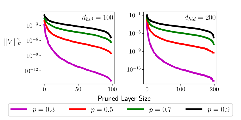
To numerically verify Theorem 5.4, we construct synthetic matrices with different row-compressibility ratios , denoted as . For each , we randomly generate three unique entries within (i.e., ) and present average performance across them all. We prune a randomly-initialized from size to sizes for . (i.e., each setting of is a separate experiment) using .999We find that the active set of neurons selected by i-SpaSP becomes stable (i.e., few neurons are modified) after iterations or less in all synthetic experiments.. We test , and the same matrix is used for experiments with equal hidden dimension; see Appendix A.1 for more details.
Results are displayed in Figure 2, where is shown to decay polynomially with respect to the number of neurons within the pruned network . Furthermore, as predicted by Theorem 5.4, the decay rate of increases as decreases, revealing that higher levels of sparsity within the dense network’s hidden representations improve pruning performance and speed with respect to . This trend holds for all hidden dimensions that were considered.
6.2 Two-Layer Networks
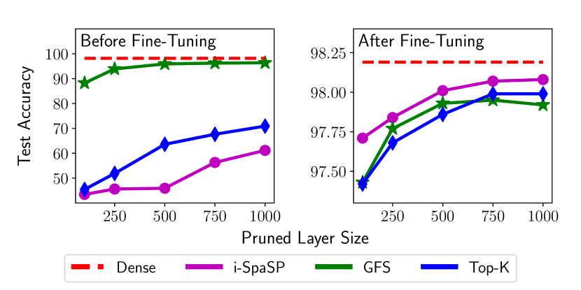
We perform pruning experiments with two-layer networks on MNIST (Deng, 2012). All MNIST images are flattened and no data augmentation is used. The dense network has hidden neurons and is pre-trained before pruning. We prune the dense network using i-SpaSP, GFS, and Top-K, which we use as a naive greedy selection baseline.101010Top-k selects neurons with the largest-magnitude hidden representations in a mini-batch of data. It is a naive baseline for greedy selection that is not used in previous work to the best of our knowledge. After pruning, the network is fine-tuned using stochastic gradient descent (SGD) with momentum. Performance is reported as an average across three separate trails; see Appendix A.2 for more details.
As shown in Figure 3-right, i-SpaSP outperforms other pruning methodologies after fine-tuning in all experimental settings. Networks obtained with GFS perform well without fine-tuning (i.e., Figure 3-left) because neurons are selected to minimize loss during the pruning process. Because i-SpaSP selects neurons based upon the importance criteria described in Section 4, the pruning process does not directly minimize training loss, thus leading to poorer performance prior to fine-tuning (i.e., Top-K exhibits similar behavior). Nonetheless, i-SpaSP, in addition to improving upon the pruning efficiency of GFS, discovers a set of neurons that more closely recovers dense network output, as revealed by its superior performance after fine-tuning.
6.3 Deep Convolutional Networks
We perform structured filter pruning of ResNet34 (He et al., 2015b) and MobileNetV2 (Sandler et al., 2018) with i-SpaSP on ImageNet (ILSVRC 2012). Beginning with public, pre-trained models (Paszke et al., 2017), we use i-SpaSP to prune chosen convolutional blocks within each network, then fine-tune the pruned model using SGD with momentum. After pruning each block, we perform a small amount of fine-tuning; see Appendix A.3 for more details. Numerous heuristic and greedy selection-based algorithms are adopted as baselines; see Table 1.
| Pruning Method | Top-1 Acc. | FLOPS | |
|---|---|---|---|
| ResNet34 | Full Model He et al. (2015b) | 73.4 | 3.68G |
| Filter Pruning Li et al. (2016) | 72.1 | 2.79G | |
| Rethinking Pruning Liu et al. (2018) | 72.0 | 2.79G | |
| More is Less Dong et al. (2017) | 73.0 | 2.75G | |
| i-SpaSP | 73.5 | 2.69G | |
| GFS Ye et al. (2020) | 73.5 | 2.64G | |
| Multi-Layer GFS Ye et al. (2020) | 73.5 | 2.20G | |
| SFP He et al. (2018a) | 71.8 | 2.17G | |
| FPGM He et al. (2019) | 72.5 | 2.16G | |
| i-SpaSP | 72.5 | 2.13G | |
| GFS Ye et al. (2020) | 72.9 | 2.07G | |
| Multi-Layer GFS Ye et al. (2020) | 73.3 | 1.90G | |
| MobileNetV2 | Full Model Sandler et al. (2018) | 72.0 | 314M |
| i-SpaSP | 71.6 | 260M | |
| GFS Ye et al. (2020) | 71.9 | 258M | |
| Multi-Layer GFS Ye et al. (2020) | 72.2 | 245M | |
| i-SpaSP | 71.3 | 242M | |
| LEGR Chin et al. (2019) | 71.4 | 224M | |
| Uniform | 70.0 | 220M | |
| AMC He et al. (2018b) | 70.8 | 220M | |
| i-SpaSP | 70.7 | 220M | |
| GFS Ye et al. (2020) | 71.6 | 220M | |
| Multi-Layer GFS Ye et al. (2020) | 71.7 | 218M | |
| Meta Pruning Liu et al. (2019) | 71.2 | 217M |
ResNet34. We prune ResNet34 to 2.69 and 2.13 GFlops with i-SpaSP. As shown in Table 1, i-SpaSP yields comparable performance to GFS variants at similar FLOP levels; e.g., i-SpaSP matches 75.5% test accuracy of GFS with the 2.69 GFlop model and performs within 1% of GFS variants for the 2.13 GFlop model. However, the multi-layer variant of GFS (Ye et al., 2020) does discover sub-networks with fewer FLOPS and similar performance in both cases. i-SpaSP improves upon or matches the performance of all heuristic methods at similar FLOP levels.
MobileNetV2. We prune MobileNetV2 to 260, 242, and 220 MFlops with i-SpaSP. In all cases, sub-networks discovered with i-SpaSP achieve performance within 1% of those obtained via both GFS variants and heuristic methods. Although MobileNetV2 performance is relatively lower in comparison to ResNet34, i-SpaSP is still capable of pruning the more difficult network to various different FLOP levels and performs comparably to baselines in all cases.
Discussion. Within Table 1, the performance of i-SpaSP is never more than 1% below that of a similar-FLOP model obtained with a baseline pruning methodology, including both greedy selection and heuristic-based methods. As such, similar to GFS, i-SpaSP can be seen as a theoretically-grounded pruning methodology that is practically useful, even in large-scale experiments. Such pruning methodologies that are both theoretically and practically relevant are few. In comparison to GFS variants, i-SpaSP significantly improves pruning efficiency; see Section 4.2. Thus, i-SpaSP can be seen as a viable alternative to GFS—both theoretically and practically—that may be preferable when runtime is a major concern.
6.4 Transformer Networks
| Method | Pruning Ratio | Top-1 Acc. |
|---|---|---|
| Full Model | - | 71.02 |
| Uniform | 25% | 62.73 |
| 40% | 66.43 | |
| Michel et al. (2019) | 25% | 62.97 |
| 40% | 67.31 | |
| i-SpaSP | 25% | 63.70 |
| 40% | 68.11 |
We perform structured pruning of attention heads using the mBERT model (Devlin et al., 2018) on the XNLI dataset (Conneau et al., 2018), which contains textual entailment annotations across 15 different languages. We begin with a pre-trained mBERT model and fine-tune it on XNLI prior to pruning. Then, structured pruning is performed on the attention heads of each layer using i-SpaSP, uniform pruning (i.e., randomly removing a fixed ratio of attention heads), and a sensitivity-based masking approach (Michel et al., 2019) (i.e., a state-of-the-art heuristic approach for structured attention head pruning for transformers). After pruning models to a fixed ratio of 25% or 40% of original attention heads, we fine-tune the pruned networks and record their performance on the XNLI test set; see Appendix A.4 for further details.
As shown in Table 2, models pruned with i-SpaSP outperform those pruned to the same ratio with either uniform or heuristic pruning methods in all cases. The ability of i-SpaSP to effectively prune transformers demonstrates that the methodology can be applied to the structured pruning of numerous different architectures without significant implementation changes (i.e., using the automatic differentiation approach described in Section 4.1). Furthermore, i-SpaSP even outperforms a state-of-the-art heuristic approach for the structured pruning of transformer attention heads, thus again highlighting the strong empirical performance of i-SpaSP in comparison to heuristic pruning methods that lack theoretical guarantees.
7 Conclusion
We propose i-SpaSP, a pruning methodology for neural networks inspired by sparse signal recovery. Our methodology comes with theoretical guarantees that indicate, for both two and multi-layer networks, the quality of a pruned network decays polynomially with respect to its size. We connect this theoretical analysis to properties of the dense network, showing that pruning performance improves as the dense network’s hidden representations become more sparse. Practically, i-SpaSP performs comparably to numerous baseline pruning methodologies in large-scale experiments and drastically improves upon the computationally efficiency of the most common provable pruning methodologies. As such, i-SpaSP is a practical, provable, and efficient algorithm that we hope will enable a better understanding of neural network pruning both in theory and practice. In future work, we wish to extend i-SpaSP to cover cases in which network pruning and training are combined into a single process, such as utilizing regularization-based approaches to induce sparsity during pre-training or updating network weights to improve sub-network performance as pruning occurs.
Compute resources used for this work were provided by Alegion Inc. This work is supported by NSF FET:Small no. 1907936, NSF MLWiNS CNS no. 2003137 (in collaboration with Intel), NSF CMMI no. 2037545, NSF CAREER award no. 2145629, and Rice InterDisciplinary Excellence Award (IDEA).
References
- Abadi et al. (2015) Martín Abadi, Ashish Agarwal, Paul Barham, Eugene Brevdo, Zhifeng Chen, Craig Citro, Greg S. Corrado, Andy Davis, Jeffrey Dean, Matthieu Devin, Sanjay Ghemawat, Ian Goodfellow, Andrew Harp, Geoffrey Irving, Michael Isard, Yangqing Jia, Rafal Jozefowicz, Lukasz Kaiser, Manjunath Kudlur, Josh Levenberg, Dan Mané, Rajat Monga, Sherry Moore, Derek Murray, Chris Olah, Mike Schuster, Jonathon Shlens, Benoit Steiner, Ilya Sutskever, Kunal Talwar, Paul Tucker, Vincent Vanhoucke, Vijay Vasudevan, Fernanda Viégas, Oriol Vinyals, Pete Warden, Martin Wattenberg, Martin Wicke, Yuan Yu, and Xiaoqiang Zheng. TensorFlow: Large-scale machine learning on heterogeneous systems, 2015.
- Bach (2014) Francis Bach. Breaking the Curse of Dimensionality with Convex Neural Networks. arXiv e-prints, art. arXiv:1412.8690, December 2014.
- Bah and Tanner (2018) Bubacarr Bah and Jared Tanner. On the construction of sparse matrices from expander graphs. Frontiers in Applied Mathematics and Statistics, 4:39, 2018.
- Baykal et al. (2018) Cenk Baykal, Lucas Liebenwein, Igor Gilitschenski, Dan Feldman, and Daniela Rus. Data-dependent coresets for compressing neural networks with applications to generalization bounds. arXiv preprint arXiv:1804.05345, 2018.
- Baykal et al. (2019) Cenk Baykal, Lucas Liebenwein, Igor Gilitschenski, Dan Feldman, and Daniela Rus. SiPPing Neural Networks: Sensitivity-informed Provable Pruning of Neural Networks. arXiv e-prints, art. arXiv:1910.05422, October 2019.
- Candes and Tao (2006) Emmanuel J Candes and Terence Tao. Near-optimal signal recovery from random projections: Universal encoding strategies? IEEE transactions on information theory, 52(12):5406–5425, 2006.
- Chen et al. (2020) Xiaohan Chen, Yu Cheng, Shuohang Wang, Zhe Gan, Zhangyang Wang, and Jingjing Liu. EarlyBERT: Efficient BERT Training via Early-bird Lottery Tickets. arXiv e-prints, art. arXiv:2101.00063, December 2020.
- Chin et al. (2019) Ting-Wu Chin, Ruizhou Ding, Cha Zhang, and Diana Marculescu. Legr: Filter pruning via learned global ranking. 2019.
- Conneau et al. (2018) Alexis Conneau, Ruty Rinott, Guillaume Lample, Adina Williams, Samuel R. Bowman, Holger Schwenk, and Veselin Stoyanov. Xnli: Evaluating cross-lingual sentence representations. In Proceedings of the 2018 Conference on Empirical Methods in Natural Language Processing. Association for Computational Linguistics, 2018.
- Deng (2012) Li Deng. The mnist database of handwritten digit images for machine learning research. IEEE Signal Processing Magazine, 29(6):141–142, 2012.
- Devlin et al. (2018) Jacob Devlin, Ming-Wei Chang, Kenton Lee, and Kristina Toutanova. Bert: Pre-training of deep bidirectional transformers for language understanding. arXiv preprint arXiv:1810.04805, 2018.
- Dong et al. (2017) Xuanyi Dong, Junshi Huang, Yi Yang, and Shuicheng Yan. More is less: A more complicated network with less inference complexity. In Proceedings of the IEEE Conference on Computer Vision and Pattern Recognition, pages 5840–5848, 2017.
- Edelman and Wang (2013) Alan Edelman and Yuyang Wang. Random matrix theory and its innovative applications. In Advances in Applied Mathematics, Modeling, and Computational Science, pages 91–116. Springer, 2013.
- Evci et al. (2019) Utku Evci, Trevor Gale, Jacob Menick, Pablo Samuel Castro, and Erich Elsen. Rigging the Lottery: Making All Tickets Winners. arXiv e-prints, art. arXiv:1911.11134, November 2019.
- Evci et al. (2020) Utku Evci, Yani A. Ioannou, Cem Keskin, and Yann Dauphin. Gradient Flow in Sparse Neural Networks and How Lottery Tickets Win. arXiv e-prints, art. arXiv:2010.03533, October 2020.
- Frank et al. (1956) Marguerite Frank, Philip Wolfe, et al. An algorithm for quadratic programming. Naval research logistics quarterly, 3(1-2):95–110, 1956.
- Frankle and Carbin (2018) Jonathan Frankle and Michael Carbin. The Lottery Ticket Hypothesis: Finding Sparse, Trainable Neural Networks. arXiv e-prints, art. arXiv:1803.03635, March 2018.
- Frankle et al. (2019) Jonathan Frankle, Gintare Karolina Dziugaite, Daniel M. Roy, and Michael Carbin. Stabilizing the Lottery Ticket Hypothesis. arXiv e-prints, art. arXiv:1903.01611, March 2019.
- Han et al. (2015) Song Han, Huizi Mao, and William J. Dally. Deep Compression: Compressing Deep Neural Networks with Pruning, Trained Quantization and Huffman Coding. arXiv e-prints, art. arXiv:1510.00149, October 2015.
- Han et al. (2015a) Song Han, Huizi Mao, and William J Dally. Deep compression: Compressing deep neural networks with pruning, trained quantization and huffman coding. arXiv preprint arXiv:1510.00149, 2015a.
- Han et al. (2015b) Song Han, Jeff Pool, John Tran, and William J Dally. Learning both weights and connections for efficient neural networks. arXiv preprint arXiv:1506.02626, 2015b.
- Han et al. (2016) Song Han, Xingyu Liu, Huizi Mao, Jing Pu, Ardavan Pedram, Mark A. Horowitz, and William J. Dally. EIE: Efficient Inference Engine on Compressed Deep Neural Network. arXiv e-prints, art. arXiv:1602.01528, February 2016.
- He et al. (2015a) Kaiming He, Xiangyu Zhang, Shaoqing Ren, and Jian Sun. Delving Deep into Rectifiers: Surpassing Human-Level Performance on ImageNet Classification. arXiv e-prints, art. arXiv:1502.01852, February 2015a.
- He et al. (2015b) Kaiming He, Xiangyu Zhang, Shaoqing Ren, and Jian Sun. Deep Residual Learning for Image Recognition. arXiv e-prints, art. arXiv:1512.03385, December 2015b.
- He et al. (2018a) Yang He, Guoliang Kang, Xuanyi Dong, Yanwei Fu, and Yi Yang. Soft filter pruning for accelerating deep convolutional neural networks. arXiv preprint arXiv:1808.06866, 2018a.
- He et al. (2019) Yang He, Ping Liu, Ziwei Wang, Zhilan Hu, and Yi Yang. Filter pruning via geometric median for deep convolutional neural networks acceleration. In Proceedings of the IEEE/CVF Conference on Computer Vision and Pattern Recognition, pages 4340–4349, 2019.
- He et al. (2017) Yihui He, Xiangyu Zhang, and Jian Sun. Channel Pruning for Accelerating Very Deep Neural Networks. arXiv e-prints, art. arXiv:1707.06168, July 2017.
- He et al. (2018b) Yihui He, Ji Lin, Zhijian Liu, Hanrui Wang, Li-Jia Li, and Song Han. Amc: Automl for model compression and acceleration on mobile devices. In Proceedings of the European conference on computer vision (ECCV), pages 784–800, 2018b.
- Huang and Wang (2018) Zehao Huang and Naiyan Wang. Data-driven sparse structure selection for deep neural networks. In Proceedings of the European conference on computer vision (ECCV), pages 304–320, 2018.
- Khanna and Kyrillidis (2018) Rajiv Khanna and Anastasios Kyrillidis. Iht dies hard: Provable accelerated iterative hard thresholding. In International Conference on Artificial Intelligence and Statistics, pages 188–198. PMLR, 2018.
- Li et al. (2016) Hao Li, Asim Kadav, Igor Durdanovic, Hanan Samet, and Hans Peter Graf. Pruning Filters for Efficient ConvNets. arXiv e-prints, art. arXiv:1608.08710, August 2016.
- Liebenwein et al. (2019) Lucas Liebenwein, Cenk Baykal, Harry Lang, Dan Feldman, and Daniela Rus. Provable filter pruning for efficient neural networks. arXiv preprint arXiv:1911.07412, 2019.
- Liu et al. (2019) Zechun Liu, Haoyuan Mu, Xiangyu Zhang, Zichao Guo, Xin Yang, Kwang-Ting Cheng, and Jian Sun. Metapruning: Meta learning for automatic neural network channel pruning. In Proceedings of the IEEE/CVF International Conference on Computer Vision, pages 3296–3305, 2019.
- Liu et al. (2017) Zhuang Liu, Jianguo Li, Zhiqiang Shen, Gao Huang, Shoumeng Yan, and Changshui Zhang. Learning Efficient Convolutional Networks through Network Slimming. arXiv e-prints, art. arXiv:1708.06519, August 2017.
- Liu et al. (2018) Zhuang Liu, Mingjie Sun, Tinghui Zhou, Gao Huang, and Trevor Darrell. Rethinking the Value of Network Pruning. arXiv e-prints, art. arXiv:1810.05270, October 2018.
- Luo et al. (2017) Jian-Hao Luo, Jianxin Wu, and Weiyao Lin. ThiNet: A Filter Level Pruning Method for Deep Neural Network Compression. arXiv e-prints, art. arXiv:1707.06342, July 2017.
- Malach et al. (2020) Eran Malach, Gilad Yehudai, Shai Shalev-Shwartz, and Ohad Shamir. Proving the Lottery Ticket Hypothesis: Pruning is All You Need. arXiv e-prints, art. arXiv:2002.00585, February 2020.
- Michel et al. (2019) Paul Michel, Omer Levy, and Graham Neubig. Are sixteen heads really better than one? Advances in neural information processing systems, 32, 2019.
- Molchanov et al. (2016) Pavlo Molchanov, Stephen Tyree, Tero Karras, Timo Aila, and Jan Kautz. Pruning convolutional neural networks for resource efficient inference. arXiv preprint arXiv:1611.06440, 2016.
- Mussay et al. (2019) Ben Mussay, Margarita Osadchy, Vladimir Braverman, Samson Zhou, and Dan Feldman. Data-independent neural pruning via coresets. arXiv preprint arXiv:1907.04018, 2019.
- Needell and Tropp (2009) Deanna Needell and Joel A Tropp. Cosamp: Iterative signal recovery from incomplete and inaccurate samples. Applied and computational harmonic analysis, 26(3):301–321, 2009.
- Nemhauser et al. (1978) George L Nemhauser, Laurence A Wolsey, and Marshall L Fisher. An analysis of approximations for maximizing submodular set functions—i. Mathematical programming, 14(1):265–294, 1978.
- Orseau et al. (2020) Laurent Orseau, Marcus Hutter, and Omar Rivasplata. Logarithmic Pruning is All You Need. arXiv e-prints, art. arXiv:2006.12156, June 2020.
- Paszke et al. (2017) Adam Paszke, Sam Gross, Soumith Chintala, Gregory Chanan, Edward Yang, Zachary DeVito, Zeming Lin, Alban Desmaison, Luca Antiga, and Adam Lerer. Automatic differentiation in pytorch. 2017.
- Pensia et al. (2020) Ankit Pensia, Shashank Rajput, Alliot Nagle, Harit Vishwakarma, and Dimitris Papailiopoulos. Optimal lottery tickets via subsetsum: Logarithmic over-parameterization is sufficient. arXiv preprint arXiv:2006.07990, 2020.
- Pokutta et al. (2020) Sebastian Pokutta, Christoph Spiegel, and Max Zimmer. Deep Neural Network Training with Frank-Wolfe. arXiv e-prints, art. arXiv:2010.07243, October 2020.
- Ramanujan et al. (2019) Vivek Ramanujan, Mitchell Wortsman, Aniruddha Kembhavi, Ali Farhadi, and Mohammad Rastegari. What’s Hidden in a Randomly Weighted Neural Network? arXiv e-prints, art. arXiv:1911.13299, November 2019.
- Sandler et al. (2018) Mark Sandler, Andrew Howard, Menglong Zhu, Andrey Zhmoginov, and Liang-Chieh Chen. Mobilenetv2: Inverted residuals and linear bottlenecks. In Proceedings of the IEEE conference on computer vision and pattern recognition, pages 4510–4520, 2018.
- Suau et al. (2020) Xavier Suau, Nicholas Apostoloff, et al. Filter distillation for network compression. In 2020 IEEE Winter Conference on Applications of Computer Vision (WACV), pages 3129–3138. IEEE, 2020.
- Wang et al. (2020) Chaoqi Wang, Guodong Zhang, and Roger Grosse. Picking Winning Tickets Before Training by Preserving Gradient Flow. arXiv e-prints, art. arXiv:2002.07376, February 2020.
- Wolfe et al. (2021) Cameron R Wolfe, Qihan Wang, Junhyung Lyle Kim, and Anastasios Kyrillidis. Provably efficient lottery ticket discovery. arXiv preprint arXiv:2108.00259, 2021.
- Ye (2021) Mao Ye. Network-pruning-greedy-forward-selection. https://github.com/lushleaf/Network-Pruning-Greedy-Forward-Selection, 2021.
- Ye et al. (2020) Mao Ye, Chengyue Gong, Lizhen Nie, Denny Zhou, Adam Klivans, and Qiang Liu. Good subnetworks provably exist: Pruning via greedy forward selection. In International Conference on Machine Learning, pages 10820–10830. PMLR, 2020.
- Ye et al. (2020) Mao Ye, Lemeng Wu, and Qiang Liu. Greedy Optimization Provably Wins the Lottery: Logarithmic Number of Winning Tickets is Enough. arXiv e-prints, art. arXiv:2010.15969, October 2020.
- You et al. (2019) Haoran You, Chaojian Li, Pengfei Xu, Yonggan Fu, Yue Wang, Xiaohan Chen, Richard G Baraniuk, Zhangyang Wang, and Yingyan Lin. Drawing early-bird tickets: Towards more efficient training of deep networks. arXiv preprint arXiv:1909.11957, 2019.
- Yu et al. (2017) Ruichi Yu, Ang Li, Chun-Fu Chen, Jui-Hsin Lai, Vlad I. Morariu, Xintong Han, Mingfei Gao, Ching-Yung Lin, and Larry S. Davis. NISP: Pruning Networks using Neuron Importance Score Propagation. arXiv e-prints, art. arXiv:1711.05908, November 2017.
- Zhang et al. (2021) Shuai Zhang, Meng Wang, Sijia Liu, Pin-Yu Chen, and Jinjun Xiong. Why lottery ticket wins? a theoretical perspective of sample complexity on pruned neural networks. arXiv preprint arXiv:2110.05667, 2021.
- Zhuang et al. (2018) Zhuangwei Zhuang, Mingkui Tan, Bohan Zhuang, Jing Liu, Yong Guo, Qingyao Wu, Junzhou Huang, and Jinhui Zhu. Discrimination-aware Channel Pruning for Deep Neural Networks. arXiv e-prints, art. arXiv:1810.11809, October 2018.
Appendix A Experimental Details
A.1 Synthetic Experiments
Here, we present the details for generating the synthetic data used for pruning experiments with i-SpaSP on two-layer neural networks presented in Section 6.1. It should be noted that the synthetic data generated within this set of experiments does not correspond to the input data matrix described in Section 2. Rather, the synthetic data that is generated corresponds to the hidden representation of a two-layer neural network, constructed as for some input . Within these experiments, we generate hidden representations instead of raw input because the row-compressibility ratio considered within Theorem 5.4 is with respect to the neural network’s hidden representations (i.e., not with respect to the input).
Consider the -th synthetic hidden representation matrix , and assume this matrix has a desired row-compressibility ratio . For all experiments, we set (i.e., the size of the dataset) to be 100. Recall that all entries within must be non-negative due to the ReLU activation present within (1). For each row of the matrix, the synthetic hidden representation is generated by computing the upper bound on the sum of the values within this -th row as and randomly sampling non-negative values that, when summed together, do not exceed the upper bound.111111In practice, this is implemented by keeping a running sum and continually sampling numbers randomly within a range that does not exceed the upper bound. Here, is a scalar constant as described in Section 2, which we set to . After this process has been completed for each row, the rows of are randomly shuffled so as to avoid rows being in sorted, magnitude order.
Within the experiments presented in Section 6.1, we generate three random matrices, following the process described above, for each combination of and . Then, the average pruning results across each of these three matrices is reported for each experimental setting. Experiments were also replicated with different settings of , but the results observed were quite similar. Further, the matrix used within the synthetic experiments of Section 6.1 was generated using standard Kaiming initialization (He et al., 2015a), which is supported in deep learning packages like PyTorch (Paszke et al., 2017).
A.2 Two-Layer Networks
Within this section, we provide all relevant experimental details for pruning experiments with two-layer networks presented in Section 6.2.
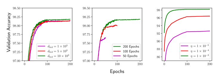
Baseline Network. We begin by describing the baseline two-layer network that was used within pruning experiments on MNIST, as well as relevant details for pre-training the network prior to pruning. The network used within experiments in Section A.2 exactly matches the formulation in (1), and MNIST images are flattened—forming a 784-dimensional input vector—prior to being passed as input to the network. The network is first pre-trained on the MNIST dataset such that it has fully converged before being used in pruning experiments. During pre-training, we optimize the network with stochastic gradient descent (SGD) using a batch size of 128 and employ a learning rate step schedule that decays the learning rate after completing 50% and 75% of total epochs. For all network and pre-training hyperparameters, we identify optimal settings by dividing the MNIST training set randomly (i.e., a random, 80-20 split) into training and validation sets. Then, performance is measured over the validation set using three separate trials and averaged to identify proper hyperparameter settings.
We find that weight decay and momentum settings do not significantly impact network performance. Thus, we use no weight decay during pre-training and set momentum to 0.9. The results of other hyperparameter tuning experiments are provided in Figure 4. We test different hidden dimensions of the two-layer network , finding that validation performance reaches a plateau when . We also test numerous possible learning rates and pre-training epochs. Within these experiments, it is determined that a learning rate of with 200 epochs of pre-training acheives the best performance on the validation set; as shown in the right and middle subplots of Figure 4. Thus, the dense networks used for experiments within Section 6.2 has a hidden dimension of and is pre-trained for 200 epochs using a learning rate of prior to pruning being performed.
Network Pruning. The two-layer network described above is pruned using several greedy selection strategies, including i-SpaSP, GFS, and Top-K. Each of these pruning strategies selects a subset of neurons within the dense network’s hidden layer based on a mini-batch of data from the training set. Within all experiments, we adopt a batch size of 512 for pruning.
For i-SpaSP, the pruning procedure follows the exact steps outlined in Algorithm 1. Within each iteration of Algorithm 1, a new mini-batch of data is sampled to compute neuron importance. We use a fixed number of iterations as the stopping criterion for i-SpaSP. In particular, we terminate the algorithm and return the pruned model after 20 iterations, as the active set of neurons is consistently stable at this point.
An in-depth description of GFS is provided in (Ye et al., 2020). For two-layer networks, GFS is implemented by, at each iteration, sampling a new mini-batch of data and finding the neuron that, when included in the (initially empty) active set, yields the largest decrease in loss over the mini-batch. This process is repeated until the desired size of the pruned network has been reached—i.e., each iteration adds a single neuron to the pruned network and the size of the pruned network is used as a stopping criterion. Top-K is a naive, baseline method for greedy selection, which operates by computing hidden representations across the mini-batch and selecting the neurons with the largest-magnitude hidden activations (i.e., based on summing hidden representation magnitudes across the mini-batch). Top-K performs the entire pruning process in one step using a single mini-batch.
A.3 Deep Convolutional Networks
Within this section, we provide relevant details to the large-scale CNN experiments on ImageNet (ILSVRC2012) presented in Section 6.3.
Pruning Deep Networks. As described in Section 4.1, i-SpaSP is extended to deep networks by greedily pruning each layer of the network from beginning to end. We prune filters within each block of the network independently, where a block either consists of two convolution operations separated by batch normalization and ReLU (i.e., BasicBlock for ResNet34) or a depth-wise, separable convolution with a linear bottleneck (i.e., InvertedResidualBlock for MobileNetV2). We maintain the input and output channel resolution of each block—choosing instead to reduce each block’s intermediate channel dimension—by performing pruning as follows:
-
•
BasicBlock: We obtain the output of the first convolution (i.e., after batch normalization and ReLU) and perform pruning based on the forward pass of the second convolution, thus eliminating filters from the output of the first convolution and, in turn, the input of the second convolution.
-
•
InvertedResidualBlock: We obtain the output of the first point-wise and depth-wise convolutions (i.e., after normalization and ReLU) and prune the filters of this representation based on the forward pass of the last point-wise linear convolution, thus removing filters from the output of the first point-wise convolution and, in turn, within the depth-wise convolution operation.
Thus, each convolutional block is separated into two components. Input data is passed through the first component to generate a hidden representation, then i-SpaSP performs pruning using forward and backward passes of the second component as in Algorithm 1. Intuitively, one can view the two components of each block as the two neural network layers in (1). Due to implementation with automatic differentiation, pruning convolutional layers is nearly identical to pruning two-layer network as described in Section 4.1, the only difference being the need to sum over both batch and spatial dimensions in computing importance.
Pruning Ratios. As mentioned within Section 6.3, some blocks within each network are more sensitive to pruning than others. Thus, pruning all layers to a uniform ratio typically does not perform well. Within ResNet34, four groups of convolutional blocks exist, where each group contains a sequence of convolutional blocks with the same channel dimension. Following the recommendations of Li et al. (2016), we avoid pruning the fourth group of convolutional blocks, any strided blocks, or the last block in any group. The 2.69 GFlop model in Table 1 uses a uniform ratio of 40% for all three groups (i.e., 60% of filters are eliminated from each block). For the 2.13 GFlop model, the first group is pruned to a ratio of 20%, while the second and third groups are pruned to a ratio of 30%.
Within MobileNetV2, we simply avoid pruning network blocks that are either strided or have different input and output channel dimensions, leaving the following blocks to be pruned: 3, 5, 6, 8, 9, 10, 12, 13, 15, 16. We find that blocks 3, 5, 8, 15, and 16 are especially sensitive to pruning (i.e., pruning these layers causes noticeable performance degradation), so we avoid aggressive pruning upon these blocks. The 260 MFlop model is generated by pruning only blocks 6, 9, 10, 12, and 13 to a ratio of 40%. For the 242 MFlop and 220 MFlop models, we prune sensitive (i.e., blocks 3, 4, 8, 15, and 16) and not sensitive (i.e., blocks 6, 9, 10, 12, and 13) blocks with ratios of 40%/80% and 30%/70%, respectively. For the 220 MFlop model, we also prune blocks 2, 11, and 17 to a ratio of 90% to further decrease the FLOP count.
Pruning Hyperparameters. Pruning of each layer is performed with a batch of 1280 data examples for both ResNet34 and MobileNetV2 architectures. This batch of data can be separated into multiple mini-batches (e.g., of size 256) during pruning. Such an approach allows the computation of i-SpaSP to be performed on a GPU (i.e., all of the data examaples cannot simultaneously fit within memory of a typical GPU), but this modification does not change the runtime of behavior of i-SpaSP. Furthermore, 20 total i-SpaSP iterations are performed in pruning each layer. We find that adding more data or pruning iterations beyond these settings does not provide any benefit to i-SpaSP performance.
Fine-tuning Details. For fine-tuning, we perform 90 epochs of fine-tuning using SGD with momentum and employ a cosine learning rate decay schedule over the entire fine-tuning process beginning with a learning rate of 0.01. For fine-tuning between the pruning of layers (i.e., a small amount of fine-tuning is performed after each layer is pruned), we simply adopt the same fine-tuning setup with a fixed learning rate of 0.01 and fine-tuning continues for one epoch. Our learning rate setup for fine-tuning matches that of (Ye et al., 2020, 2020), but we choose to perform fewer epochs of fine-tuning, as we find network performance does not improve much after 90 epochs. In all cases, we adopt standard augmentation procedures for the ImageNet dataset during fine-tuning (i.e., normalizing the data and performing random crops and flips).
A.4 Transformer Networks
Within this section, we provide all relevant experimental details for pruning experiments with two-layer networks presenting in Section 6.4.
Baseline Network. We begin by describing the baseline network used within the structured attention head pruning experiments. The network architecture used in all experiments is the multi-lingual BERT (mBERT) model (Devlin et al., 2018). More specifically, we adopt the BERT-base-cased variant of the architecture, which is pre-trained on a corpus of over 100 different languages. Beginning with this pre-trained network architecture, we fine-tune the BERT model on the XNLI dataset for two epochs with the AdamW optimizer and a learning rate of that is decayed linearly throughout the training process. After the fine-tuning process, this model achieves an accuracy of 71.02% on the XNLI test set.
Network Pruning. For all pruning experiments, we adopt a structured pruning approach that selectively removes entire attention heads from network layers. We adopt two different pruning ratios: 25% and 40%.121212Here, the pruning ratio refers to the number of attention heads remaining after pruning. For example, a 12-head layer pruned at a ratio of 25% would have three remaining heads after pruning completes. These ratios correspond to three and five attention heads (i.e., each layer of mBERT originally has 12 attention heads) being retained within each layer of the network.
We compare the performance of i-SpaSP to a uniform pruning approach (i.e., randomly select attention heads to prune within each layer) and a sensitivity-based, global pruning approach that was previously proposed for structured pruning of attention heads (Michel et al., 2019). For i-SpaSP and uniform pruning, one layer is pruned at a time, starting from the first layer of the network and ending at the final layer. For the sensitivity-based pruning technique, the pruning process is global and all layers are pruned simultaneously. After pruning has been completed, networks are fine-tuned for 0.5 epochs using the AdamW optimizer with a learning rate of that is decayed linearly throughout the fine-tuning process. For i-SpaSP and the sensitivity-based pruning approach, we adopt the same setting as previous experiments (i.e., see Section 6.3) and utilize a subset of 1280 training data examples for pruning. Additionally, i-SpaSP performs 20 total iterations for the pruning of each layer, which again reflects the settings used within previous experiments.
Appendix B Main Proofs
B.1 Properties of
Prior to providing any proofs of our theoretical results, we show a few properties of the function defined over matrices that will become useful in deriving later results. Given , and is defined as follows:
In words, sums all columns within an arbitraty matrix to produce a single column vector. We now provide a few useful properties of .
Lemma B.1.
Consider two arbitrary matrices and . The following properties of must be true.
Proof B.2.
Given the matrices and , we can arrive at the first property as follows:
Furthermore, the second property can be shown as follows:
B.2 Proof of Lemma 5.1
Proof B.3.
Consider an arbitrary iteration of Algorithm 1. We define the active neurons within the pruned network entering this iteration as . The notation will be used to refer to the active neurons in the pruned model after the completion of the iteration. Similarly, we will use the notation to refer to other constructions after the iteration completes (e.g., becomes , becomes , etc.)
We begin by defining and expanding the definitions of the matrices , , , and considering the substitution of ;
Now, observe the following about .
where we denote . It should be noted that is simply the matrix with all the -th rows set to zero where . Invoking Lemma B.1 in combination with the above expression, we can show the following.
Based on the definition of , must be -row-sparse. This is because is -row-sparse and . Thus, the number of non-zero rows within must be less than or equal to (i.e., the rows that are not subtracted out of by ). Denote , where . From the definition of in Algorithm 1, we have the following properties of :
where follows by removing indices within . From here, we can upper bound the value of as follows.
where follows from the triangle inequality, holds from Corrolary 3.3 on RIP properties of in (Needell and Tropp, 2009) because , holds from Proposition 3.1 on RIP properties of in (Needell and Tropp, 2009) because , and holds from Proposition 3.5 on RIP properties of in (Needell and Tropp, 2009). Now, we can also lower bound the value of as follows:
where follows from the triangle inequality. follows from Proposition 3.1 in (Needell and Tropp, 2009) and follows from Corollary 3.3 and Proposition 3.1 in (Needell and Tropp, 2009) because . Finally, follows from Proposition 3.5 within (Needell and Tropp, 2009). By noting that and combining the lower and upper bounds above, we derive the following:
| (4) |
From here, we can show the following:
| (5) |
where follows from the fact that , follows from the fact that , and follows from the triangle inequality. Then, as a final step, we make the following observation, where we leverage notation from Algorithm 1:
| (6) |
where follow from the triangle inequality and follows from the fact that is the best -sparse approximation to (i.e., is a worse -sparse approximation with respect to the norm). Now, noticing that , we can aggregate all of this information as follows:
where holds because , holds from (6), holds from (5), and hold from (4). By simply moving the term to the other side of the inequality, we get the following:
From here, we recover from as follows:
where holds from the triangle inequality. Combining this with the final inequality derived above, we arrive at the following recursion for error between pruned and dense model hidden layers over iterations of Algorithm 1:
We now adopt an identical numerical assumption as (Needell and Tropp, 2009) and assume that has restricted isometry constant . Then, noting that per Corollary 3.4 in (Needell and Tropp, 2009), we substitute the restricted isometry constants into the above recursion to yield the following expression:
If we invoke Lemma B.1, unroll the above recursion over iterations of Algorithm 1, notice it is always true that and , and draw upon the property of and vector norms that we arrive at the desired result:
B.3 Proof of Theorem 5.2
Proof B.4.
Consider an arbitrary iteration of Algorithm 1 with a set of active neurons within the pruned model denoted by . The matrix contains the residual between the dense and pruned model output over the entire dataset, as formalized below:
Consider the squared Frobenius norm of the matrix . We can show the following:
where follows from the Cauchy-Schwarz inequality and follows from the fact that all entries of are non-negative. From here, we simply invoke Lemma 5.1 to arrive at the desired result.
B.4 Proof of Lemma 5.3
Proof B.5.
Assume that we choose the -row-sparse matrix within as follows
The norm used within the above expression is arbitrary, as we simply care to select indices such that contains the largest-magnitude components of . Such a property will be true for any norm selection within the above equation, as they all ensure is the best possible -sparse approximation of . From here, we have that , which yields the following:
where holds from Lemma B.1 and is a bound on the norm of the best-possible -sparse approximation of a -compressible vector; see Section 2.6 in (Needell and Tropp, 2009).
B.5 Proof of Theorem 5.6
Here, we generalize our theoretical results beyond single-hidden-layer networks to arbitrary depth networks. For this section, we define the forward pass in a -hidden-layer network via the following recursion:
where denotes the nonlinear ReLU activation applied at each layer and we have weight matrices and hidden representations for each of the layers within the network. Here, denotes the network output and . It should be noted that no ReLU activation is applied at the final network output (i.e., ). We denote the pre-activation values each hidden representation as .
Proof B.6.
We denote the active set of neurons after iterations at each layer as . The dense network output is given by , and we compute the residual between pruned and dense networks at layer as . We further denote as shorthand for intermediate, pre-activation outputs of the pruned network. For simplicity, we assume all hidden layers of the multi-layer network have the same number of hidden neurons and are pruned to a size , such that . Consider the final output representation of an -hidden-layer network . We will now bound , revealing that a recursion can be derived over the layers of the network to upper bound the norm of the final layer’s residual between pruned and dense networks.
Following previous proofs, we decompose the hidden representation at each layer prior to the output layer as , where is an -row-sparse matrix and and are both arbitrary-valued matrices. denotes the same arbitrarily-valued matrix from the previous formulation and captures all error introduced by pruning layers prior to within the network. and can also be combined into a single matrix as . Now, we consider the value of :
| (7) |
where holds from Theorem 5.2, holds from the triangle inequality, and holds by eliminating all terms that approach zero with enough pruning iterations . Now, notice that characterizes the error induced by pruning within the previous layer of the network, following the ReLU activation. Thus, our expression for the error induced by pruning on network output is now expressed with respect to the pruning error of the previous layer, revealing that a recursion can be derived for pruning error over the entire multi-layer network. We now expand the expression for (i.e., we use arbitrary layer to enable a recursion over layers to be derived).
where holds because simply characterizes the difference between pruned and dense network hidden representations, holds due to properties of the ReLU function, hold by expanding the expression as a sum and replacing the ReLU operation with absolute value, holds due to the Cauchy Schwarz inequality, holds due to properties of norms, holds due to Lemma 5.1, and holds due to the triangle inequality. As can be seen within the above expression, the value of can be expressed with respect to . Now, by beginning with (7) and unrolling the equation above over all layers of the network, we obtain the following
Now, assume that is -row-compressible with factor for . Then, defining and , we invoke Lemma 5.3 to arrive at the desired result
where is factored out because it has no asymptotic impact on the expression.