Sampling rate-corrected analysis of irregularly sampled time series

Abstract

The analysis of irregularly sampled time series remains a challenging task requiring methods that account for continuous and abrupt changes of sampling resolution without introducing additional biases. The edit–distance is an effective metric to quantitatively compare time series segments of unequal length by computing the cost of transforming one segment into the other. We show that transformation costs generally exhibit a non-trivial relationship with local sampling rate. If the sampling resolution undergoes strong variations, this effect impedes unbiased comparison between different time episodes. We study the impact of this effect on recurrence quantification analysis, a framework that is well-suited for identifying regime shifts in nonlinear time series. A constrained randomization approach is put forward to correct for the biased recurrence quantification measures. This strategy involves the generation of a novel type of time series and time axis surrogates which we call sampling rate constrained (SRC) surrogates. We demonstrate the effectiveness of the proposed approach with a synthetic example and an irregularly sampled speleothem proxy record from Niue island in the central tropical Pacific. Application of the proposed correction scheme identifies a spurious transition that is solely imposed by an abrupt shift in sampling rate and uncovers periods of reduced seasonal rainfall predictability associated with enhanced ENSO and tropical cyclone activity.

I Introduction

The analysis of time series from complex systems calls for numerical methods that capture the most relevant features in the observed variability. At the same time, the impact of various frequently encountered data-related intricacies such as low signal-to-noise ratio, nonstationarity, and limited time series length must be accounted for. A major challenge is posed by irregular sampling, i.e., variations in the interval $\Delta_{i}=t_{i}-t_{i-1}$ between consecutive measurement times $t_{i-1}$ and $t_{i}$. Irregular sampling is observed in many complex real-world systems. The underlying mechanisms that render the temporal sampling irregular may differ: sampling can be inherently irregular due to an additional process that controls the sampling interval (e.g., financial or cardiac time series [1, 2]); a mixture of various external processes can result in ‘missing values’, i.e., multiple interacting processes result in the non-availability of measurements (e.g., sociological or psychological survey data [3]) or cause failures of the system (e.g., mechanical/electronical systems [4]); finally, the measurement process often results in irregularly sampled time series (e.g., astronomical [5] or geophysical systems [6]). Proxy time series obtained from palaeoclimate archives are a particularly challenging example since irregularity in the temporal sampling can itself contain valuable information on the processes of interest [7]. The growth rate of a stalagmite for example depends on variable environmental factors, including temperature in the cave and drip rate [8], among others. Since these factors and their variability are strongly coupled to the environmental conditions outside the cave, growth rate must be regarded as a dynamical indicator for example, hydrological conditions which in turn determine variations in the temporal sampling of the proxy time series.

Across many research communities, resampling based on interpolation techniques and imputation approaches are popular methods for making irregularly sampled time series compatible with standard time series analysis tools [9, 10]. Artefacts and statistical biases caused by interpolation techniques are well-known and may result in misinterpretation of the extracted time series properties, an issue further aggravated by the fact that biases introduced by interpolation may vary among different systems [11]. The robustness of results arising from different interpolation techniques for the same data set is rarely examined. For instance, linear interpolation will not compensate for the effect of lower variability during sparesely sampled episodes in a time series compared to more densely sampled periods. In fact, linear interpolation and mean imputation decrease variance to a hardly quantifiable, data-related degree [12]. Finally, more complex imputation models may account for such finite (sampling) size effects but may not represent the ‘natural’ variability of a time series adequately. For data not-missing-at-random, the assignment of a sufficient imputation model can be challenging and must account for nonstationarity in the underlying non-random effects (e.g., for the palaeoclimate example mentioned above). Similar biases are known from the problem of imbalanced data, i.e., given two populations that should be compared based on a statistical model, a majority class exists that contains significantly more samples than the minority class and thus, oversampling techniques are applied to compensate for the resulting bias [13, 14].

Geophysical time series frequently exhibit nonlinear features such as nonlinear oscillations and critical regime transitions, e.g., tipping points [15]. Dynamical system theory regards observations from such systems as embedded in a higher-dimensional phase space and offers a range of tools to quantify gradual or abrupt changes in these dynamics [16, 17]. The power of these methods relies on their ability to uncover features that regular techniques, such as autocorrelations or variance estimation, fail to uncover [18]. Aiming for higher applicability of nonlinear time series analysis methods in the Earth sciences, irregular sampling approaches have been proposed [19, 20, 21]. One of these approaches is based on the idea of transforming sub-sequences of unequal lengths in a time series into each other and comparing the costs of these transformations for all sub-sequences [22]. More generally, the definition of a metric distance between states at different instances of time can entail dynamical information on the evolution of the phase space trajectory of the studied system. While standard metrics (such as Euclidean distance) fail to account for irregular sampling, the TrAnsformation-Cost Time-Series (TACTS) [23] includes the temporal information for distinct time series segments. Similar approaches based on the edit or Levenshtein distance have been used in natural language processing [24] and metric analyses of point processes [25], among many others.

In this work, we focus on the application of the (m)Edit-distance [26] as a base for the computation of recurrence plots (RPs) [27]. The (m)Edit-distance approach can potentially be employed in any methodological framework that includes computation of a distance (or similarity) measure. The RP technique represents one particular application that has proven to be a powerful approach, tackling many of the fundamental problems in time series analysis, such as time series classification [28], the study of synchronization between multiple time series [29], and detection of regime transitions [30]. Recurrence quantification analysis (RQA) provides a means of quantifying the tendency of a time series to revisit previously visited states and has grown in its scope from basic predictability quantification towards more ambitious measures that, e.g., capture the multiscale nature of transitions [31, 32, 33]. The identification of shifts stands out as a particularly interesting application since critical transitions can often be linked to the vulnerability of the respective regional climate system towards external shocks or feedback mechanisms. The combination of the (m)Edit-distance approach and RPs offers a promising approach to identify regime transitions in irregularly sampled records, which may otherwise be impeded without an adequate technique designed to account for sampling variations [26, 34, 35]. In following this approach, special care must be taken if irregular sampling intervals undergo strong variations, i.e., where the process(es) that control the sampling rate are rendered non-stationary. In some applications, segments can be chosen such that they do not cover the same time period but the same number of values on average. Other applications require fixing a particular time period to be covered by each segment since this time period corresponds to the time scale under investigation, e.g., a year for seasonal time series. Even if such an approach is not motivated by the research question, splitting the time series into segments that correspond to non-equal time periods will result in mixing of time scales in the resulting distance matrix if the sampling rate is highly non-stationary. Here, we focus on segments that cover equal time periods but varying numbers of values, refered to as segment size. We will show that in such cases, the resulting strong variations in segment size entail a non-trivial sampling bias of the (m)Edit-distance.

We introduce the (m)Edit-distance methodology in Sect. II.1 followed by a short summary of recurrence analysis in Sect. II.2. Sect. III illustrates the problem of strong variations in the sampling rate whereas model time series are studied to elucidate the sample size effects. A correction scheme based on constrained randomization is proposed in Sect. IV. In Sect. V, we demonstrate the importance to correct for the identified sample-size dependence in an application to a palaeoclimate record from Niue island in the central Pacific where we identify variations in seasonal predictability. We conclude our findings in Sect.VI.

II Methodology

II.1 The (m)Edit-distance measure

Many approaches in nonlinear time series analysis are based on some notion of a (dis)similarity measure. For deterministic systems, embedding the univariate time series into an $m$-dimensional phase space offers a multitude of quantitative approaches to analyse the variability of its trajectory [36]. Yet appropriate techniques to extract the embedding dimension and delay from empirical data are needed. These approaches can be cumbersome. In this work we focus on univariate time series wherein the most widespread dissimilarity measure between distinct segments $\mathcal{S}_{a},\,\mathcal{S}_{b}$ is the Euclidean distance. It is a metric distance, i.e., its value is always positive $D(\mathcal{S}_{a},\,\mathcal{S}_{b})\,\geq\,0$, it is symmetric $D(\mathcal{S}_{a},\,\mathcal{S}_{b})\,=\,D(\mathcal{S}_{b},\,\mathcal{S}_{a})$, and the triangle inequality holds $D(\mathcal{S}_{a},\,\mathcal{S}_{\mathrm{c}})\,\leq D(\mathcal{S}_{a},\,\mathcal{S}_{b})+D(\mathcal{S}_{b},\,\mathcal{S}_{\mathrm{c}})$. If the time series is characterized by missing values or the sampling interval $\Delta_{i}$ is irregular (e.g., due to irregularities in the measurement process), no straight-forward application of Euclidean distance or comparable metrics is possible: dissimilarity of values at unequal time scales would be computed without accounting for their non-equality. Linear interpolation as a means of resampling the time series values onto a regular time axis is among the most popular approaches to regularize sampling [37]. Yet, hardly controllable artefacts arise from linear interpolation, ranging from difficulties related to altered absolute timing to underestimation of variance or overestimation of persistence [11, 38].

Originally proposed for natural language processing, the edit distance measure [39] is designed to compare sequences of variable length. Shifting and adding $\&$ deleting of strings were proposed as two elementary operations to quantify dissimilarities between words, an objective also pursued by other methods such as dynamic time warping [40]. The resulting costs are calculated by identifying a minimum cost path to transform one sequence into the other. Taking the next step towards an application to empirical time series, the edit distance was applied to point process data whereby cost parameters for the elementary operations remained arbitrary [22, 41]. By equipping the technique with data-driven cost parameter estimates, it was then applied to irregularly sampled palaeoclimate time series [23]. A further modification ((m)Edit distance) with an application to extreme events was proposed to consider the saturation of shifting costs when a certain time scale $\tau$, separating the two compared segments, is exceeded [25]. The main difference between applying the edit distance to series of events/spike trains and irregularly sampled time series is that for the latter, amplitudes of time series values must be considered. In the following, whenever no assumptions are made about the amplitudes of a signal, we refer to ‘events’. The edit distance between two segments $\mathcal{S}_{a},\,\mathcal{S}_{b}$ of an irregularly sampled time series is computed by minimizing the transformation costs by:

$$D(\mathcal{S}_{a},\,\mathcal{S}_{b})\,=\,{\mathrm{min}}\left\{\sum_{\alpha,\beta\in\mathcal{C}}\left[\underbrace{f_{\Lambda_{0}}\left(t(\alpha),t(\beta);\,\tau\right)}_{\text{shifting}}\,+\,\underbrace{\Lambda_{\mathrm{k}}\bigl{\|}L_{a}(\alpha)-L_{b}(\beta)\bigr{\|}}_{\text{amplitude change}}\right]\ +\ \underbrace{\Lambda_{\mathrm{S}}\left(|I|+|J|-2|\mathcal{C}|\right)}_{\text{adding and deleting}}\right\}$$ (1)

with a norm $\|\cdot\|$ (e.g., the Euclidean norm), the $\alpha\,$-th/$\beta\,$-th amplitudes $L_{a}(\alpha),\,L_{b}(\beta)$ of the segments $\mathcal{S}_{a},\,\mathcal{S}_{b}$ and the cardinalities $|\cdot|$ of the sets $I,\,J\,$ and $\mathcal{C}$. While the latter are a set of indices of the time series values, $\mathcal{C}$ denotes the values that are shifted. $D(\mathcal{S}_{a},\,\mathcal{S}_{b})$ is a metric distance. The cost parameters $\Lambda_{0},\,\Lambda_{\mathrm{k}}\,$, and $\Lambda_{\mathrm{S}}$ need to be fixed prior to cost optimization. We choose the cost parameter for amplitudes changes $\Lambda_{\mathrm{k}}$ as suggested in [23]:

$$\Lambda_{\mathrm{k}}\,=\,\frac{M-1}{\sum_{i=1}^{M-1}\|x_{i}-x_{i+1}\|}$$ (2)

The cost parameter $\Lambda_{\mathrm{S}}$ for deleting $\&$ adding has to be chosen such that deletions are neither ‘too cheap’ nor ‘too expensive’. For a set of time series values with a large temporal distance or very distinct amplitudes, a deletion and addition should be favorable while a too low value of $\Lambda_{\mathrm{S}}$ will result in a transformation of sequences solely by deletion and adding operations even for very close time series values. We follow the scheme proposed in [26] by assuming normality for the distance values between all segments of the time series and optimize $\Lambda_{\mathrm{S}}$ within a specified range using a Kolmogorov-Smirnov (KS)-test to ensure that the normality assumption holds as close as possible. Following the modification proposed in [25], costs associated with shifting of time instances between two time series values are controlled by the logistic function

$$f_{\Lambda_{0}}\left(t(\alpha),t(\beta);\,\tau\right)\,=\,\frac{\Lambda_{0}}{1+\mathrm{e}^{-\left(\|t_{a}(\alpha)-t_{b}(\beta)\|-\tau\right)}}$$ (3)

where $\tau$ is the location parameter of the logistic function, reflecting a characteristic time scale that separates exponentially increasing from saturating/bounded exponentially increasing costs for shifting. We choose $\tau$ as the average sampling interval of the time series; $\tau\,=\,\left.T\middle/M\right.$ with the total time period $T$ and the number of samples $M$. Interpreting $\tau$ as a ‘temporal tolerance’, this choice ensures that shifting exponentially fast becomes less favorable if time instances are separated by several standard deviations of the sampling interval distribution. Finally, a value for the maximum costs associated with shifting $\Lambda_{0}$ needs to be set. The ratio $\left.\Lambda_{\mathrm{K}}\middle/\Lambda_{0}\right.$ reflects the relative importance of temporal and magnitudinal separation; in the limiting case $\left.\Lambda_{\mathrm{K}}\middle/\Lambda_{0}\right.\,\gg\,1\,$, irregular sampling is no longer accounted for and the resulting distance between two segments solely reflects the norm $||L_{a}(\alpha)-L_{b}(\beta)||$ for all amplitudes $L_{a}(\alpha),\,L_{b}(\beta)$ of both segments $\mathcal{S}_{a},\,\mathcal{S}_{b}$. In the opposite case $\left.\Lambda_{\mathrm{K}}\middle/\Lambda_{0}\right.\,\ll\,1\,$, the time series can be regarded as a series of events since cost optimization is independent of their amplitudes. We choose $\Lambda_{\mathrm{K}}=\Lambda_{0}=1$. It must be stressed that this rate depends on the research question and the data under study.

In the following, we discuss the finite-sample effects bias (m)Edit-distance values $D(\mathcal{S}_{a},\,\mathcal{S}_{b})$ and give a summary of the RP methodology. This facilitates the presentation of finite-sample effects discussed in Sect. III alongside an illustration of the (m)Edit-distance methodology (Fig. 1).

II.2 Recurrence analysis

The tendency to recur to previously visited states is a ubiquitous feature shared by time series from many different complex systems. Recurrence plots encode this information in a 2-dimensional binary matrix, indicating a recurrence between two states $\vec{x}_{i}$ and $\vec{x}_{j}$ at times $i$ and $j$ if the respective states are similar with respect to a given norm ${D}(\vec{x}_{i},\vec{x}_{j})$ [42]:

$${R}_{ij}\,=\,\left\{\begin{array}[]{ll}1&\mathrm{if}\ {D}\left(\vec{x}_{i},\vec{x}_{j}\right)\leq\varepsilon\\ 0&\mathrm{if}\ {D}\left(\vec{x}_{i},\vec{x}_{j}\right)>\varepsilon.\end{array}\right.$$ (6)

The norm ${D}(\vec{x}_{i},\vec{x}_{j})$ yields a symmetric, real-valued distance matrix $\mathbf{D}$ between states at all time instances $i,\,j$. By thresholding $\mathbf{D}$ with the vicinity threshold $\varepsilon$, a notion of similar and dissimilar states is implemented and defines the recurrence between each pair of states. The underlying idea is based on the Poincaré recurrence theorem that states the recurrence of a dynamical system’s trajectory $\vec{x}(t)$ to an $\varepsilon$-neighborhood of any perviously visited state after sufficiently long time [43]. For the main diagonal of the RP, it always holds that ${R}_{ij}\equiv 1$. If no phase space reconstruction is applied, states $\vec{x}_{i}$ and $\vec{x}_{j}$ correspond to time series amplitudes ${x}_{i}$ and ${x}_{j}$. The threshold $\varepsilon$ can be chosen based on different data-dependent criteria. In many applications, the recurrence rate is fixed to a certain percentage (e.g., $10\,\%$ recurrences [44]) or set to a multiple of the standard deviation of the distance matrix $\mathbf{D}$ [45]. The geometric recurrence patterns encoded in a RP can be exploited to distinguish between stochastic and deterministic systems [27]; while a purely random white noise process will result in isolated dots in the recurrence matrix, time series from deterministic systems are known to yield diagonal line structures [27]. Long diagonal lines are characteristic for periodic systems; interrupted diagonal lines indicate chaotic dynamics. Recurrence quantification analysis (RQA) which evaluates the statistical properties of a RP has proven a versatile tool for diverse real-world applications, such as time series classification [46], study of causal relations [47] or regime shift detection [48].

Recurrence analysis overcomes some of the flaws of other statistical analysis tools when applied to geophysical time series, such as the Lyapunov exponent or correlation dimension [49, 50]. It is less sensitive to noise and can be applied to short time series. In combination with the (m)Edit-distance approach, first applications demonstrated its ability to detect regime transitions in palaeoclimate proxy records [34]. In order to compute a RP for irregularly sampled time series, ${D}(\vec{x}_{i},\vec{x}_{j})$ in Eq. (6) is identified with the modified edit distance from Eq. (1). In contrast to regular computation of metric distances, segments of the time series are required to obtain a distance value between two states. Genereally speaking, segment size should be chosen sufficiently small to ensure that no aliasing effects arise due to interference between the segment width and the characteristic time scale of a time series (e.g., characteristic period of a periodic time series). For some applications the segments can be chosen such that all are equally sized $|\mathcal{S}_{a}|=|\mathcal{S}_{b}|=\dots=N$. If this is not possible, the variance of segment widths can still be minimized and for each pair of segments with differing widths; deletion $\&$ adding operations will contribute to the resulting transformation cost. If time series are short, we can allow for an overlap between segments, although caution is advised since this introduces a serial dependence in the resulting edit distances of overlapping segments and violates the normality assumption used in the estimation of $\Lambda_{\mathrm{S}}$. Here, we focus on the most general case of unequal segment sizes. Apart from cases where segment size deviations can hardly be minimized, this is relevant in some real-world applications where we are interested in the recurrences between segments that correspond to a particular time scale, or where sampling rate is highly non-stationary and selecting a constant segment size would result in mixing of distinct time scales. The application to palaeoclimate data (Sect. V) will illustrate such a case. There, the focus lies on the comparison of seasonal sequences in an irregularly sampled proxy time series.

Predictability is a feature of time series that can help to identify and classify different dynamical regimes in the evolution of the studied system. Since the lengths of diagonal lines in a RP reflect the predictability of a system, the number of diagonal lines which exceed a specified minimum line length $l_{\mathrm{min}}$ can be used as a predictiability measure:

$$\mathrm{DET}\,=\,\frac{\sum_{l=l_{\mathrm{min}}}^{N}P(l)}{\sum_{l=1}^{N}P(l)}$$ (7)

with the number $P(l)$ lines of length $l$. Determinism (DET) can be linked to the correlation dimension of a dynamical system [51] and has successfully been used in diverse empirical analyses [26, 34, 48] to detect transitions between regimes of varying predictability. We use DET as a recurrence quantifier to test the impact of the sampling-based correction scheme introduced below.

III Segment size dependence

Finite-sample effects are known to entail statistical biases in various time series analysis methods. Linear or spline interpolation is often employed as a pre-processing technique to enable the application of standard time series analysis tools to irregularly sampled time series. Interpolation techniques do not account for basic finite-sample biases. For instance, statistical location and scale measures (such as the median or volatility indicators) are known to be biased for small sample sizes [52, 53]. Given two segments $\mathcal{S}_{a},\,\mathcal{S}_{b}$ with $|\mathcal{S}_{a}|\gg|\mathcal{S}_{b}|$, estimating their variance (e.g., as a volatility indicator or in order to compute a continuous wavelet spectrum) can result in underestimation of the variance for the shorter segment. Similarly, persistence estimators are generally biased due to finite-sample effects, even for Markovian stationary stochastic processes [54]. Whenever a sliding-window analysis for nonstationary, irregularly sampled time series is carried out, variations in the sampling rate will inevitably result in a mixture between the actual variability of the statistical indicator and purely sampling-related variations. As interpolation techniques are usually limited to resampling values such that sampling intervals are equal, this effect is not compensated. Similar intricacies need to be considered in short time series, e.g., when computing correlations between multiple time series (of varying length) [55].

While not designed to compensate such effects, the (m)Edit-distance methodology does not introduce any known additional biases. The computation of transformation costs is demonstrated with two exemplary pairs of segments $\mathcal{S}_{a},\,\mathcal{S}_{b}$ and $\mathcal{S}_{c},\,\mathcal{S}_{d}$ (Fig.1). The segments $\mathcal{S}_{a},\,\mathcal{S}_{b}$ all display distinct operations for transforming a segment into another: in the first step, a shift of amplitude and time are applied to transform the time instance $t_{a}(1)$ and amplitude $L_{a}(1)$ of the first segment into time instance $t_{b}(2)$ and amplitude $L_{b}(2)$ of the second segment. The cost $C_{1}$ associated with this operation is the sum of shifting both time and amplitude. After shifting the third value of $\mathcal{S}_{a}$ to match the third value of $\mathcal{S}_{b}$, both a deletion and an adding operation are performed in step 3 with twice the cost $\Lambda_{\mathrm{S}}$ for a adding/deleting operation. The same transformation could have been achieved with an additional shifting operation. The prefered operation is determined by the particular choice of cost parameters. As $|\mathcal{S}_{a}|=3$ and $|\mathcal{S}_{b}|=4$, the first value of $\mathcal{S}_{b}$ is added in step 4. The resulting cost is the sum of all costs for each step. While different transformation paths are possible, the algorithmic implementation ensures that $C$ is minimized with respect to all possible combinations. Another example is displayed in the right column of Fig.1. The setup differs in that the indicated segments $\mathcal{S}_{c},\,\mathcal{S}_{d}$ are longer than $\mathcal{S}_{a},\,\mathcal{S}_{b}$ ($|\mathcal{S}_{c}|=8,\,|\mathcal{S}_{d}|=7$). Despite a similar set of transformations, the resulting costs $\tilde{C}$ are significantly higher for the exemplary choice of parameters.

A systematic derivation of transformation costs on segment size/sampling rate for exponentially distributed sampling intervals is given in appendix A. Note that the identified effect is not due to an immanent misconception in the edit distance computation. It solely arises from the fact that the edit distance is applied in a setting where the time axis is not only irriations in its sampling rate. In particular, abrupt transitions in the sampling rate between a time period $T_{1}$ with low sampling rate $\lambda_{1}$ and $T_{2}$ with high sampling rate $\lambda_{2}$ will imprint a non-trivial $\lambda_{1},\,\lambda_{2}$-dependence on the transformation cost $D(\mathcal{S}_{a}\,\mathcal{S}_{b})$ between any two segments. In a recurrence analysis of time series, the focus lies on the similarity of states based on egular but undergoes significant var the amplitudes of the time series. Hence, we argue that the identified dependencies counteract the goal of recurrence analysis of irregularly sampled time series and thus need to be corrected such that recurrence quantification measures reflect the dynamical behaviour of the underlying system rather than mere shifts in the sampling rate.

We numerically examine the dependence of transformation costs between segments $\mathcal{S}_{a},\,\mathcal{S}_{b}$ on their sizes $N_{a},N_{b}$ for simple synthetic time series. We test irregularly sampled time series from three different model systems: uncorrelated uniform noise, an AR(1)-process ($\tau=5$), and a sinusoidal ($\nu=\left.1\middle/25\right.$) with superimposed low-amplitude white noise. Segments of specified sizes from each of these systems are drawn to compute segment size-specific costs.

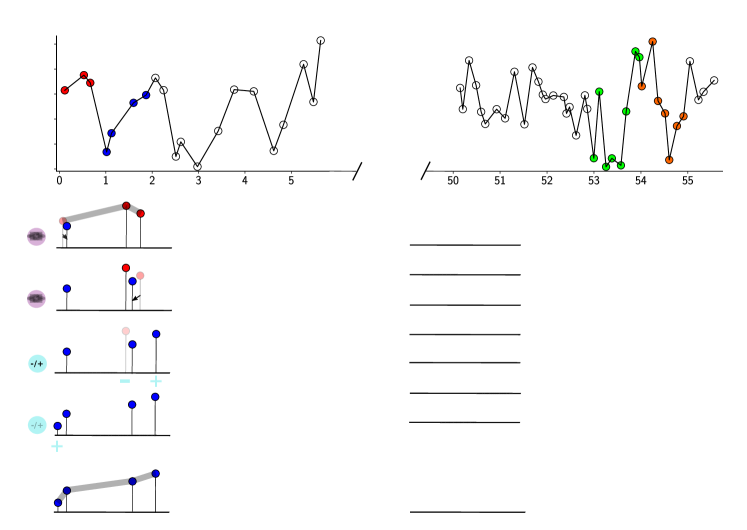
Figure 1: Schematic illustration of how irregularly sampled segments of varying lengths are transformed with the (m)Edit-distance method. Two exemplary pairs of segments $\mathcal{S}_{a},\,\mathcal{S}_{b}$ (A: red, blue) and $\mathcal{S}_{c},\,\mathcal{S}_{d}$ (B: green, orange) of an irregularly sampled synthetic AR(1)-time series are displayed. Each row shows an operation applied to the respective segment (shift: purple, deletion/adding: cyan). Final costs $C$ and $\tilde{C}$ result from a specific choice of cost parameters as described in Sect. II.1. Please note that the higher total cost in B showcase the dependence on segment length.

Irregular time axes are generated from a $\gamma(\Delta;k,\Theta)$-distribution with scale $\Theta$ and shape $k=\sqrt{\left.2\middle/\Gamma\right.}\,$, where $\Gamma$ denotes the skewness of the distribution. This choice is motivated by the observation that sampling intervals in palaeoclimate proxy time series are often $\gamma$- rather than exponentially-distributed. For each system, we generate a ‘superpopulation’ $(K=100)$ of time series and time axes. Fixing a different skewness $\Gamma$ of the $\gamma\,$-distribution of each of the time axes between $\Gamma\in[1,8]$ ensures that for $T=10,000$, segment sizes range between $N\in[1,20]$. The modified edit-distance is used, Eq. (1) and deletions are included as a competing operation to shifting. The optimal $\Lambda_{\mathrm{S}}$ is estimated for each system according to the procedure outlined in Sect. II.1: the KS-statistic is minimized for each systems, yielding $\Lambda^{{(\mathrm{unif})}}_{\mathrm{S}}=1.5,\,\Lambda^{{(\mathrm{AR1})}}_{\mathrm{S}}=1.5,\,\Lambda^{{(\mathrm{sin})}}_{\mathrm{S}}=3.5$.

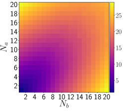
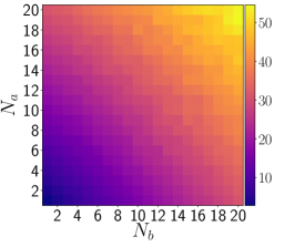
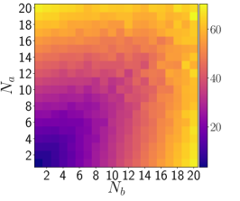
(a) Cost matrices ${{C}}(N_{a},N_{b})$ (including basic deletions, total costs).

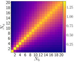
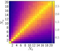
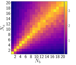
(b) Cost matrices ${{\tilde{C}}}_{\mathrm{shift}}(N_{a},N_{b})$ (excluding basic deletions, average costs per operation).

Figure 2: Cost matrices ${{C}}(N_{a},N_{b})$ for the transformation of segments with different lengths, including basic deletions (a) and excluding basic deletions (b). Costs are shown for uncorrelated uniform-distributed noise (left), an AR(1)-process (center) and a sinusoidal with superimposed white noise (right). Sampling intervals are $\gamma\,$-distributed.

Figure 2(a) displays the obtained transformation costs in the cost matrices ${{C}}(N_{a},N_{b})$ and ${{\tilde{C}}}_{\mathrm{shift}}(N_{a},N_{b})$ after averaging over $K=100$ different realizations. Regardless of the irregularity of the time axis and the respective system, a tendency of increasing total costs for larger segment sizes is observed (upper row). For the AR(1)-system, this increase is slower for fixed $N_{b}$ and increasing $N_{a}$ composed to the uncorrelated noise and the sinusoidal examples. More generally, the rate of increase differs between the considered systems but follows the same trend. In total, $|N_{a}-N_{b}|$ ‘basic deletions’ (or adding operations) need to be carried out for each pair of segments with $N_{a}\neq N_{b}$. If costs for these basic deletions are subtracted and computed per shifting step, a similar dependency on $N_{a},\,N_{b}$ as observed in Fig. 7c for the more simple case can be observed in the cost matrices ${{\tilde{C}}}_{\mathrm{shift}}(N_{a},N_{b})$ in Fig. 2(b) : the cost of an average shift from a segment with $N=N_{a}$ increases towards $N_{b}=N_{a}$ and decays if segment size increases further. Consequently, the leading effect results from the basic deletions that are directly linked to the difference in segment sizes $|N_{b}-N_{a}|$. Yet, transformation costs still depend on segment size even after aligning both segment sizes by means of basic deletions; this effect likely results from having a higher probability of finding closely spaced values on the time axis as the sampling rate of one segment increases, yielding an increasing trend for average costs per operation (in fig. 2(b)).

IV Sampling rate constrained surrogates

Irregularly sampled time series with constant sampling rate can be studied with the (m)Edit-distance to obtain dissimilarity estimates between different time series segments. The resulting distance matrix can be used to perform a recurrence analysis. Moreover, other analysis techniques such as complex networks, clustering, or correlation analysis are based on (dis)similarity measures and could use the (m)Edit-distance as a metric to account for irregular sampling or to characterize event-like data. In section III we showed that in case of a non-constant sampling rate, an estimation of the (m)Edit-distance matrix is biased by significant differences in the segment sizes.

In the following, we propose a numerical correction-technique for recurrence analysis. We generate an ensemble of time series and time axis surrogates that reproduces the sampling properties of the real irregularly sampled time series. This surrogate ensemble is used for bias-correction of recurrence quantification measures, exemplified by the determinism DET.

IV.1 Constrained randomization

When studying a system’s dynamics with time series analysis tools, a null-hypothesis is formulated which can be be tested. In case of recurrence analysis, this hypothesis could for example be non-stationarity of a dynamical property of the system (predictability, serial/cross-dependence, …) expressed by a particular recurrence quantification measure. In the used example, the null-hypothesis tests whether the observed dynamics could be solely caused by variations in the sampling rate.

Parametric hypothesis testing for time series analysis often poses severe constraints on the statistical properties of the underlying probability distribution, e.g., normality. Surrogate tests represent a non-parametric and flexible method to test for a range of properties in a system, including nonlinearity or periodicity, among others [56]. Time series surrogates are altered copies of a real, underlying time series that only preserve a specified set of properties of the real time series. The general technique to generate surrogate realizations of a time series is constrained randomization. After defining a set of constraints that state which properties of the real time series should be preserved, the time series is randomized such that these constraints are still fullfilled. Here, randomization will be carried out on the sampling interval $\Delta_{i}$ with the constraint that for each segment $\mathcal{S}_{i}$ of the real time series, segment size $N_{i}$ is preserved. This is achieved by drawing sampling intervals $\Delta_{i}$ (with replacement) from the empirical sampling interval distribution $p(\Delta,\lambda(t))$. For a given segment $S_{i}$ with size $N_{i}$, $N_{i}$ sampling intervals are drawn from $p(\Delta,\lambda(t))$ and cumulated to generate a surrogate realization of the particular time axis segment:

$$\tilde{t}_{\mathcal{S}_{i}}^{(0)}=t_{\mathcal{S}_{i}}^{(0)}\,,\quad\tilde{t}_{\mathcal{S}_{i}}^{(j+1)}=\tilde{t}_{\mathcal{S}_{i}}^{(0)}+\sum_{m=0}^{j}\Delta_{i}^{(m)}$$ (8)

Let $w$ be the time period covered by each segment. For any randomly sampled set of sampling intervals, the constraint of preserved segment size requires that

$$\tilde{t}_{\mathcal{S}_{i}}^{(N_{i})}\stackrel{{\scriptstyle\text{!}}}{{\leq}}w,$$ (9)

otherwise the random sampling of sampling intervals $\Delta_{i}$ has to be repeated. If the distribution of segment sizes is short-tailed, i.e., no segments with size $N\gg\mathbb{E}[k]$ exist, this simple randomization procedure converges rapidly for each segment. If segments of relatively large size are present – which is likely the case for non-stationary sampling rates – only a small subset of sampling intervals from the left tail of $p(\Delta,\lambda(t))$ will fulfill the condition (9). In order to ensure convergence of the algorithm for large segments, a weight-function can be introduced for all sampling intervals to increase the likelihood of drawing short sampling intervals when a segment with large size is generated. We suggest the use of $\beta$-distributed weights $\omega$:

$$\omega(X;\,\alpha,\beta)\,=\,\frac{1}{B(\alpha,\beta)}x^{\alpha-1}(1-x)^{\beta-1}$$ (10)

with the $\beta$-function $B(\alpha,\beta)$. This choice is motivated by the fact that for $\alpha=\beta=1$, $\omega(X;\,\alpha,\beta)$ becomes a uniform distribution. In our application, we choose $\alpha=\beta=1$ when the first iteration of sampling $N_{i}$ sampling intervals $\Delta_{i}$ is carried out. The population of sampling intervals is ordered from shortest to largest and each $x_{i}\leftrightarrow\Delta_{i}$ is assigned a $\beta$-distributed weight $\omega_{i}$, i.e., for the first iteration, every sampling interval is drawn with equal probability. If the iteration fails $\left(\tilde{t}_{\mathcal{S}_{i}}^{(N_{i})}>w\right)$, $\alpha$ is increased by a small number $\Delta\alpha$, reshaping the beta-distribution and increasing the probability of drawing small sampling intervals. Thus, we perform a weighted sampling from the empirical distribution $p(\Delta,\lambda(t))$ of sampling intervals with $\beta$-distributed weights. In the $l$-th iteration, we use $\omega(X;\,\alpha_{l},\beta=1),\,\alpha_{l}=1+l\Delta\alpha$ as the weight function for each segment. Finally, we can identify an amplitude difference $\Delta y_{i}$ of the time series with each sampling interval $\Delta_{i}$. This correspondence is exploited by also drawing the respective amplitude difference for each drawn sampling interval. After the procedure is finalized and a surrogate has been generated, amplitude differences are cumulated, that yields both a time axis and time series surrogate. Both are denoted as sampling rate constrained surrogate (SRC-surrogates). The full randomization procedure thus preserves segment sizes in the correct temporal order and by definition approximately reproduces the distribution of amplitude differences and sampling intervals.

It also preserves the correspondance between sampling intervals and amplitude differences, ensuring that if periods with high local sampling rate entail larger variance/strong amplitude changes in a real time series, this property is also included in the SRC-surrogates. The full procedure is outlined in Fig. 3 for an exemplary time series. Other randomization schemes are conceivable, e.g., varying the sampling weights after drawing each single sampling interval based on the size of the latter, or stratified randomization, i.e., performing the randomization differently for strata that correspond to the different segment sizes. However, the proposed scheme has proven to be effective within the scope of this work.

With the presented scheme of generating SRC-surrogates, an ensemble of surrogates can be generated and (m)Edit-distance matrices $\mathbf{D}$ computed for each SRC-surrogate. Any measure that is based on $\mathbf{D}$ can consequently be computed for each surrogate separately, yielding a distribution that can be used for testing the null-hypothesis formulated above based on the desired $\alpha$-confidence level.

IV.2 Recurrence analysis of an AR(1)-process

In the example below, the proposed correction scheme is applied to an irregularly sampled AR(1)-process (Fig. 5a). We consider an autocorrelation increasing with time, visible by autocorrelation time $\tau$ (Fig. 5b). A recurrence analysis is used to characterize the predictability of the time series in a sliding window analysis. Predictability is computed by means of determinism, DET, as defined in Eq. (7). In particular, we study how an abrupt shift of the sampling rate (represented by the skewness of $\gamma$-distributed sampling intervals) affects DET and if a continuous increase of predictability can be recovered despite this shift by using the proposed SRC-surrogate method. The shift appears at $t=1250$ (visible by variation of the segment size, Fig. 5b).

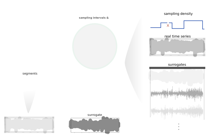
Figure 3: Schematic illustration of the constrained randomization procedure that generates SRC-surrogates for an exemplary irregularly sampled time series with non-stationary sampling rate. The left column shows the segmentation of the time series into segments of constant time period $s$ but of variable size $N_{i}$. The center column illustrates the weighted sampling of sampling intervals and amplitude differences. Each sampling interval is assigned a $\beta\,$-distributed weight whereby the $\alpha$-parameter of the weight distribution is increased with each $l$-th failed iteration to favor short sampling intervals. The resulting surrogates preserve the empirical distributions and segment sizes. Since amplitude differences are sampled jointly with the respective sampling intervals, increased volatility simply due to a higher local sampling rate is reproduced by the SRC-surrogates.

We expect DET to reproduce the linear increase in autocorrelation time, because increased serial dependence implies longer and more diagonal lines in the RP. For the computation of the (m)Edit-distance measure, segments are picked such that each covers a constant time interval of $w=1$ which could correspond to a year in a real-world application. 200 SRC-surrogates are generated (see appendix B) with $\alpha_{0}=1,\beta=1$ and a step size for the shape parameter $\alpha$ of the beta-distribution $\Delta\alpha=0.15$. We set an upper limit of $N_{\mathrm{it}}^{(\mathrm{max})}=1000$ for the number of iterations in the generation of each segment which is never exceeded in the performed simulations. The deletion/adding cost parameter $\Lambda_{S}$ is estimated separately for the real time series and the surrogate realizations, yielding $\Lambda_{S}^{(\mathrm{real})}=5.3$ and $\Lambda_{S}^{(\mathrm{SRC})}=2.6$. Recurrence plots are computed on sliding windows of size $s=200\Delta$ with $75\%$ overlap (time series length: $T=5000$). We fix a recurrence rate of $15\%$ and do not apply any time-delay embedding. For each window, two DET values are obtained (Fig. 5c): the DET value of the real time series and the $\alpha(=95\%)$-confidence level of DET values calculated from the SRC-surrogate ensemble. The DET measure indicates a spurious transition of predictability induced by the abrupt shift in sampling rate (Fig. 5c, grey shading). Both the real time series and the surrogate ensemble indicate this shift, demonstrating that the proposed SRC-surrogates effectively reproduce the sampling bias.

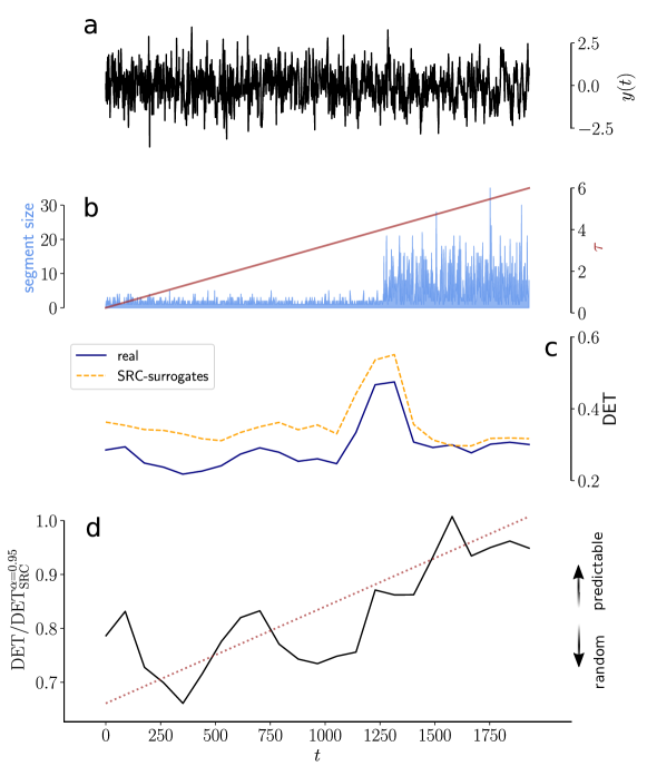
Figure 4: Application of SRC-surrogate correction method to (a) an irregularly sampled AR(1)-process with (b) non-stationary sampling rate (blue) and linearly increasing autocorrelation time (red). Gray shading indicates the abrupt shift in sampling rate. (c) A sliding window RQA using determinism (DET) as a predictability measure is carried out. Real DET values are displayed in dark blue, the $95\%$-confidence level computed from 200 SRC-surrogates is shown in yellow. (d) The ratio $\mathrm{DET}_{\mathrm{real}}$ by $\mathrm{DET}_{\mathrm{surr}}$ provides a sampling-bias corrected predictability measure that reproduces the linear increase in serial dependence.

The SRC-based correction is applied to DET values by dividing the real DET-series by the $95\%$-confidence level for each window (Fig. 5d). The resulting predictability estimates reproduce the expected linear increase in serial dependence whilst eliminating the spurious shift due to the jump of the sampling rate.

V Real-world application: rainfall seasonality in the central Pacific

Many real-world proxy time series are characterized by irregular sampling or missing data and stationarity of the underlying process that controls the sampling rate cannot be guaranteed. This perspective even goes beyond uneven time axes as for some systems, it might be desirable to apply an adaptive windowing in order to obtain segments with segment sizes depending on specific parameters of the system. For instance, when analyzing cardiac time series it might be reasonable to choose the segment size adaptively to capture one heart-beat cycle within each segment. The length of every cycle is controlled by a variety of other physical, non-stationary parameters. Below, we focus on an irregularly sampled palaeoclimate proxy time series with a non-stationary temporal sampling rate. We demonstrate the effectiveness of the proposed approach by carrying out a sliding window recurrence analysis.

The palaeoclimate record analysed here is a seasonally resolved stalagmite proxy record from Niue Island in the southwestern Pacific (19^∘S, 169^∘W). It covers 1000 years in the mid-Holocene (6.4-5.4 thousand years before present (ka BP)). Niue island has a tropical climate, receiving an average of 2000 mm of precipitation annually with a pronounced wet season from November to April. Rainfall is most strongly controlled by seasonal displacement of the South Pacific Convergence Zone but also reacts sensitively to atmospheric circulation changes associated with the El Niño-Southern Oscillation. Here, we analyse seasonal rainfall variability on Niue recorded in greyscale changes that arise from crystallographic variations caused by changes in the stalagmite growth rate (Fig. 6). Greyscale values are obtained from high resolution scans of the stalagmite surface along its growth axis subsequently extracted with ImageJ [57]. During the dry season, low drip rates promote the deposition of layers with compact and dark crystals, yielding low greyscale values. In the wet season, the drip rates are higher and crystal growth is enhanced as dissolved inorganic carbon is supplied to a greater extent. (see Fig. 6). The inferred link between dark layers and dry season is supported by earlier studies [58] [59].

Prior to the recurrence analysis of the greyscale time series, we subtracted a centennial-scale trend using a Gaussian kernel filter in order tp focus on the high-frequency variability in the record (Fig. 6a, black line). Next, we downsampled the time series uniformly by only storing every 10${}^{\text{th}}$ value due to computational constraints. This downsampling does not alter the relative changes in the sampling rate (Fig. 6b). The number of samples per year (i.e., the segment size) undergoes an abrupt shift at $\approx\,$6.15 ka BP. The period with the highest average segment size ($\approx\,$ 6.4 to 6.15 ka BP) coincides with the wettest period covered by the record, indicated by high greyscale values. This suggests that during this wet period, stalagmite growth was enhanced which resulted in thicker crystal laminae and a higher number of samples per layer. This observation reflects the complex nature of irregular sampling of palaeoclimate-proxy data. If spatial sampling on the stalagmite is performed such that the number of samples is as high as possible, it will inevitably be linked to its growth rate and thus to other environmental parameters and their non-stationary characteristics.

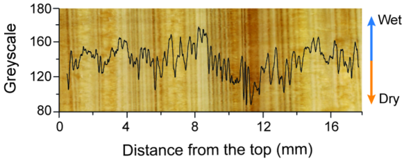
Figure 5: Greyscale record (in black) extracted from a high resolution scan of the surface of the stalagmite C132 from Niue island. Lower grey values are associated with dense microcrystalline calcite layers that form during drier periods.

Finally, we perform the recurrence analysis (Fig. 6c). In order to characterize seasonal features, the period covered by one segment is fixed as one year. Optimization of deletion/adding costs yields $\Lambda_{s}=2$. A window size of $s=200\,\mathrm{years}$ is chosen with $90\%$ overlap. A recurrence plot with fixed recurrence rate of $15\%\,$ is obtained for each window and analyzed with DET. DET reveals variations in seasonal-scale predictability for the real greyscale record (Fig. 6c, blue line). The effect of the varying sampling size is obtained by the $95\%\,$-quantile of the DET distribution from 200 SRC-surrogates (Fig. 6c, yellow line). Five exemplar SRC-surrogate realizations are shown in appendix B. Both DET time series indicate an increase of seasonal-scale predictability during the wet period between 6.35 to 6.2 ka BP, potentially caused by the simultaneously increased sampling rate. The predictability estimate is corrected for the identified sampling bias by considering the ratio $\mathrm{DET}_{\mathrm{r}}/\mathrm{DET}_{\mathrm{surr}}$ (Fig. 6d). Two periods (6.4 and 6.2 ka BP, and between 5.9 and 5.72 ka BP) show relatively low segment size-corrected seasonal predictability $\left.\mathrm{DET}_{\mathrm{r}}\middle/\mathrm{DET}_{\mathrm{surr}}\right.<1$. While the latter is not significantly affected by the correction, the former can only be identified as less predictable when the variations in sampling rate are taken into account. This result corroborates previous findings that suggested that both of these identified periods were more irregular, i.e. showing less steady seasonal fluctuations [59]. However, it was not possible to characterize all sub-annual values as a proxy for sub-annual rainfall distribution rather extracting only the contrast between wet and dry season. The (m)Edit-distance approach employed here in combination with the proposed correction technique allows for a more reliable interpretation of mid-Holocene seasonal variations in the west Pacific.

In particular, an enhanced control of the seasonal cycle by ENSO-scale variability was found in [59] for the periods of reduced predictability (6.4 and 6.2 ka BP, and between 5.9 and 5.72 ka BP). High tropical cyclone activity between 6.4-6.2 ka BP could have been triggered by increased ENSO activity, yielding a more irregular sub-annual distribution of rainfall. Our results indicate that not only contrast between both seasons is rendered less predictable during this period but also the seasonal rainfall distribution appears less stable from one year to another. Reconstructing past climate variability at seasonal scale plays a critical role in the context of human adaption to continuous and abrupt climate variations and therefore our approach has direct relevance for teasing out the seasonal-scale signals.

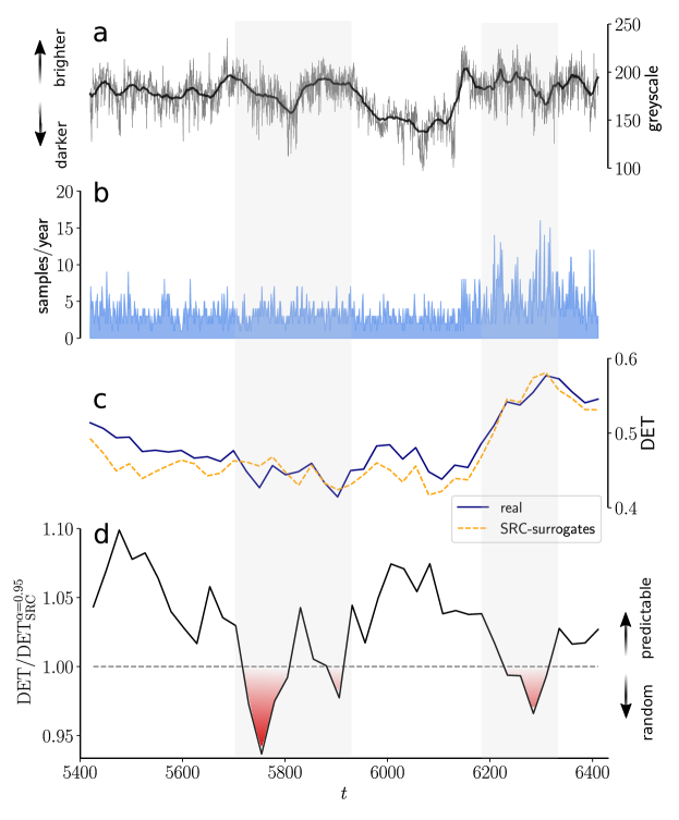
Figure 6: Application of SRC-surrogate correction method to an irregularly sampled greyscale proxy-record from the central Pacific (a) with non-stationary sampling rate (blue) (b). A sliding window RQA using determinism (DET) as a predictability measure is carried out (c). Real DET values are displayed in dark blue, the $95\%\,$-confidence level computed from 200 SRC-surrogates is shown in yellow. Dividing $\mathrm{DET}_{\mathrm{real}}$ by $\mathrm{DET}_{\mathrm{surr}}$ yields a sampling-bias corrected predictability series (d) that indicate mid-Holocene variations in seasonal-scale predictability. Gray shading indicates two periods with low seasonal predictability.

VI Conclusion

The characterization of time series from complex nonlinear systems is a challenging task. Irregular sampling, i.e., variations in the sampling interval between consecutive values, additionally impedes typical research objectives such as spectral analysis, persistence estimation or quantifying the predictability of a system. Even though interpolation techniques offer a seemingly efficient way of pre-processing a time series to allow application of standard time series analysis tools, these entail various biases which are difficult to control. A different perspective is pursued by the (m)Edit-distance method. Many analysis methods are based on an estimate of (dis)similarity. With the (m)Edit-distance, a suitable distance measure between states of a system at different times $i$ and $j$ is defined by computing the transformation cost of segments centered at these time instances. First analyses demonstrated its scope in the context of recurrence analysis, enabling researchers to examine predictability variations of irregularly sampled palaeoclimate time series. Applications to other complex systems (also for time series with ‘missing values’) and other methodological frameworks (e.g., complex networks, clustering, correlation analysis, …) are possible and should be attempted in the near future.

For some real-world systems, it is instructive to quantitatively compare sequences corresponding to a specific time scale in order to analyse the scale-specific variability. In such cases, segment sizes will vary in the presence of irregular sampling. Furthermore, splitting time series with a non-stationary sampling rate into segments that do not cover the same time period will result in a mixing of time scales. We have shown that (m)Edit-distance-based recurrence analyses are affected by variations in segment sizes, resulting in a non-trivial sampling bias if episodes with variable sampling rate are included in a single RP. The (m)Edit distance regards pairs of longer segments to be generally more dissimilar than shorter segments due to higher deletion costs. Shifting costs conversely decrease for increasing segment size, resulting in a non-trivial dependence of costs on local sampling rates. When including amplitudes of a signal into the (m)Edit-distance computation, similar general tendencies were observed but the strength of the segment size-dependencies varied for different systems. A more detailed examination of how dissimilar amplitude segments of different paradigmatic systems depend on their time scale will be investigated in a future study.

We introduced a numerical technique based on constrained randomization to address and correct the issue of segment-size dependence in recurrence analysis. This method involves generating an ensemble of sampling rate constrained surrogate realizations (SRC-surrogates). Each SRC-surrogate reproduces the real variations of sampling rate and its assignment to the corresponding amplitude differences, allowing the ensemble to be used for correcting the undesired segment size-dependence. The effectiveness of the proposed correction was applied to a synthetic AR(1)-time series and real palaeo-proxy data. In both applications, a recurrence analysis successfully recovered variations in the scale-specific predictability of the system whilst discarding spurious effects imprinted by sampling rate variations. We found that seasonal-scale predictability varied significantly during the mid-Holocene in the West Pacific, corroborating and extending the results from a recent study. The reasons for these changes in predictability warrant further investigation.

The identified sampling bias is a specific case of a more general problem in time series analysis; sliding window analyses (or the study of short time series) often suffer from finite-sampling biases which may introduce artificial variability into any statistical indicator that is computed. As pointed out in Section V, finite-sampling biases are also not limited to irregular temporal sampling but are likely to also occur in settings where other parameter axes determine suitable window sizes or adaptive windowing is required. In future, the proposed method could also be appliedd in such settings to test its effectiveness beyond the examples considered in this study.

Code availability

Python code for the generation of SRC-surrogates is available at https://github.com/ToBraun/SRC-surrogates.

Conflict of interest

The authors declare that they have no conflict of interest.

Appendix A: analytical and numerical segment size relations

In the following, we elaborate on the systematic dependence of the (m)Edit distance on segment lengths $N_{a}=|\mathcal{S}_{a}|,\,N_{b}=|\mathcal{S}_{b}|$ in the most simple application: we study events (i.e., no assumptions about the amplitude of the signal) which are unevenly spaced by exponentially distributed sampling intervals $\Delta$ with a sampling rate $\lambda$:

$$p(\Delta,\lambda)\,=\,\lambda\text{e}^{-\lambda\Delta}$$ (11)

Consequently, the number of samples per unit interval $k$ is Poisson-distributed

$$\rho(k,\lambda)\,=\,\frac{\lambda^{k}\mathrm{e}^{-k}}{k!}$$ (12)

with $\lambda$ being equivalent to the expected number of samples per unit interval; $\mathbb{E}(X)=\lambda$. Furthermore, the $n$-th time step is Erlang-distributed with the rate parameter $\lambda$:

$$f(t;n,\lambda)\,=\,\frac{\lambda^{n}t^{n-1}\mathrm{e}^{-\lambda t}}{(n-1)!}$$ (13)

which is a general result for a sum of $n$ independent exponential random variables with equivalent rate parameters $\lambda$ [60].

We are interested in the segment size-dependence of deletion(/adding) and shifting costs for the edit distance. This can be evaluated by considering $M$ exponential random variables where each is drawn from a distribution $p(\Delta,\lambda_{m})$ with distinct $\lambda_{m},\,m=1,2,\dots,M$. When applied, this setting can be considered equivalent to a scenario where a time axis changes its local sampling rate $\lambda_{m}$ at $M$ points and segments from these should be compared via the edit-distance. For a specific pair of segments with sizes $N_{a},N_{b}$, the minimum deletion cost (no deletions as competing to shifts included) for their transformation is

$$C_{\mathrm{del}}(N_{a},N_{b})\,=\,\Lambda_{\mathrm{S}}|N_{a}-N_{b}|$$ (14)

Consequently, for two segments of average sizes $\mathbb{E}[N_{a}]=\lambda_{1},\,\mathbb{E}[N_{b}]=\lambda_{2}$ we obtain a minimum deletion cost of $C_{\mathrm{del}}\left(\mathbb{E}(N_{a}),\mathbb{E}(N_{b})\right)\,=\,\Lambda_{\mathrm{S}}|\lambda_{1}-\lambda_{2}|$. A cost matrix $C_{\mathrm{del}}(\lambda_{1},\lambda_{2})$ is exemplified in Fig. 7a. The expected minimum deletion cost for two randomly selected segments from time periods with different rates $\lambda_{1},\,\lambda_{2}$ can be computed by using the the Skellam distribution

$$\rho_{s}(k=|z|;\lambda_{1},\lambda_{2})\,=\,\left\{\begin{array}[]{ll}\mathrm{e}^{-\lambda_{1}-\lambda_{2}}\left((\frac{\lambda_{1}}{\lambda_{2}})^{\frac{k}{2}}I_{k}(2\sqrt{\lambda_{1}\lambda_{2}})\,+\,(\frac{\lambda_{2}}{\lambda_{1}})^{\frac{k}{2}}I_{-k}(2\sqrt{\lambda_{1}\lambda_{2}})\right)&\mathrm{if}\,k>0\\ \mathrm{e}^{-\lambda_{1}-\lambda_{2}}I_{0}(2\sqrt{\lambda_{1}\lambda_{2}})&\mathrm{if}\,k=0\end{array}\right.$$ (17)

for the difference $Z=X-Y$ where $X,\,Y$ are Poisson-distributed random variables with rates $\lambda_{1},\,\lambda_{2}$, Eq. (12). $I_{k}(a)$ denotes the modified Bessel function of the first kind. For $k>0$, the moment-generating function is consequently given by

$$\begin{split}M(t;\lambda_{1},\lambda_{2})\,=\,&\mathrm{e}^{-\lambda_{1}-\lambda_{2}}\left(\sum_{k=0}^{\infty}\mathrm{e}^{tk}I_{k}(2\sqrt{\lambda_{1}\lambda_{2}})\right.\\ &\left.\left[\left(\frac{\lambda_{1}}{\lambda_{2}}^{k/2}\right)+\left(\frac{\lambda_{2}}{\lambda_{2}}^{k/2}\right)\right]-I_{0}(2\sqrt{\lambda_{1}\lambda_{2}})\right)\end{split}$$ (18)

With ‘Marcum’s Q’

$$Q(\sqrt{2\lambda_{1}},\sqrt{2\lambda_{2}})=\mathrm{e}^{-\lambda_{1}-\lambda_{2}}\sum_{k=0}^{\infty}\left(\frac{\lambda_{1}}{\lambda_{2}}\right)^{\frac{k}{2}}I_{k}(2\sqrt{\lambda_{1}\lambda_{2}})$$ (19)

and its derivative

$$\begin{split}\dfrac{\mathrm{d}}{\mathrm{d}t}Q(\sqrt{2\lambda_{1}},\sqrt{2\lambda_{2}})\,=\,\mathrm{e}^{-\lambda_{1}\mathrm{e}^{t}-\lambda_{2}\mathrm{e}^{-t}}\left(\lambda_{2}\mathrm{e}^{-t}I_{0}(2\sqrt{\lambda_{1}\lambda_{2}})+\right.\\ \left.\sqrt{\lambda_{1}\lambda_{2}}I_{1}(2\sqrt{\lambda_{1}\lambda_{2}})\right)\end{split}$$ (20)

this can be written as

$$\begin{split}M(t;\lambda_{1},\lambda_{2})\,=\,\mathrm{e}^{-\lambda_{1}-\lambda_{2}}\left[Q\left(\sqrt{2\lambda_{2}\mathrm{e}^{-t}},\sqrt{2\lambda_{1}\mathrm{e}^{t}}\right)\mathrm{e}^{\lambda_{1}\mathrm{e}^{t}+\lambda_{2}\mathrm{e}^{-t}}\right.\\ \left.Q\left(\sqrt{2\lambda_{1}\mathrm{e}^{-t}},\sqrt{2\lambda_{2}\mathrm{e}^{t}}\right)\mathrm{e}^{\lambda_{2}\mathrm{e}^{t}+\lambda_{1}\mathrm{e}^{-t}}I_{0}(2\sqrt{\lambda_{1}\lambda_{2}})\right]\end{split}$$ (21)

Differentiating this moment-generating function (using eq. 20) around $t=0$ with Leibniz rule yields the expected value:

$$\begin{split}\mathbb{E}[k;\lambda_{1},\lambda_{2}]\ =\ &2\mathrm{e}^{-\lambda_{1}-\lambda_{2}}\left(\lambda_{2}I_{0}(2\sqrt{\lambda_{1}\lambda_{2}})+\sqrt{\lambda_{1}\lambda_{2}}I_{1}(2\sqrt{\lambda_{1}\lambda_{2}})\right)\\ \,+\,&\left(\lambda_{2}-\lambda_{1})(1-2Q(\sqrt{2\lambda_{1}},\sqrt{2\lambda_{2}})\right)\end{split}$$ (22)

Hence, $\mathbb{E}[C_{\mathrm{del}}(\lambda_{1},\lambda_{2})]\,=\,\Lambda_{\mathrm{S}}\mathbb{E}[k;\lambda_{1},\lambda_{2}]$ (Fig. 7a (middle)). In the right line plot of Fig. 7a, two columns with $\lambda_{1}$ fixed at $3.1$ are shown to illustrate the scaling of deletion costs with the rate $\lambda$ more clearly. While $C_{\mathrm{del}}\left(\mathbb{E}(N_{a}),\mathbb{E}(N_{b})\right)$ shows a sharp minimum at the rate $\lambda_{2}=\lambda_{1}$, $\mathbb{E}[k;\lambda_{1},\lambda_{2}]$ decreases more smoothly with increasing $\lambda_{2}$, and increases afterwards. The latter becomes minimal for a value $\lambda<\lambda_{2}$ instead of $\lambda=\lambda_{2}$ since Poisson-distributions $\rho(k,\lambda)$ are right-skewed, having higher cumulated probability mass for all values $k>\lambda$. Note that all said above holds in the same way for adding operations.

For the analysis of shifting costs, we focus on the simple case of linear shifting costs

$$\tilde{f}_{\Lambda_{0}}\left(t(\alpha),t(\beta)\right)\,=\,|t(\alpha)-t(\beta)|$$ (23)

between the $\alpha$-th event in segment $\mathcal{S}_{a}$ and the $\beta$-th event in segment $\mathcal{S}_{b}$ as proposed in the original, unmodified edit-distance measure. To exclude effects caused by absolute timing of events, timing of events within each segment is always transformed into the interval $I=[0,1]$. The sum of all shifting costs for a pair of segments is denoted as $d_{ab}=\Lambda_{0}\sum_{\alpha,\beta}f_{\Lambda_{0}}\left(t(\alpha),t(\beta)\right)$ with $\Lambda_{0}=1$. Note that $N_{a}=N_{b}$ as $|N_{a}-N_{b}|$ deletions/addings have already been carried out. A closed-form solution for the shifting costs between two time instances drawn randomly from the distributions $f(x;m_{1},\lambda_{1}),\,f(y;m_{2},\lambda_{2})$ most likely exists, at least for the case $m_{1}=m_{2}$ but its computation is beyond this study. We examine shifting costs for this case numerically, while we explicitly exclude any deletions as an alternative operation to shifting after the neccessary $|N_{a}-N_{b}|$ deletions (‘basic deletions’) (Fig. 7b). We fix $w=1$ as the unit interval (arbitrary units). The numerical estimate of the average cost for transforming a segment sampled with rate $\lambda_{1}$ into a segment sampled with rate $\lambda_{2}$ is based on generating time axes for a fixed time period $T=10,000$ (but varying number of events). Given a fixed combination of $\lambda_{1},\,\lambda_{2}$, a total of $K=10,000$ segment pairs are randomly sampled (with replacement) from both corresponding time axes. The edit-distance is computed for each pair of segments and averaged over all pairs to obtain a single value $\overline{d}(\lambda_{1},\,\lambda_{2})$ that is characteristic for the combination of rates $\lambda_{1},\,\lambda_{2}$. This is shown as a cost matrix $C_{\mathrm{shift}}(\lambda_{1},\lambda_{2})$ of averaged total shifting costs between randomly drawn segments (Fig. 7b, left). The total number of shifts performed after deleting $|N_{a}-N_{b}|$ events generally differs for distinct pairs of segments $\mathcal{S}_{a},\mathcal{S}_{b}$ at fixed $\lambda_{1},\,\lambda_{2}$. However, when averaged over all randomly drawn segment pairs, an increasing trend along the diagonals is observed. Furthermore, average total shifting costs $\overline{d}(\lambda_{1},\,\lambda_{2})$ increase for fixed $\lambda_{1}$ and increasing $\lambda_{2}$ (Fig.7b, right) which is to be expected as a higher number of shifts will entail higher summed costs. On the other hand, no monotonous relation between the average shifting costs per shifting operation

$$\left.{{\tilde{C}}}_{\mathrm{shift}}(\lambda_{1},\lambda_{2})=\sum_{k=1}^{K}d(\mathcal{S}_{a,k}^{(\lambda_{1})},\,\mathcal{S}_{b,k}^{(\lambda_{2})})\middle/\mathrm{max}\{N_{a},N_{b}\}\right.$$ (24)

and sampling rate is observed (Fig. 7b, center and bold black line on the right). With increasing sampling rates, the cost of an average single shifting operation decreases (diagonals of the matrix). For fixed $\lambda_{1}$, it is maximized at a value $\lambda_{2}<\lambda_{1}$ for the same reason as above, i.e. the Erlang distribution being right-skewed.

If we instead examine the dependence of shifting costs on the actual segment size ${{\tilde{C}}}_{\mathrm{shift}}(N_{a},\,N_{b})$ rather than the rates (Fig. 7c), a sharp maximum at $N_{b}=\lambda_{1}$ is found (black line, right plot). Total shifting costs increase for $N_{b}<\lambda_{1}$ and continue to increase more slowly for $N_{b}>\lambda_{1}$. For fixed $N_{a}$, an increasing number $N_{b}$ of events per unit interval increases the likelihood that some events are placed close to the events in segment $\mathcal{S}_{a}$, resulting in lower distances $d_{ab}(N_{a},\,N_{b})$.

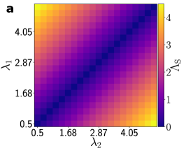
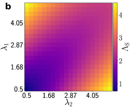
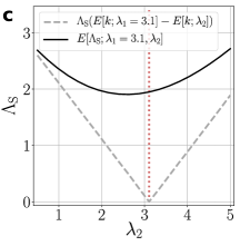
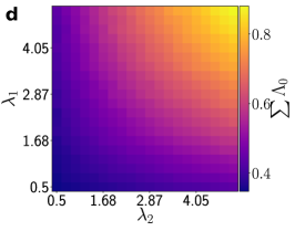
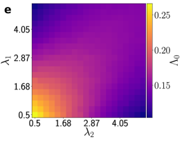
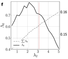
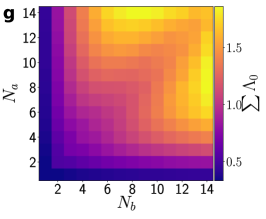
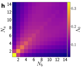
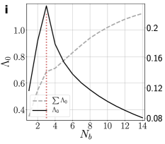
Figure 7: Subcosts for adding/deleting (a-c) and shifting (d-i) operations for exponentially distributed sampling intervals. Only necessary deleting/adding operations are regarded (‘no competing operations’). The sampling rate-dependence of deletion costs is given as difference between expected number of samples per unit interval (left matrix and grey dashed line) and as expected costs given two rates $\lambda_{1},\lambda_{2}$ (right matrix and black line, eq. (22)). Shifting costs are studied (b) numerically with respect to their dependence on the sampling rates $\lambda_{1},\,\lambda_{2}$ and (c) on the actual number of samples per unit interval $N_{a},\,N_{b}$. The left matrices shows shifting costs for the full transformation of segments, the center matrices show shifting costs per operation. Exemplary columns are displayed in the line plots whereas the red dashed line marks the respective rate $\lambda_{1}$/segment size $N_{b}$.

Appendix B: sampling rate-constrained surrogates

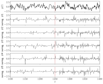
Figure 8: Zoomed section of synthetic AR(1)-time series (black) and five exemplar SRC-surrogate realizations (gray). The red dotted line indicates the transition of the sampling rate towards more dense sampling. Sampling intervals are $\gamma\,$-distributed.

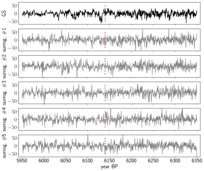
Figure 9: Zoomed section of grayscale anomaly time series (black) and five exemplar SRC-surrogate realizations (gray). The red dotted line indicates the transition of the sampling rate towards more dense sampling.

References

- [1] R. Renò, “A closer look at the epps effect,” International Journal of theoretical and applied finance, vol. 6, no. 01, pp. 87–102, 2003.
- [2] A. Fedotov, S. Akulov, and E. Timchenko, “Methods of mathematical analysis of heart rate variability,” Biomedical Engineering, vol. 54, no. 3, pp. 220–225, 2020.
- [3] C. K. Enders, Applied missing data analysis. Guilford press, 2010.
- [4] M. Khayati, A. Lerner, Z. Tymchenko, and P. Cudré-Mauroux, “Mind the gap: an experimental evaluation of imputation of missing values techniques in time series,” Proceedings of the VLDB Endowment, vol. 13, no. 5, pp. 768–782, 2020.
- [5] J. D. Scargle, “Studies in astronomical time series analysis. ii-statistical aspects of spectral analysis of unevenly spaced data,” The Astrophysical Journal, vol. 263, pp. 835–853, 1982.
- [6] K. Rehfeld, N. Marwan, J. Heitzig, and J. Kurths, “Comparison of correlation analysis techniques for irregularly sampled time series,” Nonlinear Processes in Geophysics, vol. 18, no. 3, pp. 389–404, 2011.
- [7] J. U. Baldini, “Detecting and quantifying paleoseasonality in stalagmites using geochemical and modelling approaches,” AGUFM, vol. 2017, pp. PP54B–09, 2021.
- [8] C. Mühlinghaus, D. Scholz, and A. Mangini, “Modelling stalagmite growth and 13c as a function of drip interval and temperature,” Geochimica et Cosmochimica Acta, vol. 71, no. 11, pp. 2780–2790, 2007.
- [9] J. Garland, T. R. Jones, M. Neuder, V. Morris, J. W. White, and E. Bradley, “Anomaly detection in paleoclimate records using permutation entropy,” Entropy, vol. 20, no. 12, p. 931, 2018.
- [10] M. H. Trauth, “Spectral analysis in quaternary sciences,” Quaternary Science Reviews, vol. 270, p. 107157, 2021.
- [11] K. Rehfeld, N. Marwan, S. F. Breitenbach, and J. Kurths, “Late holocene asian summer monsoon dynamics from small but complex networks of paleoclimate data,” Climate dynamics, vol. 41, no. 1, pp. 3–19, 2013.
- [12] M. Schulz and K. Stattegger, “Spectrum: Spectral analysis of unevenly spaced paleoclimatic time series,” Computers & Geosciences, vol. 23, no. 9, pp. 929–945, 1997.
- [13] N. V. Chawla, K. W. Bowyer, L. O. Hall, and W. P. Kegelmeyer, “Smote: synthetic minority over-sampling technique,” Journal of artificial intelligence research, vol. 16, pp. 321–357, 2002.
- [14] S. Barua, M. M. Islam, X. Yao, and K. Murase, “Mwmote–majority weighted minority oversampling technique for imbalanced data set learning,” IEEE Transactions on knowledge and data engineering, vol. 26, no. 2, pp. 405–425, 2012.
- [15] T. M. Lenton, J. Rockström, O. Gaffney, S. Rahmstorf, K. Richardson, W. Steffen, and H. J. Schellnhuber, “Climate tipping points—too risky to bet against,” 2019.
- [16] E. Bradley and H. Kantz, “Nonlinear time-series analysis revisited,” Chaos: An Interdisciplinary Journal of Nonlinear Science, vol. 25, no. 9, p. 097610, 2015.
- [17] N. Marwan, J. F. Donges, R. V. Donner, and D. Eroglu, “Nonlinear time series analysis of palaeoclimate proxy records,” Quaternary Science Reviews, vol. 274, p. 107245, 2021.
- [18] M. Scheffer, J. Bascompte, W. A. Brock, V. Brovkin, S. R. Carpenter, V. Dakos, H. Held, E. H. Van Nes, M. Rietkerk, and G. Sugihara, “Early-warning signals for critical transitions,” Nature, vol. 461, no. 7260, pp. 53–59, 2009.
- [19] J. Lekscha and R. V. Donner, “Phase space reconstruction for non-uniformly sampled noisy time series,” Chaos: An Interdisciplinary Journal of Nonlinear Science, vol. 28, no. 8, p. 085702, 2018.
- [20] M. McCullough, K. Sakellariou, T. Stemler, and M. Small, “Counting forbidden patterns in irregularly sampled time series. i. the effects of under-sampling, random depletion, and timing jitter,” Chaos: An Interdisciplinary Journal of Nonlinear Science, vol. 26, no. 12, p. 123103, 2016.
- [21] K. Sakellariou, M. McCullough, T. Stemler, and M. Small, “Counting forbidden patterns in irregularly sampled time series. ii. reliability in the presence of highly irregular sampling,” Chaos: An Interdisciplinary Journal of Nonlinear Science, vol. 26, no. 12, p. 123104, 2016.
- [22] S. Suzuki, Y. Hirata, and K. Aihara, “Definition of distance for marked point process data and its application to recurrence plot-based analysis of exchange tick data of foreign currencies,” International Journal of Bifurcation and Chaos, vol. 20, no. 11, pp. 3699–3708, 2010.
- [23] I. Ozken, D. Eroglu, T. Stemler, N. Marwan, G. B. Bagci, and J. Kurths, “Transformation-cost time-series method for analyzing irregularly sampled data,” Physical Review E, vol. 91, no. 6, p. 062911, 2015.
- [24] E. Ukkonen, “Algorithms for approximate string matching,” Information and control, vol. 64, no. 1-3, pp. 100–118, 1985.
- [25] A. Banerjee, B. Goswami, Y. Hirata, D. Eroglu, B. Merz, J. Kurths, and N. Marwan, “Recurrence analysis of extreme event like data,” Nonlinear Processes in Geophysics Discussions, pp. 1–25, 2020.
- [26] I. Ozken, D. Eroglu, S. F. Breitenbach, N. Marwan, L. Tan, U. Tirnakli, and J. Kurths, “Recurrence plot analysis of irregularly sampled data,” Physical Review E, vol. 98, no. 5, p. 052215, 2018.
- [27] N. Marwan, M. C. Romano, M. Thiel, and J. Kurths, “Recurrence plots for the analysis of complex systems,” Physics reports, vol. 438, no. 5-6, pp. 237–329, 2007.
- [28] E. Garcia-Ceja, M. Z. Uddin, and J. Torresen, “Classification of recurrence plots’ distance matrices with a convolutional neural network for activity recognition,” Procedia computer science, vol. 130, pp. 157–163, 2018.
- [29] M. C. Romano, M. Thiel, J. Kurths, and W. von Bloh, “Multivariate recurrence plots,” Physics letters A, vol. 330, no. 3-4, pp. 214–223, 2004.
- [30] N. Marwan, S. Schinkel, and J. Kurths, “Recurrence plots 25 years later—gaining confidence in dynamical transitions,” EPL (Europhysics Letters), vol. 101, no. 2, p. 20007, 2013.
- [31] G. Corso, T. d. L. Prado, G. Z. d. S. Lima, J. Kurths, and S. R. Lopes, “Quantifying entropy using recurrence matrix microstates,” Chaos: An Interdisciplinary Journal of Nonlinear Science, vol. 28, no. 8, p. 083108, 2018.
- [32] S. Schinkel, N. Marwan, and J. Kurths, “Order patterns recurrence plots in the analysis of erp data,” Cognitive neurodynamics, vol. 1, no. 4, pp. 317–325, 2007.
- [33] T. Braun, V. R. Unni, R. Sujith, J. Kurths, and N. Marwan, “Detection of dynamical regime transitions with lacunarity as a multiscale recurrence quantification measure,” Nonlinear Dynamics, pp. 1–19, 2021.
- [34] N. Marwan, D. Eroglu, I. Ozken, T. Stemler, K.-H. Wyrwoll, and J. Kurths, “Regime change detection in irregularly sampled time series,” in Advances in Nonlinear Geosciences, pp. 357–368, Springer, 2018.
- [35] M. A. Stegner, Z. Ratajczak, S. R. Carpenter, and J. W. Williams, “Inferring critical transitions in paleoecological time series with irregular sampling and variable time-averaging,” Quaternary Science Reviews, vol. 207, pp. 49–63, 2019.
- [36] K. H. Kraemer, G. Datseris, J. Kurths, I. Z. Kiss, J. L. Ocampo-Espindola, and N. Marwan, “A unified and automated approach to attractor reconstruction,” New Journal of Physics, 2021.
- [37] K. Rehfeld and J. Kurths, “Similarity estimators for irregular and age-uncertain time series,” Climate of the Past, vol. 10, no. 1, pp. 107–122, 2014.
- [38] M. Mudelsee, Climate time series analysis. Springer, 2013.
- [39] W. J. Masek and M. S. Paterson, “A faster algorithm computing string edit distances,” Journal of Computer and System sciences, vol. 20, no. 1, pp. 18–31, 1980.
- [40] L. Rabiner, A. Rosenberg, and S. Levinson, “Considerations in dynamic time warping algorithms for discrete word recognition,” IEEE Transactions on Acoustics, Speech, and Signal Processing, vol. 26, no. 6, pp. 575–582, 1978.
- [41] J. D. Victor and K. P. Purpura, “Metric-space analysis of spike trains: theory, algorithms and application,” Network: computation in neural systems, vol. 8, no. 2, pp. 127–164, 1997.
- [42] E. Jp, “Recurrence plots of dynamical systems,” Europhysics Ltters, vol. 5, pp. 973–977, 1987.
- [43] H. Poincaré, “Sur le problème des trois corps et les équations de la dynamique,” Acta mathematica, vol. 13, no. 1, pp. A3–A270, 1890.
- [44] K. H. Kraemer, R. V. Donner, J. Heitzig, and N. Marwan, “Recurrence threshold selection for obtaining robust recurrence characteristics in different embedding dimensions,” Chaos: An Interdisciplinary Journal of Nonlinear Science, vol. 28, no. 8, p. 085720, 2018.
- [45] S. Schinkel, O. Dimigen, and N. Marwan, “Selection of recurrence threshold for signal detection,” European Physical Journal – Special Topics, vol. 164, no. 1, pp. 45–53, 2008.
- [46] Y. Hirata, “Recurrence plots for characterizing random dynamical systems,” Communications in Nonlinear Science and Numerical Simulation, vol. 94, p. 105552, 2021.
- [47] A. M. Ramos, A. Builes-Jaramillo, G. Poveda, B. Goswami, E. E. Macau, J. Kurths, and N. Marwan, “Recurrence measure of conditional dependence and applications,” Physical Review E, vol. 95, no. 5, p. 052206, 2017.
- [48] T. Westerhold, N. Marwan, A. J. Drury, D. Liebrand, C. Agnini, E. Anagnostou, J. S. Barnet, S. M. Bohaty, D. De Vleeschouwer, F. Florindo, et al., “An astronomically dated record of earth’s climate and its predictability over the last 66 million years,” Science, vol. 369, no. 6509, pp. 1383–1387, 2020.
- [49] H. Kantz, “A robust method to estimate the maximal lyapunov exponent of a time series,” Physics letters A, vol. 185, no. 1, pp. 77–87, 1994.
- [50] R. V. Donner and S. M. Barbosa, “Nonlinear time series analysis in the geosciences,” Lecture Notes in Earth Sciences, vol. 112, 2008.
- [51] T. March, S. Chapman, and R. Dendy, “Recurrence plot statistics and the effect of embedding,” Physica D: Nonlinear Phenomena, vol. 200, no. 1-2, pp. 171–184, 2005.
- [52] D. C. Williams, “Finite sample correction factors for several simple robust estimators of normal standard deviation,” Journal of Statistical Computation and Simulation, vol. 81, no. 11, pp. 1697–1702, 2011.
- [53] C. Park, H. Kim, and M. Wang, “Investigation of finite-sample properties of robust location and scale estimators,” Communications in Statistics-Simulation and Computation, pp. 1–27, 2019.
- [54] K. E. Trenberth, “Some effects of finite sample size and persistence on meteorological statistics. part i: Autocorrelations,” Monthly Weather Review, vol. 112, no. 12, pp. 2359–2368, 1984.
- [55] B. Goswami, P. Schultz, B. Heinze, N. Marwan, B. Bodirsky, H. Lotze-Campen, and J. Kurths, “Inferring interdependencies from short time series,” in Indian Academy of Sciences Conference Series, vol. 1, pp. 51–60, 2017.
- [56] T. Schreiber and A. Schmitz, “Surrogate time series,” Physica D: Nonlinear Phenomena, vol. 142, no. 3-4, pp. 346–382, 2000.
- [57] M. D. Abràmoff, P. J. Magalhães, and S. J. Ram, “Image processing with imagej,” Biophotonics international, vol. 11, no. 7, pp. 36–42, 2004.
- [58] P. Aharon, M. Rasbury, and V. Murgulet, “Caves of niue island, south pacific: Speleothems and water geochemistry,” Geological Society of America Special Papers, vol. 404, pp. 283–295, 2006.
- [59] C. Nava-Fernandez, T. Braun, B. Fox, A. Hartland, O. Kwiecien, C. L. Pederson, S. N. Höpker, S. Bernasconi, M. Jaggi, J. Hellstrom, F. Gazquez, A. French, N. Marwan, A. Immenhauser, and S. Breitenbach, “Mid-holocene rainfall changes in the southwestern pacific,” Submitted to Climate of the Past, 2021.
- [60] D. R. Cox, Renewal theory. Springer, 1967.