Ab initio thermodynamics of one-component plasma for astrophysics of white dwarfs and neutron stars

Abstract

Using path-integral Monte Carlo (PIMC) simulations, we have calculated energy of a crystal composed of atomic nuclei and uniform incompressible electron background in the temperature and density range, covering fully ionized layers of compact stellar objects, white dwarfs and neutron stars, including the high-density regime, where ion quantization is important. We have approximated the results by convenient analytic formulae, which allowed us to integrate and differentiate the energy with respect to temperature and density to obtain various thermodynamic functions such as Helmholtz free energy, specific heat, pressure, entropy etc. In particular, we have demonstrated, that the total crystal specific heat can exceed the well-known harmonic lattice contribution by a factor of 1.5 due to anharmonic effects. By combining our results with the PIMC thermodynamics of a quantum Coulomb liquid, updated in the present work, we were able to determine density dependences of such melting parameters as the Coulomb coupling strength at melting, latent heat, and a specific heat jump. Our results are necessary for realistic modelling of thermal evolution of compact degenerate stars.

1 Introduction

Modelling evolution of white dwarfs (WD), in an attempt to understand their extremely diverse observational properties, is a hot topic of modern astrophysics. Thanks to Gaia (Gaia Collaboration et al., 2016), the wealth of experimental data, awaiting theoretical explanation, is rapidly growing. For instance, a population of WD called the Q branch on the Hertzsprung–Russell diagram has been recently discovered (Gaia Collaboration et al., 2018), which implies an $\sim 8$ Gyr cooling delay with respect to a standard evolutionary track (Cheng, Cummings & Ménard, 2019). Such a delay may be due to core crystallization accompanied by latent heat release and oxygen sedimentation in massive WD (Tremblay et al., 2019). Other sources of extra thermal energy associated with chemical separation and gravitational energy release in crystallizing matter have been also discussed (e.g. Bauer et al.,, 2020; Caplan, Horowitz & Cumming, 2020; Blouin, Daligault & Saumon, 2021; Camisassa et al.,, 2021; Blouin & Daligault, 2021; Caplan et al.,, 2021).

In this paper, we focus on microphysics of WD interior. Plasma in a WD core consists of fully ionized atomic nuclei and electrons. Its energy has three major terms (e.g. Haensel, Potekhin & Yakovlev 2007; Potekhin & Chabrier 2010; Baiko 2014; Oertel et al., 2017): the electron energy (the energy of a degenerate electron gas), the ion energy (the energy of an ion plasma with constant and uniform electron background), and the ion-electron energy (due to electron screening of inter-ion interactions).

The electron energy is a well studied quantity. Its main term is due to the ideal zero-temperature relativistic degenerate electron gas, and there are several higher-order corrections (thermal, exchange, correlation). By definition, at a given temperature and density, the electron contribution is identical regardless of whether ions constitute a liquid or a crystal (see below). For many thermodynamic quantities, such as pressure and energy, the electron contribution is dominant. However, specific heat and temperature derivative of pressure are dominated by ions. The latter quantities are crucial for thermal evolution and asteroseismology of WD.

By contrast, the ion-electron thermodynamic functions are not known very reliably. They have been studied by two independent methods: perturbatively in the liquid (e.g. Potekhin & Chabrier, 2000) and within the framework of the harmonic lattice theory in the solid (e.g. Baiko, 2002). As stressed in the latter work, the two approaches yielded contradictory results, predicting, for instance, opposite signs of ion-electron corrections to the specific heat in liquid and solid phases near melting. This discrepancy remains one of the outstanding issues in the field of WD microphysics, however, the relative magnitude of these contributions is small, so that, most likely, it is inconsequential from the WD evolutionary theory perspective.

In what follows, we shall neglect the higher-order electron and the ion-electron contributions, focusing on the ion contribution and utilizing the standard thermodynamics of the ideal fully-degenerate electron gas only in Sec. 7.

The ion contribution to the thermodynamic quantities is nontrivial. The ion plasma with rigid charge-compensating background has been studied extensively, as it is a model system for a branch of plasma physics, dealing with strongly coupled Coulomb plasmas. If such a plasma contains ions of only one sort, it is called a one-component plasma (OCP). In general however, one expects a mixture of several ion species in WD interior, i.e. a multi-component plasma (for instance, a C/O mixture with traces of Ne). Both one- and multi-component plasmas have been studied by classic Monte Carlo and molecular dynamics methods (e.g. Stringfellow, Dewitt & Slattery 1990; Farouki & Hamaguchi 1993; Caillol 1999; Dewitt & Slattery 1999, 2003; Horowitz, Berry & Brown 2007; Horowitz, Schneider & Berry 2010; Caplan, Horowitz & Cumming 2020; Caplan 2020; Blouin & Daligault 2021). For instance, the first-order melting/crystallization phase transition between a liquid and a body-centered cubic solid in a classic ion OCP is well-known. It occurs at $\Gamma=\Gamma_{\rm m}\approx 175$ (e.g. Potekhin & Chabrier, 2000; Haensel et al., 2007), where $\Gamma=Z_{\mathrm{i}}^{2}e^{2}/(a_{\mathrm{i}}T)$ is the dimensionless Coulomb coupling parameter, $T$ is the temperature (the Boltzmann constant $k_{\rm B}\equiv 1$), $a_{\mathrm{i}}=(4\pi n_{\mathrm{i}}/3)^{-1/3}$ is the Wigner-Seitz radius, $n_{\mathrm{i}}$ and $Z_{\mathrm{i}}$ are the ion number density and charge number, respectively.

It has been long recognized, that treatment of ions as classic particles is not fully adequate in WD interior (e.g. Chabrier, Ashcroft & Dewitt, 1992). The most obvious illustration of this statement is given by a WD with a crystallized core undergoing Debye cooling (e.g. Ostriker & Axel 1968; Lamb & van Horn 1975). To the lowest order, the ion thermodynamics in this case is that of a low temperature Bose gas of phonons in a harmonic Coulomb solid (Kugler, 1969; Chabrier, 1993; Baiko, Potekhin & Yakovlev, 2001, hereafter the latter work will be referred to as Paper I). However, anharmonic corrections in the ion crystal are not negligible (e.g. Farouki & Hamaguchi 1993; Potekhin & Chabrier 2000), and, obviously, they are also subject to quantum modifications. Furthermore, for a self-consistent description, ion quantum effects should be properly taken into account in calculations of the ion liquid thermodynamics as well, at least, at not too high temperatures.

Typically, though, the ion quantum effects are included only into the harmonic lattice contribution in the solid phase. For a few exceptions from this trend, we mention a semi-analytic study of quantum melting curve by Chabrier (1993), based on an extended Lindemann criterion, and a first-principle research of Iyetomi, Ogata & Ichimaru (1993) and Jones & Ceperley (1996), employing path-integral Monte Carlo (PIMC) simulations. The latter work, while covering the important physical parameter range and producing a general picture of ion quantum effects, was not detailed enough to allow practical applications of its results to WD modelling (see Sec. 5 for more details). In spite of this situation, the ion thermodynamics is tacitly viewed as well-known in practical astrophysical applications.

Recently, a new detailed study by the PIMC method of quantum ion thermodynamics in the liquid has been carried out (Baiko, 2019, hereafter Paper II). In particular, it has been shown, that the ion quantum effects resulted in a sizable reduction of the specific heat at temperatures above crystallization. This was especially pronounced for heavier WD composed of lighter elements, e.g. helium WD in the 0.3–0.4 M_⊙ mass range or carbon WD exceeding $\sim 1$ M_⊙ (Baiko & Yakovlev, 2019, hereafter Paper III). Even though these effects were obtained for a quantum OCP (quantum multi-component plasmas have not been analyzed in detail as of yet), they can be safely expected to affect realistic WD and accelerate their cooling.

Paper III has presented an analytic fit to the energy of the quantum one-component ion liquid and has constructed its thermodynamics in a closed form. Moreover, the authors analyzed the importance of the ion quantum effects for astrophysics of WD, including thermal properties, equation of state, and asteroseismologic applications. In the present paper, we aim to extend these results to the case of the quantum one-component ion crystal. In particular, we shall calculate the crystal energy from the first principles using the PIMC approach (Sec. 2). We shall approximate the energy by an analytic formula (Sec. 3), construct the crystal thermodynamics (Sec. 4) as well as compare our results with previous works (Sec. 5).

An important manifestation of the ion quantum nature is the fact that the Coulomb coupling parameter at melting, $\Gamma_{\rm m}$, ceases to be a single number and becomes a function of the ion density (e.g. Chabrier, 1993; Jones & Ceperley, 1996). A combination of our new results in the crystal with those of Paper III (updated in Sec. 6) will allow us to re-analyze in detail from the first-principles the OCP properties across the phase transition. In particular, we shall establish the exact dependence of $\Gamma_{\rm m}$ and the latent heat of crystallization on the ion density in the practically relevant range of physical conditions, where the ion quantum effects are important (Sec. 7).

In Sec. 8, we shall illustrate the ion thermodynamics developed in this work by considering a few examples of astrophysical relevance. We conclude in Sec. 9 with a summary of the most important results.

To finalize the Introduction, it is worth mentioning, that the physics of matter in a WD core is essentially the same as that in an outer neutron star crust. Thus, our results are fully applicable to these fascinating objects as well.

2 Path Integral Monte Carlo

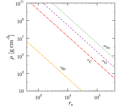
Figure 1: $\rho$–$r_{\mathrm{s}}$ relationship for several ion species.

We have performed extensive PIMC simulations of body-centered cubic (bcc) Coulomb crystals in periodic boundary conditions with $N=250$ ions in the density range relevant for astrophysical applications, $500\leq r_{\mathrm{s}}\leq 120000$, and for temperatures from the crystallization, parameterized approximately by the condition $\Gamma=175$ (see Sec. 7 for update), down to $T=T_{\mathrm{p}}/30$. In this case, $r_{\mathrm{s}}=a_{\mathrm{i}}/a_{\rm B}$, $a_{\rm B}=\hbar^{2}/(m_{\mathrm{i}}Z_{\mathrm{i}}^{2}e^{2})$ is the ion Bohr radius, $T_{\mathrm{p}}=\hbar\sqrt{4\pi n_{\mathrm{i}}Z_{\mathrm{i}}^{2}e^{2}/m_{\mathrm{i}}}$ is the ion plasma temperature, and $m_{\mathrm{i}}$ is the ion mass. Since $r_{\mathrm{s}}$ does not depend on temperature, it determines uniquely density $\rho$ for a specified composition. In Fig. 1, we show the relationship between the mass density and $r_{\mathrm{s}}$ for several nuclei typical of the WD interior.

The general method of calculations followed that described in Paper II for the liquid phase of the same system. Specifically, we adopt the so-called primitive approximation (e.g. Ceperley, 1995), in which the crystal energy,

$$\langle{\cal H}\rangle=\frac{{\rm Tr}\left[{\cal H}e^{-\beta{\cal H}}\right]}{{\rm Tr}\left[e^{-\beta{\cal H}}\right]}~{},$$ (1)

where ${\cal H}$ is the system Hamiltonian and $\beta=1/T$ is the imaginary time, can be expressed as

$$\langle{\cal H}\rangle=\int{\rm d}\sigma\pi(\sigma)H({\cal R}_{m})~{}.$$ (2)

In this case, $\sigma=\left\{{\cal R}_{1},{\cal R}_{2},\ldots,{\cal R}_{M}={\cal R}_{0}\right\}$ is the $3NM$-dimensional domain of quantum numbers, i.e. coordinates of $N$ ions in $M$ basis states of the coordinate representation. A basis state ${\cal R}_{l}$ ($l=1,2,\ldots,M$) is specified by cartesian coordinates of all $N$ ions: ${\cal R}_{l}=\left\{{\bm{R}}^{(l)}_{1},{\bm{R}}^{(l)}_{2},\ldots,{\bm{R}}^{(l)}_{N}\right\}$. $M$ is a positive integer, which, in this formulation, is called the total number of imaginary time slices. Equivalently, $\sigma$ is the domain of coordinates of $N$ classic ring polymers, each with $M$ beads.

Furthermore,

$$\pi(\sigma) = \frac{1}{Z}\exp{\left[-\sum_{l=1}^{M}S_{l}\right]}~{},$$ (3)

$$e^{-S_{l}} = \frac{1}{(4\pi\lambda\tau)^{3N/2}}\exp{\left[-\frac{({\cal R}_{l}-{\cal R}_{l-1})^{2}}{4\lambda\tau}-\tau V({\cal R}_{l})\right]}~{},$$

where $Z$ is the partition function, $\lambda=\hbar^{2}/(2m_{\rm i})$, $\tau=\beta/M$, and $V({\cal R})$ is the crystal potential energy, when ion coordinates are equal to ${\cal R}$. Finally, $H({\cal R}_{m})$ is the energy estimator. In this work, we use the thermodynamic energy estimator given, e.g. by equation (6.7) of Ceperley (1995). Possible values of $m$, to which the results should be insensitive, are $1,2,\ldots,M$.

Since $\pi(\sigma)$ is strictly positive and normalized to 1, it is natural to interpret it as a probability distribution, and the task of finding $\langle{\cal H}\rangle$ reduces to averaging the energy estimator with it. This can be done by sampling with the aid of the Metropolis algorithm. We attempt two move types: single bead moves and whole polymer moves.

Unlike in the liquid, the harmonic lattice thermodynamics of the crystal is well known (Paper I). Hence, it has been decided to separate out the anharmonic contribution to the energy. Since anharmonic energy is a subdominant contribution (it is smaller than the electrostatic, harmonic thermal and harmonic zero-point energies), this required an improved precision of numerical computations as compared to the liquid. The extra precision was achieved by performing several times longer PIMC runs and having multiple PIMC runs at fixed physical conditions (i.e. temperature and density or $r_{\mathrm{s}}$ and $\Gamma$), characterized by different random sequences and imaginary time slices $m$, at which the energy estimator was applied. Overall, the typical error bars for the present anharmonic energy calculations are estimated to be about 5 times smaller than the error bars of the liquid energy calculations in Paper II.

The energy estimates from multiple runs at a given temperature, density, and a total number $M$ of imaginary time slices (or a number of beads in a ring polymer representing a quantum ion) were averaged over the runs. Then, the energy of a harmonic crystal was subtracted from it. The harmonic crystal energy was calculated for the bcc lattice with periodic boundary conditions and the same $N$ and $M$ as in the PIMC simulation (see Appendix A for details). This allowed us to prevent a contamination of calculated anharmonic energies by relatively large finite-size corrections to the harmonic energy.

A detailed numerical analysis at 5 values of $M$ and several $(r_{\mathrm{s}},\Gamma)$ pairs has shown that the anharmonic energy estimates depended on $M$ as $c(r_{\mathrm{s}},\Gamma)-a(r_{\mathrm{s}},\Gamma)/M^{2}$, which is the same as the $M$-dependence of the harmonic energy [cf. equation (49)]. Having established the quadratic dependence on $1/M$, the data at all the other physical points were obtained at just two different $M$ and these data were directly used in the fitting procedure.

Since $N$-dependence is not studied quantitatively in this work (under assumption that $N=250$ is large enough for this dependence to saturate; see also a discussion of $N$-dependence in Sec. 3), the fitted energy is treated as the thermodynamic limit of the anharmonic energy. Combined with the well-known thermodynamic limit of the harmonic energy (Paper I) and with the Madelung energy, it represents our final estimate for the ion energy of the crystal.

3 Analytic expression for the anharmonic crystal energy

The ion energy (per ion) reads

$$U=\frac{\partial F\theta}{\partial\theta}=U_{\mathrm{M}}+U_{\mathrm{h}}+U_{\mathrm{ah}}~{},$$ (4)

where $F$ is the Helmholtz free energy per ion, $\theta\equiv T_{\mathrm{p}}/T=\Gamma\sqrt{3/r_{\mathrm{s}}}$, indices ‘M’, ‘h’, and ‘ah’ stand for Madelung (static perfect lattice), harmonic, and anharmonic contributions, respectively; see Paper I for analytic expressions for the first and second terms.

The numerical anharmonic contribution to the energy, $U_{\mathrm{ah}}$, can be approximated by a series over anharmonic corrections

$$\mathfrak{u}_{\rm ah}\equiv\frac{U_{\mathrm{ah}}a_{\mathrm{i}}}{Z^{2}e^{2}}=\frac{A^{U}_{1}(\theta)}{\Gamma^{2}_{\mathrm{q}}}+\frac{A^{U}_{2}(\theta)}{\Gamma^{3}_{\mathrm{q}}}+\frac{A^{U}_{3}(\theta)}{\Gamma^{4}_{\mathrm{q}}}~{},$$ (5)

where $\Gamma_{\mathrm{q}}\equiv Z^{2}e^{2}/(a_{\mathrm{i}}T_{\mathrm{p}})=\sqrt{r_{\mathrm{s}}/3}$ and

$$A^{U}_{1}(\theta) = -\frac{A_{11}}{\theta^{2}}\frac{3A_{12}\theta^{2}+1}{\left(1+A_{12}\,\theta^{2}\right)^{2}}$$

$$- \frac{A_{13}}{\theta^{2}}\frac{3A_{14}\theta^{2}+1}{\left(1+A_{14}\,\theta^{2}\right)^{2}}+A_{\mathrm{1q}}~{},$$

$$A^{U}_{2}(\theta) = \frac{A_{\mathrm{2cl}}}{\theta^{3}}\,\frac{2-A_{21}\,\theta^{4}}{2\,\left(1+A_{21}\,\theta^{4}\right)^{1/4}}~{},$$ (7)

$$A^{U}_{3}(\theta) = \frac{A_{\mathrm{3cl}}}{\theta^{4}}+A_{\mathrm{3q}}.$$ (8)

In this case, indices ‘cl’ and ‘q’ indicate coefficients, determining classic and quantum asymptotes discussed below. Moreover, the following set of constraints is assumed to be satisfied

$$A_{13} = -A_{\mathrm{1cl}}-A_{11}~{},$$ (9)

$$A_{14}A_{13} = A_{\mathrm{1q}}-A_{11}A_{12}~{},$$ (10)

$$A_{21}^{3/4} = -\frac{2A_{\mathrm{2q}}}{A_{\mathrm{2cl}}}~{},$$ (11)

where the quantities on the left-hand sides are calculated rather than fitted. Equations (10) and (11) ensure that the anharmonic energy has the same, $\propto T^{4}$, asymptote as the harmonic energy at very low temperatures ($\theta\gg 1$). This assumption is unmistakably supported by the PIMC data at $\theta\leq 30$. Inclusion of terms of higher-order in anharmonism is likely required to extend the fit to extremely high densities, $r_{\mathrm{s}}<500$. This is beyond the scope of the present work, because, as discussed in Sec. 7, such densities are unrealistic (see also Fig. 1).

In general, the anharmonic energy can be split into two parts, the zero-point and the thermal contributions. Both are contained in equation (5). The thermal part of the anharmonic energy is positive. For a classic crystal, only thermal contribution to the anharmonic energy exists, and it was studied earlier semi-analytically (Albers & Gubernatis, 1986; Dubin, 1990), by classic Monte Carlo (Stringfellow et al. 1990), and by molecular dynamics methods (Farouki & Hamaguchi, 1993). According to the results of these studies, the classic anharmonic energy can be presented in the form of an expansion over $\Gamma$

$$\frac{U_{\mathrm{ah,cl}}}{T}=\frac{A_{\mathrm{1cl}}}{\Gamma}+\frac{A_{\mathrm{2cl}}}{\Gamma^{2}}+\frac{A_{\mathrm{3cl}}}{\Gamma^{3}}~{}.$$ (12)

The functional form of equation (12) is consistent with our data at quasiclassic conditions and is reproduced by equation (5) in the limit $\theta\to 0$ by construction.

The literature values of the classic anharmonic coefficients in equation (12) have some scatter (cf. Dubin, 1990; Farouki & Hamaguchi, 1993). In particular, Farouki & Hamaguchi (1993) suggest several sets of anharmonic coefficients, depending on $\Gamma$ range and the number of anharmonic terms in their fit to the numerical data. The coefficients vary quite a bit from set to set (for instance, $A_{\mathrm{1cl}}$ varies from 5.98 to 10.9) with little effect on the fit accuracy. The set from line 1 of table 5 in this reference: $A^{\rm astro}_{\mathrm{1cl}}=10.9$, $A^{\rm astro}_{\mathrm{2cl}}=247$, and $A^{\rm astro}_{\mathrm{3cl}}=1.765\times 10^{5}$ is widely employed in astrophysics (e.g. Potekhin & Chabrier, 2010). On the other hand, in plasma community (e.g. Dubin & O’Neil, 1999; Khrapak & Khrapak, 2016), the set suggested by Dubin (1990) is in frequent use: $A^{\rm plasma}_{\mathrm{1cl}}=10.84$, $A^{\rm plasma}_{\mathrm{2cl}}=352.8$, and $A^{\rm plasma}_{\mathrm{3cl}}=1.794\times 10^{5}$.

Our PIMC data can be fitted quite satisfactorily with the ‘cl’ fit coefficients in equations (5)–(11) fixed to the “astrophysical” values above, but if they are fixed to the “plasma physics” values, the fit (5) becomes noticeably worse (rms error increases by $\sim 40\%$). At the same time, the best fit to our data corresponds to a bit different set of values: $A_{\mathrm{1cl}}=10.2$, $A_{\mathrm{2cl}}=248$, and $A_{\mathrm{3cl}}=2.03\times 10^{5}$ (cf. Tab. 1), which lie within the scatter of published classic anharmonic coefficients.

$A_{\mathrm{1cl}}$	$10.2$
$A_{\mathrm{2cl}}$	$248$
$A_{\mathrm{3cl}}$	$2.03\cdot 10^{5}$
$A_{1\mathrm{q}}$	$-0.62/6$
$A_{2\mathrm{q}}$	$-0.56$
$A_{3\mathrm{q}}$	$2.35$
$A_{11}$	$-10$
$A_{12}$	$6\cdot 10^{-3}$
$B_{1}$	$0.13$
$B_{2}$	$4\cdot 10^{-4}$
rms err	$5\times 10^{-6}$
max err	$1.5\times 10^{-5}$

Table 1: The fitting parameters

As shown by Carr, Coldwell-Horsfall & Fein (1961), Ceperley (1978), and Albers & Gubernatis (1986), the anharmonic zero-point energy can be expanded in powers of $r_{\mathrm{s}}^{-1/2}$, with the lowest-order term being negative and inversely proportional to $r_{\mathrm{s}}^{2}$. Our numerical data and fit reproduce this behavior with a slightly different coefficient. Namely, we get $6A_{\mathrm{1q}}=-0.62$, whereas Carr et al. (1961) and Ceperley (1978) had, for the same quantity, $-0.73$, while Albers & Gubernatis (1986) reported $-0.703$. As above, the PIMC data can be fitted satisfactorily with the values for $6A_{\mathrm{1q}}$ reported by previous authors, whereas $-0.62$ is our best fit value. On top of that, our fit expression contains higher-order terms of the anharmonic zero-point energy expansion.

Overall, our fit has 8 numerical parameters in equations (3)–(8), which are listed in Tab. 1 with minimum required number of digits along with the rms and maximum fit errors. Two additional fitting parameters, $B_{1}$ and $B_{2}$, describe the dependence of the finite-$M$ correction coefficient $a(r_{\mathrm{s}},\Gamma)$ on $r_{\mathrm{s}}$ and $\Gamma$ as follows

$$a(r_{\mathrm{s}},\Gamma)=3\,B_{1}\frac{\Gamma^{2}}{r_{\mathrm{s}}^{2}}\,\left(1+B_{2}\,\theta^{2}\right)^{-1}~{}.$$ (13)

This coefficient is not needed for astrophysical applications, but may be usefull for subsequent PIMC studies.

At intermediate temperatures, where neither classic nor quantum asymptotes apply, our results, for the first time, provide the detailed first-principle temperature and density dependence of the true quantum anharmonic energy and thermodynamics of a Coulomb crystal.

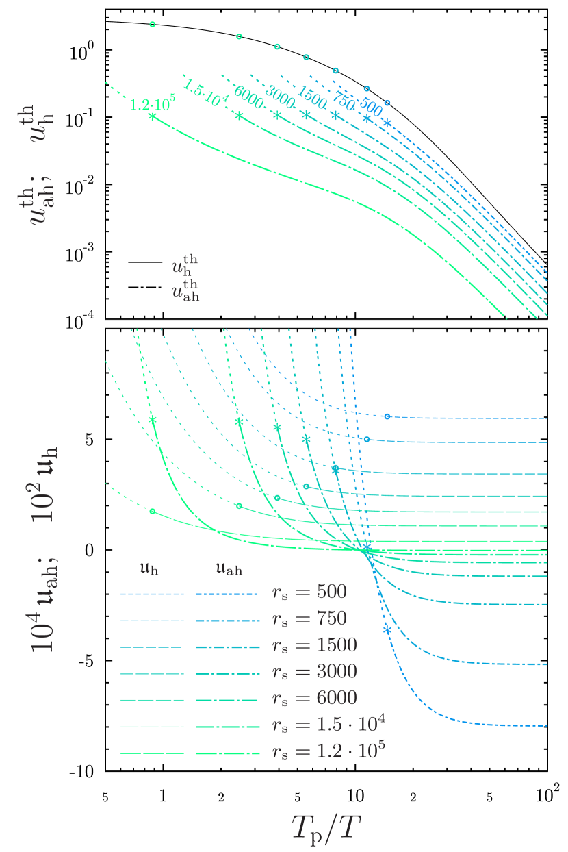
Figure 2: Bottom panel: thin dashed and thick dot-dashed curves show harmonic ($\times 10^{2}$) and anharmonic ($\times 10^{4}$) contributions to the one-component quantum ion crystal energy in units of $Z^{2}e^{2}/a_{\mathrm{i}}$ [$\mathfrak{u}_{\rm h,ah}\equiv a_{\mathrm{i}}U_{\rm h,ah}/(Z^{2}e^{2})$]. Different density of dashes corresponds to different $r_{\mathrm{s}}$ values. Symbols indicate melting temperatures at respective $r_{\mathrm{s}}$. Dotted portions of the curves describe a superheated crystal. Top panel: thermal harmonic (thin, solid, same for all $r_{\mathrm{s}}$) and anharmonic (thick, dot-dashed) contributions to the energy in units of $T$, without multiplication by extra powers of $10$ ($u_{\rm h,ah}\equiv U_{\rm h,ah}/T$).

In Fig. 2, bottom panel, we plot harmonic (multiplied by $10^{2}$, thin, dashed) and anharmonic (multiplied by $10^{4}$, thick, dot-dashed) crystal energies in units of $Z^{2}e^{2}/a_{\mathrm{i}}$ as functions of $T_{\rm p}/T$ for several values of $r_{\mathrm{s}}$ in the range $500\leq r_{\mathrm{s}}\leq 120000$. Symbols indicate melting temperatures with account of the $\Gamma_{\rm m}(r_{\mathrm{s}})$ dependence established in Sec. 7. At higher temperatures (lower $T_{\rm p}/T$), the system is assumed to be in a superheated crystal state (dotted portions of the curves). The anharmonic energies are given by the present fit, while harmonic energies are taken from Paper I.

Top panel shows only the thermal (‘th’) harmonic and anharmonic contributions to the energy in units of $T$ and without multiplication by extra numerical factors. If expressed in units of temperature, harmonic contributions to the energy (as well as to the Helmholtz free energy, cf. Fig.3) are independent of $r_{\mathrm{s}}$.

Since the total anharmonic energy is a sum of the (negative) zero-point and (positive) thermal contributions, at any density, there is a temperature where the total anharmonic energy is zero. For $r_{\mathrm{s}}>600$, it takes place at $T=(10-12)T_{\mathrm{p}}$. Even more peculiar is the fact that there exists a density ($r_{\mathrm{s}}\approx 735$), at which the total anharmonic energy is zero at melting!

Let us note in passing, that for $N=250$ particles, Dubin (1990) has found analytically $A_{\mathrm{1cl}}=10.036$, which is closer to our best fit value. This represents an 8% deviation from the (analytic) thermodynamic limit reported by the same author, $A^{\rm plasma}_{\mathrm{1cl}}=10.84$, due to a finite-$N$ effect at $N=250$. Strong $N$-dependence of the classic thermal anharmonic energy has been seen by Albers & Gubernatis (1986), however, these authors have also observed unwelcome dependence on the mesh type and oscillating $N$-dependence (cf. their Figs. 1 and 2).

In general, 8% seems to be a surprisingly large finite-$N$ correction to an energy at $N=250$. Naively, one expects the correction to be $\sim 1/N\sim 0.4\%$. In fact, this is what we find for the finite-$N$ correction to the harmonic zero-point energy and to the harmonic classic entropy, determined by the phonon frequency moments $\langle\omega/\omega_{\rm p}\rangle$ and $\langle\ln{(\omega/\omega_{\rm p})}\rangle$, respectively (see Fig. 15 in the Appendix A; $\omega_{\rm p}=T_{\rm p}/\hbar$ is the ion plasma frequency). Classic thermal harmonic energy has $N$-correction of the same, $1/N$, order [e.g. equation (18) of Dubin (1990)]. Note also an $\approx 1/N$ difference between our best fit $A_{\mathrm{2cl}}$ and $A^{\rm astro}_{\mathrm{2cl}}$, even though the latter coefficient is obtained from a simulation with $N=1024$ particles. Finally, Fig. 2 of Albers & Gubernatis (1986) seems to indicate that the lowest-order anharmonic zero-point energy does not demonstrate strong $N$-dependence either.

On the other hand, the formulae derived by Dubin (1990) for $A_{\mathrm{1cl}}$ have phonon frequencies in the denominator, whereas the phonon frequency moment $\langle\omega_{\rm p}^{2}/\omega^{2}\rangle$ does have an $N$-correction of a similar order (cf. Fig. 15). Thus, summarizing the discussion, we should warn the reader that our fit for the anharmonic energy may be affected by finite-size effects especially noticeable (at the level of $\sim 8\%$) in the lowest-order anharmonic classic term. It would require significantly more computer resources to get rid of said effects in a first-principle PIMC simulation.

4 Thermodynamics of the crystal

The ion Helmholtz free energy (per ion) can be written as

$$F=F_{\mathrm{M}}+F_{\mathrm{h}}+F_{\mathrm{ah}}~{},$$ (14)

where the Madelung, harmonic, and anharmonic terms can be obtained by thermodynamic integration from the respective terms in equation (4). In particular, the anharmonic term also takes the form of a series over anharmonic corrections

$$\mathfrak{f}_{\rm ah}\equiv\frac{F_{\rm ah}a_{\mathrm{i}}}{Z^{2}e^{2}}=\frac{A^{F}_{1}(\theta)}{\Gamma^{2}_{\mathrm{q}}}+\frac{A^{F}_{2}(\theta)}{\Gamma^{3}_{\mathrm{q}}}+\frac{A^{F}_{3}(\theta)}{\Gamma^{4}_{\mathrm{q}}}~{}.$$ (15)

The respective functions are

$$A^{F}_{1}(\theta) = \frac{A_{11}}{\theta^{2}}\frac{1}{1+A_{12}\,\theta^{2}}+\frac{A_{13}}{\theta^{2}}\frac{1}{1+A_{14}\,\theta^{2}}+A_{\mathrm{1q}}~{},$$ (16)

$$A^{F}_{2}(\theta) = -\frac{A_{\mathrm{2cl}}}{2\theta^{3}}\,\left(1+A_{21}\theta^{4}\right)^{3/4}~{},$$ (17)

$$A^{F}_{3}(\theta) = -\frac{A_{\mathrm{3cl}}}{3\theta^{4}}+A_{\mathrm{3q}}~{}.$$ (18)

Once the free energy is known, it is straightforward to derive all the other thermodynamic functions. For instance, the ion entropy $S$ (per ion) is

$$S=-\left.\frac{\partial F}{\partial T}\right|_{V,N}=\frac{\theta^{2}}{T_{\rm p}}\,\frac{\partial F}{\partial\theta}=\frac{U-F}{T}=S_{\mathrm{h}}+S_{\mathrm{ah}},$$ (19)

where

$$S_{\mathrm{ah}}=\frac{\theta^{2}}{T_{\rm p}}\,\frac{\partial F_{\mathrm{ah}}}{\partial\theta}=\frac{A^{S}_{1}(\theta)}{\Gamma_{\mathrm{q}}}+\frac{A^{S}_{2}(\theta)}{\Gamma^{2}_{\mathrm{q}}}+\frac{A^{S}_{3}(\theta)}{\Gamma^{3}_{\mathrm{q}}}.$$ (20)

The analytic form of the coefficients is:

$$A^{S}_{1}(\theta) = -\frac{2A_{11}}{\theta}\frac{2\,A_{12}\theta^{2}+1}{\left(1+A_{12}\,\theta^{2}\right)^{2}}$$ (21)

$$- \frac{2A_{13}}{\theta}\frac{2\,A_{14}\theta^{2}+1}{\left(1+A_{14}\,\theta^{2}\right)^{2}}~{},$$

$$A^{S}_{2}(\theta) = \frac{3\,A_{\mathrm{2cl}}}{2\,\theta^{2}}\frac{1}{\left(1+A_{21}\,\theta^{4}\right)^{1/4}}~{},$$ (22)

$$A^{S}_{3}(\theta) = \frac{4\,A_{\mathrm{3cl}}}{3\theta^{3}}~{}.$$ (23)

Similarly, the ion specific heat $C$ (per ion) reads

$$C=\left.\frac{\partial S}{\partial\ln T}\right|_{V,N}=-\theta\frac{\partial S}{\partial\theta}=C_{\mathrm{h}}+C_{\mathrm{ah}},$$ (24)

where

$$C_{\mathrm{ah}}=-\theta\frac{\partial S_{\mathrm{ah}}}{\partial\theta}=\frac{A^{C}_{1}(\theta)}{\Gamma_{\mathrm{q}}}+\frac{A^{C}_{2}(\theta)}{\Gamma^{2}_{\mathrm{q}}}+\frac{A^{C}_{3}(\theta)}{\Gamma^{3}_{\mathrm{q}}}.$$ (25)

The analytic form of the coefficients is:

$$A^{C}_{1}(\theta) = -\frac{2\,A_{11}}{\theta}\,\frac{6\,A_{12}^{2}\theta^{4}+3\,A_{12}\,\theta^{2}+1}{\left(1+A_{12}\theta^{2}\right)^{3}}$$

$$- \frac{2\,A_{13}}{\theta}\,\frac{6\,A_{14}^{2}\theta^{4}+3\,A_{14}\,\theta^{2}+1}{\left(1+A_{14}\theta^{2}\right)^{3}}~{},$$

$$A^{C}_{2}(\theta) = \frac{3\,A_{\mathrm{2cl}}}{2\,\theta^{2}}\frac{2+3\,A_{21}\theta^{4}}{\left(1+A_{21}\,\theta^{4}\right)^{5/4}}~{},$$ (27)

$$A^{C}_{3}(\theta) = 4\,\frac{A_{\mathrm{3cl}}}{\theta^{3}}~{}.$$ (28)

Finally, analytic formulae for the ion pressure read:

$$P = -N\left(\frac{\partial F}{\partial V}\right)_{T}=P_{\mathrm{M}}+P_{\rm h}+P_{\rm ah}~{},$$

$$\frac{P_{\rm ah}a_{\mathrm{i}}}{n_{\mathrm{i}}Z^{2}e^{2}} = \frac{S_{\rm ah}}{2\Gamma}+\frac{2A^{F}_{1}(\theta)}{3\Gamma^{2}_{\mathrm{q}}}+\frac{5A^{F}_{2}(\theta)}{6\Gamma^{3}_{\mathrm{q}}}+\frac{A^{F}_{3}(\theta)}{\Gamma^{4}_{\mathrm{q}}}~{}.$$ (29)

$P_{\mathrm{M}}=n_{\mathrm{i}}U_{\mathrm{M}}/3$ is the (negative) electrostatic or Madelung contribution to the pressure.

Let us remind, that the thermodynamic functions $F_{\mathrm{h}}$, $S_{\mathrm{h}}$, $C_{\mathrm{h}}$, and $P_{\mathrm{h}}$ can be easily derived from the harmonic lattice thermodynamics fits of Paper I.

In Figs. 3 and 4, we show crystal ion Helmholtz free-energy and ion specific heat as functions of $T_{\rm p}/T$ for several $r_{\mathrm{s}}$ values. Thin dashed curves in the bottom panel of Fig. 3 display harmonic contributions. Thick dot-dashed curves are anharmonic quantities based on the present fit. Top panel shows absolute values of the thermal contributions to the free energy, which are actually negative. The harmonic contribution, drawn by a thin solid curve, is insensitive to $r_{\mathrm{s}}$. The Helmholtz free energy will be discussed further in Sec. 7.

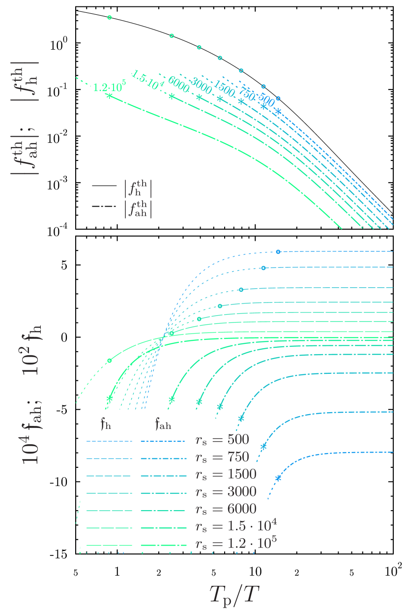
Figure 3: Same as in Fig. 2 but for the crystal ion Helmholtz free energy [$\mathfrak{f}_{\rm h,ah}\equiv a_{\mathrm{i}}F_{\rm h,ah}/(Z^{2}e^{2})$, $f_{\rm h,ah}\equiv F_{\rm h,ah}/T$]. Top panel shows absolute values of (negative) thermal contribultions to the free energy.

In Fig. 4, the harmonic contribution to the ion specific heat is shown by a thin solid line, and it is also the same for all $r_{\mathrm{s}}$. In the quantum limit of low temperatures, the anharmonic specific heat (thick, dot-dashed) exhibits the same $T^{3}$ dependence as predicted by the Debye law for the harmonic contribution. At high temperatures, the temperature dependence of the anharmonic specific heat is more complex. It does not saturate and increases rather rapidly with temperature increase, even exceeding the harmonic contribution in the superheated phase.

In the normal crystal phase, the anharmonic specific heat is always smaller than the harmonic one, but its relative importance grows, as the system becomes denser ($r_{\mathrm{s}}$ decreases). For instance, at $r_{\mathrm{s}}=120000$, the anharmonic specific heat is about 30 times smaller than the harmonic one in the quantum asymptote regime, becomes almost 100 times smaller at $\theta\sim 5$, and is only 10 times smaller at melting. By contrast, at $r_{\mathrm{s}}=600$, the anharmonic contribution is only about two times smaller than the harmonic one in the $\propto T^{3}$ regime, and the ratio reaches maximum of about 3 at $T_{\mathrm{p}}\sim 20T$.

It is worth noting, that the anharmonic specific heat at the melting point is $\sim 0.3$, being almost independent of $r_{\mathrm{s}}$.

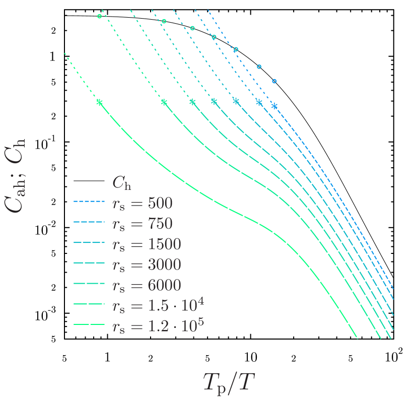
Figure 4: Harmonic (thin, solid, one curve for all $r_{\mathrm{s}}$) and anharmonic (thick, dashed) contributions to the specific heat of the one-component quantum ion crystal. Symbols indicate melting temperatures. Dotted portions of the curves assume a superheated crystal.

5 Comparison with earlier work

Let us compare the first-principle quantum thermodynamics of a one-component ion crystal developed above with several earlier works.

First-principle PIMC calculations of the Coulomb crystal energy have been performed earlier by Iyetomi et al. (1993) and Jones & Ceperley (1996). A comparison of the anharmonic energy, reported by Iyetomi et al. (1993) and shown in their Fig. 6, reveals an agreement with our fit at nearly classic temperatures $\theta\lesssim 4$. Deeper into the quantum domain, their points deviate from our fit at all $\Gamma$, and the discrepancy steadily grows with increase of $\Gamma$. In the ultra-quantum regime, $50\lesssim r_{\mathrm{s}}\lesssim 500$, dominated by the zero-point asymptote, our fit and their data points are again in a rough agreement with each other except at $\Gamma=1000$, where their data is poor. Unfortunately, we do not have a way of identifying the source of the disagreement at intermediate $\theta$. What is clear is that our approach employs more particles, MC iterations, beads, contains an accurate subtraction of the harmonic energy at a finite $N$, and does not use any analogs of a cumulant expansion. Besides, their prediction for the anharmonic entropy (Fig. 7 of Iyetomi et al., 1993) looks implausible with a value, greatly exceeding the harmonic contribution at $T\ll T_{\mathrm{p}}$, and a minimum at intermediate $\theta$.

Jones & Ceperley (1996) have presented PIMC calculations with $N=54$ ions of the bcc solid phase energy (harmonic plus anharmonic) at $r_{\mathrm{s}}=200$, $400$, $625$, and $1200$. We assume that the data points shown in their Fig. 2 include the finite-$N$ correction described by their equation (1). These data points do not agree with our anharmonic fit combined with the harmonic energy taken in the thermodynamic limit (from Paper I). However, if one removes the finite-$N$ correction from the data points in Fig. 2 of Jones & Ceperley (1996), the raw PIMC data obtained in this way agree reasonably well with our anharmonic fit combined with the harmonic energy of a lattice with $N=54$ ions (see Sec. A.2 for details). We thus conclude that the data in Fig. 2 of Jones & Ceperley (1996) is likely compromised by inaccurate treatment of finite-size effects in a harmonic lattice.

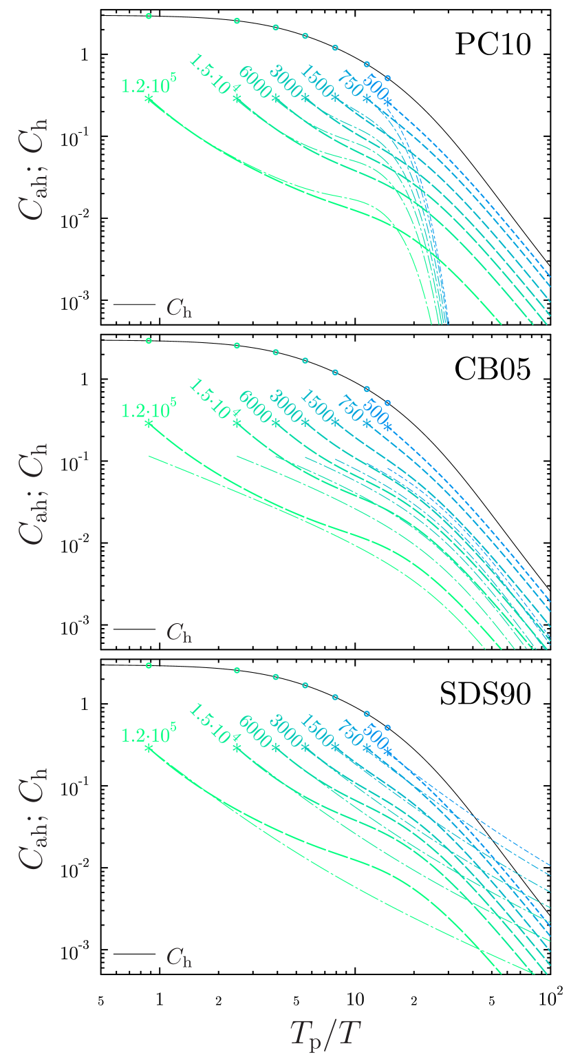
Figure 5: Various results for ion crystal specific heat. Thin solid lines display the harmonic contribution $C_{\mathrm{h}}$ from Paper I (same for all $r_{\mathrm{s}}$). Dashes show the anharmonic contributions calculated in this work (and already shown in Fig. 4) at $r_{\mathrm{s}}$ values indicated near the curves. Thin dot-dashed lines represent previously available parametrizations: Potekhin & Chabrier (2010) (top panel), Chugunov & Baiko (2005) (middle panel), and Stringfellow et al. (1990) (bottom panel).

Thus, the most obvious advantage of our calculations over those of Iyetomi et al. (1993) and Jones & Ceperley (1996) is their very detailed nature and superior accuracy, which allowed us to develop a highly constrained fit. The fit can be integrated and differentiated to produce reliable thermodynamics free of unphysical artefacts in the astrophysically meaningful density range.

In Fig. 5, using the specific heat as an example, we illustrate the difference between our PIMC calculations of the ion crystal thermodynamics and several earlier parametrizations available in the literature. For reference, by thin solid line, we plot the harmonic specific heat from Paper I (same as in Fig. 4). This contribution is a universal function of $\theta$, i.e. it is the same for all densities at fixed $\theta$. Dashes (same as in Fig. 4) show the anharmonic contribution to the specific heat calculated in this work at the $r_{\mathrm{s}}$ values indicated near the curves.

Thin dot-dashed lines in the top panel display widely used interpolation of the anharmonic contribution to the specific heat suggested by Potekhin & Chabrier (2010). It assumes an exponential suppression of the thermal anharmonic energy and specific heat in quantum regime, which clearly disagrees with our data and fit.

Furthermore, for anharmonic correction to the zero-point energy, this interpolation uses only the lowest-order anharmonic term calculated by Carr et al. (1961), Ceperley (1978), and Albers & Gubernatis (1986). According to our simulations, this is not accurate enough at $r_{\mathrm{s}}\lesssim 1500$.

Table 2: PIMC energies in the liquid phase at $r_{\mathrm{s}}=500$

$\Gamma$	90	101	112	123	134	145	156	167	178
$(U-U_{\rm M})/T$	6.344	6.951	7.565	8.185	8.811	9.438	10.072	10.707	11.343

Chugunov & Baiko (2005) have analyzed quantum anharmonic corrections to the Coulomb crystal thermodynamics based on the harmonic pair correlation function. The main aim of that paper was to obtain an estimate of the quantum anharmonic correction to the crystal specific heat. The lowest-order anharmonic correction at arbitrary strength of quantum effects was formally included, but the very approach was manifestly approximate. For instance, the zero-point properties, obtained in Chugunov & Baiko (2005), were completely inaccurate. Nevertheless, the anharmonic crystal specific heat, shown by thin dot-dashed curves in the middle panel of Fig. 5, is seen to be in a rough qualitative agreement with the first-principle (dashed) curves.

Thin dot-dashed lines in the bottom panel of Fig. 5 represent the specific heat, calculated by differentiation of the anharmonic energy given by fits in Stringfellow et al. (1990). This approach seems to be still applied as microphysics input in WD cooling theory (e.g. Segretain et al.,, 1994; Salaris et al.,, 2021), even though it completely ignores the ion quantum effects for the anharmonic term. These effects were not considered by Stringfellow et al. (1990), whose work was based on purely classic Monte Carlo. As a result, the anharmonic specific heat is strongly overestimated at low temperatures ($T\ll T_{\mathrm{p}}$), has a wrong asymptote, and can even exceed the harmonic contribution, thus corrupting modelling of the Debye cooling stage.

Table 3: Numerical results for $(U-U_{\rm M})/T$ in the liquid phase near melting

	$r_{\rm s}$
$\Gamma$	500	600	750	950	1200	1500
178	11.343	10.508	9.593	8.736	7.995	7.373
181	11.517	10.668	9.733	8.860	8.104	7.472
184	11.692	10.827	9.874	8.985
187	11.866	10.984	10.015		8.324
190	12.040	11.143	10.156

Finally, let us mention that Hansen & Vieillefosse (1975) have analyzed the Wigner-Kirkwood expansion of the free energy of the OCP up to the terms of order $\hbar^{4}$. The lowest-order, $\propto\hbar^{2}$, correction does not depend on the OCP state (liquid or crystal). In the solid phase, it is a part of the harmonic energy (e.g. Paper I). Moreover, the leading $\hbar^{4}$-term in equation (7) of Hansen & Vieillefosse (1975) (which is independent of $\Gamma$) almost coincides (the relative difference is just $\sim 10^{-3}$) with the respective term in the Taylor series for the harmonic energy. To verify this, we have used the harmonic energy fit from Paper I.

Thus, the remaining terms in equation (7) of Hansen & Vieillefosse (1975) ($\propto 1/\Gamma$ and $\propto 1/\Gamma^{2}$) must correspond to quantum corrections to the anharmonic energy. We have compared these terms with the Taylor expansion of our anharmonic coefficients, equations (3) and (7), at $\theta\rightarrow 0$, and have found a disagreement by a factor of a few. The most likely reason for the discrepancy is the replacement by Hansen & Vieillefosse (1975) of the three-body correlation function by a static-lattice value in their final formula for the $K$-term (see Hansen & Vieillefosse 1975 for details). Such a replacement removes any $\Gamma$-dependence from the $K$-term and can make a quantum correction to the anharmonic energy inaccurate.

Note, that already at $\theta\sim 1$, the next order, $\propto\hbar^{6}$, quantum corrections are required, which renders the entire WK expansion not very useful (cf. a similar situation in the liquid as discussed in Jones & Ceperley, 1996, and in Paper II).

6 Liquid phase thermodynamics update

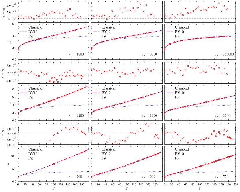
Figure 6: PIMC energies in the liquid vs. $\Gamma$ (crosses) for several values of $r_{\mathrm{s}}$. Thin solid lines represent the fit (30) with $u_{\rm q}$ given by equation (31), thick dashed lines are the Paper III fit, dotted lines display the right-hand side of equation (30) with $u_{\rm q}$ set to 0.

Once the crystal thermodynamics is constructed, it can be combined with liquid thermodynamics of Paper III to obtain a phase diagram of the strongly-coupled ion plasma at physically relevant densities and temperatures. Before doing this, we can take advantage of the fact, that calculations of the liquid energies were extended by one of us to $r_{\mathrm{s}}=500$ (Baiko, 2021, these energies are reported here in table 2). Besides that, we have performed new PIMC simulations in the liquid phase at the lower end of the $r_{\mathrm{s}}$ range, studied in this paper, in the vicinity of the crystallization, which occurs at $\Gamma>175$ (cf. Sec. 1). These energies are presented in table 3.

Table 4: Fit coefficients in equation (33)

$P_{1}$	$P_{2}$	$P_{3}$
$0.351$	$0.294$	$90$

Even though these new data points were in an acceptable agreement with the fit proposed in Paper III, it was clear that the numerical energies and the fit started diverging. This could have resulted in noticeable inaccuracies of thermodynamic quantities, especially those obtained by fit differentiation, in the vicinity of the phase transition and at $r_{\mathrm{s}}\sim 500$. We have therefore modified the fit of Paper III to improve the agreement with the new data in the liquid. [In addition, it has been noticed by Jermyn et al. (2021) that the fit of Paper III demonstrated unphysical behaviour in the practically unattainable region of very high densities, $r_{\mathrm{s}}\lesssim 300$. This behaviour is also corrected by the present fit modification.]

Let us remind, that the fit proposed in equation (4) of Paper III had the following form (note, that our $U$ is the energy per ion)

$$\frac{U}{T}=\frac{3}{2}+u_{\rm cl}(\Gamma)+u_{\rm q}~{},$$ (30)

where the first two terms on the right-hand side were the same as in the classic liquid (Potekhin & Chabrier, 2000), while the new term $u_{\rm q}$ was responsible for the ion quantum effects. To avoid a confusion, let us stress, that $u_{\rm cl}$ and $u_{\rm q}$ are normalized to the temperature, whereas $\mathfrak{u}_{\mathrm{ah}}$ from Sec. 3 is normalized to the typical Coulomb energy $Z_{\mathrm{i}}^{2}e^{2}/a_{\mathrm{i}}$.

In this work, we suggest an updated expression for $u_{\rm q}$:

$$u_{\rm q} = u_{1}+u_{2}+u_{3}~{},$$ (31)

$$u_{i} = \frac{\theta_{i}}{1-\exp{(-\theta_{i})}}-\frac{\theta_{i}}{2}-1~{}.$$ (32)

In this case, $\theta_{i}=C_{i}\theta$, $i=1,2,3$, the quantities $C_{1}$, $C_{2}$, and $C_{3}$ are given by

$$C_{1}=\frac{P_{1}r_{\mathrm{s}}}{P_{3}+r_{\mathrm{s}}}~{},~{}~{}~{}C_{2}=P_{2}~{},~{}~{}~{}C_{3}=\sqrt{1-C_{1}^{2}-C_{2}^{2}}~{},$$ (33)

and the coefficients $P_{1}$, $P_{2}$, and $P_{3}$ are summarized in table 4. By construction, equations (31)–(33) reproduce the lowest-order term of the Wigner-Kirkwood expansion.

It was observed in Paper III, on the basis of the data from Paper II (at $r_{\mathrm{s}}\geq 600$), that $u_{\rm q}$ depended only on $\theta$ and not on temperature and density (or any other two parameters, such as $\Gamma$ and $r_{\mathrm{s}}$ or $\theta$ and $r_{\mathrm{s}}$) separately. This was not expected from the very beginning but stemmed from the fitting procedure. To emphasize this fact, the term was denoted $u_{\rm q}(\eta)$ in Paper III ($\eta$ of Paper III is our $\theta/\sqrt{3}$). Calculations at $r_{\mathrm{s}}=500$ revealed a subtle departure from this behavior. It was found, that $u_{\rm q}$ was better described by a function of $\theta$ [cf. equation (32)] with coefficients $C_{1}$ and $C_{3}$ depending explicitly on $r_{\mathrm{s}}$. This means that the quantum correction becomes a function of two variables: $u_{\rm q}(\theta,r_{\mathrm{s}})$.

Accuracy of the new fit for $r_{\mathrm{s}}\gtrsim 1900$ is roughly the same as that of the Paper III fit, but, at $r_{\mathrm{s}}\lesssim 1900$, and especially at $r_{\mathrm{s}}=500$, the present formula fits the data better (cf. Fig. 6). Additionally, we do not notice any unwanted effects, if the present fit is applied in the region $r_{\mathrm{s}}<500$. More information on the properties of the new fit is given in Appendix B.

The new equation (31) for $u_{\rm q}$ results in a modification of quantum corrections to other ion thermodynamic functions and, in particular, to practical formulae (12)–(15) of Paper III describing them. Specifically, for the Helmholtz free energy (divided by $NT$), the last line of equation (12) of Paper III has to be replaced by $f_{\rm q}=f_{1}+f_{2}+f_{3}$, where

$$f_{i}=\ln{\left[\exp{(\theta_{i})}-1\right]}-\frac{\theta_{i}}{2}-\ln{\theta_{i}}~{}.$$ (34)

For the isochoric specific heat, the last line of equation (13) of Paper III has to be replaced by $c_{\rm q}=c_{1}+c_{2}+c_{3}$, where

$$c_{i}=\frac{\partial(Tu_{i})}{\partial T}=u_{i}-\theta_{i}\frac{{\rm d}u_{i}}{{\rm d}\theta_{i}}=\frac{\theta_{i}^{2}\exp{(\theta_{i})}}{[\exp{(\theta_{i})}-1]^{2}}-1~{}.$$ (35)

Ion pressure becomes

$$P=P_{\rm id}\left(1+\frac{1}{3}u_{\rm cl}+\frac{1}{2}u_{\rm q}-\frac{1}{3}\sum_{i=1}^{3}D_{i}u_{i}\right)~{},$$ (36)

where $P_{\rm id}=n_{\rm i}T$ is the ideal ion gas pressure, and $D_{i}={\rm d}\ln{C_{i}}/{\rm d}\ln{r_{\rm s}}$, so that

$$D_{1}=\frac{P_{3}}{P_{3}+r_{\rm s}}~{},~{}~{}~{}D_{2}=0~{},~{}~{}~{}D_{3}=-\frac{C_{1}^{2}}{C_{3}^{2}}\frac{P_{3}}{P_{3}+r_{\rm s}}~{}.$$ (37)

For the temperature derivative of the ion pressure (divided by the ion density), the last line of equation (14) of Paper III has to be replaced by

$$\frac{1}{2}c_{\rm q}-\frac{1}{3}\sum_{i=1}^{3}D_{i}c_{i}~{}.$$ (38)

Finally, for the density derivative of the ion pressure (divided by $T$), the last line of equation (15) of Paper III has to be replaced by

$$\frac{3}{4}u_{\rm q}-\frac{1}{4}c_{\rm q}-\frac{1}{2}\sum_{i=1}^{3}D_{i}\left(u_{i}-\frac{1}{3}c_{i}\right)+\frac{1}{9}\sum_{i=1}^{3}r_{\rm s}\frac{{\rm d}D_{i}}{{\rm d}r_{\rm s}}u_{i}~{}.$$ (39)

7 Thermodynamics across melting transition

In this Section, we use the newly available thermodynamic information to obtain the phase diagram of the strongly-coupled ion plasma at astrophysically relevant densities and temperatures, neglecting ion-electron and higher-order electron contributions as described in the Introduction. The previous attempts at constructing the OCP phase diagram included the work of Chabrier (1993), who used a quantum extension of the Lindemann criterion, and Jones & Ceperley (1996), who performed a PIMC study of the OCP. In both cases, the phase diagrams extended into the domain of very high densities, $r_{\mathrm{s}}\ll 500$, where ion OCP cannot exist due to rapid nuclear fusion reactions, which immediately change the composition and effectively increase $r_{\mathrm{s}}$ back to the range addressed in the present paper (e.g. Baiko, 2021, and references therein).

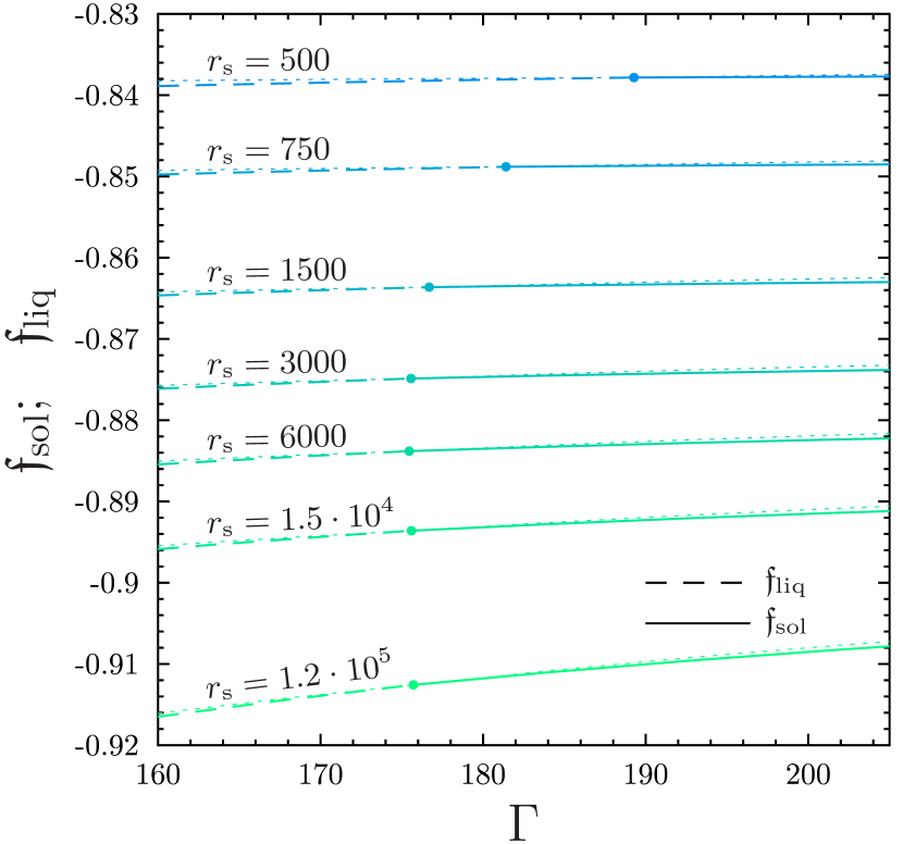
Figure 7: Crystal (solid) and liquid (dashed) Helmholtz free energies of the ion OCP [$\mathfrak{f}_{\rm sol,\,liq}\equiv a_{\mathrm{i}}F_{\rm solid,\,liquid}/(Z^{2}e^{2})$] for a range of $r_{\mathrm{s}}$ values. The intersection point of the curves, corresponding to the same $r_{\mathrm{s}}$, represents a phase transition. Dotted curves show a continuation of the liquid/solid free energies into the supercooled/superheated regime.

Let us begin by comparing the ion Helmholtz free energies of the liquid and solid phases. Their intersection point signals a melting/crystallization transition in the OCP, under assumption that the ion number density is the same in both phases. This is illustrated in Fig. 7, where crystal and liquid ion Helmholtz free energies are displayed by solid and dashed lines, respectively, as functions of $\Gamma$ for several values of $r_{\mathrm{s}}$.

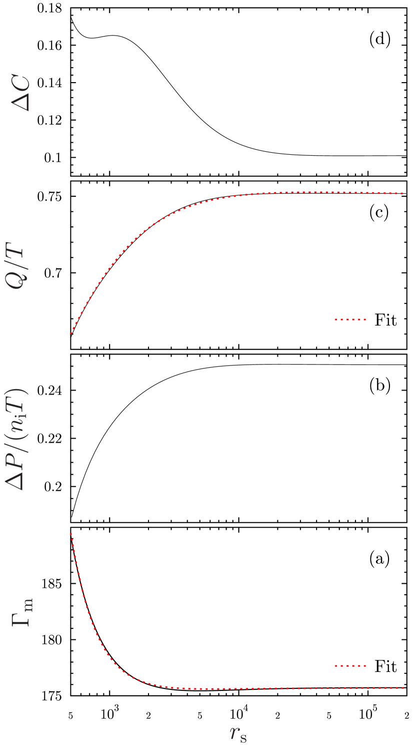
Figure 8: Coulomb coupling strength at melting $\Gamma_{\rm m}$ (panel a), pressure jump at melting, specified as $F_{\rm liq}=F_{\rm sol}$, in units of $n_{\mathrm{i}}T$ (panel b), latent heat $Q$ in units of $T$ (panel c), and specific heat jump at melting $\Delta C$ (panel d) vs. $r_{\mathrm{s}}$.

The Coulomb coupling parameter at melting, $\Gamma_{\rm m}$, obtained in this way as a function of $r_{\mathrm{s}}$, is shown in panel (a) of Fig. 8. The dependence of $\Gamma_{\rm m}$ on $r_{\mathrm{s}}$ can be approximated by the following analytic expression

$$\Gamma_{\rm m}=175.7-\frac{1300}{r_{\mathrm{s}}}+\frac{4.1\times 10^{6}}{r_{\mathrm{s}}^{2}}~{}.$$ (40)

This formula is plotted by dots in panel (a) of Fig. 8. It fits our numerical results in the range $500\leq r_{\mathrm{s}}\leq 120000$.

In Fig. 9, we show the temperature-density plane as $100/r_{\mathrm{s}}$ versus $T/{\rm Ry}$ (${\rm Ry}=0.5m_{\mathrm{i}}Z_{\mathrm{i}}^{4}e^{4}/\hbar^{2}=0.5T\Gamma r_{\mathrm{s}}$ is the ion Rydberg). In this plot, long-dashed line is the crystallization curve predicted by Chabrier (1993), short-dashed line is the prediction of Jones & Ceperley (1996), and solid line is the present prediction. Evidently, our prediction is closer to the result of Chabrier (1993), but is not exactly the same.

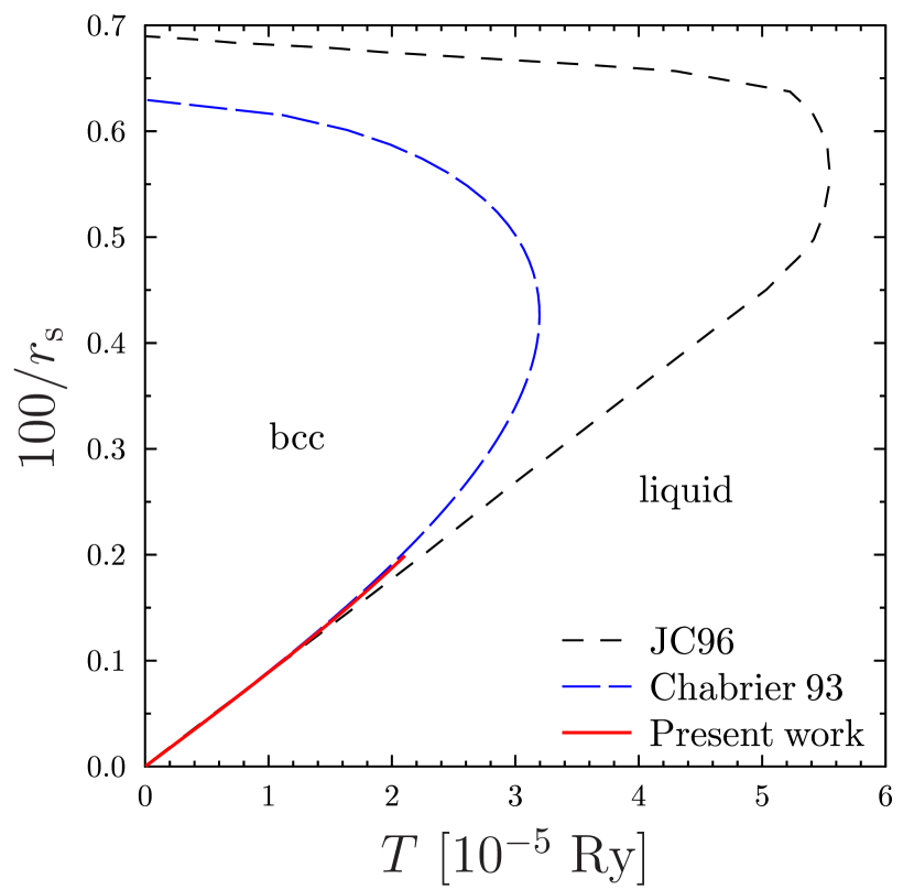
Figure 9: Phase diagram of the OCP. Long and short dashes are melting temperature predictions by Chabrier (1993) and Jones & Ceperley (1996), respectively. Solid line describes present results.

In reality though, a coexistence of phases is only possible at pressures equal on both sides, and the melting transition must be studied at a constant total pressure in both phases rather than at a fixed ion (and electron) density. The assumption of a fixed density implies an ion pressure jump between the phases, $\Delta P=P_{\rm liq}-P_{\rm sol}$. This jump can be easily calculated by combining the harmonic pressure from Paper I with present equations (29) and (36). It is shown in panel (b) of Fig. 8. In order to compensate the ion pressure jump, the density of the solid phase must be slightly higher, so that the electron pressure in the solid phase becomes higher than in the liquid. The required density increase is given by

$$\delta n_{\mathrm{i}}=\Delta P\frac{\partial n_{\mathrm{i}}}{\partial P_{\rm sol}}~{},$$ (41)

where $P_{\rm sol}$ is the total solid pressure dominated by degenerate electrons. It is easy to show, that the density jump will ensure the equality of the Gibbs free energies in both phases along with the pressure equality.

Due to the density increment, the resulting $\Gamma_{\rm m}$ at melting becomes different in the liquid and solid phases, but this difference as well as the difference with the original, fixed density, $\Gamma_{\rm m}$ is extremely small. If we were to plot these quantities versus $r_{\mathrm{s}}$ in Fig. 8, the three curves would merge. Indeed, in Fig. 10, we show the fractional density jump between the liquid and solid phases as a function of $r_{\mathrm{s}}$. To calculate this quantity, we employed exact formulae for ion thermodynamic functions and the standard thermodynamics of the degenerate electron gas at $T=0$ (e.g. Haensel et al., 2007). The density jump depends on the assumed ion species, because the functional form of the density dependence of the electron pressure is sensitive to the electron relativity degree.

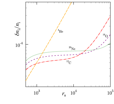
Figure 10: Fractional ion density jump upon crystallization for nuclei species typical of matter in a WD core.

If the phase transition is found from the equality of the Helmholtz free energies at fixed density (as in the beginning of this Section), one sees that the energy difference between the phases, $Q\equiv U_{\rm liq}-U_{\rm sol}>0$, is equal to $T\Delta S$. In this case, $\Delta S$ is the ion entropy difference. Introducing the density jump, equation (41), and imposing the equality of the Gibbs free energies, one sees, that the same $T\Delta S$ (ion quantities essentially do not change as a consequence of this procedure) becomes equal to the enthalpy difference between the phases also known as the latent heat of crystallization. This quantity plays an important role in astrophysics of white dwarfs. It is released as the matter in a WD core crystallizes, which delays cooling of these stars and affects various age estimates (e.g. Tremblay et al., 2019, and references therein). According to our calculations, the latent heat is a slowly varying function of $r_{\mathrm{s}}$, which is shown in panel (c) of Fig. 8. This dependence can be approximated by an analytic expression valid for $500\leq r_{\mathrm{s}}\leq 120000$, as follows:

$$\frac{Q}{T}=0.75\left(1+\frac{1.4}{\sqrt{r_{\mathrm{s}}}}-\frac{145}{r_{\mathrm{s}}}+\frac{1200}{r_{\mathrm{s}}\sqrt{r_{\mathrm{s}}}}\right)~{}.$$ (42)

This formula is plotted by dots in panel (c) of Fig. 8.

Note, that at higher $r_{\mathrm{s}}$, where ions are almost classic, our calculations indicate that $\Delta P\approx n_{\mathrm{i}}Q/3$ in agreement with theory (Hansen, Torrie & Vieillefosse, 1977). Let us also observe that $\Delta S=Q/T$ is the jump of excess entropy at melting.

Another remarkable quantity is the specific heat jump between the solid and liquid phases. In Fig. 11, we show the ion specific heat of the OCP across the phase transition. In this case, we combine updated thermodynamics of the liquid from Sec. 6, Paper I for the harmonic term in the crystal, and the results of Sec. 4 for the anharmonic contribution. Different curves correspond to different $r_{\mathrm{s}}$ values. The presence of the jump is evident and so is its $r_{\mathrm{s}}$ dependence. The dependence of the specific heat jump at melting on $r_{\mathrm{s}}$ is shown in panel (d) of Fig. 8.

Thin dot-dashed curves in Fig. 11 display the specific heat in the liquid phase obtained from the Paper III fit. It is seen to be sufficiently accurate at lower $\Gamma$ or higher $r_{\mathrm{s}}$, but gradually worsens, as one approaches the phase transition in the deep quantum regime.

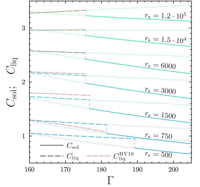
Figure 11: Specific heat of the OCP vs. $\Gamma$ for several values of $r_{\mathrm{s}}$. Discontinuity indicates melting transition. Solid curves, $C_{\rm sol}$, and dashed curves, $C_{\rm liq}$, represent the crystal and liquid phases, respectively. Dotted curves demonstrate the specific heat of a superheated crystal (at lower $\Gamma$) and a supercooled liquid (at higher $\Gamma$). Thin dot-dashed curves show the specific heat in the liquid based on the Paper III fit.

8 Astrophysical applications

As discussed in the Introduction, one-component plasma model is relevant for astrophysics of compact degenerate stars, white dwarfs and neutron stars. In these objects, matter at densities above $\sim 10-1000$ g cm^-3 (depending on the chemical composition) is fully pressure-ionized. The phase, containing bare atomic nuclei and nearly rigid, degenerate electron gas, extends all the way down to the center of a star, in the case of white dwarfs, or to the outer boundary of the inner crust (at $\rho_{\rm d}\approx 4.3\times 10^{11}$ g cm^-3), in the case of neutron stars.

The chemical elements present in such matter may vary from the lighter H, He, and C to the heavier Ne, Fe, and many other. As we saw in Secs. 3, 4, and 6, ion thermodynamics is parameterized by just two dimensionless quantities, $\Gamma$ and $r_{\rm s}$. Consequently, our fitting formulae enable one to determine all the necessary thermodynamic functions in the entire temperature and density range of astrophysical interest for any nuclear species.

Let us illustrate the results of the preceding sections by considering a few fiducial astrophysical examples. We shall focus on the total heat capacity (ion plus electron) of fully ionized matter. The ion contribution to it is probably the most practically important ion thermodynamic function, as it dominates over the electron contribution and thus has a significant impact on the thermal evolution of a star.

In Fig. 12, we plot, in physical units, the total heat capacity of dense matter composed of helium at $T=3\times 10^{5}$ K or oxygen at $T=3\times 10^{6}$ K as a function of mass density. Thick long-dashed lines describe the liquid phase. Thick solid curves is the total heat capacity of the solid phase. Dots do not include the ion anharmonic contribution, whereas thin solid curves demonstrate the total solid-phase heat capacity as parameterized by Potekhin & Chabrier (2010) but without the ion-electron contribution associated with electron screening.

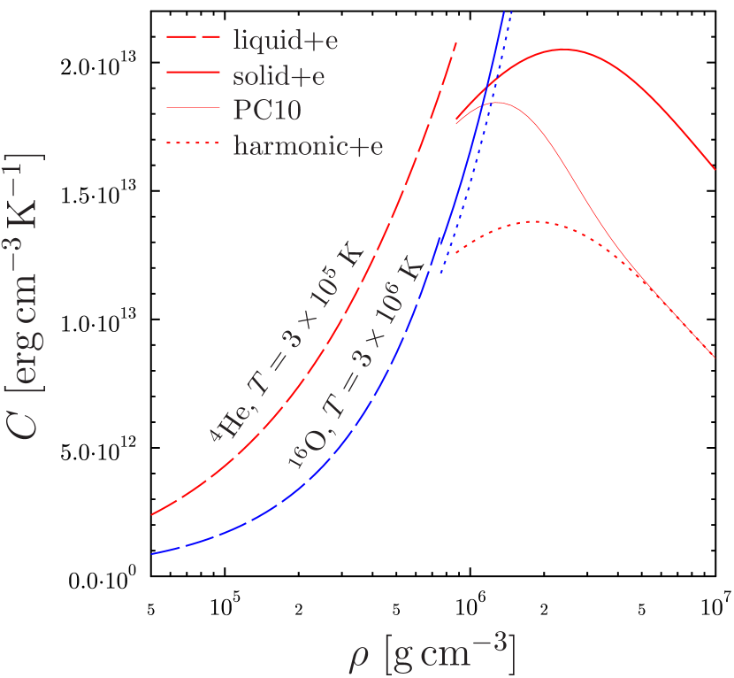
Figure 12: Total (ion plus electron) heat capacity of dense matter composed of helium at $T=3\times 10^{5}$ K or oxygen at $T=3\times 10^{6}$ K vs. mass density. Thick long-dashed and solid curves correspond to the liquid and crystal phases, respectively. Dotted lines include only ion harmonic and electron contributions. Thin solid line (merging with the thick solid line in the case of oxygen) is the parameterization of Potekhin & Chabrier (2010).

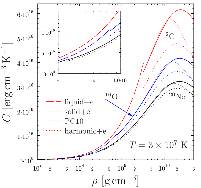
Figure 13: Same as in Fig. 12 but for carbon, oxygen, and neon plasma at $T=3\times 10^{7}$ K.

In Fig. 13, the total heat capacity of carbon, oxygen, and neon plasma at $T=3\times 10^{7}$ K is shown as a function of density. As the matter becomes hotter and the nuclei heavier, the system becomes more classic and the quantum effects are less pronounced. Nevertheless, one still observes a discrepancy with the parameterization of Potekhin & Chabrier (2010), which can over- or underestimate the actual heat capacity.

In real systems, such as matter in a WD core or an NS crust, one expects to find a mixture of several ion species rather than the OCP. In order to describe such systems from first principles, one has to introduce new free parameters (one per each additional species) and perform numerous extra simulations. Such a program for quantum plasmas requires enormous computer resources and has not been undertaken yet for exhaustive parameter space (see, however, Roggero & Reddy 2016). For the crystallized phase, there is an additional complication associated with the fact that the structure of a multi-component crystal is still not fully understood even in the classic case (see Caplan 2020 for recent progress).

9 Conclusion

We have performed detailed first-principle path-integral Monte Carlo simulations of a bcc crystal composed of ions of a single sort and rigid uniform charge-compensating electron background (one-component plasma crystal). The study was focused on the density range $500\leq r_{\mathrm{s}}\leq 120000$, covering fully-ionized layers in the interior of white dwarfs and neutron stars, at temperatures, spanning the range from the crystallization line down to $T_{\rm p}/30$. Ion quantum effects are not negligible in a large fraction of this physical parameter domain.

The crystal anharmonic energy has been extracted from the simulation results by subtracting the harmonic energy of a finite lattice. The anharmonic energy has been fitted by a convenient analytic formula (5), which incorporated available classic and quantum asymptotes.

The fitting formula has been integrated and differentiated, and explicit expressions for anharmonic contributions to the crystal Helmholtz free energy, entropy, specific heat, and pressure are given. These are equations (15), (20), (25), and (29), which should be included in evolutionary codes to ensure accurate treatment of quantum ion thermodynamics of a crystal. These formulae cover the entire crystallized region of WD or NS interior, where they supercede any previously available results.

Naturally, the effect on the results of the evolutionary codes is not expected to be drastic, because the crystal thermodynamics is dominated by the well-known harmonic and electron contributions. Nevertheless, certain thermal properties, most importantly the specific heat, will receive a boost of up to 50%, depending on density and temperature, which is potentially noticeable.

In parallel to this work, the previously available analytic description of the liquid-phase thermodynamics of the same system has been updated to include new PIMC data at $r_{\mathrm{s}}=500$ and in the vicinity of the crystallization curve. We recommend replacing equations (6) and (9) of Paper III by the present equations (31) and (36), combining equations (12)–(15) of Paper III with the present equations (34), (35), (38), and (39), and incorporating them into evolutionary codes to describe thermodynamics of a quantum ion liquid. These formulae cover the entire liquid region of WD core or NS crust, where they supercede any previously available results.

By combining the liquid and solid thermodynamics, we have analyzed in detail melting properties of the OCP with account of ion quantum effects. In particular, we have obtained from the first principles the density dependence of: (i) the Coulomb coupling strength at melting, $\Gamma_{\rm m}$; (ii) the energy jump, which is equal to the latent heat of crystallization, $Q$; (iii) the pressure jump, accompanying the phase transition, if it is determined by equating the liquid and solid Helmholtz free energies; (iv) the respective density jump, which appears in the proper formalism based on the Gibbs free energy and accompanies crystallization in real systems; and, finally, (v) the specific heat jump. All these functions are displayed in Figs. 8 and 10. The dependences of $\Gamma_{\rm m}$ and $Q$ on density have been fitted by simple analytic formulae (40) and (42).

These results are crucial for reliable modelling of thermal evolution and asteroseismology of compact degenerate stars.

Data Availability

The data underlying this article will be shared on reasonable request to the corresponding author.

Appendix A Harmonic lattice in PIMC simulations

Within the harmonic lattice approximation, the interionic interaction potential is expanded up to the second order in ion displacements from the lattice sites. Since the lattice sites correspond to equilibrium positions, the linear terms are absent, and the dynamics of the ion system can be conveniently described by a set of independent collective coordinates (phonon modes). Each mode behaves as a harmonic oscillator with the respective frequency.

In comparison with the well-known thermodynamic limit (e.g. Paper I), PIMC simulations of a crystal include a finite number of ions $N$ in a box with periodic boundary conditions. Moreover, quantum effects are modelled by the PIMC approach, i.e. by using the primitive approximation with a finite number $M$ of imaginary time slices. Thus, to subtract the harmonic energy from the PIMC data, the harmonic lattice formalism must be developed for the same finite $N$. Then, the ion motion will be still described by a set of independent collective modes, but only those phonons will be present, whose wavevectors are consistent with the periodic boundary conditions. Furthermore, each finite-$N$ phonon mode must be treated in the primitive approximation with $M$ imaginary time slices. As we demonstrate in the next two subsections, both types of finite-size effects can be accounted for analytically.

A.1 Harmonic oscillator in PIMC

Accurate thermodynamics of a harmonic oscillator (ho) with a frequency $\omega$ is well known (e.g. Dittrich & Reuter 2020; Vorontsov-Velyaminov, Nesvit & Gorbunov 1997, where the relation to the PIMC approach is explicitly analyzed). In particular, the partition function $Z_{\mathrm{ho}}=\exp(z/2)/[\exp(z)-1]$ and the energy $U_{\mathrm{ho}}=U_{\mathrm{ho}}^{0}+\hbar\omega/[\exp(z)-1]$. In this case, $z=\hbar\omega/T$ and $U_{\mathrm{ho}}^{0}=\hbar\omega/2$ is the zero-point energy.

In a PIMC simulation, quantum harmonic oscillator is modelled by a classic ring polymer with $M$ beads in an effective potential

$$H=\frac{\mu\omega^{2}}{2M}\sum_{i}r_{i}^{2}+\frac{\mu MT^{2}}{2\hbar^{2}}\sum_{i}(r_{i}-r_{i+1})^{2},$$ (43)

where $\mu$ is the mass and $r_{i}$ is a (one-dimensional) position of the $i$-th bead ($r_{M}=r_{0}$ due to the ring condition). The second term is related to the kinetic energy. Let us consider thermodynamics of this system following Vorontsov-Velyaminov & Lyubartsev (2003). The partition function of this polymer can be written in an explicit form

$$Z_{\mathrm{ho},M} = \left(\frac{M}{2\pi z}\right)^{M/2}\,\int\exp\left[-\left(\frac{M}{z}+\frac{z}{2M}\right)\sum_{i}x_{i}^{2}\right.$$ (44)

$$\left.+\frac{M}{z}\sum_{i}x_{i}x_{i+1}\right]\mathrm{d}x_{1}\ldots\mathrm{d}x_{M},$$

where coordinates $x_{i}$ are measured in natural units $\sqrt{\hbar/(\mu\omega)}$. The exponent in square brackets is a quadratic form over $x_{i}$. Changing variables to the main axes of this form, Vorontsov-Velyaminov & Lyubartsev (2003) arrive at $Z_{\mathrm{ho},M}=(\det\mathbf{A}_{M})^{-1/2}$, with the matrix

$$\mathbf{A}_{M}=\begin{pmatrix}2\,C&-1&0&\cdots&0&-1\\ -1&2\,C&-1&0&\cdots&0\\ 0&-1&2\,C&-1&\cdots&0\\ \vdots&&&\ddots&&\vdots\\ 0&\cdots&0&-1&2\,C&-1\\ -1&0&\cdots&0&-1&2\,C\\ \end{pmatrix}$$ (45)

and $C=1+(z/M)^{2}/2$. Vorontsov-Velyaminov & Lyubartsev (2003) also obtained several useful recurrent relations to determine $\det\mathbf{A}_{M}$. Using mathematical induction, we write down $\det\mathbf{A}_{M}$ in an explicit form:

$$\det\bm{A}_{M}=\sum_{i=0}^{M-1}\mathfrak{A}_{M}^{i}\left(\frac{z}{M}\right)^{2(i+1)},$$ (46)

where

$$\mathfrak{A}_{M}^{i}=2\frac{M^{2}\,(M^{2}-1^{2})\,(M^{2}-2^{2})\cdots(M^{2}-i^{2})}{(2i+2)!}.$$ (47)

Knowing the partition function, it is easy to calculate the energy of the harmonic oscillator for $M$ beads

$$U_{\mathrm{ho},M}=-\frac{\partial\ln{Z_{\mathrm{ho},M}}}{\partial(1/T)}=\frac{\hbar\omega}{2}\frac{\mathrm{d}\det\mathbf{A}_{M}}{\mathrm{d}z}\frac{1}{\det\mathbf{A}_{M}}.$$ (48)

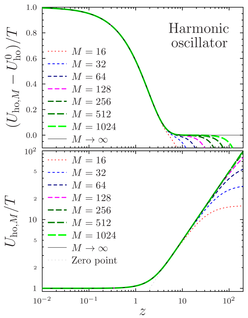
Figure 14: Energy of the harmonic oscillator $U_{\mathrm{ho},M}/T$ (bottom panel) and its “thermal energy” $(U_{\mathrm{ho},M}-U_{\mathrm{ho}}^{0})/T$ (top panel) vs. $z$ as obtained in a PIMC simulation with $M=16$, $32$, $64$, $128$, $256$, $512$, and $1024$ beads.

The energy of the harmonic oscillator, as predicted by the PIMC simulation, is shown in Fig. 14 for several values of $M$. Solid line represents the accurate quantum limit, corresponding to $M\rightarrow\infty$. Upper panel represents the “thermal energy” $(U_{\mathrm{ho}}-U_{\mathrm{ho}}^{0})/T$. One can see, that the PIMC simulation, for a fixed $M$, can reproduce the accurate quantum energy only up to some value $z$. At higher $z$, it strongly underestimates the energy (in particular, it does not reproduce the zero-point energy). It is worth noting, that for $zM\lesssim 1$, the difference between the PIMC energy and the exact quantum energy is well fitted (with an error of less than $0.01\hbar\omega$) by

$$U_{\mathrm{ho},M}-U_{\mathrm{ho}}=-\frac{\hbar\omega}{16}\frac{z^{2}}{M^{2}}.$$ (49)

A.2 Finite-size effects for harmonic lattice

We consider a bcc lattice and a cubic simulation box, thus, the number of ions in simulation $N=2N_{L}^{3}$, where $N_{L}$ is the number of cubic cells in each direction of the simulation box. Obviously, the box size is $L=N_{L}a_{1}$, where $a_{1}$ is the size of the bcc cubic cell. Thanks to the symmetry of the bcc lattice, it suffices to consider phonons only from the so-called irreducible part of the Brillouin zone, which is $1/48$-th of the whole Brillouin zone (e.g. Albers & Gubernatis 1981). Their wavevectors can be specified as: $\bm{k}=(2\pi i_{x}/L,2\pi i_{y}/L,2\pi i_{z}/L)$, where $i_{x}=0,\ldots,N_{l}$, $i_{y}=0,\ldots,\min(i_{x},N_{L}-i_{x})$, $i_{z}=0,\ldots,i_{y}$.

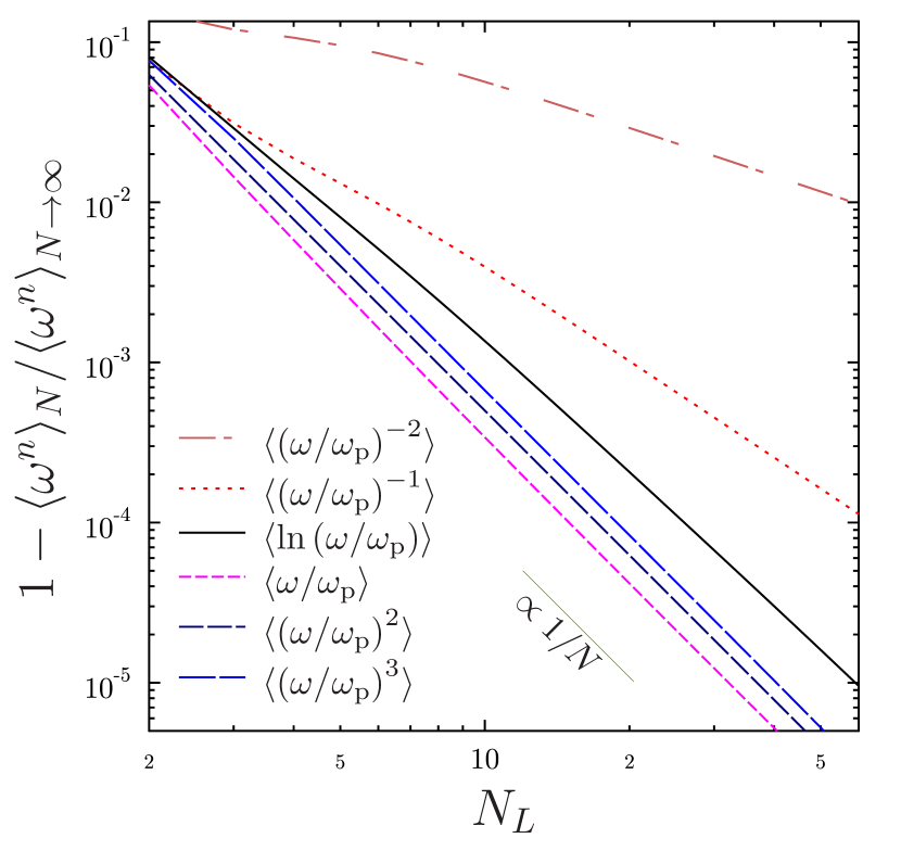
Figure 15: The relative finite-size correction for several phonon frequency moments as a function of $N_{L}$. Thin solid line indicates a $\propto 1/N=1/(2\,N_{L}^{3})$ dependence.

There are three modes for each wavevector, frequencies of these modes $\omega_{j}$ ($j=1,\ 2,\ 3$) are determined by the dynamic matrix of the bcc lattice for the OCP (see, e.g. Paper I for an explicit form). In particular, one can calculate phonon frequency moments according to

$$\langle\omega^{n}\rangle_{N}=\frac{1}{3N}\sum_{i_{x},i_{y},i_{z}}w(i_{x},i_{y},i_{z})\sum_{j}\omega_{j}^{n}~{}.$$ (50)

In this case, $w(i_{x},i_{y},i_{z})$ is the weight factor, determined by the symmetry (Wallace 1972; Albers & Gubernatis 1981). Due to finite $N$, the resulting phonon moments differ from the well known values in thermodynamic limit (see, e.g. Paper I). The relative difference is shown in Fig. 15. Note, that contribution of $k=0$ phonons was taken to be zero for all phonon moments to avoid divergence of some of them (see also below). It is the only reason there is a finite-size effect for the second moment $\langle\omega^{2}/\omega_{\rm p}^{2}\rangle_{N}$. In fact, thanks to the Kohn sum rule (Bardeen & Pines 1955; Brout 1959), $\sum_{j}\omega_{j}^{2}=\omega_{\rm p}^{2}$ for any phonon wavevector. Thus, $\langle\omega^{2}/\omega_{\rm p}^{2}\rangle_{N}\equiv 1/3-1/(3N)$, where the last term is associated with the zero contribution of $k=0$ phonons. As is obvious from Fig. 15, the relative finite-size correction for moments with a positive $n$ follows $\propto 1/N$ trend, but it is not so for $n<0$ moments and for the $\langle\ln{(\omega/\omega_{\rm p})}\rangle_{N}$ moment. This is because the dominating contribution to the latter moments comes from the vicinity of the Brillouin zone center, and thus strongly depends on the location of phonon wavevectors, available at finite $N$.

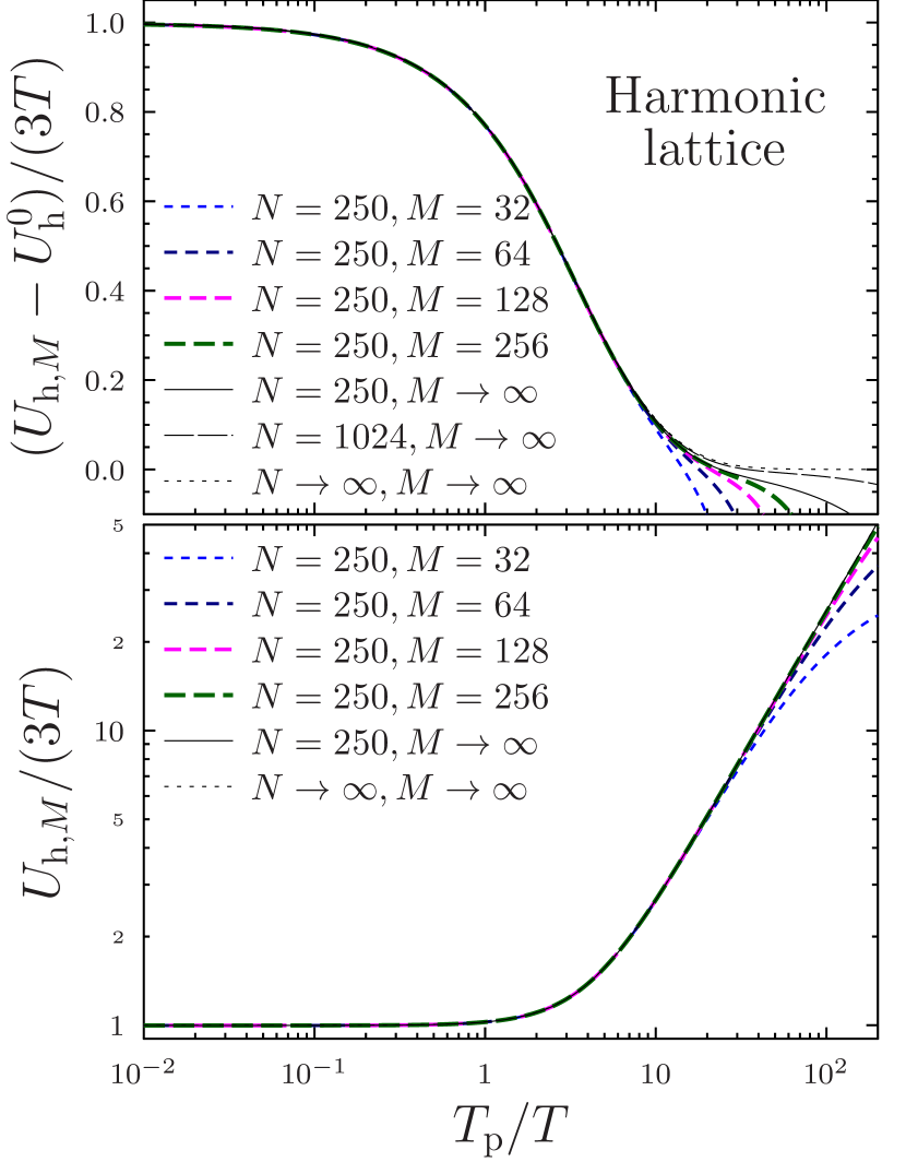
Figure 16: Harmonic lattice energy $U_{\mathrm{h},M}/(3T)$ (bottom panel) and “thermal energy” $(U_{\mathrm{h},M}-U_{\mathrm{h}}^{0})/(3T)$ (top panel) as functions of $T_{\mathrm{p}}/T$ for a PIMC harmonic lattice simulation with $N=250$ and $M=32$, $64$, $128$, or $256$ beads. Thin dotted line corresponds to the accurate quantum thermodynamic limit, while thin solid and long-dashed lines provide an accurate quantum description ($M\rightarrow\infty$) of finite systems with 250 and 1024 particles, respectively.

The harmonic energy per one ion is calculated as

$$U_{\mathrm{h},M}=\frac{1}{N}\sum_{i_{x},i_{y},i_{z}}w(i_{x},i_{y},i_{z})\sum_{j}U_{\mathrm{ho},M}(\omega_{j},T).$$ (51)

$U_{\mathrm{ho},M}(\omega_{j},T)$ is the energy given by equation (48). Note, however, that modes with ${\bm{k}}=0$ require special attention. They correspond to a motion of all ions together, i.e. a motion of the center of mass. As long as we consider only interionic interactions, it is a free motion not constrained by any forces. Obviously, the contribution of ${\bm{k}}=0$ modes must be equal to $3T/2$.

The resulting harmonic lattice energy as a function of $T_{\mathrm{p}}/T$ (cf. Sec. 3) is shown in the bottom panel of Fig. 16. The dotted line represents the energy in the thermodynamic limit (Paper I); in the scale of the bottom panel, it coincides with the solid line, which represents accurate quantum description for $N=250$. Similar to the harmonic oscillator (Fig. 14), PIMC underestimates the energy at low $T$ due to a finite number of beads.

To demonstrate the importance of the finite-size effects in the strongly quantum regime ($T\ll T_{\mathrm{p}}$), in the top panel of Fig. 16, we plot $(U_{\mathrm{h},M}-U_{\mathrm{h}}^{0})/3T$ as a function of $T_{\mathrm{p}}/T$. In this case, $U_{\mathrm{h}}^{0}/N=\hbar\omega_{\mathrm{p}}\langle\omega/\omega_{\mathrm{p}}\rangle/2$ is the zero-point energy calculated in the thermodynamic limit (the first frequency moment $\langle\omega/\omega_{\mathrm{p}}\rangle=0.5113875$, Paper I). As it should be, in the thermodynamic limit, this difference represents the thermal energy and it is positive (see the dotted line). However, it is not the case for the finite-$N$ simulation, even if the quantum effects are included accurately ($M\rightarrow\infty$, see thin solid line). This is because the first frequency moment for $N=250$ ($N_{L}=5$) is a bit lower: $\langle\omega/\omega_{\mathrm{p}}\rangle_{250}=0.5099073$ (as expected, the correction is of the order of $1/N$, see Fig. 15). Usage of a finite number of beads $M$ in a PIMC simulation makes agreement with the thermodynamic limit even worse. That is why we use $U_{\mathrm{h},M}$ calculated from equation (51) to extract the anharmonic energy from our simulations. In this way, we avoid an impact of the finite-size effects in the main, harmonic, energy on the subdominant anharmonic energy.

Appendix B Extrapolation properties of the new liquid fit

In Fig. 17, we show a color map of the specific heat derived from the new fit of the liquid phase energy, equations (30) and (31), in a very broad domain of $\Gamma$ and $r_{\mathrm{s}}$, covering the solid phase as well as the extremely dense region $r_{\mathrm{s}}\ll 500$. The specific heat is explicitly positive in the extrapolated region. A minimum at $\Gamma\approx 140$ and $r_{\mathrm{s}}\approx 70$ is likely an artefact of our fit. Note however, that this artefact should not affect any astrophysical applications, because it is located far outside the region of astrophysical interest.

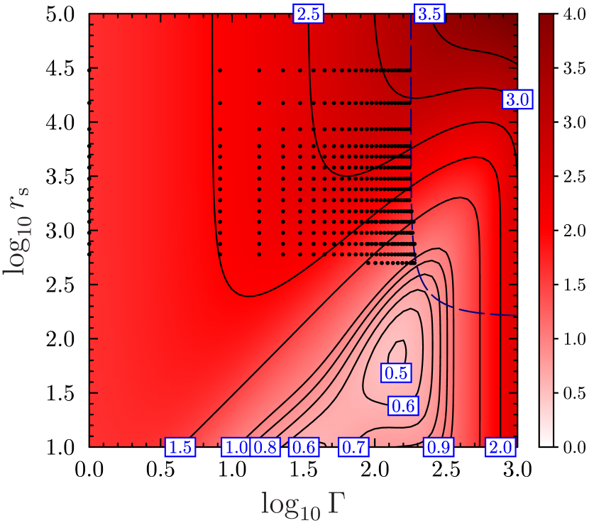
Figure 17: Color map of the ion specific heat derived from the new liquid-phase fit. Dashed line represents the melting curve, dots indicate PIMC points in the liquid, on which the fit is based.

References

- Albers & Gubernatis (1981) Albers R. C., Gubernatis J. E., 1981, Brillouin-zone integration schemes: An efficiency study for the phonon frequency moments of the harmonic, solid, one-component plasma, University of California, LA-8674-MS
- Albers & Gubernatis (1986) Albers R. C., Gubernatis J. E., 1986, Phys. Rev. B, 33, 5180 [Erratum: Albers R. C., Gubernatis J. E., 1990, Phys. Rev. B, 42, 11373]
- Baiko (2002) Baiko D. A., 2002, Phys. Rev. E, 66, 056405
- Baiko (2014) Baiko D. A., 2014, Journal of Physics: Conference Series, 496, 012010
- Baiko (2019) Baiko D. A., 2019, MNRAS, 488, 5042 (Paper II)
- Baiko (2021) Baiko D. A., 2021, MNRAS, 508, 2134
- Baiko & Yakovlev (2019) Baiko D. A., Yakovlev D. G., 2019, MNRAS, 490, 5839 (Paper III)
- Baiko et al. (2001) Baiko D. A., Potekhin A. Y., Yakovlev D. G., 2001, Phys. Rev. E, 64, 057402 (Paper I)
- Bardeen & Pines (1955) Bardeen J., Pines D., 1955, Phys. Rev., 99, 1140
- Bauer et al. (2020) Bauer E. B., Schwab J., Bildsten L., Cheng S., 2020, ApJ, 902, 93
- Blouin & Daligault (2021) Blouin S., Daligault J., 2021, arXiv e-prints, p. arXiv:2107.07094
- Blouin et al. (2021) Blouin S., Daligault J., Saumon D., 2021, ApJ, 911, L5
- Brout (1959) Brout R., 1959, Phys. Rev., 113, 43
- Caillol (1999) Caillol J. M., 1999, J. Chem. Phys., 111, 6538
- Camisassa et al. (2021) Camisassa M. E., Althaus L. G., Torres S., Córsico A. H., Rebassa-Mansergas A., Tremblay P.-E., Cheng S., Raddi R., 2021, A&A, 649, L7
- Caplan (2020) Caplan M. E., 2020, Phys. Rev. E, 101, 023201
- Caplan et al. (2020) Caplan M. E., Horowitz C. J., Cumming A., 2020, ApJ, 902, L44
- Caplan et al. (2021) Caplan M. E., Freeman I. F., Horowitz C. J., Cumming A., Bellinger E. P., 2021, ApJ, 919, L12
- Carr et al. (1961) Carr W. J., Coldwell-Horsfall R. A., Fein A. E., 1961, Physical Review, 124, 747
- Ceperley (1978) Ceperley D., 1978, Phys. Rev. B, 18, 3126
- Ceperley (1995) Ceperley D. M., 1995, Reviews of Modern Physics, 67, 279
- Chabrier (1993) Chabrier G., 1993, ApJ, 414, 695
- Chabrier et al. (1992) Chabrier G., Ashcroft N. W., Dewitt H. E., 1992, Nature, 360, 48
- Cheng et al. (2019) Cheng S., Cummings J. D., Ménard B., 2019, ApJ, 886, 100
- Chugunov & Baiko (2005) Chugunov A. I., Baiko D. A., 2005, Physica A: Statistical Mechanics and its Applications, 352, 397
- Dewitt & Slattery (1999) Dewitt H., Slattery W., 1999, Contributions to Plasma Physics, 39, 97
- Dewitt & Slattery (2003) Dewitt H., Slattery W., 2003, Contributions to Plasma Physics, 43, 279
- Dittrich & Reuter (2020) Dittrich W., Reuter M., 2020, Partition Function for the Harmonic Oscillator. Springer International Publishing, Cham, pp 317–323, doi:10.1007/978-3-030-36786-2˙26
- Dubin (1990) Dubin D. H. E., 1990, Phys. Rev. A, 42, 4972
- Dubin & O’Neil (1999) Dubin D. H., O’Neil T. M., 1999, Reviews of Modern Physics, 71, 87
- Farouki & Hamaguchi (1993) Farouki R. T., Hamaguchi S., 1993, Phys. Rev. E, 47, 4330
- Gaia Collaboration et al. (2016) Gaia Collaboration et al., 2016, A&A, 595, A1
- Gaia Collaboration et al. (2018) Gaia Collaboration et al., 2018, A&A, 616, A10
- Haensel et al. (2007) Haensel P., Potekhin A., Yakovlev D., 2007, Neutron Stars 1: Equation of State and Structure. Astrophysics and Space Science Library, Springer-Verlag, Berlin
- Hansen & Vieillefosse (1975) Hansen J. P., Vieillefosse P., 1975, Physics Letters A, 53, 187
- Hansen et al. (1977) Hansen J. P., Torrie G. M., Vieillefosse P., 1977, Phys. Rev. A, 16, 2153
- Horowitz et al. (2007) Horowitz C. J., Berry D. K., Brown E. F., 2007, Phys. Rev. E, 75, 066101
- Horowitz et al. (2010) Horowitz C. J., Schneider A. S., Berry D. K., 2010, Phys. Rev. Lett., 104, 231101
- Iyetomi et al. (1993) Iyetomi H., Ogata S., Ichimaru S., 1993, Phys. Rev. B, 47, 11703
- Jermyn et al. (2021) Jermyn A. S., Schwab J., Bauer E., Timmes F. X., Potekhin A. Y., 2021, ApJ, 913, 72
- Jones & Ceperley (1996) Jones M. D., Ceperley D. M., 1996, Phys. Rev. Lett., 76, 4572
- Khrapak & Khrapak (2016) Khrapak S. A., Khrapak A. G., 2016, Contributions to Plasma Physics, 56, 270
- Kugler (1969) Kugler A. A., 1969, Annals of Physics, 53, 133
- Lamb & van Horn (1975) Lamb D. Q., van Horn H. M., 1975, ApJ, 200, 306
- Oertel et al. (2017) Oertel M., Hempel M., Klähn T., Typel S., 2017, Reviews of Modern Physics, 89, 015007
- Ostriker & Axel (1968) Ostriker J. P., Axel L., 1968, The Astronomical Journal Supplement, 73, 31
- Potekhin & Chabrier (2000) Potekhin A. Y., Chabrier G., 2000, Phys. Rev. E, 62, 8554
- Potekhin & Chabrier (2010) Potekhin A. Y., Chabrier G., 2010, Contributions to Plasma Physics, 50, 82
- Roggero & Reddy (2016) Roggero A., Reddy S., 2016, Phys. Rev. C, 94, 015803
- Salaris et al. (2021) Salaris M., Cassisi S., Pietrinferni A., Hidalgo S., 2021, arXiv e-prints, p. arXiv:2111.09285
- Segretain et al. (1994) Segretain L., Chabrier G., Hernanz M., Garcia-Berro E., Isern J., Mochkovitch R., 1994, ApJ, 434, 641
- Stringfellow et al. (1990) Stringfellow G. S., Dewitt H. E., Slattery W. L., 1990, Phys. Rev. A, 41, 1105
- Tremblay et al. (2019) Tremblay P.-E., et al., 2019, Nature, 565, 202
- Vorontsov-Velyaminov & Lyubartsev (2003) Vorontsov-Velyaminov P. N., Lyubartsev A. P., 2003, Journal of Physics A Mathematical General, 36, 685
- Vorontsov-Velyaminov et al. (1997) Vorontsov-Velyaminov P. N., Nesvit M. O., Gorbunov R. I., 1997, Phys. Rev. E, 55, 1979
- Wallace (1972) Wallace D., 1972, Thermodynamics of Crystals. Wiley, New York, https://books.google.ru/books?id=vgXwAAAAMAAJ