Non-linear Schr$\ddot{o}$dinger equation with time-dependent balanced loss-gain and space-time modulated non-linear interaction

Abstract

We consider a class of one dimensional vector Non-linear Schr$\ddot{o}$dinger Equation(NLSE) in an external complex potential with Balanced Loss-Gain(BLG) and Linear Coupling(LC) among the components of the Schr$\ddot{o}$dinger field. The solvability of the generic system is investigated for various combinations of time modulated LC and BLG terms, space-time dependent strength of the nonlinear interaction and complex potential. We use a non-unitary transformation followed by a reformulation of the differential equation in a new coordinate system to map the NLSE to solvable equations. Several physically motivated examples of exactly solvable systems are presented for various combinations of LC and BLG, external complex potential and nonlinear interaction. Exact localized nonlinear modes with spatially constant phase may be obtained for any real potential for which the corresponding linear Schr$\ddot{o}$dinger equation is solvable. A method based on supersymmetric quantum mechanics is devised to construct exact localized nonlinear modes for a class of complex potentials. The real superpotential corresponding to any exactly solved linear Schr$\ddot{o}$dinger equation may be used to find a complex-potential for which exact localized nonlinear modes for the NLSE can be obtained. The solutions with singular phases are obtained for a few complex potentials.

I Introduction

The Non-linear Schr$\ddot{o}$dinger equation(NLSE) appears in the context of mathematical modelling of many physical phenomena in different domains of science, like optics in nonlinear media Kivshar ; Serkin ; Serkin1 , Bose-Einstein Condensates(BEC)Dalfovo ; Pitaevskii1 ; Kevrekidis ; Kengne , plasma physicsDodd , gravity wavesTrulsen , Bio-molecular dynamicsDavydov etc. NLSE exhibits solitonZabusky ; Newell ; Zakharov3 ; Infeld solutions and is an integrable system with a very rich mathematical structureSulem ; Bourgain ; Ablowitz ; Lamb . The quantized NLSE describes a hardcore Bose-gas with delta-function interaction for which various physical properties including correlations functions can be computed analyticallykorepin . Several generalisations of the NLSE have been considered to model different emerging phenomena in physics over the last few decades. For example, the NLSE with an external confining potential is known as Gross-Pitaevskii equationPitaevskii1 and is relevant in the context of BEC. The investigations on collapse and growth of quasi-condensates in NLSE with harmonic confinement offers a rich variety of mathematical structurepkg2 ; pkg3 ; Wadati . Localized, unbounded and periodic potentials have also been investigated with interesting results. The NLSE with space Abdullaev ; Sakaguchi ; Carpentier ; Beitia ; Verde ; Theocharis ; Porter and time Saito ; Kevrekidis1 ; Brazhnyi ; Berge ; Towers ; Kevrekidis2 ; Abdullaev1 ; Garcia ; Abdullaev2 ; Montesinos ; Itin ; Konotop modulated nonlinear strengths is also of immense interest in the same context.

The generalizations of NLSE based on underlying ${\cal{PT}}$-symmetryBenderl may be broadly classified into three different classes: (i) NLSE with ${\cal{PT}}$-symmetric complex confining potential, (ii) the non-local NLSE, and (iii) NLSE with LC and BLG terms. Solvable models of NLSE with ${\cal{PT}}$-symmetric complex localized potentialKonotop1 ; Shi ; Ortiz1 ; Ortiz2 ; Cruz ; Midya ; Midya1 ; Musslimani have been considered which admits soliton solutions. The investigations on ${\cal{PT}}$-symmetry breaking as a function of the system parameters reveal a host of interesting issues including the behaviour of solitons at the exceptional pointsKonotop1 . The non-local NLSEAblowitz1 is integrable and admits bright as well as dark soliton for the same range of the nonlinear strength. The non-local vector NLSE is also integrable and amenable to exact solutions and real-valued physical quantitiesds-pkg . Further, it has lead to a new branch of integrable models where non-local generalizations of previously known integrable models have been consideredpkg1 ; Ablowitz-2 ; Avadh .

The central focus of this article is on NLSE with LC and BLG terms for which, in addition to real-valued linear and nonlinear couplings, the components of NLSE are subjected to loss or gain such that the power or a modified form of it named as pseudo-power is conservedpiju . Soliton solution was found in the discrete non-linear Schr$\ddot{o}$dinger equation(DNLS) with gain and lossSuchkov . The NLSE with balanced loss and gain has been investigated over the last one decade or so and is known to admit brightBludov1 ; Driben1 and dark solitons Bludov , breathersBarashenkov ; Driben2 , rogue wavesKharif , exceptional pointsDriben2 ; Konotop1 , etc. Further, the power oscillation is observed in some specific models which may have interesting technological applicationspkg . The NLSE with time-modulated loss-gain terms have also been investigated and shown its efficiency in the stabilization of solitonsDriben2 and soliton switchingAbdullaev3 ; Abdullaev4 ; Konotop1 . The NLSE with LC and BLG has also been investigated from the viewpoint of exact solvability and exact analytical solutions of some models are constructed under specific reduction of the original equationDriben1 ; Alexeeva . Recently, a method was prescribed to construct exactly solvable models of NLSE with LC and BLG by using a non-unitary transformation which removes the LC and BLG terms completely at the cost of modifying the strength of the nonlinear termpkg . Further, the LC and BLG terms are removed completely without modifying the nonlinear term at all for some specific models for which the non-unitary transformation can be identified as a pseudo-unitary transformation. The method has been used to construct exactly solvable models exhibiting power-oscillation.

In this article, we consider a class of NLSE with time dependent LC and BLG as well as space-time modulated nonlinear term in an external complex potential. Both time dependentAbdullaev4 and constantDriben1 ; Driben2 BLG with particular types of NLSE and vanishing confining potential have been studied earlierKonotop1 . However, most of those studies are based on approximation and/or numerical methods . The sole purpose of this article is to investigate the exact solvability of a generic system for various combinations of the time-modulated LC and BLG terms, space-time modulated nonlinear strengths and external potentials.

We follow a two-step approach. The LC and the BLG terms are removed completely in the first step via a non-unitary transformation by generalizing the technique prescribed in Ref. pkg . This results in modifying the time-dependence of the nonlinear term and in general, a real-valued non-linear term becomes complex after the non-unitary transformation. We find that the LC and BLG terms are removed completely provided they have the same time-modulation. The method of separation of variables requires that the modified non-linear term is real. This is ensured by fixing the space-time modulated strengths of the nonlinear term. In the second step, the method of similarity transformation is used to investigate the solvability of the resulting equations. The method involves defining the differential equation in a new co-ordinate system accompanied by the multiplication of a scale-factor to the amplitude. This results in a system of equations with solvable limits for appropriate choice of co-ordinates and scale-factor.

We construct several exactly solvable models to exemplify the general method. The scheme for obtaining solvable limits for real and complex external potentials are different. Exact localized nonlinear modes with spatially constant phase may be obtained for a real potential for which the corresponding linear Schr$\ddot{o}$dinger equation is solvable. Exact analytical solutions with space-time dependent phase are also obtained for a few real potential. The complex potential offers more flexibility in comparison with real potential in constructing solvable models. We devise a general method based on supersymmetric quantum mechanicskhare to find a large class of complex potentials admitting localized nonlinear modes. In general, phases of the nonlinear modes are space-time dependent. Phase singularity is present in the nonlinear mode for a few systems with complex potentials.

A few model independent features of the exact solutions are the following. The exact solutions are insensitive to the detail form of the space-modulated nonlinear strength. It is not obvious whether this is specific to the ansatz chosen for obtaining exact solutions or a manifestation of some underlying symmetry. Further, the power-oscillation in time is absent for time-independent non-linear strength. There are NLSE with constant LC, BLG and nonlinear strength for which power-oscillation has been observedpkg . The class of NLSE considered in this article has nonlinear interaction which is different from the model considered in Ref. pkg . Thus, the power oscillation in time seems to be dependent on the nonlinear interaction.

The plan of the article is the following. The model is introduced in Sec. II along with Lagrangian and Hamiltonian formulations of the system. In Sec. III, the two-step approach is implemented to map the original equation into a solvable model. Explicit examples are constructed for systems without and with external real potentials in Sec. IV and V, respectively. Results pertaining to complex confining potential are presented in Sec. VI. Finally, the findings are summarized in Sec. VII with discussions and outlook. In Appendix-I, solutions of a nonlinear equation arising in the discussions of solvable models are described.

II The Model

We consider one dimensional 2-component NLSE as

$$i\psi_{1t} = -\psi_{1xx}+k^{*}(t)\psi_{2}+i\gamma(t)\psi_{1}+V(x)\psi_{1}+\left(g_{11}(x,t)|\psi_{1}|^{2}+g_{12}(x,t)|\psi_{2}|^{2}\right)\psi_{1}$$

$$i\psi_{2t} = -\psi_{2xx}+k(t)\psi_{1}-i\gamma(t)\psi_{2}+V(x)\psi_{2}+\left(g_{21}(x,t)|\psi_{1}|^{2}+g_{22}(x,t)|\psi_{2}|^{2}\right)\psi_{2}$$ (1)

where $k(t)$ is the strength of the linear coupling among the two fields and $k^{*}$ denotes the complex conjugate of $k$. The time-modulated strength of the balanced loss gain terms is $\gamma(t)$. The space-time modulated strengths of the non-linear interaction are denoted as $g_{ij}(x,t)$. In the terminology of optics, $g_{11},g_{22}$ are self phase modulation terms, while $g_{21},g_{12}$ correspond to cross-phase modulation. The external potential $V(x)$ is relevant for the mean-field description of Bose-Einstein condensates. Several ${\cal{PT}}$-symmetric complex potentials $V(x)$ exhibit many interesting phenomenon. We discuss both real and complex potentials separately in this article and choose $V(x)=s(x)+i\tilde{s}(x)$, where functions $s(x),\tilde{s}(x)$ are real. There are several solvable limits of Eq.(1), starting from the simplest case of $g_{ij}=0,k=\gamma=0$ which models the optical wave propagation under paraxial approximationGanainy ; Markis . The integrable canonical form of Manakaov-Zakharov-Schulman(MZS) systemkk ; zs is obtained for constant coefficients $g_{ij}$ with $g_{11}=g_{21},g_{12}=g_{22}$ and vanishing linear coupling, loss-gain terms and external potential. Exact solutions of MZS system with non-vanishing constant loss-gain terms and time-dependent $g_{ij}$ with specific time-modulation have been constructed via non-unitary transformationspkg . The solutions for constant $g_{ij}$ appear as a special case. The Gross-Pitaevskii equation, which provides a mean-field description of BEC, is obtained for vanishing loss-gain terms and non-vanishing $V(x)$. Several exact solutions for different choices of $V(x)$ and space-modulated nonlinear strengths have been constructedBeitia . It appears that solvable limits of Eq. (1) in its generic form, particularly with time-dependent $k,\gamma$, space-time dependent $g_{ij}$ and with or without the external potential $V(x)$, have not been investigated so far. The method of non-unitary transformationpkg will be employed to investigate solvability of Eq. (1) in its generic form.

It is convenient to rewrite Eq.(1) in a compact form in terms of the Pauli matrices $\sigma_{1},\sigma_{2},\sigma_{3}$, $2\times 2$ identity matrix $\sigma_{0}$ and two-component complex vector $\Psi(x,t)=(\psi_{1},\psi_{2})^{T}$, where the superscript ^T denotes transpose. We define projection operators $P_{\pm}=\frac{1}{2}\left(\sigma_{0}\pm\sigma_{3}\right)$ with the properties $P_{+}\Psi=(\psi_{1},0)^{T},P_{-}\Psi=(0,\psi_{2})^{T}$ and the matrices $\sigma_{\pm}:=\frac{1}{2}\left(\sigma_{1}\pm i\sigma_{2}\right)$. The matrices $P_{\pm},\sigma_{\pm}$ form a basis for $2\times 2$ matrices. We introduce a non-hermitian scalar gauge potential $A(t)$ and an operator $D_{0}$,

$$A(t)=k\sigma_{-}+k^{*}\sigma_{+}+i\gamma\sigma_{3},D_{0}:=\sigma_{0}\frac{\partial}{\partial t}+iA(t).$$ (2)

The term $i\gamma(t)\sigma_{3}\Psi$ corresponds to time-dependent BLG, while $k(t)\sigma_{-}+k^{*}(t)\sigma_{+}$ denote time-dependent LC. The time-dependence of $A(t)$ can be controlled by choosing $k(t)$ and $\gamma(t)$ appropriately. The operator $D_{0}$ resembles the temporal component of covariant derivative with non-hermitian scalar gauge-potential $A$. It may be noted that we have not included any term of the form $f(t)\sigma_{0}$ to $A$, since it can always be trivially gauged away through a $U(1)$ transformation of the form $\Psi\rightarrow e^{-i\int^{t}f(t^{\prime})dt^{\prime}}\Psi$. The $U(1)$ phase-factor $e^{-i\int^{t}f(t^{\prime})dt^{\prime}}$ does not affect the dynamical variables like power, width of the wave-packet and its speed. Thus, the form of $A$ is quite general.

Eq. (1) can be rewritten as,

$$iD_{0}\Psi = -\Psi_{xx}+V(x)\Psi+\left[\left(g_{11}(x,t)\Psi^{\dagger}P_{+}\Psi+g_{12}(x,t)\Psi^{\dagger}P_{-}\Psi\right)P_{+}\right.$$ (3)

$$+ \left.\left(g_{21}(x,t)\Psi^{\dagger}P_{+}\Psi+g_{22}(x,t)\Psi^{\dagger}P_{-}\Psi\right)P_{-}\right]\Psi$$

which is convenient for further analysis using non-unitary transformation. Defining the power $P=\Psi^{\dagger}\Psi$ and $Q=\int dxP$, it can be checked easily that $Q$ is not a constant of motion for $\gamma\neq 0$. The power-oscillation is a hallmark of some systems with balanced loss-gain and it is a manifestation of fact that $Q$ is not a constant of motion. In fact, the expression of $P$ in Ref. pkg contains a time-dependent periodic-function which becomes unity in the limit of vanishing loss-gain terms multiplied by a space-dependent function. The quantity $\tilde{Q}=\int dx\tilde{P}$ with $\tilde{P}=\Psi^{\dagger}\eta\Psi$ is a constant of motion for $\gamma\neq 0,g_{11}=g_{21},g_{12}=g_{22}$, provided the matrix $A$ is $\eta$-pseudo-hermitian, i.e. $A^{\dagger}=\eta A\eta^{-1}$. The positive-definite matrix $\eta$ for $A$ in Eq. (2) is given in Ref. pkg ; piju . The system admits a Lagrangian and Hamiltonian formulation for $g_{12}=g_{21}$:

$${\cal{L}} = \frac{i}{2}\left[\Psi^{\dagger}D_{0}\Psi-\left(D_{0}\Psi\right)^{\dagger}\Psi\right]+\frac{1}{2}\Psi^{\dagger}\left(A^{\dagger}-A\right)\Psi-{\Psi_{x}}^{\dagger}\Psi_{x}-V(x)\Psi^{\dagger}\Psi-\frac{g_{11}}{2}\left(\Psi^{\dagger}P_{+}\Psi\right)^{2}$$

$$- \frac{g_{22}}{2}\left(\Psi^{\dagger}P_{-}\Psi\right)^{2}-g_{12}\left(\Psi^{\dagger}P_{+}\Psi\right)\left(\Psi^{\dagger}P_{-}\Psi\right),$$

$${\cal{H}} = \Psi_{x}^{\dagger}\psi_{x}+V(x)\Psi^{\dagger}\Psi+\Psi^{\dagger}A\Psi+\frac{g_{11}}{2}\left(\Psi^{\dagger}P_{+}\Psi\right)^{2}+\frac{g_{22}}{2}\left(\Psi^{\dagger}P_{-}\Psi\right)^{2}+g_{12}\left(\Psi^{\dagger}P_{+}\Psi\right)\left(\Psi^{\dagger}P_{-}\Psi\right).$$ (4)

The Hamiltonian density ${\cal{H}}$ is complex-valued for $\gamma\neq 0$ and the corresponding quantum ${\cal{H}}$ is non-hermitian with appropriate quantization condition. For $g_{11}=g_{22}=g_{12}$, the Lagrangian density is invariant under global phase transformation $\Psi\rightarrow e^{i\theta\eta}\Psi,\theta\in\mathbb{R}$ and the corresponding conserved charge is $\tilde{Q}$.

III Transformation to solvable equation

The purpose of this section is to generalize the technique outlined in Ref. pkg to remove the time-modulated BLG and LC by using a non-unitary transformation. The transformation modifies the non-linear term and suitable choices of the space-time modulated coefficients lead to solvable models. We consider a transformation relating $\Psi$ to a two-component complex scalar field $\Phi$ as follows,

$$\Psi(x,t)=U(t)\Phi(x,t)$$ (5)

It will appear later that the operator $U(t)$ in general is non-unitary. The BLG and LC terms are contained only in $D_{0}\Psi$ and it can be checked that $D_{0}\Psi=U\partial_{t}\Phi$ provided $U$ satisfies the equation,

$$\frac{dU}{dt}=-iAU(t)$$ (6)

A similar equation appears in the study of scattering theory in the interaction picture and the operator analogous to $U$ in that context is known as Dyson operator, which describes the time-evolution of a state $|\Psi(t_{0})\rangle$ to $|\Psi(t)\rangle$, i.e. $|\Psi(t)\rangle=U(t,t_{0})|\Psi(t_{0})\rangle$. The operator $U$ can not be identified as Dyson operator in the present case since it maps $\Phi(x,t)$ to $\Psi(x,t)$ at the same time $t$ and the physical context is also different. However, the solution of $U$ in Eq. (6) may be obtained as an infinite series along the line of derivation of Dyson series. We are interested in a closed form expression of $U(t)$ from the viewpoint of exact solvability. This leads to the solution of $U(t)$ for specific choice of $A$ as,

$$U(t)=e^{-i\int^{t}A(t^{\prime})dt^{\prime}},\ \ \left[A,\int^{t}A(t^{\prime})dt^{\prime}\right]=0$$ (7)

Note that $U(t)$ is non-unitary, since $A(t)$ is non-hermitian. Unitary transformations have been used in physics in different contexts, particularly in the context of field theory, for past several decades. To the best of our knowledge, the use of non-unitary transformation to construct exact solution in a systematic way has not been considered earlier. Within this background, it may be noted that a unitary transformation is a change of basis in the field-space by keeping the norm fixed, while the norm is not preserved under a non-unitary transformation. This is a major difference —systems related by unitary transformation are gauge equivalent, while the same can not be claimed for systems related by non-unitary transformation. This is manifested in the result that the power of the standard Manakov system is dif- ferent from the Manakov system with balanced loss-gain, although they are connected via a non-unitary/pseudo-unitary transformationpkg . The same is true for the system considered in this article, since $\Psi^{\dagger}\Psi\neq\Phi^{\dagger}\Phi$. Similarly, one can show that the time-dependence of other observables like width of the wave-packet and its speed of growth are different for systems connected via non-unitary/pseudo-unitary trans- formation. However, for systems connected by unitary transformation, observables like power, width of the wave-packet and its growth are identical. The unitary trans- formation only mixes different components of the field leading to different expression for the solutions.

The second condition of (7) implies that $k(t)$ and $\gamma(t)$ should have the same time dependence. We choose $k(t)=\mu_{0}(t)\beta,\gamma(t)=\mu_{0}(t)\Gamma$ in terms of an arbitrary real function $\mu_{0}(t)$ and $\beta\in\mathbb{C},\Gamma\in\mathbb{R}$ leading to the following expression of $A(t)$:

$$A(t)=\mu_{0}(t)A_{0},\ A_{0}:=\beta\sigma_{-}+\beta^{*}\sigma_{+}+i\Gamma\sigma_{3}.$$ (8)

We introduce the following quantities:

$$\mu(t)=\int^{t}\mu_{0}(t^{\prime})dt^{\prime},\ \epsilon_{0}=\sqrt{{|\beta|}^{2}-\Gamma^{2}},\ \epsilon(t)=\mu(t)\epsilon_{0}.$$ (9)

The qualitative behaviour of the operator $U(t)$ primarily depends on $\epsilon_{0}$ being positive, zero and purely imaginary. We denote the corresponding $U(t)$ as $U_{+}(t),U_{0}(t)$ and $U_{I}(t)$, respectively, with the following expressions:

$$U_{+}(t) = \sigma_{0}\cos(\epsilon)-\frac{i{A}_{0}}{\epsilon_{0}}\sin(\epsilon),\epsilon_{0}>0$$

$$U_{0}(t) = \sigma_{0}-iA_{0}\mu(t)$$

$$U_{I}(t) = \sigma_{0}\cosh({|\epsilon_{0}|}\mu(t))-i\frac{A_{0}}{|\epsilon_{0}|}\sinh({|\epsilon_{0}|}\mu(t))$$ (10)

The effect of the time-dependent scale-factor $\mu_{0}(t)$ in $A$ is to change the time-modulation of $U(t)$. For a time-independent $\mu_{0}(t)$, i.e. $\epsilon(t)=\epsilon_{0}t$, the matrix $U_{+}(t)$ becomes periodic in time. However, the matrices $U_{0}(t)$ and $U_{I}(t)$ becomes unbounded and the solutions $\Psi(x,t)$ becomes unbounded even for a bounded $\Phi(x,t)$. An interesting point to note is that bounded sloutions may be obtained for all three cases, namely, $U_{+},U_{0},U_{I}$, by suitably choosing the $\mu_{0}(t)$. For example, $\mu(t)$ reduces to the Error function, i.e. $\mu(t)=erf(t)$, for the choice

$$\mu_{0}(t)=\frac{2}{\sqrt{\pi}}e^{-t^{2}}$$ (11)

and $U(t)$ corresponding to all the three cases discussed above are bounded. Thus, appropriate time-modulation may be used to stabilize a system whose unboundedness comes solely from $U(t)$.

The removal of the BLG and LC terms through the non-unitary transformation modifies the nonlinear term and imparts additional time-dependence on it. In particular, substituting the expression of $\Psi(x,t)$ in Eq. (5) into Eq. (3), yields the following

$$i\Phi_{t} = -\Phi_{xx}+V(x)\Phi+\left[K(g_{11},g_{21})\ \Phi^{\dagger}F_{+}\Phi+K(g_{12},g_{22})\ \Phi^{\dagger}F_{-}\Phi\right]\Phi,$$ (12)

where $K(\xi_{1},\xi_{2})=\xi_{1}\left(U^{-1}P_{+}U\right)+\xi_{2}\left(U^{-1}P_{-}U\right)$ and $F_{\pm}=U^{\dagger}P_{\pm}U$. With the introduction of the functions $T_{\pm}$,

$$T_{\pm}=\frac{\Gamma\mu(t)}{\epsilon^{2}}\sin^{2}(\epsilon)\pm\frac{\sin(2\epsilon)}{2\epsilon},$$ (13)

the explicit expression of $F_{\pm}$ and $K$ may be obtained as follows:

$$F_{\pm} = \left(\frac{1}{2}+\Gamma\mu(t)T_{\pm}\right)\sigma_{0}-iT_{\pm}\mu(t)\left(\beta^{*}\sigma_{+}-\beta\sigma_{-}\right)+\left(\frac{\Gamma\mu(t)}{2\epsilon}\sin(2\epsilon)\pm\frac{1}{2}\cos(2\epsilon)\right)\sigma_{3},$$

$$K(\xi_{1},\xi_{2}) = \frac{\xi_{1}+\xi_{2}}{2}\sigma_{0}+i\left(\xi_{1}-\xi_{2}\right)\mu(t)\left(\beta^{*}\sigma_{+}T_{-}+\beta\sigma_{-}T_{+}\right)+\left(\xi_{1}-\xi_{2}\right)\left(\frac{1}{2}-\frac{\mu^{2}(t){|\beta|}^{2}}{\epsilon^{2}}\sin^{2}(\epsilon)\right)\sigma_{3}$$ (14)

We have presented the above expressions for the generic allowed values of $\epsilon_{0}$ and appropriate limits may be taken depending on the physical context of the problem. It may be noted that $T_{\pm}$ is always real valued independent of whether $\epsilon_{0}$ is positive, zero or purely imaginary. Further, the operator $F_{\pm}$ is necessarily hermitian, while $K(\xi_{1},\xi_{2})$ is hermitian either for (i) $\xi_{1}=\xi_{2}$ or (ii) $\xi_{1}\neq\xi_{2},T_{+}=-T_{-}$. The condition $T_{+}=-T_{-}$ is achieved for $\Gamma\mu(t)=0$. The choice $\mu(t)=0\ \forall\ t$ is excluded, since LC as well as BLG terms also vanish in this limit. Thus, for $\xi_{1}\neq\xi_{2}$, $K(\xi_{1},\xi_{2})$ is hermitian for $\Gamma=0$. i.e. the limit of vanishing loss-gain terms. In general, the nonlinear term in Eq. (12) is non-hermitian —the non-unitary transformation involving $U(t)$ removes the loss-gain terms at the cost of introducing non-hermiticity in the non-linear term. The nonlinear term in Eq. (12) becomes hermitian either for (i) $g_{11}=g_{21},g_{22}=g_{12},\Gamma\neq 0$ or (ii)$\Gamma=0$, since both $K(g_{11},g_{21})$ and $K(g_{11},g_{21})$ are hermitian in these limits. The second condition corresponds to vanishing loss-gain term for which $U(t)$ is unitary and the result is expected. The nonlinear term for the first condition takes the form of MZS systemkk ; zs $\left[\Psi^{\dagger}\left(g_{11}P_{+}+g_{22}P_{-}\right)\Psi\right]\Psi$, which remains real-valued after the non-unitary transformation. This particular form of nonlinear interaction with $V(x)=0,\mu_{0}(t)=1$ and space-time independent $g_{11},g_{22}$ has been investigated earlierpkg .

A pertinent question at this juncture is whether or not the solution $\Psi$ of Eq. (3) corresponding to a stable solution $\Phi$ of Eq. (12) is also stable. The answer is that the transformation (5) that connects the original system described by Eq. (3) to the Eq. (12) does not alter the stability property of $\Phi$ for a bounded $U(t)$. In order to see this, we consider $\Phi(x,t)=\tilde{\Phi}(x,t)+\chi(x,t)$, where $\tilde{\Phi}(x,t)$ is an exact solution of Eq. (12) and $\chi(x,t)$ is small perturbation. Plugging the expression of $\Phi(x,t)$ in Eq. (12), we obtain the following equation in the leading order of the perturbation,

$$i\chi_{t} = -\chi_{xx}+V(x)\chi+\left[K(g_{11},g_{21})\left\{\tilde{\Phi}^{\dagger}F_{+}\chi+\chi^{\dagger}F_{+}\tilde{\Phi}\right\}+K(g_{12},g_{22})\left\{\tilde{\Phi}^{\dagger}F_{-}\chi\right.\right.$$ (15)

$$+ \left.\left.\chi^{\dagger}F_{-}\tilde{\Phi}\right\}\right]\tilde{\Phi}+\left[K(g_{11},g_{21})\tilde{\Phi}^{\dagger}F_{+}\tilde{\Phi}+K(g_{12},g_{22})\tilde{\Phi}^{\dagger}F_{-}\tilde{\Phi}\right]\chi+{\cal{O}}\left(\chi^{2}\right)$$

The Eq. (15) determines the stability of the exact solution $\tilde{\Phi}$ and the solution is stable if $\chi$ is a bound state. The exact solution of Eq, (3) corrresponding to $\tilde{\Phi}$ is $\tilde{\Psi}=U\tilde{\Phi}$. We consider $\Psi=\tilde{\Psi}+U\eta(x,t)$, where $U(t)$ is taken to be bounded in time and $\eta(x,t)$ is an arbitrary function. The perturbation to the exact solution $\tilde{\Psi}$ is $U\eta(x,t)$ and arbitrariness of the small fluctuations is contained in $\eta(x,t)$. We find after substituting the expression of $\Psi(x,t)$ in Eq. (3) and keeping only the leading order terms that $\eta$ satisfies the Eq. (15). Thus, the stability of the original Eq. (3) and the transformed Eq. (12) is governed by the same Eq. (15) and the transformation (5) can not change the stability property for a bounded $U$ in time and under identical initial conditions.

The investigations on the complete integrability of the system described by Eq. (12) is a highly nontrivial problem in presence of $V(x)$, space-time modulated nonlinear-strengths and loss-gain terms. We are interested in this article in finding solvable limits of Eq. (1) so that the exact solutions can be used in plethora of physical systems in which it appears. The reduction of Eq. (1) to Eq. (12) with a closed form expression for $U(t)$ has been performed on general ground. In order to proceed further for analyzing two-component vector non-linear Schr$\ddot{o}$dinger equation of the form given in Eq. (12), we use the method of separation of variables by choosing one of the standard ansatzes which is consistent with the group-theory based analysisBeitia of Eq. (12) for time-independent and real-valued nonlinear strength. We consider the solution of Eq. (12) as,

$$\Phi(x,t)=W\ R(x)\ e^{i\big{(}\theta(x)-Et\big{)}},$$ (16)

where $W=(W_{1}e^{i\theta_{1}},W_{2}e^{i\theta_{2}})^{T}$ is a two-component constant, complex vector, $R(x)$ and $\theta(x)$ are real functions of their arguments and $E$ is a constant. Inserting the above expression into Eq. (12) we find,

$$R_{xx} = -i\left(R\theta_{xx}+2R_{x}\theta_{x}-R\tilde{s}(x)\right)-\left(E-s(x)\right)R+R\theta^{2}_{x}$$ (17)

$$+ \frac{1}{W^{\dagger}W}\left[W^{\dagger}K(g_{11},g_{21})W\ W^{\dagger}F_{+}W+W^{\dagger}K(g_{12},g_{22})W\ W^{\dagger}F_{-}W\right]R^{3}(x).$$

It is to be noted that in general the potential $V(x)$ in Eq.(12) is complex and has the form $V(x)=s(x)+\tilde{s}(x)$. The nonlinear term is complex and time-dependent. The method of separation of variables with the ansatz as above fails unless the coefficient of the nonlinear term is real and time-independent, which can be achieved with the judicious choice of the space-time modulated coefficients $g_{ij}(x,t)$. The imaginary part of the coefficient vanishes for the condition,

$$\frac{g_{11}-g_{21}}{g_{12}-g_{22}}=-\frac{W^{\dagger}F_{-}W}{W^{\dagger}F_{+}W}$$ (18)

while the real part of the coefficient of the nonlinear term is time-independent and equals to $f(x)=\frac{1}{2}\left(f_{1}(x)+f_{2}(x)\right)$ provided,

$$g_{11}+g_{21}=\frac{f_{1}(x)}{W^{\dagger}F_{+}W},\ \ g_{12}+g_{22}=\frac{f_{2}(x)}{W^{\dagger}F_{-}W}$$ (19)

where $f_{1}(x)$ and $f_{2}(x)$ are arbitrary functions. The space-time modulated strength $g_{ij}$ of the nonlinear interaction may be obtained by solving Eqs. (18) and (19) which constitute an undetermined system. We solve the equations by keeping $g_{22}(x,t)$ arbitrary:

$$g_{11}(x,t) = \frac{1}{W^{\dagger}F_{+}W}\left[f_{1}(x)-f(x)+g_{22}(x,t)W^{\dagger}F_{-}W\right],$$

$$g_{21}(x.t) = \frac{1}{W^{\dagger}F_{+}W}\left[f(x)-g_{22}(x,t)W^{\dagger}F_{-}W\right],$$

$$g_{12}(x.t) = \frac{1}{W^{\dagger}F_{-}W}\left[f_{2}(x)-g_{22}(x,t)W^{\dagger}F_{-}W\right]$$ (20)

It should be emphasized that each choice of $g_{22}(x,t),f_{1}(x),f_{2}(x),\mu(t)$ leads to a different classes of the space-time modulation $g_{ij}$ of the nonlinear term. However, the nonlinear equation (17) depends only on $f(x)$ and does not keep track of the specific forms of $g_{22}(x,t),f_{1}(x),f_{2}(x)$, and hence of $g_{ij}$, for fixed $f(x)$. This implies that the spatial dependence of the solution of Eqn. (1) in terms of $R(x)$ and $\theta(x)$ is same for a large class of models characterized by different $g_{ij}$. This result is very important, since solvability of Eq. (17) leads to solvability of a very large class of NLSE with LC and BLG terms characterized by various forms of $g_{ij}$.

We choose a symmetric form of the $g_{ij}$ for presenting our results:

$$g_{11}=\frac{f_{1}(x)+G(x,t)}{2W^{\dagger}F_{+}W},g_{21}=\frac{f_{1}(x)-G(x,t)}{2W^{\dagger}F_{+}W},$$

$$g_{22}=\frac{f_{2}(x)+G(x,t)}{2W^{\dagger}F_{-}W},g_{12}=\frac{f_{2}(x)-G(x,t)}{2W^{\dagger}F_{-}W},$$ (21)

where $G(x,t)$ is an arbitrary function. The introduction of $G(x,t)$ is to keep track of the arbitrariness present in the solution of the undetermined system of Eqs. (18) and (19) so that the generality is not lost. The expressions for $g_{11},g_{21}$ and $g_{22}$ may be obtained by substituting $g_{22}$ from Eq. (21) in Eq. (20). The expressions for $W^{\dagger}F_{\pm}W$ are,

$$W^{\dagger}F_{\pm}W = b_{0}\left(\frac{1}{2}+T_{\pm}(t)\mu(t)D\right)+b_{3}\left[\frac{\Gamma\mu(t)}{2\epsilon}\sin(2\epsilon)\pm\frac{1}{2}\cos(2\epsilon)\right]$$ (22)

where $\beta={|\beta|}e^{i\theta_{3}}$, $b_{j}=W^{\dagger}\sigma_{j}W,j=0,1,2,3$ and the constant $D$ is defined as,

$$D\equiv\Gamma+\frac{2}{b_{0}}W_{1}W_{2}{|\beta|}\sin\left(\theta_{2}-\theta_{1}-\theta_{3}\right).$$ (23)

The time-dependence of the space-time modulated coefficients is related to the choice of $\mu(t)$ and $G(x,t)$. There are several interesting possibilities, including time-independent $W^{\dagger}F_{\pm}W=\frac{b_{0}}{2}$ for $b_{3}=D=0$. The choice $W_{1}=W_{2}\equiv W$ leads to $b_{3}=0$ and $D=0$ gives the relation $\Gamma=-{|\beta|}\sin\left(\theta_{2}-\theta_{1}-\theta_{3}\right)$. The condition $\Gamma^{2}<{|\beta|}^{2}$ for time-periodic $U(t)$ is ensured provided $\theta_{2}-\theta_{1}-\theta_{3}\neq(2n+1)\frac{\pi}{2},\ n\in\mathbb{Z}$. Thus, $g_{ij}$’s are also independent of time in this limit provided $G(x,t)$ is taken as time independent. The space-dependence may be tailored by choosing appropriate functions $f_{1}(x),f_{2}(x),G(x,t)\equiv G(x)$. The choice $G(x,t)=0$ corresponds to $g_{11}=g_{21},g_{22}=g_{12}$ which has been noted earlier as the limit for hermitian $K$.

The imaginary part of the nonlinear interaction of Eq. (17) vanishes for $g_{ij}$’s chosen as in Eq.(21). The imaginary and real parts of Eq. (17) can be separated as,

$$\Big{(}R^{2}\theta_{x}\Big{)}_{x}=\tilde{s}(x)R^{2},$$ (24)

$$R_{xx}+\big{(}E-s(x)\big{)}R-R{\theta_{x}}^{2}=f(x)R^{3}.$$ (25)

Note that the above equations are independent of $G(x,t)$, although the space-time modulated coefficients $g_{ij}$ explicitly depend on it. This is a surprising result that $G(x,t)$ has no effect at all on the solutions $\Psi$. It seems that the specific ansatz for $\Phi$ in Eq. (16) leads to this result. The system defined by Eq. (1) with $g_{ij}$ given by Eq. (21) may admit solutions which depend on the choice of $G(x,t)$. However, the chosen ansatz is not suitable for any such exploration —different analytic and/or numerical methods may have to be employed for the purpose which is beyond the scope of this article. The solutions of Eqs. (24,25) do not depend on $f_{1}(x)$ and $f_{2}(x)$ either, but on their average $f(x)$. This is again possibly related to the chosen ansatz and has to be confirmed independently through other means. The task is to solve Eqs. (24,25) for given $s(x),\tilde{s}(x)$ and $f(x)$ which characterize the forms of the potential and space-modulation of the nonlinear strengths, respectively. The method involves defining a new co-ordinate $\zeta(x)$ and expressing $R(x)$ as the product of a scale-factor $\rho(x)$ and $\zeta$-dependent function $u(\zeta)$,

$$R(x)=\rho(x)\ u\big{(}\zeta(x)\big{)},\ \zeta(x)=\int^{x}\frac{ds}{\rho^{2}(s)}.$$ (26)

The treatment for obtaining exact solutions for real and complex potentials are different and discussed separately:

Real Potential: The imaginary part vanishes, i.e. $\tilde{s}(x)=0$ and $\theta(x)$ is determined from Eq.(24) as,

$$\theta(x)=\int\frac{C}{R^{2}}dx,$$ (27)

where $C$ is an integration constant. The decoupled equation for $R(x)$ is obtained by substituting $\theta(x)$ into Eq.(25):

$$R_{xx}+\big{(}E-s(x)\big{)}R-\frac{C^{2}}{R^{3}}=f(x)R^{3}.$$ (28)

Eq. (28) reduces to the famous Ermakov-Pinney equationep for $f(x)=0$, while $C=0=s(x),f(x)=1$ leads to the standard NLSE. The equation (28) is solvable in both the limits. There is a very interesting reduction of Eq. (28) for $C=0=f(x)$ for which it reduces to the linear Schr$\ddot{o}$dinger equation. The vanishing constant $C$ implies that the phase $\theta$ is constant. The condition $f(x)=0$ can be implemented by taking $f_{2}(x)=-f_{1}(x)$, where $f_{1},f_{2}$ may be considered as constants or space-dependent. Eq. (28) reduces to the standard linear Schr$\ddot{o}$dinger equation with real potential $s(x)$ for $C=0=f(x)$. We have the important result that the system admits exact localized nonlinear modes for any $s(x)$ for which the corresponding linear Schr$\ddot{o}$dinger equation is solvable. We do not present any example in this regard. For the general case, the substitution of Eq.(26) into Eq.(28) results in the following sets of equations:

$$u_{\zeta\zeta}+mu-\frac{C^{2}}{u^{3}}-2\sigma u^{3}=0,$$ (29)

$$\rho_{xx}+\big{(}E-s(x)\big{)}\rho=\frac{m}{\rho^{3}},\ \ f(x)=\frac{2\sigma}{\rho^{6}},$$ (30)

where $m$ and $\sigma$ are real constants. The $\theta$ dependence is contained solely in Eq. (29). The solutions of Eq. (30) for a given $s(x)$ is used to fix $f(x)$ and $\xi(x)$. The equation for $u$ can be solved independently and substitutions of $\xi(x)$ along with $\rho(x)$ determines $R(x)$. Exact solutions of Eq. (29) is discussed in Appendix-I.

Note that Eq. (30) reduces to the linear Schrödinger equation with $\rho$ playing the role of the eigenfunction for $m=0$. The complete spectra of the linear equation are known for a large number of potential $s(x)$. Each eigenstate $\rho$ for a given $s(x)$ and $E$, determines $f(x)=\frac{2\sigma}{\rho^{6}}$ trivially, which corresponds to a unique Eq. (3) via the $f(x)$ dependence of $g_{ij}$. It should be noted that different $\rho$ corresponding to different $E$ for a given $s(x)$ does not correspond to linearly independent solutions of Eq. (3) for fixed $g_{ij}$, rather it defines different NLSE. Thus, the method can be used to find exact solution of a large class of NLSE given by Eq. (3). If closed from expressions for the integrations appearing in Eqs. (26) and (27) are available, a complete analytic solution for $\Psi$ may be obtained. This only shows that Eq. (3) with a wide class of nonlinear strengths are amenable to exact solutions by using the method proposed herein. We shall present only a physically relevant prototype for a given $V(x)$ and $f(x)(g_{ij})$ to exemplify the general method in Sec. V & VI.

Complex Potential: The function $\theta(x)$ can not be expressed as the integral of $R(x)$ alone due to non-vanishing imaginary part of the potential i.e. $\tilde{s}(x)\neq 0$. Substitution of Eq.(26) into Eq.(25) results in the following sets of equations

$$u_{\zeta\zeta}+mu-2\sigma u^{3}=0$$ (31)

$$\frac{\rho_{xx}}{\rho}+E-{\theta_{x}}^{2}-\frac{m}{\rho^{4}}=s(x),\ \ f(x)=\frac{2\sigma}{\rho^{6}},$$ (32)

which are completely different from Eqs. (29,30) for the case of real potential. The effect of the imaginary part is contained in Eq. (32) via $\theta_{x}$ and taking the limit of vanishing $\tilde{s}(x)$ does neither reproduce Eq. (30) nor a decoupled equation for $\rho$ is obtained. The scheme for constructing the solvable system is the following —we fix $g_{ij}$ by choosing constant $f(x)$, say $f(x)=2\sigma$ for simplicity, which determines $\rho$, and a relation between $\theta_{x}$ and $s(x)$,

$$\theta_{x}^{2}=E-m-s(x).$$ (33)

The complex potential is chosen such that the Eqs.(24, 25) and (33) are consistent. This prescription is applicable for specific choices of $g_{ij}$ and complex potentials, nevertheless, it exhausts a large class of exactly solvable models.

The solution of Eq. (1) has the form,

$$\Psi(x,t)=U(t)\ W\ \rho(x)\ u\big{(}\zeta(x)\big{)}\ e^{i(\theta(x)-Et)},$$ (34)

where the expressions for $\rho(x),u(\zeta)$ is determined from Eqs. (29,30) for the real potential and from Eqs. (31,32) for the complex potential. The power $P(x,t)$ is factorised in terms of time-dependent and space-dependent parts as,

$$P(x,t)=P_{1}(t)R^{2}(x),P_{1}(t)\equiv W^{\dagger}U^{\dagger}(t)U(t)W.$$ (35)

The time-dependent part $P_{1}(t)$ is solely determined in terms of the non-unitary matrix $U$ and has the expression:

$$P_{1}(t)=b_{0}\left[1+\frac{2\Gamma D}{\epsilon_{0}^{2}}\sin^{2}(\epsilon)+\left(\frac{b_{3}\Gamma}{b_{0}\epsilon_{0}}\right)\sin(2\epsilon)\right]$$ (36)

The expression of $P_{1}(t)$ for constant $k$ and $\gamma$ for which $\mu(t)=t,\epsilon=\epsilon_{0}t$ has been obtained earlierpkg . The effect of allowing $k$ and $\gamma$ to have identical time dependence specified by the common scale factor $\mu_{0}(t)$ is solely contained in the argument of the sine function. The power-oscillation vanishes for $b_{3}=0,D=0$ which is also the limit for time-independent $W^{\dagger}F_{\pm}W=\frac{b_{0}}{2}$.

IV Systems without external potential $V(x)$

We have described the general method for obtaining analytic solutions of Eq. (1) in section III. In this section, we present some specific examples for $V(x)=0$ by considering time-independent and time-dependent LC and BLG terms separately. The case of non-vanishing $V(x)$ will be considered in the next section.

IV.1 Time-independent LC and BLG terms

We consider time-independent LC and BLG terms for which $\mu_{0}$, $k=\mu_{0}\beta$ and $\gamma=\mu_{0}\Gamma$ are constants. The expression of the non-unitary matrix $U(t)$ may be obtained by adjusting Eqs. (9) and Eq.(10) as,

$$U(t)=\sigma_{0}\cos(\epsilon_{0}t)-\frac{iA_{0}}{\epsilon_{0}}\sin(\epsilon_{0}t)$$ (37)

where we have chosen $\mu_{0}=1$ without loss of any generality. The time-dependent function $\epsilon(t)$ appearing in the expression of $P_{1}$ in Eq. (36) takes the form $\epsilon(t)=\epsilon_{0}t$. The space-time modulations of the nonlinear strength are discussed by considering (i) constant, (ii) purely time-dependent, (ii) purely space dependent and (iv) space-dependent $g_{ij}$ separately.

IV.1.1 Constant $g_{ij}$

The functions $g_{ij}$ in Eq. (21) are space-time independent provided $f_{1},f_{2},G$ and $W^{\dagger}F_{\pm}W$ are chosen to be constants. It may be recalled that $W^{\dagger}F_{\pm}W=\frac{b_{0}}{2}$ is constant for $W_{1}=W_{2}$ and $D=0$, i.e. $\Gamma=-{|\beta|}\sin\left(\theta_{2}-\theta_{1}-\theta_{3}\right)$. The expressions of $g_{ij}$ for these choices are obtained as,

$$g_{11} = \frac{1}{b_{0}}(f_{1}+G)\ ;\ g_{21}=\frac{1}{b_{0}}(f_{1}-G)$$

$$g_{22} = \frac{1}{b_{0}}(f_{2}+G)\ ;\ g_{12}=\frac{1}{b_{0}}(f_{2}-G)$$ (38)

where the constants $f_{1},f_{2},G$ may be chosen independently for describing different physical situations. For example, the choice $f_{1}=f_{2}$ leads to $g_{11}=g_{22}\equiv g,g_{12}=g_{21}\equiv\tilde{g}$. The system admits a Lagrangian-Hamiltonian formulation for $g_{12}=g_{21}$ and the relevant expressions are given in Eq. (4). In the terminology of optics, $g$ and $\tilde{g}$ may be identified as self-phase modulation and cross-phase modulation, respectively. The self-phase and cross-phase modulation terms may be made vanishing by choosing $f_{1}=f_{2}=G$ and $f_{1}=f_{2}=-G$, respectively. The nonlinear interaction becomes $SU(2)$ invariant for the choice $f_{1}=f_{2},G=0$ for which $g=\tilde{g}$. This particular system has been studied earlier in the context of optics and to the best of our knowledge, no exact solution has been found for generic values of $g_{ij}$. We present below exact analytical solutions for arbitrary $g_{ij}$ for the first time, which automatically includes the specific values of $g_{ij}$ discussed above.

With the choice of $f=\frac{1}{2}(f_{1}+f_{2})\equiv 2\sigma$ and $V(x)=0$, Eq.(28) reduces to,

$$R_{xx}+ER-\frac{C^{2}}{R^{3}}-2\sigma R^{3}=0,$$ (39)

which is exactly solvable. Hence, no further transformation as in Eq.(26) is required. The exact solutions of Eq. (39) is discussed in Appendix-I. We denote the solutions of Eq. (39) for $C=0,E<0,\sigma<0$ as $R_{0}(x)$ with its analytical expression given by,

$$R_{0}(x)=\sqrt{\frac{|E|}{|\sigma|}}\operatorname{sech}\left(\sqrt{|E|}x\right)$$ (40)

The solution describes a soliton and has been obtained earlierDriben2 . We present new solutions by taking $C\neq 0$ and $\sigma\geq 0$. For $\sigma=0$, i.e. $f_{1}=-f_{2}$, Eq. (39) is the famous Ermakov-Pinney equation and admits periodic solution $R_{P}(x)$ for $E>0$,

$$R_{P}(x) = \sqrt{\sin^{2}(\sqrt{E}x)+\frac{C^{2}}{E}\cos^{2}(\sqrt{E}x)},\ E>0.$$ (41)

while diverges for $E<0$. The solutions of Eq. (39) for $\sigma>0$ are expressed in terms of Weierstrass Elliptic functions and choosing $\sigma=1$ for simplicity, one of the solutions reads,

$$R(x)=\sqrt{Q_{1}+(Q_{2}-Q_{1})sn^{2}(\lambda x,r)},$$ (42)

where $\lambda=\sqrt{Q_{3}-Q_{1}}$, $r^{2}=\frac{Q_{2}-Q_{1}}{Q_{3}-Q_{1}}$ and $Q_{1},Q_{2},Q_{3}$ are constants depending on the arbitrary real constants $E$, $C$, $\sigma$. Thus, the constants $Q_{i}$’s may be chosen conveniently by fixing the values of $E,C,\sigma$. The solution is chosen to be bounded as $0<Q_{1}\leq R^{2}\leq Q_{2}<Q_{3}$. In the limit $Q_{3}\rightarrow Q_{2}$, the solution reduces to

$$R(x)=\sqrt{Q_{1}+(Q_{2}-Q_{1})\tanh^{2}(\lambda x)}.$$ (43)

Following the discussions in Appendix-I, other solutions may be written down easily. The power $P$ of the system for constant $g_{ij}$ is time independent, i.e. $P=b_{0}R^{2}$, where $R$ is given by Eq. (42) or in the limit $Q_{3}\rightarrow Q_{2}$ by Eq. (43). The power-oscillation in time has been observed for models described in Ref. pkg where the nonlinear potential is of the form $(\Psi^{\dagger}M\Psi)^{2}$ where the scalar gauge potential $A$ is pseudo-hermitian with respect to the constant matrix $M$, i.e. $A^{\dagger}=MAM^{-1}$. The nonlinear potential defined by $g_{ij}$’s in Eq. (38) can not be cast in the form $(\Psi^{\dagger}M\Psi)^{2}$ for some $M$ and the absence of power oscillation for the present case is not in contradiction with the results of Ref. pkg .

IV.1.2 Purely time-dependent $g_{ij}$

We consider Eq.(1) with purely time-dependent nonlinear strengths by choosing $g_{ij}$’s to be dependent on time alone. It may be recalled that time dependent non-linear strength arises in optics for transverse beam propagation in layered optical mediaBerge ; Towers . Further, NLSE with periodic time variation of nonlinear strength in an external magnetic field has been used to produce matter wave breathers in quasi one-dimensional Bose-Einstein condensateKevrekidis2 . As evident from Eq. (21), purely time dependent $g_{ij}$’s may be obtained by taking $f_{1},f_{2}$ as constants and allowing $G$ to be a function of time only. For simplicity, we consider $\theta_{2}-\theta_{1}-\theta_{3}=n\pi$ and $W_{1}=W_{2}$, for which the expressions of $g_{ij}$ are,

$$g_{11} = \frac{f_{1}+G(t)}{b_{0}(1+2\Gamma q_{+})},\ \ g_{21}=\frac{f_{1}-G(t)}{b_{0}(1+2\Gamma q_{+})},$$

$$g_{22} = \frac{f_{2}+G(t)}{b_{0}(1+2\Gamma q_{-})},\ \ g_{12}=\frac{f_{2}-G(t)}{b_{0}(1+2\Gamma q_{-})},$$ (44)

where $q_{\pm}$ are given as,

$$q_{\pm}=\frac{\Gamma}{\epsilon^{2}_{0}}\sin^{2}(\epsilon_{0}t)\pm\frac{\sin(2\epsilon_{0}t)}{2\epsilon_{0}}.$$ (45)

The functions $q_{\pm}$ introduce periodic time-modulation of the nonlinear strengths. Eq.(28) reduces to Eq.(39) for this case also, since $f_{1},f_{2}$ are constants and $V(x)=0$. Consequently, $R(x)$ have the expressions given by Eqs. (40), (42) and (43) for the specified choices of the constants. Unlike the case of constant $g_{ij}$, the power is time-dependent,

$$P=b_{0}\left[1+\frac{2\Gamma^{2}}{\epsilon_{0}^{2}}\sin^{2}(\epsilon_{0}t)\right]R^{2}(x)$$ (46)

where any one of the expressions of $R$ given in Eqs. (40), (42) and (43) may be used within their ranges of validity.

IV.1.3 Purely space-dependent $g_{ij}$

It is evident from Eq. (21) that purely space-dependent $g_{ij}$’s are obtained for constant $W^{\dagger}F_{\pm}W$ and choosing purely space dependent $G(x,t)\equiv G(x)$. As discussed in Sec. III, $W^{\dagger}F_{\pm}W=\frac{b_{0}}{2}$ is constant in the limit $W_{1}=W_{2}$ and $D=0$. The space modulation is determined by the space-dependent functions $f_{1}(x),f_{2}(x)$ and $G(x)$. Unlike the previous cases, solution of Eq. (28) for arbitrary $f(x)$ necessitates the transformation given by Eq. (26) resulting in Eqs. (29,30). The solutions of Eq.(30) for $V(x)=0$ are,

$$\rho^{2}(x) = ae^{2\sqrt{|E|}x}+\frac{m}{4|E|a}e^{-2\sqrt{|E|}x},\ \ E<0$$

$$\rho^{2}(x) = a\sin^{2}(\sqrt{E}x)+\frac{m}{aE}\cos^{2}(\sqrt{E}x),\ \ E>0$$ (47)

where the constant $a>0$. The solutions for $E<0$ diverges for large $x$ and will not be considered further in this article. We consider $E>0$ and make the following choices for a simplified expression of $\rho$, $E=\frac{\omega^{2}}{4},a=(1-\alpha),m=\frac{\omega^{2}(1-\alpha^{2})}{4}$, where $\omega$ and $\alpha$ are real constants. The expressions of $\rho^{2}(x)$ and hence, $f(x)$ have the following simplified expressions,

$$\rho^{2}(x)=1+\alpha\cos(\omega x),\ \ f(x)=\frac{2\sigma}{[1+\alpha\cos(\omega x)]^{3}}.$$ (48)

The functions $f_{1}(x)$ and $f_{2}(x)$ may be chosen independently subjected to the constraint $f(x)=\frac{1}{2}(f_{1}(x)+f_{2}(x))$. We choose $f_{1}(x)=f_{2}(x)=2\sigma[1+\alpha\cos(\omega x)]^{-3}$ for which space-dependent $g_{ij}$ have the expressions,

$$g_{11}=g_{22}=\frac{G(x)}{b_{0}}+\frac{2\sigma}{b_{0}[1+\alpha\cos(\omega x)]^{3}},$$

$$g_{12}=g_{21}=-\frac{G(x)}{b_{0}}+\frac{2\sigma}{b_{0}[1+\alpha\cos(\omega x)]^{3}}$$ (49)

For $G=0$, all $g_{ij}$’s become identical. The expression of $\zeta$ is obtained by using the second equation of Eq. (26) and the first equation of (48),

$$\zeta=\frac{2}{\omega\sqrt{1-\alpha^{2}}}\ \arctan\left[\sqrt{\frac{1-\alpha}{1+\alpha}}\ \tan(\frac{\omega x}{2})\right],$$ (50)

where ${|\alpha|}<1$. It remains to find $u(\zeta)$ in order to completely specify the solution. Note that the equations (39) and (29) satisfied by $R(x)$ and $u(\zeta)$, respectively, are identical with the identification of $E\leftrightarrow m,x\leftrightarrow\zeta,R(x)\leftrightarrow u(\zeta)$. The solutions of Eq. (39) are given in Eqs. (40) and (42) which may be used to write down the solutions of $u(\zeta)$ with the identification stated above. The power $P=b_{0}\rho^{2}(x)u(\zeta)^{2}$ is independent of time.

IV.1.4 Space-time dependent $g_{ij}$

The results for space-time dependent $g_{ij}$’s have been discussed in Sec. III in detail except for the solution of Eq. (28) for $R(x)$ or equivalently of Eq. (29,30) for $u(\zeta)$ and $\rho(x)$. It may be noted that Eq. (29) is the same for purely space dependent $g_{ij}$ as well as space-time dependent $g_{ij}$. Thus, the expressions of $\{\rho(x),f(x)\}$ and $\zeta(x)$ are given by Eqs. (48) and (50), respectively, within the specified ranges of validity. The solutions for $u(\zeta)$ are given by Eqs. (40) and (42) with the replacement of $E\rightarrow m,x\rightarrow\zeta,\{R_{0}(x),R_{P}(x),R(x)\}\rightarrow\{u_{0}(\zeta),u_{P}(\zeta,u(x)\}$. The exact solution $\Psi(x,t)$ for space-time dependent $g_{ij}$ is different from purely space-dependent $g_{ij}$ due to the time-dependence. In particular, the power is time-independent for purely space-dependent $g_{ij}$, while it is time-dependent for space-time dependent $g_{ij}$ and given by Eqs. (35) and (36) with $\epsilon=\epsilon_{0}t$ and $\mu=1$.

IV.2 Time-dependent $k,\gamma$

The equations determining $R(x)$ and $\theta(x)$ are the same as in the case of constant $k,\gamma$. However, the non-unitary matrix $U(t)$, the strengths $g_{ij}$, and hence, expression of power will change depending on specific forms of $k(t)$ and $\gamma(t)$. We have already discussed solutions for $R(x)$ and $\theta(x)$ depending on constant, purely time-dependent, purely space-dependent and space-time dependent $g_{ij}$ which are valid for time-dependent $k(t),\gamma(t)$ independent of specific time-dependence. In order to avoid repetition of the same results, we present results related to $U(t),g_{ij}(t),P(t)$ for specific time-dependence of $k(t)$ and $\gamma(t)$. We choose periodic modulation of the LC and BLG terms by choosing $\mu_{0}(t)=\cos(\omega_{0}t),\omega_{0}\in\mathbb{R}$ so that,

$$\mu(t)=\frac{1}{\omega_{0}}\sin(\omega_{0}t),\ \epsilon=\frac{\epsilon_{0}}{\omega_{0}}\sin(\omega_{0}t),\ T_{\pm}(t)=\frac{\omega_{0}p_{\pm}}{\sin(\omega_{0}t)},$$

$$p_{\pm}\equiv\frac{\Gamma}{\epsilon^{2}_{0}}\sin^{2}\left(\frac{\epsilon_{0}}{\omega_{0}}\sin(\omega_{0}t)\right)\pm\frac{1}{2\epsilon_{0}}\sin\left(\frac{2\epsilon_{0}}{\omega_{0}}\sin(\omega_{0}t)\right).$$

The limit $\omega_{0}\rightarrow 0$ corresponds to constant LC and BLG terms. The expressions for $U,W^{\dagger}F_{\pm}W,g_{ij},P$ may be obtained from Eqs. (10), (22), (21) and (36), respectively by using the above expressions for $\mu(t),\epsilon(t),T_{\pm}(t)$.

The expressions of $W^{\dagger}F_{\pm}W$,

$$W^{\dagger}F_{\pm}W = \frac{b_{0}}{2}\left(1+2Dp_{\pm}\right)+\frac{b_{3}}{2}\left[\frac{\Gamma}{\epsilon_{0}}\sin\left(\frac{2\epsilon_{0}}{\omega_{0}}\sin(\omega_{0}t)\right)\pm\cos\left(\frac{2\epsilon_{0}}{\omega_{0}}\sin(\omega_{0}t)\right)\right],$$ (51)

when substituted in Eq. (21) gives the space-time dependent $g_{ij}$ for periodic time-modulation of the LC and BLG terms. Different types of space-time modulations of the nonlinear strengths $g_{ij}$ may be considered as follows:

• Constant $g_{ij}$: $D=0,b_{3}=0,(G,f_{1},f_{2})=\textrm{constant}$

• Purely time-dependent $g_{ij}$: Either $D$ or $b_{3}$ or both $D$ and $b_{3}$ are non-vanishing; $f_{1}$ and $f_{2}$ are constants and $G(x,t)\equiv G(t)$

• Purely space-dependent $g_{ij}$: $D=0=b_{3}$, $G(x,t)\equiv G(x)$

The condition $D=0$ may be imposed by using Eq. (23) which gives a specific relation among the parameters, while $b_{3}=0$ for the choice $W_{1}=W_{2}$. The functions $f_{1}(x),f_{2}(x),G(x,t)$ may be chosen as per the requirement, since they are arbitrary. The non-unitary operator $U$ and $P$ have the expressions:

$$U = \sigma_{0}\cos\left(\frac{\epsilon_{0}}{\omega_{0}}\sin(\omega_{0}t)\right)-\frac{iA_{0}}{\epsilon_{0}}\sin\left(\frac{\epsilon_{0}}{\omega_{0}}\sin(\omega_{0}t)\right)$$

$$P(x,t) = b_{0}\left[1+\frac{2\Gamma D}{\epsilon_{0}^{2}}\sin^{2}\left(\frac{\epsilon_{0}}{\omega_{0}}\sin(\omega_{0}t)\right)+\frac{b_{3}\Gamma}{b_{0}\epsilon_{0}}\sin\left(\frac{2\epsilon_{0}}{\omega_{0}}\sin(\omega_{0}t)\right)\right]R^{2}(x),$$ (52)

appropriate expressions for $R(x)$ are to be substituted for a given $g_{ij}$.

The general explicit solution of Eq. (1) for $V(x)=0$ and space-time dependent $g_{ij}$ is

$$\psi_{1}(x,t) = \left[W_{1}e^{i\theta_{1}}\cos(\epsilon)-\left\{i|\beta|W_{2}e^{i\left(\theta_{2}-\theta_{3}\right)}-\Gamma W_{1}e^{i\theta_{1}}\right\}\frac{\sin(\epsilon)}{\epsilon_{0}}\right]\sqrt{1+\alpha\cos(\omega x)}$$

$$\times \sqrt{Q_{1}+(Q_{2}-Q_{1})sn^{2}(\lambda\zeta,r)}\ e^{i\left(\theta(x)-Et\right)}$$

$$\psi_{2}(x,t) = \left[W_{2}e^{i\theta_{2}}\cos(\epsilon)-\left\{i|\beta|W_{1}e^{i\left(\theta_{1}+\theta_{3}\right)}+\Gamma W_{2}e^{i\theta_{2}}\right\}\frac{\sin(\epsilon)}{\epsilon_{0}}\right]\sqrt{1+\alpha\cos(\omega x)}$$ (53)

$$\times \sqrt{Q_{1}+(Q_{2}-Q_{1})sn^{2}(\lambda\zeta,r)}\ e^{i\left(\theta(x)-Et\right)}$$

The expression of $\zeta$ is given in Eq. (50) and $\theta(x)$ can be obtained from Eq. (27). The power $P=\Psi^{\dagger}\Psi$ is plotted in FIG. 1 for various time-modulations. The case of vanishing BLG and LC is considered Fig. 1(a) and no variation of the power with time is seen. The power-oscillation is seen in Fig. 1(b) for constatnt $\mu_{0}$ and non-vanishing $\beta,\Gamma$ satisfying ${|\beta|}>\Gamma$. The power-oscillation in time is a manifestation of the balanced loss-gain in the system. The solution $\Psi$ becomes unstable for non-vanishing $\beta,\Gamma$ satisfying $|\beta|\leq\Gamma$ and constant $\mu_{0}$. The respective plot is given in Fig 1.(c). We can manage the instability by choosing $\mu_{0}(t)$ properly. In Fig. 1(d), we have considered $|\beta|=\Gamma$ and a periodic modulation function $\mu_{0}(t)=\cos(t)$ for which $P(x,t)$ shows periodic behaviour. We have plotted power for $|\beta|=\Gamma$ and $\mu_{0}(t)=\frac{2}{\sqrt{\pi}}e^{-t^{2}}$ in Fig. 1(e) which is also bounded in time. The instability in the region $|\beta|<\Gamma$ can again be controlled by periodic modulation. In particular, the plot in Fig. 1(f) shows power oscillation for $\mu_{0}(t)=\cos t$ in the region $|\beta|<\Gamma$. The figures are shown upto time $t\approx 15$, but the stated features have been checked upto time $t\approx 200$.

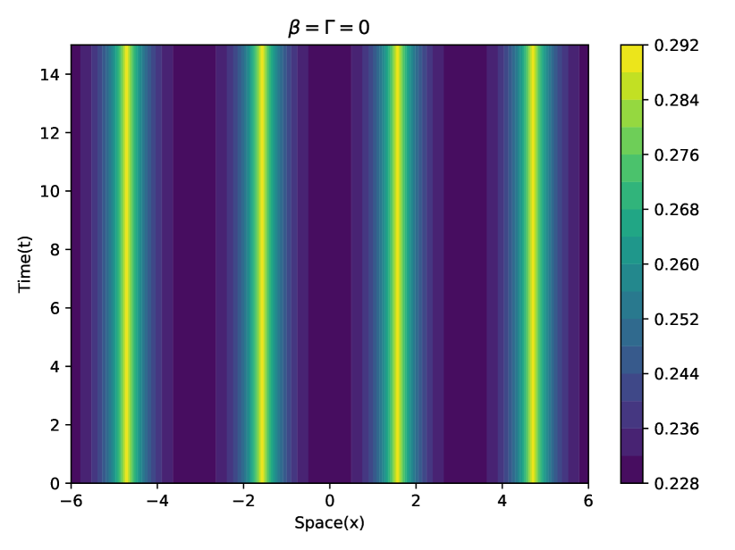
(a)

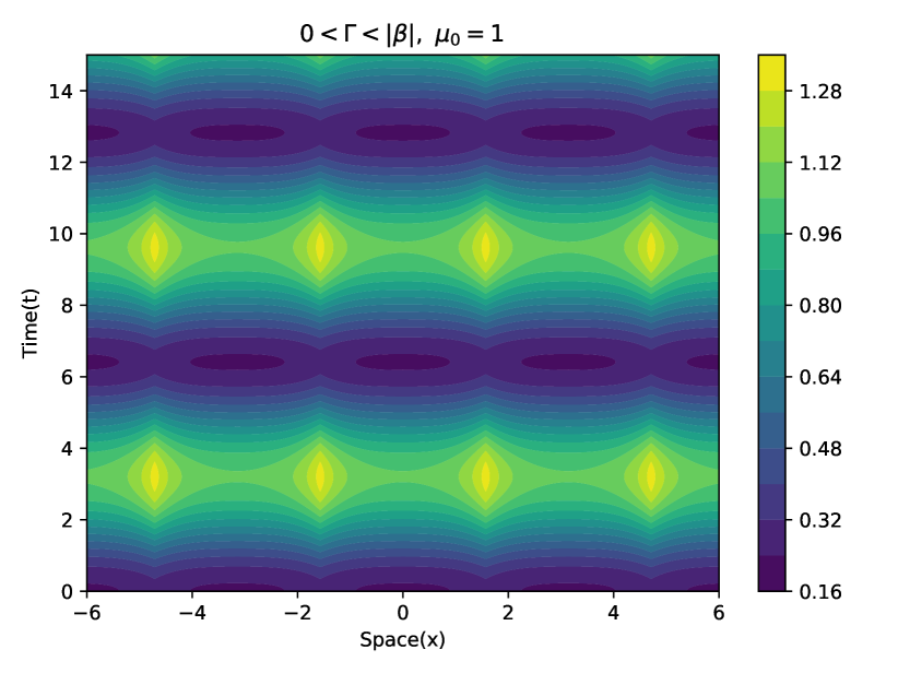
(b)

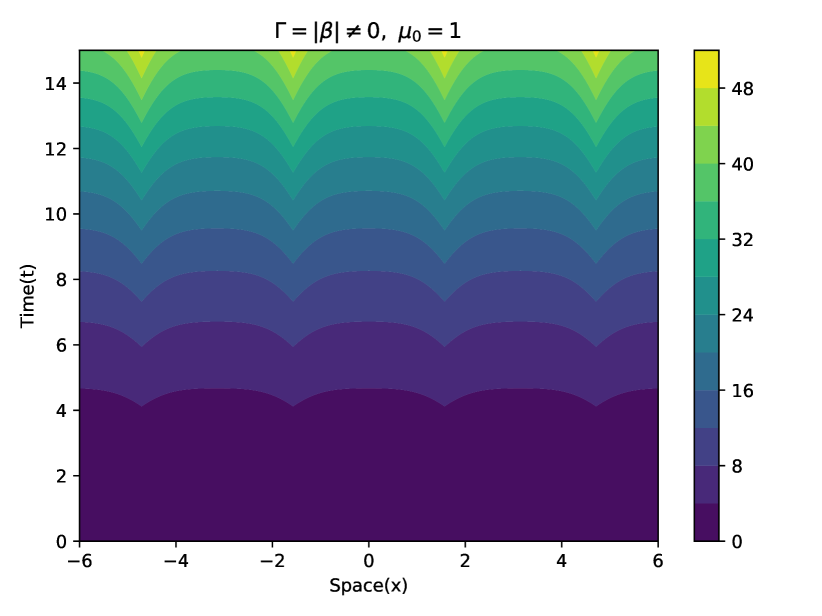
(c)

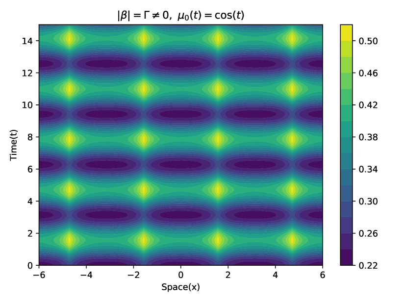
(d)

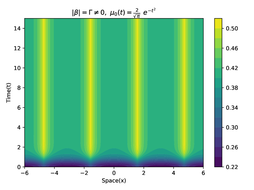
(e)

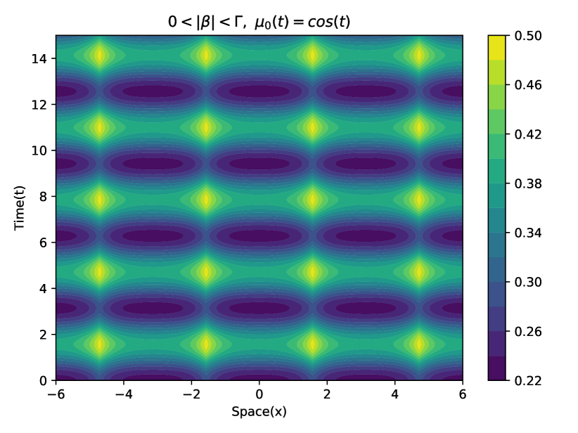
(f)

Figure 1: (Color online) Plot of Power i.e $\Psi^{\dagger}\Psi$ for $V(x)=0$ and the expression of $\Psi$ is shown in Eq. (53). Parameters: $W_{1}=W_{2}=1,\theta_{1}=\frac{\pi}{6},\theta_{2}=\frac{2\pi}{3},\theta_{3}=\frac{\pi}{3},Q_{1}=0.1,Q_{2}=0.29,Q_{3}=0.3,\sigma=1,\alpha=0.15,\omega=2$. In Fig(a): $\Gamma=|\beta|=0$, Fig(b): $\Gamma=0.5,|\beta|=0.7,\mu_{0}=1$, Fig(c): $\Gamma=|\beta|=0.5,\mu_{0}=1$, Fig(d): $\Gamma=|\beta|=0.5,\mu_{0}(t)=cos(t)$, Fig(e): $\Gamma=|\beta|=0.5,\mu_{0}(t)=\frac{2}{\sqrt{\pi}}e^{-t^{2}}$, Fig(f): $\Gamma=0.5,|\beta|=0.3,\mu_{0}(t)=cos(t)$

V Systems with Real $V(x)$

In this section, results for non-vanishing real potential $V(x)$ will be presented for purely space-dependent and space-time dependent $g_{ij}$. The method outlined in Sec. III is not suitable for constant or purely time-dependent $g_{ij}$ for which $f_{1},f_{2}$ are necessarily constants. Consequently, it follows from Eq. (30) that $f(x),\rho$ and $s(x)$ are also constants for real $V(x)$. Further, a direct solution of Eq. (28) for constant $f(x)$ and spatially varying $V(x)$ is also unknown. Within this background, we discuss a few examples of real $V(x)$ for space-time dependent $g_{ij}$ and the limit of purely space-dependent $g_{ij}$ may be considered by choosing $D=0=b_{3}$ and $G(x,t)\equiv G(x)$. The sole effect of adding a non-vanishing real potential $V(x)$ to a system with $V(x)=0$ is modified expressions of $\rho(x)$ and hence, of $\zeta(x)$ and $f(x)$. The equation determining $u(\zeta)$ remains unaffected by the choice of $V(x)$, although $u(\zeta(x))$ is dependent on the choice of $V(x)$ via $\zeta(x)$. The knowledge of $f(x)$ specifies the space-dependent part of $g_{ij}$, while space-dependent part of the power $P$ is modified due to the expression of $R(x)$ which depends on $\rho(x)$ and $u(\zeta(x))$. We present the expressions of $\rho(x),f(x),\zeta(x),u(\zeta)$ for a given $V(x)$ and do not repeat the results and discussions which have been presented in earlier sections. The space-modulated nonlinear strengths are determined in terms of $f_{1}(x)$ and $f_{2}(x)$. One may choose $f_{1}=f_{2}=f$ for simplicity or choose $f_{1}$ and $f_{2}$ such that $f(x)=\frac{1}{2}(f_{1}(x)+f_{2}(x))$ is satisfied. There is a freedom in tailoring the nonlinear strengths $g_{ij}$ for a given $f(x)$ which may be exploited to construct physically interesting systems.

V.1 Reflection-less Potential

We choose the reflection-less potential,

$$V(x)=N^{2}-N(N-1)sech^{2}(x),\ N\in\mathbb{Z}^{>}.$$ (54)

The solutions for $\rho(x)$ and $f(x)$ for $E=m=0$ may be obtained from Eq.(30) as,

$$\rho(x)=\cosh^{N}(x),\ \ f(x)=2\sigma sech^{6N}(x).$$ (55)

The potential $V(x)$ has been considered earlier in the context of single component localBeitia1 as well as non-localpkg1 NLSE. The nonlinear strengths $g_{ij}$’s may be tailored for the above $f(x)$ satisfying $\frac{1}{2}(f_{1}(x)+f_{2}(x))=f(x)$. Following the discussions in Appendix-I, the sum of the roots $Q_{1},Q_{2},Q_{3}$ is zero for $m=0$, implying that all three roots can not either be positive or negative. We choose $Q_{1}<0,Q_{2}>0,Q_{3}>0$. The solution of Eq.(29) for $\sigma=-1$ is obtained as,

$$u(\zeta)=\sqrt{Q_{3}-(Q_{3}-Q_{2})sn^{2}(\lambda\zeta,r)}$$ (56)

where $\lambda=\sqrt{Q_{3}-Q_{1}}$ and $r^{2}=\frac{Q_{3}-Q_{2}}{Q_{3}-Q_{1}}$. The expression of $\zeta$ is obtained from Eq. (26),

$$\zeta=\int\operatorname{sech}^{2N}(x)dx,$$ (57)

which can be evaluated for fixed $N$ by using the formula, $\int sech^{n}(x)=\frac{sech^{n-2}(x)tanh(x)}{n-1}+\frac{n-2}{n-1}\int sech^{n-2}(x)$ repeatedly.

V.2 Quadratic Potential

We consider the quadratic potential $V(x)=E^{2}x^{2}$ and $E>0$. For $m=0$, the solution of $\rho(x)$ and $f(x)$ is obtained from Eq.(29) as,

$$\rho(x)=e^{-\frac{1}{2}Ex^{2}},\ \ f(x)=2\ \sigma\ e^{3Ex^{2}}.$$ (58)

An unpleasant feature is that the nonlinear strengths $g_{ij}$ grow in space for this specific $f(x)$. The freedom in choosing $f_{1}(x),f_{2}(x)$ satisfying the constraint $f(x)=\frac{1}{2}(f_{1}(x)+f_{2}(x))$ and arbitrary function $G(x,t)$ is of no help to construct localized $g_{ij}$’s due to their specific dependence on $f_{1},f_{2},G$. The solutions for $u(\zeta)$ is same as (56) with the expression of $\zeta$ obtained from Eq.(26) as,

$$\zeta=\frac{1}{2}\sqrt{\frac{\pi}{E}}\ erfi(\sqrt{E}x),$$ (59)

where $erfi$ is imaginary error function. The function $\Psi(x,t)$ is finite in all regions of space, since $R(x)\rightarrow 0$ as $|x|\rightarrow\infty$. On other hand, $\Psi(x,t)$ diverges for $E<0$.

The general explicit solution of Eq. (1) for Quadratic Potential and space-time dependent $g_{ij}$ is

$$\psi_{1}(x,t) = \left[W_{1}e^{i\theta_{1}}\cos(\epsilon)-\left\{i|\beta|W_{2}e^{i\left(\theta_{2}-\theta_{3}\right)}-\Gamma W_{1}e^{i\theta_{1}}\right\}\frac{\sin(\epsilon)}{\epsilon_{0}}\right]\ e^{-\frac{1}{2}Ex^{2}}$$

$$\times \sqrt{Q_{3}-(Q_{3}-Q_{2})sn^{2}(\lambda\zeta,r)}\ e^{i\left(\theta(x)-Et\right)}$$

$$\psi_{2}(x,t) = \left[W_{2}e^{i\theta_{2}}\cos(\epsilon)-\left\{i|\beta|W_{1}e^{i\left(\theta_{1}+\theta_{3}\right)}+\Gamma W_{2}e^{i\theta_{2}}\right\}\frac{\sin(\epsilon)}{\epsilon_{0}}\right]\ e^{-\frac{1}{2}Ex^{2}}$$ (60)

$$\times \sqrt{Q_{3}-(Q_{3}-Q_{2})sn^{2}(\lambda\zeta,r)}\ e^{i\left(\theta(x)-Et\right)}$$

The expression of $\theta(x)$ is obtained from Eq. (27). The qualitative behaviour of the plots for identical $\mu_{0}(t)$ and condition on $\beta,\Gamma$ are the same with that of Fig. 1. There is no power oscillation for vanishing $\beta,\Gamma$ as seen in Fig. 2(a). The power-oscillation is seen in Fig. 2(b) for constant $\mu_{0}$ and ${|\beta|}>\Gamma$. The solution grows without any upper bound for constant $\mu_{0}$ and ${|\beta|}=\Gamma$ as is evident from Fig. 2.(c). The management of instabilities for ${|\beta|}\leq\Gamma$ by choosing suitable $\mu_{0}(t)$ is shown in Figs. 2(d), 2(e) and 2(f).

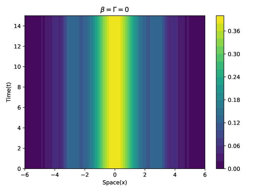
(a)

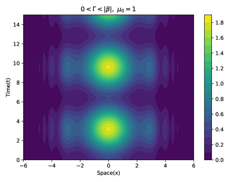
(b)

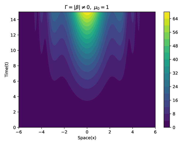
(c)

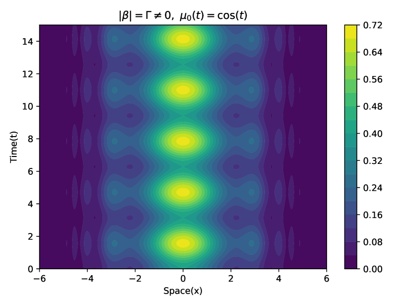
(d)

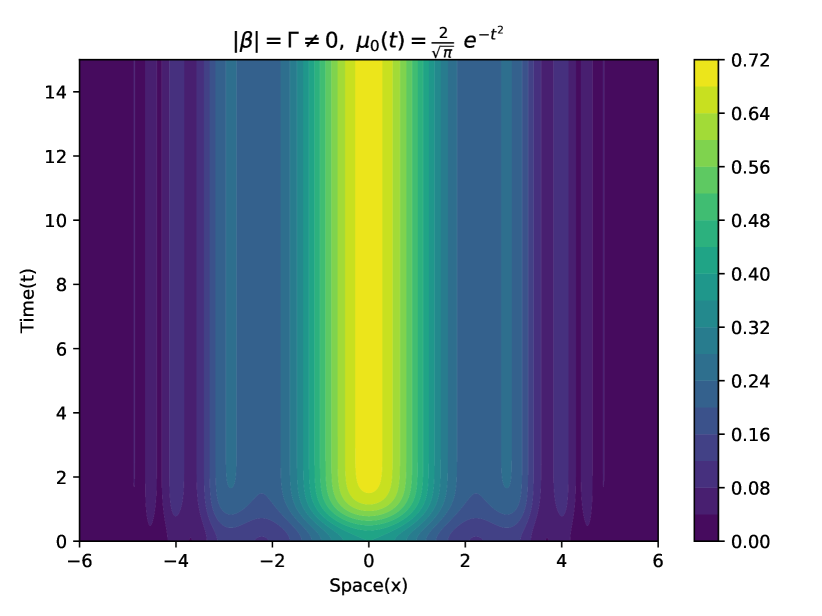
(e)

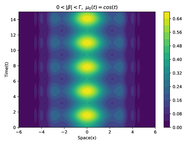
(f)

Figure 2: (Color online) Plot of Power i.e $\Psi^{\dagger}\Psi$ for $V(x)=E^{2}x^{2}$ and the expression of the components of $\Psi$ is given in Eq. (60). Parameters: $W_{1}=W_{2}=1,\theta_{1}=\frac{\pi}{6},\theta_{2}=\frac{2\pi}{3},\theta_{3}=\frac{\pi}{3},Q_{1}=-0.3,Q_{2}=0.1,Q_{3}=0.2,\sigma=-1,E=0.12$. In Fig(a): $\Gamma=|\beta|=0$, Fig(b): $\Gamma=0.5,|\beta|=0.7,\mu_{0}=1$, Fig(c): $\Gamma=|\beta|=0.5,\mu_{0}=1$, Fig(d): $\Gamma=|\beta|=0.5,\mu_{0}(t)=cos(t)$, Fig(e): $\Gamma=|\beta|=0.5,\mu_{0}(t)=\frac{2}{\sqrt{\pi}}e^{-t^{2}}$, Fig(f): $\Gamma=0.5,|\beta|=0.3,\mu_{0}(t)=cos(t)$

VI Systems with Complex $V(x)$

The complex potentials appear in the context of optics through refractive index. The imaginary part of the refractive index is introduced to describe the attenuation of propagating electromagnetic waves in the given material. The ${\cal{PT}}$-symmetric complex potentials have some interesting properties and have been studied extensively in the context of NLSEKonotop1 . We present a few examples of complex confining potential for NLSE with time-dependent LC and BLG, and space-time modulated nonlinear strengths.

The nonlinear strengths $g_{ij}$ may be chosen to be constant, purely time or space dependent or space-time modulated. One notable aspect is that the constant and purely time-dependent $g_{ij}$ may be considered for a complex confining potential, which is not allowed for a real $V(x)$. The function $\theta(x)$ is determined by Eq. (33) for a given $s(x)$ for constant $f(x)$ and $\rho$. Such a freedom to consider a space-dependent $s(x)$ for constant $f$ is absent in Eq. (30) for the case of real potential. There is a freedom in tailoring the nonlinear strengths $g_{ij}$ for a given $f(x)$ by choosing $f_{1}(x)$ and $f_{2}(x)$ appropriately, which may be exploited to construct physically interesting systems.

Scarf II Potential: The ${\cal{PT}}$-symmetric Scarf II complex potential has the form,

$$V(x)=-\frac{V^{2}}{9}sech^{2}(x)-iVsech(x)\tanh(x)$$ (61)

The analytic and numerical solutions of one component NLSE with $V(x)$ has been discussed in Ref. Shi ; Musslimani . We consider constant $f(x)=2\sigma$ for which $f_{1}$ and $f_{2}$ may be chosen as constants or space-dependent subject to the condition $f(x)=\frac{1}{2}(f_{1}(x)+f_{2}(x))$. We choose $E=m=-1$ for simplicity and the phase $\theta(x)$ is determined from Eq. (33) as $\theta(x)=\frac{V}{3}\arctan(\sinh(x))$. We have to choose $\sigma<0$ so that Eqs. (24,25) and (32) are consistent leading to the expression $R(x)=\frac{1}{\sqrt{|\sigma|}}\operatorname{sech}(x)$. The solution of Eq.(12) is obtained as,

$$\Phi=W{{|\sigma|}}^{-\frac{1}{2}}\operatorname{sech}(x)e^{i\big{(}{\frac{V}{3}}\arctan(\sinh(x))+t\big{)}},$$ (62)

which describes a soliton. This completes the extension of the result to the NLSE with time-modulated LC and BLG terms, and space-time modulated nonlinear strengths for the Scarf II potential. The expression of the components of $\Psi$ is given below,

$$\psi_{1}(x,t) = \left[W_{1}e^{i\theta_{1}}\cos(\epsilon)-\left\{i|\beta|W_{2}e^{i\left(\theta_{2}-\theta_{3}\right)}-\Gamma W_{1}e^{i\theta_{1}}\right\}\frac{\sin(\epsilon)}{\epsilon_{0}}\right]{{|\sigma|}}^{-\frac{1}{2}}\operatorname{sech}(x)\ e^{i\left({\frac{V}{3}}\arctan(\sinh(x))+t\right)}$$

$$\psi_{2}(x,t) = \left[W_{2}e^{i\theta_{2}}\cos(\epsilon)-\left\{i|\beta|W_{1}e^{i\left(\theta_{1}+\theta_{3}\right)}+\Gamma W_{2}e^{i\theta_{2}}\right\}\frac{\sin(\epsilon)}{\epsilon_{0}}\right]{{|\sigma|}}^{-\frac{1}{2}}\operatorname{sech}(x)\ e^{i\left({\frac{V}{3}}\arctan(\sinh(x))+t\right)}$$ (63)

The qualitative behaviour of the plots for identical $\mu_{0}(t)$ and condition on $\beta,\Gamma$ are the same with that of Figs. 1 and 2. There is no power oscillation for vanishing $\beta,\Gamma$ as seen in Fig. 3(a). The power-oscillation is seen in Fig. 3(b) for constant $\mu_{0}$ and ${|\beta|}>\Gamma$. The solution grows without any upper bound for constant $\mu_{0}$ and ${|\beta|}=\Gamma$ as is evident from Fig. 3.(c). The management of instabilities for ${|\beta|}\leq\Gamma$ by choosing suitable $\mu_{0}(t)$ is shown in Figs. 3(d), 3(e) and 3(f).

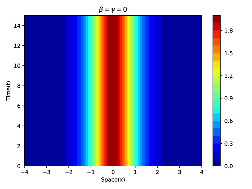
(a)

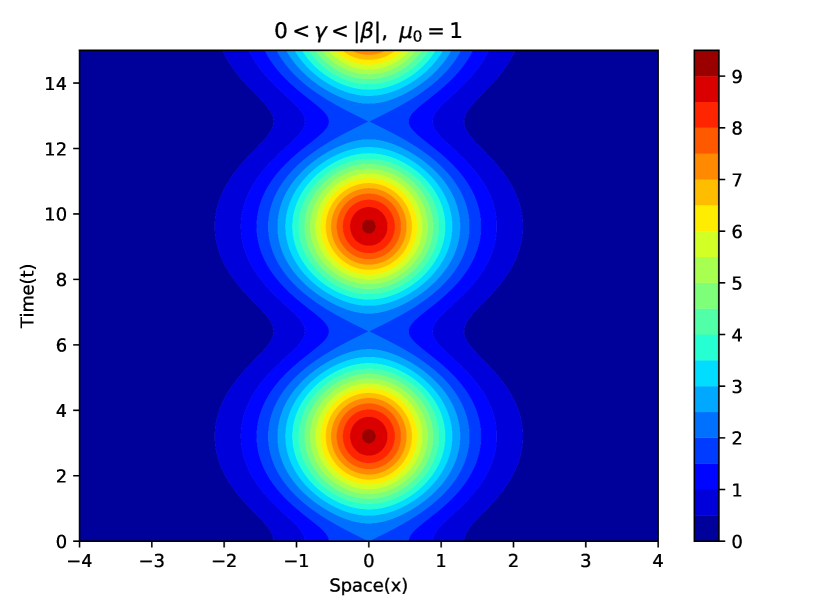
(b)

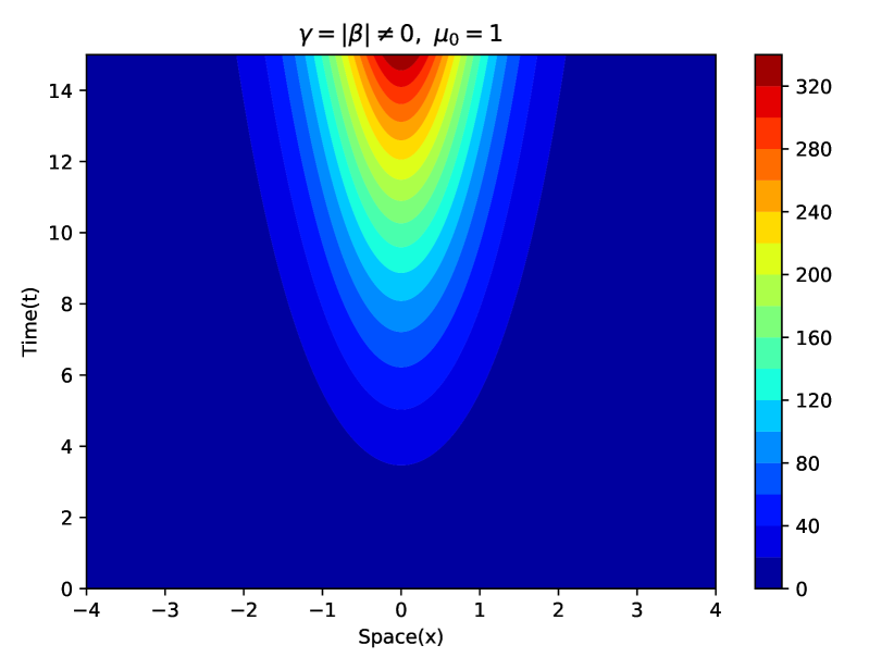
(c)

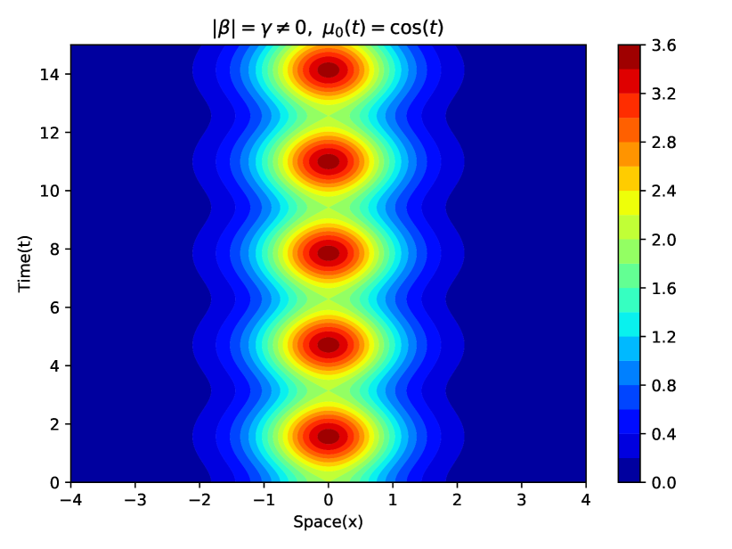
(d)

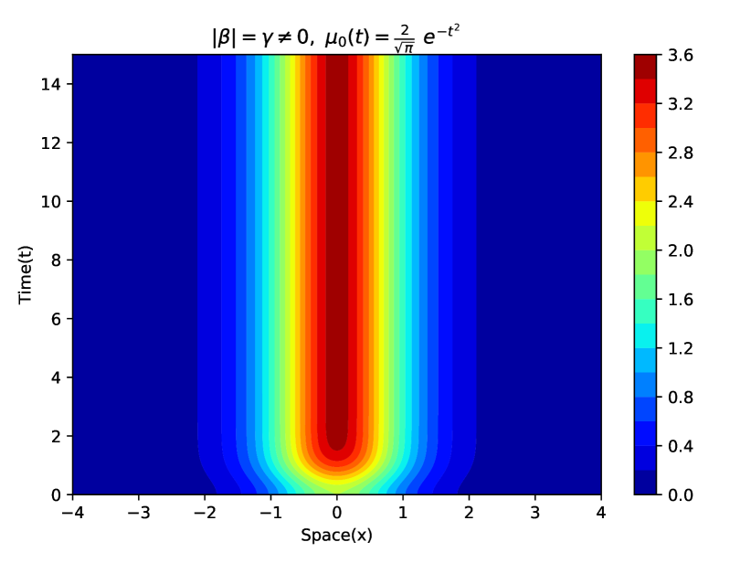
(e)

(f)

Figure 3: (Color online) Plot of Power i.e $\Psi^{\dagger}\Psi$ for Scarf-II potential and the expression of the components of $\Psi$ in Eq. (63). Parameters: $W_{1}=W_{2}=1,\theta_{1}=\frac{\pi}{6},\theta_{2}=\frac{2\pi}{3},\theta_{3}=\frac{\pi}{3},\sigma=-1$. In Fig(a): $\Gamma=|\beta|=0$, Fig(b): $\Gamma=0.5,|\beta|=0.7,\mu_{0}=1$, Fig(c): $\Gamma=|\beta|=0.5,\mu_{0}=1$, Fig(d): $\Gamma=|\beta|=0.5,\mu_{0}(t)=cos(t)$, Fig(e): $\Gamma=|\beta|=0.5,\mu_{0}(t)=\frac{2}{\sqrt{\pi}}e^{-t^{2}}$, Fig(f): $\Gamma=0.5,|\beta|=0.3,\mu_{0}(t)=cos(t)$

Periodic Potential : The ${\cal{PT}}$-symmetric complex potential,

$$V(x)=-\cos^{2}(x)+i\sin(x)$$ (64)

has been considered in Ref. Musslimani in the context of one component NLSE. Following the procedure described above for $E=m=1$ and $\sigma>0$, the solution is determined as,

$$\Phi=W\frac{1}{\sqrt{\sigma}}\sec(x)e^{i\big{(}\sin(x)-t\big{)}}.$$ (65)

We get exact solutions for NLSE with time-modulated LC and BLG terms, and space-time modulated nonlinear strengths for the above periodic potential.

VI.1 Supersymmetry-inspired solution for $f(x)=0$

The techniques of supersymmetric quantum mechanicskhare may be used for $f(x)=0$ to construct a large number of complex potentials for which the NLSE with LC and BLG terms are exactly solvable. The choice $f(x)$=0 can be implemented by fixing $f_{2}(x)=-f_{1}(x)$ and $f_{1},f_{2}$ may be chosen to be either constants or space-dependent. There is a freedom in choosing a large class of space-time modulated $g_{ij}$’s for a given complex $V(x)$. The exact solutions of the NLSE are insensitive to the specific forms of $f_{2}=-f_{1}$ and $G(x,t)$.

The choice $f(x)=0$ reduces Eq.(25) to the linear Schr$\ddot{o}$dinger equation with an effective potential $V_{eff}$:

$$R_{xx}+(E-V_{eff})R=0,\ \ V_{eff}\equiv s(x)+\theta_{x}^{2}.$$ (66)

We may fix $\theta(x)$ in terms of $\tilde{s}(x)$ such that Eqs. (24) and (25) are consistent. We define a function $h(x)$ which is related to $s(x)$ and $\theta(x)$ as follows,

$$s(x)=-h_{x},\ \ \theta(x) = \int^{x}h(x^{\prime})dx^{\prime},$$ (67)

for which $V_{eff}$ has the form of one of the supersymmetric partner potentials,

$$V_{eff}=h^{2}-h_{x}.$$ (68)

The function $h(x)$ is known as superpotential in the context of supersymmetric quantum mechanics. The function $R(x)$ plays the role of eigen-function and $E$ as the energy eigen-value. The zero-energy eigen-function $R_{0}(x)$ has the form,

$$R_{0}(x) = N_{0}\ e^{-\theta(x)},$$ (69)

where $N_{0}$ is a normalization constant. The expression of $R(x)$ for $E\neq 0$ can also be obtained for shape-invariant potentialskhare . We restrict our discussions for $E=0$ in this article and $R_{0}(x)$ can be determined for any $h(x)$ independent of whether it corresponds to shape-invariant potential or not. The factorization of the effective potential $V_{eff}$ as in Eq. (68) ensures exact solution for $R_{0}(x)$. The consistency of Eqs. (24) and (25) fixes the imaginary part and the complex potential has the expression,

$$V(x)=-h_{x}(x)+i\left[h_{x}(x)-2h^{2}(x)\right].$$ (70)

The superpotential corresponding to all the known examples of solvable supersymmetric quantum system may be used to construct complex potential $V(x)$ and the corresponding solution for $R(x)$. The solution $R(x)$ corresponding to these potentials describe localized nonlinear modes. The expression for $\Phi(x,t)$ is determined as,

$$\Phi(x,t)=N_{0}We^{-\theta(x)+i\theta(x)}.$$ (71)

The important point to note is that corresponding to each exactly solved quantum mechanical problem by using supersymmetry, the corresponding superpotential may be used to find a complex potential for which exact localized nonlinear modes are obtained.

We present a few examples to complement the general discussions by including expressions for $h(x),V(x)$ and $\Phi(x)$. Note that $\Phi(x,t)$ is time-independent, since we have chosen $E=0$ for the presentation of results:
Polynomial potential :

$$h(x)=\omega_{0}+\omega_{1}x+\omega_{2}x^{3},\ (\omega_{0},\omega_{1},\omega_{2})\in\ \mathbb{R}^{+},$$

$$V(x)=-(1-i)\left(\omega_{1}+3\omega_{2}x^{2}\right)-2i\left(\omega_{0}+\omega_{1}x+\omega_{2}x^{3}\right)^{2},$$

$$\Phi(x)=N_{0}We^{-(1-i)\left(\omega_{0}x+\frac{\omega_{1}}{2}x^{2}+\frac{\omega_{2}}{4}x^{4}\right)}.$$

The real part of the potential describes a harmonic oscillator, while the imaginary part is a sextic potential. The function $\Phi(x)$ is localized in space even for $\omega_{2}=0$ for which the real part of the potential is constant and the imaginary part is given by an quadratic potential.

Exponential Potential :

$$h(x)=A-Be^{-ax},\ (a,A,B)\in\mathbb{R}^{+},$$

$$V(x)=-Bae^{-ax}+i[2A^{2}-B(a+4A)e^{-ax}+2B^{2}e^{-2ax}],$$

$$\Phi(x)=N_{0}W\ exp[-\frac{B}{a}e^{-ax}-Ax]\ e^{i\big{(}\frac{B}{a}e^{-ax}+Ax\big{)}}.$$

The real part of the $V(x)$ describes a potential well of depth $Ba$ and $\Phi(x)$ is localized in space.

Systems with singular phase: The phase singularity in two and higher dimensional optical systems has interpretation in terms of vortices, wavefront dislocation, etc.berry1 . We present two examples exhibiting phase singularity in one dimension. The first example corresponds to the superpotential for a system describing quantum particle in a box of length $L$:

$$h(x)=-\frac{\pi}{L}cot(\frac{\pi x}{L}),$$

$$V(x)=-\frac{\pi^{2}}{L^{2}}cosec^{2}(\frac{\pi x}{L})+i[\frac{\pi^{2}}{L^{2}}\big{(}1-cot^{2}(\frac{\pi x}{L})\big{)}],$$

$$\Phi(x)=W\ \sqrt{\frac{2}{L}}\ \sin(\frac{\pi x}{L})\ e^{-i\ ln(\sin(\frac{\pi x}{L}))}.$$ (72)

The nonlinear mode is localized within the box and vanishes at the boundary. However, the phase is singular at the boundaries of the box. The second example corresponds to the superpotential of Rosen-Morse potential:

$$h(x)=N\tanh(x),\ N\in\mathbb{R}^{+},$$

$$V(x)=-Nsech^{2}(x)-i[2N^{2}-N(2N+1)sech^{2}(x)],$$

$$\Phi(x)=Wsech^{N}(x)exp[-i\big{(}Nln(sech(x))\big{)}].$$

Both the the real and imaginary parts of $V(x)$ define potential-wells of finite depth. The potential is well-defined on the whole line. The nonlinear mode ‘$\Phi(x)$ is localized in space. The phase of $\Phi(x)$ is singular for ${|x|}\rightarrow\infty$.

VII Discussion and Conclusion

We have investigated exact solvability of a class of vector NLSE with time-modulated LC and BLG terms, and space-time modulated cubic nonlinear terms in presence of an external complex potential. We have taken a two-step approach to find exact solutions. The BLG and LC terms are removed completely through a non-unitary transformation at the cost of modifying the time-modulation of the nonlinear strength. In general, the real-valued nonlinear interaction becomes complex after the non-unitary transformation. Further, the method of non-unitary transformation is applicable only if LC and BLG terms have identical time-modulation. The separation of time and space co-ordinates as well as real and imaginary parts of the equation requires the nonlinear strengths to be time-independent and real-valued. This is achieved by fixing the nonlinear strengths appropriately such that the method of separation works. The time-dependence of the nonlinear strengths is determined in terms of the time-modulation of LC and BLG terms along with an arbitrary function $G(x,t)$, while the space-dependence may be chosen in terms of two arbitrary functions $f_{1}(x),f_{2}(x)$ and $G(x,t)$.

In the second step, the resulting equations are analyzed by using the method of similarity transformation which involves writing the differential equation in a new co-ordinate system and multiplying the amplitude by a space-dependent scale-factor. The treatment for analyzing solvability for real and complex potentials are different. The space-time dependence of the power $P$ is factorised in terms of the product of space-dependent and time-dependent functions. The time-dependence of $P$ solely depends on the form LC and BLG couplings and independent of the specific form of external potential or the strengths of the space-time modulated cubic nonlinearity. However, the space-dependence of $P$ is determined in terms of the choice of the external potential as well as space-modulation of the nonlinear strengths.

We have constructed several examples of exactly solvable models for constant, purely time dependent, purely space dependent and space-time dependent nonlinear-strengths for vanishing external potential. This has been done for constant as well as time-modulated LC and BLG terms. On the other hand, the method employed in this article allows to construct exact solutions for the non-vanishing real potential for purely space dependent or space-time modulated nonlinear strengths. Exact solutions for constant or purely time dependent nonlinear strengths can not be constructed by using the method. The complex external potential allows more flexibility in constructing exactly solvable models. In particular, exactly solvable models for constant, purely time dependent, purely space dependent and space-time dependent nonlinear-strengths, and time-modulated LC and BLG terms are constructed. One interesting result is that exact localized nonlinear modes with spatially constant phase may be obtained for any real $V(x)$ for which the corresponding linear Schr$\ddot{o}$dinger equation is solvable. Further, for the case of complex potential, we have developed a method based on supersymmetric quantum mechanics to construct several exactly solvable models. In fact, corresponding to each exactly solved quantum mechanical problem by using supersymmetry, the corresponding superpotential may be used to find a complex potential for which exact localized nonlinear modes are obtained. We find a few complex potentials for which exact nonlinear modes exhibit singular phases.

A few notable features independent of specific models are the following:

• The exact solutions do not depend at all on the choice of the function $G(x,t)$. The reasons may be attributed to the particular ansatz chosen for the separation of variables, and real and imaginary parts of the differential equation. It is possible that new solutions depending on $G(x,t)$ may be found for the system. Such solution, if exists, have to be found numerically or by different analytical methods.

• The exact solutions do not depend on the specific choices of $f_{1}(x)$ and $f_{2}(x)$, but, on their average $f(x)$. This may again be attributed to the specific ansatz chosen for finding exact solutions. However, analytical and/or numerical methods may be employed to verify whether or not the solutions are insensitive to the choice of specific $f_{1}(x)$ and $f_{2}(x)$.

• The power-oscillation in time is absent for time-independent strength of nonlinear terms. This holds for constant as well as time-modulated LC and BLG terms. The result is to be contrasted with the system considered in Ref. pkg , where power-oscillation is seen for constant LC, BLG and nonlinear strength. There is no contradiction, since the nonlinear term in Eq. (1) for $g_{ij}$ given by Eq. (38) can not be cast in the form $(\psi^{\dagger}M\psi)^{2}$ such that $A$ is pseudo hermitian with respect to $M$. The power oscillation is observed in ref. pkg for constant LC, BLG and nonlinear term whenever $A$ is $M$ pseudo hermitian. Thus, the power-oscillation for constant LC and BLG terms in pkg may be attributed to the specific form of the nonlinear interaction.

• The case $f(x)=0$ for which exact localized nonlinear modes are obtained for real as well as complex potentials is one of the salient features of the class of NLSE considered in this article. The method based on supersymmetric quantum mechanics to construct localized nonlinear modes for complex potential needs to be explored further for its applicability to other types of NLSE with external potential.

The system defined by Eq. (1) is directly relevant in the context of optics. The NLSE has been studied through approximate and/or numerical methods previously for constant nonlinear strengths and constant or specific time-modulated LC and BLG terms. We have given a generic framework in which a class of exact solutions may be found for various combinations of space-time modulated nonlinear strengths, time-modulated LC and BLG terms and external potential. Specific realizations of some of these models in realistic physical scenario may enrich the current understanding on the subject.

VIII Appendix-I: Solutions of a nonlinear equation

We present the solutions of the following equation:

$$u_{\zeta\zeta}+\omega^{2}(\zeta)u-\frac{C^{2}}{u^{3}}-2\sigma u^{3}=0,$$ (73)

where $\sigma$ and $C$ are real constants. We discuss two special cases before embarking on the general solutions:
(I) ${\bf\sigma=0}$: Eq. (73) describes Ermakov-Pinney equation. The general solution is given by,

$$u(\zeta)=\sqrt{v_{1}^{2}+\frac{C^{2}}{W^{2}}v_{2}^{2}},\ W(\zeta)=v_{1}v_{2,\zeta}-v_{2}v_{1,\zeta},$$ (74)

where $v_{1}$, $v_{2}$ are two independent solutions of the equation $v_{\zeta\zeta}+\omega^{2}(\zeta)v=0$ satisfying the initial conditions at $\zeta=\zeta_{0}$: $v_{1}(\zeta_{0})=u(\zeta_{0}),v_{1,\zeta}(\zeta_{0})=u_{\zeta}(\zeta_{0}),v_{2}(\zeta_{0})\neq 0,v_{2,\zeta}(\zeta_{0})=0$. We have used the convention $v_{i,\zeta}=\frac{dv_{i}}{d\zeta},i=1,2$. For constant $\omega$, the choice $v_{1}=\sin(\omega\zeta),v_{2}=\cos(\omega\zeta)$ leads to the periodic solution,

$$u(\zeta) = \sqrt{\sin^{2}(\omega\zeta)+\frac{C^{2}}{w^{2}}\cos^{2}(\omega\zeta)}.$$ (75)

For a periodic $\omega(\zeta)$ with period $T$, we obtain Hill’s equation which has been studied extensively in the literaturehill . The solutions for a generic periodic $\omega(\zeta)$ with the condition $v_{1}(0)=0,v_{1,\zeta}=1,v_{2}(0)=1$ are stable for ${|v_{1}(T)+v_{2,\zeta}(T)|}<2$hill .
(II)  ${\bf C=0}$: In Eq.(73) we replace $\omega^{2}(\zeta)$ with constant $m$ which can take both positive and negative values. This describes a NLSE and it’s solution is well known,

$$u(\zeta) = \sqrt{\frac{m}{\sigma}}\ \sec\big{(}\sqrt{m}\zeta\big{)},\ (m,\sigma)>0$$ (76)

$$= \sqrt{\frac{|m|}{|\sigma|}}\ sech\big{(}\sqrt{|m|}\zeta\big{)},\ (m,\sigma)<0.$$

III.  ${\bf C\neq 0,\sigma\neq 0,\omega^{2}\equiv m=}\textrm{\bf Constant}$: The transformation $u(\zeta)=\sqrt{Q(\zeta)}$ along with a change in the variable from $\zeta$ to $y=\sqrt{|\sigma|}\zeta$ followed by integration transforms Eq. (73) in the following form:

$$Q_{y}^{2}=\operatorname{sgn}(\sigma)\ 4\ (Q-Q_{1})(Q-Q_{2})(Q-Q_{3})$$ (77)

where $Q_{1},Q_{2},Q_{3}$ are the roots of the cubic equation $Q^{3}-\frac{m}{\sigma}Q^{2}+\frac{C_{1}}{\sigma}Q-\frac{C^{2}}{\sigma}=0$, $C_{1}$ is an integration constant and $\operatorname{sgn}(\sigma)$ is the signum function. The expressions for the roots in terms of $\omega,\sigma,C,C_{1}$ are too lengthy and will not be presented here. However, for given values of $Q_{i}$’s in a particular solution, corresponding values of $\omega,\sigma,C,C_{1}$ may be obtained by using the properties of the roots: $Q_{1}Q_{2}Q_{3}=\frac{C^{2}}{\sigma},\ \ Q_{1}Q_{2}+Q_{2}Q_{3}+Q_{1}Q_{3}=\frac{C_{1}}{\sigma},Q_{1}+Q_{2}+Q_{3}=\frac{m}{\sigma}$. The real solutions of Eq. (77) satisfy $(Q-Q_{1})(Q-Q_{2})(Q-Q_{3})\geq 0$ for $\sigma>0$, while $(Q-Q_{1})(Q-Q_{2})(Q-Q_{3})\geq 0$ for $\sigma<0$. The finite and stable solutions of Eq.(77) are presented below based on boundedness of the solution $Q$ in terms $Q_{i}$. A particular ordering among thee roots are considered for presentation of the results following the discussions in Ref. Beitia :
(a) ${\bf\sigma>0,0<Q_{1}\leq Q\leq Q_{2}<Q_{3}}$ : The solution of the Eq.(77) reads,

$$Q=Q_{1}+(Q_{2}-Q_{1})sn^{2}[\lambda y,r],$$ (78)

where $\lambda=\sqrt{Q_{3}-Q_{1}}$ and $r^{2}={\frac{Q_{2}-Q_{1}}{Q_{3}-Q_{1}}}$. The solution can be expressed in terms of hyperbolic function in the limit of $Q_{3}\rightarrow Q_{2}$:

$$Q=Q_{1}+(Q_{2}-Q_{1})\tanh^{2}[\lambda y]$$ (79)

(b) ${\bf\sigma>0,0<Q_{1}<Q_{2}<Q_{3}\leq Q}$: The solution of Eq.(77) reads,

$$Q=Q_{1}+\frac{Q_{3}-Q_{1}}{sn^{2}(\lambda y,r)},$$ (80)

where $\lambda^{2}=Q_{3}-Q_{1}$ and $r^{2}=\frac{Q_{2}-Q_{1}}{Q_{3}-Q_{1}}$. The solution reduces to an elementary singular periodic function for $Q_{1}=Q_{2}$, while it gives a singular soliton if $Q_{3}=Q_{2}$.

(c) ${\bf\sigma<0,Q_{1}<0<Q_{2}\leq Q\leq Q_{3}}$: In this case, we get real finite stable solution. The solution for $\sigma<0$ has the form:

$$Q=Q_{3}-(Q_{3}-Q_{2})sn^{2}(\lambda y,r)$$ (81)

where $\lambda^{2}=Q_{3}-Q_{1}$ and $r^{2}=\frac{Q_{3}-Q_{2}}{Q_{3}-Q_{1}}$.

References

- (1) Y. Kivshar and G. P. Agrawal, Optical Solitons: From fibers to Photonic crystals (Academic Press, 2003).
- (2) V. N. Serkin, A. Hasegawa, and T. L. Belyaeva, Non autonomous Solitons in External Potentials, Phys. Rev. Lett. 98, 074102 (2007).
- (3) V. N. Serkin and A. Hasegawa, Novel Soliton Solutions of the Nonlinear Schrödinger Equation Model, Phys. Rev. Lett. 85, 4502 (2000).
- (4) F. Dalfovo, S. Giorgini, L. P. Pitaevskii, and S. Stringari, Theory of Bose-Einstein condensation in trapped gases, Rev. Mod. Phys. 71, 463 (1999).
- (5) P. G. Kevrekidis, D. J. Frantzeskakis, and R. Carretero-Gonzlez, Editors, Emergent Nonlinear Phenomena in Bose-Einstein Con-densates: Theory and Experiment (Springer, Vol. 45, 2008).
- (6) L. P. Pitaevskii and S. Stringari, Bose-Einstein Conden-sation, (Oxford University Press, Oxford, 2003).
- (7) E. Kengne, W. Liu, and B. A. Malomed, Spatiotemporal engineering of matter-wave solitons in Bose–Einstein condensates, Phy. Rep. 899,1 (2021).
- (8) R. K. Dodd, J. C. Eilbeck, J. D. Gibbon, and H. C. Morris, Solitons and nonlinear wave equations (AcademicPress, New York, 1982).
- (9) K. Trulsen and K. B. Dysthe, A modified nonlinear Schrdinger equation for broader bandwidth gravity waves on deep water , Wave motion 24, 281 (1996).
- (10) A. S. Davydov, Solitons in Molecular Systems (Reidel, Dordrecht, 1985).
- (11) N. J. Zabusky and M. D. Kruskal, Interaction of Solitons in a Collisionless Plasma and the Recurrence of Initial States, Phys. Rev. Lett. 15, 240 (1965).
- (12) A. C. Newell, Solitons in Mathematics and Physics (SIAM, Philadelphia, 1985).
- (13) V. E. Zakharov, S. V. Manakov, S. P. Nonikov, and L. P. Pitaevskii, Theory of Solitons (Consultants Bureau, NY, 1984).
- (14) E. Infeld and G. Rowlands, Nonlinear Waves, Solitons and Chaos (Cambridge University Press, Cambridge, 1990).
- (15) C. Sulem and P. L. Sulem, The Nonlinear Schrdinger Equation (Springer-Verlag, New York , 1999).
- (16) J. Bourgain, Global Solutions of Nonlinear Schrdinger Equations (American Mathematical Society, Providence,1999).
- (17) M. J. Ablowitz, B. Prinari, and A. D. Trubatch, Discrete and Continuous Nonlinear Schrödinger Systems (Cambridge University Press, Cambridge, 2004).
- (18) G. L. Lamb, Elements of Soliton Theory (Wiley, 1980).
- (19) V. E. Korepin, N. M. Bogoliubov, and A. G. Izergin, Quantum Inverse Scattering Method and Correlation Functions, (Cambridge University Press, 2010).
- (20) P. K. Ghosh, Conformal symmetry and the nonlinear Schrodinger equation, Phys.Rev. A 65, 012103 (2002).
- (21) P. K. Ghosh, Explosion-implosion duality in the Bose-Einstein condensation, Phys. Lett. A 308, 411 (2003).
- (22) T. Tsurumi and M. Wadati, Collapses of Wavefunctions in Multi-Dimensional Nonlinear Schrdinger Equations under Harmonic Potential, J. Phys. Soc. Japan 66, 3031 (1997); T. Tsurumi and M. Wadati, Instability of Bose-Einstein Condensate Under Magnetic trap 66, 3035 (1997); M. Wadati and T. Tsurumi, Critical number of atoms for the magnetically trapped Bose-Einstein condensate with negative s-wave scattering length, Phys. Lett. A 247, 287 (1998); T. Tsurumi, H. Morise and M. Wadati, Stability of Bose–Einstein condensate confined in traps, Int. Jour. Mod. Phys. B 14, 655 (2000), cond-mat/9912470.
- (23) F. Kh. Abdullaev and J. Garnier, Propagation of matter-wave solitons in periodic and random nonlinear potentials, Phys. Rev. A 72,061605 (2005).
- (24) H. Sakaguchi and B. A. Malomed, Matter-wave solitons in nonlinear optical lattices, Phys. Rev. E 72, 046610 (2005).
- (25) A. V. Carpentier, H. Michinel, M. I. Rodas-Verde, and V. M. Prez-Garcı, Analysis of an atom laser based on the spatial control of the scattering length, Phys. Rev. A 74, 013619 (2006).
- (26) J. Belmonte-Beitia, F. Gngr, and P. J. Torres, Explicit solutions with non-trivial phase of the inhomogeneous coupled two-component NLS system, J. Phys. A: Math. Theor. 53, 015201 (2019).
- (27) M. I. Rodas-Verde, H. Michinel, and V. M. Prez-Garca, Controllable Soliton Emission from a Bose-Einstein Condensate, Phys. Rev. Lett. 95, 153903 (2005).
- (28) G.Theocharis, P. Schmelcher, P. G. Kevrekidis, and D. J. Frantzeskakis ,Matter-wave solitons of collisionally inhomogeneous condensates, Phys. Rev. A 72, 033614 (2005).
- (29) M. A. Porter, P. G. Kevrekidis, B. A. Malomed and D. J. Frantzeskakis, Modulated amplitude waves in collisionally inhomogeneous Bose–Einstein condensates, Physica D 229, 104 (2007).
- (30) H. Saito and M. Ueda, Dynamically stabilized bright solitons in a two-dimensional Bose–Einstein condensate, Phys. Rev. Lett. 90,040403 (2003).
- (31) P. G. Kevrekidis, D. E. Pelinovsky, and A. Stefanov, Nonlinearity management in higher dimensions, J. Phys. A: Math. Gen. 39, 479 (2005).
- (32) V. A. Brazhnyi and V. V. Konotop, Management of matter waves in optical lattices by means of the Feshbach resonance. Phys. Rev. A, 72, 033615 (2005).
- (33) L. Berg, V. K. Mezentsev, J. Juul Rasmussen, P. Leth Christiansen, and Yu. B. Gaididei, Self-guiding light in layered nonlinear media, Opt. Lett. 25, 1037 (2000).
- (34) I. Towers and B.A. Malomed, Stable(2+1) dimensional solitons in a layered medium with sign-alternating Kerr nonlionearity, J. Opt. Soc. Am. 19, 537 (2002).
- (35) P. G. Kevrekidis, G. Theocharis, D. J. Frantzeskakis, and B. A. Malomed, Feshbach Resonance Management for Bose-Einstein Condensates, Phys. Rev. Lett. 90, 230401 (2003).
- (36) F. Kh. Abdullaev, A. M. Kamchatnov, V. V. Konotop, and V. A. Brazhnyi, Adiabatic dynamics of periodic waves in Bose-Einstein condensate with timedependent atomic scattering length, Phys. Rev. Lett. 90, 230402 (2003).
- (37) V. M. Prez-Garcı, V. V. Konotop, and V. A. Brazhnyi, Feshbach Resonance Induced Shock Waves in Bose-Einstein Condensates, Phys. Rev. Lett. 92, 220403 (2004).
- (38) F. Kh. Abdullaev, J. G. Caputo, R. A. Kraenkel, and B. A. Malomed, Controlling collapse in Bose-Einstein condensates by temporal modulation of the scattering length, Phys. Rev. A 67, 013605 (2003).
- (39) G.D. Montesinos, V.M. Prez-Garci, and P.J. Torres, Stabilization of solitons of the multidimensional nonlinear Schrdinger equation: matter-wave breathers, Phys. D 191, 193 (2004).
- (40) A. Itin, T. Morishita, and S. Watanabe, Reexamination of dynamical stabilization of matter-wave solitons, Phys. Rev. A 74, 033613 (2006).
- (41) V. V. Konotop and P. Pacciani, Collapse of Solutions of the Nonlinear Schrödinger Equation with a Time-Dependent Nonlinearity: Application to Bose–Einstein Condensates, Physical Review Letters 94, 240405 (2005).
- (42) C. M. Bender and S. Boettcher, Real Spectra in Non-Hermitian Hamiltonians Having PT-Symmetry, Phys.Rev.Lett. 80, 5243 (1998).
- (43) V. V. Konotop, J. Yang, and D. A. Zezyulin, Nonlinear waves in PT-symmetric systems, Rev. Mod. Phys. 88, 035002 (2016).
- (44) Z. Shi, X. Jiang, X. Zhu, and H. Li, Bright spatial solitons in defocusing Kerr media with PT-symmetric potentials, Phys. Rev. A 84, 053855 (2011).
- (45) O. Rosas-Ortiz and S. Cruz y Cruz, Superpositions of bright and dark solitons supporting the creation of balanced gain-and-loss optical potentials, Math Meth Appl Sci. 1-12 (2020).
- (46) O. Rosas-Ortiz, O Castanos and D. Schuch, New supersymmetry-generated complex potentials with real spectra, J. Phys. A: Math. Theor. 48 (2015).
- (47) S. Cruz y Cruz, A. Romero-Osnaya and O. Rosas-Ortiz, Balanced Gain-and-Loss Optical Waveguides: Exact Solutions for Guided Modes in Susy-QM, Symmetry-Basel 13 (2021).
- (48) B. Midya and R. Roychoudhury, Nonlinear localized modes in PT-symmetric Rosen-Morse potential wells, Phys. Rev. A 87, 045803 (2013).
- (49) B. Midya and R. Roychoudhury, Nonlinear localized modes in PT-symmetric optical media with competing gainand loss, Annals of Physics 341, 12 (2014).
- (50) Z. H. Musslimani, K. G. Makris, R. El-Ganainy, and D. N. Christodoulides, Optical Solitons in PT Periodic Potentials, Phys. Rev. Lett. 100, 030402 (2008).
- (51) M. J. Ablowitz and Z. H. Musslimani, Integrable Nonlocal Nonlinear Schrdinger Equation, Phys. Rev. Lett. 110, 064105 (2013).
- (52) D. Sinha and P. K. Ghosh, Integrable nonlocal vector nonlinear Schrdinger equation with self-induced parity-time-symmetric potential, Phys. Lett. A 381, 124 (2017).
- (53) D. Sinha and P. K. Ghosh, On Symmetries and Exact Solutions of a Class of Non-local Non-linear Schrdinger Equations with Self-induced PT -symmetric Potential, Phys. Rev. E 91, 042908 (2015).
- (54) M. J. Ablowitz and Z. H. Musslimani, Integrable nonlocal nonlinear equations, Studies in Applied Mathematics 139, 7 (2017).
- (55) V. S. Gerdjikov and A. Saxena, Complete integrability of nonlocal nonlinear Schrdinger equation, J. Math. Phys. 58, 013502 (2017).
- (56) P K Ghosh, Classical Hamiltonian Systems with Balanced loss and gain, J. Phys.: Conf. Ser. 2038, 012012 (2021).
- (57) S. V. Suchkov, B. A. Malomed, S. V. Dmitriev, and Y. S. Kivshar, Solitons in a chain of parity-time-invariant dimers, Physical Review E 84, 046609 (2011).
- (58) Yu. V. Bludov, R. Driben, V. V. Konotop, and B. A. Malomed, Instabilities, Solitons and rogue waves in PT-coupled nonlinear waveguides, J. Opt. 15, 064010 (2013).
- (59) I. V. Barashenkov, S. V. Suchkov, A. A. Sukhorukov, S. V. Dmitriev, and Y. S. Kivshar, Breathers in PT -symmetric optical couplers, Physical Review A 86, 053809 (2012).
- (60) R. Driben, and B. A. Malomed, Stability of solitons in parity-time-symmetric couplers, Opt. Lett. 36, 4323 (2011).
- (61) Yu. V. Bludov, V. V. Konotop, and B. A. Malomed, Stable dark solitons in PT-symmetric dual-core waveguides, Phys. Rev. A 87, 013816 (2013).
- (62) R. Driben, and B. A. Malomed, Stabilization of solitons in PT models with supersymmetry by periodic management, EPL 96, 51001 (2011).
- (63) C. Kharif, E. Pelinovsky, and A. Slunyaev, Rogue waves in the ocean (Springer, Heidelberg, 2009).
- (64) P. K. Ghosh, Constructing Solvable Models of Vector Non-linear Schrdinger Equation with Balanced Loss and Gain via Non-unitary transformation, Phys. Lett. A 402, 127361 (2021).
- (65) F. Kh. Abdullaev, V. V. Konotop, and V. S. Shchesnovich, Linear and nonlinear Zeno effects in an optical coupler, Phys. Rev. A 83, 043811 (2011).
- (66) F. Kh. Abdullaev, V. V. Konotop, M. gren and M. P. Sørensen, Zeno effect and switching of solitons in nonlinear couplers, Opt. Lett. 36, 4566 (2011).
- (67) N. V. Alexeeva, I. V. Barashenkov, A. A. Sukhorukov, and Y. S. Kivshar, Optical solitons in PT-symmetric nonlinear couplers with gain and loss, Phys. Rev. A 85, 063837 (2012).
- (68) F. Cooper, A. Khare, and U. Sukhatme, Supersymmetry and Quantum Mechanics, Phys. Rept. 251, 267 (1995).
- (69) R. El-Ganainy, K. G. Makris, D. N. Christodoulides, and Z. H. Musslimani, Theory of coupled optical PT-symmetric structures, Opt. Lett. 32, 2632 (2007).
- (70) K. G. Markis, R. El-Ganainy, D. N. Christodoulides, and Z. H. Musslimani, Beam Dynamics in PT Symmetric Optical Lattices, Phys. Rev. Lett 100, 103904 (2008).
- (71) S. V. Manakov, On the theory of two-dimensional stationary self-focusing of electromagnetic waves, Soviet Journal of Experimental and Theoretical Physics 38, 248 (1974).
- (72) V. E Zakharov and A. B. Shabat, Exact theory of two-dimensional self-focusing and one-dimensional Self-modulation of waves in nonlinear media, Zh. Eksp. Teor. Fiz. 61, 118 (1971).
- (73) E. Pinney, The nonlinear differential equation , Proceedings of the American Mathematical Society 1, 681 (1950).
- (74) J. Belmonte-Beitia, V. M. Prez-Garci, V. Vekslerchik, and V. V. Konotop, Localized nonlinear waves in systems with time and space-modulated nonlinearities, Phys. Rev. Lett. 100, 164102 (2008).
- (75) V. I. Arnold, Mathematical Methods of Classical Mechanics, Second Edition ( Springer-Verlag, New York, 1989 ).
- (76) M. Berry, Geometry of phase and polarization singularities, illustrated by edge diffraction and the tides, Second international conference on Singular Optics (Optical Vortices): Fundamentals and applications’ SPIE 4403 (Bellingham Washington), 1 (2001).