Generalized Adiabatic Impulse Approximation

Abstract

Non-adiabatic transitions in multilevel systems appear in various fields of physics, but it is not easy to analyze their dynamics in general. In this paper, we propose to extend the adiabatic impulse approximation to multilevel systems. This approximation method is shown to be equivalent to a series of unitary evolutions and facilitates to evaluate the dynamics numerically. In particular, we analyze the dynamics of the Landau–Zener grid model and the multilevel Landau–Zener–Stückelberg–Majorana interference model, and confirm that the results are in good agreement with the exact dynamics evaluated numerically. We also derive the conditions for destructive interference to occur in the multilevel system.

I Introduction

The adiabatic approximation is a well-known approximation technique in quantum mechanics. According to the approximation, the state at any time can be regarded as the $n$th instantaneous eigenstate of the slowly varying time-dependent Hamiltonian if the initial state has been prepared in the $n$th eigenstate of the initial Hamiltonian Born and Fock (1928); Kato (1950); Messiah (1962). This adiabatic approximation has been used in various fields of physics: quantum adiabatic computation Albash and Lidar (2018); Barends et al. (2016) and quantum control Král et al. (2007). If the Hamiltonian changes but not slowly enough, the adiabatic approximation breaks down and transitions between instantaneous eigenstates occur. Such transitions are called non-adiabatic transitions, and the Landau–Zener (LZ) model is known as the simplest and useful model of the non-adiabatic transition in the time-dependent two-level system. Its Hamiltonian has diagonal elements that depend linearly on time, while off-diagonal elements are time-independent Landau (1932); Zener (1932); Stückelberg (1932); Majorana (1932). The dynamics of such non-adiabatic transitions has attracted much attention in various fields and physical systems: quantum information science Quintana et al. (2013); Matityahu et al. (2019), chemical physics Nitzan (2006), atomic physics Salger et al. (2007); Troiani et al. (2017); Zhang et al. (2018); Niranjan et al. (2020), circuit-QED system Chiorescu et al. (2004); Wallraff et al. (2004), ultracold atom system Köhler et al. (2006), and quantum dot system Petta et al. (2010). In general, however, solving the Schrödinger equation for the time-dependent multilevel system is difficult. Therefore, various approximations, including adiabatic approximation, have been adopted to analyze the dynamics. In particular, the adiabatic impulse approximation (AIA) is known as a method that enables us to treat the dynamics analytically Kayanuma (1997); Shevchenko et al. (2010). This is an approximation under which the system evolves adiabatically except when the energy gap becomes small and non-adiabatic transition occurs instantaneously. Since it requires information on instantaneous eigenvalues, this approximation can only be used for relatively small systems such as two- and three-level systems Niranjan et al. (2020); Ostrovsky et al. (2007).

A general method to analytically approximate the dynamics of a multilevel system has not been known so far. On the other hand, there are physical systems with many levels in which non-adiabatic transitions between them play important roles. One of them is known as the multilevel LZ model, in which the diagonal elements of the Hamiltonian depend linearly on time, and the off-diagonal elements are independent of time. Another important example is the multilevel Landau–Zener–Stückelberg–Majorana (LZSM) interference model, in which the diagonal elements of the Hamiltonian are periodic functions of time, while the off-diagonal elements are constants. These models are realizations of such physical systems as Rydberg atom systems Førre and Hansen (2003); Harmin and Price (1994); Harmin (1997), circuit QED systems Werther et al. (2019); Sun et al. (2012); Huang and Zhao (2018); Malla and Raikh (2018); Keeling and Gurarie (2008); Lidal and Danon (2020); Wang et al. (2021); Zheng et al. (2021); Satanin et al. (2012); Du and Yu (2010); Neilinger et al. (2016); Gramajo et al. (2019); Bonifacio et al. (2020); Parafilo and Kiselev (2018), quantum dot systems Forster et al. (2014); Shevchenko et al. (2018); Mi et al. (2018); Petta et al. (2010); Danon and Rudner (2014); Ribeiro et al. (2013); Stehlik et al. (2014, 2016); Pasek et al. (2018), and many-body spin systems Sinitsyn (2013); Wang et al. (2008); Ostrovsky and Volkov (2006). It is thus of essential importance to have appropriate methods to analyze these models.

In this paper, we propose a generalization of AIA (generalized AIA, GAIA) where the scope of AIA is extended to general multilevel systems. For this purpose, we use the idea of exact WKB analysis of previous studies Aoki et al. (2002); Shimada and Shudo (2020). We will show that the idea leads to a succession of local unitary transitions and see that the result is an extension of the conventional AIA. We also illustrate that GAIA can be used for situations where the applicability conditions of previous studies are not necessarily met.

The structure of this paper is as follows. In Sec. II, we review the derivation of the S-matrix within the framework of exact-WKB analysis. In Sec. III, we extend the idea of AIA to the LZ grid model (GAIA) and show that the derived S-matrix agrees well with numerical calculations within a valid parameter region of approximation. In Sec. IV, we derive the S-matrix for the multilevel LZSM interference model by referring to the correspondence between the GAIA derived in Sec. III and previous studies. We show that the results agree with numerical calculations within a valid parameter region of approximation. We also derive the conditions for destructive interference. Finally, a short summary is given in Sec. V.

II review : Exact WKB analysis for three-level LZ model

In this section, we present a brief review of the exact-WKB analysis for the three-level LZ model in previous studies Aoki et al. (2002); Shimada and Shudo (2020). Consider the following Schrödinger equation ($\hbar=1$):

$$i\frac{\partial}{\partial t}|{\psi(t,\eta)}\rangle= H(t,\eta)|{\psi(t,\eta)}\rangle,$$ (1)

$$H(t,\eta)= \eta\left(\begin{array}[]{ccc}\rho_{1}(t)&0&0\\ 0&\rho_{2}(t)&0\\ 0&0&\rho_{3}(t)\end{array}\right)$$ (5)

$$+\eta^{1/2}\left(\begin{array}[]{ccc}0&b_{12}&b_{13}\\ b_{12}^{\ast}&0&b_{23}\\ b_{13}^{\ast}&b_{23}^{\ast}&0\end{array}\right)$$ (9)

$$=: \eta(H_{0}(t)+\eta^{-1/2}H_{1/2}(t)).$$ (10)

Here $\eta$ (essentially equal to $1/\hbar$) is a large parameter (adiabatic parameter). We endeavor to find the S-matrix whose elements $S_{i,j}$ give the transition amplitudes up to phase between basis states $|{i}\rangle$ and $|{j}\rangle$ from $t=-\infty$ to $t=\infty$: $|S_{i,j}|=|\braket{i}{U(\infty,-\infty)}{j}|$, where $U$ is the time-evolution operator generated by the Hamiltonian (10). For this purpose, we construct a global WKB solution and local WKB solutions around the anti-crossing points and connect them.

To find the global WKB solution, we formally diagonalize the Hamiltonian (10): a unitarily transformed state $|\varphi(t,\eta)\rangle$ from $|\psi(t,\eta)\rangle$, $|{\psi(t,\eta)}\rangle=\left(1+\eta^{-1/2}P_{1/2}(t)\right)\left(1+\eta^{-1}P_{1}(t)\right)\cdots|{\varphi(t,\eta)}\rangle$, satisfies

$$i\frac{\partial}{\partial t}|{\varphi(t,\eta)}\rangle= \eta\left(H_{0}(t)+\eta^{-1}\tilde{H}_{1}(t)+\eta^{-3/2}\tilde{H}_{3/2}(t)+\cdots\right)|{\varphi(t,\eta)}\rangle,$$ (11)

where the matrices $P_{i}(t)$ are defined recursively Aoki et al. (2002) to make each $\tilde{H}_{i}(t)$ diagonal. Then the formal solution of (1) that does not suffer from transitions to other states from state $|j\rangle$, the so-called global WKB solution, reads as

$$|{\psi^{(j)}(t,\eta)}\rangle=\exp\left(-i\eta\int^{t}\rho_{j}(t)dt-i\int^{t}\sum_{k\not=j}\frac{\left|b_{jk}\right|^{2}}{\rho_{j}(t)-\rho_{k}(t)}dt\right)|{j}\rangle+O(\eta^{-1}).$$ (12)

To calculate the S-matrix, we need to introduce normalization phase-factor (diagonal) matrices $N^{(\pm)}$ of the global WKB solution at $t\to\pm\infty$:

$$\left(|{j}\rangle,|{k}\rangle,|{l}\rangle\right)= \left(|{\psi^{(j)}(-\infty,\eta)}\rangle,|{\psi^{(k)}(-\infty,\eta)}\rangle,|{\psi^{(l)}(-\infty,\eta)}\rangle\right)N^{(-)},$$ (13)

$$\left(|{j}\rangle,|{k}\rangle,|{l}\rangle\right)= \left(|{\psi^{(j)}(\infty,\eta)}\rangle,|{\psi^{(k)}(\infty,\eta)}\rangle,|{\psi^{(l)}(\infty,\eta)}\rangle\right)N^{(+)}.$$ (14)

Next, we proceed to find the local WKB solution. Since the Schrödinger equation for the two-level LZ model reduces to the Weber equation, we naively assume that the multilevel system can also be described by the Weber equation in the vicinity of the anti-crossing point, but in reality, a more detailed discussion is needed. For this purpose, we first introduce the notion of turning point and Stokes line: the time $t=\tau$ at which $\rho_{j}(\tau)=\rho_{k}(\tau)$ is satisfied is defined as the turning point of type $(j,k)$. The corresponding Stokes curve is defined as such (complex) $t$ that satisfies the condition

$$\operatorname{Im}\left(-i\int_{\tau}^{t}\left(\rho_{j}(t^{\prime})-\rho_{k}(t^{\prime})\right)dt^{\prime}\right)=0.$$ (15)

It is known that the behavior of the asymptotic series changes when the analytic continuation is made crossing over the Stokes curves, and the behavior of the asymptotic series for second-order differential equations such as the Weber function has been well studied. The matrix that relates behavior of the asymptotic series before and after crossing the Stokes curve is called the connection matrix.

In the three-level LZ model, when we consider a vicinity of a turning point, we can consider the Stokes curve in the vicinity. On the other hand, when discussing the global behavior, it is generally necessary to consider other Stokes curves called “new Stokes curves” Aoki et al. (1994, 1998); Honda et al. (2015). It is, however, known that the new Stokes curves do not contribute to the S-matrix if the following reality condition is satisfied Aoki et al. (2002); Shimada and Shudo (2020):

$$\left(\rho_{1}(t)-\rho_{2}(t)\right)\left(\rho_{2}(t)-\rho_{3}(t)\right)\left(\rho_{3}(t)-\rho_{1}(t)\right)=0\text{ has only real and simple zeros}.$$ (16)

In this paper, we consider the cases which do not violate the reality condition or the cases where we need to consider only the ordinary Stokes curves even if the reality condition is violated. Therefore, we need to consider the connection matrix when crossing the Stokes curve near the turning point on the real axis. We define $t_{j,k}^{[n]}$ as the $n$th turning point of type $(j,k)$ and assume

$$\lambda_{j,k}^{[n]}:=\left.\frac{d}{dt}(\rho_{k}(t)-\rho_{j}(t))\right|_{t=t_{j,k}^{[n]}}>0.$$ (17)

The connection matrix $M_{jk}$ responsible for crossing Stokes curve near the turning point at $t=t_{j,k}^{[n]}$ can be expressed as

$$\left(|{\psi^{(j)}(t,\eta)}\rangle,|{\psi^{(k)}(t,\eta)}\rangle,|{\psi^{(l)}(t,\eta)}\rangle\right)\mapsto \left(|{\psi^{(j)}(t,\eta)}\rangle,|{\psi^{(k)}(t,\eta)}\rangle,|{\psi^{(l)}(t,\eta)}\rangle\right)\begin{pmatrix}p_{jk}^{[n]}&-\alpha_{jk}^{[n],+}&0\\ -\alpha_{jk}^{[n],-}&1&0\\ 0&0&1\end{pmatrix}$$ (18)

$$= :\left(|{\psi^{(j)}(t,\eta)}\rangle,|{\psi^{(k)}(t,\eta)}\rangle,|{\psi^{(l)}(t,\eta)}\rangle\right)M_{jk},$$ (19)

where

$$\alpha_{jk}^{[n],\pm}= (2\eta)^{\kappa_{jk}^{[n]}}\sqrt{\frac{2\pi}{\lambda_{jk}^{[n]}}}\frac{b_{jk}^{\pm}}{\Gamma\left(1+\kappa_{jk}^{[n]}\right)}e^{i\pi(1/2\mp 1)\left(\kappa_{jk}^{[n]}\mp 1/2\right)}\left(\beta_{jk}^{[n]}\right)^{\pm 1}\left(1+O\left(\eta^{-1/2}\right)\right),$$ (20)

$$b_{jk}^{+}= b_{jk},\quad b_{jk}^{-}=b^{\ast}_{jk},\quad\kappa_{jk}^{[n]}=\frac{i\left|b_{jk}\right|^{2}}{\lambda_{j,k}^{[n]}},$$ (21)

$$\beta_{jk}^{[n]}= e^{-i\eta\int_{t_{jk}^{[n]}}^{t_{0}}\left(\rho_{j}\left(t^{\prime}\right)-\rho_{k}\left(t^{\prime}\right)\right)dt^{\prime}}\prod_{\begin{subarray}{c}m=1\\ m\neq n\end{subarray}}^{p}\left(t_{jk}^{[n]}-t_{jk}^{[m]}\right)^{-2\kappa_{jk}^{[m]}}\prod_{\begin{subarray}{c}m=1\\ m\neq n\end{subarray}}^{q}\left(t_{jk}^{[n]}-t_{jl}^{[m]}\right)^{-\kappa_{jl}^{[m]}}\prod_{\begin{subarray}{c}m=1\\ m\neq n\end{subarray}}^{r}\left(t_{jk}^{[n]}-t_{kl}^{[m]}\right)^{\kappa_{kl}^{[m]}}\left(\frac{\lambda_{jk}^{[n]}}{2}\right)^{\kappa_{jk}^{[n]}},$$ (22)

with $p,q$, and $r$ expressing the numbers of times that $\rho_{j}(t)$ and $\rho_{k}(t)$, $\rho_{j}(t)$ and $\rho_{l}(t)$, and $\rho_{k}(t)$ and $\rho_{l}(t)$ cross, respectively. In the case of $\rho_{1}(t)=v_{1}t+a,\rho_{2}(t)=v_{2}t,\rho_{3}(t)=v_{3}t$ where $a>0$ and $b_{3}>b_{2}>b_{1}>0$, the connection matrix is given by Aoki et al. (2002)

$$\left(|{\psi^{(j)}(t,\eta)}\rangle,|{\psi^{(k)}(t,\eta)}\rangle,|{\psi^{(l)}(t,\eta)}\rangle\right)\mapsto \left(|{\psi^{(j)}(t,\eta)}\rangle,|{\psi^{(k)}(t,\eta)}\rangle,|{\psi^{(l)}(t,\eta)}\rangle\right)M_{12}M_{13}M_{23}.$$ (23)

The S-matrix (under AIA) can be represented as

$$S= (N^{(+)})^{-1}M_{12}M_{13}M_{23}N^{(-)}$$ (24)

$$= \left(\begin{array}[]{ccc}e^{i\pi\left(\kappa_{12}+\kappa_{13}\right)}&\alpha_{23}^{-}\alpha_{13}^{+}e^{i\pi\left(2\kappa_{12}-\kappa_{23}\right)}-\alpha_{12}^{+}e^{i\pi\kappa_{23}}&-\alpha_{13}^{+}e^{2i\pi\kappa_{12}}+\alpha_{12}^{+}\alpha_{23}^{+}\\ -\alpha_{12}^{-}e^{i\pi\kappa_{13}}&-\alpha_{12}^{-}\alpha_{23}^{-}\alpha_{13}^{+}e^{i\pi\left(\kappa_{12}-\kappa_{23}\right)}+e^{i\pi\left(\kappa_{12}+\kappa_{23}\right)}&\left(\alpha_{12}^{-}\alpha_{13}^{+}-\alpha_{23}^{+}\right)e^{i\pi\kappa_{12}}\\ -\alpha_{13}^{-}e^{i\pi\left(-\kappa_{12}+\kappa_{23}\right)}&-\alpha_{23}^{-}e^{i\pi\kappa_{13}}&e^{i\pi\left(\kappa_{23}+\kappa_{13}\right)}\end{array}\right).$$ (28)

III Landau–Zener grid model

III.1 GAIA

This section considers the LZ grid model, which is a particular case of multilevel LZ models and has two parallel energy bands that cross over time in the energy diagram. We remark that the discussion in this section is also applicable to the general multilevel LZ model. Consider a $2N$-level system governed by the Hamiltonian

$$H(t)= \eta A+\sqrt{\eta}B,$$

$$A= \operatorname{diag}(-vt+a_{1},\cdots,-vt+a_{N}$$

$$\quad\quad\quad\quad,vt+a_{1},\cdots,vt+a_{N}),$$

$$B= \begin{pmatrix}0&\cdots&0&b_{1,N+1}&\cdots&b_{1,2N}\\ \vdots&\ddots&\vdots&\vdots&\ddots&\vdots\\ 0&\cdots&0&b_{N,N+1}&\cdots&b_{N,2N}\\ b_{1,N+1}^{\ast}&\cdots&b_{N,N+1}^{\ast}&0&\cdots&0\\ \vdots&\ddots&\vdots&\vdots&\ddots&\vdots\\ b_{1,2N}^{\ast}&\cdots&b_{N,2N}^{\ast}&0&\cdots&0\end{pmatrix},$$

where $\eta$ is a large parameter Aoki et al. (2002); Shimada and Shudo (2020), the physical meaning of which will be explained later. $v$ is a ramp parameter, $a_{k}$ are responsible for level spacings, and $b_{ij}$ are couplings between $i$th and $j$th levels.

The LZ grid model has applications in various fields, including atomic physics Harmin and Price (1994); Harmin (1997), quantum information science Sun et al. (2012); Malla and Raikh (2017), and open quantum physics Sinitsyn and Prokof’ev (2003); Garanin et al. (2008); Wubs et al. (2006); Saito et al. (2007); Ashhab (2014). No general method, however, is known to analyze the transition probabilities in the LZ grid model. Approximate methods have been developed for the case where the separation of parallel levels in a band is very small Yurovsky and Ben-Reuven (2001). Besides, there are several arguments against the validity of transition probabilities in the LZ grid model Usuki (1997); Wilkinson and Morgan (2000); Malla and Raikh (2017); Malla et al. (2021).

The S-matrix in this model can be obtained approximately as the following matrix $S$ in the same way as in the discussion in Aoki et al. (2002); Shimada and Shudo (2020):

$$S= \left(\tilde{N}^{(+)}\right)^{-1}\tilde{M}_{1}\cdots\tilde{M}_{2N-2}\tilde{M}_{2N-1}\tilde{N}^{(-)},$$ (29)

$$\tilde{M}_{k}= \prod_{\begin{subarray}{c}j-i=k\\ 1\leq i\leq N,N+1\leq j\leq 2N\end{subarray}}M_{i,j},$$ (30)

$$M_{i,j}= \left(\begin{array}[]{ccccc}I_{i-1}&&&&\\ &p_{i,j}&\cdots&-\alpha_{i,j}^{+}&\\ &\vdots&I_{j-i-1}&\vdots&\\ &-\alpha_{i,j}^{-}&\cdots&1&\\ &&&&I_{2N-j}\end{array}\right),$$ (36)

$$\tilde{N}^{(+)}= \prod_{k=1}^{N}\left(\begin{array}[]{ccccc}I_{N}&&&&\\ &p_{k,N+1}^{-1/2}&&&\\ &&p_{k,N+2}^{-1/2}&&\\ &&&\ddots&\\ &&&&p_{k,2N}^{-1/2}\end{array}\right),$$ (42)

$$\tilde{N}^{(-)}= \prod_{k=N+1}^{2N}\left(\begin{array}[]{ccccc}p_{1,k}^{-1/2}&&&&\\ &p_{2,k}^{-1/2}&&&\\ &&\ddots&&\\ &&&p_{N,k}^{-1/2}&\\ &&&&I_{N}\end{array}\right),$$ (48)

$$p_{i,j}= e^{-2\pi\kappa_{i,j}},\quad\kappa_{i,j}=\frac{\left|b_{i,j}\right|^{2}}{2v},$$ (49)

$$\alpha_{i,j}^{\pm}= \pm\sqrt{1-p_{i,j}}$$ (50)

$$\times e^{\pm i\left(\pi/4+\arg\Gamma\left(1-i\kappa_{i,j}\right)+\arg b_{i,j}\right)}(2\eta)^{\pm i\kappa_{i,j}}\beta_{i,j}^{\pm 1},$$ (51)

$$\beta_{i,j}= (4v)^{-i\kappa_{i,j}}e^{i\frac{\eta}{2}\frac{(a_{j}-a_{i})^{2}}{2v}}\prod_{k=1}^{i-1}p^{1/2}_{k,j}\prod_{l=N+1}^{j-1}p_{i,l}^{-1/2}$$

$$\times e^{-i\left(\sum\limits_{\begin{subarray}{c}k=1\\ k\neq i\end{subarray}}^{N}\kappa_{k,j}\log|a_{k}-a_{i}|+\sum\limits_{\begin{subarray}{c}l=N+1\\ l\neq j\end{subarray}}^{2N}\kappa_{i,l}\log|a_{l}-a_{j}|\right)},$$ (52)

where $I_{n}$ is an $n\times n$ identity matrix and $p_{i,j}$ is called the LZ probability. We note that $M_{i,j}$ is not unitary, and the unitarity of the S-matrix is not manifest. Furthermore, when the off-diagonal elements are large, and the LZ probability is small, the term $p^{-1/2}_{i,j}$ included in $\tilde{N}^{(-)}$ becomes large. Such a term is likely to cause errors in numerical calculations, so this formula would not be suited for numerical calculations for such cases. We also note that the reality condition is not satisfied in this model. The above derivation of the S-matrix, however, is not problematic. This is because the Hamiltonian with $a_{i}$ shifted infinitesimally as $a_{i}+\epsilon_{i}$ for $i<N$ and $a_{i-N}$ shifted infinitesimally as $a_{i-N}+\epsilon_{i}$ for $i>N$, where $\epsilon_{i}\neq\epsilon_{j}$ for all $i,j$, satisfies the reality condition, while it is obvious that the S-matrix varies continuously with respect to $\epsilon_{i}$.

Actually, however, we observe that the above matrix (29) can be transformed into a product of unitary matrices $U_{i,j}$ as follows (GAIA, see Appendix A for its derivation):

$$S= \tilde{U}_{1}\cdots\tilde{U}_{2N-2}\tilde{U}_{2N-1},$$ (53)

$$\tilde{U}_{k}= \prod_{\begin{subarray}{c}j-i=k\\ 1\leq i\leq N<N+1\leq j\leq 2N\end{subarray}}U_{i,j},$$ (54)

$$U_{i,j}= \left(\begin{array}[]{ccccc}I_{i-1}&&&&\\ &p^{1/2}_{i,j}&\cdots&-\tilde{\alpha}_{i,j}^{+}&\\ &\vdots&I_{j-i-1}&\vdots&\\ &-\tilde{\alpha}_{i,j}^{-}&\cdots&p^{1/2}_{i,j}&\\ &&&&I_{2N-j}\end{array}\right),$$ (60)

$$\tilde{\alpha}_{i,j}^{\pm}= \pm\sqrt{1-p_{i,j}}$$ (61)

$$\times e^{\pm i\left(\pi/4+\arg\Gamma\left(1-i\kappa_{i,j}\right)+\arg b_{i,j}\right)}(2\eta)^{\pm i\kappa_{i,j}}\tilde{\beta}_{i,j}^{\pm 1},$$ (62)

$$\tilde{\beta}_{i,j}= (4v)^{-i\kappa_{i,j}}e^{i\frac{\eta}{2}\frac{(a_{j}-a_{i})^{2}}{2v}}$$

$$\times e^{-i\left(\sum\limits_{\begin{subarray}{c}k=1\\ k\neq i\end{subarray}}^{N}\log|a_{k}-a_{i}|^{\kappa_{k,j}}+\sum\limits_{\begin{subarray}{c}l=N+1\\ l\neq j\end{subarray}}^{2N}\log|a_{l}-a_{j}|^{\kappa_{i,l}}\right)}.$$ (63)

Hereafter, we express $\tilde{\alpha}_{i,j}^{\pm}$ as

$$\tilde{\alpha}_{i,j}^{\pm}= \pm\sqrt{1-p_{i,j}}e^{\pm i\theta_{i,j}},$$

$$\theta_{i,j}= \frac{\pi}{4}+\arg\Gamma\left(1-i\kappa_{i,j}\right)+\arg b_{i,j}$$

$$+\frac{\eta}{2}\frac{(a_{j}-a_{i})^{2}}{2v}+\log\left(\frac{2\eta}{4v}\right)^{\kappa_{i,j}}-\Theta_{i,j},$$

$$\Theta_{i,j}= \sum_{\begin{subarray}{c}k=1\\ k\neq i\end{subarray}}^{N}\log|a_{k}-a_{i}|^{\kappa_{k,j}}+\sum_{\begin{subarray}{c}l=N+1\\ l\neq j\end{subarray}}^{2N}\log|a_{l}-a_{j}|^{\kappa_{i,l}}.$$

We note that the above derivation is not a direct generalization of AIA to multilevel systems. However, this formula avoids the difficulty of generalizing the AIA directly to multilevel systems. We also note that the S-matrix described above is sufficient to determine the transition probabilities between the basis states of the matrix. To consider a superposition of these states as an initial state, however, it is necessary to take into account the adiabatic evolutions from the initial time $t=-\infty$ to the first anticrossing and from the last anticrossing to the final time $t=\infty$. We will discuss these points in Sec. III.3.

In addition, this transformation not only makes unitarity clear and calculation simple, but also eliminates the need for a normalization factor in $t\to\pm\infty$. This implies that the formula can be applied to time-periodic systems, for example, which do not have a limit at $t\to\pm\infty$. This will be discussed in Sec. IV.

Now, we consider the physical meaning of $\eta$. Since the diagonal elements of the Hamiltonian contain terms $\pm\eta vt$, we define a dimensionless time parameter $\tau=\sqrt{\eta v}t$ and a dimensionless Hamiltonian $\tilde{H}(\tau)=H/\sqrt{\eta v}$. The diagonal elements of $\tilde{H}$ are of order $O(\eta^{0})$, while the off-diagonal elements become $b_{i,j}/\sqrt{v}$. Therefore, the time interval of anticrossing is $\Delta\tau=O(\sqrt{\eta/v})$, while the time interval in which the LZ transition occurs is $\Delta\tau_{LZ}\sim\max\{1,\sqrt{\kappa_{i,j}}\}/\sqrt{2}$ Shevchenko et al. (2010). If $\eta$ is large enough, $\Delta\tau\gg\Delta\tau_{LZ}$ holds and the LZ transition at each anticrossing can be regarded as independent. This does not mean, however, that the local time evolution $\tilde{U}_{i,j}$ can be written with only local parameters such as $\kappa_{i,j}$ when $\eta$ is sufficiently large. In fact, $\Theta_{i,j}$ contains a non-local contribution, and we will see in the next section that this term makes an essential contribution to the transition probabilities.

III.2 Example

We consider a double quantum dot system to confirm the validity of the S-matrix (54). This system has been experimentally realized and its dynamics has drawn much attention Mi et al. (2018); Ginzel et al. (2020). Various methods have been proposed to derive an approximate solution for the dynamics Yurovsky and Ben-Reuven (2001); Malla and Raikh (2017); Malla et al. (2021).

Here, we consider the Hamiltonian with $N=2$, that is, a four-level system. In the following, we set $b_{13}=b_{24}=\Delta$ and $b_{14}=b_{23}=\gamma$. In this case, the S-matrix reads as follows:

$$S=\left(\begin{array}[]{cccc}\sqrt{p_{14}p_{13}}&0&-\tilde{\alpha}_{13}^{+}&-\sqrt{p_{13}}\tilde{\alpha}_{14}^{+}\\ \tilde{\alpha}_{24}^{+}\tilde{\alpha}_{14}^{-}\sqrt{p_{23}}+\tilde{\alpha}_{23}^{+}\tilde{\alpha}_{13}^{-}\sqrt{p_{14}}&\sqrt{p_{23}p_{24}}&-\tilde{\alpha}_{23}^{+}\sqrt{p_{13}}&-\tilde{\alpha}_{24}^{+}\sqrt{p_{23}p_{14}}-\tilde{\alpha}_{23}^{+}\tilde{\alpha}_{13}^{-}\tilde{\alpha}_{14}^{+}\\ -\tilde{\alpha}_{23}^{-}\tilde{\alpha}_{24}^{+}\tilde{\alpha}_{14}^{-}-\tilde{\alpha}_{13}^{-}\sqrt{p_{23}p_{14}}&-\tilde{\alpha}_{23}^{-}\sqrt{p_{24}}&\sqrt{p_{23}p_{13}}&\tilde{\alpha}_{24}^{+}\tilde{\alpha}_{23}^{-}\sqrt{p_{14}}+\tilde{\alpha}_{13}^{-}\tilde{\alpha}_{14}^{+}\sqrt{p_{23}}\\ -\sqrt{p_{24}}\tilde{\alpha}_{14}^{-}&-\tilde{\alpha}^{-}_{24}&0&\sqrt{p_{24}p_{14}}\end{array}\right).$$ (68)

We will compare the approximate solution (68) obtained by GAIA with the solution obtained by numerical calculation with the Python Library QuTiP Johansson et al. (2012, 2013). First, we confirm that GAIA is a good approximation in the region where the approximation that the LZ transitions occur independently is appropriate (Figure 1(a)). In Figure 1(a), the red background region corresponds to the parameter region where the LZ transitions cannot be considered independent $\sqrt{\eta/v}a\not\gg\sqrt{2}\max_{i,j}\{1,\sqrt{\kappa_{i,j}}\}$. Outside of this region, we can see that the numerical solution is in good agreement with (68).

\begin{overpic}[width=170.71652pt]{WKB4_avary_051105_init4_xlog.pdf} \put(19.0,90.0){\Large{(a)}} \end{overpic}

\begin{overpic}[width=170.71652pt]{WKB4_avary_051105_init4_local.pdf} \put(19.0,90.0){\Large{(b)}} \end{overpic}

Figure 1: (a) Numerical results of the transition probability from the initial state $|{4}\rangle$ (closed symbol) and plot of $P_{i4}=|S_{i4}|^{2}$ in (68) obtained by GAIA (open symbol). The parameters are set to $\Delta/\sqrt{v}=0.5$ and $\gamma/\sqrt{v}=1.0$. The parameter region with red background is where the LZ transition cannot be considered independent : $\sqrt{\eta/v}a<10\sqrt{2}\gamma/\sqrt{v}$. As the parameter region is reached where the LZ transitions can be regarded as independent, the numerical and GAIA results coincide. (b) Enlarged view of (a). The gray dashed vertical lines indicate the points where $P_{34}$ (69) vanishes. We used the solver for numerical calculation implemented in the Python Library QuTiP Johansson et al. (2012, 2013).

Next, we look at the contribution from the non-local term $\Theta_{i,j}$. To do so, consider $P_{34}=|S_{34}|^{2}$, which is the probability of measuring $|{3}\rangle$ when the initial state is $|{4}\rangle$ and is given by

$$P_{34}=P_{a}+P_{b}+2\sqrt{P_{a}P_{b}}\cos\biggl{(}2\arg\left(\frac{\Gamma\left(1-i\kappa_{\gamma}\right)}{\Gamma\left(1-i\kappa_{\Delta}\right)}\right)+\frac{\eta a^{2}}{2v}+2\log\left(\frac{\eta a^{2}}{2v}\right)^{-\kappa_{\Delta}+\kappa_{\gamma}}\biggr{)},$$ (69)

where we define $P_{a}:=p_{14}\left(1-p_{24}\right)\left(1-p_{23}\right)$, $P_{b}:=\left(1-p_{14}\right)\left(1-p_{13}\right)p_{23}$, $\kappa_{\Delta}:=\kappa_{13}=\kappa_{24}$, and $\kappa_{\gamma}:=\kappa_{14}=\kappa_{23}$. The $P_{a}$ and $P_{b}$ correspond to the transition probabilities on the paths in Figure 2, and the third term is their interference term. The non-local term $\Theta_{i,j}$ contributes to the last term of the phase. The zeros of (69) are shown in Figure 1(b) as gray dashed lines. We can see that the zeros of (69) and the zeros of the transition probabilities calculated numerically are in good agreement. This result shows that even in the parameter region where the LZ transitions can be regarded as independent, the non-local terms make an essential contribution.

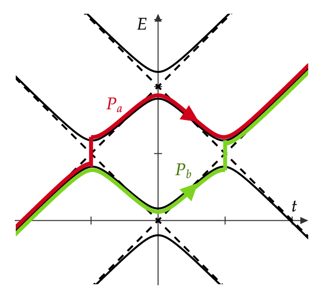
Figure 2: Paths corresponding to $P_{a}$ and $P_{b}$. The third term of (69) results from interference of these paths.

III.3 Comparison with AIA

In this subsection, we investigate the relationship between AIA, an approximation method that has been used so far, and GAIA proposed here. There are two types of AIAs: those using energy basis $|{\epsilon_{i}(t)}\rangle$ Shevchenko et al. (2010); Niranjan et al. (2020) and those using diabatic basis $|{i}\rangle$ Kayanuma (1997); Ostrovsky et al. (2007). Both approximation methods use instantaneous eigenvalues to describe the adiabatic time evolution, which has a disadvantage of being difficult to compute analytically for multilevel systems. Here, we consider a formulation using diabatic basis. In the following, for simplicity, let $a_{n}=(n-1)a\ (1\leq n\leq N)$. In this case, AIA yields the following S-matrix Kayanuma (1997).

$$S= K_{1}\tilde{G}_{1}\cdots\tilde{G}_{2N-2}K_{2N-1}\tilde{G}_{2N-1}K_{2N},$$ (70)

$$\tilde{G}_{k}= \prod_{\begin{subarray}{c}j-i=k\\ 1\leq i\leq N,N+1\leq j\leq 2N\end{subarray}}G_{i,j},$$ (71)

$$G_{i,j}= \left(\begin{array}[]{ccccc}I_{i-1}&&&&\\ &p_{i,j}^{1/2}&\cdots&-\hat{\alpha}^{+}_{i,j}&\\ &\vdots&I_{j-i-1}&\vdots&\\ &-\hat{\alpha}^{-}_{i,j}&\cdots&p_{i,j}^{1/2}&\\ &&&&I_{2N-j}\end{array}\right),$$ (77)

$$K_{k}= e^{-i\int_{t_{k-1}}^{t_{k}}dt\operatorname{diag}\left(E_{1}(t),E_{2}(t),\cdots,E_{2N}(t)\right)},$$ (78)

$$\hat{\alpha}^{\pm}_{i,j}= \pm(1-p_{i,j})^{1/2}e^{\pm i\varphi_{i,j}},$$ (79)

$$\varphi_{i,j}= \frac{\pi}{4}+\kappa_{i,j}(\ln\kappa_{i,j}-1)+\arg\Gamma(1-i\kappa_{i,j}),$$ (80)

where $t_{k}$ stands for the $(2N-k)$th anticrossing time and $E_{i}(t)$, which is related to $i$th diagonal element $H_{ii}(t)$ of Hamiltonian, is the instantaneous eigenvalue $\epsilon_{n}(t)$ in the time interval $[t_{k},t_{k-1}]$ (Figure 3): for example, for $1\leq i\leq N$

$$E_{i}(t)=\begin{dcases}\epsilon_{N+i}(t)&t\leq t_{2N-i}\\ \epsilon_{N-k+2i-1}(t)&t_{2N-k}\leq t\leq t_{2N-k-1}\\ &(k=i,\cdots,i+N-2)\\ \epsilon_{i}(t)&t_{N+i-1}<t\end{dcases},$$ (81)

and for $N+1\leq i\leq 2N$

$$E_{i}(t)= \begin{dcases}\epsilon_{i-N}(t)&t\leq t_{i-1}\\ \epsilon_{2i-l-N}(t)&t_{l}\leq t\leq t_{l-1}\\ &(l=i+1-N,\cdots,i-1)\\ \epsilon_{i}(t)&t_{l-N}<t\end{dcases}.$$ (82)

The S-matrix (70) maps one transition amplitude to one path in the energy diagram (Figure 3). For example, if we specify a path as $(t_{I},t_{F};E_{i})$, then for a path

$$(t_{I},t_{2N-1};E_{i_{1}}) \to(t_{2N-1},t_{2N-2};E_{i_{2}})\to\cdots\to(t_{1},t_{F};E_{i_{2N}}),$$

a transition amplitude

$$e^{-i\int^{t_{F}}_{t_{1}}dtE_{i_{2N}}(t)}\cdots(G_{i_{2},i_{3}})_{i_{3},i_{2}}e^{-i\int^{t_{2N-2}}_{t_{2N-1}}dtE_{i_{2}}(t)}(G_{i_{1},i_{2}})_{i_{2},i_{1}}e^{-i\int^{t_{2N-1}}_{t_{I}}dtE_{i_{1}}(t)}$$ (83)

is selected, where $t_{I}$ and $t_{F}$ are initial and final times. Then, before and after an anticrossing, we can rewrite the amplitude as

$$e^{-i\int^{t_{2N-k-2}}_{t_{2N-k-1}}dtE_{i_{k+2}}(t)}(G_{i_{k+1},i_{k+2}})_{i_{k+2},i_{k+1}}e^{-i\int^{t_{2N-k-1}}_{t_{2N-k}}dtE_{i_{k+1}}(t)}$$

$$= e^{-i\int^{t_{2N-k-2}}_{t_{R}}dtE_{i_{k+2}}(t)}\bigl{(}(G_{i_{k+1},i_{k+2}})_{i_{k+2},i_{k+1}}e^{-i\int^{t_{2N-k-1}}_{t_{R}}dt(E_{i_{k+1}}(t)-E_{i_{k+2}}(t))}\bigr{)}e^{-i\int^{t_{R}}_{t_{2N-k}}dtE_{i_{k+1}}(t)},$$ (84)

where $t_{R}$ is an arbitrary time. Using this transformation, the S-matrix (70) can be transformed as follows:

$$S= K^{\prime}_{1}\tilde{G}^{\prime}_{1}\cdots\tilde{G}^{\prime}_{2N-2}\tilde{G}^{\prime}_{2N-1}K^{\prime}_{2N},$$ (85)

$$\tilde{G}^{\prime}_{k}= \prod_{\begin{subarray}{c}j-i=k\\ 1\leq i\leq N,N+1\leq j\leq 2N\end{subarray}}G_{i,j}^{(k)},$$ (86)

$$G_{i,j}^{(k)}= \left(\begin{array}[]{ccccc}I_{i-1}&&&&\\ &p_{i,j}^{1/2}&\cdots&-\hat{\tilde{\alpha}}^{(k)+}_{i,j}&\\ &\vdots&I_{j-i-1}&\vdots&\\ &-\hat{\tilde{\alpha}}^{(k)-}_{i,j}&\cdots&p_{i,j}^{1/2}&\\ &&&&I_{2N-j}\end{array}\right),$$ (92)

$$\hat{\tilde{\alpha}}^{(k)\pm}_{i,j}= \pm(1-p_{i,j})^{1/2}e^{\pm i\tilde{\varphi}^{(k)}_{i,j}},$$ (93)

$$\tilde{\varphi}^{(k)}_{i,j}= \frac{\pi}{4}+\kappa_{i,j}(\ln\kappa_{i,j}-1)+\arg\Gamma(1-i\kappa_{i,j})$$ (94)

$$+\int_{t_{R}}^{t_{k}}dt(E_{i}(t)-E_{j}(t)),$$ (95)

$$K_{1}^{\prime}= e^{-i\int^{t_{F}}_{t_{R}}dt\operatorname{diag}(E_{1}(t),E_{2}(t),\cdots,E_{2N}(t))},$$ (96)

$$K_{2N}^{\prime}= e^{-i\int^{t_{R}}_{t_{I}}dt\operatorname{diag}(E_{1}(t),E_{2}(t),\cdots,E_{2N}(t))}.$$ (97)

We note here that the contribution from $t_{R}$ can be neglected since it offsets the other terms. If we ignore $t_{R}$, we can see that the S-matrix (85) is similar to the S-matrix of GAIA (54). As we mentioned before, when computing the transition amplitude for the case where the initial state is a superposition of eigenstates, the S-matrix (54) is not correct, and the contribution of $K^{\prime}_{2N}$ and $K^{\prime}_{1}$ in (85) must be taken into account.

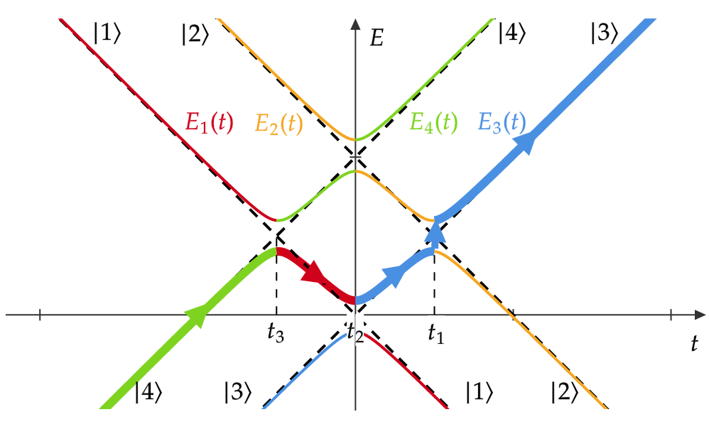
Figure 3: The correspondence between a path and a transition amplitude. The figure shows a path $(t_{I},t_{3};E_{4})\to(t_{3},t_{2};E_{1})\to(t_{2},t_{1};E_{3})\to(t_{1},t_{F};E_{3})$. The time evolution is considered adiabatic at $t\neq t_{i}$ in AIA. If the LZ transition happens at $t=t_{i}$, we multiply the transition amplitude by LZ transition probability. On the other hand, if the LZ transition does not happen at $t=t_{i}$, we multiply the transition amplitude by $\hat{\alpha}^{\pm}$.

It can be seen that the S-matrix (85) obtained in AIA is similar to the previously obtained S-matrix (54). If we perturbatively expand the integral of $E_{i}(t)-E_{j}(t)$ formally, we get

$$\int_{t_{R}}^{t_{k}}dt(E_{i}(t)-E_{j}(t))= \int_{t_{R}}^{t_{k}}dt(H_{ii}(t)-H_{jj}(t))$$

$$+\int_{t_{R}}^{t_{k}}dt\left(\sum_{n=1}^{N}\frac{-\eta|b_{n,j}|^{2}}{H_{jj}(t)-H_{nn}(t)}\right.$$

$$\quad\left.+\sum_{m=N+1}^{2N}\frac{\eta|b_{i,m}|^{2}}{H_{ii}(t)-H_{mm}(t)}\right)$$

$$+O(\eta^{-1})$$

because $H_{ii}(t)\propto\eta$. This perturbation, however, breaks down at the anti-crossing point since we have $H_{nn}(t)-H_{mm}(t)=-2\eta v(t-t_{m-n})\ (1\leq n\leq N,N+1\leq m\leq 2N)$. It can be seen that GAIA successfully avoids the breakdown of the perturbation of AIA. Therefore, the way of obtaining the S-matrix (54) previously is a more general one that extends the AIA to multilevel systems.

IV Multilevel Landau–Zener–Stückelbelg–Majorana Interference Model

IV.1 GAIA

In this section, we consider the multilevel Landau–Zener–Stückelberg–Majorana (LZSM) interference model, which is an extension of the LZSM interference model of two-level systems Shevchenko et al. (2010) and includes, for example, the photon-assisted Landau-Zener model, which is a system of a driven spin and single-mode boson Werther et al. (2019); Sun et al. (2012); Lidal and Danon (2020); Wang et al. (2021); Zheng et al. (2021); Neilinger et al. (2016); Bonifacio et al. (2020). The model is described by the Hamiltonian

$$H(t)= \eta A(t)+\sqrt{\eta}B,$$

$$A(t)= \operatorname{diag}(-\sin(vt)+a_{1},\ldots,-\sin(vt)+a_{N},$$

$$\quad\quad\quad\sin(vt)+a_{1},\ldots,\sin(vt)+a_{N}),$$

$$B= \begin{pmatrix}0&\cdots&0&b_{1,N+1}&\cdots&b_{1,2N}\\ \vdots&\ddots&\vdots&\vdots&\ddots&\vdots\\ 0&\cdots&0&b_{N,N+1}&\cdots&b_{N,2N}\\ b_{1,N+1}^{\ast}&\cdots&b_{N,N+1}^{\ast}&0&\cdots&0\\ \vdots&\ddots&\vdots&\vdots&\ddots&\vdots\\ b_{1,2N}^{\ast}&\cdots&b_{N,2N}^{\ast}&0&\cdots&0\end{pmatrix}.$$

We consider the reality condition, i.e., a condition for the existence of energy gaps without anticrossing Aoki et al. (2002); Shimada and Shudo (2020). The existence of such gaps requires the consideration of new Stokes curves and the discussion in the previous section cannot be used. The reality condition is satisfied when the relation

$$\frac{\eta}{H_{ii}(t)-H_{jj}(t)} =\sum_{m}\frac{1}{\lambda_{i,j,m}\left(t-t_{i,j,m}\right)}$$ (98)

$$\lambda_{i,j,m} =\frac{1}{\eta}\left.\frac{d}{dt}\left(H_{jj}(t)-H_{ii}(t)\right)\right|_{t=t_{i,j,m}}$$ (99)

holds, where $t_{i,j,m}$ stands for the $m$th zero of the denominator (i.e, the time when the $i$th state and the $j$th state cross in the energy diagram for the $m$th time). We note that we do not impose the positivity of $\lambda_{i,j,m}$ here, but we fix $1\leq i\leq N$ and $N+1\leq j\leq 2N$. Hereafter, we impose $\lambda_{i,j,m}\neq 0$ if $b_{i,j}\neq 0$. The condition (98) is always satisfied whenever the left-hand side is analytic (including infinity) except for simple poles on the real $t$. In the multilevel LZSM interference model, indeed, if $|a_{i}-a_{j}|<2\ (1\leq i\leq N,N+1\leq j\leq 2N)$ is satisfied,

$$\frac{\eta}{H_{ii}(t)-H_{jj}(t)}$$ (100)

$$= \sum_{n}\left((-1)^{n}2v\sqrt{1-\frac{(a_{i}-a_{j})^{2}}{4}}\right.$$ (101)

$$\times\left.\left(t+\frac{(-1)^{n}\arcsin\left(\frac{a_{i}-a_{j}}{2}\right)+(n-1)\pi}{v}\right)\right)^{-1}$$ (102)

holds, so the reality condition is satisfied.

Since the instantaneous eigenstates of the Hamiltonian do not coincide with the computational basis at $t=\pm\infty$, the method of calculating the S-matrix in the previous study Aoki et al. (2002); Shimada and Shudo (2020) cannot be used for this model. Formally, $M_{i,j}$ can be obtained, but the normalization factor $\tilde{N}^{(\pm)}$ cannot be obtained. On the other hand, in the previous section, we have seen that the same S-matrix is obtained just by replacing the matrix $M_{i,j}$ with the unitary matrix $U_{i,j}$ and discarding the normalization factors $\tilde{N}^{(\pm)}$. We therefore consider, also in this model, a product of the unitary matrices $U_{i,j,n}$ describing the unitary evolution between $|i\rangle$ and $|j\rangle$ across the $n$th anticrossing, in place of $M_{i,j,n}$ and assume that it represents the S-matrix. Here, the unitary matrix $U_{i,j,n}$ can be written as follows:

$$U_{i,j,n}= \left(\begin{array}[]{ccccc}I_{i-1}&&&&\\ &p^{1/2}_{i,j,n}&\cdots&-\tilde{\alpha}_{i,j,n}^{+}&\\ &\vdots&I_{j-i-1}&\vdots&\\ &-\tilde{\alpha}_{i,j,n}^{-}&\cdots&p^{1/2}_{i,j,n}&\\ &&&&I_{2N-j}\end{array}\right),$$

$$\tilde{\alpha}_{i,j,n}^{\pm}= \pm\operatorname{sgn}(\lambda_{i,j,n})\sqrt{1-p_{i,j,n}}e^{\pm\operatorname{sgn}(\lambda_{i,j,n})i\theta_{i,j,n}},\quad p_{i,j,n}=e^{-2\pi\kappa_{i,j,n}},\quad\kappa_{i,j,n}=\frac{|b_{ij}|^{2}}{|\lambda_{i,j,n}|},$$

$$\theta_{i,j,n}= \frac{\pi}{4}+\arg\Gamma\left(1-i\kappa_{i,j,n}\right)+\arg b_{i,j}+\zeta_{i,j,n}+\log\left(\frac{\eta}{|\lambda_{i,j,n}|}\right)^{\kappa_{i,j,n}}-\Theta_{i,j,n},$$

$$\Theta_{i,j,n}= \log\left(\prod_{\begin{subarray}{c}m=-\infty\\ (m\neq n)\end{subarray}}^{\infty}\left|\lambda_{i,j,m}\left(t_{i,j,n}-t_{i,j,m}\right)\right|^{2\kappa_{i,j,n}}\right.$$

$$\left.\times\prod_{\begin{subarray}{c}m=-\infty\end{subarray}}^{\infty}\left(\prod_{\begin{subarray}{c}k=1\\ k\neq i\end{subarray}}^{N}\left|\lambda_{k,j,m}\left(t_{i,j,n}-t_{k,j,m}\right)\right|^{\kappa_{k,j,m}}\prod_{\begin{subarray}{c}l=N+1\\ l\neq j\end{subarray}}^{2N}\left|\lambda_{i,l,m}\left(t_{i,j,n}-t_{i,l,m}\right)\right|^{\kappa_{i,l,m}}\right)\right),$$

$$\zeta_{i,j,n}= \operatorname{sgn}(\lambda_{i,j,n})\int^{t_{(i,j),n}}(H_{ii}(t,\eta)-H_{jj}(t,\eta))dt.$$

Notice that $\Theta_{i,j,n}$ includes infinite products which, however, can be made simplified:

$$\prod_{\begin{subarray}{c}m=-\infty\end{subarray}}^{\infty}\left|\lambda_{k,j,m}\left(t_{i,j,n}-t_{k,j,m}\right)\right|^{\kappa_{k,j,m}}$$ (103)

$$=\left|\frac{\sin(\frac{v(t_{i,j,n}-t_{k,j,0})}{2})}{\sin(\frac{v(t_{i,j,n}-t_{k,j,1})}{2})}\right|^{\kappa_{k,j,0}}$$ (104)

and

$$\prod_{\begin{subarray}{c}m=-\infty\\ (m\neq n)\end{subarray}}^{\infty}\left|\lambda_{i,j,m}\left(t_{i,j,n}-t_{i,j,m}\right)\right|^{2\kappa_{i,j,n}}$$ (105)

$$= \left|\frac{v}{2\lambda_{i,j,n}\sin(\frac{v(t_{i,j,n}-t_{i,j,n+1})}{2})}\right|^{2\kappa_{i,j,n}}.$$ (106)

In this way, we need only finite products to calculate $\Theta_{i,j,n}$:

$$\Theta_{i,j,n}= \log\left(\left|\frac{v}{2\lambda_{i,j,n}\sin(\frac{v(t_{i,j,n}-t_{i,j,n+1})}{2})}\right|^{2\kappa_{i,j,n}}\right.$$ (107)

$$\left.\times\prod_{\begin{subarray}{c}k=1\\ (k\neq i)\end{subarray}}^{N}\left|\tan\left(\frac{v(t_{i,j,n}-t_{k,j,0})}{2}\right)\right|^{\kappa_{k,j,0}}\prod_{\begin{subarray}{c}l=N+1\\ (l\neq j)\end{subarray}}^{2N}\left|\tan\left(\frac{v(t_{i,j,n}-t_{i,l,0})}{2}\right)\right|^{\kappa_{i,l,0}}\right).$$ (108)

IV.2 Example

We consider a driven system of a spin and a single-mode boson Werther et al. (2019); Sun et al. (2012); Lidal and Danon (2020); Wang et al. (2021); Zheng et al. (2021); Neilinger et al. (2016); Bonifacio et al. (2020), described by the Hamiltonian

$$H(t)= -\eta\sin(vt)\sigma_{z}+\sqrt{\eta}\Delta\sigma_{x}$$ (109)

$$+\eta\Omega b^{\dagger}b+\sqrt{\eta}\gamma\sigma_{x}\left(b+b^{\dagger}\right)$$ (110)

$$=: \eta A(t)+\sqrt{\eta}B$$ (111)

$$A(t)= \operatorname{diag}(-\sin(vt),-\sin(vt)+\Omega,\ldots,$$ (112)

$$\quad\quad\quad\sin(vt),\sin(vt)+\Omega,\ldots)$$ (113)

$$B= \begin{pmatrix}0&0&0&\cdots&\Delta&\gamma&0&\cdots\\ 0&0&0&\cdots&\gamma&\Delta&\sqrt{2}\gamma&\cdots\\ 0&0&0&\cdots&0&\sqrt{2}\gamma&\Delta&\cdots\\ \vdots&\vdots&\vdots&\ddots&\vdots&\vdots&\vdots&\ddots\\ \Delta&\gamma&0&\cdots&0&0&0&\cdots\\ \gamma&\Delta&\sqrt{2}\gamma&\cdots&0&0&0&\cdots\\ 0&\sqrt{2}\gamma&\Delta&\cdots&0&0&0&\cdots\\ \vdots&\vdots&\vdots&\ddots&\vdots&\vdots&\vdots&\ddots\end{pmatrix}.$$ (114)

Figure 4 shows the energy spectrum of the Hamiltonian. In the following numerical calculation, the dimension of the boson Hilbert space is truncated at $N=5$. Since the off-diagonal elements are unbounded, they always violate the condition for GAIA $\Delta\tau\gg\Delta\tau_{LZ}$. However, as long as the probability amplitude at the anticrossing that violates the condition for GAIA is $0$, GAIA is considered reasonable.

\begin{overpic}[width=163.60333pt]{periodical_10_energy_020101.pdf} \put(19.0,90.0){\Large{(a)}} \end{overpic}

\begin{overpic}[width=163.60333pt]{periodical_10_energy_10101.pdf} \put(19.0,90.0){\Large{(b)}} \end{overpic}

Figure 4: Energy spectra of (110) when $\gamma=0.1\sqrt{v}$, $\Delta=0.1\sqrt{v}$, $\eta=10v$, and (a) $\sqrt{\eta/v}a=0.2$ and (b) $\sqrt{\eta/v}a=1.0$. The dimension of the boson Hilbert space is truncated at $5$. In (b), the transition does not occur at times when the energies are in contact because $b_{i,N+i+3}=0$.

\begin{overpic}[width=184.9429pt]{prob_periodical10_0200201_20.pdf} \put(19.0,66.5){\Large{(a)}} \end{overpic}

\begin{overpic}[width=184.9429pt]{prob_periodical10_020101_20.pdf} \put(19.0,66.5){\Large{(b)}} \end{overpic}

\begin{overpic}[width=184.9429pt]{prob_periodical10_100201_20.pdf} \put(19.0,66.5){\Large{(c)}} \end{overpic}

\begin{overpic}[width=184.9429pt]{prob_periodical10_10101_20.pdf} \put(19.0,66.5){\Large{(d)}} \end{overpic}

Figure 5: Time dependence of the transition probability. The parameters are $\Delta=0.1\sqrt{v}$, $\eta=10v$, and (a) $\sqrt{\eta/v}a=0.2,\gamma=0.02\sqrt{v}$, (b) $\sqrt{\eta/v}a=0.2,\gamma=0.1\sqrt{v}$, (c) $\sqrt{\eta/v}a=1.0,\gamma=0.02\sqrt{v}$, and (d) $\sqrt{\eta/v}a=1.0,\gamma=0.1\sqrt{v}$. Solid lines and dashed lines represent the results of numerical calculations, and the dots represent the results of GAIA.

The other condition to be satisfied is the reality condition. In the previous discussion, we explained that the reality condition is satisfied in this model by imposing the condition $|a_{i}-a_{j}|<2$. Since the reality condition is a condition of the anticrossing, even if the condition $|a_{i}-a_{j}|<2$ is not satisfied, GAIA is applicable if $b_{i,j}=0$ (Figure 4(b)).

Because we truncate the dimension of the boson Hilbert space, the transition probabilities can be adequately approximated within a finite number of crossings. In the following, we compare the results of GAIA with the exact results (numerical calculations) when $20$ crossings occur (Figure 5). The initial state is set to be the ground state of the initial Hamiltonian $|{1}\rangle$.

First, we consider the case of $\sqrt{\eta/v}a=0.2$. For example, in the case of $\gamma=0.02\sqrt{v}$, we find that the results agree well with the numerical results within the range of $20$ crossings (Figure 5(a)). On the other hand, in the case of $\gamma=0.1\sqrt{v}$, the numerical results cannot be approximated well because of the large off-diagonal elements (Figure 5(b)). Next, we consider the case of $\sqrt{\eta/v}a=1.0$. In this case, we find that the results agree well with the numerical results in the case not only of $\gamma=0.02\sqrt{v}$ but also of $\gamma=0.1\sqrt{v}$ (Figure 5(c,d)). This can be explained by the fact that the time intervals of the anticrossing become larger, which means that the conditions for GAIA are satisfied. We note that since the dimension of the boson Hilbert space $N$ is finitely truncated in the numerical calculation, the dynamics, especially after the time when the probability amplitude of the $(2N-1)$th excited state is large, is different from the dynamics under the actual Hamiltonian (110).

The interference plays an important role in the periodical model Du and Yu (2010); Bonifacio et al. (2020); Lidal and Danon (2020); Neilinger et al. (2016); Wang et al. (2021). Although the conditions for interference in the two-level system have been studied, the conditions for interference in the multilevel system have not been studied straightforwardly so far. By using the S-matrix here obtained, the conditions for interference can be derived. For example, if the initial state is the ground state, we can derive the condition of destructive interference for the Hamiltonian (110) which means $S_{11}=1$ after $2$ crossings occur. When $2$ crossings occur, the transition amplitude between $|{1}\rangle$ becomes

$$S_{11}= (1-p_{1,N+1})e^{i\left(\theta_{1,N+1,1}+\theta_{1,N+1,2}\right)}$$ (115)

$$+p_{1,N+1}(1-p_{1,N+2})e^{i\left(\theta_{1,N+2,1}+\theta_{1,N+2,2}\right)}$$ (116)

$$+p_{1,N+1}p_{1,N+2}.$$ (117)

If the conditions $\theta_{1,N+1,1}+\theta_{1,N+1,2}=2\mathbb{Z}\pi$ and $\theta_{1,N+2,1}+\theta_{1,N+2,2}=2\mathbb{Z}\pi$ hold, $S_{11}=1$ and a destructive interference occurs (Figure 6). We note that we have truncated the dimension of the boson, but this does not affect the conditions for destructive interference.

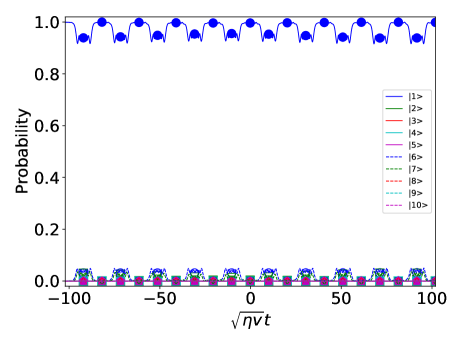
Figure 6: Time evolution when the conditions for destructive interference are satisfied. The parameters are $\Delta=\gamma=0.1\sqrt{v}$, $\sqrt{\eta/v}a=0.2\sqrt{v}$, and $\eta=10.57v$, which are satisfied with (117).

V Conclusion

In this study, we propose a GAIA by improving the S-matrix obtained in previous studies Aoki et al. (2002); Shimada and Shudo (2020) and applied the results to the LZ grid model and the LZSM interference model. The division of the S-matrix into unitary matrices, not only makes numerical calculations easier, but also allows for a physical interpretation. In the LZ grid model, we have investigated the relation between the S-matrix obtained by GAIA and the conventional AIA. In addition, we have analyzed the LZSM interference model, for which the previous methods Aoki et al. (2002); Shimada and Shudo (2020) have difficulties to analyze, and a new condition for interference is obtained.

The present results can be applied to other multilevel LZ model, for which integrability conditions have been studied Sinitsyn and Chernyak (2017); Sinitsyn et al. (2018); Chernyak et al. (2018, 2020a, 2020b); Chernyak and Sinitsyn (2021). We expect that the present method can be used to obtain the necessary condition for integrability. In the integrable multilevel LZ model, crossing three or more levels at a single point were sometimes considered. Since GAIA cannot calculate the S-matrix of such a model, it is necessary to extend the present method. We note that GAIA can describe well the dynamics when non-adiabatic transitions generate interference. We expect that GAIA can be applied to quantum information processing in such a setting Wubs et al. (2007); Deng et al. (2016); Munoz-Bauza et al. (2019).

Appendix A Unitary Decomposition

To express the S matrix as a product of unitary matrices, we define the matrix $\tilde{U}_{k}$ as follows:

$$\tilde{M}_{k}\tilde{N}_{k}^{(-)}= \tilde{N}_{k-1}^{(-)}\tilde{U}_{k},\quad(\tilde{N}_{2N-1}^{(-)}=\tilde{N}^{(-)}),$$ (118)

where

$$\tilde{N}_{k}^{(-)}=\begin{dcases}\operatorname{diag}\Biggl{(}\overbrace{\prod_{l=N+1}^{k+1}p_{1l}^{-1/2},\cdots,\prod_{l=N+1}^{2N}p_{2N-k-1,l}^{-1/2},}^{2N-k-1}\overbrace{\prod_{l=N+1}^{2N}p_{2N-k,l}^{-1/2},\cdots,\prod_{l=N+1}^{2N}p_{Nl}^{-1/2}}^{k-N+1},\\ \quad\quad\quad\vec{I}_{k-N+1},\overbrace{\prod_{l=1}^{1}p_{l,k+2}^{-1/2},\cdots,\prod_{l=1}^{2N-k-1}p_{l,2N}^{-1/2}}^{2N-k-1}\Biggr{)}&(k\geq N)\\ \operatorname{diag}\Biggl{(}\vec{I}_{N-k},\overbrace{\prod_{l=N+1}^{N+1}p_{N-k+1,l}^{-1/2},\cdots,\prod_{l=N+1}^{N+k}p_{N,l}^{-1/2},}^{k}\\ \quad\quad\quad\overbrace{\prod_{l=1}^{N-k}p_{l,N+1}^{-1/2},\cdots,\prod_{l=1}^{N-1}p_{l,N+k}^{-1/2},}^{k}\overbrace{\prod_{l=1}^{N}p_{l,N+k+1}^{-1/2},\cdots\prod_{l=1}^{N}p_{l,2N}^{-1/2}}^{N-k}\Biggr{)}&(k\leq N)\end{dcases},$$ (119)

and we also define

$$\vec{I}_{n}=(\overbrace{1,\cdots,1}^{n}).$$

The matrix $M_{i,j}$ can be transformed using any $X_{i,j},Y_{i,j}\in\mathbb{C}$ as follows:

$$M_{i,j}= \left(\begin{array}[]{ccccc}I_{i-1}&&&&\\ &X^{1/2}_{i,j}&\cdots&0&\\ &\vdots&I_{j-i-1}&\vdots&\\ &0&\cdots&X^{-1/2}_{i,j}Y_{i,j}^{-1}&\\ &&&&I_{2N-j}\end{array}\right)$$

$$\times\left(\begin{array}[]{ccccc}I_{i-1}&&&&\\ &p_{i,j}X_{i,j}^{-1}&\cdots&-\alpha_{i,j}^{+}Y^{-1}_{i,j}&\\ &\vdots&I_{j-i-1}&\vdots&\\ &-\alpha_{i,j}^{-}Y_{i,j}&\cdots&X_{i,j}&\\ &&&&I_{2N-j}\end{array}\right)\left(\begin{array}[]{ccccc}I_{i-1}&&&&\\ &X_{i,j}^{1/2}&\cdots&0&\\ &\vdots&I_{j-i-1}&\vdots&\\ &0&\cdots&X^{-1/2}_{i,j}Y_{i,j}&\\ &&&&I_{2N-j}\end{array}\right)$$

$$=: M_{i,j}^{(-)}\tilde{U}_{i,j}M_{i,j}^{(+)}.$$

Hereafter, we define $X_{i,j}=p_{i,j}^{1/2},\ Y_{i,j}=\prod_{l=1}^{i-1}p_{lj}^{1/2}\prod_{l=N+1}^{j-1}p_{il}^{-1/2}$. The left hand side of (118) can be transformed like

$$\tilde{M}_{k}\tilde{N}_{k}^{(-)}= \prod_{\begin{subarray}{c}j-i=k\\ (1\leq i\leq N<N+1\leq j\leq 2N)\end{subarray}}M_{i,j}\tilde{N}_{k}^{(-)}=\begin{dcases}\prod_{1\leq i\leq 2N-k}M_{i,i+k}\tilde{N}_{k}^{(-)}&(k\geq N)\\ \prod_{N-k+1\leq i\leq N}M_{i,i+k}\tilde{N}_{k}^{(-)}&(k\leq N)\end{dcases}.$$

First, we consider the case of $k\geq N$. We decompose $\tilde{N}_{k}^{(-)}$ into two parts:

$$\tilde{N}_{k}^{(-)}= \left(\prod_{1\leq i\leq 2N-k}N_{i,i+k}^{(-)}\right)\tilde{N}_{k}^{(-),\perp},$$

$$N_{i,i+k}^{(-)}:= \operatorname{diag}\Biggl{(}\vec{I}_{i-1},\prod_{l=N+1}^{i+k}p_{i,l}^{-1/2},\vec{I}_{k-1},\prod_{l=1}^{i-1}p_{l,i+k}^{-1/2},\vec{I}_{2N-i-k}\Biggr{)},$$

$$\tilde{N}_{k}^{(-),\perp}:= \operatorname{diag}\Biggl{(}\vec{I}_{2N-k},\overbrace{\prod_{l=N+1}^{2N}p_{2N-k+1,l}^{-1/2},\cdots,\prod_{l=N+1}^{2N}p_{N,l}^{-1/2}}^{k-N},\vec{I}_{N}\Biggr{)}.$$

Then, we can compute like this:

$$M_{i,i+k}^{(+)}N_{i,i+k}^{(-)}= \operatorname{diag}\left(\vec{I}_{i-1},X_{i,i+k}^{1/2}\prod_{l=N+1}^{i+k}p_{i,l}^{-1/2},\vec{I}_{k-1},X_{i,i+k}^{1/2}\prod_{l=N+1}^{i+k}p_{i,l}^{-1/2},\vec{I}_{2N-i-k}\right),$$

$$\therefore\ M_{i,i+k}^{(-)}\tilde{U}_{i,i+k}M_{i,i+k}^{(+)}N_{i,i+k}^{(-)}= M_{i,i+k}^{(-)}M_{i,i+k}^{(+)}N_{i,i+k}^{(-)}\tilde{U}_{i,i+k}$$

$$= \operatorname{diag}\left(\vec{I}_{i-1},\prod_{l=N+1}^{i+k-1}p_{i,l}^{-1/2},\vec{I}_{k-1},\prod_{l=1}^{i}p_{l,i+k}^{-1/2},\vec{I}_{2N-i-k}\right)\tilde{U}_{i,i+k}$$

$$=: N^{\prime}_{i,i+k}\tilde{U}_{i,i+k}.$$

The left hand side of (118) can be transformed like

$$\tilde{M}_{k}\tilde{N}_{k}^{(-)}= \prod_{1\leq i\leq 2N-k}(M_{i,i+k}^{(-)}\tilde{U}_{i,i+k}M_{i,i+k}^{(+)}N_{i,i+k}^{(-)})N_{k}^{(-),\perp}$$

$$= \tilde{N}_{k}^{(-),\perp}\prod_{1\leq i\leq 2N-k}N^{\prime}_{i,i+k}\prod_{1\leq i\leq 2N-k}\tilde{U}_{i,i+k}.$$

We used the relation $[N^{\prime}_{i,i+k},\tilde{U}_{j,j+k}]=0\ (i\neq j)$ in the above transformation. Finally, we calculate

$$\tilde{N}_{k}^{(-),\perp}\prod_{1\leq i\leq 2N-k}N^{\prime}_{i,i+k}= \operatorname{diag}\Biggl{(}\vec{I}_{2N-k},\overbrace{\prod_{l=N+1}^{2N}p_{2N-k+1,l}^{-1/2},\cdots,\prod_{l=N+1}^{2N}p_{N,l}^{-1/2}}^{k-N},\vec{I}_{N}\Biggr{)}$$

$$\times\prod_{1\leq i\leq 2N-k}\operatorname{diag}\left(\vec{I}_{i-1},\prod_{l=N+1}^{i+k-1}p_{i,l}^{-1/2},\vec{I}_{k-1},\prod_{l=1}^{i}p_{l,i+k}^{-1/2},\vec{I}_{2N-i-k}\right)$$

$$= \operatorname{diag}\Biggl{(}\overbrace{\prod_{l=N+1}^{k}p_{1,l}^{-1/2},\cdots,\prod_{l=N+1}^{2N-1}p_{2N-k,l}^{-1/2}}^{2N-k},\overbrace{\prod_{k=N+1}^{2N}p_{2N-k+1,k}^{-1/2},\cdots,\prod_{k=N+1}^{2N}p_{N,k}^{-1/2}}^{k-N},$$

$$\quad\quad\quad\vec{I}_{k-N},\overbrace{\prod_{l=1}^{1}p_{l,k+1}^{-1/2},\cdots,\prod_{l=1}^{2N-k}p_{l,2N}^{-1/2}}^{2N-k}\Biggr{)}$$

$$= \tilde{N}_{k-1}^{(-)}.$$

Then, we proved (118) in the case of $k\geq N$.

Next, we consider the case of $k\leq N$. We decompose $\tilde{N}_{k}^{(-)}$ into two parts:

$$\tilde{N}_{k}^{(-)}= \left(\prod_{N-k+1\leq i\leq N}N_{i,i+k}^{(-)}\right)\tilde{N}_{k}^{(-),\perp}$$

$$N_{i,i+k}^{(-)}= \operatorname{diag}\Biggl{(}\vec{I}_{i-1},\prod_{l=N+1}^{i+k}p_{i,l}^{-1/2},\vec{I}_{k-1},\prod_{l=1}^{i-1}p_{l,i+k}^{-1/2},\vec{I}_{2N-i-k}\Biggr{)}$$

$$\tilde{N}_{k}^{(-),\perp}= \operatorname{diag}\Biggl{(}\vec{I}_{N+k},\overbrace{\prod_{l=1}^{N}p_{l,N+k+1}^{-1/2},\cdots\prod_{l=1}^{N}p_{l,2N}^{-1/2}}^{N-k}\Biggr{)}$$

Then, we can compute

$$M_{i,i+k}^{(+)}N_{i,i+k}^{(-)}= \operatorname{diag}\left(\vec{I}_{i-1},X_{i,i+k}^{1/2}\prod_{l=N+1}^{i+k}p_{i,l}^{-1/2},\vec{I}_{k-1},X_{i,i+k}^{1/2}\prod_{l=N+1}^{i+k}p_{il}^{-1/2},\vec{I}_{2N-i-k}\right),$$

$$\therefore\ M_{i,i+k}^{(-)}\tilde{U}_{i,i+k}M_{i,i+k}^{(+)}N_{i,i+k}^{(-)}= M_{i,i+k}^{(-)}M_{i,i+k}^{(+)}N_{i,i+k}^{(-)}\tilde{U}_{i,i+k}$$

$$= \operatorname{diag}\left(\vec{I}_{i-1},\prod_{l=N+1}^{i+k-1}p_{i,l}^{-1/2},\vec{I}_{k-1},\prod_{l=1}^{i}p_{l,i+k}^{-1/2},\vec{I}_{2N-i-k}\right)\tilde{U}_{i,i+k}$$

$$=: N^{\prime}_{i,i+k}\tilde{U}_{i,i+k}.$$

The left hand side of (118) can be transformed like

$$\tilde{M}_{k}\tilde{N}_{k}^{(-)}= \prod_{N-k+1\leq i\leq N}(M_{i,i+k}^{(-)}\tilde{U}_{i,i+k}M_{i,i+k}^{(+)}N_{i,i+k}^{(-)})N_{k}^{(-),\perp}$$

$$= \tilde{N}_{k}^{(-),\perp}\prod_{N-k+1\leq i\leq N}(N^{\prime}_{i,i+k}\tilde{U}_{i,i+k}).$$

Finally, we calculate

$$\tilde{N}_{k}^{(-),\perp}\prod_{N-k+1\leq i\leq N}N^{\prime}_{i,i+k}= \operatorname{diag}\Biggl{(}\vec{I}_{N+k},\overbrace{\prod_{l=1}^{N}p_{l,N+k+1}^{-1/2},\cdots\prod_{l=1}^{N}p_{l,2N}^{-1/2}}^{N-k}\Biggr{)}$$

$$\times\prod_{N-k+1\leq i\leq N}\operatorname{diag}\left(\vec{I}_{i-1},\prod_{l=N+1}^{i+k-1}p_{i,l}^{-1/2},\vec{I}_{k-1},\prod_{l=1}^{i}p_{l,i+k}^{-1/2},\vec{I}_{2N-i-k}\right)$$

$$= \operatorname{diag}\Biggl{(}\vec{I}_{N-k},\overbrace{1,\prod_{l=N+1}^{N+1}p_{N-k+2,l}^{-1/2}\cdots,\prod_{l=N+1}^{N+k-1}p_{N,l}^{-1/2}}^{k},$$

$$\quad\quad\quad\overbrace{\prod_{l=1}^{N-k+1}p_{l,N+1}^{-1/2},\cdots,\prod_{l=1}^{N}p_{l,N+k}^{-1/2}}^{k},\overbrace{\prod_{l=1}^{N}p_{l,N+k+1}^{-1/2},\cdots\prod_{l=1}^{N}p_{l,2N}^{-1/2}}^{N-k}\Biggr{)}$$

$$= \tilde{N}_{k-1}^{(-)}.$$

Then, we proved (118) in the case of $k\leq N$.

Using the relation (118), (29) can be transformed as

$$S= \left(\tilde{N}^{(+)}\right)^{-1}\tilde{M}_{1}\cdots\tilde{M}_{2N-2}\tilde{M}_{2N-1}\tilde{N}^{(-)}_{2N-1}$$

$$= \left(\tilde{N}^{(+)}\right)^{-1}\tilde{N}^{(-)}_{0}\tilde{U}_{1}\cdots\tilde{U}_{2N-2}\tilde{U}_{2N-1}.$$

From (119) and (42), $\tilde{N}^{(+)}=\tilde{N}_{0}^{(-)}$ holds. Then, we proved (54).

References

- Born and Fock (1928) M. Born and V. Fock, Z. Physik 51, 165 (1928).
- Kato (1950) T. Kato, J. Phys. Soc. Jpn. 5, 435 (1950).
- Messiah (1962) A. Messiah, Quantum mechanics, Vol. II (North-Holland, Amsterdam, 1962).
- Albash and Lidar (2018) T. Albash and D. A. Lidar, Rev. Mod. Phys. 90, 015002 (2018).
- Barends et al. (2016) R. Barends, A. Shabani, L. Lamata, J. Kelly, A. Mezzacapo, U. Las Heras, R. Babbush, A. G. Fowler, B. Campbell, Y. Chen, Z. Chen, B. Chiaro, A. Dunsworth, E. Jeffrey, E. Lucero, A. Megrant, J. Y. Mutus, M. Neeley, C. Neill, P. J. J. O’Malley, C. Quintana, P. Roushan, D. Sank, A. Vainsencher, J. Wenner, T. C. White, E. Solano, H. Neven, and J. M. Martinis, Nature 534, 222 (2016).
- Král et al. (2007) P. Král, I. Thanopulos, and M. Shapiro, Rev. Mod. Phys. 79, 53 (2007).
- Landau (1932) L. D. Landau, Z. Sowjetunion 2, 46 (1932).
- Zener (1932) C. Zener, Proc. R. Soc. A 137, 696 (1932).
- Stückelberg (1932) E. C. G. Stückelberg, Helv. Phys. Acta 5, 369 (1932).
- Majorana (1932) E. Majorana, Nuovo Cimento 9, 43 (1932).
- Quintana et al. (2013) C. M. Quintana, K. D. Petersson, L. W. McFaul, S. J. Srinivasan, A. A. Houck, and J. R. Petta, Phys. Rev. Lett. 110, 173603 (2013).
- Matityahu et al. (2019) S. Matityahu, H. Schmidt, A. Bilmes, A. Shnirman, G. Weiss, A. V. Ustinov, M. Schechter, and J. Lisenfeld, npj Quantum Inf. 5, 114 (2019).
- Nitzan (2006) A. Nitzan, Chemical dynamics in condensed phases: relaxation, transfer and reactions in condensed molecular systems (Oxford university press, Oxford, 2006).
- Salger et al. (2007) T. Salger, C. Geckeler, S. Kling, and M. Weitz, Phys. Rev. Lett. 99, 190405 (2007).
- Troiani et al. (2017) F. Troiani, C. Godfrin, S. Thiele, F. Balestro, W. Wernsdorfer, S. Klyatskaya, M. Ruben, and M. Affronte, Phys. Rev. Lett. 118, 257701 (2017).
- Zhang et al. (2018) S. S. Zhang, W. Gao, H. Cheng, L. You, and H. P. Liu, Phys. Rev. Lett. 120, 063203 (2018).
- Niranjan et al. (2020) A. Niranjan, W. Li, and R. Nath, Phys. Rev. A 101, 063415 (2020).
- Chiorescu et al. (2004) I. Chiorescu, P. Bertet, K. Semba, Y. Nakamura, C. J. P. M. Harmans, and J. E. Mooij, Nature 431, 159 (2004).
- Wallraff et al. (2004) A. Wallraff, D. I. Schuster, A. Blais, L. Frunzio, R.-S. Huang, J. Majer, S. Kumar, S. M. Girvin, and R. J. Schoelkopf, Nature 431, 162 (2004).
- Köhler et al. (2006) T. Köhler, K. Góral, and P. S. Julienne, Rev. Mod. Phys. 78, 1311 (2006).
- Petta et al. (2010) J. R. Petta, H. Lu, and A. C. Gossard, Science 327, 669 (2010).
- Kayanuma (1997) Y. Kayanuma, Phys. Rev. A 55, R2495 (1997).
- Shevchenko et al. (2010) S. Shevchenko, S. Ashhab, and F. Nori, Phys. Rep. 492, 1 (2010).
- Ostrovsky et al. (2007) V. N. Ostrovsky, M. V. Volkov, J. P. Hansen, and S. Selstø, Phys. Rev. B 75, 014441 (2007).
- Førre and Hansen (2003) M. Førre and J. P. Hansen, Phys. Rev. A 67, 053402 (2003).
- Harmin and Price (1994) D. A. Harmin and P. N. Price, Phys. Rev. A 49, 1933 (1994).
- Harmin (1997) D. A. Harmin, Phys. Rev. A 56, 232 (1997).
- Werther et al. (2019) M. Werther, F. Grossmann, Z. Huang, and Y. Zhao, J. Chem. Phys. 150, 234109 (2019).
- Sun et al. (2012) Z. Sun, J. Ma, X. Wang, and F. Nori, Phys. Rev. A 86, 012107 (2012).
- Huang and Zhao (2018) Z. Huang and Y. Zhao, Phys. Rev. A 97, 013803 (2018).
- Malla and Raikh (2018) R. K. Malla and M. E. Raikh, Phys. Rev. B 97, 035428 (2018).
- Keeling and Gurarie (2008) J. Keeling and V. Gurarie, Phys. Rev. Lett. 101, 033001 (2008).
- Lidal and Danon (2020) J. Lidal and J. Danon, Phys. Rev. A 102, 043717 (2020).
- Wang et al. (2021) L. Wang, F. Zheng, J. Wang, F. Großmann, and Y. Zhao, J. Phys. Chem. B 125, 3184 (2021).
- Zheng et al. (2021) F. Zheng, Y. Shen, K. Sun, and Y. Zhao, J. Chem. Phys. 154, 044102 (2021).
- Satanin et al. (2012) A. M. Satanin, M. V. Denisenko, S. Ashhab, and F. Nori, Phys. Rev. B 85, 184524 (2012).
- Du and Yu (2010) L. Du and Y. Yu, Phys. Rev. B 82, 144524 (2010).
- Neilinger et al. (2016) P. Neilinger, S. N. Shevchenko, J. Bogár, M. Rehák, G. Oelsner, D. S. Karpov, U. Hübner, O. Astafiev, M. Grajcar, and E. Il’ichev, Phys. Rev. B 94, 094519 (2016).
- Gramajo et al. (2019) A. L. Gramajo, D. Domínguez, and M. J. Sánchez, Phys. Rev. B 100, 075410 (2019).
- Bonifacio et al. (2020) M. Bonifacio, D. Domínguez, and M. J. Sánchez, Phys. Rev. B 101, 245415 (2020).
- Parafilo and Kiselev (2018) A. V. Parafilo and M. N. Kiselev, Low Temp. Phys. 44, 1325 (2018).
- Forster et al. (2014) F. Forster, G. Petersen, S. Manus, P. Hänggi, D. Schuh, W. Wegscheider, S. Kohler, and S. Ludwig, Phys. Rev. Lett. 112, 116803 (2014).
- Shevchenko et al. (2018) S. N. Shevchenko, A. I. Ryzhov, and F. Nori, Phys. Rev. B 98, 195434 (2018).
- Mi et al. (2018) X. Mi, S. Kohler, and J. R. Petta, Phys. Rev. B 98, 161404(R) (2018).
- Danon and Rudner (2014) J. Danon and M. S. Rudner, Phys. Rev. Lett. 113, 247002 (2014).
- Ribeiro et al. (2013) H. Ribeiro, J. R. Petta, and G. Burkard, Phys. Rev. B 87, 235318 (2013).
- Stehlik et al. (2014) J. Stehlik, M. D. Schroer, M. Z. Maialle, M. H. Degani, and J. R. Petta, Phys. Rev. Lett. 112, 227601 (2014).
- Stehlik et al. (2016) J. Stehlik, M. Z. Maialle, M. H. Degani, and J. R. Petta, Phys. Rev. B 94, 075307 (2016).
- Pasek et al. (2018) W. J. Pasek, M. Z. Maialle, and M. H. Degani, Phys. Rev. B 97, 115417 (2018).
- Sinitsyn (2013) N. A. Sinitsyn, Phys. Rev. A 87, 032701 (2013).
- Wang et al. (2008) L. C. Wang, X. L. Huang, and X. X. Yi, Eur. Phys. J. D 46, 345 (2008).
- Ostrovsky and Volkov (2006) V. N. Ostrovsky and M. V. Volkov, Phys. Rev. B 73, 060405(R) (2006).
- Aoki et al. (2002) T. Aoki, T. Kawai, and Y. Takei, J. Phys. A Math. Theor. 35, 2401 (2002).
- Shimada and Shudo (2020) N. Shimada and A. Shudo, Phys. Rev. A 102, 022213 (2020).
- Aoki et al. (1994) T. Aoki, T. Kawai, and Y. Takei, in Analyse algebrique des perturbations singulieres, I., Methodes resurgentes (Hermann, Paris, 1994) pp. 69–84.
- Aoki et al. (1998) T. Aoki, T. Kawai, and Y. Takei, Asian J. Math. 2, 625 (1998).
- Honda et al. (2015) N. Honda, T. Kawai, and Y. Takei, Virtual Turning Points (Springer Japan, Tokyo, 2015).
- Malla and Raikh (2017) R. K. Malla and M. E. Raikh, Phys. Rev. B 96, 115437 (2017).
- Sinitsyn and Prokof’ev (2003) N. A. Sinitsyn and N. Prokof’ev, Phys. Rev. B 67, 134403 (2003).
- Garanin et al. (2008) D. A. Garanin, R. Neb, and R. Schilling, Phys. Rev. B 78, 094405 (2008).
- Wubs et al. (2006) M. Wubs, K. Saito, S. Kohler, P. Hänggi, and Y. Kayanuma, Phys. Rev. Lett. 97, 200404 (2006).
- Saito et al. (2007) K. Saito, M. Wubs, S. Kohler, Y. Kayanuma, and P. Hänggi, Phys. Rev. B 75, 214308 (2007).
- Ashhab (2014) S. Ashhab, Phys. Rev. A 90, 062120 (2014).
- Yurovsky and Ben-Reuven (2001) V. A. Yurovsky and A. Ben-Reuven, Phys. Rev. A 63, 043404 (2001).
- Usuki (1997) T. Usuki, Phys. Rev. B 56, 13360 (1997).
- Wilkinson and Morgan (2000) M. Wilkinson and M. A. Morgan, Phys. Rev. A 61, 062104 (2000).
- Malla et al. (2021) R. K. Malla, V. Y. Chernyak, and N. A. Sinitsyn, Phys. Rev. B 103, 144301 (2021).
- Ginzel et al. (2020) F. Ginzel, A. R. Mills, J. R. Petta, and G. Burkard, Phys. Rev. B 102, 195418 (2020).
- Johansson et al. (2012) J. Johansson, P. Nation, and F. Nori, Computer Physics Communications 183, 1760 (2012).
- Johansson et al. (2013) J. Johansson, P. Nation, and F. Nori, Computer Physics Communications 184, 1234 (2013).
- Sinitsyn and Chernyak (2017) N. A. Sinitsyn and V. Y. Chernyak, J. Phys. A Math. Theor. 50, 255203 (2017).
- Sinitsyn et al. (2018) N. A. Sinitsyn, E. A. Yuzbashyan, V. Y. Chernyak, A. Patra, and C. Sun, Phys. Rev. Lett. 120, 190402 (2018).
- Chernyak et al. (2018) V. Y. Chernyak, N. A. Sinitsyn, and C. Sun, J. Phys. A: Math. Theor. 51, 245201 (2018).
- Chernyak et al. (2020a) V. Y. Chernyak, N. A. Sinitsyn, and C. Sun, J. Phys. A: Math. Theor. 53, 185203 (2020a).
- Chernyak et al. (2020b) V. Y. Chernyak, F. Li, C. Sun, and N. A. Sinitsyn, J. Phys. A 53, 295201 (2020b).
- Chernyak and Sinitsyn (2021) V. Y. Chernyak and N. A. Sinitsyn, J. Phys. A Math. Theor. 54, 115204 (2021).
- Wubs et al. (2007) M. Wubs, S. Kohler, and P. Hänggi, Physica E 40, 187 (2007).
- Deng et al. (2016) C. Deng, F. Shen, S. Ashhab, and A. Lupascu, Phys. Rev. A 94, 032323 (2016).
- Munoz-Bauza et al. (2019) H. Munoz-Bauza, H. Chen, and D. Lidar, npj Quantum Inf. 5, 51 (2019).