How to Draw a Correlation Function

How to Draw a Correlation Function

Nikolay BOGOLIUBOV and Cyril MALYSHEV

N. Bogoliubov and C. Malyshev

St.-Petersburg Department of Steklov Institute of Mathematics, RAS,
Fontanka 27, St.-Petersburg, Russia nmbogoliubov@gmail.com, malyshev@pdmi.ras.ru

Received June 05, 2021, in final form December 02, 2021; Published online December 09, 2021

We discuss connection between the $XX0$ Heisenberg spin chain and some aspects of enumerative combinatorics. The representation of the Bethe wave functions via the Schur functions allows to apply the theory of symmetric functions to the calculation of the correlation functions. We provide a combinatorial derivation of the dynamical auto-correlation functions and visualise them in terms of nests of self-avoiding lattice paths. Asymptotics of the auto-correlation functions are obtained in the double scaling limit provided that the evolution parameter is large.

$XX0$ Heisenberg spin chain; correlation functions; enumerative combinatorics

05A19; 05E05; 82B23

Dedicated to L.A. Takhtajan
on occasion of his 70$\,{}^{th}$ birthday

1 Introduction

The quantum inverse scattering method turned out to be one of the most effective approaches to the solution of the quantum integrable interacting many-body systems in low dimensions [13, 39]. This method allows to obtain important results on the spin dynamics of the quantum Heisenberg chain [14, 15, 43, 44].

The zero anisotropy limit of the paradigmatic spin-$1/2$ $XXZ$ Heisenberg model is known as the $XX0$ chain. The correlation functions of the model are of considerable interest. Their behavior was intensively investigated for the system in the thermodynamic limit. Connection between the $XX0$ chain and the low-energy QCD, as well as a possibility of third order phase transition [22] in the spin chain, are discussed in [35, 36, 37, 38]. The asymptotics of the partition functions, as well as the phase diagrams, for $XX0$ chain and related models are studied in [36, 37, 38].

The $XX0$ chain may be considered as a special case of free fermions [11, 19, 30]. Mathematical methods related with free fermions are useful in the study, for instance, of the Schur functions [9, 32], of random walks [21], of plane partitions [8] and three-dimensional Young diagrams [34], of enumerative combinatorics [40, 41] and probability theory [7, 46].

Our paper is about the calculation of the dynamical auto-correlation functions of the $XX0$ chain [2, 3, 4]. The representation of $N$-particles Bethe state-vectors in terms of the Schur functions and the well-developed theory of the symmetric functions allow us to express the transition amplitudes in the determinantal form. The introduction of the off-shell Bethe state-vectors naturally connects the transition amplitudes with the combinatorial objects. The vicious walkers were introduced in [16] and describe the situation in which two or more walkers arriving at the same lattice site annihilate each other. Two essentially different types of the walkers paths are distinguished as lock steps and random turns models [16, 17, 18]. Two main topologies of lock steps paths are known as stars and watermelons [23, 29]. The graphical description of the Schur functions is due to the bijection between semi-standard Young tableaux and stars [23, 29]. The random turns paths naturally appear as the transition amplitudes over the ferromagnetic states of the $XX0$ Hamiltonian. This approach allows us to interpret the analytical answers of the auto-correlation functions as a superposition of the nests of self-avoiding directed lattice paths of vicious walkers.

The asymptotical estimates of the dynamical auto-correlation functions in the double scaling limit are found provided that the evolution parameter is large. The amplitudes of the leading asymptotics are multiples of the numbers of watermelons or, equivalently, of the numbers of boxed plane partitions.

An outline of the content of this paper goes as follows. We start by the deriving of the Cauchy–Binet type determinantal identities in Section 2. The $q$-binomial determinants are introduced and their connection with the generating functions of plane partitions is discussed. The lattice paths configurations of star type are expressed in terms of the Schur functions in Section 3. The generating functions of the watermelon configurations are expressed in terms of the Cauchy–Binet type identities. The norm-trace generating function of plane partitions in high box also follows from the Cauchy–Binet type determinant, Section 3. The $XX0$ Heisenberg model on the cyclic chain is considered in Section 4. The Bethe eigen-vectors are expressed by means of the Schur functions, and the dynamical auto-correlation functions are introduced. The $N$-particles transition amplitudes over the ferromagnetic states are studied, and their interpretation in terms of the random turns walks is given in Section 5. In Section 6, the “two-time” correlation function of projector over the ferromagnetic state is considered and interpreted in terms of the random turns paths as well. The correlation functions over $N$-particles ground state are considered in Section 7. The visualisation of these correlation functions is presented in terms of superposed random turns and lock steps walks. Section 8 deals with the asymptotics of the auto-correlation functions. It is shown that the amplitudes of the asymptotical expressions are related with the generating functions of watermelons. We conclude with a brief discussion in Section 9.

2 The Schur functions and the Cauchy–Binet type
determinantal identities

2.1 Preliminary notations and definitions

First, some definitions and conventions are in order. For example, boldface notations like ${\bf u}_{N}$, as well as ${\bf u}$, stand for $N$-tuples $(u_{1},u_{2},\dots,u_{N})$ of $N$ (complex) numbers, and so on. In a real case, elements of a tuple are not necessarily ordered according to their values although might be either increasing or decreasing. We shall also use $N$-tuples like ${\bf M}_{N}=(M,M,\dots,M)$ or ${\bf k}_{N}=(k,k,\dots,k)$. The notation $[N]\equiv\{1,2,\dots,N\}$ is known and implies that the elements of the set are ordered.

Let a union of zero and of all natural numbers be denoted as $\bar{\mathbb{N}}\equiv\{0\}\cup{\mathbb{N}}=\{0,1,2,\dots\}$. An $N$-tuple of strictly decreasing numbers $\mu_{i}\in\mathbb{N}$, $1\leq i\leq N-1$, $\mu_{N}\in\bar{\mathbb{N}}$ is called strict partition ${{\boldsymbol{\mu}}}\equiv(\mu_{1},\mu_{2},\dots,\mu_{N})$. The elements of ${\boldsymbol{\mu}}$ are called parts, and they respect

$$M\geq\mu_{1}>\mu_{2}>\cdots>\mu_{N}\geq n.$$ (2.1)

The length of a partition, say, ${\boldsymbol{\mu}}$ is equal to the number of its parts, $l({\boldsymbol{\mu}})=N$. The weight $|{\boldsymbol{\mu}}|$ of partition is equal to the sum of its parts, $|{\boldsymbol{\mu}}|=\sum_{i=1}^{N}\mu_{i}$.

An $N$-tuple of weakly decreasing non-negative integers provides another important partition ${{\boldsymbol{\lambda}}}\equiv(\lambda_{1},\lambda_{2},\dots,\lambda_{N})$, where the parts $\lambda_{j}\in\bar{\mathbb{N}}$ respect

$${\cal L}\geq\lambda_{1}\geq\lambda_{2}\geq\dots\geq\lambda_{N}\geq n,\qquad{\cal L},n\in\bar{\mathbb{N}}.$$ (2.2)

The relationship ${\boldsymbol{\lambda}}={\boldsymbol{\mu}}-{{\boldsymbol{\delta}}}_{N}$, where ${{\boldsymbol{\delta}}}_{N}$ is the “staircase” partition

$${{\boldsymbol{\delta}}}_{N}\equiv(N-1,N-2,\dots,1,0),$$ (2.3)

enables to connect the partitions ${\boldsymbol{\lambda}}$ and ${\boldsymbol{\mu}}$ so that ${\cal L}=M-N+1$ in (2.2) since $\lambda_{i}=\mu_{i}-N+i$, $1\leq i\leq N$.

The partitions ${\boldsymbol{\lambda}}$ can be represented by Young diagrams consisting of $N$ rows of cells so that $\lambda_{i}$ is the number of cells of $i^{\rm th}$ row, and cells are aligned to the left. A natural correspondence between the parts of ${\boldsymbol{\mu}}$ and ${\boldsymbol{\lambda}}$ is expressed by the Young diagram (see Figure 1).

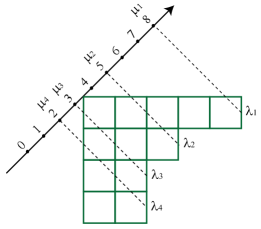
Figure 1: Graphical correspondence between the Young diagram of partition ${\boldsymbol{\lambda}}=(5,3,2,2)$ and the parts of strict partition ${\boldsymbol{\mu}}=(8,5,3,2)$ for $M=8$, $N=4$.

Let us consider a partition ${\boldsymbol{\lambda}}_{N-k}$ of the length $l({\boldsymbol{\lambda}}_{N-k})=N-k$, where $k\leq N$, $N,k\in\bar{\mathbb{N}}$. Proceeding with ${\boldsymbol{\lambda}}_{N-k}$, we shall use the notation $\widehat{{\boldsymbol{\lambda}}}\equiv\widehat{{\boldsymbol{\lambda}}}_{N}$ for a partition of the length $l\big{(}\widehat{{\boldsymbol{\lambda}}}\big{)}=N$, which can be viewed as ${\boldsymbol{\lambda}}_{N-k}$ “elongated” by $k$ zero’s as follows:

$$\widehat{{\boldsymbol{\lambda}}}\equiv(\lambda_{1},\lambda_{2},\dots,\lambda_{N-k},0,0,\dots,0)\equiv({\boldsymbol{\lambda}}_{N-k},0,0,\dots,0).$$ (2.4)

It is appropriate to introduce a strict partition $\widehat{{\boldsymbol{\mu}}}$, $l(\widehat{{\boldsymbol{\mu}}})=N$:

$$\widehat{{\boldsymbol{\mu}}}\equiv\widehat{{\boldsymbol{\lambda}}}+{{\boldsymbol{\delta}}}_{N}=({{\boldsymbol{\lambda}}}_{N-k}+{{\boldsymbol{\delta}}}_{N-k}+{\bf k}_{N-k},{{\boldsymbol{\delta}}}_{k})=({\boldsymbol{\mu}}_{N-k}+{\bf k}_{N-k},{{\boldsymbol{\delta}}}_{k}),$$ (2.5)

where ${{\boldsymbol{\delta}}}_{N}$, ${{\boldsymbol{\delta}}}_{N-k}$, and ${{\boldsymbol{\delta}}}_{k}$ are the staircase partitions (2.3) of the lengths $N$, $N-k$, and $k$, respectively, and ${\bf k}_{N-k}$ is a “constant” partition $(k,k,\dots,k)$ of the length $N-k$.

Let us introduce $k$-tuple ${\bf i}\equiv{\bf i}_{k}\equiv(i_{1},i_{2},\dots,i_{k})$ consisting of strictly increasing integers $1\leq i_{1}<i_{2}<\cdots<i_{k}\leq N$, $1\leq k\leq N$. It is appropriate to introduce a relative complement of ${{\bf i}}$ in $[N]$ as $(N-k)$-tuple ${\complement_{N}{\bf i}}$:

$${\complement_{N}{\bf i}}\equiv[N]\backslash{\bf i}=\big{(}1,2,\dots,\check{i}_{1},\dots,\check{i}_{2},\dots,\check{i}_{k},\dots,N\big{)},$$ (2.6)

where $\check{i}_{l}$ implies that the sequence $1,2,\dots,N$ is missing the element ${i}_{l}$.

Let $N$-tuple of complex numbers ${\bf x}_{N}$ be given. Fixing $k$-tuple ${\bf i}$ and its complement ${\complement_{N}{\bf i}}$ (2.6), we introduce $k$-tuple ${\bf x}_{{\bf i}}$ and $(N-k)$-tuple ${\mathbf{x}_{{}_{\complement_{N}{\bf i}}}}$:

$$\mathbf{x}_{{\bf i}}\equiv(x_{i_{1}},x_{i_{2}},\dots,x_{i_{k}}),$$ (2.7)

$${\mathbf{x}_{{}_{\complement_{N}{\bf i}}}}\equiv(x_{1},x_{2},\dots,\check{x}_{i_{1}},\dots,\check{x}_{i_{2}},\dots,\check{x}_{i_{k}},\dots,x_{N})\equiv\overline{\mathbf{x}_{\bf i}},$$ (2.8)

where $\check{x}_{i_{l}}$ implies that ${x}_{i_{l}}$ is dropped out of $N$-tuple $\mathbf{x}_{N}$. The equivalent notation $\overline{\mathbf{x}_{\bf i}}\equiv\mathbf{x}_{N}\backslash{\bf x}_{{\bf i}}$ (2.8) is to express that ${\mathbf{x}_{{}_{\complement_{N}{\bf i}}}}$ is also viewed as a relative complement of $k$-tuple ${\bf x}_{{\bf i}}$ (2.7) in $\mathbf{x}_{N}$. Besides, we shall use the following notation:

$$[N\backslash k]\equiv[N]\backslash[k].$$ (2.9)

We shall also consider $\mathbf{x}_{[k]}$ and $\mathbf{x}_{[N\backslash k]}$, as notations at ${\bf i}\equiv[k]$ for particular cases of ${\bf x}_{\bf i}$ and ${\bf x}_{[N]\backslash{\bf i}}$, respectively:

$$\mathbf{x}_{[k]}\equiv(x_{1},x_{2},\dots,x_{k}),\qquad{\mathbf{x}_{[N\backslash k]}}\equiv(x_{k+1},x_{k+2},\dots,x_{N})$$ (2.10)

(it turns out that $\mathbf{x}_{[k]}$ and $\mathbf{x}_{k}$ denote the same).

Let us introduce a plane partition of shape ${\boldsymbol{\lambda}}$ as a map $\boldsymbol{\pi}$: $(i,j)\rightarrow\pi_{ij}$, $(i,j)\in{\mathbb{N}}^{2}$, from the Young diagram of partition ${\boldsymbol{\lambda}}$ to $\bar{\mathbb{N}}$ such that $\pi_{ij}$ is a non-increasing function of $i$ and $j$. The entries $\pi_{ij}$ are called parts of the plane partition, and $|\boldsymbol{\pi}|=\sum_{i,j}\pi_{ij}$ is its volume.

Three-dimensional Young diagram is a stack of unit cubes such that $\pi_{ij}$ is the height of the column with coordinates $(i,j)$. A box ${\cal B}(L,N,K)$ of size $L\times N\times K$ is a subset of three-dimensional integer lattice:

$${\cal B}(L,N,K)\equiv\bigl{\{}(l,n,k)\in{\bar{\mathbb{N}}}^{3}\bigl{|}0\leq l\leq L,\,0\leq n\leq N,\,0\leq k\leq K\bigr{\}}.$$

It is said that a plane partition $\boldsymbol{\pi}$ is contained in ${\cal B}(L,N,K)$ if $i\leq L$, $j\leq N$, and $\pi_{ij}\leq K$ for all cubes of the Young diagram.

The generating function $Z_{q}(L,N,K)$ of plane partitions $\boldsymbol{\pi}$ contained in ${\cal B}(L,N,K)$ is of the form [32]:

$$Z_{q}(L,N,K)=\prod\limits_{j=1}^{L}\prod\limits_{k=1}^{N}\prod\limits_{i=1}^{K}\frac{1-q^{i+j+k-1}}{1-q^{i+j+k-2}}=\prod\limits_{j=1}^{L}\prod\limits_{k=1}^{N}\frac{1-q^{K+j+k-1}}{1-q^{j+k-1}}.$$ (2.11)

Right-hand side of (2.11) gives at $q\to 1$ the number $A(L,N,K)$ of plane partitions in the box ${\cal B}(L,N,K)$ (MacMahon’s formula):

$$A(L,N,K)=\prod\limits_{j=1}^{L}\prod\limits_{k=1}^{N}\prod\limits_{i=1}^{K}\frac{i+j+k-1}{i+j+k-2}=\prod\limits_{j=1}^{L}\prod\limits_{k=1}^{N}\frac{K+j+k-1}{j+k-1}.$$ (2.12)

2.2 The Cauchy–Binet type identities

The Schur functions $S_{{\boldsymbol{\lambda}}}({\textbf{x}}_{N})$ forming a basis for the ring of symmetric polynomials of $N$ variables are given by the relation (see [20, 32] for details):

$$S_{{\boldsymbol{\lambda}}}({\textbf{x}}_{N})\equiv S_{{\boldsymbol{\lambda}}}(x_{1},x_{2},\dots,x_{N})\equiv\frac{\det\big{(}x_{j}^{\lambda_{k}+N-k}\big{)}_{1\leq j,k\leq N}}{\mathcal{V}({\textbf{x}}_{N})},$$ (2.13)

where ${\boldsymbol{\lambda}}$ is a partition, and $\mathcal{V}({\textbf{x}}_{N})$ is the Vandermonde determinant,

$$\mathcal{V}({\textbf{x}}_{N})\equiv\det\big{(}x_{j}^{N-k}\big{)}_{1\leq j,k\leq N}=\prod_{1\leq m<l\leq N}(x_{l}-x_{m}).$$ (2.14)

Bearing in mind the notations (2.6), (2.7), (2.8), (2.9), (2.10), we turn to

Proposition 2.1.

Let us choose $k$-tuple ${\bf i}=(i_{1},i_{2},\dots,i_{k})$ and a partition ${{\boldsymbol{\lambda}}}_{N-k}$. The relation for the Schur function $S_{{\boldsymbol{\Lambda}}}(\mathbf{x}_{N})$ labelled by partition ${\boldsymbol{\Lambda}}$, $l({\boldsymbol{\Lambda}})=N$, holds true,

$$\lim_{{\bf x}_{{\bf i}}\rightarrow 0}S_{{\boldsymbol{\Lambda}}}(\mathbf{x}_{N})\equiv\lim_{x_{i_{1}}\rightarrow 0}\lim_{x_{i_{2}}\rightarrow 0}\cdots\lim_{x_{i_{k}}\rightarrow 0}S_{{\boldsymbol{\Lambda}}}(\mathbf{x}_{N})=S_{{{\boldsymbol{\lambda}}}_{N-k}}({\overline{\mathbf{x}_{\bf i}}}),$$ (2.15)

provided that $\boldsymbol{\Lambda}$ is of the form $\widehat{{\boldsymbol{\lambda}}}$ (2.4), and $\overline{\mathbf{x}_{\bf i}}$ (2.8) is used in (2.15).

The representation (2.13) enables to prove (2.15) provided that expansion of the determinants by minors is used iteratively when sending the elements of ${\bf x}_{{\bf i}}$ to zero.

The present section is concerned with the Cauchy–Binet type determinantal identity for the Schur functions [4]:

$$\mathcal{P}_{{\cal L}/n}(\textbf{x}_{N},\textbf{y}_{N})\equiv\sum_{{\boldsymbol{\lambda}}\subseteq{\{({\cal L}/n)^{N}\}}}S_{{\boldsymbol{\lambda}}}(\textbf{x}_{N})S_{{\boldsymbol{\lambda}}}(\textbf{y}_{N})=\Bigg{(}\prod_{l=1}^{N}x_{l}^{n}y_{l}^{n}\Bigg{)}\frac{\det T(\textbf{x}_{N},\textbf{y}_{N})}{\mathcal{V}(\textbf{x}_{N})\mathcal{V}(\textbf{y}_{N})},$$ (2.16)

where the summation goes over all partitions ${\boldsymbol{\lambda}}$ of length $N$ with the parts satisfying (2.2). The matrix $T(\textbf{x}_{N},\textbf{y}_{N})$ $\equiv$ $(T_{ij}(\textbf{x}_{N},\textbf{y}_{N}))_{1\leq i,j\leq N}$ in (2.16) is given by the entries

$$T_{ij}(\textbf{x}_{N},\textbf{y}_{N})\equiv T_{ij}=\frac{1-(x_{i}y_{j})^{N+{\cal L}-n}}{1-x_{i}y_{j}}.$$ (2.17)

If we put, for shortness, $\mathcal{P}_{{\cal L}/0}(\textbf{x}_{N},\textbf{y}_{N})\equiv\mathcal{P}_{{\cal L}}(\textbf{x}_{N},\textbf{y}_{N})$, equation (2.16) is re-expressed as

$$\mathcal{P}_{{\cal L}/n}(\textbf{x}_{N},\textbf{y}_{N})=\mathcal{P}_{{\cal L}-n}(\textbf{x}_{N},\textbf{y}_{N})\prod_{l=1}^{N}(x_{l}y_{l})^{n}.$$ (2.18)

Proposition 2.1 allows us to go from the sum $\mathcal{P}_{\cal L}(\textbf{x}_{N},\textbf{y}_{N})$ (2.16) to the sum $\mathcal{P}_{\cal L}(\overline{\mathbf{x}_{\bf i}},\textbf{y}_{N})$ one of the arguments of which is $(N-k)$-tuple $\overline{\mathbf{x}_{\bf i}}\equiv\textbf{x}_{[N]\backslash{\bf i}}$ (2.8):

$$\mathcal{P}_{\cal L}(\overline{\mathbf{x}_{\bf i}},\textbf{y}_{N})\equiv\sum\limits_{{\boldsymbol{\lambda}}\subseteq\{{\cal L}^{N-k}\}}S_{{\boldsymbol{\lambda}}}(\overline{\mathbf{x}_{\bf i}})S_{\widehat{\boldsymbol{\lambda}}}({\textbf{y}}_{N}),$$ (2.19)

where $k$-tuple ${\bf i}$ is fixed, summation is over ${\boldsymbol{\lambda}}$ of length $N-k$, and $\widehat{{\boldsymbol{\lambda}}}$ is given by (2.4). The determinantal identity for $\mathcal{P}_{\cal L}(\overline{\mathbf{x}_{\bf i}},\textbf{y}_{N})$, analogous to (2.16), is given by

Theorem 2.2.

The Cauchy–Binet type identity is valid for $\mathcal{P}_{\cal L}(\overline{\mathbf{x}_{\bf i}},\textbf{y}_{N})$ (2.19):

$$\mathcal{P}_{\cal L}(\overline{\mathbf{x}_{\bf i}},\textbf{y}_{N})=\frac{(-1)^{|{\bf i}|+kN-\frac{k}{2}(k-1)}}{\big{(}\prod_{l\in[N]\backslash{\bf i}}x_{l}\big{)}^{k}}\,\frac{\det{\overline{T}}(\overline{\mathbf{x}_{\bf i}},\textbf{y}_{N})}{{\mathcal{V}}(\overline{\mathbf{x}_{\bf i}}){\mathcal{V}}({\textbf{y}}_{N})},$$ (2.20)

where the entries of $N\times N$ matrix $\overline{T}(\overline{\mathbf{x}_{\bf i}},\textbf{y}_{N})\equiv(\overline{T}_{ij})_{1\leq i,j\leq N}$ are

$${\overline{T}}_{ij}=T^{\rm o}_{ij},\qquad i\in{\complement_{N}{\bf i}}=[N]\backslash{\bf i},\qquad 1\leq j\leq N,$$

$${\overline{T}}_{ij}=y_{j}^{k-l},\quad i\in\{i_{l}\}_{1\leq l\leq k},\qquad 1\leq j\leq N.$$ (2.21)

The entries $T^{\rm o}_{ij}$ are given by $T_{ij}$ (2.17) taken at $n=0$.

Proof.

The overall summation in left-hand side of equation (2.16) taken at $n=0$ splits into two parts: the sum over $\widehat{\boldsymbol{\lambda}}$ (2.4) (where ${\cal L}\geq\lambda_{1}\geq\lambda_{2}\geq\dots\geq\lambda_{N-k}\geq 0$) and the remaining sum. We apply $\lim_{{\bf x}_{{\bf i}}\rightarrow 0}$ (2.15) in both sides of (2.16). The relation $\mathcal{P}_{\cal L}(\overline{\mathbf{x}_{\bf i}},\textbf{y}_{N})=\lim_{{\bf x}_{{\bf i}}\rightarrow 0}\mathcal{P}_{\cal L}(\textbf{x}_{N},\textbf{y}_{N})$ holds since the only summation surviving in left-hand side of (2.16) is that over $\widehat{\boldsymbol{\lambda}}$, and we thus obtain (2.20) due to Proposition 2.1. ∎

Two limits of the identity (2.20) are of interest in what follows. In the first case, equation (2.15) is specified:

$$\lim_{\mathbf{x}_{[k]}\rightarrow 0}S_{\widehat{{\boldsymbol{\lambda}}}}(\mathbf{x}_{N})=S_{{{\boldsymbol{\lambda}}}_{N-k}}\big{(}\mathbf{x}_{[N\backslash k]}\big{)},$$ (2.22)

where the relations (2.10) are taken into account. In the second one, equation (2.15) reads:

$$\lim_{\mathbf{x}_{{\mathbf{N}_{k}}\backslash{{{\boldsymbol{\delta}}}_{k}}}\rightarrow 0}S_{\widehat{{\boldsymbol{\lambda}}}}(\mathbf{x}_{N})=S_{{{\boldsymbol{\lambda}}}_{N-k}}(\mathbf{x}_{N-k}),$$ (2.23)

where ${\mathbf{x}}_{\mathbf{N}_{k}\backslash{{{\boldsymbol{\delta}}}_{k}}}\equiv(x_{N-k+1},x_{N-k+2},\dots,x_{N-1},x_{N})$, and the relation

$$\mathbf{x}_{[N]\backslash({\mathbf{N}_{k}}\backslash{{{\boldsymbol{\delta}}}_{k}})}=\mathbf{x}_{N-k}$$ (2.24)

is accounted for.

Let us define a $q$-number $[n]$ ($n\in\bar{\mathbb{N}}$) and $q$-factorial $[n]!$ [28]:

$$[n]\equiv\frac{1-q^{n}}{1-q},\qquad[n]!\equiv[1][2]\cdots[n],\qquad[0]!\equiv 1.$$ (2.25)

This definition allows to define the q-binomial coefficient $\left[\begin{smallmatrix}N\\ r\end{smallmatrix}\right]$,

$$\begin{bmatrix}N\\ r\end{bmatrix}\equiv\frac{[N][N-1]\cdots[N-r+1]}{[r]!}=\frac{[N]!}{[r]![N-r]!},$$ (2.26)

as well as the $q$-binomial determinant [10]:

$$\begin{pmatrix}{\bf{a}}\\ {\bf{b}}\end{pmatrix}_{q}\equiv\begin{pmatrix}a_{1},&a_{2},&\cdots&a_{S}\\ b_{1},&b_{2},&\cdots&b_{S}\end{pmatrix}_{q}\equiv\det\begin{pmatrix}\begin{bmatrix}a_{j}\\ b_{i}\end{bmatrix}\end{pmatrix}_{1\leq i,j\leq S},$$ (2.27)

where ${\bf{a}}$ and ${\bf{b}}$ are ordered $S$-tuples: $0\leq a_{1}<a_{2}<\cdots<a_{S}$ and $0\leq b_{1}<b_{2}<\cdots<b_{S}$. In the limit $q\to 1$, the $q$-binomial determinant (2.27) is transformed to the binomial determinant since (2.26) becomes the binomial coefficient $\left(\begin{smallmatrix}N\\ r\end{smallmatrix}\right)$ [21].

The $q$-parametrization

$$\textbf{y}_{N}={\bf q}_{N}\equiv\big{(}q,q^{2},\dots,q^{N}\big{)},\qquad\textbf{x}_{N}={\bf q}_{N}/q=\big{(}1,q,\dots,q^{N-1}\big{)}$$ (2.28)

enables to represent the sum $\mathcal{P}_{\cal L}(\overline{\mathbf{x}_{\bf i}},\textbf{y}_{N})$ (2.19) in the form:

$$\mathcal{P}_{\cal L}\bigg{(}\frac{\overline{\mathbf{q}_{\bf i}}}{q},{\bf q}_{N}\bigg{)}=\sum\limits_{{\boldsymbol{\lambda}}\subseteq\{{\cal L}^{N-k}\}}S_{\widehat{\boldsymbol{\lambda}}}({\textbf{q}}_{N})S_{{\boldsymbol{\lambda}}}\bigg{(}\frac{\overline{\mathbf{q}_{\bf i}}}{q}\bigg{)},$$ (2.29)

where

$$\overline{\mathbf{q}_{\bf i}}\equiv\big{(}q,q^{2},\dots,\underset{\smile}{{{q}^{i_{{}_{1}}}}},\dots,\underset{\smile}{{{q}^{i_{{}_{2}}}}},\dots,\underset{\smile}{{{q}^{i_{{}_{k}}}}},\dots,q^{N}\big{)},$$

and the underscored terms are missed. One arrives to the following

Claim 2.3.

The Cauchy–Binet type identity (2.20) under the $q$-parametrization (2.28) is valid for $\mathcal{P}_{\cal L}\big{(}\frac{\overline{\mathbf{q}_{\bf i}}}{q},{\bf q}_{N}\big{)}$ (2.29):

$$\mathcal{P}_{\cal L}\bigg{(}\frac{\overline{\mathbf{q}_{\bf i}}}{q},{\bf q}_{N}\bigg{)}=\frac{(-1)^{|{\bf i}|+kN-\frac{k}{2}(k-1)}}{q^{k(k-|{\bf i}|)+\frac{kN}{2}(N-1)}}\,\frac{\det\overline{\sf T}\bigl{(}\frac{\overline{\mathbf{q}_{\bf i}}}{q},{\bf q}_{N}\bigr{)}}{{\mathcal{V}}\bigl{(}\frac{\overline{\mathbf{q}_{\bf i}}}{q}\bigr{)}{\mathcal{V}}({\bf q}_{N})},$$ (2.30)

where the matrix $\overline{\sf T}\bigl{(}\frac{\overline{\mathbf{q}_{\bf i}}}{q},{\bf q}_{N}\bigr{)}$ consists of $q$-parameterized entries ${\overline{\sf T}}_{ij}$ (2.21):

$$\overline{\sf T}_{ij}=\frac{[({\cal L}+N)(j+i-1)]}{[j+i-1]},\qquad i\in[N]\backslash{\bf i},\qquad 1\leq j\leq N,$$

$$\overline{\sf T}_{ij}=q^{j(k-l)},\qquad i\in\{i_{l}\}_{1\leq l\leq k},\qquad 1\leq j\leq N,$$ (2.31)

and $q$-numbers (2.25) are used.

The parametrisation of the identity (2.30) is concretized as ${\overline{\mathbf{q}_{\bf i}}}={{\mathbf{q}_{[N\backslash k]}}}$ for ${\bf i}_{k}=[k]$ in the case (2.22), or ${\overline{\mathbf{q}_{\bf i}}}={{\mathbf{q}_{N-k}}}$ for ${\bf i}_{k}={\bf N}_{k}\backslash{{\boldsymbol{\delta}}}_{k}$ in the case (2.23). The Schur functions $S_{{\boldsymbol{\lambda}}_{N-k}}\bigl{(}\frac{\overline{\mathbf{q}_{\bf i}}}{q}\bigr{)}$ in these cases are related to each other (see (2.24) for the second case):

$$S_{{\boldsymbol{\lambda}}_{N-k}}\bigg{(}\frac{{\bf q}_{[N\backslash k]}}{q}\bigg{)} \equiv S_{{\boldsymbol{\lambda}}_{N-k}}(q^{k},q^{k+1},\dots,q^{N-1})=q^{k|{{\boldsymbol{\lambda}}}|}S_{{\boldsymbol{\lambda}}_{N-k}}\bigg{(}\frac{{\bf q}_{N-k}}{q}\bigg{)}$$

$$=q^{k|{{\boldsymbol{\lambda}}}|}S_{{\boldsymbol{\lambda}}_{N-k}}\bigg{(}\frac{{\bf q}_{[N]\backslash({\mathbf{N}_{k}}\backslash{{{\boldsymbol{\delta}}}_{k}})}}{q}\bigg{)}.$$ (2.32)

The Claim 2.3 is to stress that equation (2.30) generalizes the relationship between ${{\mathcal{P}}}_{\cal L}\bigl{(}\frac{{\bf q}_{N-k}}{q},{\bf q}_{N}\bigr{)}$ and $\det\overline{\sf T}\bigl{(}\frac{{\bf q}_{N-k}}{q},{\bf q}_{N}\bigr{)}$ found in [4] and given by

Theorem 2.4.

The sum ${{\mathcal{P}}}_{\cal L}\bigl{(}\frac{{\bf q}_{N-k}}{q},{\bf q}_{N}\bigr{)}$ expressed by (2.29) at ${\bf i}_{k}={\bf N}_{k}\backslash{{\boldsymbol{\delta}}}_{k}$ satisfies the following identities:

$${\mathcal{P}}_{\cal L}\bigg{(}\frac{{\bf q}_{N-k}}{q},{\bf q}_{N}\bigg{)} =q^{-\frac{k}{2}(N-k-1)(N-k)}\frac{{\det}\overline{\sf T}\bigl{(}\frac{{\bf q}_{N-k}}{q},{\bf q}_{N}\bigr{)}}{{\mathcal{V}}({\bf q}_{N}){\mathcal{V}}({\bf q}_{N-k}/q)}$$ (2.33)

$$=q^{-\frac{N}{2}({\cal L}-1){\cal L}}\begin{pmatrix}2N-k,&2N-k+1,&\cdots&2N-k+{\cal L}-1\\ N-k,&N-k+1,&\cdots&N-k+{\cal L}-1\end{pmatrix}_{q}$$ (2.34)

$$=\prod_{l=1}^{{\cal L}}\prod_{j=1}^{N-k}\frac{[j+l+N-1]}{[j+l-1]}=Z_{q}(N-k,N,{\cal L}).$$ (2.35)

Proof.

Connection between the Schur functions and the elementary symmetric functions [32] allows one to derive (2.34), [4]. Evaluation of the $q$-binomial determinant (2.34) results in the double product representation (2.35), which is the generating function of plane partitions in ${\cal B}(N-k,N,{\cal L})$ since $Z_{q}(N-k,{\cal L},N)$ is equal to $Z_{q}(N-k,N,{\cal L})$), [3]. ∎

The $q$-version of (2.16) arises from (2.34), (2.35) at $k=0$ due to (2.18):

$${{\mathcal{P}}}_{{\cal L}/n}({\bf q}_{N}/q,{\bf q}_{N}) =q^{nN^{2}}q^{\frac{N({\cal L}-n)}{2}(1-{\cal L}+n)}\det\left(\displaystyle{\begin{bmatrix}2N+i-1\\ N+j-1\end{bmatrix}}\right)_{1\leq i,j\leq{\cal L}-n}$$ (2.36)

$$=q^{nN^{2}}Z_{q}(N,N,{\cal L}-n),$$ (2.37)

where $Z_{q}(N,N,{\cal L}-n)$ is the generating function (2.11) of plane partitions in the box ${\cal B}(N,N,\allowbreak{\cal L}-n)$. The number of plane partitions $A(N,N,{\cal L}-n)$ is obtained as (2.12):

$$A(N,N,{\cal L}-n)=\prod_{l=1}^{N}\prod_{j=1}^{N}\frac{{\cal L}-n+j+l-1}{j+l-1}.$$ (2.38)

3 The Schur functions and watermelons

A combinatorial interpretation of the Cauchy–Binet type identities (2.16), (2.20), and (2.30), is provided in the present section in terms of the watermelon configurations of self-avoiding lattice paths.

3.1 The Schur functions and stars

3.1.1 Stars without deviation

Let a set $\{\sf{T}\}$ of semi-standard Young tableaux ${\sf{T}}$ of shape ${{\boldsymbol{\lambda}}}={{\boldsymbol{\lambda}}}_{N}$, [20], with the entries taken from the set $[N]$ is given. Each semi-standard tableau of shape ${{\boldsymbol{\lambda}}}$ may be represented as a nest of self-avoiding lattice paths with prescribed starting and ending points. Consider a grid of vertical and horizontal dashed lines enumerated as in Figure 2.

Figure 2: The star $\cal{C}$ representing the semistandard tableau of shape ${\boldsymbol{\lambda}}=(6,3,3,1)$.

The star [23, 29] is the nest of paths introduced by means of

Definition 3.1.

The star $\cal{C}$, corresponding to the semi-standard Young tableau of shape ${{\boldsymbol{\lambda}}}$, is a nest of $N$ self-avoiding lattice paths that connect (Figure 2) the equidistantly arranged starting points $C_{i}=(i,N-i)$ with the non-equidistant ending points $(N,\mu_{i})$, where the parts of a strict partiton ${\boldsymbol{\mu}}$ respect (2.1) at $n=0$, while the parts $\lambda_{i}=\mu_{i}-N+i$, $1\leq i\leq N$, respect (2.2) with ${\cal L}={\cal M}$, where ${\cal M}\equiv M-N+1$.

The $i^{\rm th}$ row of the tableau ${\sf{T}}$ is encoded by $i^{\rm th}$ path of $\cal{C}$ making $\lambda_{i}$ steps upward. The number of steps along the sites with abscissa $x_{j}$ is equal to the number of occurrences of $j$ in the $i^{\rm th}$ row of ${\sf{T}}$. We put ${\bf x}_{N}\equiv(x_{1},x_{2},\dots,x_{N})$ so that the Schur function equivalent to (2.13) is defined [20]:

$$S_{{\boldsymbol{\lambda}}}({\bf x}_{N})=\sum_{\{{\sf{T}}\}}\prod_{i,j}x_{{}_{{\sf{T}}_{ij}}}=\sum_{\{\cal{C}\}}\prod_{j=1}^{N}x_{j}^{c_{j}},$$ (3.1)

where the middle sum is over all tableaux ${\sf{T}}$ of shape ${{\boldsymbol{\lambda}}}$, and the product of $x_{{}_{{\sf{T}}_{ij}}}$ is over all entries of ${\sf{T}}$. Summation in right-hand side of (3.1) is over all admissible $\cal{C}$, and $c_{j}$ is the number of steps upward along the vertical line with abscissa $x_{j}$. It follows from (3.1) that $S_{{\boldsymbol{\lambda}}}({\bf 1}_{N})$ is the total number of the nests of paths [32]:

$$S_{{\boldsymbol{\lambda}}}({\bf 1}_{N})=\sum_{\{\cal{C}\}}1=\prod_{1\leq j<k\leq N}\frac{\lambda_{j}-j-\lambda_{k}+k}{k-j}.$$ (3.2)

Each lattice path belonging to $\cal C$ can be enclosed by a rectangle so that the path’s starting point coincides with the lower left vertex. The size of rectangle for $i^{\rm th}$ path is $\lambda_{i}\times(N-i)$, $1\leq i\leq N$. The volume of the path is the number of cells below the path within the corresponding rectangle. The volume $|{\cal C}|$ of the star $\cal C$ is equal to the sum of the volumes of the paths:

$$|{\cal C}|=\sum_{j=1}^{N}(N-j)c_{j}=N|{{\boldsymbol{\lambda}}}|-\sum_{j=1}^{N}jc_{j},$$

since $\sum_{j=1}^{N}c_{j}=|{\boldsymbol{\lambda}}|$ is the weight of ${{\boldsymbol{\lambda}}}$. The partition function of the stars $\cal C$ defined as ${\cal Z}_{\{\cal{C}\}}=\sum_{\{\cal{C}\}}q^{\mid{\cal C}\mid}$ is expressed through the Schur function (3.1) at ${\bf x}_{N}={\bf q}_{N}/q$:

$${\cal Z}_{\{\cal{C}\}}=\sum_{\{\cal{C}\}}q^{\mid{\cal C}\mid}=q^{N|{{\boldsymbol{\lambda}}}|}\sum_{\{\cal{C}\}}q^{-\sum_{j=1}^{N}jc_{j}}=q^{N|{{\boldsymbol{\lambda}}}|}S_{{\boldsymbol{\lambda}}}\bigg{(}\frac{1}{\textbf{q}_{N}}\bigg{)}=S_{{\boldsymbol{\lambda}}}\bigg{(}\frac{\textbf{q}_{N}}{q}\bigg{)}=q^{-|{{\boldsymbol{\lambda}}}|}S_{{\boldsymbol{\lambda}}}(\textbf{q}_{N}).$$ (3.3)

Equation (3.3) expresses that $\{\cal{C}\}$ is determined by a choice of ${\boldsymbol{\lambda}}$.

Taking into account (3.3), it is appropriate to introduce the extended volume $|{\cal C}|_{\rm w}$ (see Figure 2):

$$|{\cal C}|_{\rm w}\equiv|{\cal C}|+|{\boldsymbol{\lambda}}|=(N+1)|{{\boldsymbol{\lambda}}}|-\sum_{j=1}^{N}jc_{j}.$$ (3.4)

Although the star in Figure 2 is presented for $N=4$, one extra column of cells is added between the lines with abscissae $N$ and $N+1$. To admit a single rightward step for each path in the nest is the same as to add $|{\boldsymbol{\lambda}}|$ to $|{\cal C}|$ thus obtaining $|{\cal C}|_{\rm w}$. The definition (3.4) enables the following identity:

$$\sum_{\{\cal{C}\}}q^{|{\cal C}|_{\rm w}}=q^{|{{\boldsymbol{\lambda}}}|}S_{{\boldsymbol{\lambda}}}\Bigl{(}\frac{\textbf{q}_{N}}{q}\Bigr{)}=S_{{\boldsymbol{\lambda}}}(\textbf{q}_{N}).$$ (3.5)

Let us introduce the partition ${\mathbb{M}}\equiv({\mathcal{M}},{\cal M},\dots,{\mathcal{M}})$ of the length $l({\mathbb{M}})=N$, where ${\mathcal{M}}$ is given by Definition 3.1, and let us advance

Definition 3.2.

The conjugate star $\cal{B}$, corresponding to the semi-standard skew Young tableau of shape ${\mathbb{M}}\backslash{{\boldsymbol{\lambda}}}$, is a configuration of $N$ self-avoiding lattice paths (as depicted in Figure 3) that connect the non-equidistant points $(1,\mu_{\alpha})$, where $\mu_{\alpha}=\lambda_{\alpha}+N-{\alpha}$, $1\leq{\alpha}\leq N$, with the equidistantly arranged points $B_{\alpha}=({\alpha},M+1-{\alpha})$.

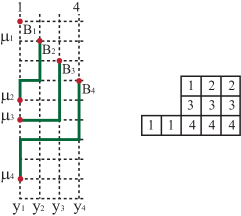
Figure 3: Conjugate star ${\cal B}$ and the corresponding skew tableau ${\sf{T_{{\mathbb{M}}\backslash{{\boldsymbol{\lambda}}}}}}$ of shape ${\mathbb{M}}\backslash{{\boldsymbol{\lambda}}}$.

Each path in the conjugate star ${\cal B}$ is enclosed by rectangle of the size $({\mathcal{M}}-\lambda_{\alpha})\times({\alpha}-1)$. The volume of path in ${\cal B}$ is the number of cells above the path inside the corresponding rectangle (see Figure 3). The volume of ${\cal B}$ is $|{\cal B}|=\sum_{{\alpha}=1}^{N}b_{\alpha}({\alpha}-1)$, where $b_{\alpha}$ is the number of steps along abscissa $y_{\alpha}$.

The $\alpha^{\rm th}$ path of $\cal{B}$ making ${\mathcal{M}}-\lambda_{\alpha}$ upward steps encodes the $\alpha^{\rm th}$ row of the skew tableau ${\sf{T_{{\mathbb{M}}\backslash{{\boldsymbol{\lambda}}}}}}$ of shape ${\mathbb{M}}\backslash{{\boldsymbol{\lambda}}}$. The number of steps along the sites with abscissa $y_{\beta}$ is equal to the number of occurrences of $\beta$ in $\alpha^{\rm th}$ row of ${\sf{T_{{\mathbb{M}}\backslash{{\boldsymbol{\lambda}}}}}}$ (Figure 3). Since ${\sf{T_{{\mathbb{M}}\backslash{{\boldsymbol{\lambda}}}}}}$ and ${\sf{T_{{{\boldsymbol{\lambda}}}}}}$ are in involution [45], the corresponding Schur functions are coinciding. Thus we put ${\bf y}\equiv(y_{1},y_{2},\dots,y_{N})$ and obtain

$$S_{{\mathbb{M}}\backslash{\boldsymbol{\lambda}}}({\bf y})=\displaystyle{\frac{\det\big{(}y_{\alpha}^{{\mathcal{M}}-\lambda_{N-{\beta}+1}+N-{\beta}}\big{)}_{1\leq{\alpha},{\beta}\leq N}}{\det(y_{\alpha}^{N-{\beta}})_{1\leq{\alpha},{\beta}\leq N}}}=\sum_{\{\cal{B}\}}\prod_{{\alpha}=1}^{N}y_{{\alpha}}^{b_{\alpha}}.$$ (3.6)

Proposition 3.3.

The following representation of the Schur function $S_{{\boldsymbol{\lambda}}}({\bf y})$ is valid:

$$S_{{\boldsymbol{\lambda}}}({\bf y})=\sum_{\{\cal{B}\}}\prod_{{\alpha}=1}^{N}y_{{\alpha}}^{{\mathcal{M}}-b_{\alpha}}.$$ (3.7)

Proof.

Equation (3.7) is valid since factorizing out $\prod_{{\alpha}=1}^{N}y_{\alpha}^{\mathcal{M}}$ from left-hand side of (3.6), after some transformation one obtains [42]:

$$S_{{\mathbb{M}}\backslash{\boldsymbol{\lambda}}}({\bf y})=S_{{\boldsymbol{\lambda}}}\bigg{(}\frac{1}{\bf y}\bigg{)}\prod_{{\alpha}=1}^{N}y_{{\alpha}}^{{\mathcal{M}}}.$$ ∎

The representation (3.7) connects the Schur function labelled by ${{\boldsymbol{\lambda}}}$ to the parameters of the conjugate stars ${\cal B}$.

Let us introduce two volumes of the conjugate star ${\cal B}$, namely, a dual volume $|{\cal B}|_{\rm d}$,

$$|{\cal B}|_{\rm d}=\sum_{{\alpha}=1}^{N}({\mathcal{M}}-\lambda_{\alpha}-b_{\alpha})({\alpha}-1),$$ (3.8)

and a dual extended volume $|{\cal B}|_{\rm w}$,

$$|{\cal B}|_{\rm w}\equiv|{\cal B}|_{\rm d}+n({{\boldsymbol{\lambda}}})=\sum_{{\alpha}=1}^{N}({\mathcal{M}}-b_{\alpha})({\alpha}-1),\qquad n({{\boldsymbol{\lambda}}})\equiv\sum_{{\alpha}=1}^{N}\lambda_{\alpha}({\alpha}-1).$$ (3.9)

While $|{\cal B}|_{\rm d}$ (3.8) “counts” the cells below the paths in ${\cal B}$, the definition (3.9) gives $|{\cal B}|_{\rm w}$ as “shifted” $|{\cal B}|_{\rm d}$.

The partition function of the star $\cal B$, Figure 3, is obtained from (3.7) under the parametrization ${\bf y}={\bf q}_{N}/q$:

$$S_{{\boldsymbol{\lambda}}}\bigg{(}\frac{\textbf{q}_{N}}{q}\bigg{)}=\sum_{\{{\cal B}\}}q^{\sum_{j=1}^{N}(j-1)({\mathcal{M}}-b_{j})}=\sum_{\{{\cal B}\}}q^{|{\cal B}|_{\rm w}},$$ (3.10)

where equation (3.9) is used, and summation is over all stars $\cal{B}$. It is seen from (3.6) that $|{\cal B}|$ is connected with the Schur function that corresponds to the skew partition ${\mathbb{M}}\backslash{\boldsymbol{\lambda}}$. In the limit $q\rightarrow 1$, the Schur functions (3.5) and (3.10) are equal to the number of stars either $\cal{B}$ or $\cal{C}$: $S_{{\boldsymbol{\lambda}}}({\bf{1}}_{N})=\sum_{\{\cal{B}\}}1=\sum_{\{\cal{C}\}}1$.

3.1.2 Stars with deviation

Regarding the star ${\cal C}$ above, let us introduce the star ${\cal C}_{k}$ with deviation $k$ by means of

Definition 3.4.

The star ${\cal C}_{k}$ with deviation $k$ is the nest of lattice paths like the nest ${\cal C}$ without upward steps along the lines with abscissae $x_{1},x_{2},\dots,x_{k}$. The star ${\cal C}_{k}$ is characterized by such semi-standard Young tableau of shape ${{\boldsymbol{\lambda}}}_{N-k}$ that the number inside the upper left corner cell is greater than $k$ (see Figure 4).

The Schur function associated with the star ${\cal C}_{k}$ is represented like (3.1):

$$S_{{{\boldsymbol{\lambda}}}}(\mathbf{x}_{[N\backslash k]})=\sum_{\{{\cal C}_{k}\}}\prod_{j=k+1}^{N}x_{j}^{c_{j}},$$ (3.11)

where ${{\boldsymbol{\lambda}}}\equiv{{\boldsymbol{\lambda}}}_{N-k}$ and $\mathbf{x}_{[N\backslash k]}$ (2.10) is used. The representation (3.11) is in agreement with the representation (3.1) subjected to the limit (2.22) provided that $c_{1}=c_{2}=\dots=c_{k}=0$.

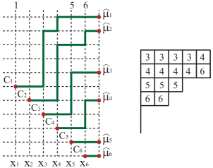
Figure 4: The star ${\cal{C}}_{k}$ with deviation $k=2$ given by ${\widehat{\boldsymbol{\mu}}}=(10,9,6,4,1,0)$ represents the semi-standard tableau of shape ${\widehat{\boldsymbol{\lambda}}}=(5,5,3,2,0,0)$.

By analogy with (3.4), we introduce the extended volume $|{\cal C}_{k}|_{\rm w}$ of the star ${\cal C}_{k}$:

$$|{\cal C}_{k}|_{\rm w}\equiv(N+1)|{{\boldsymbol{\lambda}}}_{N-k}|-\sum_{j=k+1}^{N}jc_{j},$$ (3.12)

where $\sum_{j=k+1}^{N}c_{j}=|{{\boldsymbol{\lambda}}}_{N-k}|$ since $c_{1}=c_{2}=\dots=c_{k}=0$, and the corresponding partition function is expressed:

$${\cal Z}_{\{{\cal C}_{k}\}}=\sum_{\{{\cal C}_{k}\}}q^{\mid{\cal C}_{k}\mid_{\rm w}}=q^{(N+1)|{{\boldsymbol{\lambda}}}_{N-k}|}S_{{{\boldsymbol{\lambda}}}_{N-k}}\bigg{(}\frac{1}{\textbf{q}_{[N\backslash k]}}\bigg{)}=S_{{{\boldsymbol{\lambda}}}_{N-k}}({\textbf{q}_{N-k}}).$$ (3.13)

The modification of the volume in the form

$$|{\cal C}_{k}|_{\overline{\rm w}}\equiv(N+k+1)|{{\boldsymbol{\lambda}}}_{N-k}|-\sum_{j=k+1}^{N}jc_{j}$$ (3.14)

leads to the partition function

$${\cal Z}_{\{{\cal C}_{k}\}}=\sum_{\{{\cal C}_{k}\}}q^{\mid{\cal C}_{k}\mid_{\overline{\rm w}}}=q^{k|{{\boldsymbol{\lambda}}}_{N-k}|}S_{{{\boldsymbol{\lambda}}}_{N-k}}({\textbf{q}_{N-k}})=S_{{{\boldsymbol{\lambda}}}_{N-k}}\big{(}\textbf{q}_{[N\backslash k]}\big{)}.$$ (3.15)

The volumes (3.12) and (3.14) ensure (2.32). Both (3.13) and (3.15) are reduced at $k=0$ to (3.5).

The conjugated star ${\cal B}_{k}$ with deviation $k$ is introduced by

Definition 3.5.

The star ${\cal B}_{k}$ is the nest of lattice paths like ${\cal B}$ supplied with the requirement that the number of upward steps along a vertical line with abscissa $y_{\alpha}$ for $N-k+1\leq\alpha\leq N$ is equal to ${\mathcal{M}}$ (see Figure 5).

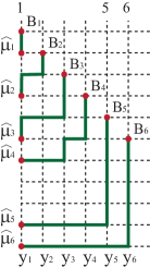
Figure 5: The star representing skew tableau ${\mathbb{M}}\backslash{\widehat{{\boldsymbol{\lambda}}}}$.

The limit (2.23) results in the Schur function corresponding to a skew tableau ${\mathbb{M}}\backslash{\widehat{{\boldsymbol{\lambda}}}}$, where ${\widehat{{\boldsymbol{\lambda}}}}$ is defined by (2.4). It is suggestive, regarding (3.7), to put

$$S_{{{\boldsymbol{\lambda}}}_{N-k}}({\bf y}_{N-k})=\sum_{\{{\cal B}_{k}\}}\prod\limits_{\alpha=1}^{N-k}y_{\alpha}^{{\mathcal{M}}-b_{\alpha}}.$$ (3.16)

Equation (3.16) is expressed under the parametrization ${\bf y}={\bf q}_{N}/q$:

$$S_{{{\boldsymbol{\lambda}}}_{N-k}}\bigg{(}\frac{{\bf q}_{N-k}}{q}\bigg{)}=\sum_{\{{\cal B}_{k}\}}q^{\mid{\cal B}_{k}\mid_{\rm w}},\qquad|{\cal B}_{k}|_{\rm w}\equiv\sum_{{\alpha}=1}^{N-k}({\mathcal{M}}-b_{\alpha})({\alpha}-1).$$

3.2 Watermelons and their generating functions

3.2.1 Watermelons without deviation

The watermelon configuration (see Figure 6($a$)) is represented by the nest of self-avoiding lattice paths with equidistantly arranged starting $C_{l}$ and ending $B_{l}$ points ($1\leq l\leq N$). Only upward and rightward steps are allowed, and the nest is characterized by the paths with the total number of upward steps ${\mathcal{M}}$ and the total number of rightward steps $N$. The $l^{\rm th}$ path in watermelon is contained within the rectangle such that $C_{l}$ and $B_{l}$ are its lower left and upper right vertices, respectively ($1\leq l\leq N$).

The nest of paths corresponding to watermelon results from

Construction 3.6.

Watermelon is the nest of paths obtained by “gluing” the stars ${\cal C}$ and ${\cal B}$ along the dissection line determined by the partition ${\boldsymbol{\mu}}$ with parts respecting (2.1) so that the points $(N+1,\mu_{i})$ (see Figure 2) and the points $(1,\mu_{i})$ (see Figure 3) are identified (Figure 6).

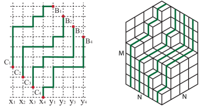
Figure 6: Watermelon configuration of self-avoiding paths ($a$) and related boxed plane partition with gradient lines ($b$).

The representations of the Schur functions (3.1) and (3.7) allow us to conclude that $\mathcal{P}_{{\cal L}/n}(\textbf{x}_{N},\textbf{y}_{N})$ (2.16) is related with summation over the nests of paths constituting the watermelon configurations, i.e.,

$$\mathcal{P}_{{\mathcal{M}}/n}(\textbf{x}_{N},\textbf{y}_{N})=\sum_{{\boldsymbol{\lambda}}\subseteq{\{({\mathcal{M}}/n)^{N}\}}}\Bigg{(}\sum_{\{\cal{C}\}}\prod_{j=1}^{N}x_{j}^{c_{j}}\Bigg{)}\Biggl{(}\sum_{\{\cal{B}\}}\prod_{{\alpha}=1}^{N}y_{{\alpha}}^{{\mathcal{M}}-b_{\alpha}}\Biggr{)},$$ (3.17)

may be considered as the generating function of the watermelon configurations, which are in a bijective correspondence with boxed plane partitions [23, 29].

Let us define the volume of the path as the number of cells below the path within the corresponding rectangle, and the volume of watermelon as the volume of all paths constituting the watermelon (see Figure 6).

If so, the numbers of nests of the lattice paths constituting the watermelons are encoded by the generating function of watermelons given by

Definition 3.7.

Let ${\bf w}_{N,{\mathcal{M}}/n}$ be a nest of $N$ paths constituting the watermelon. Each path in the nest consists of $N$ steps along the abscissa axis. The subscript ${\mathcal{M}}/n$ implies that $\mu_{N}\geq n$ and the number of steps along the ordinate axis is ${\mathcal{M}}$. The generating function $W_{q}(N,{\mathcal{M}}/n)$ of watermelons is defined as the polynomial

$$W_{q}(N,{\mathcal{M}}/n)\equiv\sum_{\{{\bf w}_{N,{\mathcal{M}}/n}\}}q^{|{\bf w}_{N,{\mathcal{M}}/n}|},$$ (3.18)

where summation is over all nests ${{\bf w}_{N,{\mathcal{M}}/n}}$, and $|{{\bf w}_{N,{\mathcal{M}}/n}}|$ is the volume of the nest:

$$|{{\bf w}_{N,{\mathcal{M}}/n}}|\equiv\sum_{j=1}^{2N}(2N-j)m_{j}-\frac{{\mathcal{M}}N}{2}(N-1)+\frac{nN}{2}(3N-1),$$ (3.19)

and $m_{j}$ is the number of steps along the line with abscissa $x_{j}$, $1\leq j\leq 2N$ (it is assumed at $n=0$ that ${{\bf w}_{N,{\mathcal{M}}}}\equiv{{\bf w}_{N,{\mathcal{M}}/0}}$).

Let us introduce the partition ${\widehat{\mathbb{M}}}$ of length $l\big{(}{\widehat{\mathbb{M}}}\big{)}=N+L$ and volume $\big{|}{\widehat{\mathbb{M}}}\big{|}={\mathcal{M}}N$,

$${\widehat{\mathbb{M}}}\equiv{\widehat{\mathbb{M}}}_{N+L}=({{\mathbb{M}}}_{N},\underbrace{0,0,\dots,0}_{L}),\qquad{\mathbb{M}}_{N}\equiv(\underbrace{{\mathcal{M}},{\mathcal{M}},\dots,{\mathcal{M}},}_{N}).$$ (3.20)

The corresponding semi-standard Young tableau of shape ${\widehat{\mathbb{M}}}$ consists of cells arranged in $N$ rows of length $N$ (and $L$ “rows” of zero length). Enumeration of the sets of numbers which “fill” the cells is equivalent to enumeration of $2N$-tuples $(m_{1},m_{2},\dots,m_{2N})$. With regard at the watermelon, Figure 6, we put $N=L$ and define the corresponding Schur function $S_{\widehat{\mathbb{M}}}$ labelled by ${\widehat{\mathbb{M}}}$ (3.20):

$$S_{\widehat{{\mathbb{M}}}}({\bf x}_{2N})\equiv\sum_{\{{\bf w}_{N,{\mathcal{M}}}\}}\prod_{j\in[2N]}x_{j}^{m_{j}}.$$ (3.21)

Taking into account (3.21), we arrive at the following

Proposition 3.8.

The generating function $W_{q}(N,{\mathcal{M}}/n)$ (3.18) satisfies the identities:

$$W_{q}(N,{\mathcal{M}}/n) =\mathcal{P}_{{\cal M}/n}\bigg{(}\textbf{q}_{N},\frac{\textbf{q}_{N}}{q}\bigg{)}$$ (3.22)

$$=q^{nN(N-1)-({\mathcal{M}}-n)\frac{N}{2}(N+1)}S_{\widehat{\mathbb{M}}}(\textbf{q}_{2N}),$$ (3.23)

where $\mathcal{P}_{{\cal M}/n}\bigl{(}\textbf{q}_{N},\textbf{q}_{N}/q\bigr{)}$ is the polynomial (3.17) under $q$-parametrization (2.28), and $S_{\widehat{\mathbb{M}}}(\textbf{q}_{2N})$ is given by (3.21) under the $q$-parametrization $\textbf{x}_{2N}=\textbf{q}_{2N}$.

Proof.

First, let us note that $|{\bf w}_{N{\mathcal{M}}}|$ defined by (3.19) at $n=0$ satisfies the identity

$$|{\cal C}|_{\rm w}^{{\mathcal{M}}}+|{\cal B}|_{\rm w}^{{\mathcal{M}}}=|{\bf w}_{N{\mathcal{M}}}|,$$ (3.24)

where the notations $|{\cal C}|_{\rm w}^{{\mathcal{M}}}$ and $|{\cal B}|_{\rm w}^{{\mathcal{M}}}$ are introduced instead of the volumes $|{\cal C}|_{\rm w}$ (3.4) and $|{\cal B}|_{\rm w}$ (3.9), respectively, for notational convenience to remind that ${\boldsymbol{\lambda}}$ satisfies (2.2) (${\cal L}={\mathcal{M}}$, $n=0$), whereas the “gluing” partition ${\boldsymbol{\mu}}$ satisfies (2.1) ($n=0$).

We also introduce the notations $|{\cal C}|_{\rm w}^{{\mathcal{M}}/n}$ and $|{\cal B}|_{\rm w}^{{\mathcal{M}}/n}$ for the extended volumes of the nests of paths characterized by ${\boldsymbol{\mu}}$ (2.1) at arbitrary $n$:

$$|{\cal C}|_{\rm w}^{{\mathcal{M}}/n}\equiv|{\cal C}|_{\rm w}^{{\mathcal{M}}-n}+\frac{nN}{2}(N+1),$$ (3.25)

$$|{\cal B}|_{\rm w}^{{\mathcal{M}}/n}\equiv|{\cal B}|_{\rm w}^{{\mathcal{M}}-n}+\frac{nN}{2}(N-1).$$ (3.26)

The volumes $|{\cal C}|_{\rm w}^{{\mathcal{M}}/n}$ (3.25) and $|{\cal B}|_{\rm w}^{{\mathcal{M}}/n}$ (3.26) satisfy the identity

$$|{\cal C}|_{\rm w}^{{\mathcal{M}}/n}+|{\cal B}|_{\rm w}^{{\mathcal{M}}/n}=|{\bf w}_{N,{\mathcal{M}}-n}|+nN^{2}=|{\bf w}_{N,{\mathcal{M}}/n}|,$$

where (3.24) is taken into account.

Left-hand side of (3.22) is re-expressed with the use of (3.25) and (3.26):

$$W_{q}(N,{\mathcal{M}}/n)=\sum_{{\boldsymbol{\lambda}}\subseteq\{({\cal M}-n)^{N}\}}\bigg{(}q^{\frac{nN}{2}(N+1)}\sum_{\{{\cal C}\}}q^{|{\cal C}|_{\rm w}^{{\cal M}-n}}\biggr{)}\biggl{(}q^{\frac{nN}{2}(N-1)}\sum_{\{{\cal B}\}}q^{|{\cal B}|_{\rm w}^{{\cal M}-n}}\biggr{)},$$ (3.27)

where the summation over the nests ${\bf w}_{N{\cal M}}$ is replaced equivalently by the summation over the stars ${\cal C}$ and ${\cal B}$:

$$\sum_{\{{\bf w}_{N{\cal M}}\}}\Longleftrightarrow\sum_{{\boldsymbol{\lambda}}\subseteq\{{\cal M}^{N}\}}\sum_{\{{\cal C}\}}\sum_{\{{\cal B}\}}.$$ (3.28)

Further, we use the representations (3.5), (3.10), and obtain from (3.27):

$$W_{q}(N,{\mathcal{M}}/n)=q^{nN^{2}}\mathcal{P}_{{\cal M}-n}\biggl{(}\textbf{q}_{N},\frac{\textbf{q}_{N}}{q}\biggr{)}=\mathcal{P}_{{\cal M}/n}\biggl{(}\textbf{q}_{N},\frac{\textbf{q}_{N}}{q}\biggr{)},$$ (3.29)

where the $q$-version of the Cauchy–Binet identity (2.36) is accounted for. The identity (3.22) is justified.

Furthermore, we obtain from (3.18) and (3.19):

$$W_{q}(N,{\mathcal{M}}/n)=q^{(2{\mathcal{M}}+n)N^{2}-\frac{({\mathcal{M}}-n)N}{2}(N-1)}S_{\widehat{\mathbb{M}}}\bigg{(}\frac{1}{\textbf{q}_{2N}}\bigg{)},$$

where $S_{\widehat{\mathbb{M}}}(1/\textbf{q}_{2N})$ is given by (3.21) at $\textbf{x}_{N}=1/\textbf{q}_{2N}$. Taking into account (3.3) we obtain:

$$S_{\widehat{\mathbb{M}}}\bigg{(}\frac{1}{\textbf{q}_{2N}}\bigg{)}=q^{-2{\mathcal{M}}N^{2}}S_{\widehat{\mathbb{M}}}\bigg{(}\frac{\textbf{q}_{2N}}{q}\bigg{)}=q^{-2{\mathcal{M}}N^{2}-{\mathcal{M}}N}S_{\widehat{\mathbb{M}}}({\textbf{q}_{2N}}),$$

and therefore (3.23) is also valid. ∎

3.2.2 Watermelons with deviation

To proceed further, watermelon with deviation is introduced by means of

Construction 3.9.

Watermelon with deviation $k$ (see Figure 7) is obtained by “gluing” the stars ${\cal C}_{k}$ and ${\cal B}$ (see Figure 2), along the dissection line determined by $\widehat{{\boldsymbol{\mu}}}$ (2.5).

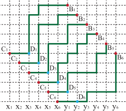
Figure 7: Watermelon with deviation $k=2$ and $N=6$.

It follows from Construction 3.9 that the generating function of watermelons with deviation $k$ is given by the sum:

$$\mathcal{P}_{\mathcal{M}}({\textbf{x}}_{N;k},\textbf{y}_{N}) \equiv\sum\limits_{{\boldsymbol{\lambda}}\subseteq\{{\mathcal{M}}^{N-k}\}}S_{{\boldsymbol{\lambda}}}({\textbf{x}}_{N;k})S_{\widehat{\boldsymbol{\lambda}}}({\textbf{y}}_{N})$$

$$=\sum\limits_{{\boldsymbol{\lambda}}\subseteq\{{\mathcal{M}}^{N-k}\}}\Biggl{(}\sum_{\{{\cal C}_{k}\}}\prod_{x_{j}\in{\bf x}_{N;k}}x_{j}^{c_{j}}\Biggr{)}\Biggl{(}\sum_{\{\cal{B}\}}\prod_{{\alpha}=1}^{N}y_{{\alpha}}^{{\mathcal{M}}-b_{\alpha}}\Biggr{)},$$ (3.30)

where ${\bf x}_{N;k}$ implies either ${\bf x}_{N-k}$ or ${\bf x}_{[N\backslash k]}$. Another representation of the watermelon with deviation may be obtained by gluing the stars ${\cal C}$ and ${\cal B}_{k}$ (see Figure 8), and the generating function reads:

$$\mathcal{P}_{\mathcal{M}}(\textbf{x}_{N},\textbf{y}_{N-k}) \equiv\sum\limits_{{\boldsymbol{\lambda}}\subseteq\{{\mathcal{M}}^{N-k}\}}S_{\widehat{\boldsymbol{\lambda}}}({\textbf{x}}_{N})S_{{\boldsymbol{\lambda}}}({\textbf{y}}_{N-k})$$

$$=\sum\limits_{{\boldsymbol{\lambda}}\subseteq\{{\mathcal{M}}^{N-k}\}}\Biggl{(}\sum_{\{{\cal C}\}}\prod_{j=1}^{N}x_{j}^{c_{j}}\Biggr{)}\Biggl{(}\sum_{\{{\cal{B}}_{k}\}}\prod_{{\alpha}=1}^{N-k}y_{{\alpha}}^{{\mathcal{M}}-b_{\alpha}}\Biggr{)}.$$ (3.31)

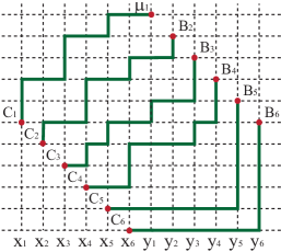
Figure 8: Conjugated watermelon with deviation $k=2$ and $N=6$.

We introduce the generating function ${W}_{q}(N,L,{\mathcal{M}})$ of the watermelons with deviation $k$ by means of

Definition 3.10.

Let a nest ${{\bf w}_{NL{\mathcal{M}}}}$ of $N$ lattice paths characterized by the total numbers $L$ and ${\mathcal{M}}$ of steps along abscissa and ordinate axes to constitute the watermelon with deviation $N-L$. The generating function $W_{q}(N,L,{\mathcal{M}})$ of the nest ${{\bf w}_{NL{\mathcal{M}}}}$ is given by the polynomial

$$W_{q}(N,L,{\mathcal{M}})\equiv\sum_{\{{\bf w}_{NL{\mathcal{M}}}\}}q^{|{\bf w}_{NL{\mathcal{M}}}|_{\delta}},$$ (3.32)

where summation goes over all admissible ${{\bf w}_{NL{\mathcal{M}}}}$. Let $\delta$ to specify the volume of ${\cal C}_{k}$ used in Construction 3.9: the choice $\delta=0$ or $\delta=k$ corresponds to the volume either (3.12) or (3.14). The corresponding volumes $|{{\bf w}_{NL{\mathcal{M}}}}|_{\delta}$ are parameterized by $\delta$:

$$|{\bf w}_{NL{\mathcal{M}}}|_{\delta}\equiv\sum_{j=k+1}^{2N}(2N-j)m_{j}+\delta\sum_{j=k+1}^{N}m_{j}-\frac{{\mathcal{M}}N}{2}(N-1).$$ (3.33)

The numbers of steps along the vertical lines with abscissae $x_{j}$, $k+1\leq j\leq 2N$, respect $\sum_{j=k+1}^{2N}m_{j}={\mathcal{M}}N$ since (3.33) is right-hand side of (3.19) at $m_{1}=m_{2}=\dots=m_{k}=0$ and $k=N-L$.

In the case $N-L=k$, we define the Schur function labelled by $\widehat{\mathbb{M}}$ (3.20) in the form similar to (3.21):

$$S_{\widehat{{\mathbb{M}}}}({\textbf{x}}_{[2N\backslash k]})\equiv\sum_{\{{\bf w}_{NL{\mathcal{M}}}\}}\prod_{j=k+1}^{2N}x_{j}^{m_{j}}.$$ (3.34)

Then the graphical considerations enable to formulate

Proposition 3.11.

The generating function $W_{q}(N,L,{\mathcal{M}})$ (3.32) of watermelons with deviation $N-L=k$ satisfies the identities:

$$W_{q}(N,L,{\mathcal{M}}) =\mathcal{P}_{{\cal M}}\bigg{(}\textbf{q}_{{N;k}},\frac{\textbf{q}_{N}}{q}\bigg{)}$$ (3.35)

$$=q^{-\frac{{\mathcal{M}}N}{2}(N+1)}S_{\widehat{\mathbb{M}}}\bigl{(}\textbf{q}_{N},q^{\delta+N+1},q^{\delta+N+2},\dots,q^{\delta+2N-k}\bigr{)},$$ (3.36)

where $\mathcal{P}_{{\cal M}}\bigl{(}\textbf{q}_{N;k},\textbf{q}_{N}/q\bigr{)}$ and the Schur function $S_{\widehat{\mathbb{M}}}$ are given by (3.30) and (3.34), respectively, under the $q$-parametrization (2.28). The notation $\textbf{q}_{{N;k}}$ implies $\textbf{q}_{N-k}$ at $\delta=0$ or $\textbf{q}_{{N;k}}=\textbf{q}_{[N\backslash k]}$ at $\delta=k$.

Proof.

The volume $|{\bf w}_{NL{\mathcal{M}}}|_{\delta}$ (3.33) respects the relationship

$$|{\cal C}_{k}|_{\rm w}^{\delta}+|{\cal B}|_{\rm w}=|{\bf w}_{NL{\mathcal{M}}}|_{\delta},$$ (3.37)

where $|{\cal B}|_{\rm w}$ is the volume (3.9), and the superscript $\delta$ in $|{\cal C}_{k}|_{\rm w}^{\delta}$ is to stress that either $|{\cal C}_{k}|_{\rm w}$ (3.12) or $|{\cal C}_{k}|_{\overline{\rm w}}$ (3.14) is used at $\delta=0$ or $\delta=k$, respectively. Equations (3.32) and (3.37) lead us to the following relation:

$$W_{q}(N,L,{\mathcal{M}})=\sum_{{\boldsymbol{\lambda}}\subseteq\{{\cal M}^{L}\}}\Biggl{(}\sum_{\{{\cal C}_{k}\}}q^{|{\cal C}_{k}|_{\rm w}^{\delta}}\Biggr{)}\Biggl{(}\sum_{\{{\cal B}\}}q^{|{\cal B}|_{\rm w}}\Biggr{)},$$ (3.38)

since the summation $\sum_{{\boldsymbol{\lambda}}\subseteq\{{\cal M}^{L}\}}\sum_{\{{\cal C}_{k}\}}\sum_{\{{\cal B}\}}$ replaces the sum $\sum_{\{{\bf w}_{NL{\mathcal{M}}}\}}$ (compare with (3.28)). Since the product of (3.10) and (3.13) is expressed as the product of the $q$-parametrized Schur functions, right-hand side of (3.38) is re-expressed:

$$\sum_{{\boldsymbol{\lambda}}\subseteq\{{\cal M}^{L}\}}S_{{\boldsymbol{\lambda}}}(\textbf{q}_{N;k})S_{\widehat{\boldsymbol{\lambda}}}\bigg{(}\frac{\textbf{q}_{N}}{q}\bigg{)}=\mathcal{P}_{{\cal M}}\bigg{(}\textbf{q}_{N;k},\frac{\textbf{q}_{N}}{q}\bigg{)}.$$ (3.39)

Equation (3.35) is valid due to (3.38) and (3.39).

Let us turn to equation (3.36). We obtain from (3.32), (3.33) and (3.34):

$$W_{q}(N,L,{\mathcal{M}})=q^{-\frac{N{\mathcal{M}}}{2}(N-1)+2N^{2}{\mathcal{M}}}S_{\widehat{\mathbb{M}}}\bigg{(}\frac{q^{2\delta-k}}{{\bf q}_{N;k}},\frac{1}{{\bf q}_{[2N\backslash N]}}\bigg{)}.$$ (3.40)

We re-express $W_{q}(N,L,{\mathcal{M}})$ (3.40) at $\delta=0$:

$$W_{q}(N,L,{\mathcal{M}}) =q^{-\frac{N{\mathcal{M}}}{2}(N-1)+2N^{2}{\mathcal{M}}}S_{\widehat{\mathbb{M}}}\bigg{(}\frac{1}{q^{k+1}},\frac{1}{q^{k+2}},\dots,\frac{1}{q^{2N}}\bigg{)}$$

$$=q^{-\frac{N{\mathcal{M}}}{2}(N-1)+(2N-k){\mathcal{M}}N}S_{\widehat{\mathbb{M}}}\bigg{(}\frac{1}{{\bf q}_{2N-k}}\bigg{)}$$

$$=q^{-\frac{{\mathcal{M}}N}{2}(N+1)}S_{\widehat{\mathbb{M}}}({{\bf q}_{2N-k}}).$$ (3.41)

Further, we obtain at $\delta=k$:

$$S_{\widehat{\mathbb{M}}}\bigg{(}\frac{1}{q},\frac{1}{q^{2}},\dots,\frac{1}{q^{N-k}},\frac{1}{q^{N+1}},\dots,\frac{1}{q^{2N}}\bigg{)}$$

$$\qquad{}=q^{-{\mathcal{M}}N(2N+1)}S_{\widehat{\mathbb{M}}}\bigr{(}q^{2N},q^{2N-1},\dots,q^{N+k+1},q^{N},q^{N-1},\dots,q^{2},q\bigl{)}.$$ (3.42)

Equation (3.36) is thus valid due to (3.40) and (3.42). ∎

Corollary.

The Schur function $S_{\widehat{\mathbb{M}}}$ (3.36) acquires the determinantal representation due to Proposition 3.11 provided that (2.29), (2.30), (2.31) are taken into account:

$$S_{\widehat{\mathbb{M}}}\bigl{(}\textbf{q}_{N},q^{\delta+N+1},q^{\delta+N+2},\dots,q^{\delta+N+L}\bigr{)}$$

$$\qquad{}=q^{\frac{{\mathcal{M}}N}{2}(N+1)-\frac{L}{2}(N-L)(2\delta+L-1)}\frac{\det{\overline{T}}^{\delta}}{{\mathcal{V}}({\bf q}_{N}/q){\mathcal{V}}(\mathbf{q}_{N;k})},$$ (3.43)

where the entries of $N\times N$ matrix ${\overline{T}}^{\delta}$ are given:

$${\overline{T}}_{ij}^{\delta}\equiv\frac{[({\mathcal{M}}+N)(\delta+j+i-1)]}{[\delta+j+i-1]},\qquad 1\leq i\leq N-k,\qquad 1\leq j\leq N,$$

$${\overline{T}}_{ij}^{\delta}\equiv q^{j(N-i)},\qquad N-k+1\leq i\leq N,\qquad 1\leq j\leq N.$$ (3.44)

Provided that $k=0$, Proposition 3.11 is reduced to Proposition 3.8 taken at $n=0$.

3.2.3 The generating function $\boldsymbol{W_{q}(N,L,{\mathcal{M}})}$ as determinant

The generating function $W_{q}(N,{\mathcal{M}})$ (3.18) expressed by (3.22) acquires the $q$-binomial determinant form due to (2.36). On the other hand, equation (3.23) represents $W_{q}(N,{\mathcal{M}}/n)$ as the $q$-parameterized Schur function. Although the Schur function representation (3.36) for $W_{q}(N,L,{\mathcal{M}})$ depends on $\delta$, the corresponding limits at $q\to 1$ coincide for $\delta=0$ and $\delta=k$.

The determinantal form of $W_{q}(N,L,{\mathcal{M}})$ at $\delta=0$ is the subject of

Theorem 3.12.

The partition function ${W}_{q}(N,L,{\mathcal{M}})$ of the watermelon with deviation $N-L\allowbreak=k$ respects the determinantal representation:

$${W}_{q}(N,L,{\mathcal{M}}) =q^{-\frac{{\mathcal{M}}N}{2}(N-1)}\det\left(q^{(j-1)({\mathcal{M}}+j-i)}\begin{bmatrix}L+{\mathcal{M}}+N-i\\ {\mathcal{M}}+N-j\end{bmatrix}\right)_{1\leq i,j\leq N}$$ (3.45)

$$=Z_{q}(N,L,{\mathcal{M}})=Z_{q}(L,{\mathcal{M}},N).$$ (3.46)

Proof.

First, the Schur function (2.13) is expressed as a determinant in terms of the complete homogeneous symmetric functions (the Jacobi–Trudi relation, [32, 40, 41]),

$$S_{\widehat{\mathbb{M}}}\bigg{(}\frac{{\bf q}_{2N-k}}{q}\bigg{)}=\det\bigg{(}h_{\mathcal{M}-i+j}\bigg{(}\frac{{\bf q}_{2N-k}}{q}\bigg{)}\bigg{)}_{1\leq i,j\leq N},$$ (3.47)

where the symmetric functions are expressed through the $q$-binomial coefficients (2.26):

$$h_{\mathcal{M}-i+j}\bigg{(}\frac{{\bf q}_{2N-k}}{q}\bigg{)}=\begin{bmatrix}N+L+\mathcal{M}-i+j-1\\ \mathcal{M}-i+j\end{bmatrix}\!.$$ (3.48)

Using (3.48) and the Pascal formula for $q$-binomial coefficients [40, 41], one transforms (3.47):

$$S_{\widehat{\mathbb{M}}}\bigg{(}\frac{{\bf q}_{2N-k}}{q}\bigg{)}=\det\left(q^{(j-1)(\mathcal{M}+j-i)}\begin{bmatrix}\mathcal{M}+N+L-i\\ N+L-j\end{bmatrix}\right)_{1\leq i,j\leq N}\!.$$ (3.49)

Eventually, equation (3.45) is valid due to (3.41) and (3.49). The answer for the partition function $W_{q}(N,\mathcal{M})$ is obtained from (3.45) at $k=0$.

As a next step, we drop the powers of $q^{\mathcal{M}}$, as well as the multiples $[{\mathcal{M}}+L+N-i]$ and $\frac{1}{[L+N-j]}$, $1\leq i,j\leq N$, out of rows and columns of the matrix in right-hand side of (3.49), and obtain:

$$S_{\widehat{{\mathbb{M}}}}\bigg{(}\frac{{\bf q}_{2N-k}}{q}\bigg{)}=q^{\frac{{\mathcal{M}}N}{2}(N-1)}\prod_{i=1}^{N}\prod_{j=1}^{L}\frac{[{\mathcal{M}}+i+j-1]}{[j+i-1]}\det\left(q^{(j-1)(j-i)}\begin{bmatrix}{\mathcal{M}}+N-i\\ N-j\end{bmatrix}\right)_{1\leq i,j\leq N}\!.$$

The determinant in (3.2.3) is calculated iteratively, and unity appears after $N-1$ steps as its value. Therefore, equation (3.46) is valid due to (2.11) and (3.41). ∎

The determinantal representations (2.33) and (3.45) given by Theorems 2.4 and 3.12, respectively, are equivalent and lead to the same double product expressions (2.35) and (3.46), which are interpreted as the generating functions of watermelons. The determinantal representation (3.45) allows to express in the limit $q\rightarrow 1$ the number $A(N,L,{\mathcal{M}})$ of the watermelons with deviation (i.e., the number of plane partitions in ${\cal B}(N,L,{\mathcal{M}})$):

$$A(N,L,{\mathcal{M}})=\det\left(\begin{pmatrix}L+{\mathcal{M}}+N-i\\ {\mathcal{M}}+N-j\end{pmatrix}\right)_{1\leq i,j\leq N}=\prod_{i=1}^{N}\prod_{j=1}^{{\mathcal{M}}}\frac{L+i+j-1}{j+i-1}.$$ (3.50)

Equation (3.50) provides the statement of the Gessel–Viennot theorem [21] that connects the binomial determinant with the number of nests of self-avoiding lattice paths.

The matrix ${\overline{T}}^{\delta}$ (3.44) at $\delta=k$ is simplified in the limit $M\to\infty$ so that the corresponding determinant is tractable. As a result, the partition function ${W}_{q}(N,L,{\mathcal{M}})$ at $\delta=k$ acquires the form of the norm-trace generating function [5] of plane partitions with fixed traces of diagonal parts. The statement is given by the following

Theorem 3.13.

The partition function ${W}_{q}(N,L,{\mathcal{M}})$ of the watermelon with deviation $N-L\allowbreak=k$ expressed by (3.36) at $\delta=k$ takes the form at $M\to\infty$:

$${W}_{q}(N,L,{\mathcal{M}})\underset{M\to\infty}{=}q^{\frac{N-L}{2}(N+L-1)}\prod_{i=1}^{L}\prod_{j=1}^{N}\frac{1}{1-q^{k+i+j-1}}.$$ (3.51)

Proof.

The entries (3.44) at $\delta=k$ are simplified in the limit $M\to\infty$ provided that $q^{kM}\ll 1$:

$${\overline{T}}_{ij}^{\delta=k}=\displaystyle{\frac{1}{1-q^{k+j+i-1}}},\qquad 1\leq i\leq N-k,\qquad 1\leq j\leq N.$$

In order to evaluate $\det{\overline{T}}^{(\delta=k)}$, one firstly combines neighboring rows $i^{\rm th}$ and $(i+1)^{\rm th}$ in (3.44), $L+1\leq i<N$, as required to calculate the Vandermonde determinant. After this, the columns $j^{\rm th}$ and $N^{\rm th}$, $1\leq j<N$, are combined to obtain $N-1$ zeros in $N^{\rm th}$ row. After $N-L$ steps, one obtains:

$$\det{\overline{T}}^{(\delta=k)} =q^{\frac{N}{2}(N-1)+\frac{L}{2}(2N-L-1)(N-L)}\prod_{i=1}^{L}\prod_{j=L+1}^{N}\frac{1}{1-q^{k+i+j-1}}$$

$$\times\frac{\mathcal{V}({\bf q}_{N}/q)}{\mathcal{V}({\bf q}_{L})}\det\bigg{(}\frac{1}{1-q^{k+i+j-1}}\bigg{)}_{1\leq i,j\leq L}\!.$$ (3.52)

The Cauchy determinant in (3.52) is evaluated [5], and one obtains (3.51) from (3.36) provided that (3.52) is used in (3.43). ∎

The representation (3.52) enables the limiting form of the Schur function (3.43).

4 $\boldsymbol{XX}$ Heisenberg chain and dynamical correlation functions

The Heisenberg $XX$ model on a chain of $M+1$ sites is defined by the Hamiltonian:

$$H_{XX}=\frac{{\sf H}}{2}+\frac{1}{2}\sum_{k=0}^{M}(\mathbb{I}-\sigma_{k}^{z}),$$ (4.1)

where $\mathbb{I}$ is identity operator, and the contribution

$${{\sf H}}=-\sum_{n,m=0}^{M}\Delta_{nm}\sigma_{n}^{-}\sigma_{m}^{+}$$ (4.2)

describes the neighbouring spins coupling through the hopping matrix ${\boldsymbol{\Delta}}$,

$${\mathbb{\Delta}}\equiv\bigl{(}\Delta_{nm}\bigr{)}_{0\leq n,m\leq M},\qquad\Delta_{nm}=\delta_{|n-m|,1}+\delta_{|n-m|,M},$$ (4.3)

where $\delta_{kl}\equiv\delta_{k,l}$ is the Kronecker symbol. The entries of ${\mathbb{\Delta}}$ are subjected to the periodicity requirements: $\Delta_{n+M+1,m}=\Delta_{nm}$ and $\Delta_{n,m+M+1}=\Delta_{nm}$. The local spin operators $\sigma^{\pm}_{k}=\frac{1}{2}(\sigma^{x}_{k}\pm{\rm i}\sigma^{y}_{k})$ and $\sigma^{z}_{k}$ act nontrivially on $k^{\rm th}$ site and obey the commutation rules:

$$[\sigma^{+}_{k},\sigma^{-}_{l}]=\delta_{kl}\sigma^{z}_{l},\qquad[\sigma^{z}_{k},\sigma^{\pm}_{l}]=\pm 2\delta_{kl}\sigma^{\pm}_{l}.$$

The spin operators $\sigma^{\pm}_{k}$ and $\sigma^{z}_{k}$ act in the space ${\mathfrak{H}}_{M+1}$ spanned over the states $\bigotimes_{l=0}^{M}|s\rangle_{l}$, where $|s\rangle_{l}$ implies either spin “up”, $\mid\uparrow\rangle$, or spin “down”, $\mid\downarrow\rangle$, state at $l^{\rm th}$ site. The states $\mid\uparrow\rangle\equiv\left(\begin{smallmatrix}1\\ 0\end{smallmatrix}\right)$ and $\mid\downarrow\rangle\equiv\left(\begin{smallmatrix}0\\ 1\end{smallmatrix}\right)$ provide a natural basis of the linear space ${\mathbb{C}}^{2}$. The Hamiltonian (4.1) annihilates the state $\mid\Uparrow\rangle\equiv\bigotimes_{n=0}^{M}\mid\uparrow\rangle_{n}$ with all spins “up”, $H_{XX}\mid\Uparrow\rangle=0$, and commutes with the third component of the total spin ${S}^{z}$:

$$[{H}_{XX},{S}^{z}]=0,\qquad{S}^{z}\equiv\frac{1}{2}\sum_{k=0}^{M}\sigma_{k}^{z}.$$

Consider an arbitrary state on the chain characterized by $N$ spins “down” and ${\mathcal{M}}\equiv M-N+1$ spins “up”. The spin “down” sites are labelled by parts of a strict partition ${{\boldsymbol{\mu}}}=(\mu_{1},\mu_{2},\dots,\mu_{N})$. We define the state $|{\boldsymbol{\mu}}\rangle$ corresponding to $N$ spins “down” and its conjugate $\langle{\boldsymbol{\nu}}|$,

$$|{\boldsymbol{\mu}}\rangle\equiv\Bigg{(}\prod\limits_{k=1}^{N}\sigma_{\mu_{k}}^{-}\Bigg{)}\mid\Uparrow\rangle,\qquad\langle{\boldsymbol{\nu}}|\equiv\langle\Uparrow\mid\Bigg{(}\prod\limits_{k=1}^{N}\sigma_{\nu_{k}}^{+}\Bigg{)},$$ (4.4)

which provide a complete orthogonal base:

$$\langle{\boldsymbol{\nu}}|{\boldsymbol{\mu}}\rangle={\boldsymbol{\delta}}_{{\boldsymbol{\nu}}{\boldsymbol{\mu}}}\equiv\prod\limits_{n=1}^{N}\delta_{\nu_{n}\mu_{n}}.$$ (4.5)

The $N$-particles state-vector $|\Psi({\bf u}_{N})\rangle$ under off-shell parametrization ${\bf u}_{N}$ is the combination of the states (4.4) with the Schur functions $S_{\boldsymbol{\lambda}}({\textbf{u}}^{2}_{N})$ (2.13) as the coefficients:

$$|\Psi({\textbf{u}}_{N})\rangle=\sum\limits_{{\boldsymbol{\lambda}}\subseteq\{{\mathcal{M}}^{N}\}}S_{\boldsymbol{\lambda}}\big{(}{\textbf{u}}^{2}_{N}\big{)}|{\boldsymbol{\mu}}\rangle.$$ (4.6)

The conjugate off-shell state-vectors are given by

$$\langle\Psi({\bf v}_{N})|=\sum\limits_{{\boldsymbol{\lambda}}\subseteq\{{\mathcal{M}}^{N}\}}\langle{\boldsymbol{\nu}}|S_{\boldsymbol{\lambda}}\big{(}{\textbf{v}}^{-2}_{N}\big{)}.$$ (4.7)

Summation in (4.6) and (4.7) goes over the partitions ${\boldsymbol{\lambda}}$ corresponding either to ${\boldsymbol{\mu}}$ or ${\boldsymbol{\nu}}$ (see Section 2 and Figure 1).

The periodic boundary conditions are imposed: $\sigma^{\#}_{k+(M+1)}=\sigma^{\#}_{k}$. If the parameters $u^{2}_{j}\equiv{\rm e}^{{\rm i}\theta_{j}}$ ($1\leq j\leq N$) satisfy the Bethe equations [11],

$${\rm e}^{{\rm i}(M+1)\theta_{j}}=(-1)^{N-1},\qquad 1\leq j\leq N,$$ (4.8)

then the state-vectors (4.6) become the eigen-vectors of the Hamiltonian (4.1):

$${H}_{XX}|\Psi({{\boldsymbol{\theta}}}_{N})\rangle=E_{N}({{\boldsymbol{\theta}}}_{N})|\Psi({{\boldsymbol{\theta}}}_{N})\rangle,$$ (4.9)

where $\big{|}\Psi\big{(}{\rm e}^{\frac{\rm i}{2}{{\boldsymbol{\theta}}}_{N}}\big{)}\big{\rangle}$ is written for simplicity as $|\Psi({{\boldsymbol{\theta}}}_{N})\rangle$. The use of ${{\boldsymbol{\theta}}}$ instead of ${{\boldsymbol{\theta}}}_{N}$ is allowed if there is no confusion. The solutions $\theta_{j}$ to the Bethe equations (4.8) can be parametrized such that

$$\theta_{j}=\frac{2\pi}{M+1}\bigg{(}I_{j}-\frac{N-1}{2}\bigg{)},\qquad 1\leq j\leq N,$$ (4.10)

where $I_{j}$ are integers or half-integers depending on whether $N$ is odd or even.

The eigen-energy in (4.9) is given by

$$E_{N}({{\boldsymbol{\theta}}}_{N})=N-\sum_{j=1}^{N}\cos\theta_{j}=N-\sum_{j=1}^{N}\cos\bigg{(}\frac{2\pi}{M+1}\bigg{(}I_{j}-\frac{N-1}{2}\bigg{)}\bigg{)}.$$ (4.11)

The ground state of the model is the eigen-state determined by (4.10) at $I_{j}=N-j$:

$$\theta^{\rm g}_{j}\equiv\frac{2\pi}{M+1}\bigg{(}\frac{N+1}{2}-j\bigg{)},\qquad 1\leq j\leq N,$$

and the corresponding eigen-energy

$$E_{N}({\boldsymbol{\theta}}^{\rm g}_{N})=N-\csc\bigg{(}\frac{\pi}{M+1}\bigg{)}\sin\bigg{(}\frac{\pi N}{M+1}\bigg{)}.$$

The squared norm of the state vectors (4.6) on the solutions (4.10) is

$${\mathcal{N}}^{2}({{\boldsymbol{\theta}}}_{N})\equiv\langle\Psi({{\boldsymbol{\theta}}}_{N})\mid\!\Psi({{\boldsymbol{\theta}}}_{N})\rangle=\frac{(M+1)^{N}}{|\mathcal{V}({\rm e}^{{\rm i}{{\boldsymbol{\theta}}}_{N}})|^{2}}.$$ (4.12)

Let us introduce two operators,

$$\bar{\varPi}_{n}\equiv\prod\limits_{j=0}^{n-1}\frac{\mathbb{I}+\sigma^{z}_{j}}{2},\qquad\bar{\sf F}_{n}\equiv\prod\limits_{j=0}^{n-1}\sigma^{-}_{j},$$ (4.13)

where $\bar{\varPi}_{n}$ is the projection operator forbidding the spin “down” states on $n$ successive sites, and $\bar{\sf F}_{n}$ is the domain wall operator that creates the spin “down” states on $n$ successive sites. It is assumed that $\bar{\varPi}_{0}$ and $\bar{\sf F}_{0}$ are identity operators.

Let us define the “dynamical” auto-correlation function, which generalizes the correlation functions considered in [3]:

$$\Gamma\big{(}{{\boldsymbol{\theta}}}_{[N\backslash n]}^{\rm g},N,n,m,t_{1},t_{2}\big{)}\equiv\frac{\big{\langle}\Psi\big{(}{{\boldsymbol{\theta}}}^{\rm g}_{[N\backslash n]}\big{)}\big{|}\bar{\sf F}_{n}^{+}{\rm e}^{-t_{1}H_{XX}}{\bar{\varPi}}_{m}{\rm e}^{-t_{2}H_{XX}}\bar{\sf F}_{n}\big{|}\Psi\big{(}{{\boldsymbol{\theta}}}^{\rm g}_{[N\backslash n]}\big{)}\big{\rangle}}{\big{\langle}\Psi\big{(}{{\boldsymbol{\theta}}}^{\rm g}_{[N\backslash n]}\big{)}\big{|}\Psi\big{(}{{\boldsymbol{\theta}}}^{\rm g}_{[N\backslash n]}\big{)}\big{\rangle}},$$ (4.14)

where the operators are given by (4.13), $\bar{\sf F}^{+}_{n}$ is the Hermitian conjugated operator acting on (4.7), and $t_{1}$, $t_{2}$ are the evolution parameters. The states (4.6) and (4.7) in (4.14) are parameterized by elements of $(N-n)$-tuple ${{\boldsymbol{\theta}}}_{[N\backslash n]}^{\rm g}\equiv\big{(}\theta^{\rm g}_{n+1},\theta^{\rm g}_{n+2},\dots,\theta^{\rm g}_{N}\big{)}$ consisting of the ground state solutions to equation (4.8):

$$\theta^{\rm g}_{j}\equiv\frac{2\pi}{M+1}\bigg{(}\frac{N-n+1}{2}-j\bigg{)},\qquad 1\leq j\leq N-n.$$ (4.15)

The persistence of domain wall correlation function arises from (4.14) at $m=0$ and $t=t_{1}+t_{2}$:

$${\cal F}\big{(}{{\boldsymbol{\theta}}}^{\rm g}_{[N\backslash n]},n,t\big{)}\equiv\frac{\big{\langle}\Psi\big{(}{{\boldsymbol{\theta}}}^{\rm g}_{[N\backslash n]}\big{)}\big{|}\bar{\sf F}^{+}_{n}{\rm e}^{-tH_{XX}}\bar{\sf F}_{n}\big{|}\Psi\big{(}{{\boldsymbol{\theta}}}^{\rm g}_{[N\backslash n]}\big{)}\big{\rangle}}{\big{\langle}\Psi\big{(}{{\boldsymbol{\theta}}}^{\rm g}_{[N\backslash n]}\big{)}\big{|}\Psi\big{(}{{\boldsymbol{\theta}}}^{\rm g}_{[N\backslash n]}\big{)}\big{\rangle}},$$ (4.16)

and ${\cal F}\big{(}{{\boldsymbol{\theta}}}^{\rm g}_{[N\backslash n]},0,t\big{)}=1$ since $\bar{\sf F}_{0}$ is identity operator.

5 Random turns vicious walkers and correlations
over ferromagnetic state

In order to interpret the auto-correlation function (4.14) as a sum over nests of self-avoiding lattice paths, we shall firstly pay attention to the correlations over the ferromagnetic state.

Let us turn to description of $N$ vicious walkers [16, 17, 18], which are located initially on a chain at the positions $l_{1}>l_{2}>\cdots>l_{N}$. Two essentially different types of walks of vicious walkers may be distinguished: random turns and lock step walks. Occupation of a site by two walkers is forbidden. In the lock step model at each tick of the clock each walker jumps, with equal probability, to the left or to the right site (see, for instance, Figure 6, where paths connect $C_{i}$ to $B_{i}$, $1\leq i\leq 4$). In the random turns model at each tick only a single randomly chosen walker jumps to right or to left site, whereas the rest are staying (Figure 9). After $K$ steps, the walkers arrive at the positions $j_{1}>j_{2}>\cdots>j_{N}$. Trajectories of the random walkers can be viewed as directed lattice paths (i.e., the paths that can not turn back) on the square lattice.

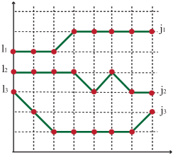
Figure 9: Trajectories of $K=7$ steps for $N=3$ random turns vicious walkers.

We define $N$-particles transition amplitude:

$${\cal G}({\bf j};{\bf l}|t)\equiv\big{\langle}{\bf j}\big{|}{\rm e}^{-tH_{XX}}\big{|}{\bf l}\big{\rangle},$$ (5.1)

where $H_{XX}$ is the Hamiltonian (4.1), and the states $\langle{\bf j}|$ and $|{\bf l}\rangle$ given by (4.4) are respectively labelled by the strict partitions ${\bf j}=(j_{1},j_{2},\dots,j_{N})$ and ${\bf l}=(l_{1},l_{2},\dots,l_{N})$. The generating function of self-avoiding lattice paths of the vicious walkers is enabled by the transition amplitude (5.1):

$$G({\bf j};{\bf l}|t)\equiv\big{\langle}{\bf j}\big{|}{\rm e}^{-\frac{t}{2}{{\sf H}}}\big{|}{\bf l}\big{\rangle}={\rm e}^{tN}{\cal G}({\bf j};{\bf l}|t),$$ (5.2)

where ${{\sf H}}$ is given by (4.2). The condition that vicious walkers do not touch each other up to $N$ steps is guaranteed by the property of the Pauli matrices $(\sigma_{k}^{\pm})^{2}=0$.

Differentiating $G({\bf j};{\bf l}|t)$ (5.2) with respect of $t$ and applying the commutation relation

$$\big{[}{{\sf H}},\sigma_{l_{1}}^{-}\sigma_{l_{2}}^{-}\cdots\sigma_{l_{N}}^{-}\big{]}=\sum_{k=1}^{N}\sigma_{l_{1}}^{-}\cdots\sigma_{l_{k-1}}^{-}[{{\sf H}},\sigma_{l_{k}}^{-}]\sigma_{l_{k+1}}^{-}\cdots\sigma_{l_{N}}^{-},$$ (5.3)

we obtain the equation

$$\frac{\rm d}{{\rm d}t}G({\bf j};{\bf l}|t)=\frac{1}{2}\sum_{k=1}^{N}\bigl{(}G({\bf j};l_{1},l_{2},\dots,l_{k}+1,\dots,l_{N}|t)+G({\bf j};l_{1},l_{2},\dots,l_{k}-1,\dots,l_{N}|t)\bigr{)}$$ (5.4)

(the “final” position ${\bf j}$ is fixed), and a similar equation can be found for fixed ${\bf l}$. The commutation relation

$$[{{\sf H}},\sigma_{m}^{-}]=-\sum_{n=0}^{M}\Delta_{nm}\sigma_{n}^{-}\sigma_{m}^{z},$$ (5.5)

is also used in derivation of (5.4).

The non-intersection condition means that $G({\bf j};{\bf l}|t)=0$ if $l_{k}=l_{p}$ (or $j_{k}=j_{p}$) for any $1\leq k,p\leq N$. Equation (5.4) is supplied with the periodicity requirement in each $j_{k}$, $m_{k}$ with all other $j_{s}$, $m_{s}$ ($k\neq s$) fixed:

$$G(j_{1},j_{2},\dots,j_{k}+M+1,\dots,j_{N};l_{1},l_{2},\dots,l_{N}|t)$$

$$\qquad{}=G(j_{1},j_{2},\dots,j_{N};l_{1},l_{2},\dots,l_{k}+M+1,\dots,l_{N}|t)=G(j_{1},j_{2},\dots,j_{N};l_{1},l_{2},\dots,l_{N}|t).$$

The periodic solution to (5.4) subjected to the “initial condition” $G({\bf j};{\bf l}|0)={\boldsymbol{\delta}}_{{\bf j}{\bf l}}$ (see (4.5)) is given by

Proposition 5.1.

The determinantal representation for solution to equation (5.4) is valid:

$$G(j_{1},j_{2},\dots,j_{N};l_{1},l_{2},\dots,l_{N}|t) =\det\bigl{(}G(j_{r},l_{s}|t)\bigr{)}_{1\leq r,s\leq N}$$

$$=\det\bigl{(}\big{(}{\rm e}^{\frac{t}{2}\mathbb{\Delta}}\big{)}_{j_{r},l_{s}}\bigr{)}_{1\leq r,s\leq N},$$ (5.6)

where $G(j,l|t)$ is given by

$${G}(j,l|t)\equiv\big{\langle}\Uparrow\big{|}\sigma_{j}^{+}{\rm e}^{-\frac{t}{2}{{\sf H}}}\sigma_{l}^{-}\big{|}\Uparrow\big{\rangle}=\bigr{(}{\rm e}^{\frac{t}{2}{\mathbb{\Delta}}}\bigl{)}_{jl}.$$ (5.7)

Proof.

The representation equation (5.6) is derived in [6]. ∎

The determinantal formulae for transition probabilities of $N$ particles are well-known in probability and combinatorics for a long time [21, 24, 25, 31] and still attract attention, e.g., [26, 27].

The unitary matrix $\widehat{\bf u}\equiv(M+1)^{-1/2}\bigl{(}{\rm e}^{{\rm i}l\phi_{s}}\bigr{)}_{0\leq s,l\leq M}$, where $\phi_{s}=\frac{2\pi}{M+1}\bigl{(}s-\frac{M}{2}\bigr{)}$, diagonalizes ${\mathbb{\Delta}}$ (4.3). Therefore the entries (5.7) are:

$$G(j,l|t)\equiv\frac{1}{M+1}\sum\limits_{s=0}^{M}{\rm e}^{{\rm i}\phi_{s}(j-l)+t\cos\phi_{s}}.$$ (5.8)

Using (5.7), (5.8) in (5.6), one obtains another equivalent determinantal solution to (5.4) given by

Proposition 5.2.

Solution to (5.4) is of the form:

$$G({\bf j};{\bf l}|t)=\frac{{\rm e}^{tN}}{(M+1)^{N}}\sum\limits_{\{{\boldsymbol{\phi}}_{N}\}}{\rm e}^{-tE_{N}({\boldsymbol{\phi}}_{N})}\big{|}{\mathcal{V}}({\rm e}^{{\rm i}{\boldsymbol{\phi}}_{N}}\big{)}\big{|}^{2}S_{{{\boldsymbol{\lambda}}^{L}}}\big{(}{\rm e}^{{\rm i}{\boldsymbol{\phi}}_{N}}\big{)}S_{{{\boldsymbol{\lambda}}^{R}}}\big{(}{\rm e}^{-{\rm i}{\boldsymbol{\phi}}_{N}}\big{)},$$ (5.9)

where the sum is over $N$-tuples ${\boldsymbol{\phi}}_{N}=(\phi_{k_{1}},\phi_{k_{2}},\dots,\phi_{k_{N}})$, $\phi_{n}=\frac{2\pi}{M+1}\bigl{(}n-\frac{M}{2}\bigr{)}$ and $M\geq k_{1}>k_{2}\allowbreak>\cdots>k_{N}\geq 0$. The partitions ${{\boldsymbol{\lambda}}^{L}}$, ${{\boldsymbol{\lambda}}^{R}}$ and ${\bf j}$, ${\bf l}$ are related: ${{\boldsymbol{\lambda}}^{L}}={\bf j}-{{\boldsymbol{\delta}}}_{N}$, ${{\boldsymbol{\lambda}}^{R}}={\bf l}-{{\boldsymbol{\delta}}}_{N}$, and ${{\boldsymbol{\delta}}}_{N}$ is (2.3). Besides, the Vandermonde deteminant ${\mathcal{V}}({\rm e}^{{\rm i}{\boldsymbol{\phi}}_{N}})$, where ${\rm e}^{\pm{\rm i}{\boldsymbol{\phi}}_{N}}\equiv({\rm e}^{\pm{\rm i}\phi_{1}},{\rm e}^{\pm{\rm i}\phi_{2}},\dots,{\rm e}^{\pm{\rm i}\phi_{N}})$, is defined by (2.14), and $E_{N}({\boldsymbol{\phi}}_{N})$ is defined by (4.11).

Proof.

The representation equation (5.9) is derived in [3]. ∎

Expanding the representation (5.2) in powers of $t$, we obtain the series

$$G({\bf j};{\bf l}|t)=\sum_{K=0}^{\infty}\frac{(t/2)^{K}}{K!}\mathfrak{G}({\bf j};{\bf l}|K),$$ (5.10)

where the coefficients are the averages:

$$\mathfrak{G}({\bf j};{\bf l}|K)\equiv\big{\langle}{\bf j}\big{|}(-{{\sf H}})^{K}\big{|}{\bf l}\big{\rangle}.$$ (5.11)

Let us define $N$-tuples ${\bf e}_{k}$, $1\leq k\leq N$, consisting of zeros except a unity at $k^{\rm th}$ place (say, from left). The commutation relation (5.5) allows to establish that $\mathfrak{G}({\bf j};{\bf l}|K)$ (5.11) satisfies the identity:

$$\mathfrak{G}({\bf j};{\bf l}|K+1)=\sum_{k=1}^{N}\bigl{(}\mathfrak{G}({\bf j};{\bf l}+{\bf e}_{k}|K)+\mathfrak{G}({\bf j};{\bf l}-{\bf e}_{k}|K)\bigr{)}.$$ (5.12)

Solution to (5.12) takes the form [6]:

$$\mathfrak{G}(j_{1},j_{2},\dots,j_{N};l_{1},l_{2},\dots,l_{N}|K)=\sum_{|{\bf k}|=K}P({\bf k})\det\bigl{(}\big{(}\mathbb{\Delta}^{k_{r}}\big{)}_{j_{r},l_{s}}\bigr{)}_{1\leq r,s\leq N},$$ (5.13)

where $|{\bf k}|\equiv k_{1}+k_{2}+\cdots+k_{N}$, and $P({\bf k})$ is the multinomial coefficient:

$$P({\bf k})\equiv\frac{(k_{1}+k_{2}+\cdots+k_{N})!}{k_{1}!k_{2}!\cdots k_{N}!}.$$

Let $|P_{K}({\bf l}\rightarrow{\bf j})|$ be the number of $K$-step paths traced by $N$ vicious walkers in the random turns model [16]. From (5.13) it is clear, [6], that equation (5.11) provides us the number of configurations of $N$ random turns walkers being initially located on the sites $l_{1}>l_{2}>\dots>l_{N}$ and arrived after $K$ steps at the positions $j_{1}>j_{2}>\cdots>j_{N}$:

$$|P_{K}({\bf l}\rightarrow{\bf j})|=\mathfrak{G}({\bf j};{\bf l}|K).$$ (5.14)

The $N$-particles transition amplitude (5.1) arises from (5.2), where (5.6) or (5.9) are used.

6 Two-time correlations over ferromagnetic state

Before studying (4.14), let us consider, by analogy with ${\cal G}({\bf j};{\bf l}|t)$ (5.1) and $G({\bf j};{\bf l}|t)$ (5.2), “two-time” transition amplitude,

$${\cal G}({\bf j};{\bf l}|t_{1},t_{2},m)\equiv\big{\langle}{\bf j}\big{|}{\rm e}^{-{t_{1}}H_{XX}}{\bar{\varPi}}_{m}{\rm e}^{-{t_{2}}H_{XX}}\big{|}{\bf l}\big{\rangle},$$ (6.1)

and “two-time” generating function of self-avoiding lattice paths:

$${G}({\bf j};{\bf l}|t_{1},t_{2},m)\equiv\big{\langle}{\bf j}\big{|}{\rm e}^{-\frac{t_{1}}{2}{{\sf H}}}{\bar{\varPi}}_{m}{\rm e}^{-\frac{t_{2}}{2}{{\sf H}}}\big{|}{\bf l}\big{\rangle}={\rm e}^{(t_{1}+t_{2})N}{\cal G}({\bf j};{\bf l}|t_{1},t_{2},m).$$ (6.2)

As in Section 5, differentiating (6.2) with respect to $t_{1}$ and $t_{2}$ and using the commutation relations (5.3), (5.5) we obtain the difference-differential equation:

$$\frac{\partial^{2}}{\partial t_{1}\partial t_{2}}{G}({\bf j};{\bf l}|t_{1},t_{2},m)$$

$$\qquad{}=\frac{1}{4}\sum_{f,p=1}^{N}\sum_{s,s^{\prime}=\pm 1}{G}(j_{1},\dots,j_{f}+s,\dots,j_{N};l_{1},\dots,l_{p}+s^{\prime},\dots,l_{N}|t_{1},t_{2},m).$$ (6.3)

Equation (6.3) is supplied with the “initial condition”: $G({\bf j};{\bf l}|0,0,m)=\prod_{p=1}^{N}\delta_{j_{p},l_{p}}$ provided that $j_{p},l_{p}\geq m$, $\forall p$.

Let us first consider the simplest “two-time” generating function:

$${G}(j,l|t_{1},t_{2},m)\equiv\big{\langle}\Uparrow\big{|}\sigma_{j}^{+}{\rm e}^{-\frac{t_{1}}{2}{{\sf H}}}{\bar{\varPi}}_{m}{\rm e}^{-\frac{t_{2}}{2}{{\sf H}}}\sigma_{l}^{-}\big{|}\Uparrow\big{\rangle}.$$ (6.4)

We derive the difference-differential equation differentiating (6.4) and applying the commutation relation (5.5):

$$\frac{\partial^{2}}{\partial t_{1}\partial t_{2}}{G}(j,l|t_{1},t_{2},m)={} \frac{1}{4}\bigl{(}{G}(j+1,l+1|t_{1},t_{2},m)+{G}(j+1,l-1|t_{1},t_{2},m)$$

$$+{G}(j-1,l+1|t_{1},t_{2},m)+{G}(j-1,l-1|t_{1},t_{2},m)\bigr{)}.$$ (6.5)

As far as the “initial” conditions are concerned, we obtain from (6.4) that ${G}\left(j,l|t_{1},t_{2},m\right)$ vanishes at $t_{1}=t_{2}=0$ for $j$, $l$ respecting $0\leq j,l<m$. Otherwise, ${G}(j,l|0,0,m)=\delta_{jl}$. The solution to (6.5) is of the form

$${G}(j,l|t_{1},t_{2},m)=\sum_{k=m}^{M}{G}(j,k|t_{1}){G}(k,l|t_{2}),$$ (6.6)

where ${G}(j,l|t)$ is the solution (5.8). We obtain from (6.6) at $m=0$:

$${G}(j,l|t_{1},t_{2},0)={G}(j,l|t_{1}+t_{2}),$$

in agreement with (5.7) and (6.4).

Regarding (6.6), we arrive at

Proposition 6.1.

Solution to equation $(\ref{twop9})$ takes the form:

$${G}({\bf j};{\bf l}|t_{1},t_{2},m)=\sum_{\boldsymbol{\rho}\subseteq\{({\cal M}/m)^{N}\}}{G}({\bf j};{\boldsymbol{\rho}}+{{\boldsymbol{\delta}}}_{N}|t_{1}){G}({\boldsymbol{\rho}}+{{\boldsymbol{\delta}}}_{N};{\bf l}|t_{2}),$$ (6.7)

where ${G}({\bf j};{\boldsymbol{\rho}}+{{\boldsymbol{\delta}}}_{N}|t_{1,2})$ are given by $(\ref{ratbe7})$.

Proof.

It is straightforward to verify that solution to (6.3) can be written as

$${G}({\bf j};{\bf l}|t_{1},t_{2},m)=\det({G}(j_{k},l_{n}|t_{1},t_{2},m))_{1\leq k,n\leq N},$$ (6.8)

where the entries ${G}(j_{k},l_{n}|t_{1},t_{2},m)$ given by (6.6) correspond to the product of two rectangular matrices. Application of the Cauchy–Binet formula for matrices enables to arrive from (6.8) to (6.7). Taking into account that the entries ${G}(j_{k},l_{n}\mid t)$ are of the form (5.8), one arrives at (6.7), where ${G}({\bf j};{\bf l}\mid t)$ is given by (5.9). ∎

Expanding (6.2) in double series with respect of $\bigl{(}\frac{t_{1}}{2}\bigr{)}^{K_{1}}$ and $\bigl{(}\frac{t_{2}}{2}\bigr{)}^{K_{2}}$, one obtains the coefficients expressed by the average:

$${\mathfrak{G}}({\bf j};{\bf l}|K_{1},K_{2},m)\equiv\big{\langle}{\bf j}\big{|}(-{{\sf H}})^{K_{1}}{\bar{\varPi}}_{m}(-{{\sf H}})^{K_{2}}\big{|}{\bf l}\big{\rangle}.$$ (6.9)

Applying (5.5), we obtain that ${\mathfrak{G}}({\bf j};{\bf l}|K_{1},K_{2},m)$ (6.9) satisfies the identity:

$${\mathfrak{G}}({\bf j};{\bf l}|K_{1}+1,K_{2}+1,m)=\sum_{f,p=1}^{N}\sum_{s,s^{\prime}=\pm 1}{\mathfrak{G}}({\bf j}+s{\bf e}_{f};{\bf l}+s^{\prime}{\bf e}_{p}|K_{1},K_{2},m),$$ (6.10)

where ${\bf e}_{p,f}$ are the same as in (5.12). Using (5.10) in (6.7), we obtain the representation:

$${\mathfrak{G}}({\bf j};{\bf l}|K_{1},K_{2},m)=\sum_{\boldsymbol{\rho}\subseteq\{({\cal M}/m)^{N}\}}{\mathfrak{G}}({\bf j};{\boldsymbol{\rho}}+{{\boldsymbol{\delta}}}_{N}|K_{1}){\mathfrak{G}}({\boldsymbol{\rho}}+{{\boldsymbol{\delta}}}_{N};{\bf l}|K_{2}).$$ (6.11)

Since ${\mathfrak{G}}({\bf j};{\bf l}|K)$ (5.11) fulfils (5.12), it is straightforward to check that (6.11) fulfils (6.10).

As in the case of equation (5.11), the average ${\mathfrak{G}}({\bf j};{\bf l}|K_{1},K_{2},m)$ (6.9) enumerates the nests of $(K_{1}+K_{2})$-step paths connecting the sites constituting ${\bf j}$ and ${\bf l}$:

$$\big{|}P_{K_{1}+K_{2}}({\bf l}\underset{m}{\rightarrow}{\bf j})\big{|}\equiv{\mathfrak{G}}({\bf j};{\bf l}|K_{1},K_{2},m),$$ (6.12)

where the notation in left-hand side is a modification of the notation (5.14). Indeed, equation (6.11) is re-expressed regarding (5.14) and (6.12) as follows:

$$\big{|}P_{K_{1}+K_{2}}({\bf l}\underset{m}{\rightarrow}{\bf j})\big{|}=\sum_{\boldsymbol{\rho}\subseteq\{({\cal M}/m)^{N}\}}|P_{K_{1}}({\bf l}\rightarrow{\boldsymbol{\rho}}+{{\boldsymbol{\delta}}}_{N})||P_{K_{2}}({\boldsymbol{\rho}}+{{\boldsymbol{\delta}}}_{N}\rightarrow{\bf j})|.$$ (6.13)

The representation (6.13) demonstrates that (6.12) enumerates the nests of such paths, which are due to “gluing” of the directed paths ${\bf l}\rightarrow{\boldsymbol{\rho}}+{{\boldsymbol{\delta}}}_{N}$ to the directed paths ${\boldsymbol{\rho}}+{{\boldsymbol{\delta}}}_{N}\rightarrow{\bf j}$, as depicted in Figure 9. The “gluing” is along a “dissection” line characterized by the strict partition ${\boldsymbol{\rho}}+{{\boldsymbol{\delta}}}_{N}$ provided that visiting the sites from $0^{\rm th}$ to $(m-1)^{\rm th}$ is forbidden. Therefore, $\big{|}P_{K_{1}+K_{2}}({\bf l}\underset{m}{\rightarrow}{\bf j})\big{|}$ (6.12) enumerates the random turns walks constrained by a bottleneck. The bottleneck is absent if $m=0$, and (6.11) is reduced to the coefficient corresponding to $K=K_{1}+K_{2}$ of the correlation function (5.6) with $t=t_{1}+t_{2}$.

7 Correlations over $\boldsymbol{N}$-particles ground state

This section is devoted to $N$-particles correlation functions (4.14) and (4.16).

7.1 Form-factors of the operators $\boldsymbol{{\bar{\varPi}}_{m}}$ and $\boldsymbol{\bar{\sf F}_{n}}$

Form-factor of the projector $\bar{\varPi}_{m}$ (4.13) is defined as the average

$$\mathcal{T}({\textbf{v}_{N}},{\textbf{u}_{N}},m)\equiv\big{\langle}\Psi({\textbf{v}_{N}})\big{|}\bar{\varPi}_{m}\big{|}\Psi({\textbf{u}_{N}})\big{\rangle},$$ (7.1)

where ${\textbf{u}_{N}}$ and ${\textbf{v}_{N}}$ are $N$-tuples of arbitrary complex numbers. Equations (4.6) and (4.7) allow us to calculate (7.1), and the answer is obtained in terms of the Cauchy–Binet identity (2.16):

$$\mathcal{T}({\textbf{v}_{N}},{\textbf{u}_{N}},m)=\mathcal{P}_{{\mathcal{M}}/m}\big{(}{\textbf{v}}^{-2}_{N},{\textbf{u}}^{2}_{N}\big{)}=\Bigg{(}\prod\limits_{l=1}^{N}\frac{u_{l}^{2m}}{v_{l}^{2m}}\Bigg{)}\frac{\det(T_{kj})_{1\leq k,j\leq N}}{{\mathcal{V}}({\textbf{u}}_{N}^{2}){\mathcal{V}}({\textbf{v}}^{-2}_{N})},$$ (7.2)

where $T_{kj}$ are given by (2.17) with ${\cal L}$ replaced by ${\mathcal{M}}$. Equation (7.2) (together with (3.17)) demonstrates that (7.1) is interpreted as a sum of the watermelons defined by Construction 3.6 (Section 3.2). However, the watermelons are constrained since summation in $\mathcal{P}_{{\mathcal{M}}/m}$ (7.2) is restricted from below, $\mu_{N}\geq m$, and the lattice paths are infiltrating above the column of height $m$ in the middle of Figure 6($a$). For $m=0$, equation (7.2) expresses the scalar product.

Under the $q$-parameterization

$${\bf v}_{N}^{-2}={\bf q}_{N}\equiv\big{(}q,q^{2},\dots,q^{N}\big{)},\qquad{\bf u}_{N}^{2}={\bf q}_{N}/q=\big{(}1,q,\dots,q^{N-1}\big{)},$$ (7.3)

the form-factor (7.1) takes the form:

$$\mathcal{T}\big{(}{\textbf{q}_{N}^{-\frac{1}{2}}},(\textbf{q}_{N}/q)^{\frac{1}{2}},m\big{)} =\mathcal{P}_{\mathcal{M}/m}(\textbf{q}_{N},\textbf{q}_{N}/q)=q^{mN^{2}}W_{q}(N,{\cal M}-m)$$

$$=q^{mN^{2}}Z_{q}(N,N,{\mathcal{M}}-m),$$ (7.4)

where the definition (3.18) and Proposition 3.8 (see (3.27), (3.29)) are used together with (2.18) and (2.37). It is seen from (7.4) that $q$-parametrized form-factor of $\bar{\varPi}_{m}$ is the generating function $W_{q}(N,{\cal M}-m)$ of constrained watermelons or, equivalently, is the generating function $Z_{q}(N,N,{\mathcal{M}}-m)$ of boxed plane partitions in ${\cal B}(N,N,{\mathcal{M}}-m)$ (see (2.38) and Figure 6):

$$\lim\limits_{q\to 1}{\mathcal{T}}\big{(}{\textbf{q}}_{N}^{-\frac{1}{2}},(\textbf{q}_{N}/q)^{\frac{1}{2}},m\big{)}=A(N,N,{\mathcal{M}}-m).$$ (7.5)

Let us turn to the form-factor of the domain wall annihilation operator $\bar{\sf F}_{n}^{+}$ (4.13):

$${\cal F}\big{(}\textbf{v}_{[N\backslash n]},\textbf{u}_{N},n\big{)}\equiv\big{\langle}\Psi\big{(}{\bf v}_{[N\backslash n]}\big{)}\big{|}\bar{\sf F}_{n}^{+}\big{|}\Psi({\bf u}_{N})\big{\rangle},$$ (7.6)

where (2.10) is taken into account. First, let us act by $\bar{\sf F}_{n}^{+}$ (4.13) on the state (4.7):

$$\big{\langle}\Psi\big{(}{\bf v}_{[N\backslash n]}\big{)}\big{|}\bar{\sf F}_{n}^{+} =\sum_{{{\boldsymbol{\eta}}}\subseteq\{({\mathcal{M}}+n)^{N-n}\}}\big{\langle}{{\boldsymbol{\nu}}}_{N-n}\big{|}S_{{{\boldsymbol{\eta}}}}\big{(}{\textbf{v}}^{-2}_{[N\backslash n]}\big{)}\bar{\sf F}_{n}^{+}$$ (7.7)

$$=\sum_{{{\boldsymbol{\eta}}}\subseteq\{{(({\mathcal{M}}+n)/n)}^{N-n}\}}\big{\langle}{{{\boldsymbol{\nu}}}_{N-n},{\boldsymbol{\delta}}_{n}}\big{|}S_{{{\boldsymbol{\eta}}}}\big{(}{\textbf{v}}^{-2}_{[N\backslash n]}\big{)}$$ (7.8)

$$=\Bigg{(}\prod\limits_{l=n+1}^{N}v^{-2n}_{l}\Bigg{)}\sum_{{{\boldsymbol{\eta}}}\subseteq\{{\mathcal{M}}^{N-n}\}}\big{\langle}{\widehat{\boldsymbol{\nu}}}\big{|}S_{{{{\boldsymbol{\eta}}}}}\big{(}{\textbf{v}}^{{-2}}_{[N\backslash n]}\big{)},$$ (7.9)

where ${\widehat{\boldsymbol{\nu}}}=({{\boldsymbol{\nu}}}_{N-n}+{\bf n}_{N-n},{\boldsymbol{\delta}}_{n})$ (see (2.5)). The parts of ${\boldsymbol{\nu}}_{N-n}$ respect $M\geq\nu_{1}>\nu_{2}>\cdots>\nu_{N-n}\geq 0$ in (7.7), or $M\geq\nu_{1}>\nu_{2}>\cdots>\nu_{N-n}\geq n$ in (7.8), or $M-n\geq\nu_{1}>\nu_{2}>\cdots>\nu_{N-n}\geq 0$ in (7.9); in all three cases summation is over non-strict partitions ${\boldsymbol{\eta}}_{N-n}={\boldsymbol{\nu}}_{N-n}-{\boldsymbol{\delta}}_{N-n}$. The state in (7.9) and its conjugate are defined:

$$\big{\langle}{\widehat{{\boldsymbol{\nu}}}}\big{|}\equiv\langle\Uparrow\mid\Bigg{(}\prod\limits_{l=1}^{N-n}\sigma_{n+\nu_{l}}^{+}\Bigg{)}\prod\limits_{l=0}^{n-1}\sigma_{l}^{+},\qquad\big{|}{\widehat{{\boldsymbol{\mu}}}}\big{\rangle}\equiv\prod\limits_{p=1}^{N-n}\sigma_{n+\mu_{p}}^{-}\Bigg{(}\prod\limits_{l=0}^{n-1}\sigma_{l}^{-}\Bigg{)}\mid\Uparrow\rangle.$$ (7.10)

One obtains from (7.9) the transition amplitude interpreted as a sum of the stars with deviation $n$ (Figure 4):

$$\big{\langle}\Psi\big{(}{\bf v}_{[N\backslash n]}\big{)}\big{|}\bar{\sf F}_{n}^{+}|\widehat{{\boldsymbol{\mu}}}\rangle=\Bigg{(}\prod\limits_{l=n+1}^{N}v^{-2n}_{l}\Bigg{)}S_{{{\boldsymbol{\lambda}}}}\big{(}{\bf v}^{-2}_{[N\backslash n]}\big{)}=\sum_{\{{\cal C}_{n}\}}\prod_{j=n+1}^{N}v^{-2(c_{j}+n)}_{j},$$ (7.11)

where (3.11) is taken into account, and ${{\boldsymbol{\lambda}}}\equiv{{\boldsymbol{\lambda}}}_{N-n}$ is given by $\widehat{\boldsymbol{\lambda}}$ in accord with (2.4), (2.5). The transition amplitude of the domain wall creation operator $\bar{\sf F}_{n}$ calculated with the help of (2.23) and (3.16) is a sum of the stars in Figure 5:

$$\big{\langle}\widehat{{\boldsymbol{\mu}}}\big{|}\bar{\sf F}_{n}\big{|}\Psi({\bf u}_{N-n})\big{\rangle}=\Bigg{(}\prod\limits_{l=1}^{N-n}u^{2n}_{l}\Bigg{)}S_{{{\boldsymbol{\lambda}}}}\big{(}\mathbf{u}_{N-n}^{2}\big{)}=\sum_{\{{\cal B}_{n}\}}\prod_{l=1}^{N-n}u_{l}^{2(b_{l}+n)},$$ (7.12)

where ${{\boldsymbol{\lambda}}}$ and $\widehat{{\boldsymbol{\mu}}}$ are the same as in (7.11).

The averages (7.11) and (7.12) are specified for $|\widehat{{\boldsymbol{\mu}}}\rangle=\big{|}\widehat{{\boldsymbol{\delta}}}_{N}\big{\rangle}$, $\langle\widehat{{\boldsymbol{\mu}}}|=\big{\langle}\widehat{{\boldsymbol{\delta}}}_{N}\big{|}$:

$$\big{\langle}\Psi\big{(}{\bf v}_{[N\backslash n]}\big{)}\big{|}\bar{\sf F}_{n}^{+}\big{|}\widehat{{\boldsymbol{\delta}}}_{N}\big{\rangle}=\prod_{j=n+1}^{N}v^{-2n}_{j},\qquad\big{\langle}\widehat{{\boldsymbol{\delta}}}_{N}\big{|}\bar{\sf F}_{n}\big{|}\Psi({\bf u}_{N-n})\big{\rangle}=\prod_{l=1}^{N-n}u_{l}^{2n}.$$ (7.13)

The stars, Figure 4 or Figure 5, correspond to ratios of (7.11) or (7.12) to appropriately chosen average (7.13).

Using the definitions of the state-vectors (4.6) and (4.7) we obtain that the form-factor (7.6),

$${\cal F}\big{(}\textbf{v}_{[N\backslash n]},\textbf{u}_{N},n\big{)} =\Bigg{(}\prod\limits_{l=n+1}^{N}v^{-2n}_{l}\Bigg{)}\sum\limits_{{\boldsymbol{\lambda}}\subseteq\{{\mathcal{M}}^{N-n}\}}S_{{\boldsymbol{\lambda}}}\big{(}{\textbf{v}}^{-2}_{[N\backslash n]}\big{)}S_{\widehat{\boldsymbol{\lambda}}}\big{(}{\textbf{u}}_{N}^{2}\big{)}$$

$$=\Bigg{(}\prod\limits_{l=n+1}^{N}v^{-2n}_{l}\Bigg{)}\mathcal{P}_{\mathcal{M}}\big{(}\textbf{v}_{[N\backslash n]}^{-2},\textbf{u}_{N}^{2}\big{)},$$ (7.14)

is equal, up to pre-factor, to the generator of watermelons with deviation (3.30). Analogously,

$${\cal F}(\textbf{v}_{N},\textbf{u}_{N-n},n)=\Bigg{(}\prod\limits_{l=1}^{N-n}u^{2n}_{l}\Bigg{)}\mathcal{P}_{\mathcal{M}}\big{(}{\textbf{v}}^{-2}_{N},{\textbf{u}}^{2}_{N-n}\big{)},$$ (7.15)

where $\mathcal{P}_{\mathcal{M}}\big{(}{\textbf{v}}^{-2}_{N},{\textbf{u}}^{2}_{N-n}\big{)}$ corresponds to (3.17). Application of Theorem 2.2 leads to the determinantal representations of the form-factors (7.14) and (7.15).

According to Theorem 2.4, the representation, for instance, (7.15) taken in the $q$-parametrization (7.3) is the generating function of plane partitions in the box ${\cal B}(N-n,N,{\mathcal{M}})$ (see (2.35)):

$${\cal F}\bigl{(}{\bf q}_{N}^{-\frac{1}{2}},({\bf q}_{N-n}/q)^{\frac{1}{2}},n\bigr{)} =q^{\frac{n}{2}(N-n)(N-n-1)}{{\mathcal{P}}_{\mathcal{M}}}({\bf q}_{N-n}/q,{\bf q}_{N})$$

$$=q^{\frac{n}{2}(N-n)(N-n-1)}Z_{q}(N-n,N,{\mathcal{M}}).$$

The number of plane partitions confined in this box (i.e., of watermelons with deviation) is given by

$$\lim\limits_{q\to 1}{\cal F}\bigl{(}{\bf q}_{N}^{-\frac{1}{2}},({\bf q}_{N-n}/q)^{\frac{1}{2}},n\bigr{)}=A(N-n,N,{\mathcal{M}}).$$ (7.16)

7.2 Persistence of domain wall

Let us turn to the persistence of domain wall (4.16):

$${\cal F}\big{(}{{\boldsymbol{\theta}}}^{\rm g}_{[N\backslash n]},n,t\big{)}={\rm e}^{-tN}\frac{\big{\langle}\Psi\big{(}{{\boldsymbol{\theta}}}^{\rm g}_{[N\backslash n]}\big{)}\big{|}\bar{\sf F}^{+}_{n}{\rm e}^{-\frac{t}{2}{{\sf H}}}\bar{\sf F}_{n}\big{|}\Psi\big{(}{{\boldsymbol{\theta}}}^{\rm g}_{[N\backslash n]}\big{)}\big{\rangle}}{\big{\langle}\Psi\big{(}{{\boldsymbol{\theta}}}^{\rm g}_{[N\backslash n]}\big{)}\big{|}\Psi\big{(}{{\boldsymbol{\theta}}}^{\rm g}_{[N\backslash n]}\big{)}\big{\rangle}},$$ (7.17)

where $N$ is the number of spins “down”, ${{\boldsymbol{\theta}}}^{\rm g}_{[N\backslash n]}$ is $(N-n)$-tuple of solutions (4.15), and ${{\sf H}}$ is given by (4.2).

The combinatorial properties we are interested in are expressed by the average in the numerator of (7.17) taken under off-shell parametrization. Due to orthogonality of the states $|{\boldsymbol{\mu}}_{N}\rangle$ at fixed $N$, equations (7.11) and (7.12) lead us to the representation [4]:

$$\big{\langle}\Psi\big{(}{\bf v}_{[N\backslash n]}\big{)}\big{|}\bar{\sf F}_{n}^{+}{\rm e}^{-\frac{t}{2}{{\sf H}}}\bar{\sf F}_{n}\big{|}\Psi({\bf u}_{N-n})\big{\rangle}$$

$$\qquad{}=\Bigg{(}\prod\limits_{l=1}^{N-n}\frac{u^{2n}_{l}}{v^{2n}_{l+n}}\Bigg{)}\sum\limits_{{{\boldsymbol{\lambda}}^{L,R}}\subseteq\{{\mathcal{M}}^{N-n}\}}S_{{{\boldsymbol{\lambda}}^{L}}}\big{(}{\bf v}_{[N\backslash n]}^{-2}\big{)}S_{{{\boldsymbol{\lambda}}^{R}}}\big{(}{\textbf{u}}_{N-n}^{2}\big{)}G\big{(}{\widehat{{\boldsymbol{\mu}}}^{L}};{\widehat{{\boldsymbol{\mu}}}^{R}}\big{|}t\big{)},$$ (7.18)

where ${\textbf{u}}^{2}_{N-n}$ and ${\textbf{v}}^{2}_{[N\backslash n]}$ stand for off-shell parameterization, and summations go over partitions ${{\boldsymbol{\lambda}}}^{R,L}$, $l({{\boldsymbol{\lambda}}}^{R,L})=N-n$. The corresponding strict partitions ${{\boldsymbol{\mu}}}^{R,L}={{\boldsymbol{\mu}}}^{R,L}_{N-n}={{\boldsymbol{\lambda}}}^{R,L}_{N-n}+{{\boldsymbol{\delta}}}_{N-n}$ respect

$$M-n\geq\mu_{1}^{R,L}>\mu_{2}^{R,L}>\cdots>\mu_{N-n}^{R,L}\geq 0.$$ (7.19)

The correlation function $G\big{(}{\widehat{{\boldsymbol{\mu}}}^{L}};{\widehat{{\boldsymbol{\mu}}}^{R}}\big{|}t\big{)}$ in (7.18) is defined by (5.2),

$$G\big{(}{\widehat{{\boldsymbol{\mu}}}^{L}};{\widehat{{\boldsymbol{\mu}}}^{R}}\big{|}t\big{)}=\big{\langle}{\widehat{{\boldsymbol{\mu}}}^{L}}\big{|}{\rm e}^{-\frac{t}{2}{{\sf H}}}\big{|}{\widehat{{\boldsymbol{\mu}}}^{R}}\big{\rangle},$$

where $\big{\langle}{\widehat{{\boldsymbol{\mu}}}^{L}}\big{|}$ and $\big{|}{\widehat{{\boldsymbol{\mu}}}^{R}}\big{\rangle}$ are given by (7.10). The partitions ${\widehat{{\boldsymbol{\mu}}}^{L,R}}$ are of length $l\big{(}{\widehat{{\boldsymbol{\mu}}}^{L,R}}\big{)}=N$, and their parts are related with those of ${{\boldsymbol{\mu}}}^{R,L}$, which respect (7.19) (see (2.4) and (2.5)):

$$\big{(}{\widehat{\mu}_{1}^{L,R}},{\widehat{\mu}^{L,R}}_{2},\dots,{\widehat{\mu}^{L,R}}_{N}\big{)} \equiv\big{(}{{\boldsymbol{\mu}}}_{N-n}^{L,R}+{\bf n}_{N-n},{{\boldsymbol{\delta}}}_{n}\big{)}$$

$$\equiv\big{(}{\mu_{1}^{L,R}+n},{\mu_{2}^{L,R}+n},\dots,{\mu_{N-n}^{L,R}+n},n-1,n-2,\dots,1,0\big{)}.$$

Expanding the exponential in (7.18), we obtain:

$$\big{\langle}\Psi\big{(}{\bf v}_{[N\backslash n]}\big{)}\big{|}\bar{\sf F}_{n}^{+}{\rm e}^{-\frac{t}{2}{{\sf H}}}\bar{\sf F}_{n}\big{|}\Psi({\bf u}_{N-n})\big{\rangle}=\sum_{K=0}^{\infty}\frac{(t/2)^{K}}{K!}\big{\langle}\Psi\big{(}{\bf v}_{[N\backslash n]}\big{)}\big{|}\bar{\sf F}_{n}^{+}{(-{{\sf H}})^{K}}\bar{\sf F}_{n}\big{|}\Psi({\bf u}_{N-n})\big{\rangle},$$

where

$$\big{\langle}\Psi\big{(}{\bf v}_{[N\backslash n]}\big{)}\big{|}\bar{\sf F}_{n}^{+}{(-{{\sf H}})^{K}}\bar{\sf F}_{n}\big{|}\Psi({\bf u}_{N-n})\big{\rangle}$$

$$\qquad{}=\Bigg{(}\prod\limits_{l=1}^{N-n}\frac{u^{2n}_{l}}{v^{2n}_{l+n}}\Bigg{)}\sum\limits_{{{{\boldsymbol{\lambda}}}^{L,R}}\subseteq\{{\mathcal{M}}^{N-n}\}}S_{{{{\boldsymbol{\lambda}}}^{L}}}\big{(}{\bf v}_{[N\backslash n]}^{-2}\big{)}S_{{{{\boldsymbol{\lambda}}}^{R}}}\big{(}{\textbf{u}}_{N-n}^{2}\big{)}\mathfrak{G}\big{(}{\widehat{{\boldsymbol{\mu}}}^{L}};{\widehat{{\boldsymbol{\mu}}}^{R}}\big{|}K\big{)}.$$ (7.20)

The coefficient $\mathfrak{G}\big{(}{\widehat{{\boldsymbol{\mu}}}^{L}};{\widehat{{\boldsymbol{\mu}}}^{R}}\big{|}K\big{)}$ (see (5.11)) gives the number of nests of $K$-step paths between the sites labeled by $\widehat{{\boldsymbol{\mu}}}^{L}$ and $\widehat{{\boldsymbol{\mu}}}^{R}$:

$$\mathfrak{G}\big{(}{\widehat{{\boldsymbol{\mu}}}^{L}};{\widehat{{\boldsymbol{\mu}}}^{R}}\big{|}K\big{)}=\big{\langle}{\widehat{{\boldsymbol{\mu}}}^{L}}\big{|}(-{{\sf H}})^{K}\big{|}{\widehat{{\boldsymbol{\mu}}}^{R}}\big{\rangle}.$$ (7.21)

By analogy with (5.11) and (5.14), we apply the commutation relations (5.3) and (5.5) to right-hand side of (7.21) and obtain the number of nests of $K$-step trajectories connecting the sites constituting ${\widehat{\boldsymbol{\mu}}^{L}}$ and ${\widehat{\boldsymbol{\mu}}^{R}}$:

$$\big{|}P_{K}\big{(}{\widehat{{\boldsymbol{\mu}}}^{L}}\rightarrow{\widehat{{\boldsymbol{\mu}}}^{R}}\big{)}\big{|}=\mathfrak{G}\big{(}{\widehat{{\boldsymbol{\mu}}}^{L}};{\widehat{{\boldsymbol{\mu}}}^{R}}\big{|}K\big{)}.$$

The picture of transitions ${\widehat{{\boldsymbol{\mu}}}^{L}}\rightarrow{\widehat{{\boldsymbol{\mu}}}^{R}}$ is similar to that in Figure 9.

The transition amplitude $\big{\langle}\Psi\big{(}{\bf v}_{[N\backslash n]}\big{)}\big{|}\bar{\sf F}_{n}^{+}{(-{{\sf H}})^{K}}\bar{\sf F}_{n}\big{|}\Psi\big{(}{\bf u}_{N-n})\big{\rangle}$ (7.20) is interpreted in terms of nests of self-avoiding lattice paths made by $N$ vicious walkers. The walkers initially occupying the points $C_{i}$ move by the lock steps rules to the sites $\widehat{{\boldsymbol{\mu}}}^{L}$ (see Definition 3.4 and equation (3.11)). The transition between $\widehat{{\boldsymbol{\mu}}}^{L}$ and $\widehat{{\boldsymbol{\mu}}}^{R}$ occurs in $K$ steps in accordance with the random turns model (Section 5). After this, they move from $\widehat{{\boldsymbol{\mu}}}^{R}$ to points $B_{i}$ by the lock steps rules (see Definition 3.5 and equation (3.16)). A typical nest is presented in Figure 10.

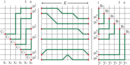
Figure 10: Nest of paths contributing to $\big{\langle}\Psi\big{(}{\bf v}_{[N\backslash n]}\big{)}\big{|}\bar{\sf F}_{n}^{+}{(-{{\sf H}})^{K}}\bar{\sf F}_{n}\big{|}\Psi({\bf u}_{N-n})\big{\rangle}$ at $N=6$, $n=2$ and $K=9$ (the gluing is along the wavy lines, where ${\widehat{\boldsymbol{\mu}}^{L,R}}$ are shown without the hats).

Equation which governs $G\big{(}{\widehat{\boldsymbol{\mu}}^{L}};{\widehat{\boldsymbol{\mu}}^{R}}|t\big{)}$ (7.19) is the same as (5.4), and its solution is given either by (5.6) or by (5.9),

$$G\big{(}{\widehat{\boldsymbol{\mu}}^{L}};{\widehat{\boldsymbol{\mu}}^{R}}\big{|}t\big{)}=\frac{{\rm e}^{tN}}{(M+1)^{N}}\sum\limits_{\{{\boldsymbol{\phi}}_{N}\}}{\rm e}^{-tE_{N}({\boldsymbol{\phi}}_{N})}\big{|}{\mathcal{V}}\big{(}{\rm e}^{{\rm i}{\boldsymbol{\phi}}_{N}}\big{)}\big{|}^{2}S_{{\widehat{\boldsymbol{\lambda}}}^{L}}\big{(}{\rm e}^{{\rm i}{\boldsymbol{\phi}}_{N}}\big{)}S_{{\widehat{\boldsymbol{\lambda}}^{R}}}\big{(}{\rm e}^{-{\rm i}{\boldsymbol{\phi}}_{N}}\big{)},$$ (7.22)

where ${\widehat{\boldsymbol{\lambda}}}^{L,R}=\widehat{\boldsymbol{\mu}}^{L,R}-{\boldsymbol{\delta}}_{N}$. The average (7.18) is re-expressed with regard at (7.22):

$$\big{\langle}\Psi\big{(}{\bf v}_{[N\backslash n]}\big{)}\big{|}\bar{\sf F}_{n}^{+}{\rm e}^{-\frac{t}{2}{{\sf H}}}\bar{\sf F}_{n}\big{|}\Psi({\bf u}_{N-n})\big{\rangle}={} \Bigg{(}\prod\limits_{l=1}^{N-n}\frac{u^{2n}_{l}}{v^{2n}_{l+n}}\Bigg{)}\frac{{\rm e}^{tN}}{(M+1)^{N}}\sum\limits_{\{{\boldsymbol{\phi}}_{N}\}}{\rm e}^{-tE_{N}({\boldsymbol{\phi}}_{N})}\big{|}{\mathcal{V}}\big{(}{\rm e}^{{\rm i}{\boldsymbol{\phi}}_{N}}\big{)}\big{|}^{2}$$

$$\times{\cal P}_{\cal M}\big{(}{\bf v}_{[N\backslash n]}^{-2},{\rm e}^{{\rm i}{\boldsymbol{\phi}}_{N}}\big{)}{\cal P}_{\cal M}\big{(}{\rm e}^{-{\rm i}{\boldsymbol{\phi}}_{N}},{\textbf{u}}_{N-n}^{2}\big{)},$$ (7.23)

where ${\cal P}_{\cal M}\big{(}{\bf v}_{[N\backslash n]}^{-2},{\rm e}^{{\rm i}{\boldsymbol{\phi}}_{N}}\big{)}$ and ${\cal P}_{\cal M}\big{(}{\rm e}^{-{\rm i}{\boldsymbol{\phi}}_{N}},{\textbf{u}}_{N-n}^{2}\big{)}$ are the generators of watermelons with deviation $n$ parameterized by the numbers of steps according to (3.30) and (3.31). This representation is useful in studying the asymptotical behaviour of (7.17).

Eventually, the representations (4.12), (5.2), and (7.23) allow us to express the persistence of domain wall (4.16) (or (7.17)) parameterized by (4.15):

$${\cal F}\big{(}{{\boldsymbol{\theta}}}_{[N\backslash n]}^{\rm g},n,t\big{)}={} \frac{\big{|}\mathcal{V}\big{(}{\rm e}^{{\rm i}{{\boldsymbol{\theta}}}_{[N\backslash n]}^{g}}\big{)}\big{|}^{2}}{(M+1)^{2N}}\sum\limits_{\{{\boldsymbol{\phi}}_{N}\}}{\rm e}^{-tE_{N}({\boldsymbol{\phi}}_{N})}$$

$$\times\big{|}{\mathcal{V}}({\rm e}^{{\rm i}{\boldsymbol{\phi}}_{N}})\big{|}^{2}{\cal P}_{\cal M}\big{(}{\rm e}^{-i{{\boldsymbol{\theta}}}_{[N\backslash n]}^{\rm g}},{\rm e}^{{\rm i}{\boldsymbol{\phi}}_{N}}\big{)}{\cal P}_{\cal M}\big{(}{\rm e}^{-{\rm i}{\boldsymbol{\phi}}_{N}},{\rm e}^{{\rm i}{{\boldsymbol{\theta}}}_{[N\backslash n]}^{\rm g}}\big{)}.$$ (7.24)

7.3 Auto-correlation function

Let us turn to the auto-correlation function (4.14). Analogously to (7.18), we obtain the average under off-shell parametrization:

$$\big{\langle}\Psi\big{(}{\bf v}_{[N\backslash n]}\big{)}\big{|}\bar{\sf F}_{n}^{+}{\rm e}^{-\frac{t_{1}}{2}{{\sf H}}}{\bar{\varPi}}_{m}{\rm e}^{-\frac{t_{2}}{2}{{\sf H}}}\bar{\sf F}_{n}\big{|}\Psi({\bf u}_{N-n})\big{\rangle}$$

$$\qquad{}=\Bigg{(}\prod\limits_{l=1}^{N-n}\frac{u^{2n}_{l}}{v^{2n}_{l+n}}\Bigg{)}\sum\limits_{{{\boldsymbol{\lambda}}^{L,R}}\subseteq\{{\mathcal{M}}^{N-n}\}}S_{{\widehat{{\boldsymbol{\lambda}}}^{L}}}\big{(}{\bf v}_{[N\backslash n]}^{-2}\big{)}S_{{\widehat{{\boldsymbol{\lambda}}}^{R}}}\big{(}{\textbf{u}}_{N-n}^{2}\big{)}G\big{(}{\widehat{{\boldsymbol{\mu}}}^{L}};{\widehat{{\boldsymbol{\mu}}}^{R}}\big{|}t_{1},t_{2},m\big{)},$$ (7.25)

where summation is similar to that in (7.18), and ${\textbf{u}}^{2}_{N-n}$, ${\textbf{v}}^{2}_{[N\backslash n]}$ stand for off-shell parametrization (see (2.10)). The generating function $G\big{(}{\widehat{{\boldsymbol{\mu}}}^{L}};{\widehat{{\boldsymbol{\mu}}}^{R}}\big{|}t_{1},t_{2},m\big{)}$ is given by (6.2):

$$G\big{(}{\widehat{{\boldsymbol{\mu}}}^{L}};{\widehat{{\boldsymbol{\mu}}}^{R}}\big{|}t_{1},t_{2},m\big{)}=\big{\langle}{\widehat{{\boldsymbol{\mu}}}^{L}}\big{|}{\rm e}^{-\frac{t_{1}}{2}{{\sf H}}}{\bar{\varPi}}_{m}{\rm e}^{-\frac{t_{2}}{2}{{\sf H}}}\big{|}{\widehat{{\boldsymbol{\mu}}}^{R}}\big{\rangle}.$$ (7.26)

Expanding (7.26) with respect of $\bigl{(}\frac{t_{1}}{2}\bigr{)}^{K_{1}}$ and $\bigl{(}\frac{t_{2}}{2}\bigr{)}^{K_{2}}$, we obtain a double series characterized by the coefficients (6.9) as follows:

$${\mathfrak{G}}\big{(}{\widehat{{\boldsymbol{\mu}}}^{L}};{\widehat{{\boldsymbol{\mu}}}^{R}}\big{|}K_{1},K_{2},m\big{)}=\big{\langle}{\widehat{{\boldsymbol{\mu}}}^{L}}\big{|}(-{{\sf H}})^{K_{1}}{\bar{\varPi}}_{m}(-{{\sf H}})^{K_{2}}\big{|}{\widehat{{\boldsymbol{\mu}}}^{R}}\big{\rangle}.$$ (7.27)

Equation (6.10), as well as its solution (6.11), are valid for the coefficients (7.27), which enumerate the nests of $(K_{1}+K_{2})$-step random turns walks connecting the sites ${\widehat{{\boldsymbol{\mu}}}^{L}}$ and ${\widehat{{\boldsymbol{\mu}}}^{R}}$. Equation (6.13) is also modified and takes the form:

$$\big{|}P_{K_{1}+K_{2}}\big{(}{\widehat{{\boldsymbol{\mu}}}^{L}}\underset{m}{\rightarrow}{\widehat{{\boldsymbol{\mu}}}^{R}}\big{)}\big{|} ={\mathfrak{G}}\big{(}{\widehat{{\boldsymbol{\mu}}}^{L}};{\widehat{{\boldsymbol{\mu}}}^{R}}\big{|}K_{1},K_{2},m\big{)}$$

$$=\sum_{\boldsymbol{\rho}\subseteq\{({\cal M}/m)^{N}\}}\big{|}P_{K_{1}}\big{(}{\widehat{{\boldsymbol{\mu}}}^{L}}\rightarrow{\boldsymbol{\rho}}+{{\boldsymbol{\delta}}}_{N}\big{)}\big{|}\big{|}P_{K_{2}}\big{(}{\boldsymbol{\rho}}+{{\boldsymbol{\delta}}}_{N}\rightarrow{\widehat{{\boldsymbol{\mu}}}^{R}}\big{)}\big{|}.$$ (7.28)

Equation (7.28) enumerates self-avoiding lattice paths of random turns vicious walkers going from ${\widehat{{\boldsymbol{\mu}}}^{L}}$ to ${\widehat{{\boldsymbol{\mu}}}^{R}}$ and infiltrating through a bottleneck: the projector forbids “visiting” the sites from $0^{\rm th}$ to $(m-1)^{\rm th}$. The correlation function (7.25) corresponds to summation over the nests with all possible $K_{1}$ and $K_{2}$ and over all ${{{\boldsymbol{\mu}}}^{L}}$ and ${{{\boldsymbol{\mu}}}^{R}}$.

The transition amplitude (7.25) admits a representation of the same type as (7.23), which includes the generating functions of watermelons ${\cal P}_{{\cal M}/m}$ (3.17) and the generating functions of watermelons with deviation ${\cal P}_{\cal M}$, (3.30) and (3.31). With regard at (6.2) and (7.25), (7.26), the auto-correlation function (4.14) takes the form:

$$\Gamma\big{(}{{\boldsymbol{\theta}}}_{[N\backslash n]}^{\rm g},N,n,m,t_{1},t_{2}\big{)}$$

$$\qquad{}=\frac{\big{|}\mathcal{V}\big{(}{\rm e}^{{\rm i}{{\boldsymbol{\theta}}}_{[N\backslash n]}^{g}}\big{)}\big{|}^{2}}{(M+1)^{N}}\sum\limits_{{{\boldsymbol{\lambda}}^{L,R}}\subseteq\{{\mathcal{M}}^{N-n}\}}S_{{\widehat{{\boldsymbol{\lambda}}}^{L}}}\big{(}{\rm e}^{-{\rm i}{{\boldsymbol{\theta}}}_{[N\backslash n]}^{g}}\big{)}S_{{\widehat{{\boldsymbol{\lambda}}}^{R}}}\big{(}{\rm e}^{{\rm i}{{\boldsymbol{\theta}}}_{[N\backslash n]}^{g}}\big{)}{\cal G}\big{(}{\widehat{{\boldsymbol{\mu}}}^{L}};{\widehat{{\boldsymbol{\mu}}}^{R}}\big{|}t_{1},t_{2},m\big{)},$$

or, equivalently,

$$\Gamma({{\boldsymbol{\theta}}}_{[N\backslash n]}^{\rm g},N,n,m,t_{1},t_{2})$$

$$\quad{}=\frac{|\mathcal{V}({\rm e}^{{\rm i}{{\boldsymbol{\theta}}}_{[N\backslash n]}^{g}})|^{2}}{(M+1)^{3N}}\!\sum\limits_{\{{\boldsymbol{\phi}}_{N}\}}\!\sum\limits_{\{{\boldsymbol{\phi}}^{\prime}_{N}\}}\!{\rm e}^{-t_{1}E_{N}({\boldsymbol{\phi}}^{\prime}_{N})-t_{2}E_{N}({\boldsymbol{\phi}}_{N})}\big{|}{\mathcal{V}}\big{(}{\rm e}^{{\rm i}{\boldsymbol{\phi}}_{N}}\big{)}\big{|}^{2}\big{|}{\mathcal{V}}\big{(}{\rm e}^{{\rm i}{\boldsymbol{\phi}}^{\prime}_{N}}\big{)}\big{|}^{2}{\cal P}_{\cal M}\big{(}{\rm e}^{-{\rm i}{{\boldsymbol{\theta}}}_{[N\backslash n]}^{g}},{\rm e}^{{\rm i}{\boldsymbol{\phi}}_{N}}\big{)}$$

$$\quad\hphantom{=\frac{|\mathcal{V}({\rm e}^{{\rm i}{{\boldsymbol{\theta}}}_{[N\backslash n]}^{g}})|^{2}}{(M+1)^{3N}}\!\sum\limits_{\{{\boldsymbol{\phi}}_{N}\}}\!\sum\limits_{\{{\boldsymbol{\phi}}^{\prime}_{N}\}}\!}{}\times{\cal P}_{{\cal M}/m}\big{(}{\rm e}^{-{\rm i}{\boldsymbol{\phi}}_{N}},{\rm e}^{{\rm i}{\boldsymbol{\phi}}^{\prime}_{N}}\big{)}{\cal P}_{\cal M}\big{(}{\rm e}^{-{\rm i}{\boldsymbol{\phi}}^{\prime}_{N}},{\rm e}^{{\rm i}{{\boldsymbol{\theta}}}_{[N\backslash n]}^{g}}\big{)}.$$ (7.29)

The representation (7.29) is reduced at $m=0$ to (7.24).

8 Asymptotics of dynamical correlation functions

The representations (7.24) and (7.29) are related with the corresponding generating functions of watermelons given by equations (3.22), (3.23) (Proposition 3.8) and (3.35), (3.36) (Proposition 3.11). In turn, the asymptotics of these representations are related with the numbers of plane partitions (7.5) in ${\cal B}(N,N,{\mathcal{M}}-m)$ and the numbers of plane partitions (7.16) in ${\cal B}(N-n,N,{\mathcal{M}})$.

Indeed, let us obtain the leading estimates for the correlation functions at large evolution parameter $t\gg 1$ in the case of long enough chain, $M\gg 1$, and moderate $N$, $1\ll N\ll M$ (double scaling limit). The discrete parameters of summation in (7.24) and (7.29), the same as in (5.9), fill at large enough $M$ the segment $[-\pi,\pi]\ni\phi$. The corresponding summations are replaced approximately by multiple integration, and the matrix integrals arise for (7.24) and (7.29). The leading approximation for the integrals is provided by steepest descent [12] due to $\cos\phi\simeq 1$ at $t\gg 1$.

Firstly, the transition amplitude (5.1) given by (5.2) and by the integral expressing (7.22) behaves at $t\gg 1$ in leading approximation:

$${\cal G}\big{(}\widehat{{\boldsymbol{\mu}}}^{L};\widehat{{\boldsymbol{\mu}}}^{R}\big{|}t\big{)}\simeq S_{\widehat{{\boldsymbol{\lambda}}}^{L}}({\textbf{1}})S_{{\widehat{{\boldsymbol{\lambda}}}^{R}}}({\textbf{1}})\frac{{\cal I}_{N}}{t^{{N^{2}}/{2}}},$$ (8.1)

where $S_{\widehat{{\boldsymbol{\lambda}}}^{L,R}}({\textbf{1}})$ are given by (3.2), and ${\cal I}_{N}$ is a special form of Mehta’s integral connected with the partition function of Gaussian unitary ensemble [33]:

$$\displaystyle{{\cal I}_{N}\equiv\frac{1}{N!}\int\limits_{-\infty}^{\infty}\!\int\limits_{-\infty}^{\infty}\cdots\int\limits_{-\infty}^{\infty}{\rm e}^{-\frac{1}{2}\sum\limits_{l=1}^{N}x^{2}_{l}}\!\!\prod_{1\leq k<l\leq N}\bigl{|}x_{k}-x_{l}\bigr{|}^{2}\prod_{k=1}^{N}\frac{{\rm d}x_{k}}{2\pi}}=\prod_{l=0}^{N-1}\frac{l!}{(2\pi)^{1/2}}.$$ (8.2)

Provided that right-hand side of (8.2) is expressed through the Barnes $G$-function [1], the following estimate arises [3]:

$$\log{\cal I}_{N}=\frac{N^{2}}{2}\log N-\frac{3N^{2}}{4}+{\cal O}(\log N),\qquad N\gg 1.$$ (8.3)

Analogously to (8.1), the persistence of domain wall ${\cal F}\big{(}{{\boldsymbol{\theta}}}_{[N\backslash n]}^{\rm g},n,t\big{)}$ (7.24) behaves at $t\gg 1$:

$${\cal F}\big{(}{{\boldsymbol{\theta}}}_{[N\backslash n]}^{\rm g},n,t\big{)}\simeq\frac{\mathcal{A}(N,n)}{t^{{N^{2}}/{2}}},$$ (8.4)

$${\mathcal{A}}(N,n)\equiv A^{2}(N-n,N,M-N+1)\bigg{(}\frac{2\pi}{M+1}\bigg{)}^{N^{2}}{\cal I}_{N}^{3},$$ (8.5)

where the estimate

$$\frac{1}{{\mathcal{N}}^{2}\big{(}{{\boldsymbol{\theta}}}^{\rm g}_{[N\backslash n]}\big{)}}\simeq\frac{(2\pi)^{(N-n)(N-n-1)}}{(M+1)^{(N-n)^{2}}}\prod_{1\leq r<s\leq N-n}|r-s|^{2}\underset{N\gg n}{\approx}\bigg{(}\frac{2\pi}{M+1}\bigg{)}^{N^{2}}{\cal I}_{N}^{2}$$

is taken into account [4].

The coefficient ${\mathcal{A}}(N,n)$ (8.5) includes $A^{2}(N-n,N,M-N+1)$, where

$$A(N-n,N,M-N+1)=\lim_{q\to 1}W_{q}(N-n,N,{\mathcal{M}}),$$ (8.6)

and $W_{q}(N-n,N,{\mathcal{M}})$ is the generating function of watermelons with deviation (3.35) or (3.36). Equivalently, $A(N-n,N,M-N+1)$ is the number of plane partitions (3.50) in a box ${\mathcal{B}}(N-n,N,M-N+1)$ of the height $M-N+1$ and $(N-n)\times N$ bottom.

The asymptotics (8.1) of the transition amplitude (5.1) and the asymptotics (8.4) of the domain wall persistence (4.16) demonstrate the power law decay governed by the same critical exponent $N^{2}/2$, however different combinatorial factors characterize the amplitudes.

Combining (6.2), (6.7) and (7.22), we estimate the transition amplitude ${\cal G}\big{(}{\widehat{{\boldsymbol{\mu}}}^{L}};{\widehat{{\boldsymbol{\mu}}}^{R}}\big{|}t_{1},t_{2},m\big{)}$ (see also (6.1)):

$${\cal G}\big{(}{\widehat{{\boldsymbol{\mu}}}^{L}};{\widehat{{\boldsymbol{\mu}}}^{R}}\big{|}t_{1},t_{2},m\big{)}\simeq S_{\widehat{{\boldsymbol{\lambda}}}^{L}}({\textbf{1}})S_{\widehat{{\boldsymbol{\lambda}}}^{R}}({\textbf{1}})A(N,N,M-m-N+1)\frac{{\cal I}^{2}_{N}}{(t_{1}t_{2})^{{N^{2}}/{2}}}.$$ (8.7)

The coefficient $A(N,N,M-m-N+1)$ is given:

$$A(N,N,M-m-N+1)=\lim_{q\to 1}W_{q}(N,{\mathcal{M}}/m),$$

where $W_{q}(N,{\mathcal{M}}/m)$ is the generating function of the watermelons without deviation (3.22) or (3.23). Equivalently, $A(N,N,M-m-N+1)$ is the number (2.38) of plane partitions in the box $\mathcal{B}(N,N,M-m-N+1)$ of the height $M-m-N+1$ with square $N\times N$ bottom.

Eventually, the representation (7.29) allows us to estimate the auto-correlation function (4.14) when $1\ll N\ll M$ and $t_{1},t_{2}\gg 1$:

$$\Gamma\big{(}{{\boldsymbol{\theta}}}_{[N\backslash n]}^{\rm g},N,n,m,t_{1},t_{2}\big{)}\simeq\frac{\mathcal{A}(N,n,m)}{(t_{1}t_{2})^{{N^{2}}/{2}}},$$ (8.8)

$${\mathcal{A}}(N,n,m)\equiv A(N,N,M-m-N+1)A^{2}(N-n,N,M-N+1)\bigg{(}\frac{2\pi}{M+1}\bigg{)}^{N^{2}}{\cal I}_{N}^{4}.$$ (8.9)

The critical exponent is the same in (8.7) and (8.8), whereas the combinatorial amplitudes are different.

The representation of the generating function $W_{q}(N-n,N,{\mathcal{M}})$ of the watermelons with deviation is due to Theorem 3.13 provided that $\delta=n$ and $M\to\infty$. Therefore it is appropriate to use (3.51) in the limiting formula (8.6) for studying (8.4) or (8.8) for the chain of infinite length. Equation (3.51), as the norm-trace generating function, enables enumeration of the plane partitions with fixed traces of diagonal entries [5].

We have shown that both asymptotics, (8.4) or (8.8), are related with enumeration of the random walks of the lock step type. The asymptotical behavior of the combinatorial contributions $A(N,N,M-m-N+1)$ and $A(N-n,N,M-N+1)$ in the double scaling limit is provided by [4]. Together with (8.3), the limiting behavior of (8.4) and (8.8) is completely described in the double scaling limit.

9 Conclusion

In this paper we have dealt with the calculation of the auto-correlation functions of the $XX0$ Heisenberg spin chain. We have presented the exact expressions of the correlation functions in terms of different types of nests of self-avoiding lattice walks, namely in terms of lock steps and random turns walks. In particular, the representation of the persistence of domain wall correlation function admits a visualization in terms of the lattice paths infiltrating through a bottleneck. Such a description is an essential result of our study. The asymptotical estimates in the double scaling limit at large value of the evolution parameter demonstrate that the correlation functions in question are multiples of the numbers of the watermelons or, equivalently, of the numbers of the plane partitions distributed in a high box.

Acknowledgments

This work was supported by the Russian Science Foundation (Grant 18-11-00297). We are grateful to the referees for their comments and suggestions which enabled to improve the paper.

References

- [1] Barnes E.W., The theory of the -function, Quart. J. Math. 31 (1900), 264–314.
- [2] Bogoliubov N.M., Heisenberg chain and random walks, J. Math. Sci. 138 (2006), 5636–5643.
- [3] Bogoliubov N.M., Malyshev C., Correlation functions of Heisenberg chain, -binomial determinants, and random walks, Nuclear Phys. B 879 (2014), 268–291, arXiv:1401.7624.
- [4] Bogoliubov N.M., Malyshev C., Integrable models and combinatorics, Russian Math. Surveys 70 (2015), 789–856.
- [5] Bogoliubov N.M., Malyshev C., The phase model and the norm-trace generating function of plane partitions, J. Stat. Mech. Theory Exp. 2018 (2018), 083101, 13 pages.
- [6] Bogoliubov N.M., Malyshev C., Heisenberg chain and random walks on a ring, Zap. Nauchn. Sem. POMI 494 (2020), 48–63.
- [7] Borodin A., Gorin V., Rains E.M., -distributions on boxed plane partitions, Selecta Math. (N.S.) 16 (2010), 731–789, arXiv:0905.0679.
- [8] Bressoud D.M., Proofs and confirmations. The story of the alternating sign matrix conjecture, MAA Spectrum, Cambridge University Press, Cambridge, 1999.
- [9] Bufetov A., Gorin V., Fluctuations of particle systems determined by Schur generating functions, Adv. Math. 338 (2018), 702–781, arXiv:1604.01110.
- [10] Carlitz L., Some determinants of -binomial coefficients, J. Reine Angew. Math. 226 (1967), 216–220.
- [11] Colomo F., Izergin A.G., Korepin V.E., Tognetti V., Correlators in the Heisenberg chain as Fredholm determinants, Phys. Lett. A 169 (1992), 243–247.
- [12] Dingle R.B., Asymptotic expansions: their derivation and interpretation, Academic Press, London – New York, 1973.
- [13] Faddeev L.D., Quantum completely integrable models in field theory, in Mathematical Physics Reviews, Vol. 1, Soviet Sci. Rev. Sect. C: Math. Phys. Rev., Vol. 1, Harwood Academic, Chur, 1980, 107–155.
- [14] Faddeev L.D., Takhtadzhyan L.A., Spectrum and scattering of excitations in the one-dimensional isotropic Heisenberg model, J. Sov. Math. 24 (1984), 241–267.
- [15] Faddeev L.D., Takhtajan L.A., What is the spin of a spin wave?, Phys. Lett. A 85 (1981), 375–377.
- [16] Fisher M.E., Walks, walls, wetting, and melting, J. Stat. Phys. 34 (1984), 667–729.
- [17] Forrester P.J., Exact solution of the lock step model of vicious walkers, J. Phys. A: Math. Gen. 23 (1990), 1259–1273.
- [18] Forrester P.J., Exact results for vicious walker models of domain walls, J. Phys. A: Math. Gen. 24 (1991), 203–218.
- [19] Franchini F., Its A.R., Korepin V.E., Takhtajan L.A., Spectrum of the density matrix of a large block of spins of the model in one dimension, Quantum Inf. Process. 10 (2011), 325–341.
- [20] Fulton W., Young tableaux. With applications to representation theory and geometry, London Mathematical Society Student Texts, Vol. 35, Cambridge University Press, Cambridge, 1997.
- [21] Gessel I., Viennot G., Binomial determinants, paths, and hook length formulae, Adv. Math. 58 (1985), 300–321.
- [22] Gross D.J., Witten E., Possible third-order phase transition in the large- lattice gauge theory, Phys. Rev. D 21 (1980), 446–453.
- [23] Guttmann A.J., Owczarek A.L., Viennot X.G., Vicious walkers and Young tableaux. I. Without walls, J. Phys. A: Math. Gen. 31 (1998), 8123–8135.
- [24] Karlin S., McGregor J., Coincidence probabilities, Pacific J. Math. 9 (1959), 1141–1164.
- [25] Karlin S., McGregor J., Coincidence properties of birth and death processes, Pacific J. Math. 9 (1959), 1109–1140.
- [26] Katori M., Tanemura H., Nonintersecting paths, noncolliding diffusion processes and representation theory, RIMS Kōkyūroku 1438 (2005), 83–102, arXiv:math.PR/0501218.
- [27] Katori M., Tanemura H., Noncolliding Brownian motion and determinantal processes, J. Stat. Phys. 129 (2007), 1233–1277, arXiv:0705.2460.
- [28] Klimyk A., Schmüdgen K., Quantum groups and their representations, Texts and Monographs in Physics, Springer-Verlag, Berlin, 1997.
- [29] Krattenthaler C., Guttmann A.J., Viennot X.G., Vicious walkers, friendly walkers and Young tableaux. II. With a wall, J. Phys. A: Math. Gen. 33 (2000), 8835–8866, arXiv:cond-mat/0006367.
- [30] Lieb E., Schultz T., Mattis D., Two soluble models of an antiferromagnetic chain, Ann. Physics 16 (1961), 407–466.
- [31] Lindström B., On the vector representations of induced matroids, Bull. London Math. Soc. 5 (1973), 85–90.
- [32] Macdonald I.G., Symmetric functions and Hall polynomials, 2nd ed., Oxford Mathematical Monographs, The Clarendon Press, Oxford University Press, New York, 1995.
- [33] Mehta M.L., Random matrices, 2nd ed., Academic Press, Inc., Boston, MA, 1991.
- [34] Okounkov A., Reshetikhin N., Correlation function of Schur process with application to local geometry of a random 3-dimensional Young diagram, J. Amer. Math. Soc. 16 (2003), 581–603, arXiv:math.CO/0107056.
- [35] Pérez-García D., Tierz M., Mapping between the Heisenberg spin chain and low-energy QCD, Phys. Rev. X 4 (2014), 021050, 12 pages.
- [36] Saeedian M., Zahabi A., Phase structure of spin chain and nonintersecting Brownian motion, J. Stat. Mech. Theory Exp. 2018 (2018), 013104, 36 pages, arXiv:1612.03463.
- [37] Saeedian M., Zahabi A., Exact solvability and asymptotic aspects of generalized spin chains, Phys. A 549 (2020), 124406, 19 pages, arXiv:1709.02760.
- [38] Santilli L., Tierz M., Phase transition in complex-time Loschmidt echo of short and long range spin chain, J. Stat. Mech. Theory Exp. 2020 (2020), 063102, 39 pages, arXiv:1902.06649.
- [39] Sklyanin E.K., Takhtajan L.A., Faddeev L.D., Quantum inverse problem method. I, Theoret. and Math. Phys. 40 (1979), 688–706.
- [40] Stanley R.P., Enumerative combinatorics, Vol. 1, Cambridge Studies in Advanced Mathematics, Vol. 49, Cambridge University Press, Cambridge, 1997.
- [41] Stanley R.P., Enumerative combinatorics, Vol. 2, Cambridge Studies in Advanced Mathematics, Vol. 62, Cambridge University Press, Cambridge, 1999.
- [42] Stembridge J.R., Multiplicity-free products of Schur functions, Ann. Comb. 5 (2001), 113–121.
- [43] Takhtajan L.A., The picture of low-lying excitations in the isotropic Heisenberg chain of arbitrary spins, Phys. Lett. A 87 (1982), 479–482.
- [44] Takhtajan L.A., Faddeev L.D., The quantum method for the inverse problem and the Heisenberg model, Russian Math. Surveys 34 (1979), no. 5, 11–68.
- [45] van Willigenburg S., Equality of Schur and skew Schur functions, Ann. Comb. 9 (2005), 355–362, arXiv:math.CO/0410044.
- [46] Vershik A.M., Statistical mechanics of combinatorial partitions, and their limit shapes, Funct. Anal. Appl. 30 (1996), 90–105.