Abstract

We quantitatively estimate the effect of the UV physics on the Casimir energy in a five-dimensional (5D) model on $S^{1}/Z_{2}$. If the cutoff scale of the 5D theory is not far from the compactification scale, the UV physics may affect the low energy result. We work in the cutoff regularization scheme by introducing two independent cutoff scales for the spatial momentum in the non-compact space and for the Kaluza-Klein masses. The effects of the UV physics are incorporated as a damping effect of the contributions to the vacuum energy around the cutoff scales. We numerically calculate the Casimir energy and evaluate the deviation from the result obtained in the zeta-function regularization, which does not include information on the UV physics. We find that the result well agrees with the latter for the Gaussian-type damping, while it can deviate for the kink-type one.

1 Introduction

The Casimir effect is a well-known macroscopic quantum effect [1]. It has been observed by various experiments, and the observed values well agree with the theoretical predictions [2]-[5]. The Casimir effect can also play an important role in the context of the extra dimensions. It generates the scalar potential for the volume modulus of the compact extra space, and can stabilize the modulus to a finite value [6]-[11].

The Casimir energy is defined as the energy difference between the vacuum state in the presence of the conducting plates and that in the absence of the plates. Since the vacuum energies in quantum theories generically diverge, we have to regularize them before taking the difference. There are various ways to calculate the Casimir energy with different regularization schemes, and the same results are obtained in the renormalizable theories by those methods [12]-[18]. However, it is also known that there can be a mismatch between the results obtained using different regularizations in some cases [19]-[23]. Such discrepancies come from the (regularized) divergent part of the vacuum energies. Among various regularizations, the cutoff regularization is presumably the most physically intuitive way to regularize the divergent quantities. Ref. [22] clarified the conditions that the Casimir energy becomes the cutoff independent, and is finite. It also pointed out that the zeta-function regularization discard the cutoff dependence that may have some physical information on the UV physics. For the four-dimensional (4D) electrodynamics, the fact that the experimental values are in agreement with the theoretical predictions indicates that such cutoff dependences are negligible. However, this does not ensure that they can always be negligible in any theories.

The superstring theory is a promising candidate of the final theory that contains the quantum gravity, and predicts the existence of the extra space dimensions. Such extra space is often supposed to be compactified on some manifolds or orbifolds in order to explain the fact that the observed space dimension is three. So if we detect any signal that suggests the extra dimensions, it strongly supports the superstring theory. The existence of the compact extra space affects the time evolution of the universe because it modifies the Einstein equation. Therefore, the search for the deviation from the standard cosmological evolution is useful to test the superstring theory. The current cosmological obervations indicate that the spacetime evolves the Freedman equation that oiginates from the 4D Einstein equation. Thus the size of the compact space should be stabilized at a small finite value, so that its effects on the cosmological evolution of the universe are suppressed at late times. In our previous work [24], we investigated the time evolution of the domain-wall configuration in the $S^{1}$ extra dimension, which can be regarded as the 3-brane we live. In that setup, the extra dimension continues to expand due to the repulsive force between the kinks. Hence we need some moduli-stabilization mechanism in order to obtain the (approximate) 4D FLRW universe at late times. As we mentioned, the Casimir effect can be used for such stabilization. In fact, if the Casimir force is attractive, it can balance with the repulsive force between the kinks.

Since the extra-dimensional models are non-renormalizable, it should be regarded as effective theories of more fundamental theories. In other words, they have UV cutoff scales. In this paper, we discuss a five-dimensional (5D) scalar theory compactified on $S^{1}/Z_{2}$ as a simple example. The theory behaves as a 5D theory between the cutoff scale $\Lambda$ and the compactification scale $1/R$, where $R$ is the radius of $S^{1}$. In particular, when the cutoff $\Lambda$ is not far from $1/R$, effects of the UV physics might give non-negligible contributions to the result. Such effects will appear as a cutoff-dependence of the Casimir energy.

The purpose of this work is to quantitatively estimate the UV-cutoff dependence of the Casimir energy, and to clarify the situation in which it is non-negligible. For our purpose, we work in the cutoff regularization scheme, do not take the limit $\Lambda\to\infty$, and numerically evaluate the deviation from the result obtained by the conventional methods, which corresponds to the limit of $\Lambda\to\infty$.

The paper is organized as follows. In the next section, we provide a brief review of the conventional calculations for the Casimir energy. In Sec. 3, we introduce the cutoff scales for the momentum and the Kaluza-Klein masses, and derive the expression of the Casimir energy. In Sec. 4, we numerically calculate the Casimir energy, and evaluate the deviation from the conventional result. Sec. 5 is devoted to the summary and discussions. In the appendices, we collect some formulae used in our calculations.

2 Conventional calculations for Casimir energy

In this section, we provide a brief review of the conventional way to calculate the Casimir energy [2]-[9]. To simplify the discussion, we consider a real scalar theory in the flat $D$-dimensional spacetime, and one of the spatial dimensions is compactified on $S^{1}/Z_{2}$.

$${\cal L}\!\!\! =\!\!\! -\frac{1}{2}\partial^{\mu}\Phi\partial_{\mu}\Phi-\frac{1}{2}M^{2}\Phi^{2},$$ (2.1)

where $\mu=0,1,\cdots,D-1$, $M$ is the bulk mass parameter. The coordinate of the compact dimension is denoted as $y$. The fundamental region of $S^{1}/Z_{2}$ is chosen as $0\leq y\leq\pi R$, where $R$ is the radius of $S^{1}$. The real scalar field $\Phi$ is assumed to be $Z_{2}$ odd. Thus, it satisfies the Dirichlet boundary conditions at the boundaries of $S^{1}/Z_{2}$, in addition to the periodic boundary condition. As a result of these boundary conditions, the Kaluza-Klein (KK) masses are determined by

$$\sin\left(\pi R\sqrt{m_{n}^{2}-M^{2}}\right)=0,$$ (2.2)

whose solutions are

$$m_{n}=\sqrt{M^{2}+\frac{n^{2}}{R^{2}}}.\;\;\;\;\;\left(n=1,2,\cdots\right)$$ (2.3)

Then, the vacuum energy density in the $(D-1)$-dimensional effective theory is expressed as

$$E_{\rm vac}=\sum_{n=1}^{\infty}\int\frac{d^{d}k}{2(2\pi)^{d}}\;\omega_{n}(k),$$ (2.4)

where $d\equiv D-2$ is the dimension of the non-compact space, and

$$\omega_{n}(k)\equiv\sqrt{k^{2}+m_{n}^{2}}\;\;\;\;\;\left(k^{2}\equiv|\vec{k}|^{2}\right)$$ (2.5)

is the energy of a KK mode with the $d$-dimensional momentum $\vec{k}$ and the mass $m_{n}$.

To perform the $\vec{k}$-integral, we work in the dimensional regularization, and obtain

$$E_{\rm vac}\!\!\! =\!\!\! -\frac{\Gamma(-\frac{d+1}{2})}{2(4\pi)^{(d+1)/2}}\sum_{n=1}^{\infty}m_{n}^{d+1},$$ (2.6)

where $\Gamma(\alpha)$ is the Euler gamma function. The infinite sum over the KK modes is evaluated by means of the zeta function regularization technique [8, 15, 16]. Using the formula (B.19), the above expression becomes

$$E_{\rm vac}\!\!\! =\!\!\! -\frac{\Gamma(-\frac{d+1}{2})}{2(4\pi)^{(d+1)/2}R^{d+1}}\left\{-\frac{\bar{M}^{d+1}}{2}+\frac{\sqrt{\pi}\Gamma(-\frac{d+2}{2})}{2\Gamma(-\frac{d+1}{2})}\bar{M}^{d+2}\right.$$ (2.7)

$$\hskip 99.58464pt\left.+\frac{2\bar{M}^{\frac{d+2}{2}}}{\pi^{\frac{d+1}{2}}\Gamma(-\frac{d+1}{2})}\sum_{n=1}^{\infty}n^{-\frac{d+2}{2}}K_{\frac{d+2}{2}}\left(2\pi n\bar{M}\right)\right\}$$

$$=\!\!\! \frac{\Gamma(-\frac{d+1}{2})M^{d+1}}{4(4\pi)^{(d+1)/2}}-\frac{\Gamma(-\frac{d+2}{2})}{8(4\pi)^{d/2}}RM^{d+2}$$

$$-\frac{M^{\frac{d+2}{2}}}{(2\pi)^{d+1}R^{d/2}}\sum_{n=1}^{\infty}n^{-\frac{d+2}{2}}K_{\frac{d+2}{2}}\left(2\pi nMR\right),$$

where $\bar{M}\equiv MR$. The first term is irrelevant to the Casimir force because it is independent of $R$. The second term gives a constant Casimir force, which is also present even in the case of $R\to\infty$. Since the physically relevant Casimir force is the difference between the above $E_{\rm vac}$ and that of the non-compact case (i.e., $R\to\infty$), the contribution from the second term in (2.7) is cancelled. Thus, the Casimir energy $E_{\rm cas}$ is given by

$$E_{\rm cas}=-\frac{M^{\frac{d+2}{2}}}{(2\pi)^{d+1}R^{d/2}}\sum_{n=1}^{\infty}n^{-\frac{d+2}{2}}K_{\frac{d+2}{2}}\left(2\pi nMR\right).$$ (2.8)

In the massless case ($M=0$), (2.8) reduces to

$$E_{\rm cas}^{(M=0)}\!\!\! =\!\!\! -\frac{1}{2^{d+1}\pi^{\frac{3}{2}d+2}R^{d+1}}\sum_{n=1}^{\infty}\frac{1}{n^{d+2}}\lim_{M\to 0}\left(\pi nMR\right)^{\frac{d+2}{2}}K_{\frac{d+2}{2}}\left(2\pi nMR\right)$$ (2.9)

$$=\!\!\! -\frac{1}{2^{d+1}\pi^{\frac{3}{2}d+2}R^{d+1}}\sum_{n=1}^{\infty}\frac{1}{n^{d+2}}\frac{\Gamma(\frac{d+2}{2})}{2}$$

$$=\!\!\! -\frac{\Gamma(\frac{d+2}{2})\zeta(d+2)}{2^{d+2}\pi^{\frac{3}{2}d+2}R^{d+1}},$$

where $\zeta(s)$ is the Riemann zeta function. We have used the formula:

$$\lim_{z\to 0}z^{\alpha}K_{\alpha}(2z)=\frac{\Gamma(\alpha)}{2}.\;\;\;\;\;\left(\alpha>0\right)$$ (2.10)

Namely, we have

$$E_{\rm cas}^{(M=0)}=\begin{cases}\displaystyle-\frac{\zeta(3)}{16\pi^{3}R^{2}}&\left(d=1\right)\\ \displaystyle\rule{0.0pt}{24.0pt}-\frac{1}{1440\pi R^{3}}&\left(d=2\right)\\ \displaystyle\rule{0.0pt}{24.0pt}-\frac{3\zeta(5)}{128\pi^{6}R^{4}}&\left(d=3\right)\\ \displaystyle\rule{0.0pt}{24.0pt}-\frac{1}{30240\pi^{2}R^{5}}&\left(d=4\right)\end{cases}.$$ (2.11)

The Casimir energy (2.8) can be also expressed in the following integral form by using the formula (B.12).

$$E_{\rm cas}\!\!\! =\!\!\! -\frac{\Gamma(-\frac{d+1}{2})}{2(4\pi)^{(d+1)/2}R^{d+1}}\cdot\frac{d+1}{\pi}\sin\frac{(d+1)\pi}{2}\int_{0}^{\infty}dw\;w^{d}\ln\left(1-e^{-2\pi\sqrt{w^{2}+\bar{M}^{2}}}\right)$$ (2.12)

$$=\!\!\! \frac{1}{(4\pi)^{(d+1)/2}\Gamma(\frac{d+1}{2})R^{d+1}}\int_{0}^{\infty}dw\;w^{d}\ln\left(1-e^{-2\pi\sqrt{w^{2}+\bar{M}^{2}}}\right).$$

We have used the reflection formula for the gamma function in the second line.

The bulk mass $M$ exponentially suppresses the Casimir Energy as shown in Fig. 1.

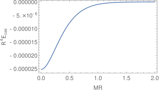
Figure 1: $R^{4}E_{\rm cas}$ in the case of $D=5$ as a function of $MR$.

3 Cutoff regularization

Since the expression (2.4) diverges, we need some physical condition that extracts a finite physically-sensible contribution, i.e., the Casimir energy (density) $E_{\rm cas}$, from the divergent quantity $E_{\rm vac}$. To see this extraction explicitly, the dimensional regularization and the zeta function regularization are not suitable. Thus we work in the cutoff regularization. We introduce the momentum cutoff $\Lambda$ and the cutoff for the KK masses $\tilde{\Lambda}$, independently. In contrast to the conventional calculations, we keep them finite.

As a condition to extract the finite energy density, we define the Casimir energy $E_{\rm cas}$ in such a way that it vanishes when the size of the compactification radius is taken to infinite. Namely, the energy density (in the $D$-dimensional spacetime) is measured from that in the non-compact limit [26]. In this work, we discuss the global Casimir energy, for simplicity. Thus, this condition is adopted to the averaged energy density over the compact space $E_{\rm vac}/\pi R$. Therefore, the Casimir energy $E_{\rm cas}$, which is defined as the vacuum energy density in the $(D-1)$-dimensional effective theory, is defined as

$$\frac{E_{\rm cas}(R)}{\pi R}\equiv\frac{E_{\rm vac}(R)}{\pi R}-\lim_{R\to\infty}\frac{E_{\rm vac}(R)}{\pi R}.$$ (3.1)

3.1 Momentum cutoff

First, we perform the $\vec{k}$-integral.

$$\int\frac{d^{d}k}{2(2\pi)^{d}}\;\left(k^{2}+m_{n}^{2}\right)^{1/2}\!\!\! =\!\!\! \frac{2\pi^{d/2}}{\Gamma(\frac{d}{2})}\int_{0}^{\Lambda}\frac{dk}{2(2\pi)^{d}}\;k^{d-1}\left(k^{2}+m_{n}^{2}\right)^{1/2}$$ (3.2)

$$=\!\!\! \frac{m_{n}^{d+1}}{2(4\pi)^{d/2}\Gamma(\frac{d}{2})}\int_{\epsilon_{n}}^{1}ds\;s^{-\frac{d+1}{2}-1}\left(1-s\right)^{\frac{d}{2}-1}$$

$$=\!\!\! \frac{m_{n}^{d+1}}{2(4\pi)^{d/2}\Gamma(\frac{d}{2})}\beta_{\epsilon_{n}}\left(-\frac{d+1}{2},\frac{d}{2}\right),$$

where $\Lambda$ is the $d$-dimensional momentum cutoff scale, $2\pi^{d/2}/\Gamma(\frac{d}{2})$ is the area of the $(d-1)$-dimensional sphere with a unit radius,

$$s\equiv\frac{m_{n}^{2}}{k^{2}+m_{n}^{2}},\;\;\;\;\;\epsilon_{n}\equiv\frac{m_{n}^{2}}{\Lambda^{2}+m_{n}^{2}},$$ (3.3)

and $\beta_{z}(\alpha,\beta)$ is the incomplete beta function defined in (A.3). Thus, (2.4) is expressed as

$$E_{\rm vac}\!\!\! =\!\!\! \frac{1}{2(4\pi)^{d/2}\Gamma(\frac{d}{2})}\lim_{N\to\infty}\sum_{n=1}^{N}m_{n}^{d+1}\beta_{\epsilon_{n}}\left(-\frac{d+1}{2},\frac{d}{2}\right).$$ (3.4)

The explicit forms of $\beta_{\epsilon_{n}}$ in (3.4) for various values of $d$ are collected in Appendix A.2.

If we take the limit $\Lambda\to\infty$ before taking the limit $N\to\infty$, the above expression reduces to (2.6) in the previous section since 

$$\lim_{\epsilon_{n}\to 0}\beta_{\epsilon_{n}}\left(-\frac{d+1}{2},\frac{d}{2}\right)=B\left(-\frac{d+1}{2},\frac{d}{2}\right)=\frac{\Gamma(-\frac{d+1}{2})\Gamma(\frac{d}{2})}{\Gamma(-\frac{1}{2})}.$$ (3.5)

This indicates that, in the derivation of the Casimir energy shown in the previous section, we have implicitly assumed that the contributions from the KK modes near the cutoff $m_{n}\sim\Lambda$ are negligibly small. In the next section, we will numerically check whether this is true or not.

3.2 Cutoff for KK masses

Here we introduce the cutoff scale $\tilde{\Lambda}$ for the KK masses. Naively, the regularized vacuum energy is written as

$$E_{\rm vac}=\frac{1}{2(4\pi)^{d/2}\Gamma(\frac{d}{2})}\sum_{n=1}^{N}m_{n}^{d+1}\beta_{\epsilon_{n}}\left(-\frac{d+1}{2},\frac{d}{2}\right),$$ (3.6)

where

$$N\equiv{\rm floor}\,\left(R\sqrt{\tilde{\Lambda}^{2}-M^{2}}\right)$$ (3.7)

is the cutoff for the number of the KK modes. However, it seems natural to assume that the contributions of the KK modes near the cutoff are suppressed by the UV physics. So we introduce the damping function that has the property:

$$g_{N}(x)\simeq\begin{cases}1&\mbox{for $x\ll N$}\\ 0&\mbox{for $x\gg N$}\end{cases},$$ (3.8)

and consider the following quantity instead of (3.6).

$$E_{\rm vac}\!\!\! =\!\!\! \frac{1}{2(4\pi)^{d/2}\Gamma(\frac{d}{2})}\sum_{n=1}^{\infty}m_{n}^{d+1}\beta_{\epsilon_{n}}\left(-\frac{d+1}{2},\frac{d}{2}\right)g_{N}(n).$$ (3.9)

As examples of the damping function, we can take

$$g_{N}(x)=\exp\left(-\frac{x^{2}}{2N^{2}}\right),$$ (3.10)

or

$$g_{N}(x)=\frac{1}{2}\left[1+\tanh\left\{A\left(1-\frac{x}{N}\right)\right\}\right],$$ (3.11)

where $A$ is a positive constant that controls the steepness around the cutoff (see Fig. 2).

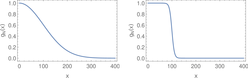
Figure 2: The profiles of the damping function $g_{N}(x)$ for (3.10) (left plot) and for (3.11) (right plot). The cutoff $N$ and the constant $A$ are chosen as $10^{2}$ and $10$, respectively.

We cannot choose too small values of $A$. Otherwise the damping effect reaches around $x=0$, and the property (3.8) is no longer satisfied. As we will see in the next section, $A\gtrsim 10$ is required.

We rewrite (3.9) in terms of the dimensionless constants:

$$a\equiv\frac{1}{\Lambda R},\;\;\;\;\;\hat{M}\equiv\frac{M}{\Lambda},$$ (3.12)

as

$$E_{\rm vac}=\frac{\Lambda^{d+1}}{2(4\pi)^{d/2}\Gamma(\frac{d}{2})}\sum_{n=1}^{\infty}F(an),$$ (3.13)

where

$$F(x)\!\!\! \equiv\!\!\! f(X(x))g_{N}(x),$$

$$X(x)\!\!\! \equiv\!\!\! \sqrt{\hat{M}^{2}+x^{2}},$$

$$f(X)\!\!\! \equiv\!\!\! \beta_{\frac{X^{2}}{1+X^{2}}}\left(-\frac{d+1}{2},\frac{d}{2}\right)X^{d+1}.$$ (3.14)

From (A.8)-(A.11), the explicit forms of the function $f(X)$ are given by

$$f(X)=\begin{cases}\displaystyle\sqrt{1+X^{2}}+X^{2}\ln\frac{1+\sqrt{1+X^{2}}}{X}&D=3\;\;(d=1)\\ \displaystyle\rule{0.0pt}{23.0pt}\frac{2}{3}\left\{\left(1+X^{2}\right)^{\frac{3}{2}}-X^{3}\right\}&D=4\;\;(d=2)\\ \displaystyle\rule{0.0pt}{27.0pt}\frac{1}{4}\left\{\left(2+X^{2}\right)\sqrt{1+X^{2}}-X^{4}\ln\frac{1+\sqrt{1+X^{2}}}{X}\right\}&D=5\;\;(d=3)\\ \displaystyle\rule{0.0pt}{23.0pt}\frac{2}{15}\left\{\left(3-2X^{2}\right)\left(1+X^{2}\right)^{\frac{3}{2}}+2X^{5}\right\}&D=6\;\;(d=4)\end{cases}.$$ (3.15)

Although the explicit functional forms of $f(X)$ for different values of $D$ are quite different, they have a similar behavior. In fact, we find that

$$f(0)=\frac{2}{D-1},$$ (3.16)

and

$$f(X)\sim\frac{2}{D-2}X.\;\;\;\left(\mbox{for $X\gg 1$}\right)$$ (3.17)

Fig. 3 shows the profile of $f(X)$ in each dimension.

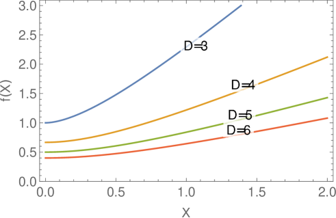
Figure 3: The profiles of the function $f(X)$ in (3.15) for various dimensions.

Due to the damping function $g_{N}(x)$, the function $F(x)$ satisfies the boundary conditions,

$$\lim_{x\to\infty}F(x)=0,\;\;\;\;\;\lim_{x\to\infty}F^{(p)}(x)=0.\;\;\;(p=1,2,3,\cdots)$$ (3.18)

3.3 Non-compact limit

Next consider the non-compact limit ($R\to\infty$) in order to evaluate the Casimir energy given in (3.1). When we take this limit, we have to treat the contribution of the zero-mode carefully because it is projected out by the orbifold boundary conditions. Let us first consider the case of the $S^{1}$ compactification instead of $S^{1}/Z_{2}$. Then, the sum in (3.13) is taken over the whole integers. In this case, we can easily take the non-compact limit.

$$\lim_{R\to\infty}\frac{E^{S^{1}}_{\rm vac}(R)}{\pi R}\!\!\! =\!\!\! \frac{\Lambda^{d+2}}{2\pi(4\pi)^{d/2}\Gamma(\frac{d}{2})}\lim_{a\to 0}\sum_{n=-\infty}^{\infty}aF(an)$$ (3.19)

$$=\!\!\! \frac{\Lambda^{d+2}}{2\pi(4\pi)^{d/2}\Gamma(\frac{d}{2})}\int_{-\infty}^{\infty}dx\;F(x).$$

Thus, we have

$$\frac{E_{\rm cas}^{S^{1}}}{\pi R}\!\!\! =\!\!\! \frac{E^{S^{1}}_{\rm vac}(R)}{\pi R}-\lim_{R\to\infty}\frac{E^{S^{1}}_{\rm vac}(R)}{\pi R}$$ (3.20)

$$=\!\!\! \frac{\Lambda^{d+2}}{2\pi(4\pi)^{d/2}\Gamma(\frac{d}{2})}\left\{\sum_{n=-\infty}^{\infty}aF(an)-\int_{-\infty}^{\infty}dx\;F(x)\right\}$$

$$=\!\!\! \frac{\Lambda^{d+2}a}{2\pi(4\pi)^{d/2}\Gamma(\frac{d}{2})}\left\{\sum_{n=-\infty}^{\infty}F(an)-\int_{-\infty}^{\infty}dx\;F(ax)\right\}.$$

We have used that

$$\frac{1}{a}\int_{-\infty}^{\infty}dx\;F(x)=\int_{-\infty}^{\infty}dx\;F(ax).$$ (3.21)

Since $F(x)$ is an even function, the brace part in (3.20) can be rewritten as

$$\sum_{n=-\infty}^{\infty}F(an)-\int_{-\infty}^{\infty}dx\;F(ax)=2\sum_{n=1}^{\infty}F(an)+F(0)-2\int_{0}^{\infty}dx\;F(ax).$$ (3.22)

Now let us come back to the case of $S^{1}/Z_{2}$. Noting that (3.20) is finite in the limit of $\Lambda\to\infty$, we should identify the non-compact limit of the energy density as 

$$\lim_{R\to\infty}\frac{E_{\rm vac}(R)}{\pi R}=\frac{\Lambda^{d+2}}{2\pi(4\pi)^{d/2}\Gamma(\frac{d}{2})}\left\{\int_{0}^{\infty}dx\;F(x)-\frac{1}{2}F(0)\right\}.$$ (3.24)

Thus the Casimir energy in this case is expressed as

$$E_{\rm cas}\!\!\! =\!\!\! \frac{\Lambda^{d+1}}{2(4\pi)^{d/2}\Gamma(\frac{d}{2})}\Delta(a)=\frac{\Delta(a)/a^{d+1}}{2(4\pi)^{d/2}\Gamma(\frac{d}{2})R^{d+1}},$$ (3.25)

where

$$\Delta(a)\equiv\sum_{n=1}^{\infty}F(an)-\int_{0}^{\infty}dx\;F(ax)+\frac{1}{2}F(0).$$ (3.26)

4 Calculation of Casimir energy

In this section, we numerically calculate the Casimir energy in the cutoff regularization scheme, and evaluate the deviation from the conventional result. As mentioned in Sec. 3.2, the behaviors of $f(X)$ in (3.15) are similar for different $D$. Thus the qualitative features of the Casimir energy do not depend on $D$ very much. Therefore we focus on the case of $D=5$ ($d=3$) in this section.

4.1 Expression of Casimir energy

In (3.12), we have normalized the bulk mass $M$ by the cutoff scale $\Lambda$. Since $\hat{M}$ is independent of $R$, it can be treated as a constant when we take the non-compact limit ($R\to\infty$). However, once we obtain the expression (3.25) with (3.26), it is more convenient to normalize $M$ by the compactification scale $1/R$ rather than the cutoff scale $\Lambda$. Hence we define

$$\bar{M}\equiv RM,$$ (4.1)

and rewrite $\Delta(a)$ defined in (3.26) as

$$\Delta(a)=\sum_{n=1}^{\infty}\bar{F}(n)-\int_{0}^{\infty}dx\;\bar{F}(x)+\frac{1}{2}\bar{F}(0),$$ (4.2)

where

$$\bar{F}(x)\!\!\! \equiv\!\!\! f(a\bar{X}(x))g_{N}(x)$$

$$\bar{X}(x)\!\!\! \equiv\!\!\! \sqrt{\bar{M}^{2}+x^{2}}.$$ (4.3)

In order to evaluate $\Delta(a)$ in (4.2), the Euler-Maclaurin formula is useful (see Appendix C.1) [12, 25, 27]. Using the formula (C.1), $\Delta(a)$ is expressed as

$$\Delta(a)\!\!\! =\!\!\! \lim_{n_{\rm max}\to\infty}\left\{\sum_{n=1}^{n_{\rm max}}\bar{F}(n)-\int_{0}^{n_{\rm max}}dx\;\bar{F}(x)+\frac{1}{2}\bar{F}(0)\right\}$$ (4.4)

$$=\!\!\! \lim_{n_{\rm max}\to\infty}\left\{\sum_{n=0}^{n_{\rm max}}\bar{F}(n)-\int_{0}^{n_{\rm max}}dx\;\bar{F}(x)\right\}-\frac{1}{2}\bar{F}(0)$$

$$=\!\!\! \lim_{n_{\rm max}\to\infty}\left[\frac{1}{2}\left\{\bar{F}(0)+\bar{F}(n_{\rm max})\right\}+\sum_{p=1}^{\lfloor q/2\rfloor}\frac{B_{2p}}{(2p)!}\left\{\bar{F}^{(2p-1)}(n_{\rm max})-\bar{F}^{(2p-1)}(0)\right\}+R_{q}\right]$$

$$-\frac{1}{2}\bar{F}(0)$$

$$=\!\!\! -\sum_{p=1}^{\lfloor q/2\rfloor}\frac{B_{2p}}{(2p)!}\bar{F}^{(2p-1)}(0)+R_{q},$$

where $B_{2q}$ are the Bernoulli numbers (see (C.2)). We have used the condition (3.18) at the last equality. The remainder term $R_{q}$ is defined as

$$R_{q}\equiv(-1)^{q-1}\int_{0}^{\infty}dx\;\frac{B_{q}(x-\lfloor x\rfloor)}{q!}\bar{F}^{(q)}(x),$$ (4.5)

where $B_{q}(x)$ is the Bernoulli polynomial (see (C.4)), and the symbol $\lfloor\cdots\rfloor$ denotes the floor function. The integer $q$ can be chosen to an arbitrary value greater than 1. Here we set it as $q=2$. Then, (4.4) becomes

$$\Delta(a)=-\frac{1}{12}\bar{F}^{(1)}(0)+R_{2},$$ (4.6)

and the remainder term is expressed as

$$R_{2}\!\!\! =\!\!\! -\int_{0}^{\infty}dx\;\frac{B_{2}(x-\lfloor x\rfloor)}{2}\bar{F}^{(2)}(x)$$ (4.7)

$$=\!\!\! -\frac{1}{2}\sum_{k=0}^{\infty}\int_{k}^{k+1}dx\;B_{2}(x-k)\bar{F}^{(2)}(x).$$

Due to the property (3.8), we have $g_{N}(0)\simeq 1$, and thus the first term in (4.6) vanishes because

$$\bar{F}^{(1)}(0)\simeq\left\{\partial_{x}f(a\bar{X}(x))\right\}_{x=0}=\left\{\frac{ax}{\bar{X}(x)}f^{(1)}(a\bar{X}(x))\right\}_{x=0}=0.$$ (4.8)

4.2 Case of Gaussian damping

Here we choose the Gaussian-type damping function (3.10). In order to see the deviation from the conventional result, we define the ratio:

$$r_{E}\equiv\frac{E_{\rm cas}}{E_{\rm cas}^{\rm conv}},$$ (4.9)

where $E_{\rm cas}^{\rm conv}$ is the Casimir energy calculated in the conventional methods, such as (2.8) or (2.12). Fig. 4 shows the ratio $r_{E}$ as a function of the bulk mass $\bar{M}=MR$. In this plot, we have chosen the cutoff scales as $\tilde{\Lambda}=\Lambda$.

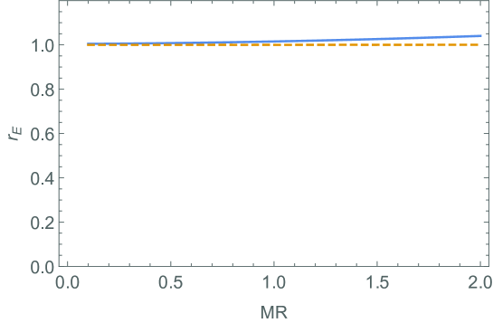
Figure 4: The ratio (4.9) as a function of the bulk mass $\bar{M}=MR$. The blue solid and orange dashed lines represent the case of $\Lambda R=\tilde{\Lambda}R=10$ and $100$, respectively.

As this plot shows, the deviation is small and can be neglected if $\Lambda R$ is larger than $10^{2}$. Therefore, the cutoff-dependence of $E_{\rm cas}$ is negligible, and the conventional result is reliable even in the case of a finite cutoff scale $\Lambda$ unless $\Lambda R={\cal O}(10)$. This is true also in the case of $\tilde{\Lambda}\neq\Lambda$ as long as they are in the same order of magnitude.

4.3 Case of kink-like damping

4.3.1 General properties

Next we consider the case of the kink-type damping function (3.11). Fig. 5 shows the ratio $r_{E}$ as a function of the parameter $A$ in the damping function. The cutoff scale are chosen as $\Lambda R=100$, and $\tilde{\Lambda}=\Lambda$ (blue solid), $2\Lambda$ (orange dashed) and $0.5\Lambda$ (green dotted). The bulk mass is chosen as $\bar{M}=MR=0.1$.

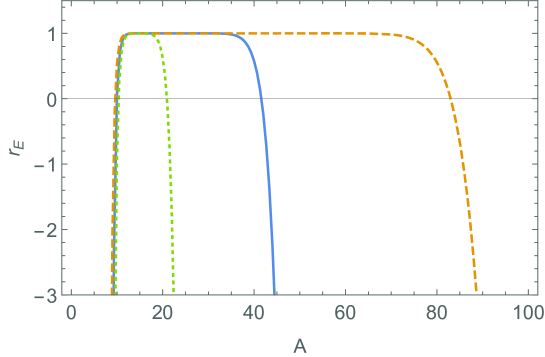
Figure 5: The ratio (4.9) as a function of $A$ in the damping function (3.11). The cutoff scale is chosen as $a=10^{-2}$, and the bulk mass is chosen as $\bar{M}=0.1$. The blue solid, the orange dashed and the green dotted lines represent the case of $\tilde{\Lambda}=\Lambda$, $2\Lambda$ and $0.5\Lambda$, respectively.

For $A\lesssim 10$, the ratio $r_{E}$ deviates from one because the damping effect reaches near the origin and the property (3.8) is no longer satisfied. Namely, $g_{N}(x)$ is not suitable for the damping function when $A\lesssim 10$. In the case of $\tilde{\Lambda}=\Lambda$, the result agrees with the conventional one for $10\lesssim A\lesssim 35$. However, for $A\gtrsim 35$, the ratio $r_{E}$ starts to deviate from one, flips the sign and becomes negatively larger and larger. We can also see that the upper limit of the region in which the result agrees with the conventional one is sensitive to the ratio of the cutoffs $\tilde{\Lambda}/\Lambda$.

4.3.2 The limit of $A\to\infty$

In order to understand the behavior of $r_{E}$ for large values of $A$, we consider the limit of $A\to\infty$. Since

$$\bar{F}^{(2)}(x)\!\!\! =\!\!\! \partial_{x}^{2}\left\{{\cal F}(x)g_{N}(x)\right\}$$ (4.10)

$$=\!\!\! {\cal F}^{(2)}(x)g_{N}(x)+2{\cal F}^{(1)}(x)g_{N}^{(1)}(x)+{\cal F}(x)g_{N}^{(2)}(x),$$

where ${\cal F}(x)\equiv f(a\bar{X}(x))$, and $g_{N}^{(1)}(x)$ and $g_{N}^{(2)}(x)$ sharply localizes around $x=N$ when $A$ is large, (4.7) is rewritten as

$$R_{2}\!\!\! =\!\!\! -\frac{1}{2}\sum_{k=0}^{\infty}\int_{k}^{k+1}dx\;B_{2}(x-k){\cal F}^{(2)}(x)g_{N}(x)$$ (4.11)

$$-\frac{1}{2}\sum_{k=N-1}^{N}\int_{k}^{k+1}dx\;B_{2}(x-k)\left\{2{\cal F}^{(1)}(x)g_{N}^{(1)}(x)+{\cal F}(x)g_{N}^{(2)}(x)\right\}.$$

In the limit of $A\to\infty$, the damping function $g_{N}(x)$ and its derivatives become

$$g_{N}(x)\!\!\! \to\!\!\! \Theta(N-x),$$

$$g_{N}^{(1)}(x)\!\!\! \to\!\!\! -\delta(x-N),$$

$$g_{N}^{(2)}(x)\!\!\! \to\!\!\! -\delta^{(1)}(x-N),$$ (4.12)

where $\Theta(x)$ is the Heaviside step function. Therefore, we have

$$\sum_{k=N-1}^{N}\int_{k}^{k+1}dx\;B_{2}(x-k){\cal F}^{(1)}(x)g_{N}^{(1)}(x)$$ (4.13)

$$=\!\!\! \int_{N-1}^{N}dx\;B_{2}(x-N+1){\cal F}^{(1)}(x)g_{N}^{(1)}(x)+\int_{N}^{N+1}dx\;B_{2}(x-N){\cal F}^{(1)}(x)g_{N}^{(1)}(x)$$

$$\to\!\!\! -\frac{1}{2}B_{2}(1){\cal F}^{(1)}(N)-\frac{1}{2}B_{2}(0){\cal F}^{(1)}(N)=-\frac{1}{6}{\cal F}^{(1)}(N),$$

and

$$\sum_{k=N-1}^{N}\int_{k}^{k+1}dx\;B_{2}(x-k){\cal F}(x)g_{N}^{(2)}(x)$$ (4.14)

$$=\!\!\! \sum_{N-1}^{N}\left\{\left[B_{2}(x-k){\cal F}(x)g_{N}^{(1)}(x)\right]_{k}^{k+1}-\int_{k}^{k+1}dx\;\partial_{x}\left\{B_{2}(x-k){\cal F}(x)\right\}g_{N}^{(1)}(x)\right\}$$

$$=\!\!\! B_{2}\left\{{\cal F}(N+1)g_{N}^{(1)}(N+1)-{\cal F}(N-1)g_{N}^{(1)}(N-1)\right\}$$

$$-\sum_{N-1}^{N}\int_{k}^{k+1}dx\;\left\{2B_{1}(x-k){\cal F}(x)+B_{2}(x-k){\cal F}^{(1)}(x)\right\}g_{N}^{(1)}(x)$$

$$\to\!\!\! \frac{1}{2}\left\{2B_{1}(1){\cal F}(N)+B_{2}(1){\cal F}(N)\right\}+\frac{1}{2}\left\{2B_{1}(0){\cal F}^{(1)}(N)+B_{2}(0){\cal F}^{(1)}(N)\right\}$$

$$=\!\!\! B_{2}{\cal F}^{(1)}(N)=\frac{1}{6}{\cal F}^{(1)}(N).$$

We have used that

$$\lim_{A\to\infty}\int_{N-1}^{N}dx\;{\cal G}(x)g_{N}^{(1)}(x)\!\!\! =\!\!\! -\frac{1}{2}{\cal G}(N),$$

$$\lim_{A\to\infty}\int_{N}^{N+1}dx\;{\cal G}(x)g_{N}^{(1)}(x)\!\!\! =\!\!\! -\frac{1}{2}{\cal G}(N),$$ (4.15)

for an arbitrary function ${\cal G}(x)$, and

$$\partial_{x}B_{2}(x)\!\!\! =\!\!\! 2B_{1}(x),\;\;\;\;\;\lim_{A\to\infty}g_{N}^{(1)}(N\pm 1)=0,$$

$$B_{1}(0)\!\!\! =\!\!\! -B_{1}(1)=-\frac{1}{2},$$

$$B_{2}(0)\!\!\! =\!\!\! B_{2}(1)=B_{2}=\frac{1}{6}.$$ (4.16)

Therefore, since

$$\bar{F}^{(1)}(0)={\cal F}^{(1)}(0)=\left\{a\bar{X}^{(1)}(x)f^{(1)}(a\bar{X}(x))\right\}_{x=0}=\left\{\frac{ax}{\bar{X}(x)}f^{(1)}(a\bar{X}(x))\right\}_{x=0}=0,$$ (4.17)

(4.6) is expressed as

$$\Delta(a)\!\!\! =\!\!\! R_{2}=-\frac{1}{2}\sum_{k=0}^{N-1}\int_{k}^{k+1}dx\;B_{2}(x-k){\cal F}^{(2)}(x)+\frac{1}{6}{\cal F}^{(1)}(N)-\frac{1}{2}\left\{\frac{1}{6}{\cal F}^{(1)}(N)\right\}$$ (4.18)

$$=\!\!\! -\frac{1}{2}\sum_{k=0}^{N-1}\int_{0}^{1}dx\;B_{2}(x){\cal F}^{(2)}(x+k)+\frac{1}{12}{\cal F}^{(1)}(N).$$

In the $D=5$ case, we have

$${\cal F}^{(1)}(N)\!\!\! =\!\!\! a^{2}N\left\{\sqrt{1+a^{2}(\bar{M}^{2}+N^{2})}-a^{2}\left(\bar{M}^{2}+N^{2}\right)\ln\frac{1+\sqrt{1+a^{2}(\bar{M}^{2}+N^{2})}}{a\sqrt{\bar{M}^{2}+N^{2}}}\right\},$$

$${\cal F}^{(2)}(x)\!\!\! =\!\!\! \frac{a^{2}}{\sqrt{1+a^{2}(\bar{M}^{2}+x^{2})}}\bigg{[}1$$

$$\hskip 28.45274pt+a^{2}\left(\bar{M}^{2}+3x^{2}\right)\left\{1-\sqrt{1+a^{2}(\bar{M}^{2}+x^{2})}\ln\frac{1+\sqrt{1+a^{2}(\bar{M}^{2}+x^{2})}}{a\sqrt{\bar{M}^{2}+x^{2}}}\right\}\bigg{]}.$$

Fig. 6 shows the Casimir energy $E_{\rm cas}$ as a function of $\ln(\Lambda R)$. From this plot, we can see that $E_{\rm cas}$ grows as ${\cal O}(10^{-5}\Lambda R)$ for $\Lambda R>10^{3}$.

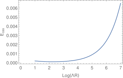
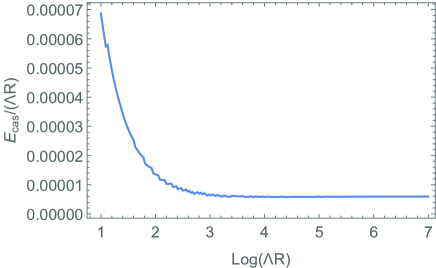
Figure 6: The Casimir energy $E_{\rm cas}$ and $E_{\rm cas}/(\Lambda R)$ in the limit of $A\to\infty$ as functions of $\ln(\Lambda R)$.

Namely, the Casimir energy calculated by using the sharp kink damping function diverges as $\Lambda\to\infty$. We should also notice that the Casimir energy in this limit $\lim_{A\to\infty}E_{\rm cas}$ is positive, which has the opposite sign to the conventional result.

4.3.3 Cutoff dependence

As we mentioned in Sec. 3.1, the deviation from the conventional result comes from the contributions of the KK modes near the cutoff scale $m_{n}\sim\Lambda$. The Casimir energy $E_{\rm cas}$ is expressed as

$$E_{\rm cas}=\frac{1}{8\pi^{2}R^{4}}\frac{\Delta(a)}{a^{4}},$$ (4.20)

where

$$\Delta(a)\!\!\! =\!\!\! \sum_{n=1}^{\infty}\bar{F}(n)-\int_{0}^{\infty}dx\;\bar{F}(x)+\frac{1}{2}\bar{F}(0).$$ (4.21)

Fig. 7 shows the profile of $\bar{F}(x)$ in the case of the Gaussian and the kink-like damping functions (the kink-parameter $A$ is chosen as 10, 30 and 50).

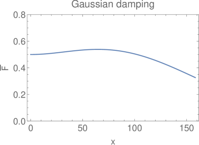
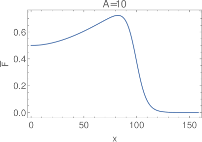
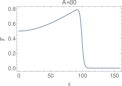
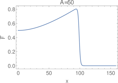
Figure 7: The profile of $\bar{F}(x)$ in (4.3) in the case of the Gaussian damping function (top left), $A=10$ (top right), $A=30$ (bottom left) and $A=50$ (bottom right). The bulk mass and the cutoff scale are chosen as $\bar{M}=MR=0.1$ and $\Lambda R=100$, respectively.

From these figures, we can see that the contributions from the modes near the cutoff scale $m_{n}\sim\Lambda$ are well suppressed in the case of the Gaussian damping (3.10). Thus the result almost agrees with the conventional one (2.8) or (2.12). In contrast, the kink-like damping function (3.11) takes account of those contributions with only small suppression. If the kink shape is not very steep, the deviation from the conventional result still remains tiny. However, if the damping function becomes close to the step function, the deviation becomes large and $E_{\rm cas}$ changes the sign as discussed in Sec. 4.3.2.

The range of $A$ in which the conventional result is reproduced depends on the hierarchy between the cutoff scale and the compactification scale $1/R$. The plots in Fig. 8 show the ratio $r_{E}$ in the cases of $a=3\times 10^{-2}$ (the left plot) and of $a=3\times 10^{-3}$ (the right plot). We can see that the conventional result is reproduced in a wider range of $A$ for larger cutoff scales. When the cutoff is not high enough, we cannot obtain the conventional result for any values of $A$.

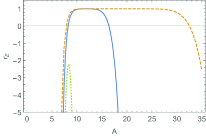
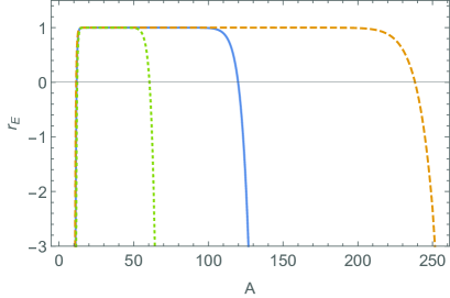
Figure 8: The ratio (4.9) as a function of $A$ in the damping function (3.11). The cutoff scale is chosen as $a=(\Lambda R)^{-1}=3\times 10^{-2}$ (left plot) and $a=3\times 10^{-3}$ (right plot). The bulk mass is chosen as $\bar{M}=0.1$. The blue solid, the orange dashed and the green dotted lines represent the case of $\tilde{\Lambda}=\Lambda$, $2\Lambda$ and $0.5\Lambda$, respectively.

5 Summary and discussions

We have numerically estimate the UV cutoff dependence of the global Casimir energy in a simple scalar model whose one spatial dimension is compactified on $S^{1}/Z_{2}$. We keep the cutoff scales finite, and evaluate the deviation from the conventional result obtained in the zeta-function regularization, which implicitly discards the UV physics information. This deviation originates from the contribution of the KK modes near the cutoff scale $m_{n}\sim\Lambda$. We can easily show that the sharp cutoff for the KK masses leads to a large deviation, which changes the sign of the Casimir energy. When $\Lambda R>10^{3}$, this energy is of ${\cal O}(10^{-5}\Lambda R)$. Instead of adopting such a sharp cutoff, we introduce a damping function and insert it into the infinite KK summation. We consider two types of the damping function. One is the Gaussian-type and the other is the kink-type. In the former case, the contributions near the cutoff scale are well suppressed, and the result almost agrees with the conventional one. In the latter case, the calculations take into account the modes near the cutoff, but the deviation from the conventional result still remains tiny unless the kink is extremely steep. When the hierarchy between the compactification scale $1/R$ and the cutoff scales $\Lambda$, $\tilde{\Lambda}$ is large, the conventional result is reproduced for a wide range of the kink parameter $A$ defined in (3.11). However, if the hierarchy is not large enough, such a region becomes narrow and the contributions from the KK modes near the cutoff tend to give a non-negligible contribution to the Casimir energy.

Since the 5D extra-dimensional model is non-renormalizable and should be regarded as an effective theory, it is expected that the contribution of the KK modes to the vacuum energy becomes suppressed as the KK mass approaches to the cutoff scale of the 5D theory due to the effect of the UV physics. Our result indicates that the Casimir energy can receive sizable contribution from the modes near the cutoff scale, depending on how much the contribution to the vacuum energy is damped near the cutoff. In particular, such a deviation from the conventional result tends to appear when the cutoff scale is not far from the compactification scale.

The damping function $g_{N}(x)$ introduced in this work mimics the suppression of the contributions from higher KK modes by the UV physics. For example, let us consider a spontaneously broken supersymmetric (SUSY) model. The low-energy effective theory is non-SUSY, and a nonvanishing vacuum energy is induced by the non-SUSY field content. Above the SUSY-breaking scale $\Lambda_{\rm SB}$, however, the superpartners start to contribute to the vacuum energy, and their contributions have opposite signs. Therefore, the total contributions from the modes above $\Lambda_{\rm SB}$ are partly cancelled. In the non-SUSY effective theory, the cancellation by the superpartners is represented by the damping function $g_{N}(x)$ inserted into the KK summation for the vacuum energy. It is interesting to investigate this damping effect in specific models that have UV-completed theories. For example, we can calculate the Casimir energy in a 6D theory with two extra dimensions compactified on a torus. If there is a hierarchy between the two radii of the torus, an effective 5D theory appears at intermediate scales. Then we can explicitly see how the contribution to the vacuum energy from each KK mode behaves near the cuoff of the effective 5D theory, and evaluate the deviation from the conventional Casimir energy.

We have worked in the flat spacetime. Although the KK mass spectrum depends on the geometry of the extra space, the level spacing for the KK masses becomes almost the same in the UV region, i.e., $\Delta m_{n}\equiv m_{n+1}-m_{n}\sim 1/R$. Hence the contribution from the KK modes around the cutoff does not depend the geometry very much. Our result is common in various 5D models. However, if the extra space has more dimensions, the distributions of the KK mass eigenvalues around the cutoff scale are quite different from that of 5D theories. Therefore, it is also interesting to extend our work to higher extra dimensions.

In this work, we have adopted the sharp cutoff for the momentum $\vec{k}$, for simplicity. To investigate the contributions of the modes near the cutoff in more detail, we should also introduce the damping function for the momentum integral. But we expect that the qualitative features obtained in this work do not change very much.

We have calculated the one-loop contribution to the Casimir energy in this paper. This is enough because we considered the free theory. However, once the interaction terms are included, higher-loop contributions will appear [28, 29, 30]. In such a case, some divergent terms are induced on the orbifold fixed points [29], and thus the corresponding brane terms are need to be introduced in order to renormalize them. We can construct a model in which the higher-loop contributions are subdominant if the cutoff-independence of the Casimir energy is ensured [30]. In the case that the cutoff-dependence cannot be neglected, it does not obvious whether the cutoff-dependence at two-loop is smaller than that of one-loop. We need to check this point when we include the interactions.

We will discuss these issues in separate papers.

Appendix A Incomplete beta and gamma functions

A.1 Definitions and properties

The integral expressions of the complete beta and the gamma functions are given by

$$B(\alpha,\beta)\!\!\! \equiv\!\!\! \int_{0}^{\infty}dx\;x^{\alpha-1}(1-x)^{\beta-1}=B(\beta,\alpha),$$

$$\Gamma(\alpha)\!\!\! \equiv\!\!\! \int_{0}^{\infty}dt\;t^{\alpha-1}e^{-t}.$$ (A.1)

These expressions are valid only for ${\rm Re}\,\alpha>0$ and ${\rm Re}\,\beta>0$. They are related as

$$B(\alpha,\beta)=\frac{\Gamma(\alpha)\Gamma(\beta)}{\Gamma(\alpha+\beta)}.$$ (A.2)

This relation holds over the whole domain of the beta function.

The incomplete beta functions are defined as

$$B_{z}(\alpha,\beta)\!\!\! \equiv\!\!\! \int_{0}^{z}dx\;x^{\alpha-1}(1-x)^{\beta-1},$$

$$\beta_{z}(\alpha,\beta)\!\!\! \equiv\!\!\! B(\alpha,\beta)-B_{z}(\alpha,\beta)=\int_{z}^{1}dx\;x^{\alpha-1}\left(1-x\right)^{\beta-1},$$ (A.3)

and the upper and the lower incomplete gamma functions are defined as

$$\Gamma_{z}(\alpha)\!\!\! \equiv\!\!\! \int_{z}^{\infty}dt\;t^{\alpha-1}e^{-t},$$

$$\gamma_{z}(\alpha)\!\!\! \equiv\!\!\! \Gamma(\alpha)-\Gamma_{z}(\alpha)=\int_{0}^{z}dt\;t^{\alpha-1}e^{-t}.$$ (A.4)

For $\alpha+\beta+1>0$ and $\beta>0$, it follows that

$$\beta_{\epsilon}(\alpha,\beta)=\frac{1}{\beta\Gamma(\alpha+\beta)}\int_{0}^{\infty}d\tau\;\tau^{\beta}e^{-\tau}\Gamma_{\tau\epsilon/(1-\epsilon)}(\alpha)+\frac{1}{\beta}\epsilon^{\alpha}(1-\epsilon)^{\beta}.$$ (A.5)

This reduces to (A.2) in the limit of $\epsilon\to 0$ if $\alpha>0$.

A.2 Explicit forms of Incomplete beta functions

The explicit forms of $\beta_{\epsilon_{n}}(-\frac{d+1}{2},\frac{d}{2})$, where $\epsilon_{n}\equiv m_{n}^{2}/(\Lambda^{2}+m_{n}^{2})$, are obtained as follows. Since

$$\partial_{\Lambda}\beta_{\epsilon_{n}}\left(\alpha,\beta\right)\!\!\! =\!\!\! -\epsilon_{n}^{\alpha-1}\left(1-\epsilon_{n}\right)^{\beta-1}\partial_{\Lambda}\epsilon_{n}$$ (A.6)

$$=\!\!\! \left(\frac{m_{n}^{2}}{\Lambda^{2}+m_{n}^{2}}\right)^{\alpha-1}\left(\frac{\Lambda^{2}}{\Lambda^{2}+m_{n}^{2}}\right)^{\beta-1}\frac{2\Lambda m_{n}^{2}}{\left(\Lambda^{2}+m_{n}^{2}\right)^{2}}$$

$$=\!\!\! \frac{2\Lambda^{2\beta-1}m_{n}^{2\alpha}}{\left(\Lambda^{2}+m_{n}^{2}\right)^{\alpha+\beta}},$$

and $\beta_{\epsilon_{n}}(\alpha,\beta)|_{\Lambda=0}=0$, we have

$$\beta_{\epsilon_{n}}\left(-\frac{d+1}{2},\frac{d}{2}\right)=\int_{0}^{\Lambda}d\Lambda^{\prime}\;\partial_{\Lambda^{\prime}}\beta_{\epsilon_{n}}\left(-\frac{d+1}{2},\frac{d}{2}\right)=\int_{0}^{\Lambda}d\Lambda^{\prime}\;\frac{2\Lambda^{\prime d-1}m_{n}^{-d-1}}{\left(\Lambda^{\prime 2}+m_{n}^{2}\right)^{-\frac{1}{2}}}.$$ (A.7)

Performing the integral, we obtain

$D=3\;(d=1)$

$$\beta_{\epsilon_{n}}\left(-1,\frac{1}{2}\right)\!\!\! =\!\!\! \frac{\Lambda\sqrt{\Lambda^{2}+m_{n}^{2}}}{m_{n}^{2}}+\ln\frac{\Lambda+\sqrt{\Lambda^{2}+m_{n}^{2}}}{m_{n}},$$ (A.8)

$D=4\;(d=2)$

$$\beta_{\epsilon_{n}}\left(-\frac{3}{2},1\right)\!\!\! =\!\!\! \frac{2\left(\Lambda^{2}+m_{n}^{2}\right)^{\frac{3}{2}}}{3m_{n}^{3}}-\frac{2}{3}.$$ (A.9)

$D=5\;(d=3)$

$$\beta_{\epsilon_{n}}\left(-2,\frac{3}{2}\right)\!\!\! =\!\!\! \frac{\Lambda}{4m_{n}^{4}}\left(2\Lambda^{2}+m_{n}^{2}\right)\sqrt{\Lambda^{2}+m_{n}^{2}}-\frac{1}{4}\ln\frac{\Lambda+\sqrt{\Lambda^{2}+m_{n}^{2}}}{m_{n}}.$$ (A.10)

$D=6\;(d=4)$

$$\beta_{\epsilon_{n}}\left(-\frac{5}{2},2\right)\!\!\! =\!\!\! \frac{2}{15m_{n}^{5}}\left(3\Lambda^{2}-2m_{n}^{2}\right)\left(\Lambda^{2}+m_{n}^{2}\right)^{\frac{3}{2}}+\frac{4}{15}.$$ (A.11)

Appendix B Zeta function regularization

B.1 Integral form

Here we review the zeta function regularization technique [6, 7, 8, 9, 16]. Let us consider an infinite sum:

$$S_{p}\equiv\sum_{n=1}^{\infty}x_{n}^{p},$$ (B.1)

where $x_{n}$ is a solution of

$${\cal F}(x_{n})=0.$$ (B.2)

We assume that all the solutions are located on the positive real axis in the complex plane, and

$$x_{n}\sim cn,\;\;\;\;\;\left(\mbox{$c$: a positive constant}\right)$$ (B.3)

when $n$ is large enough. Thus, the infinite sum $S_{p}$ converges only when ${\rm Re}\,p<-1$. In such a region, $S_{p}$ can be expressed by a contour integral.

$$S_{p}\!\!\! =\!\!\! \frac{1}{2\pi i}\oint_{C}dz\;z^{p}\frac{{\cal F}^{\prime}(z)}{{\cal F}(z)}$$ (B.4)

$$=\!\!\! -\frac{p}{2\pi i}\oint_{C}dz\;z^{p-1}\ln{\cal F}(z),$$

where $C$ is a contour that encircles all the solutions of (B.2).

Suppose that the function ${\cal F}(x)$ has the following asymptotic behavior.

$${\cal F}(z)\sim\begin{cases}{\cal F}_{+}^{\rm asp}(z)&\mbox{for ${\rm Im}\,z>0$}\\ {\cal F}_{-}^{\rm asp}(z)&\mbox{for ${\rm Im}\,z<0$}\end{cases},$$ (B.5)

where ${\cal F}_{\pm}^{\rm asp}(z)$ are analytic functions that do not have poles inside the contour $C$. Then, the expression (B.4) can be rewritten as

$$S_{p}\!\!\! =\!\!\! -\frac{p}{2\pi i}\sum_{\sigma=\pm}\int_{C_{\sigma}}dz\;z^{p-1}\ln\frac{{\cal F}(z)}{{\cal F}_{\sigma}^{\rm asp}(z)}-\frac{p}{2\pi i}\sum_{\sigma=\pm}\int_{C_{\sigma}}dz\;z^{p-1}\ln{\cal F}^{\rm asp}_{\sigma}(z),$$ (B.6)

where $C_{+}$ and $C_{-}$ denote the upper and lower halves of $C$. Then, the divergent part is pushed into the second term, which is irrelevant to the physics since ${\cal F}^{\rm asp}_{\pm}(z)$ do not have poles inside $C$.

In the case of

$${\cal F}(z)=\sin\left(\pi\sqrt{z^{2}-\bar{M}^{2}}\right),$$ (B.7)

where $\bar{M}$ is a positive constant, The contour $C$ consists of

$$C_{1}\!\!\! =\!\!\! \left\{z={\cal R}e^{i\theta}|\theta:0\to\frac{\pi}{2}\right\}$$

$$C_{2}\!\!\! =\!\!\! \left\{z=iw|w:{\cal R}\to\delta\right\}$$

$$C_{3}\!\!\! =\!\!\! \left\{z=x+i\delta|x:0\to\bar{M}\right\}$$

$$C_{4}\!\!\! =\!\!\! \left\{z=\bar{M}+\delta e^{i\theta}|\theta:\frac{\pi}{2}\to 0\right\}$$

$$C_{5}\!\!\! =\!\!\! \left\{z=\bar{M}+\delta e^{i\theta}|\theta:0\to-\frac{\pi}{2}\right\}$$

$$C_{6}\!\!\! =\!\!\! \left\{z=x-i\delta|x:\bar{M}\to 0\right\}$$

$$C_{7}\!\!\! =\!\!\! \left\{z=iw|w:-\delta\to-{\cal R}\right\}$$

$$C_{8}\!\!\! =\!\!\! \left\{z={\cal R}e^{i\theta}|\theta:-\frac{\pi}{2}\to 0\right\}.$$ (B.8)

The asymptotic function ${\cal F}^{\rm asp}(z)$ is chosen as

$${\cal F}^{\rm asp}(z)=\begin{cases}\displaystyle{\cal F}_{+}^{\rm asp}\equiv\frac{i}{2}\exp\left(-i\pi\sqrt{z^{2}-\bar{M}^{2}}\right)&\mbox{for ${\rm Im}\,z>0$}\\ \displaystyle\rule{0.0pt}{25.0pt}{\cal F}_{-}^{\rm asp}\equiv-\frac{i}{2}\exp\left(i\pi\sqrt{z^{2}-\bar{M}^{2}}\right)&\mbox{for ${\rm Im}\,z<0$}\end{cases}.$$ (B.9)

We have chosen the branch of the square root is chosen as

$$\sqrt{re^{i\theta}}=\sqrt{r}e^{i\theta/2},$$ (B.10)

for $-\pi<\theta\leq\pi$. Then, since

$$\frac{{\cal F}(z)}{{\cal F}_{\pm}^{\rm asp}(z)}=1-\exp\left(\pm 2\pi i\sqrt{z^{2}-\bar{M}^{2}}\right),$$ (B.11)

we can check that only the contributions from $C_{2}$ and $C_{7}$ survive in the limit of ${\cal R}\to\infty$ and $\delta\to 0$. Thus, we have

$$S_{p}\!\!\! =\!\!\! -\frac{p}{2\pi i}\left\{\int_{C_{2}}dz\;z^{p-1}\ln\frac{{\cal F}(z)}{{\cal F}_{+}^{\rm asp}(z)}+\int_{C_{7}}dz\;z^{p-1}\ln\frac{{\cal F}(z)}{{\cal F}_{-}^{\rm asp}(z)}\right\}+\cdots$$ (B.12)

$$=\!\!\! -\frac{p}{2\pi i}\left\{\int_{\infty}^{0}d(iw)\;(iw)^{p-1}\ln\left(1-e^{-2\pi\sqrt{w^{2}+\bar{M}^{2}}}\right)\right.$$

$$\hskip 36.98857pt\left.+\int_{0}^{-\infty}d(iw)\;(iw)^{p-1}\ln\left(1-e^{-2\pi\sqrt{w^{2}+\bar{M}^{2}}}\right)\right\}+\cdots$$

$$=\!\!\! \frac{p}{\pi}\sin\frac{p\pi}{2}\int_{0}^{\infty}dw\;w^{p-1}\ln\left(1-e^{-2\pi\sqrt{w^{2}+\bar{M}^{2}}}\right)+\cdots,$$

where the ellipsis denotes divergent terms that are irrelevant to the physics.

B.2 Infinite-sum form

In the case of (B.7), there is another expression for $S_{p}$ [13]-[17]. In this case, $S_{p}$ becomes

$$S_{p}=\sum_{n=1}^{\infty}\left(n^{2}+\bar{M}^{2}\right)^{p/2}.$$ (B.13)

This converges only when ${\rm Re}\,p<-1$.

Using the integral representation for the gamma function:

$$\left(n^{2}+\bar{M}^{2}\right)^{p/2}\Gamma\left(-\frac{p}{2}\right)=\int_{0}^{\infty}dt\;t^{-\frac{p}{2}-1}e^{-(n^{2}+\bar{M}^{2})t},$$ (B.14)

which is valid for ${\rm Re}\,p<0$, it is rewritten as

$$S_{p}\!\!\! =\!\!\! \frac{1}{\Gamma(-\frac{p}{2})}\sum_{n=1}^{\infty}\int_{0}^{\infty}dt\;t^{-\frac{p}{2}-1}e^{-(n^{2}+\bar{M}^{2})t}$$ (B.15)

$$=\!\!\! \frac{1}{\Gamma(-\frac{p}{2})}\int_{0}^{\infty}dt\;t^{-\frac{p}{2}-1}e^{-t\bar{M}^{2}}\vartheta(t),$$

where $\vartheta(t)\equiv\sum_{n=1}^{\infty}e^{-n^{2}t}$ is the Jacobi theta function, and has the property:

$$\vartheta(t)=-\frac{1}{2}+\frac{1}{2}\sqrt{\frac{\pi}{t}}+\sqrt{\frac{\pi}{t}}\vartheta\left(\frac{\pi^{2}}{t}\right).$$ (B.16)

Substituting this into (B.15), we obtain

$$S_{p}\!\!\! =\!\!\! -\frac{\bar{M}^{p}}{2}+\frac{\sqrt{\pi}\Gamma(-\frac{p+1}{2})}{2\Gamma(-\frac{p}{2})}\bar{M}^{p+1}$$ (B.17)

$$+\frac{\sqrt{\pi}}{\Gamma(-\frac{p}{2})}\sum_{n=1}^{\infty}\int_{0}^{\infty}dt\;t^{-\frac{p+3}{2}}\exp\left(-t\bar{M}^{2}-\frac{\pi^{2}n^{2}}{t}\right).$$

Note that the $t$-integrals of the contributions from the first and the second terms in (B.16) converge only when ${\rm Re}\,p<0$ and ${\rm Re}\,p<-1$, respectively. However, once they are expressed with respect to the gamma function, they can be analytically connected to the whole complex plane except for the points $p=1,3,5,\cdots$. The $t$-integral in the last term of (B.17) converges for any values of $p$, thanks to the exponential factor $\exp\left(-t\bar{M}^{2}-\frac{\pi^{2}n^{2}}{t}\right)$. In fact, it is expressed with respect to the modified Bessel function by using the integral expression:

$$K_{\alpha}(z)=\frac{1}{2}\left(\frac{z}{2}\right)^{\alpha}\int_{0}^{\infty}dt\;t^{-\alpha-1}\exp\left(-t-\frac{z^{2}}{4t}\right),$$ (B.18)

which is valid for ${\rm Re}\,\alpha>-1/2$ and $\left|\arg z\right|<\pi/4$. Thus, we can analytically continue the above expression to the expression,

$$S_{p}=-\frac{\bar{M}^{p}}{2}+\frac{\sqrt{\pi}\Gamma(-\frac{p+1}{2})}{2\Gamma(-\frac{p}{2})}\bar{M}^{p+1}+\frac{2\bar{M}^{\frac{p+1}{2}}}{\pi^{\frac{p}{2}}\Gamma(-\frac{p}{2})}\sum_{n=1}^{\infty}n^{-\frac{p+1}{2}}K_{\frac{p+1}{2}}\left(2\pi n\bar{M}\right),$$ (B.19)

which is valid for any values of $p$ except for $p=1,3,5,\cdots$. In this expression, the infinite sum in the last term rapidly converges.

Appendix C Subtraction Scheme

C.1 Euler-Maclaurin formula

For arbitrary integers $n_{\rm min}$ and $n_{\rm max}$ ($n_{\rm min}<n_{\rm max}$), a $q$ times continuously differentiable function $h(x)$ on the interval $[n_{\rm min},n_{\rm max}]$ satisfies

$$\sum_{n=n_{\rm min}}^{n_{\rm max}}h(n)-\int_{n_{\rm min}}^{n_{\rm max}}dx\;h(x)$$ (C.1)

$$=\!\!\! \frac{1}{2}\left\{h(n_{\rm min})+h(n_{\rm max})\right\}-\sum_{k=2}^{q}(-1)^{k-1}\frac{B_{k}}{k!}\left\{h^{(k-1)}(n_{\rm max})-h^{(k-1)}(n_{\rm min})\right\}+R_{q}$$

$$=\!\!\! \frac{1}{2}\left\{h(n_{\rm min})+h(n_{\rm max})\right\}+\sum_{p=1}^{\lfloor q/2\rfloor}\frac{B_{2p}}{(2p)!}\left\{h^{(2p-1)}(n_{\rm max})-h^{(2p-1)}(n_{\rm min})\right\}+R_{q},$$

where $B_{k}$ ($k=2,3,\cdots$) are the Bernoulli numbers,

$$B_{2}\!\!\! =\!\!\! \frac{1}{6},\;\;\;\;\;B_{4}=-\frac{1}{30},\;\;\;\;\;B_{6}=\frac{1}{42},\;\;\;\;\;\cdots$$

$$B_{2p+1}\!\!\! =\!\!\! 0,\;\;\;\;\;\left(p=1,2,3,\cdots\right)$$ (C.2)

and

$$R_{q}\equiv(-1)^{q-1}\int_{n_{\rm min}}^{n_{\rm max}}dx\;\frac{B_{q}(x-\lfloor x\rfloor)}{q!}h^{(q)}(x).$$ (C.3)

The symbole $\lfloor\cdots\rfloor$ denotes the floor function. Here, $B_{q}(x)$ is the Bernoulli polynomial whose explicit expression is given by

$$B_{0}(x)\!\!\! =\!\!\! 1,$$

$$B_{1}(x)\!\!\! =\!\!\! x-\frac{1}{2},$$

$$B_{2}(x)\!\!\! =\!\!\! x^{2}-x+\frac{1}{6},$$

$$B_{3}(x)\!\!\! =\!\!\! x^{3}-\frac{3}{2}x^{2}+\frac{1}{2}x,$$

$$B_{4}(x)\!\!\! =\!\!\! x^{4}-2x^{3}+x^{2}-\frac{1}{30},$$

$$B_{5}(x)\!\!\! =\!\!\! x^{5}-\frac{5}{2}x^{4}+\frac{5}{3}x^{3}-\frac{1}{6}x,$$

$$B_{6}(x)\!\!\! =\!\!\! x^{6}-3x^{5}+\frac{5}{2}x^{4}-\frac{1}{2}x^{2}+\frac{1}{42},$$ (C.4)

$$\vdots$$

These polynomials satisfy the relation

$$B_{q}(1-x)=(-1)^{q}B_{q}(x).$$ (C.5)

C.2 Simple examples

Let us define

$$H[f](N)\equiv\sum_{n=0}^{N}f(n)-\int_{0}^{N}dx\;f(x),$$ (C.6)

where

$$f(x)=x,\;\;x^{2},\;\;x^{3}.$$ (C.7)

Then we can explicitly calculate $H[f](N)$ as

$$H[x](N)\!\!\! =\!\!\! \sum_{n=0}^{N}n-\int_{0}^{N}dx\;x=\frac{N(N+1)}{2}-\frac{N^{2}}{2}=\frac{N}{2},$$

$$H[x^{2}](N)\!\!\! =\!\!\! \sum_{n=0}^{N}n^{2}-\int_{0}^{N}dx\;x^{2}=\frac{N(N+1)(2N+1)}{6}-\frac{N^{3}}{3}=\frac{3N^{2}+N}{6},$$

$$H[x^{3}](N)\!\!\! =\!\!\! \sum_{n=0}^{N}n^{3}-\int_{0}^{N}dx\;x^{3}=\frac{N^{2}(N+1)^{2}}{4}-\frac{N^{4}}{4}=\frac{2N^{3}+N^{2}}{4}.$$ (C.8)

These results can be reproduced by means of the Euler-Maclaurin formula. From (C.1), we have

$$H[f](N)=\frac{1}{2}\left\{f(0)+f(N)\right\}+\sum_{p=1}^{\lfloor(m+1)/2\rfloor}\frac{B_{2p}}{(2p)!}\left\{f^{(2p-1)}(N)-f^{(2p-1)}(0)\right\}+R_{m+1},$$ (C.9)

where we have chosen the integer $q$ in (C.1) as $q=m+1$. Since $f^{(m+1)}(x)=0$, the remainder term $R_{m+1}$ vanishes. Therefore, we have

$$H[x](N)\!\!\! =\!\!\! \frac{1}{2}\left\{f(0)+f(N)\right\}+\frac{B_{2}}{2}\left\{f^{(1)}(N)-f^{(1)}(0)\right\}$$

$$=\!\!\! \frac{1}{2}\left(0+N\right)+\frac{1}{12}\left(1-1\right)=\frac{N}{2},$$

$$H[x^{2}](N)\!\!\! =\!\!\! \frac{1}{2}\left\{f(0)+f(N)\right\}+\frac{B_{2}}{2}\left\{f^{(1)}(N)-f^{(1)}(0)\right\}$$

$$=\!\!\! \frac{1}{2}\left(0+N^{2}\right)+\frac{1}{12}\left(2N-0\right)=\frac{N^{2}}{2}+\frac{N}{6},$$

$$H[x^{3}](N)\!\!\! =\!\!\! \frac{1}{2}\left\{f(0)+f(N)\right\}+\frac{B_{2}}{2}\left\{f^{(1)}(N)-f^{(1)}(0)\right\}+\frac{B_{4}}{4!}\left\{f^{(3)}(N)-f^{(3)}(0)\right\}$$ (C.10)

$$=\!\!\! \frac{1}{2}\left(0+N^{3}\right)+\frac{1}{12}\left(3N^{2}-0\right)-\frac{1}{720}\left(6-6\right)=\frac{N^{3}}{2}+\frac{N^{2}}{4}.$$

These agrees with (C.8).

References

- [1] H. B. G. Casimir, Indag. Math. 10 (1948), 261-263.
- [2] S. K. Lamoreaux, Phys. Rev. Lett. 78 (1997), 5-8 [erratum: Phys. Rev. Lett. 81 (1998), 5475-5476].
- [3] U. Mohideen and A. Roy, Phys. Rev. Lett. 81 (1998), 4549-4552 [arXiv:physics/9805038 [physics]].
- [4] A. Roy, C. Y. Lin and U. Mohideen, Phys. Rev. D 60 (1999), 111101 [arXiv:quant-ph/9906062 [quant-ph]].
- [5] G. Bimonte, B. Spreng, P. A. Maia Neto, G. L. Ingold, G. L. Klimchitskaya, V. M. Mostepanenko and R. S. Decca, Universe 7 (2021) no.4, 93 [arXiv:2104.03857 [quant-ph]].
- [6] J. Garriga, O. Pujolas and T. Tanaka, Nucl. Phys. B 605 (2001), 192-214 [arXiv:hep-th/0004109 [hep-th]].
- [7] D. J. Toms, Phys. Lett. B 484 (2000), 149-153 [arXiv:hep-th/0005189 [hep-th]].
- [8] W. D. Goldberger and I. Z. Rothstein, Phys. Lett. B 491 (2000), 339-344 [arXiv:hep-th/0007065 [hep-th]].
- [9] I. H. Brevik, K. A. Milton, S. Nojiri and S. D. Odintsov, Nucl. Phys. B 599 (2001), 305-318 [arXiv:hep-th/0010205 [hep-th]].
- [10] I. L. Buchbinder and S. D. Odintsov, Fortsch. Phys. 37 (1989), 225-259.
- [11] S. Nojiri, S. D. Odintsov and S. Zerbini, Class. Quant. Grav. 17 (2000), 4855-4866 [arXiv:hep-th/0006115 [hep-th]].
- [12] T. H. Boyer, Phys. Rev. 174 (1968), 1764-1774.
- [13] J. Ambjorn and S. Wolfram, Annals Phys. 147 (1983), 1.
- [14] B. F. Svaiter and N. F. Svaiter, Phys. Rev. D 47 (1993), 4581-4585.
- [15] S. Leseduarte and A. Romeo, Annals Phys. 250 (1996), 448-484 [arXiv:hep-th/9605022 [hep-th]].
- [16] S. Leseduarte and A. Romeo, Commun. Math. Phys. 193 (1998), 317-336 [arXiv:hep-th/9612116 [hep-th]].
- [17] V. V. Nesterenko and I. G. Pirozhenko, J. Math. Phys. 38 (1997), 6265-6280 [arXiv:hep-th/9703097 [hep-th]].
- [18] S. Fichet, [arXiv:2112.00746 [hep-th]].
- [19] C. G. Beneventano and E. M. Santangelo, Int. J. Mod. Phys. A 11 (1996), 2871-2886 [arXiv:hep-th/9501122 [hep-th]].
- [20] V. Moretti, Commun. Math. Phys. 201 (1999), 327-363 [arXiv:gr-qc/9805091 [gr-qc]].
- [21] C. R. Hagen, Eur. Phys. J. C 19 (2001), 677-680 [arXiv:quant-ph/0003108 [quant-ph]].
- [22] M. Visser, Particles 2 (2018) no.1, 14-31 [arXiv:1601.01374 [quant-ph]].
- [23] H. Matsui and Y. Matsumoto, Phys. Rev. D 100 (2019) no.1, 016010 [arXiv:1804.01052 [hep-ph]].
- [24] H. Abe, S. Aoki, Y. Asai and Y. Sakamura, JHEP 12 (2020), 173 [arXiv:2009.14527 [hep-th]].
- [25] G. Mahajan, S. Sarkar and T. Padmanabhan, Phys. Lett. B 641 (2006), 6-10 [arXiv:astro-ph/0604265 [astro-ph]].
- [26] B. S. Kay, Phys. Rev. D 20 (1979), 3052.
- [27] R. Saghian, M. A. Valuyan, A. Seyedzahedi and S. S. Gousheh, “Casimir Energy For a Massive Dirac Field in One Spatial Dimension: A Direct Approach,” Int. J. Mod. Phys. A 27 (2012), 1250038 [arXiv:1204.3181 [hep-th]].
- [28] A. Albrecht, C. P. Burgess, F. Ravndal and C. Skordis, Phys. Rev. D 65 (2002), 123506 [arXiv:hep-th/0105261 [hep-th]].
- [29] L. Da Rold, Phys. Rev. D 69 (2004), 105015 [arXiv:hep-th/0311063 [hep-th]].
- [30] G. von Gersdorff and A. Hebecker, Nucl. Phys. B 720 (2005), 211-227 [arXiv:hep-th/0504002 [hep-th]].