A Combinatorial Approach for Nonparametric Short-Term Estimation of Queue Lengths using Probe Vehicles

Abstract

Traffic state estimation plays an important role in facilitating effective traffic management. This study develops a combinatorial approach for nonparametric short-term queue length estimation in terms of cycle-by-cycle partially observed queues from probe vehicles. The method does not assume random arrivals and does not assume any primary parameters or estimation of any parameters but uses simple algebraic expressions that only depend on signal timing. For an approach lane at a traffic intersection, the conditional queue lengths given probe vehicle location, count, time, and analysis interval (e.g., at the end of red signal phase) are represented by a Negative Hypergeometric distribution. The estimators obtained are compared with parametric methods and simple highway capacity manual methods using field test data involving probe vehicles. The analysis indicates that the nonparametric methods presented in this paper match the accuracy of parametric methods used in the field test data for estimating queue lengths.

1 Introduction

Probe vehicles or Lagrangian sensors (Herrera and Bayen (2010)) can be considered as tracking-device equipped vehicles that can report critical information such as direct travel time, speed (Ramezani and Geroliminis (2012); Jenelius and Koutsopoulos (2013, 2015); Hans et al. (2015); Zheng et al. (2018)) flow (Duret and Yuan (2017); Seo et al. (2019)) or inferred delay (Florin and Olariu (2020)) and queue lengths (Bae et al. (2019); Wang et al. (2020)) as they traverse transportation networks. Commercial taxis, volunteers, transit buses, maintenance vehicles, commercial trucks, etc., can report their location and timestamps through cellphones and GPS devices for improved traffic operations or better planning. Traffic state can be estimated using Collected data. The accuracy of these estimates depends on the accuracy of reported sensor data and the penetration of the number of data received from the vehicles. Regardless, observing mobile data from transportation networks gives critical coverage for dynamic traffic behavior. This study presents a method for estimating queue length given that (1) probe vehicles can be observed on a lane accurately and infer the order of vehicles in a queue, (2) we can deduce the beginning of queue start time to probe vehicle arrival times (e.g., relative to the beginning of red duration at a signal), and (3) we can track the number of probe vehicles in the queue. Assuming these data are available, using the combinatorics approach, we develop queue length estimators that can be used for any queues without requiring primary arrival rate or probe vehicle market penetration rate (or percentage) parameters.

Researchers have extensively studied the queue length estimation problem by proposing parametric (Zhao et al. (2019, 2021b, 2021a)) and nonparametric methods. In this paper, we focused on the review of nonparametric ones. Jin and Ma presented a study on a nonparametric Bayesian method for traffic state estimation (Jin and Ma (2019)). In their study, they developed a generalized modeling framework for estimating traffic states at signalized intersections. The framework is nonparametric and data-driven, and no explicit traffic flow modeling is required. Wong et al. estimated the market penetration rate (probe proportion or percentage) (Wong et al. (2019)). Based on probe vehicle data alone, they proposed a simple, analytical, nonparametric, and unbiased approach to estimate penetration rate. The method fuses two estimation methods. One is from probabilistic estimation and the second from samples of probe vehicles which is not affected by arrival patterns. It uses PVs and all vehicles ahead of the last PV in the queue.

Gao et al. presented queue length estimations (QLEs) based on shockwaves and backpropagation neural network (NN) sensing (Gao et al. (2019)). The approach uses PV data and queue formation dynamics. It uses the shockwave velocity to predict the queue length of the non-probe vehicles. The NN is trained with historical PV data. The queue lengths at the intersection are obtained by combining the shockwave and NN-based estimates by variable weight. Tan et al. introduced License Plate Recognition (LPR) data in their study to fuse with the vehicle trajectory data, and then developed a lane-based queue length estimation method (Tan et al. (2020)). Authors matched the LPR with probe vehicle data. They obtained the probability density function of the discharge headway and the stop-line crossing time of vehicles. They presented the lane-based queue lengths and overflow queues. Wang et al. proposed a QLE method on street networks using occupancy data (Wang et al. (2013)). Their key idea is using the speed decrease as the queue increase downstream of loop detector. This would result in higher occupancy at constant volume-to-capacity ratios. Using VISSM simulation, they generated data for various link length, lane number, and bus ratio. They fit a logistic model for the queue length and occupancy relationship. Then, queue lengths were estimated using multiple regression models.

The purpose of this paper is to model queue lengths at intersections generally without assuming random arrivals or any primary parameters or estimating parameters. Unlike fundamental non-parametric queue length estimations from arrival and service distributions (Schweer and Wichelhaus (2015); Goldenshluger (2016); Goldenshluger and Koops (2019); Singh et al. (2021)), our method uses mathematical techniques from combinatorics to derive discrete conditional probability mass functions of observed information about the queue and derive moments of the distributions without depending on arrival or service distributions. The approach presented in this study essentially extends the results from (Comert and Cetin (2009); Comert (2013a)) where Comert and Cetin (2009) presented a conditional probability mass function for probe location information and Comert (2013a) provided closed-form queue length estimators given probe vehicle location and time information for Poisson arrivals.

The paper is organized as follows: In section 2, the approach is defined to set up derivations. In section 3, we use combinatorial arguments and present a closed form of the sum of the probabilities in Eqs. (1) and (2). The result obtained in section 3 enables us to define a probability mass function. We show that this probability distribution is Negative Hypergeometric. We use the results for the mean and variance of the distribution to derive formulas for the queue length estimators. In section 4, we present numerical examples for the behavior of the derived estimators and show the performance of the estimators using field data. We summarize our findings and discuss possible future research directions in section 5.

2 Problem Definition

Probe vehicles (PVs) and partially observed systems through inexpensive sensors are facilitating real-time queue length estimations. The essential information needed for the estimation is primary parameters such as flow rate and percent of probe vehicles. However, both parameters are dynamic. Especially in real-time applications, like cycle-to-cycle or shorter-term queue lengths at signalized intersections, one would need to collect data for a few cycles to estimate these parameters. The parameters can then be updated and used in such applications. Assuming random arrivals, in (Comert (2016); Comert and Begashaw (2021)), it is shown that at least 10 cycles of CV data would be needed to start using queue length estimators. Our goal in this paper is to model queue lengths at intersections without assuming random arrivals or any primary parameters or estimating parameters. The problem is intuitive. The conditional probability of the location (order) of the last probe vehicle can be calculated by $P(L=l|M=m,N=n)=\binom{l-1}{m-1}/\binom{n}{m}$ given number of probe vehicles and the total number of vehicles in the queue. In this probability mass function, $L$ is the location of the last probe vehicle, $M$ is the number of probe vehicles in the queue, and $N$ is the total queue (comert2009). We can see that this does not assume any arrival pattern or parameter and only depends on probe vehicle data. Certainly, it is not taking advantage of queue joining time $T$ of CVs with respect to signal timing. Also, we know that signal timing can be considered an integer (or increments of 5-10 seconds). There is also the physical constraint of the vehicle following, which can be 1-2 seconds $s$ even if vehicles arrive in a platoon.

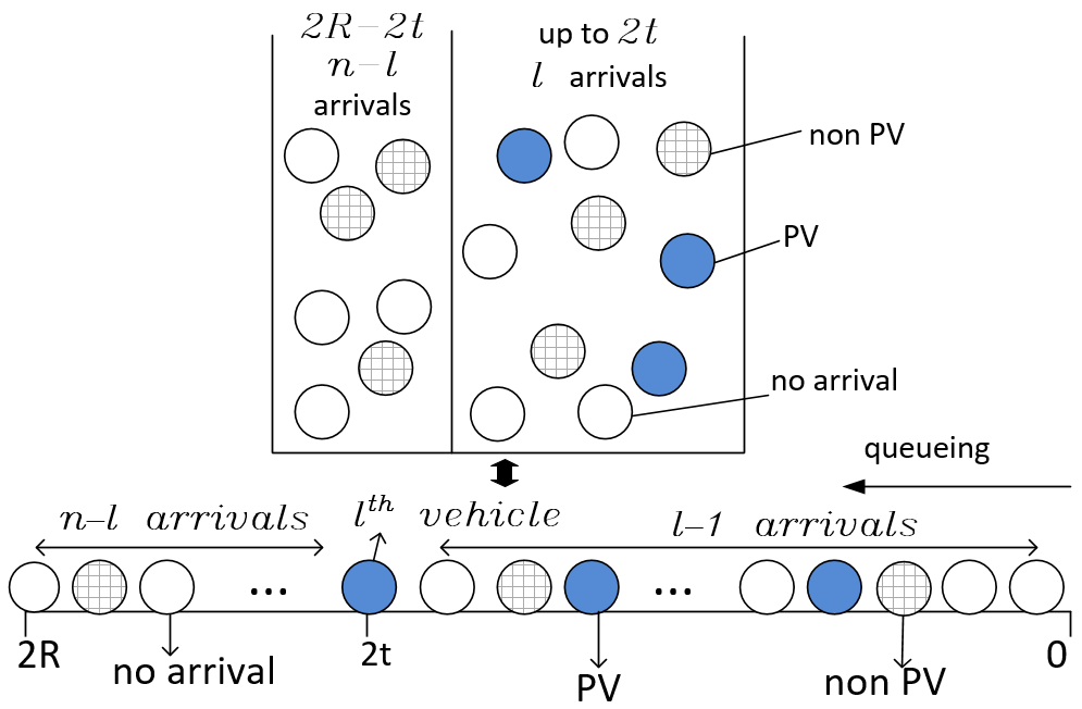
Fig. 1: Example queue with queue length, PV data, and arrival-no arrival spots

The problem is described on a single lane of approach and can equivalently be expressed as an urn modeling (see Fig. 1). Consider the approach lane queue formed in $2R$ (i.e., $R$ is red phase) time intervals where in one time interval there can be at most one arrival. So, in this set up there can be at most one arrival per $0.5$ seconds. This can be thought of as the minimum possible time gap and can be updated in the formulations derived. In Fig. 1, we have $l$ arrivals in $2t$ time intervals among these $2t-1$ contain $m-1$ CVs, $2R-2t$ has $n-l$ arrivals. Now, the problem is a negative inference, meaning $n$ is changing as in Negative Binomial, so, we are interested in $P(N=n|L=l,M=m,T=t,R)$, i.e., probability of having $N=n$ arrivals within $R$ time interval given $L=l,T=t,M=m$. Calculating this probability, we obtain Eq. (1) or equivalently Eq. (2).

$$\frac{\binom{2t}{l-m}\binom{2R-2t}{n-l}}{\binom{2R}{n-m}}$$ (1)

$$\frac{\binom{n-m}{l-m}\binom{2R-(n-m)}{2t-(l-m)}}{\binom{2R}{2t}}$$ (2)

We can then calculate expected values to get the mean ($E(n|l,t,m,R)$ or the queue length estimator) and the variance ($V(n|l,t,m,R)$) of the estimator. However, we first need to

1. verify if this is a valid probability mass function.

2. find the normalizing denominator for a valid probability mass function.

3. simplify to forms that can be used as input-output models like $E(n|l,t,m,R)=l+(1-p)\lambda(R-t)$ in (Comert (2013b)).

4. show if this approach leads to one of the known negative probability mass functions (e.g., Negative Hypergeometric). This could facilitate (iii).

3 Probability Mass Function, Expected Value, and Variance

We first provide combinatorial arguments and derive a closed-form for the sum of the function in Eq. (2).

Theorem 1

Let $\ell$, $t$, $R$, and $m$ be as defined in the preceding section. Then

$$\sum_{n=\ell}^{2R-2t+\ell}\frac{\binom{n-m}{\ell-m}\binom{2R+m-n}{2t+m-\ell}}{\binom{2R}{2t}}=\frac{2R+1}{2t+1}\\$$ (3)

or equivalently

$$\sum_{n=\ell}^{2R-2t+\ell}\binom{n-m}{\ell-m}\binom{2R+m-n}{2t+m-\ell}=\binom{2R+1}{2t+1}$$ (4)

Proof. Observe $\binom{n-m}{\ell-m}=\binom{n-m}{n-\ell}$ and $\binom{2R+m-n}{2t+m-\ell}=\binom{2R+m-n}{2R-2t-n+\ell}$ and replace $n^{\prime}=n-\ell$ so that Eq. (4) becomes

$$\sum_{n^{\prime}=0}^{2R-2t}\binom{n^{\prime}+\ell-m}{n^{\prime}}\binom{2R+m-n^{\prime}-\ell}{2R-2t-n^{\prime}}=\binom{2R+1}{2t+1}$$ (5)

Make another re-indexing $\ell^{\prime}=\ell-m$ and hence Eq. (5) takes the form

$$\sum_{n^{\prime}=0}^{2R-2t}\binom{n^{\prime}+\ell^{\prime}}{n^{\prime}}\binom{2R-\ell^{\prime}-n^{\prime}}{2R-2t-n^{\prime}}=\binom{2R+1}{2t+1}$$ (6)

The "negativization" (reminiscent of the Euler’s gamma reflection formula $\Gamma(z)\Gamma(1-z)=\frac{\pi}{\sin(\pi z)}$) of binomial coefficients $\binom{-a+b}{b}=(-1)^{b}\binom{a-1}{b}$ allows to convert $\binom{\ell^{\prime}+n^{\prime}}{n^{\prime}}=(-1)^{n^{\prime}}\binom{-\ell^{\prime}-1}{n^{\prime}}$ and $\binom{2R-\ell^{\prime}-n^{\prime}}{2R-2t-n^{\prime}}=\binom{2t-\ell^{\prime}+2R-2t-n^{\prime}}{2R-2t-n^{\prime}}=(-1)^{2R-2t-n^{\prime}}\binom{\ell^{\prime}-2t-1}{2R-2t-n^{\prime}}$. Therefore,

$$\sum_{n^{\prime}=0}^{2R-2t}\binom{n^{\prime}+\ell^{\prime}}{n^{\prime}}\binom{2R-\ell^{\prime}-n^{\prime}}{2R-2t-n^{\prime}}$$

$$=\sum_{n^{\prime}=0}^{2R-2t}\binom{-\ell^{\prime}-1}{n^{\prime}}\binom{\ell^{\prime}-2t-1}{2R-2t-n^{\prime}}$$ (7)

The well-known Vandermonde-Chu identity states $\sum_{k=0}^{y}\binom{x}{k}\binom{z}{y-k}=\binom{x+z}{y}$. Applying this to Eq. (3) and engaging $\binom{-a+b}{b}=(-1)^{b}\binom{a-1}{b}$ (one more time) yields

$$\sum_{n^{\prime}=0}^{2R-2t}\binom{-\ell^{\prime}-1}{n^{\prime}}\binom{\ell^{\prime}-2t-1}{2R-2t-n^{\prime}}=$$

$$\binom{-2t-2}{2R-2t}=(-1)^{2R-2t}\binom{2R+1}{2R-2t}=\binom{2R+1}{2t+1}$$

The proof is complete. $\square$

Remark. The identity just proved shows that Eq. (3) or Eq. (4) is independent of the parameters $m$ and $\ell$.

We can see that the identity proved in the above theorem enables us to revise Eq. (2) and define a probability mass function. We can divide both sides of the identity by the expression on the right-hand side of the identity to get one on the right-hand side (i.e., the right-hand side of the identity is the normalizer of the probability distribution, which we explain below). Note that additional results from combinatorics and discussions are presented in the Appendix.

In Negative Hypergeometric distribution (Johnson et al. (2005)), the probability of having $k$ successes up to the $r^{th}$ failure given sample size of $S$ and maximum possible queued vehicles $K$ is given by

$$p(k|r,K,S)=\frac{\binom{k+r-1}{k}\binom{S-r-k}{K-k}}{\binom{S}{K}}$$ (8)

where $S$ is the sample size (time capacity for arrivals and non-arrivals), $K$ is the total number of successes (arrivals) in $S$, $r$ is the number of failures (non-arrivals), and $k$ is the number of successes (realizations of arrivals). The probabilities sum to $1$. For the Negative Hypergeometric distribution, the expected value $E(k|r,K,S)$ and the variance $V(k|r,K,S)$ are given by Eqs. (9) and (10).

$$E(k|r,K,S)=\frac{rK}{S-K+1}$$ (9)

$$V(k|r,K,S)=\frac{rK(S+1)(S-K-r+1)}{(S-K+1)^{2}(S-K+2)}$$ (10)

In the probability mass function of the Negative Hypergeometric distribution (Eq. (8)), let $S=2R+1$, $K=2R-2t$, $r=l-m+1$, and $k=n-l$. Then the result proved in the theorem above gives the following probability mass function, which is a Negative Hypergeometric distribution since $\sum_{n=l}^{2R-2t+l}\binom{n-m}{l-m}\binom{2R+m-n}{2t+m-l}=\binom{2R+1}{2t+1}$. Notice that with these assignments arrivals and non-arrivals are fixed and probability of the total queue $N=n$ is calculated with known $l,m,t,R$.

$$p(N=n|l,m,t,R)=\frac{\binom{n-m}{l-m}\binom{2R+m-n}{2t+m-l}}{\binom{2R+1}{2t+1}}$$ (11)

From the formulas for the expected value and variance of the Negative Hypergeometric distribution, we get the following formulas for the expected value (Eq. (9)) and variance (Eq. (10)) of this probability distribution in Eq. (11). Note that $L=l,M=m,T=t,R$ are basic information from CVs, not primary parameters (arrival or penetration rate of probe vehicle in the traffic stream). We also do not require steady-state behavior if this Probe vehicle information is available. The expected queue length and its variance are short-term ($R$ seconds or time interval) estimators.

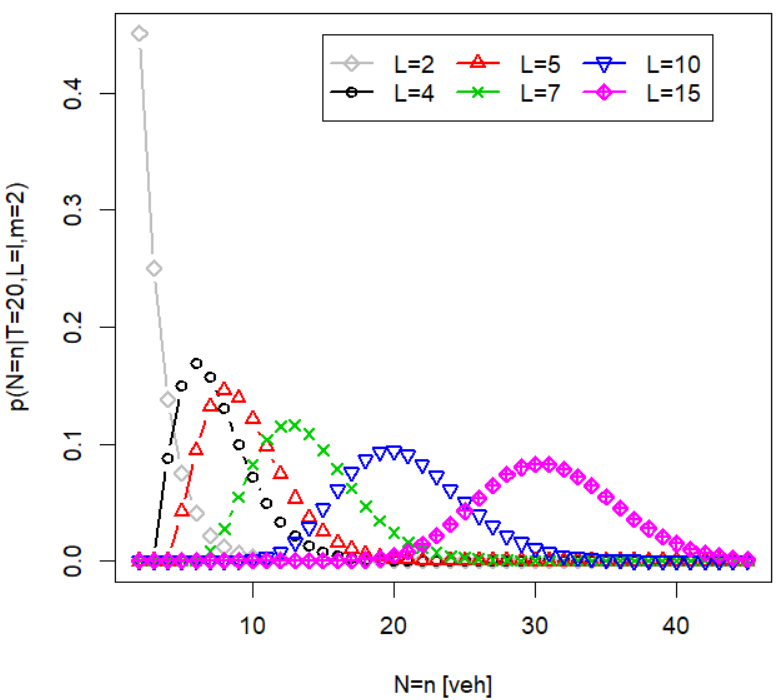
(a) $p(N|T=20,L,M=2,R=45)$ in Eq. (11)

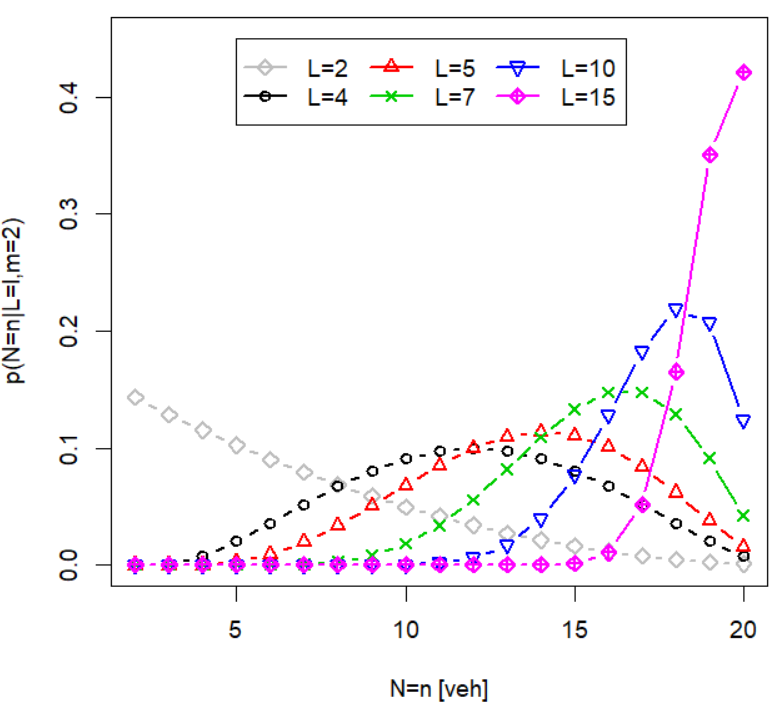
(b) $p(N|L,M=2,R=45)$ in Eq. (14)

Fig. 2: Example behavior of conditional probabilities

The expected value $E(n|l,t,m,R)$ can be determined by

$$E(N|l,m,t,R) = \sum_{n=l}^{2R-2t+l}{\frac{n(2R+1)}{(2t+1)}\frac{\binom{n-m}{l-m}\binom{2R+m-n}{2t+m-l}}{\binom{2R+1}{2t+1}}}$$

$$= \sum_{n^{\prime}=0}^{2R-2t}{\frac{n^{\prime}(2R+1)}{(2t+1)}\frac{\binom{n^{\prime}+l^{\prime}}{n^{\prime}}\binom{2R-l^{\prime}-n^{\prime}}{2R-2t-n^{\prime}}}{\binom{2R+1}{2t+1}}}$$

where $n^{\prime}=n-l$, $l^{\prime}=l-m$, and $\frac{(2R+1)}{(2t+1)}$ is the normalizer.

By Eqs. (9) and (10), simplified expected value or the queue length estimation 1 and the variance can be obtained as in Eqs. (12) and (13).

$$E(N_{1}=n_{1}|l,m,t,R) = l+\frac{(l-m+1)(2R-2t)}{2t+2}$$ (12)

$$= l+\frac{(l-m+1)(R-t)}{t+1}$$

$$V(N_{1}=n_{1}|l,m,t,R)= \frac{(l-m+1)(2R+2)(2R-2t)}{(2t+2)(2t+3)}[1-\frac{l-m+1}{2t+2}]$$ (13)

Alternatively, from Eq. (14), we can get the following equivalent estimator without CV time ($T$) information (Eq. (15)) and its variance in (Eq. (16)).

$$p(N=n|l,m,C)=\frac{\binom{C-n+m}{C-n}\binom{n-m}{n-l}}{\binom{C}{l}}$$ (14)

where $C$ is capacity or maximum possible arrivals, $J=C-2l$, $r=l-m+1$, $K=C-l$, and $k=n-l$. Note that, with time discretization, we can infer $t$ from $l$. The expected value $E(n|l,m,R)$ is given by

$$E(N=n|l,m,R) = \sum_{n=l}^{C+l}{\frac{n(l+1)}{(C+1)}\frac{\binom{C-n+m}{C-n}\binom{n-m}{n-l}}{\binom{C}{l}}}$$

$$= \sum_{n^{\prime}=0}^{C}{\frac{n^{\prime}(l+1)}{(C+1)}\frac{\binom{n^{\prime}+l^{\prime}}{n^{\prime}}\binom{C-l^{\prime}+n^{\prime}}{C-l^{\prime}-n^{\prime}}}{\binom{C}{n^{\prime}}}}$$

where $n^{\prime}=n-l$, $l^{\prime}=l-m$, and $\frac{(l+1)}{(C+1)}$ is the normalizer for valid probability mass function.

$$E(N_{2}=n_{2}|l,m,C)=l+\frac{(l-m+1)(C-l)}{l+2}$$ (15)

$$V(N_{2}=n_{2}|l,m,C)=\frac{(l-m+1)(C+2)(C-l)}{(l+2)(l+3)}[1-\frac{l-m+1}{l+2}]$$ (16)

One of the advantages of the derived estimators in Eqs. (12) and (15) is that the denominators are nonzero since $L\geq 0$. This enables us to estimate queues even if there is no probe vehicle in the queue. The behavior of conditional probabilities, expected values, and variances are shown in Figs. 2-4. We can see in Fig. 2 that the likelihoods are right to the $N=l$ values. In Fig. 3, as queue time joining of the last probe vehicle increases, then the expected queue length gets closer to $L=l$ for both models. Similarly, in Fig. 4, the variance of the estimated queue length reduces as $l$ and $t$ increase. Having time information also shows smoother behavior compared to having only location information.

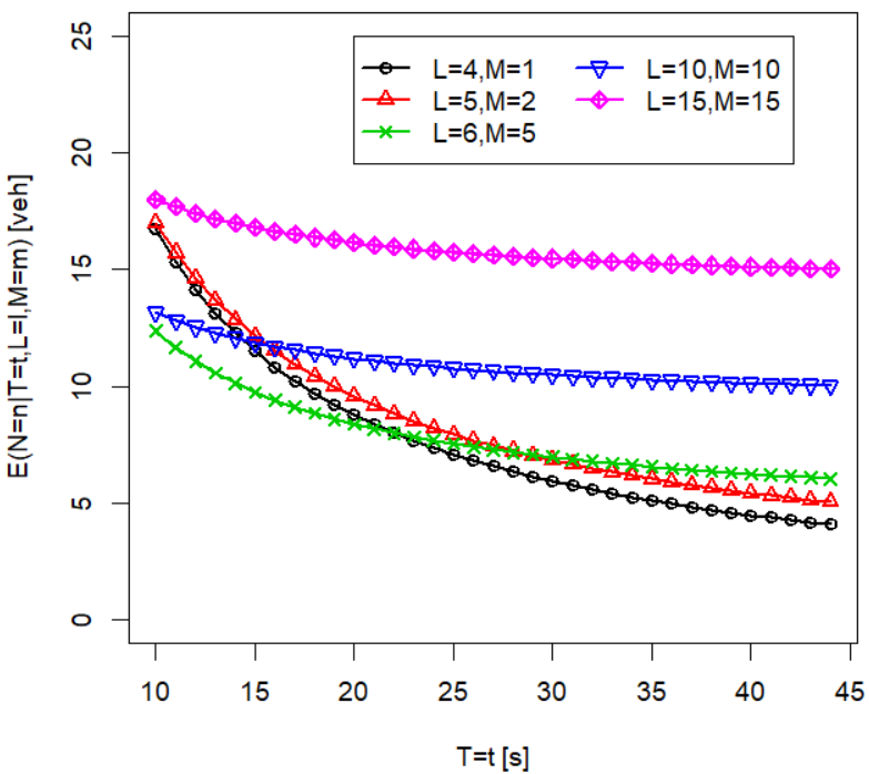
(a) $E(N|T,L,M=2,R=45)$ in Eq. (12)

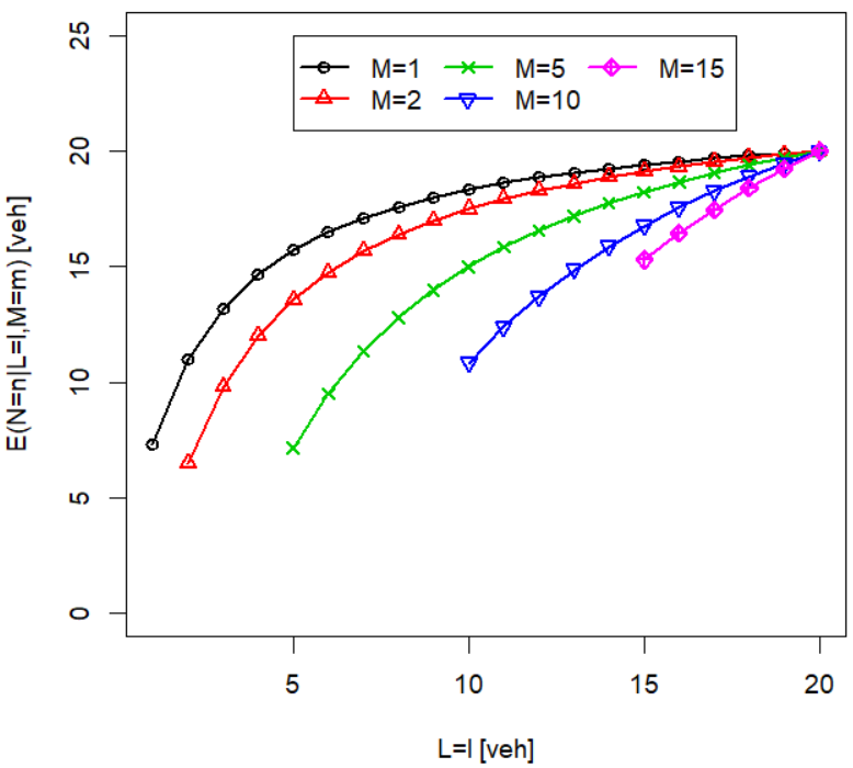
(b) $E(N|L,M,R=45)$ in Eq. (15)

Fig. 3: Example behavior of conditional expectations

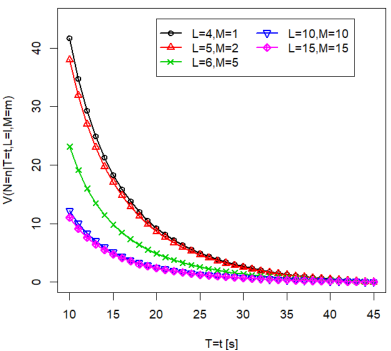
(a) $V(N|T,L,M=2,R=45)$ in Eq. (12)

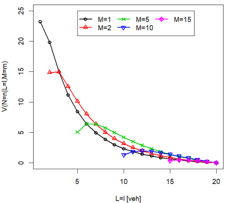
(b) $V(N|L,M,R=45)$ in Eq. (16)

Fig. 4: Example behavior of conditional variances

4 Evaluation with Field Queue Length Data

To show the effectiveness of the estimators developed, we used 2014 ITS World Congress Connected Vehicle Demonstration Data (Dataset (2014)). Authors’ previous works used this field data for evaluating range sensor inclusion and filtering for queue length estimation (Comert and Begashaw (2021); Comert and Cetin (2021)). Results for this study are new. For completeness, assumptions and set up are reported again. The dataset contains manually collected queue lengths at the intersection of Larned and Shelby streets in Detroit, Michigan, between September $8$ and $10$, $2014$. The number of observations per day are $98$, $254$, and $135$, respectively. During data collection, probe vehicles were identified with the blue $X$s. Each row of data includes hour, minute, second of an observation, the maximum queue lengths, and the number of probe vehicles in these queues (i.e., $M$ in the formulations above) from left, center, and right lanes of Larned street approach.

The dataset provides $M=m$ and $C$ cycle time values but not the information of $L$ and $T$ from PVs. Hence, we generated random variates of this information from Uniform ($L=l$ location $l\sim U(m,n)$) and Gamma ($T=t$ queue joining time $t\sim\mathcal{G}a(l,\frac{C}{2n})$) distributions for all lanes independently and repeated for $1000$ random seeds. Note that, integer values are used for $L,M$, and $T$. Overall average of estimation errors are reported to compare models. In addition, followings are assumed related to the traffic signal and the dataset:

1. Back of queue observations are obtained at the end of red phases (vary cycle-by-cycle). The time between two observations is assumed to be the cycle length ($C$) and red phases are assumed to be half ($R=C/2$).

2. There is no steady growth of queue and many zero queue values. Thus, the overflow queues are omitted . The data was collected during low to medium $\rho$ (i.e., volume-to-capacity ratio$=0.50$). Regardless, $\rho$s are also calculated using estimated arrival rates.

3. The capacity of the approach was approximated by the observed overall maximum queue value of $10$ vehicles within $70$ seconds ($10\times 3600/35$=$1029$ vehicles per hour or $0.286$ vehicles per second ($vps$) saturation flow rate). These values are used essentially in the Highway Capacity Manual (HCM) from a manual and back of queue calculations. Note that the values may not be reflecting actual capacity and phase splits; however, we compare and report against true queue lengths. This would provide insights into the accuracy of our approach.

Compared HCM delay (i.e., $Delay$) and back of queue (i.e., $Q{back}$) models are given in Eqs. (4) and (18). These models are approximations for given time intervals (e.g., $15$ minutes) and fully observed traffic.

$$d_{1}=\frac{C}{2}[\frac{(1-G/C)^{2}}{1-[min(1,\hat{X})G/C]}]$$

$$d_{2}=900T[(\hat{X}-1)+\sqrt{(\hat{X}-1)^{2}+\frac{8kI\hat{X}}{cT}}]$$ (17)

where $d$=$d_{1}\times PF+d_{2}+d_{3}$ is control delay seconds per vehicle, $d_{2}$ is uniform delay, $PF$ is progression factor due to arrival types, $d_{2}$ is random delay component, and $d_{3}$ is delay due to initial queue. In this study, only $d_{1}+d_{2}$ are considered with $d_{3}=0$ since no overflow queue is assumed. $PF=1.0$ is used for random arrivals. Volume-to-capacity is $\hat{X}=\hat{\rho}=\frac{\hat{\lambda}}{0.286}$. Green time $G$ is in seconds $s$, $C$ is cycle time in $s$. $T$ is the analysis period in hours where in cycle-to-cycle estimations $T_{i}=C_{i}/3600$ is assumed where $i$ denotes cycle number. $k$ is incremental delay factor, and $0.5$ is assumed for fixed time like movement. $I=1$ upstream filtering is assumed for no interaction with nearby intersections, and capacity is $c=1029$ $vph$. Note that in our calculations, uniform delay is the main component updated by changing $G$ and $C$ values. Queue lengths are approximated by Little’s formula $d\lambda$ where $d$ and $\lambda$ are both calculated at each cycle using $M$ number of probe vehicles in the queue. This method is based on HCM 2000 (Prassas and Roess (2020); Ni (2020)).

Another estimation approach adopted from (Kyte et al. (2014)) that is used to calculate cycle-to-cycle back of queues (see Eq. (18)).

$$Q_{back}=\hat{v}(R+g_{s})$$ (18)

where, $Q_{back}$ is back of the queue in vehicles, $v=\lambda$ is arrival rate in vehicles per second ($vps$), $R$ is the red duration in seconds $s$, and $g_{s}$ is queue service time that is calculated $\hat{v}R/(x-\hat{v})$ with $x$ is the saturation flow rate (i.e., assumed to be $0.286$ vps). All the values $R$, $g_{s}$, and $\hat{v}$ except $x$ are changing cycle-to-cycle.

Alternative estimators from Comert (2016) are denoted by Est.1 and Est.2 in Eqs. (19) and (4), respectively. These queue length estimators are in the form of $E(n|l,m,t,R)=l+(1-\hat{p})\hat{\lambda}(R-t)$ with two different primary parameter estimator combinations: $\{\hat{\lambda}_{1}=\frac{l}{R},\hat{p}_{1}=\frac{m}{l}\}$ and $\{\hat{\lambda}_{2}=\frac{(l-m)}{t}+\frac{m}{R},\hat{p}_{2}=\frac{mt}{mt+(l-m)R}\}$.

$$E(N_{1}|l,m,t,R)=I(m>0)[l+(l-m)(1-\frac{t}{R})]+I(m=0)[(1-\frac{\bar{m}}{\bar{l}})(\bar{l}+(\bar{l}-\bar{m})(1-\frac{\bar{t}}{R}))]$$ (19)

$$E(N_{2}|l,m,t,R)=I(m>0)[m+\frac{R(l-m)}{t}]+I(m=0)[(1-\frac{\bar{m}\bar{t}}{\bar{m}\bar{t}+(\bar{l}-\bar{m})R})(\bar{m}+\frac{R(\bar{l}-\bar{m})}{\bar{t}})]$$

$$\centering=I(m>0)[m+\frac{(l-m)R}{t}]+I(m=0)[\bar{m}+\frac{(\bar{l}-\bar{m})R}{\bar{t}}]\@add@centering$$ (20)

where $I(.)$ is the indicator function. When there is no probe vehicle in the queue (i.e., $I(m=0)$), we use the average of previous probe vehicles’ information as we need to estimate arrival rate ($\lambda$) and probe percentage ($p$). Notation $M_{1:i}$ represents values from cycle $1$ to $i$ and $\bar{m}_{1:i}=\sum_{j=1}^{i}{\frac{m_{j}}{i}}$, $\bar{l}_{1:i}=\sum_{j=1}^{i}{\frac{l_{j}}{i}}$, and $\bar{t}_{1:i}=\sum_{j=1}^{i}{\frac{t_{j}}{i}}$. Average error values are given in Table 1 for $T\sim\mathcal{G}a(l,\frac{C}{2n})$. Fig. 5(b) is given to demonstrate if assumed interarrivals are impacting the accuracy of the estimators.

Table 1: Estimation results with RMSE errors in [vehs/cycle] with $T\sim\mathcal{G}a(l,$C$/(2n))$

	Lane	Avg. $p$	Est.1	Est.2	NP.Est.1	NP.Est.2	Delay	Q back
Sep08	L	13%	1.09	1.01	1.01	1.01	1.37	1.25
	C	21%	0.72	0.78	0.69	0.70	1.33	1.26
	R	7%	0.56	0.55	0.60	0.60	0.66	0.64
Sep09	L	10%	1.22	1.05	0.99	0.99	1.38	1.13
	C	26%	1.14	0.96	1.09	1.09	1.81	1.38
	R	2%	0.34	0.35	0.54	0.54	0.39	0.41
Sep10	L	7%	2.68	2.43	2.48	2.48	2.81	2.52
	C	18%	1.48	1.32	1.73	1.73	2.28	1.63
	R	1%	0.84	0.77	0.77	0.77	1.06	1.26

In Table 1, a summary of average queue length ($QL$) estimation errors in the root mean square is provided (RMSE=$\sqrt{\sum_{i=1}^{n}{\frac{(QL_{i}-\hat{QL}_{i})^{2}}{n}}}$). Average $p$ values are calculated from $\sum_{i=1}^{n}{\frac{m}{nQL_{i}}}$ for each lane. Since true maximum queues are not known, $p$ and $\lambda$ are estimated. HCM’s control delay-based model and back of queue are denoted by $HCM_{d}$ and $Q_{back}$, respectively. The accuracy of the estimators is reported when probe vehicles are present in the queue ($p$=$\{10\%,13\%,18\%,21\%$, $26\%\}$).

Example performances with $21\%$ penetration rates is given in Fig. 5(a). When there are probe vehicles in the queue, we can see that the proposed methods can follow the true maximum queue lengths closely. In Fig. 5(b), boxplots for overall errors are given. We can see that the model with new estimators provides slightly lower errors. However, errors are lower than delay-based $HCM_{d}$ and $Q_{back}$ methods. Our methods can estimate more accurately compared to $Q_{back}$.

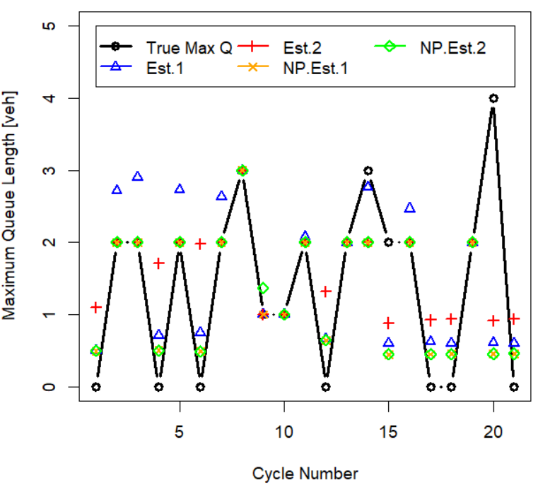
(a) Estimation on Sep 08 on center-lane

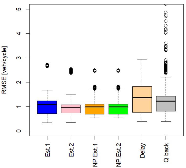
(b) Box plots for all estimation errors

Fig. 5: Performance of the proposed estimators $NP.Est.1$ and $NP.Est.2$

5 Conclusions

In this study, we derived two new nonparametric queue length estimation models for traffic signal-induced queues. The estimators only depend on signal phasing and timing information. The derivations involved fundamental experiment setup, and the resulting estimators were simple algebraic expressions. We did not assume independent arrivals at the intersection. The only assumption we made was discrete time intervals which are reasonable as signal timing involves whole seconds; in fact, multiples of five seconds.

For independent approach lanes at traffic intersections, it is shown that conditional queue lengths given probe vehicle location, count, time, and analysis interval can be represented by a Negative Hypergeometric distribution. The performance of the estimators derived was compared with parametric and simple highway capacity manual methods that use field test data involving probe vehicles. The results obtained from the comparisons show that the nonparametric models presented in this paper match the accuracy of parametric models. The methods developed do not assume random arrivals of vehicles at the intersection or any primary parameters or involve parameter estimations.

In this study, we developed methods to estimate queue length at intersection approaches from probe vehicles. These probe vehicles could be traditional probe vehicles or connected vehicles that generate basic safety messages. Future research could study the models presented in this paper to a more complex intersection and a series of adjacent intersections with large traffic demand volume at these intersections.

Appendix

The results in Eq. (1) can be extended to the short sum runs from $n=\ell$ through $n=2R-2t$.

Theorem 2

Let $\ell$, $m$, $n$, $R$, and $t$ be as defined in Theorem 1. Then there is a recurrence formula for

$$\sum_{n=\ell}^{2R-2t}\binom{n-m}{\ell-m}\binom{2R+m-n}{2t+m-\ell}.\quad(5)$$

Proof. Denote the sum by $f(\ell)$ and the summand by $F(\ell,n)$ (after suppressing the remaining variables). Introduce the function $G(\ell,n)=-\binom{n-m}{\ell+1-m}\binom{2R+m-n+1}{2t+m-\ell}$. Then, it is routine to verify that

$$F(\ell+1,n)-F(\ell,n)=G(\ell,n+1)-G(\ell,n).\quad(6)$$

Sum both sides of (6) for $n=\ell+1$ to $n=2R-2t$ (and telescoping on the right-hand side) to obtain

$$f(\ell+1)-f(\ell)+F(\ell,\ell)=G(\ell,2R-2t+1)-G(\ell,\ell+1).$$

Based on $F(\ell,\ell)=\binom{2R+m-\ell}{2t+m-\ell},G(\ell,2R-2t+1)=-\binom{2R-2t-m+1}{\ell-m+1}\binom{2t+m}{\ell}$ and $G(\ell,\ell+1)=-\binom{2R+m-\ell}{2t+m-\ell}$, we infer the recursive relation

$$f(\ell+1)-f(\ell)=-\binom{2R-2t-m+1}{\ell-m+1}\binom{2t+m}{\ell}.\qquad\square$$

Corollary. From Theorem 2, we get the following identity

$$\sum_{\ell=0}^{2R-2t}\binom{2R-2t-m+1}{\ell-m+1}\binom{2t+m}{\ell}=\binom{2R+1}{2t+1}.\quad(7)$$

Proof. This follows from the recurrence relation proved in Theorem 2 and the identity proved in Theorem 1. $\square$

Theorem 3

The identity in (7) can be re-indexed and formulated as follows:

$$\sum_{m=\ell}^{R-t+\ell}{m\choose\ell}{R-m\choose t-\ell}={R+1\choose t+1}.$$

Proof. We offer a combinatorial argument. Given natural numbers $\ell\leq t\leq R$, and $m$, we may consider the class of those $(t+1)$-subsets $\{x_{0}<x_{1}<\dots<x_{t}\}$ of $\{0,1,\dots,R\}$ such that $x_{\ell}=m$: these are exactly ${m\choose\ell}{R-m\choose t-\ell}$ (indeed the $\ell$ elements $x_{0},\dots,x_{\ell-1}$ can be chosen freely into $\{0,\dots,m-1\}$, and so can the $t-\ell$ elements $x_{\ell+1},\dots,x_{t}$ into $\{m+1,\dots,R\}$. These classes, for $\ell\leq m\leq R-t+\ell$ form a partition of all $(t+1)$-subsets of $[R+1]$, whence the sum of their cardinality is independent of $\ell$ and the identity. $\square$

Remark. The discrepancy in having a closed form and no closed form can be understood as follows: we know that $\sum_{k=0}^{n}\binom{n}{k}=2^{n}$, however there is no "nice evaluation" for $\sum_{k=0}^{m}\binom{n}{k}$ unless $m=n$. The bottom line is the former is summed over the full compact support of $\binom{n}{k}$ (in the sense, $\binom{n}{k}=0$ if $k<0$ or $k>n$. A similar analogy can be drawn with having the closed form $\int_{\mathbb{R}}e^{-x^{2}}dx=\sqrt{\pi}$ but nothing similar is available if the limit are altered to be any smaller subset than the full range $\mathbb{R}$, except for $[0,\infty)$.

References

- Bae et al. (2019) Bae, B., Liu, Y., Han, L.D., Bozdogan, H., 2019. Spatio-temporal traffic queue detection for uninterrupted flows. Transportation Research Part B: Methodological 129, 20–34.
- Comert (2013a) Comert, G., 2013a. Effect of stop line detection in queue length estimation at traffic signals from probe vehicles data. European Journal of Operational Research 226, 67–76.
- Comert (2013b) Comert, G., 2013b. Simple analytical models for estimating the queue lengths from probe vehicles at traffic signals. Transportation Research Part B: Methodological 55, 59–74.
- Comert (2016) Comert, G., 2016. Queue length estimation from probe vehicles at isolated intersections: Estimators for primary parameters. European Journal of Operational Research 252, 502–521.
- Comert and Begashaw (2021) Comert, G., Begashaw, N., 2021. Cycle-to-cycle queue length estimation from connected vehicles with filtering on primary parameters. International Journal of Transportation Science and Technology URL: https://www.sciencedirect.com/science/article/pii/S2046043021000319, doi:https://doi.org/10.1016/j.ijtst.2021.04.009.
- Comert and Cetin (2009) Comert, G., Cetin, M., 2009. Queue length prediction from probe vehicle location and the impacts of sample size. European Journal of Operational Research 197, 196–202.
- Comert and Cetin (2021) Comert, G., Cetin, M., 2021. Queue length estimation from connected vehicles with range measurement sensors at traffic signals. Applied Mathematical Modelling 99, 418–434.
- Dataset (2014) Dataset, C., 2014. ITS World Congress Connected Vehicle Test Bed Demonstration Vehicle Situation Data. South East Michigan Test Bed Contractor Team, Noblis’ Queue Length Algorithm Development Team, and Data Capture and Management Data Sets Contractor Team, provided by ITS DataHub through Data.transportation.gov. URL: Accessed2021-01-25fromhttp://doi.org/10.21949/1504496.
- Duret and Yuan (2017) Duret, A., Yuan, Y., 2017. Traffic state estimation based on eulerian and lagrangian observations in a mesoscopic modeling framework. Transportation research part B: methodological 101, 51–71.
- Florin and Olariu (2020) Florin, R., Olariu, S., 2020. Towards real-time density estimation using vehicle-to-vehicle communications. Transportation research part B: methodological 138, 435–456.
- Gao et al. (2019) Gao, K., Han, F., Dong, P., Xiong, N., Du, R., 2019. Connected vehicle as a mobile sensor for real time queue length at signalized intersections. Sensors 19, 2059.
- Goldenshluger (2016) Goldenshluger, A., 2016. Nonparametric estimation of the service time distribution in the m/g/∞ queue. Advances in Applied Probability 48, 1117–1138.
- Goldenshluger and Koops (2019) Goldenshluger, A., Koops, D.T., 2019. Nonparametric estimation of service time characteristics in infinite-server queues with nonstationary poisson input. Stochastic Systems 9, 183–207.
- Hans et al. (2015) Hans, E., Chiabaut, N., Leclercq, L., 2015. Applying variational theory to travel time estimation on urban arterials. Transportation Research Part B: Methodological 78, 169–181.
- Herrera and Bayen (2010) Herrera, J.C., Bayen, A.M., 2010. Incorporation of lagrangian measurements in freeway traffic state estimation. Transportation Research Part B: Methodological 44, 460–481.
- Jenelius and Koutsopoulos (2013) Jenelius, E., Koutsopoulos, H.N., 2013. Travel time estimation for urban road networks using low frequency probe vehicle data. Transportation Research Part B: Methodological 53, 64–81.
- Jenelius and Koutsopoulos (2015) Jenelius, E., Koutsopoulos, H.N., 2015. Probe vehicle data sampled by time or space: Consistent travel time allocation and estimation. Transportation Research Part B: Methodological 71, 120–137.
- Jin and Ma (2019) Jin, J., Ma, X., 2019. A non-parametric bayesian framework for traffic-state estimation at signalized intersections. Information Sciences 498, 21–40.
- Johnson et al. (2005) Johnson, N.L., Kemp, A.W., Kotz, S., 2005. Univariate discrete distributions. volume 444. John Wiley & Sons.
- Kyte et al. (2014) Kyte, M., Tribelhorn, M., et al., 2014. Operation, analysis, and design of signalized intersections: a module for the introductory course in transportation engineering. Technical Report. TranLIVE. University of Idaho.
- Ni (2020) Ni, D., 2020. Signalized Intersections. Springer.
- Prassas and Roess (2020) Prassas, E.S., Roess, R.P., 2020. The Highway Capacity Manual: A Conceptual and Research History Volume 2. Springer.
- Ramezani and Geroliminis (2012) Ramezani, M., Geroliminis, N., 2012. On the estimation of arterial route travel time distribution with markov chains. Transportation Research Part B: Methodological 46, 1576–1590.
- Schweer and Wichelhaus (2015) Schweer, S., Wichelhaus, C., 2015. Nonparametric estimation of the service time distribution in the discrete-time gi/g/∞ queue with partial information. Stochastic Processes and their Applications 125, 233–253.
- Seo et al. (2019) Seo, T., Kawasaki, Y., Kusakabe, T., Asakura, Y., 2019. Fundamental diagram estimation by using trajectories of probe vehicles. Transportation Research Part B: Methodological 122, 40–56.
- Singh et al. (2021) Singh, S.K., Acharya, S.K., Cruz, F.R., Quinino, R.C., 2021. Estimation of traffic intensity from queue length data in a deterministic single server queueing system. Journal of Computational and Applied Mathematics , 113693.
- Tan et al. (2020) Tan, C., Liu, L., Wu, H., Cao, Y., Tang, K., 2020. Fuzing license plate recognition data and vehicle trajectory data for lane-based queue length estimation at signalized intersections. Journal of Intelligent Transportation Systems , 1–18.
- Wang et al. (2013) Wang, W., Bengler, K., Wets, G., Niu, H., 2013. Modeling and simulation in transportation engineering. Mathematical Problems in Engineering 2013, 1–2.
- Wang et al. (2020) Wang, Z., Zhu, L., Ran, B., Jiang, H., 2020. Queue profile estimation at a signalized intersection by exploiting the spatiotemporal propagation of shockwaves. Transportation research part B: methodological 141, 59–71.
- Wong et al. (2019) Wong, W., Shen, S., Zhao, Y., Liu, H.X., 2019. On the estimation of connected vehicle penetration rate based on single-source connected vehicle data. Transportation Research Part B: Methodological 126, 169–191.
- Zhao et al. (2021a) Zhao, Y., Shen, S., Liu, H.X., 2021a. A hidden markov model for the estimation of correlated queues in probe vehicle environments. Transportation Research Part C: Emerging Technologies 128, 103128.
- Zhao et al. (2021b) Zhao, Y., Wong, W., Zheng, J., Liu, H.X., 2021b. Maximum likelihood estimation of probe vehicle penetration rates and queue length distributions from probe vehicle data. IEEE Transactions on Intelligent Transportation Systems .
- Zhao et al. (2019) Zhao, Y., Zheng, J., Wong, W., Wang, X., Meng, Y., Liu, H.X., 2019. Various methods for queue length and traffic volume estimation using probe vehicle trajectories. Transportation Research Part C: Emerging Technologies 107, 70–91.
- Zheng et al. (2018) Zheng, F., Jabari, S.E., Liu, H.X., Lin, D., 2018. Traffic state estimation using stochastic lagrangian dynamics. Transportation Research Part B: Methodological 115, 143–165.