A Simple Algorithm for Graph Reconstruction

Abstract

How efficiently can we find an unknown graph using distance queries between its vertices? We assume that the unknown graph is connected, unweighted, and has bounded degree. The goal is to find every edge in the graph. This problem admits a reconstruction algorithm based on multi-phase Voronoi-cell decomposition and using $\tilde{O}(n^{3/2})$ distance queries [27].

In our work, we analyze a simple reconstruction algorithm. We show that, on random $\Delta$-regular graphs, our algorithm uses $\tilde{O}(n)$ distance queries. As by-products, we can reconstruct those graphs using $O(\log^{2}n)$ queries to an all-distances oracle or $\tilde{O}(n)$ queries to a betweenness oracle, and we bound the metric dimension of those graphs by $\log^{2}n$.

Our reconstruction algorithm has a very simple structure, and is highly parallelizable. On general graphs of bounded degree, our reconstruction algorithm has subquadratic query complexity.

1 Introduction

Discovering the topology of the Internet is a crucial step for building accurate network models and designing efficient algorithms for Internet applications. The topology of Internet networks is typically investigated at the router level, using traceroute. It is a common and reasonably accurate assumption that traceroute generates paths that are shortest in the network. Unfortunately, sometimes routers block traceroute requests due to privacy and security concerns. As a consequence, the inference of the network topology is rather based on the end-to-end delay information on those requests, which is roughly proportional to the shortest-path distances in the network.

In the graph reconstruction problem, we are given the vertex set $V$ of a hidden connected, undirected, and unweighted graph and have access to information about the topology of the graph via an oracle, and the goal is to find every edge in $E$. Henceforth, unless explicitly mentioned, all graphs studied are assumed to be connected. This assumption is standard and shared by almost all references on the subject, e.g., [7, 14, 27, 39, 41]. The efficiency of an algorithm is measured by the query complexity, i.e., the number of queries to the oracle. Motivated by traceroute, the literature has explored several types of query oracles.

• One type consists of all-shortest-paths and all-distances queries, when querying a vertex yields either shortest paths from that vertex to all other vertices [7, 41] or distances from that vertex to all other vertices [14]. The latter, of course, is less informative.

• A more refined type of query oracles, suggested in [7, 14], consists of shortest-path and distance queries, when querying a pair of vertices yields either a shortest path or the distance between them [27, 38, 39]. Again, the latter is less informative.

In this work, we focus on the weakest of those four query oracles, that takes as input a pair of vertices $a$ and $b$ and returns the distance $\delta(a,b)$ between them. Reyzin and Srivastava [38] showed that graph reconstruction requires $\Omega(n^{2})$ distance queries on general graphs, so we focus on the bounded degree case. For graphs of bounded degree, Kannan, Mathieu, and Zhou [27] gave a reconstruction algorithm based on multi-phase Voronoi-cell decomposition and using $\tilde{O}(n^{3/2})$ distance queries, and raised an open question of whether $\tilde{O}(n)$ is achievable.

We provide a partial answer to that open question by analyzing a simple reconstruction algorithm (Algorithm 1). We show that, on (uniformly) random $\Delta$-regular graphs, where every vertex has the same degree $\Delta$, our reconstruction algorithm uses $\tilde{O}(n)$ distance queries (Theorem 1.1). As by-products, we can reconstruct those graphs using $O(\log^{2}n)$ queries to an all-distances oracle (Corollary 1.2) or using $\tilde{O}(n)$ queries to a betweenness oracle (Corollary 1.3), and we bound the metric dimension of those graphs by at most $\log^{2}n$ (Corollary 1.5).

Our analysis exploits the locally tree-like property of random $\Delta$-regular graphs, meaning that these graphs contain a small number of short cycles. Our method might be applicable to other locally tree-like graphs, such as Erdös-Rényi random graphs and scale-free graphs. In particular, many real world networks, such as Internet networks, social networks, and peer-to-peer networks, are believed to have scale-free properties [6, 25, 34]. We defer the reconstruction of those networks for future work.

Our reconstruction algorithm has a very simple structure, and is highly parallelizable (Corollary 1.4). On general graphs of bounded degree, the same reconstruction algorithm has subquadratic query complexity (Theorem 1.6).

1.1 Related Work

The problem of reconstructing a graph using queries that reveal partial information has been extensively studied in different contexts and has many applications.

Reconstruction of Random Graphs

The gist of our paper deals with random graphs. The graph reconstruction problem has already attracted much interest in the setting of random graphs. On Erdös-Rényi random graphs, Erlebach, Hall, and Mihal’ák [15] studied the approximate network reconstruction using all-shortest-paths queries; Anandkumar, Hassidim, and Kelner [4] used end-to-end measurements between a subset of vertices to approximate the network structure. Experimental results to reconstruct random graphs using shortest-path queries were given in [8, 20].

On random $\Delta$-regular graphs, Achlioptas et al. [2] studied the bias of traceroute sampling in the context of the network reconstruction. They showed that the structure revealed by traceroute sampling on random $\Delta$-regular graphs admits a power-law degree distribution [2], a common phenomenon as in Erdös-Rényi random graphs [31] and Internet networks [16].

Metric Dimension and Related Problems

Our work yields an upper bound on the metric dimension of random $\Delta$-regular graphs. The metric dimension problem was first introduced by Slater [42] and Harary and Melter [21], see also [5, 12, 13, 23, 29, 36, 37, 40]. The metric dimension of a graph is the cardinality of a smallest subset $S$ of vertices such that every vertex in the graph has a unique vector of distances to the vertices in $S$. On regular graphs, the metric dimension problem was studied in special cases [13, 24]. In Erdös-Rényi random graphs, the metric dimension problem was studied by Bollobás, Mitsche, and Prałat [11]. Mitsche and Rué [32] also considered the random forest model.

A related problem is the identifying code of a graph [28], which is a smallest subset of vertices such that every vertex of the graph is uniquely determined by its neighbourhood within this subset. The identifying code problem was studied on random $\Delta$-regular graphs [17] and on Erdös-Rényi random graphs [19]. Other related problems received attentions on random graphs as well, such as the sequential metric dimension [35] and the seeded graph matching [33].

Betweenness Oracle

There exists an oracle that is even weaker than the distance oracle: the betweenness oracle [1], which receives three vertices $u$, $v$, and $w$ and returns whether $w$ lies on a shortest path between $u$ and $v$. Our work yields a reconstruction algorithm using $\tilde{O}(n)$ betweenness queries on random $\Delta$-regular graphs. For graphs of bounded degree, Abrahamsen et al. [1] generalized the $\tilde{O}(n^{3/2})$ result in the distance oracle model from [27] to the betweenness oracle model.

Tree Reconstruction and Parallel Setting

Our paper focuses on the distance oracle and bounded degree, and considers the parallel setting. All of those aspects were previously raised in the special case of the tree reconstruction. Indeed, motivated by the reconstruction of a phylogenetic tree in evolutionary biology, the tree reconstruction problem using a distance oracle is well-studied [22, 30, 43], in particular assuming bounded degree [22]. Afshar et al. [3] studied the tree reconstruction in the parallel setting, analyzing both the round complexity and the query complexity in the relative distance query model [26].

1.2 Our Results

Our reconstruction algorithm, called Simple, is given in Algorithm 1. It takes as input the vertex set $V$ of size $n$ and an integer parameter $s\in[1,n]$.

Algorithm 1 Simple $(V,s)$

1:$S\leftarrow$ sample of $s$ vertices selected uniformly and independently at random from $V$

2:for $u\in S$ and $v\in V$ do Query$(u,v)$

3:$\hat{E}\leftarrow$ set of vertex pairs $\{a,b\}\subseteq V$ such that, for all $u\in S$, $|\delta(u,a)-\delta(u,b)|\leq 1$

4:for $\{a,b\}\in\hat{E}$ do Query$(a,b)$

5:return set of vertex pairs $\{a,b\}\in\hat{E}$ such that $\delta(a,b)=1$

Intuitively, the set $\hat{E}$ constructed in Simple consists of all vertex pairs $\{a,b\}\subseteq V$ that might be an edge in $E$. In order to obtain the edge set $E$, it suffices to query uniquely the vertex pairs in $\hat{E}$. We remark that Simple correctly reconstructs the graph for any parameter $s\in[1,n]$, and that choosing an appropriate $s$ only affects the query complexity, see Lemma 2.2.

1.2.1 Random Regular Graphs

Our first main result shows that Simple (Algorithm 1) uses $\tilde{O}(n)$ distance queries on random $\Delta$-regular graphs for an appropriately chosen $s$ (Theorem 1.1). The analysis exploits the locally tree-like property of random $\Delta$-regular graphs. The proof of Theorem 1.1 consists of several technical novelties, based on a new concept of interesting vertices (Definition 3.4). See Section 3.

Theorem 1.1.

Consider a uniformly random $\Delta$-regular graph with $\Delta=O(1)$. Let $s=\log^{2}n$. In the distance query model, Simple (Algorithm 1) is a reconstruction algorithm using $\tilde{O}(n)$ queries in expectation.

We extend Simple and its analysis to reconstruct random $\Delta$-regular graphs in the all-distances query model (Corollary 1.2), in the betweenness query model (Corollary 1.3), as well as in the parallel setting (Corollary 1.4). These extensions are based on the observation that the set $\hat{E}$ constructed in Simple equals the edge set $E$ with high probability (Lemma 4.1), see Section 4.

Corollary 1.2.

Consider a uniformly random $\Delta$-regular graph with $\Delta=O(1)$. In the all-distances query model, there is a reconstruction algorithm using $O(\log^{2}n)$ queries in expectation.

Corollary 1.3.

Consider a uniformly random $\Delta$-regular graph with $\Delta=O(1)$. In the betweenness query model, there is a reconstruction algorithm using $\tilde{O}(n)$ queries in expectation.

Corollary 1.4.

Consider a uniformly random $\Delta$-regular graph with $\Delta=O(1)$. In the parallel setting of the distance query model, there is a reconstruction algorithm using $1+o(1)$ rounds and $\tilde{O}(n)$ queries in expectation.

We further extend the analysis of Simple to study the metric dimension of random $\Delta$-regular graphs (Corollary 1.5), by showing (in Lemma 5.4) that a random subset of $\log^{2}n$ vertices is almost surely a resolving set (Definition 5.3) for those graphs, see Section 5.

Corollary 1.5.

Consider a uniformly random $\Delta$-regular graph with $\Delta=O(1)$. With probability $1-o(1)$, the metric dimension of the graph is at most $\log^{2}n$.

With extra work, the parameter $s=\log^{2}n$ in Theorem 1.1 can be reduced to $\log n\cdot(\log\log n)^{2+\epsilon}$, for any $\epsilon>0$, see Remark 3.9. As a consequence, the query complexity in the all-distances query model (Corollary 1.2) and the upper bound on the metric dimension (Corollary 1.5) can both be improved to $O(\log n\cdot(\log\log n)^{2+\epsilon})$.

1.2.2 Bounded-Degree Graphs

On general graphs of bounded degree, Simple (Algorithm 1) has subquadratic query complexity and is highly parallelizable (Theorem 1.6), see Section 6.

Theorem 1.6.

Consider a general graph of bounded degree $\Delta=O(\operatorname{polylog}n)$. Let $s=n^{2/3}$. In the distance query model, Simple (Algorithm 1) is a reconstruction algorithm using $\tilde{O}(n^{5/3})$ queries in expectation. In addition, Simple can be parallelized using 2 rounds.

We note that the Multi-Phase algorithm from [27] also reconstructs graphs of bounded degree in the distance query model. How does Simple compare to Multi-Phase? In terms of query complexity, on general graphs of bounded degree, Simple uses $\tilde{O}(n^{5/3})$ queries, so is not as good as Multi-Phase using $\tilde{O}(n^{3/2})$ queries; on random $\Delta$-regular graphs, Simple is more efficient than Multi-Phase: $\tilde{O}(n)$ versus $\tilde{O}(n^{3/2})$. In terms of round complexity, Simple can be parallelized using 2 rounds on general graphs of bounded degree, and even $1+o(1)$ rounds on random $\Delta$-regular graphs; while Multi-Phase requires up to $3\log n$ rounds due to a multi-phase selection process for centers. In terms of structure, Simple is much simpler than Multi-Phase, which is based on multi-phase Voronoi-cell decomposition.

In worst case instances of graphs of bounded degree, the query complexity of Simple is higher than linear. For example, when the graph is a complete binary tree, Simple would require $\Omega(n\sqrt{n})$ queries (the complexity of Simple is minimized when $s$ is roughly $\sqrt{n}$). Thus the open question from [27] of whether general graphs of bounded degree can be reconstructed using $\tilde{O}(n)$ distance queries remains open and answering it positively would require further algorithmic ideas.

2 Notations and Preliminary Analysis

Let $G=(V,E)$ be a connected, undirected, and unweighted graph, where $V$ is the set of vertices such that $|V|=n$ and $E$ is the set of edges. We say that $\{a,b\}\subseteq V$ is a vertex pair if both $a$ and $b$ belong to $V$ such that $a\neq b$. The distance between a vertex pair $\{a,b\}\subseteq V$, denoted by $\delta(a,b)$, is the number of edges on a shortest $a$-to-$b$ path.

Definition 2.1 (Distinguishing).

For a vertex pair $\{a,b\}\subseteq V$, we say that a vertex $u\in V$ distinguishes $a$ and $b$, or equivalently that $u$ is a distinguisher of $\{a,b\}$, if $|\delta(u,a)-\delta(u,b)|>1$. Let $D(a,b)\subseteq V$ denote the set of vertices $u\in V$ distinguishing $a$ and $b$.

Let $s\in[1,n]$ be an integer parameter. The set $S$ constructed in Simple consists of $s$ vertices selected uniformly and independently at random from $V$.

The set $\hat{E}$ constructed in Simple consists of the vertex pairs $\{a,b\}\subseteq V$ such that $a$ and $b$ are not distinguished by any vertex in $S$, i.e., $D(a,b)\cap S=\emptyset$, or equivalently, $|\delta(u,a)-\delta(u,b)|\leq 1$ for all $u\in S$. For any edge $(a,b)\in E$, it is easy to see that $|\delta(u,a)-\delta(u,b)|\leq 1$ for all $u\in V$, which implies that $\{a,b\}\in\hat{E}$. Hence the following inclusion property.

Fact 1.

$E\subseteq\hat{E}$.

We show that Simple is correct and we give a preliminary analysis on its query complexity as well as on its round complexity, in Lemma 2.2.

Lemma 2.2.

The output of Simple (Algorithm 1) equals the edge set $E$. The number of distance queries in Simple is $n\cdot s+|\hat{E}|$. In addition, Simple can be parallelized using 2 rounds.

Proof 2.3.

The output of Simple consists of the vertex pairs $\{a,b\}\in\hat{E}$ such that $\{a,b\}$ is an edge in $E$. Since $E\subseteq\hat{E}$ (1), the output of Simple equals the edge set $E$.

Observe that the distance queries in Simple are performed in two stages. The number of distance queries in the first stage is $|V|\cdot|S|=n\cdot s$. The number of distance queries in the second stage is $|\hat{E}|$. Thus the query complexity of Simple is $n\cdot s+|\hat{E}|$. The distance queries in each of the two stages can be performed in parallel, so Simple can be parallelized using 2 rounds.

From Lemma 2.2, in order to further study the query complexity of Simple, it suffices to analyze $|\hat{E}|$, which equals $|E|+|\hat{E}\setminus E|$ according to 1. Since $|E|\leq\Delta n$ in a graph of bounded degree $\Delta$, our focus in the subsequent analysis is $|\hat{E}\setminus E|$.

Lemma 2.4.

Let $s=\omega(\log n)$ be an integer parameter. Let $B$ be the set of vertex pairs $\{a,b\}\subseteq V$ such that $\delta(a,b)\geq 2$ and $|D(a,b)|\leq 3n\cdot(\log n)/s$. We have $\mathbb{E}_{S}\big{[}|\hat{E}\setminus E|\big{]}\leq|B|+o(1)$.

Proof 2.5.

Denote $Z$ as the set $\hat{E}\setminus E$. Observe that $|Z|\leq|B|+|Z\setminus B|$. Since $B$ is independent of the random set $S$, we have $\mathbb{E}_{S}\big{[}|Z|\big{]}\leq|B|+\mathbb{E}_{S}\big{[}|Z\setminus B|\big{]}$. It suffices to show that $\mathbb{E}_{S}\big{[}|Z\setminus B|\big{]}=o(1)$.

We claim that for any vertex pair $\{a,b\}\subseteq V$ such that $\{a,b\}\notin B$, the probability that $\{a,b\}\in Z$ is $o(n^{-2})$. To see this, fix a vertex pair $\{a,b\}\notin B$. By definition of $B$, either $\delta(a,b)=1$, or $|D(a,b)|>3n\cdot(\log n)/s$. In the first case, $\{a,b\}\notin Z$ since $Z$ does not contain any edge of $E$. In the second case, the event $\{a,b\}\in Z$ would imply that $\{a,b\}\in\hat{E}$, hence $D(a,b)\cap S=\emptyset$. Therefore,

$$\mathbb{P}_{S}\big{[}\{a,b\}\in Z\mid\{a,b\}\notin B\big{]}$$

$$\leq \mathbb{P}_{S}\big{[}D(a,b)\cap S=\emptyset\mid\{a,b\}\notin B\big{]}$$

$$< \left(1-\frac{3n\cdot(\log n)/s}{n}\right)^{s}$$

$$= o(n^{-2}),$$

where the second inequality follows since $|D(a,b)|>3n\cdot(\log n)/s$ and the set $S$ consists of $s$ vertices selected uniformly and independently at random, and the last step follows since $s=\omega(\log n)$.

There are at most $n(n-1)/2$ vertex pairs $\{a,b\}\notin B$. By the linearity of expectation, the expected number of vertex pairs $\{a,b\}\notin B$ such that $\{a,b\}\in Z$ is at most $o(n^{-2})\cdot n(n-1)/2=o(1)$, so $\mathbb{E}_{S}\big{[}|Z\setminus B|\big{]}=o(1)$. Therefore, $\mathbb{E}_{S}\big{[}|Z|\big{]}\leq|B|+\mathbb{E}_{S}\big{[}|Z\setminus B|\big{]}=|B|+o(1)$.

3 Reconstruction of Random Regular Graphs (Proof of Theorem 1.1)

In this section, we analyze Simple (Algorithm 1) on random $\Delta$-regular graphs in the distance query model. We assume that $\Delta\geq 2$ and that $\Delta n$ is even since otherwise those graphs do not exist.

We bound the expectation of $|\hat{E}\setminus E|$ on random $\Delta$-regular graphs, in Lemma 3.1.

Lemma 3.1.

Let $G$ be a uniformly random $\Delta$-regular graph with $\Delta=O(1)$. Let $s=\log^{2}n$. Let $S\subseteq V$ be a set of $s$ vertices selected uniformly and independently at random from $V$. We have $\mathbb{E}_{G,S}\big{[}|\hat{E}\setminus E|\big{]}=o(1)$.

Proof 3.2 (Proof of Theorem 1.1 using Lemma 3.1).

By Lemma 2.2, Simple is a reconstruction algorithm using $n\cdot s+|\hat{E}|=n\cdot\log^{2}n+|\hat{E}|$ distance queries. From 1, $|\hat{E}|=|E|+|\hat{E}\setminus E|$. Since $G$ is $\Delta$-regular, $|E|=\Delta n/2$. By Lemma 3.1, $\mathbb{E}_{G,S}\big{[}|\hat{E}\setminus E|\big{]}=o(1)$. Therefore, the expected number of distance queries in Simple is $n\cdot\log^{2}n+\Delta n/2+o(1)$, which is $\tilde{O}(n)$ since $\Delta=O(1)$.

It remains to prove Lemma 3.1 in the rest of this section.

3.1 Configuration Model and the Structural Lemma

We consider a random $\Delta$-regular graph generated according to the configuration model [9, 44]. Given a partition of a set of $\Delta n$ points into $n$ cells $v_{1},v_{2},\dots,v_{n}$ of $\Delta$ points, a configuration is a perfect matching of the points into $\Delta n/2$ pairs. It corresponds to a (not necessarily connected) multigraph $G^{\prime}$ in which the cells are regarded as vertices and the pairs as edges: a pair of points $\{x,y\}$ in the configuration corresponds to an edge $(v_{i},v_{j})$ of $G^{\prime}$ where $x\in v_{i}$ and $y\in v_{j}$. Since each $\Delta$-regular graph has exactly $(\Delta!)^{n}$ corresponding configurations, a $\Delta$-regular graph can be generated uniformly at random by rejection sampling: choose a configuration uniformly at random, and reject the result if the corresponding multigraph $G^{\prime}$ is not simple or not connected. The configuration model enables us to show properties of a random $\Delta$-regular graph by analyzing a multigraph $G^{\prime}$ corresponding to a random configuration.

Based on the configuration model, we are ready to state the following Structural Lemma, which is central in our analysis.

Lemma 3.3 (Structural Lemma).

Let $\Delta=O(1)$ be such that $\Delta\geq 3$. Let $G^{\prime}$ be a multigraph corresponding to a uniformly random configuration. Let $\{v,w\}$ be a vertex pair in $G^{\prime}$ such that $\delta(v,w)\geq 2$. With probability $1-o(n^{-2})$, we have $|D(v,w)|>3n/\log n$.

In Section 3.2, we prove the Structural Lemma, and in Section 3.3, we show Lemma 3.1 using the Structural Lemma.

3.2 Proof of the Structural Lemma (Lemma 3.3)

Let $G^{\prime}$ be a multigraph corresponding to a uniformly random configuration, and let $V$ be the vertex set of $G^{\prime}$. Let $\{v,w\}\subseteq V$ be a vertex pair such that $\delta(v,w)\geq 2$. For a vertex $x\in V$, denote $\ell(x)\in\mathbb{Z}$ as the distance in $G^{\prime}$ between $x$ and the vertex pair $\{v,w\}$, i.e., $\ell(x)=\min(\delta(x,v),\delta(x,w))$. For any integer $k\geq 0$, denote $U_{k}\subseteq V$ as the set of vertices $x\in V$ such that $\ell(x)=k$. Denote $U_{\leq k}=\bigcup_{j\leq k}U_{j}$.

To construct the multigraph $G^{\prime}$ from a random configuration, we borrow the approach from [10], which proceeds in $n$ phases to construct the edges in $G^{\prime}$, exploring vertices $x\in V$ in non-decreasing order of $\ell(x)$. We start at the vertices of $U_{0}=\{v,w\}$. Initially, i.e., in the $0$-th phase, we construct all the edges incident to $v$ or incident to $w$. Suppose at the beginning of the $k$-th phase, for each $k\in[1,n-1]$, we have constructed all the edges with at least one endpoint belonging to $U_{\leq k-1}$. During the $k$-th phase, we construct the edges incident to the vertices in $U_{k}$ one by one, till the degree of all the vertices in $U_{k}$ reaches $\Delta$. The ordering of the edge construction within the same phase is arbitrary. Let $G^{\prime}$ be the resulting multigraph in the end of the construction. The ordering of the edges in $G^{\prime}$ is defined according to the above edge construction.

An edge $(a,b)$ in $G^{\prime}$ is indispensable if it explores either the vertex $a$ or the vertex $b$ for the first time in the edge construction. In the first case, $b$ is the predecessor of $a$; and in the second case, $a$ is the predecessor of $b$. An edge is dispensable if it is not indispensable, in other words, if each of its endpoints either belongs to $\{v,w\}$ or is an endpoint of an edge constructed previously.

Fact 2.

Neither $v$ or $w$ has a predecessor. For any vertex in $V$, its predecessor, if exists, is unique. If vertex $a$ is the predecessor of vertex $b$, then $\ell(b)=\ell(a)+1$.

We introduce the concept of interesting vertices, which is a key idea in the analysis.

Definition 3.4 (Interesting Vertices).

A vertex $x\in V$ is $v$-interesting if, for all vertices $z\in V\setminus\{v\}$ with $\delta(v,z)+\delta(z,x)=\delta(v,x)$, the edges incident to $z$ are indispensable. Similarly, a vertex $x\in V$ is $w$-interesting if, for all vertices $z\in V\setminus\{w\}$ with $\delta(w,z)+\delta(z,x)=\delta(w,x)$, the edges incident to $z$ are indispensable.

For any finite integer $k\geq 1$, let $I_{k}(v)\subseteq V$ denote the set of $v$-interesting vertices $x\in V$ such that $\delta(v,x)=k$, and let $I_{k}(w)\subseteq V$ denote the set of $w$-interesting vertices $x\in V$ such that $\delta(w,x)=k$.

We show in Lemma 3.5 that interesting vertices distinguish the vertex pair $\{v,w\}$, and we provide a lower bound on the number of interesting vertices in Lemma 3.6. These two lemmas are main technical novelties in our work. Their proofs are in Sections 3.2.1 and 3.2.2, respectively.

Lemma 3.5.

For any finite integer $k\geq 1$, we have $I_{k}(v)\cup I_{k}(w)\subseteq D(v,w)$.

Lemma 3.6.

Let $\Delta=O(1)$ be such that $\Delta\geq 3$. Let $k$ be any positive integer such that $k\leq\lceil\log_{\Delta-1}(3n/\log n)\rceil+2$. With probability $1-o(n^{-2})$, we have $|I_{k}(v)\cup I_{k}(w)|>(\Delta-2-o(1))(\Delta-1)^{k-1}.$

The Structural Lemma (Lemma 3.3) follows easily from Lemmas 3.5 and 3.6, see Section 3.2.3.

3.2.1 Proof of Lemma 3.5

Fix a finite integer $k\geq 1$. From the symmetry of $v$ and $w$, it suffices to prove $I_{k}(v)\subseteq D(v,w)$.

Let $x$ be any vertex in $I_{k}(v)$. By definition, $x$ is $v$-interesting and $\delta(v,x)=k$. Let $a_{0}=v,a_{1},\dots,a_{k}=x$ be any shortest $v$-to-$x$ path. For any vertex $a_{i}$ with $i\in[1,k]$, the edges incident to $a_{i}$ are indispensable according to Definition 3.4.

We claim that, for any $i\in[1,k]$, $a_{i-1}$ is the predecessor of $a_{i}$, and in addition, $\ell(a_{i})=i$. The proof is by induction. First, consider the case when $i=1$. The edge $(a_{0},a_{1})$ is incident to the vertex $a_{1}$, so is indispensable. Thus either $a_{0}$ is the predecessor of $a_{1}$, or $a_{1}$ is the predecessor of $a_{0}$. Since $a_{0}$ $(=v)$ has no predecessor (2), $a_{1}$ cannot be the predecessor of $a_{0}$, so $a_{0}$ is the predecessor of $a_{1}$. Again using 2, we have $\ell(a_{1})=\ell(a_{0})+1$. Since $\ell(a_{0})=\ell(v)=0$, we have $\ell(a_{1})=1$. Next, consider the case when $i\geq 2$, and assume that the claim holds already for $1,\dots,i-1$. The edge $(a_{i-1},a_{i})$ is incident to the vertex $a_{i}$, so is indispensable. Thus either $a_{i-1}$ is the predecessor of $a_{i}$, or $a_{i}$ is the predecessor of $a_{i-1}$. By induction, $a_{i-2}$ is the predecessor of $a_{i-1}$. Since the predecessor of $a_{i-1}$ is unique (2), $a_{i}$ cannot be the predecessor of $a_{i-1}$, so $a_{i-1}$ is the predecessor of $a_{i}$. Again using 2, we have $\ell(a_{i})=\ell(a_{i-1})+1$. Since $\ell(a_{i-1})=i-1$ by induction, we have $\ell(a_{i})=i$.

In order to show that $x\in D(v,w)$, we prove in the following that $\delta(w,x)\geq k+2$. Indeed, since $\delta(v,x)=k$, the event $\delta(w,x)\geq k+2$ implies that $x\in D(v,w)$ by Definition 2.1.

Let $b_{0}=w,b_{1},\dots,b_{k^{\prime}}=x$ be any shortest $w$-to-$x$ path, for some integer $k^{\prime}$. See Figure 1. Let $i^{*}\in[0,k]$ be the largest integer such that $a_{k-j}=b_{k^{\prime}-j}$ for all $j\in[0,i^{*}]$. Let $z$ denote the vertex $a_{k-i^{*}}$, which equals $b_{k^{\prime}-i^{*}}$. If $i^{*}=k$, the $v$-to-$x$ path $a_{0},a_{1},\dots,a_{k}$ is a subpath of the $w$-to-$x$ path $b_{0},b_{1},\dots,b_{k^{\prime}}$. Since $\delta(w,v)\geq 2$, we have $\delta(w,x)=\delta(w,v)+\delta(v,x)\geq 2+k$, which implies that $x\in D(v,w)$. From now on, it suffices to consider the case when $i^{*}<k$.

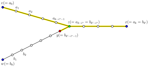
Figure 1: $a_{0},a_{1},\dots,a_{k}$ is a shortest $v$-to-$x$ path, and $b_{0},b_{1},\dots,b_{k^{\prime}}$ is a shortest $w$-to-$x$ path. The vertex $z$ represents the branching point of these two paths. Since the vertex $x$ is $v$-interesting, the highlighted edges are indispensable.

Let $y$ denote the vertex $b_{k^{\prime}-i^{*}-1}$. Since $y$ is on a shortest $w$-to-$x$ path, we have

$$\delta(w,x)=\delta(w,y)+\delta(y,x)=\delta(w,y)+(i^{*}+1)\geq\ell(y)+(i^{*}+1),$$ (1)

where the inequality follows from the definition of $\ell(y)$. It remains to analyze the value of $\ell(y)$.

The edge $(z,y)$ is incident to the vertex $z$ $(=a_{k-i^{*}})$, so is indispensable. Thus either $y$ is the predecessor of $z$, or $z$ is the predecessor of $y$. From the previous claim, $a_{k-i^{*}-1}$ is the predecessor of $z$. Since the predecessor of $z$ is unique (2) and $y\neq a_{k-i^{*}-1}$ (by definition of $i^{*}$), $y$ cannot be the predecessor of $z$, so $z$ is the predecessor of $y$. Again by 2, $\ell(y)=\ell(z)+1$. Since $\ell(z)=\ell(a_{k-i^{*}})=k-i^{*}$ by the previous claim, we have $\ell(y)=k-i^{*}+1$. We conclude from Equation 1 that

$$\delta(w,x)\geq(k-i^{*}+1)+(i^{*}+1)=k+2,$$

which implies that $x\in D(v,w)$.

We proved that $I_{k}(v)\subseteq D(v,w)$. Similarly, $I_{k}(w)\subseteq D(v,w)$. Therefore, $I_{k}(v)\cup I_{k}(w)\subseteq D(v,w)$.

We complete the proof of Lemma 3.5.

3.2.2 Proof of Lemma 3.6

To begin with, we show that there are relatively few dispensable edges within a neighborhood of $\{v,w\}$. This property, also called the locally tree-like property, was previously exploited by Bollobás [10] for three levels of neighborhoods on random $\Delta$-regular graphs in the context of automorphisms of those graphs. In Lemma 3.7, we extend the analysis from [10] to show the locally tree-like property for $M=\lceil\log\log n\rceil$ levels of neighborhoods.

Lemma 3.7.

Let $M=\lceil\log\log n\rceil$. We can construct two non-decreasing sequences $\{g_{i}\}_{1\leq i\leq M}$ and $\{L_{i}\}_{1\leq i\leq M}$, such that all of the following properties hold when $n$ is large enough:

1. $g_{1}=3$; and for any $i\in[2,M]$, $g_{i}=o\left((\Delta-1)^{L_{i-1}}/M\right)$;

2. $L_{M}\geq\lceil\log_{\Delta-1}(3n/\log n)\rceil+2$;

3. With probability $1-o(n^{-2})$, for all $i\in[1,M]$, strictly less than $g_{i}$ edges are dispensable among the edges incident to vertices in $U_{\leq L_{i}}$.

Proof 3.8 (Proof of Lemma 3.7).

First, we define two sequences $\{g_{i}\}_{1\leq i\leq M}$ and $\{f_{i}\}_{1\leq i\leq M}$ as follows: $g_{1}=3$, $f_{1}=\left\lceil n^{1/8}\right\rceil$, and for each $i\in[2,M]$, let

$$g_{i}=\left\lceil n^{1-7/2^{i+1}}/(\log n)^{1/2}\right\rceil,$$

$$f_{i}=\left\lceil n^{1-7/2^{i+2}}/(\log n)^{1/3}\right\rceil.$$

Next, we define the sequence $\{L_{i}\}_{1\leq i\leq M}$ as follows: for each $i\in[1,M]$, let

$$L_{i}=\left\lceil\log_{\Delta-1}f_{i}\right\rceil-6.$$

It is easy to see that all of the three sequences $\{g_{i}\}_{1\leq i\leq M}$, $\{f_{i}\}_{1\leq i\leq M}$, and $\{L_{i}\}_{1\leq i\leq M}$ are non-decreasing.

To show Property 1 of the statement, observe that for any $i\in[2,M]$,

$$g_{i}\cdot M=\left\lceil n^{1-7/2^{i+1}}/(\log n)^{1/2}\right\rceil\cdot\lceil\log\log n\rceil=o\left(n^{1-7/2^{i+1}}/(\log n)^{1/3}\right).$$

Thus $g_{i}\cdot M=o(f_{i-1})$ by definition of $f_{i-1}$. From the definition of $L_{i-1}$ and the fact that $\Delta=O(1)$, we have $f_{i-1}=\Theta\left((\Delta-1)^{L_{i-1}}\right)$. Therefore, $g_{i}\cdot M=o\left((\Delta-1)^{L_{i-1}}\right)$, hence $g_{i}=o\left((\Delta-1)^{L_{i-1}}/M\right)$.

To show Property 2 of the statement, observe that

$$f_{M}\geq n^{1-7/2^{(\log\log n)+2}}/(\log n)^{1/3}=2^{-7/4}\cdot n/(\log n)^{1/3}>(\Delta-1)^{8}\cdot 3n/\log n,$$

where the last inequality follows since $\Delta=O(1)$ and $n$ is large enough. Therefore, $L_{M}=\lceil\log_{\Delta-1}f_{M}\rceil-6\geq\lceil\log_{\Delta-1}(3n/\log n)\rceil+2$.

It remains to show Property 3 of the statement. Consider any integer $i\in[1,M]$. Since the graph is $\Delta$-regular, the number of vertices in $U_{\leq L_{i}}$ is at most

$$2+2\Delta\cdot\sum_{j=0}^{L_{i}-1}(\Delta-1)^{j}=2+\frac{2\Delta(\Delta-1)^{L_{i}}-2\Delta}{\Delta-2}<\frac{2\Delta(\Delta-1)^{L_{i}}}{\Delta-2}.$$

Let $n_{i}$ be the number of edges incident to vertices in $U_{\leq L_{i}}$. Since each vertex is incident to $\Delta$ edges, we have $n_{i}<\frac{2\Delta^{2}(\Delta-1)^{L_{i}}}{\Delta-2}$. Since $L_{i}=\left\lceil\log_{\Delta-1}f_{i}\right\rceil-6<\left(\log_{\Delta-1}f_{i}\right)-5$, we have $n_{i}<\frac{2\Delta^{2}}{(\Delta-2)(\Delta-1)^{5}}\cdot f_{i}$, which is less than $f_{i}$ since $\Delta\geq 3$.

In order to bound the number of dispensable edges incident to vertices in $U_{\leq L_{i}}$, it suffices to bound the number of dispensable edges among the first $f_{i}$ edges in the ordering of edge construction.

For any integer $t\in[1,\Delta n/2]$, denote $p(t)$ as the probability that the $t$-th edge in the construction is dispensable. We use the argument of Bollobás [10] to bound $p(t)$ as follows. Before constructing the $t$-th edge, the previously constructed $t-1$ edges are incident to at most $t+1$ vertices. For each of these $t+1$ vertices, at most $\Delta-1$ incident edges are not yet constructed. Thus $p(t)\leq\frac{(\Delta-1)(t+1)}{\Delta n-2(t-1)}$, which is less than $\frac{2t}{n}$ as soon as $t=o(n)$.

From the definition of $f_{i}$, we have $f_{i}\leq n/(\log n)^{1/3}=o(n)$, thus $p(f_{i})<\frac{2f_{i}}{n}$. The probability that there exist $g_{i}$ dispensable edges among the first $f_{i}$ edges is at most

$$\binom{f_{i}}{g_{i}}\cdot\left(\frac{2f_{i}}{n}\right)^{g_{i}}<\left(\frac{e\cdot f_{i}}{g_{i}}\right)^{g_{i}}\cdot\left(\frac{2f_{i}}{n}\right)^{g_{i}},$$

where the inequality follows from Stirling’s formula. When $i=1$, we have

$$\left(\frac{e\cdot f_{1}}{g_{1}}\right)^{g_{1}}\cdot\left(\frac{2f_{1}}{n}\right)^{g_{1}}=\left(\frac{2e\cdot\left(\lceil n^{1/8}\rceil\right)^{2}}{3n}\right)^{3}=o(n^{-17/8}),$$

and when $i\geq 2$, we have

$$\left(\frac{e\cdot f_{i}}{g_{i}}\right)^{g_{i}}\cdot\left(\frac{2f_{i}}{n}\right)^{g_{i}}=O\left(\left(\frac{2e}{(\log n)^{1/6}}\right)^{g_{i}}\right)=o(n^{-17/8}),$$

by definition of $g_{i}$ and $f_{i}$ and by observing that $g_{i}\geq n^{1/8}/(\log n)^{1/2}$ for any $i\geq 2$.

Thus for any $i\in[1,M]$, with probability $1-o(n^{-17/8})$, strictly less than $g_{i}$ edges are dispensable among the first $f_{i}$ edges, hence strictly less than $g_{i}$ edges are dispensable among the edges incident to vertices in $U_{\leq L_{i}}$.

Therefore, with probability $1-o(M\cdot n^{-17/8})=1-o(n^{-2})$, for all $i\in[1,M]$, strictly less than $g_{i}$ edges are dispensable among the edges incident to vertices in $U_{\leq L_{i}}$. This completes the proof for Property 3 of the statement.

We condition on the occurrence of the high probability event in Property 3 of Lemma 3.7. Let $\mathcal{E}$ denote this event.

We say that a dispensable edge is trivial if it is incident to $v$ or incident to $w$, and non-trivial otherwise. Let $E_{0}$ be the set of trivial dispensable edges. Let $E_{1}$ be the set of non-trivial dispensable edges that are incident to vertices in $U_{\leq L_{1}}$. The event $\mathcal{E}$ implies that strictly less than $g_{1}(=3)$ edges are dispensable among the edges incident to vertices in $U_{\leq L_{1}}$. Hence $|E_{0}|+|E_{1}|\leq 2$.

Let $F_{0}\subseteq U_{1}$ be the set of vertices $u\in U_{1}$ such that $u$ is not incident to any trivial dispensable edge. We claim that $|F_{0}|\geq 2\Delta-2|E_{0}|$. If $E_{0}=\emptyset$, it is clear that $|F_{0}|=2\Delta$. If $E_{0}\neq\emptyset$, there are three cases for each trivial dispensable edge in $E_{0}$: (1) a self-loop at $v$ or at $w$, (2) a parallel edge incident to $v$ or incident to $w$, and (3) an edge $(v,u)$ when $u$ is a neighbor of $w$, or an edge $(w,u)$ when $u$ is a neighbor of $v$. In all the three cases, the existence of each trivial dispensable edge in $E_{0}$ decreases the size of $F_{0}$ by at most 2. Hence $|F_{0}|\geq 2\Delta-2|E_{0}|$.

For each $u\in F_{0}$, define

$$T(u)=\{x\in U_{\leq L_{1}}\mid\ell(x)=\delta(x,u)+1\}.$$

Let $F\subseteq F_{0}$ be the set of vertices $u\in F_{0}$ such that $T(u)$ contains no vertex incident to a dispensable edge in $E_{1}$. Since each dispensable edge in $E_{1}$ is incident to two vertices, we have

$$|F|\geq|F_{0}|-2|E_{1}|\geq 2\Delta-2|E_{0}|-2|E_{1}|\geq 2(\Delta-2).$$

Since $F\subseteq F_{0}\subseteq U_{1}$, one of $v$ and $w$ has at least $|F|/2\geq\Delta-2$ neighbors in $F$.

Without loss of generality, we assume that $v$ has at least $\Delta-2$ neighbors in $F$. We show that, under this assumption, $|I_{k}(v)|\geq(\Delta-2-o(1))(\Delta-1)^{k-1}$.

Our proof proceeds in increasing order on $k\geq 1$.

First, consider any integer $k\in[1,L_{1}]$. Let $u$ be any neighbor of $v$ in $F$. Since $T(u)$ contains no vertex incident to a dispensable edge, $T(u)$ corresponds to a complete $(\Delta-1)$-ary tree. Consider any vertex $x\in T(u)$ such that $\delta(v,x)=k$. Any vertex $z\in V\setminus\{v\}$ such that $\delta(v,z)+\delta(z,x)=\delta(v,x)$ belongs to the (unique) shortest $x$-to-$u$ path. Since the shortest $x$-to-$u$ path is completely within $T(u)$, we have $z\in T(u)$, thus the edges incident to $z$ are indispensable. Hence $x$ is $v$-interesting according to Definition 3.4. Since $\delta(v,x)=k$, we have $x\in I_{k}(v)$. There are at least $\Delta-2$ choices of $u$, and for a fixed $u$, there are $(\Delta-1)^{k-1}$ choices of $x$. Therefore, the size of $I_{k}(v)$ is at least $(\Delta-2)(\Delta-1)^{k-1}$.

Next, consider any integer $k\in[L_{1}+1,L_{2}]$. For any vertex $x\in I_{L_{1}}(v)$, define

$$T^{\prime}(x)=\{y\in U_{\leq L_{2}}\mid\ell(y)=\delta(y,x)+L_{1}\}.$$

Let $F^{\prime}\subseteq I_{L_{1}}(v)$ be the set of vertices $x\in I_{L_{1}}(v)$ such that $T^{\prime}(x)$ contains no vertex incident to a dispensable edge. The event $\mathcal{E}$ implies that strictly less than $g_{2}$ dispensable edges are incident to vertices in $U_{\leq L_{2}}$. Since each dispensable edge is incident to two vertices, we have $|F^{\prime}|>|I_{L_{1}}(v)|-2g_{2}$. Let $x$ be any vertex in $F^{\prime}$. Since $T^{\prime}(x)$ contains no vertex incident to a dispensable edge, $T^{\prime}(x)$ corresponds to a complete $(\Delta-1)$-ary tree. Consider any vertex $y\in T^{\prime}(x)$ such that $\delta(v,y)=k$. Any vertex $z\in V\setminus\{v\}$ such that $\delta(v,z)+\delta(z,y)=\delta(v,y)$ belongs either to the (unique) shortest $x$-to-$v$ path or to the (unique) shortest $y$-to-$x$ path. In the first case, since $x$ is $v$-interesting, the edges incident to $z$ are indispensable by Definition 3.4. In the second case, since the shortest $y$-to-$x$ path is completely within $T^{\prime}(x)$, we have $z\in T^{\prime}(x)$, thus the edges incident to $z$ are indispensable. Hence $y$ is $v$-interesting according to Definition 3.4. Since $\delta(v,y)=k$, we have $y\in I_{k}(v)$. There are $|F^{\prime}|>|I_{L_{1}}(v)|-2g_{2}$ choices of $x$, and for a fixed $x$, there are $(\Delta-1)^{k-L_{1}}$ choices of $y$. Therefore,

$$|I_{k}(v)| >(|I_{L_{1}}(v)|-2g_{2})\cdot(\Delta-1)^{k-L_{1}}$$

$$\geq((\Delta-2)(\Delta-1)^{L_{1}-1}-2g_{2})\cdot(\Delta-1)^{k-L_{1}}$$

$$=(\Delta-2-o(1/M))(\Delta-1)^{k-1},$$

where the equality follows because $g_{2}=o((\Delta-1)^{L_{1}}/M)$ from Lemma 3.7 and since $\Delta=O(1)$.

We move on to larger values of $k$. Let $i$ be any integer in $[3,M]$. From Lemma 3.7, strictly less than $g_{i}$ edges are dispensable among the edges incident to vertices in $U_{\leq L_{i}}$ and that $g_{i}=o\left((\Delta-1)^{L_{i-1}}/M\right)$. For any integer $k\in[L_{i-1}+1,L_{i}]$, by extending the previous argument, we have

$$|I_{k}(v)|>(\Delta-2-i\cdot o(1/M))(\Delta-1)^{k-1}=(\Delta-2-o(1))(\Delta-1)^{k-1}.$$

We conclude that for any $k\in[1,L_{M}]$, we have $|I_{k}(v)|\geq(\Delta-2-o(1))(\Delta-1)^{k-1}$. In the other case that $w$ has at least $\Delta-2$ neighbors in $F$, similarly, we have $|I_{k}(w)|\geq(\Delta-2-o(1))(\Delta-1)^{k-1}.$ Hence $|I_{k}(v)\cup I_{k}(w)|\geq(\Delta-2-o(1))(\Delta-1)^{k-1}$. The event $\mathcal{E}$, on which the above analysis is conditioned, occurs with probability $1-o(n^{-2})$ according to Lemma 3.7. Therefore, with probability $1-o(n^{-2})$, we have

$$|I_{k}(v)\cup I_{k}(w)|\geq(\Delta-2-o(1))(\Delta-1)^{k-1},\text{ for any }k\in[1,L_{M}].$$

Again by Lemma 3.7, we have $L_{M}\geq\lceil\log_{\Delta-1}(3n/\log n)\rceil+2$. Thus the above inequality holds for any positive integer $k\leq\lceil\log_{\Delta-1}(3n/\log n)\rceil+2$.

We complete the proof of Lemma 3.6.

3.2.3 Proof of the Structural Lemma (Lemma 3.3) using Lemmas 3.5 and 3.6

We set $k=\lceil\log_{\Delta-1}(3n/\log n)\rceil+2$. By Lemma 3.5, $|D(v,w)|\geq|I_{k}(v)\cup I_{k}(w)|.$ By Lemma 3.6, with probability $1-o(n^{-2})$, we have

$$|I_{k}(v)\cup I_{k}(w)|>(\Delta-2-o(1))(\Delta-1)^{k-1}\geq(\Delta-2-o(1))(\Delta-1)\cdot(3n/\log n),$$

where the last inequality follows from the definition of $k$. Since $\Delta\geq 3$, we have $(\Delta-2-o(1))(\Delta-1)>1$. Thus with probability $1-o(n^{-2})$, we have $|I_{k}(v)\cup I_{k}(w)|>3n/\log n$, which implies that $|D(v,w)|>3n/\log n$.

We complete the proof of Lemma 3.3.

3.3 Proof of Lemma 3.1 using the Structural Lemma

Let $G$ be a random graph and let $S$ be a random subset of vertices, both defined in the statement of Lemma 3.1. According to Lemma 2.4, $\mathbb{E}_{G,S}\big{[}|\hat{E}\setminus E|\big{]}\leq\mathbb{E}_{G}\big{[}|B|\big{]}+o(1)$. It suffices to prove that $\mathbb{E}_{G}\big{[}|B|\big{]}=o(1)$.

First, we consider the case when $\Delta=O(1)$ is such that $\Delta\geq 3$. Our analysis is based on the configuration model. Let $G^{\prime}$ be a multigraph corresponding to a uniformly random configuration. Let $\mathbb{E}_{G^{\prime}}\big{[}|B|\big{]}$ denote the expected size of the set $B$ defined on $G^{\prime}$. Since each $\Delta$-regular graph corresponds to the same number of configurations and because the probability spaces of configurations and of $\Delta$-regular graphs, respectively, are uniform, we have $\mathbb{E}_{G}\big{[}|B|\big{]}\leq\mathbb{E}_{G^{\prime}}\big{[}|B|\big{]}/p$, where $p$ is the probability that $G^{\prime}$ is both simple and connected. According to [44], when $\Delta\geq 3$, $p\sim e^{(1-\Delta^{2})/4}$, which is constant since $\Delta=O(1)$. Thus $\mathbb{E}_{G}\big{[}|B|\big{]}=O(\mathbb{E}_{G^{\prime}}\big{[}|B|\big{]})$.

In order to bound $\mathbb{E}_{G^{\prime}}\big{[}|B|\big{]}$, consider any vertex pair $\{v,w\}$ in $G^{\prime}$ such that $\delta(v,w)\geq 2$. From the Structural Lemma (Lemma 3.3), the event $|D(v,w)|\leq 3n/\log n$ occurs with probability $o(n^{-2})$. Equivalently, the event $|D(v,w)|\leq 3n\cdot(\log n)/s$ occurs with probability $o(n^{-2})$, since $s=\log^{2}n$. Thus the event $\{v,w\}\in B$ occurs with probability $o(n^{-2})$ according to the definition of $B$ in Lemma 2.4. There are $n(n-1)/2$ vertex pairs $\{v,w\}$ in $G^{\prime}$. By linearity of expectation, $\mathbb{E}_{G^{\prime}}\big{[}|B|\big{]}$ is at most $o(n^{-2})\cdot n(n-1)/2=o(1)$. Hence $\mathbb{E}_{G}\big{[}|B|\big{]}=O(\mathbb{E}_{G^{\prime}}\big{[}|B|\big{]})=o(1)$.

In the special case when $\Delta=2$, a 2-regular graph $G$ is a ring. Consider any vertex pair $\{v,w\}$ in $G$ such that $\delta(v,w)\geq 2$. It is easy to see that at least $n-4$ vertices $u$ in the ring $G$ are such that $|\delta(u,v)-\delta(u,w)|>1$, so $|D(v,w)|\geq n-4$ by Definition 2.1. When $n$ is large enough, $n-4>3n/\log n$, so $|D(v,w)|>3n/\log n$. Equivalently, we have $|D(v,w)|>3n\cdot(\log n)/s$, since $s=\log^{2}n$. Thus $\{v,w\}\notin B$ according to the definition of $B$ in Lemma 2.4. Therefore, $B=\emptyset$ and $\mathbb{E}_{G}\big{[}|B|\big{]}=0$.

We conclude that $\mathbb{E}_{G}\big{[}|B|\big{]}=o(1)$ for any $\Delta=O(1)$. Thus $\mathbb{E}_{G,S}\big{[}|\hat{E}\setminus E|\big{]}\leq\mathbb{E}_{G}\big{[}|B|\big{]}+o(1)=o(1)$.

We complete the proof of Lemma 3.1.

Remark 3.9.

With more care in the construction of the sequences in Lemma 3.7, we can improve the bound in Property 2 of Lemma 3.7 by

$$L_{M}\geq\lceil\log_{\Delta-1}(3n/(\log\log n)^{2+\epsilon})\rceil+2,$$

for any $\epsilon>0$. As a result, the range of $k$ in Lemma 3.6 can be extended to $k\leq\lceil\log_{\Delta-1}(3n/(\log\log n)^{2+\epsilon})\rceil+2$, and consequently, the event in Lemma 3.3 can be replaced by $|D(v,w)|>3n/(\log\log n)^{2+\epsilon}$. Therefore, Lemma 3.1 holds for $s=\log n\cdot(\log\log n)^{2+\epsilon}$. This implies that the parameter $s$ in Theorem 1.1 can be reduced to $\log n\cdot(\log\log n)^{2+\epsilon}$.

4 Other Reconstruction Models (Proofs of Corollaries 1.3, 1.2 and 1.4)

In this section, we study the reconstruction of random $\Delta$-regular graphs in the all-distances query model, in the betweenness query model, as well as in the parallel setting.

By extending the analysis from Section 3, we observe that the set $\hat{E}$ constructed in Simple (Algorithm 1) equals the edge set $E$ with high probability, in Lemma 4.1.

Lemma 4.1.

Let $G$ be a uniformly random $\Delta$-regular graph with $\Delta=O(1)$. Let $s=\log^{2}n$. Let $S\subseteq V$ be a set of $s$ vertices selected uniformly and independently at random from $V$. With probability $1-o(1)$, $|\hat{E}|=\Delta n/2$. In addition, the event $|\hat{E}|=\Delta n/2$ implies $\hat{E}=E$.

Proof 4.2.

From Lemma 3.1, $\mathbb{E}_{G,S}\big{[}|\hat{E}\setminus E|\big{]}=o(1)$. By Markov’s inequality, the event that $|\hat{E}\setminus E|\geq 1$ occurs with probability $o(1)$. Thus with probability $1-o(1)$, we have $\hat{E}\subseteq E$. On the other hand, $E\subseteq\hat{E}$ by 1. Therefore, the event that $\hat{E}=E$ occurs with probability $1-o(1)$, and this event occurs if and only if $|\hat{E}|=|E|$. The statement follows since $|E|=\Delta n/2$ in a $\Delta$-regular graph.

4.1 A Modified Algorithm

Lemma 4.1 enables us to design another reconstruction algorithm in the distance query model, called Simple-Modified, which is a modified version of Simple, see Algorithm 2. Simple-Modified repeatedly computes a set $\hat{E}$ as in Simple, until the size of $\hat{E}$ equals $\Delta n/2$. The parameter $s$ is fixed to $\log^{2}n$.

Algorithm 2 Simple-Modified $(V)$

1:repeat

2:     $S\leftarrow$ sample of $s=\log^{2}n$ vertices selected uniformly and independently at random from $V$

3:     for $u\in S$ and $v\in V$ do Query$(u,v)$      

4:     $\hat{E}\leftarrow$ set of vertex pairs $\{a,b\}\subseteq V$ such that, for all $u\in S$, $|\delta(u,a)-\delta(u,b)|\leq 1$

5:until $|\hat{E}|=\Delta n/2$

6:return $\hat{E}$

Lemma 4.3.

Let $G$ be a uniformly random $\Delta$-regular graph with $\Delta=O(1)$. In the distance query model, Simple-Modified (Algorithm 2) is a reconstruction algorithm, i.e., its output equals the edge set $E$. The expected number of iterations of the repeat loop in Simple-Modified is $1+o(1)$.

Proof 4.4.

Upon termination of the repeat loop in Simple-Modified, we have $|\hat{E}|=\Delta n/2$, which implies $\hat{E}=E$ by Lemma 4.1. Thus the output of Simple-Modified equals the edge set $E$.

In each iteration of the repeat loop, the event that $|\hat{E}|=\Delta n/2$ occurs with probability $1-o(1)$ by Lemma 4.1. Thus the expected number of iterations of the repeat loop is $1+o(1)$.

4.2 All-Distances Query Model (Proof of Corollary 1.2)

By Lemma 4.3, Simple-Modified is a reconstruction algorithm in the distance query model. We extend Simple-Modified to the all-distances query model.

Observe that in Simple-Modified, the distance queries are performed between each sampled vertex $u\in S$ and all vertices in the graph. This is equivalent to a single query at each sampled vertex $u\in S$ in the all-distances query model. Hence each iteration of the repeat loop in Simple-Modified corresponds to $|S|=\log^{2}n$ all-distances queries. Again by Lemma 4.3, the expected number of iterations of the repeat loop in Simple-Modified is $1+o(1)$. Therefore, in the all-distances query model, an algorithm equivalent to Simple-Modified reconstructs the graph using $(1+o(1))\cdot\log^{2}n=O(\log^{2}n)$ all-distances queries in expectation.

4.3 Betweenness Query Model (Proof of Corollary 1.3)

In the betweenness query model, Abrahamsen et al. [1] showed that $\tilde{O}(\Delta^{2}\cdot n)$ betweenness queries suffice to compute the distances from a given vertex to all vertices in the graph (it is implicit in Lemma 16 from [1]), so an all-distances query can be simulated by $\tilde{O}(\Delta^{2}\cdot n)$ betweenness queries. As a consequence of Corollary 1.2, we achieve a reconstruction algorithm using $\tilde{O}(\Delta^{2}\cdot n\cdot\log^{2}n)=\tilde{O}(n)$ betweenness queries in expectation, since $\Delta=O(1)$.

4.4 Parallel Setting (Proof of Corollary 1.4)

By Lemma 4.3, Simple-Modified is a reconstruction algorithm in the distance query model. We analyze Simple-Modified in the parallel setting.

Each iteration of the repeat loop consists of $n\cdot\log^{2}n$ distance queries, and the distance queries within the same iteration of the repeat loop can be performed in parallel. Again by Lemma 4.3, the expected number of iterations of the repeat loop in Simple-Modified is $1+o(1)$. Thus the expected number of rounds in Simple-Modified is $1+o(1)$, and the expected number of distance queries in Simple-Modified is $(1+o(1))\cdot n\cdot\log^{2}n=\tilde{O}(n)$.

5 Metric Dimension (Proof of Corollary 1.5)

In this section, we study the metric dimension of random $\Delta$-regular graphs. To begin with, we show an elementary structural property of random $\Delta$-regular graphs, in Lemma 5.1, based on a classical result on those graphs.

Lemma 5.1.

Let $G=(V,E)$ be a uniformly random $\Delta$-regular graph with $\Delta=O(1)$. With probability $1-o(1)$, for any edge $(a,b)$ of the graph $G$, there exists a vertex $c\in V\setminus\{a,b\}$ that is adjacent to $b$ but is not adjacent to $a$.

Proof 5.2.

First, consider the case when $\Delta=2$. A $2$-regular graph is a ring. Let $(a,b)$ be any edge of the graph. The vertex $b$ has two neighbors, the vertex $a$ and another vertex, let it be $c$. We have $c\in V\setminus\{a,b\}$ and $c$ is not adjacent to $a$ (as soon as $n>3$). The statement of the lemma follows.

Next, consider the case when $\Delta=O(1)$ is such that $\Delta\geq 3$. Let $\mathcal{E}$ denote the event that, for any edge $(a,b)$ of $G$, there do not exist two vertices $c_{1}$ and $c_{2}$ in $G$, such that all of the 4 edges $(a,c_{1}),(a,c_{2}),(b,c_{1}),(b,c_{2})$ belong to $G$. We show that $\mathcal{E}$ occurs with probability $1-o(1)$. Indeed, if for some edge $(a,b)$ of $G$, there exist two vertices $c_{1}$ and $c_{2}$ such that $(a,c_{1}),(a,c_{2}),(b,c_{1}),(b,c_{2})$ are edges of $G$, then the induced subgraph on $\{a,b,c_{1},c_{2}\}$ consists of at least 5 edges. A classical result on random $\Delta$-regular graphs shows that, for any constant integer $k$, the probability that there exists an induced subgraph of $k$ vertices with at least $k+1$ edges is $o(1)$, see, e.g., Lemma 11.12 in [18]. Therefore, $\mathcal{E}$ occurs with probability $1-o(1)$.

We condition on the occurrence of $\mathcal{E}$. For any edge $(a,b)$ of $G$, let $N(a)$ be the set of $\Delta-1$ neighbors of $a$ that are different from $b$, and let $N(b)$ be the set of $\Delta-1$ neighbors of $b$ that are different from $a$. Since $\Delta\geq 3$, we have $|N(a)|=|N(b)|\geq 2$. The event $\mathcal{E}$ implies that $N(a)\neq N(b)$, so there exists a vertex $c\in N(b)\setminus N(a)$. By definition, $c$ is adjacent to $b$ but is not adjacent to $a$, and $c\in V\setminus\{a,b\}$. Since $\mathcal{E}$ occurs with probability $1-o(1)$, we conclude that, with probability $1-o(1)$, for any edge $(a,b)$ of the graph $G$, there exists a vertex $c\in V\setminus\{a,b\}$ that is adjacent to $b$ but is not adjacent to $a$.

Definition 5.3 (e.g., [5, 13]).

A subset of vertices $S\subseteq V$ is a resolving set for a graph $G=(V,E)$ if, for any pair of vertices $\{a,b\}\subseteq V$, there is a vertex $u\in S$ such that $\delta(u,a)\neq\delta(u,b)$. The metric dimension of $G$ is the smallest size of a resolving set for $G$.

Based on the analysis of Simple from Lemma 4.1 and the structural property from Lemma 5.1, we show that, with high probability, a random subset of $\log^{2}n$ vertices is a resolving set for a random $\Delta$-regular graph, in Lemma 5.4.

Lemma 5.4.

Let $G=(V,E)$ be a uniformly random $\Delta$-regular graph with $\Delta=O(1)$. Let $S\subseteq V$ be a sample of $s=\log^{2}n$ vertices selected uniformly and independently at random from $V$. With probability $1-o(1)$, the set $S$ is a resolving set for the graph $G$.

Proof 5.5.

Let $\mathcal{E}_{1}$ denote the event that, for any edge $(a,b)$ of the graph $G$, there exists a vertex $c\in V\setminus\{a,b\}$ that is adjacent to $b$ but is not adjacent to $a$. By Lemma 5.1, the event $\mathcal{E}_{1}$ occurs with probability $1-o(1)$. Let $\mathcal{E}_{2}$ denote the event $\hat{E}=E$. By Lemma 4.1, the event $\mathcal{E}_{2}$ occurs with probability $1-o(1)$. Thus with probability $1-o(1)$, both events $\mathcal{E}_{1}$ and $\mathcal{E}_{2}$ occur simultaneously. We condition on the occurrences of both events $\mathcal{E}_{1}$ and $\mathcal{E}_{2}$ in the subsequent analysis.

First, consider any vertex pair $\{a,b\}\subseteq V$ such that $\delta(a,b)\geq 2$. The event $\mathcal{E}_{2}$ implies that $\{a,b\}\notin\hat{E}$. By definition, there exists some vertex $u\in S$ such that $|\delta(u,a)-\delta(u,b)|\geq 2$, which implies that $\delta(u,a)\neq\delta(u,b)$.

Next, consider any vertex pair $\{a,b\}\subseteq V$ such that $\delta(a,b)=1$. The event $\mathcal{E}_{1}$ implies that there exists a vertex $c\in V\setminus\{a,b\}$ that is adjacent to $b$ but is not adjacent to $a$. Since $\delta(a,c)\geq 2$, the event $\mathcal{E}_{2}$ implies that $\{a,c\}\notin\hat{E}$. By definition, there exists some vertex $u\in S$ such that $|\delta(u,a)-\delta(u,c)|\geq 2$. Using an elementary inequality of $|x-y|+|y-z|\geq|x-z|$ for any three real numbers $x$, $y$, and $z$, we have

$$|\delta(u,a)-\delta(u,b)| \geq|\delta(u,a)-\delta(u,c)|-|\delta(u,b)-\delta(u,c)|$$

$$\geq|\delta(u,a)-\delta(u,c)|-\delta(b,c)$$ (by triangle inequality)

$$\geq 2-\delta(b,c) u$$ (by definition of )

$$\geq 1 (b,c)$$ (since is an edge) .

Thus $\delta(u,a)\neq\delta(u,b)$.

Therefore, conditioned on the occurrences of both events $\mathcal{E}_{1}$ and $\mathcal{E}_{2}$, for any vertex pair $\{a,b\}\subseteq V$, there exists a vertex $u\in S$ such that $\delta(u,a)\neq\delta(u,b)$.

We conclude that, with probability $1-o(1)$, the set $S$ is a resolving set for $G$.

From Lemma 5.4, with probability $1-o(1)$, the metric dimension of a random $\Delta$-regular graph is at most $\log^{2}n$. This completes the proof of Corollary 1.5.

6 Reconstruction of Bounded-Degree Graphs (Proof of Theorem 1.6)

In this section, we analyze Simple (Algorithm 1) on general graphs of bounded degree in the distance query model. Recall that a set $B$ of vertex pairs $\{a,b\}\subseteq V$ is defined in Lemma 2.4. For every vertex $a\in V$, we define the set of vertices $B(a)\subseteq V$ as

$$B(a)=\big{\{}b\in V\mid\{a,b\}\in B\big{\}}.$$

Intuitively, $B(a)$ consists of the vertices $b\in V$ that has few distinguishers with $a$. We bound the size of the set $B(a)$ for any vertex $a$, in Lemma 6.1.

Lemma 6.1.

Let $G$ be a general graph of bounded degree $\Delta$. For any vertex $a\in V$, $|B(a)|\leq 9\Delta^{3}\cdot n^{2}\cdot(\log^{2}n)/s^{2}$.

We defer the proof of Lemma 6.1 for the moment and first show how it implies Theorem 1.6.

Proof 6.2 (Proof of Theorem 1.6 using Lemma 6.1).

By Lemma 2.2, Simple is a reconstruction algorithm using $n\cdot s+|\hat{E}|$ distance queries, and in addition, Simple can be parallelized using 2 rounds. It remains to further analyze the query complexity.

From 1, $|\hat{E}|=|E|+|\hat{E}\setminus E|$. Since the graph has bounded degree $\Delta$, $|E|\leq\Delta n$. From Lemma 2.4, $\mathbb{E}_{S}\big{[}|\hat{E}\setminus E|\big{]}\leq|B|+o(1)$. Therefore, the expected number of distance queries in Simple is at most $n\cdot s+\Delta n+|B|+o(1)$. It suffices to analyze $|B|$.

Observe that $|B|\leq\sum_{a\in V}|B(a)|$ by definition of $\{B(a)\}_{a\in V}$. From Lemma 6.1, $|B(a)|\leq 9\Delta^{3}\cdot n^{2}\cdot(\log^{2}n)/s^{2}$, for any vertex $a\in V$. Hence $|B|\leq(9\Delta^{3}\cdot n^{2}\cdot(\log^{2}n)/s^{2})\cdot n$. Thus the expected number of distance queries in Simple is at most $n\cdot s+\Delta n+(9\Delta^{3}\cdot n^{2}\cdot(\log^{2}n)/s^{2})\cdot n+o(1)$, which is $\tilde{O}(n^{5/3})$ since $s=n^{2/3}$ and $\Delta=O(\operatorname{polylog}n)$.

The rest of the section is dedicated to prove Lemma 6.1.

Let $a$ be any vertex in $V$. Let $T$ be an (arbitrary) shortest-path tree rooted at $a$ and spanning all vertices in $V$. For any vertex $b\in V$, let the shortest $a$-to-$b$ path denote the path between $a$ and $b$ in the tree $T$. To simplify the presentation, we assume that, for any $b\in B(a)$, $\delta(a,b)$ is even, so that the midpoint vertex of the shortest $a$-to-$b$ path is uniquely defined. We extend our analysis to the general setting in the end of the section.

For any vertex $m\in V$, define the set $B(a,m)\subseteq B(a)$ as

$$B(a,m)=\big{\{}b\in B(a)\mid\text{the midpoint vertex of the shortest $a$-to-$b$ path is $m$}\big{\}}.$$

Define the set $M(a)\subseteq V$ as

$$M(a)=\big{\{}m\in V\mid B(a,m)\neq\emptyset\big{\}}.$$

In other words, $M(a)$ consists of the vertices $m\in V$ that is the midpoint vertex of the shortest $a$-to-$b$ path for some $b\in B(a)$. From the construction, we have

$$B(a)=\bigcup_{m\in M(a)}B(a,m).$$ (2)

In order to bound the size of $B(a)$, first we bound the size of $B(a,m)$ for any midpoint $m\in M(a)$, in Lemma 6.3, and then we bound the number of distinct midpoints, in Lemma 6.5.

Lemma 6.3.

For any $m\in M(a)$, $|B(a,m)|\leq 3\Delta\cdot n\cdot(\log n)/s$.

Proof 6.4.

For any $b\in B(a,m)$, the vertex $m$ is the midpoint vertex of the shortest $a$-to-$b$ path by definition. From the assumption, $\delta(a,b)$ is even for any $b\in B(a,m)$, so there exists for some positive integer $\ell$, such that $\delta(m,a)=\ell$ and $\delta(m,b)=\ell$ for any $b\in B(a,m)$.

For every neighbor $m^{\prime}$ of $m$ such that $\delta(a,m^{\prime})=\delta(a,m)+1$, define a set $Y(m^{\prime})\subseteq B(a,m)$ that consists of the vertices $b\in B(a,m)$ such that $m^{\prime}$ is on the shortest $a$-to-$b$ path. Let $\hat{m}$ be a neighbor of $m$ such that $\delta(a,\hat{m})=\delta(a,m)+1$ and that $|Y(\hat{m})|$ is maximized, see Figure 2. Since the graph has bounded degree $\Delta$, we have $|B(a,m)|\leq\Delta\cdot|Y(\hat{m})|$. It suffices to bound $|Y(\hat{m})|$.

The main observation is that any vertex of $Y(\hat{m})$ distinguishes $a$ and any other vertex of $Y(\hat{m})$. To see this, let $b_{0}$ be any vertex in $Y(\hat{m})$. By definition, $\delta(a,\hat{m})=\delta(a,m)+1=\ell+1$. Since $\hat{m}$ is on the shortest $a$-to-$b_{0}$ path, we have $\delta(\hat{m},b_{0})=\delta(a,b_{0})-\delta(a,\hat{m})=\ell-1$, thus $\delta(\hat{m},b_{0})=\delta(\hat{m},a)-2$. For any vertex $b_{1}\in Y(\hat{m})$, from the triangle inequalities on $\delta$, we have

$$\delta(b_{1},b_{0})\leq\delta(b_{1},\hat{m})+\delta(\hat{m},b_{0})=\delta(b_{1},\hat{m})+\delta(\hat{m},a)-2=\delta(b_{1},a)-2.$$

According to Definition 2.1, the vertex $b_{1}$ distinguishes $a$ and $b_{0}$, and equivalently, $b_{1}\in D(a,b_{0})$. Thus we have $Y(\hat{m})\subseteq D(a,b_{0})$, hence $|Y(\hat{m})|\leq|D(a,b_{0})|\leq 3n\cdot(\log n)/s$ using the fact that $b_{0}\in Y(\hat{m})\subseteq B(a)$ and the definition of $B$ in Lemma 2.4.

We conclude that $|B(a,m)|\leq\Delta\cdot|Y(\hat{m})|\leq 3\Delta\cdot n\cdot(\log n)/s.$

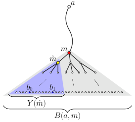
Figure 2: The vertex $m$ is the midpoint of the shortest path between $a$ and any vertex in $B(a,m)$. The vertex $\hat{m}$ is a well-chosen neighbor of $m$. Consider any vertex $b_{0}\in Y(\hat{m})$. We can show that any vertex $b_{1}\in Y(\hat{m})$ distinguishes $a$ and $b_{0}$.

Lemma 6.5.

$|M(a)|\leq 3\Delta\cdot n\cdot(\log n)/s$.

Proof 6.6.

For each vertex $m\in M(a)$, denote $x_{m}$ as the second-to-last vertex on the shortest $a$-to-$m$ path. Denote $X(a)\subseteq V$ as the set of vertices $x_{m}$ for all $m\in M(a)$. See Figure 3. Since $G$ has bounded degree $\Delta$, we have $|M(a)|\leq\Delta\cdot|X(a)|$. It suffices to bound $|X(a)|$.

Let $b^{*}$ be a vertex in $B(a)$ such that $\delta(a,b^{*})$ is maximized. From the assumption, $\delta(a,b^{*})$ is even, so we denote $\delta(a,b^{*})=2\ell$ for some positive integer $\ell$.

The main observation is that any vertex of $X(a)$ distinguishes $a$ and $b^{*}$. To see this, let $x$ be any vertex in $X(a)$. Let $m$ be any vertex in $M(a)$ such that $x$ is the second-to-last vertex on the shortest $a$-to-$m$ path. We have $\delta(a,m)\leq\ell$ and $\delta(a,x)=\delta(a,m)-1\leq\ell-1.$ By the triangle inequality on the distances, $\delta(b^{*},x)\geq\delta(a,b^{*})-\delta(a,x)\geq 2\ell-(\ell-1)=\ell+1$. Thus $\delta(b^{*},x)-\delta(a,x)\geq 2$. According to Definition 2.1, the vertex $x$ distinguishes $a$ and $b^{*}$, and equivalently, $x\in D(a,b^{*})$. Thus $X(a)\subseteq D(a,b^{*})$, hence $|X(a)|\leq|D(a,b^{*})|\leq 3n\cdot(\log n)/s$ using the fact that $b^{*}\in B(a)$ and the definition of $B$ in Lemma 2.4.

We conclude that $|M(a)|\leq\Delta\cdot|X(a)|\leq 3\Delta\cdot n\cdot(\log n)/s.$

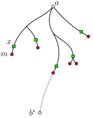
Figure 3: Solid circular nodes represent the vertices $m\in M(a)$. Solid curves represent the shortest $a$-to-$m$ paths. Solid square nodes represent the vertices in $X(a)$. Denote $b^{*}$ as a vertex in $B(a)$ that is farthest from $a$. We can show that any vertex $x\in X(a)$ distinguishes $a$ and $b^{*}$.

From Equation 2, $|B(a)|\leq\sum_{m\in M(a)}|B(a,m)|$. From Lemma 6.3, $|B(a,m)|\leq 3\Delta\cdot n\cdot(\log n)/s$ for every $m\in M(a)$. From Lemma 6.5, $|M(a)|\leq 3\Delta\cdot n\cdot(\log n)/s$. Therefore, $|B(a)|\leq 9\Delta^{2}\cdot n^{2}\cdot(\log^{2}n)/s^{2}$.

Finally, consider the general setting in which $\delta(a,b)$ is not necessarily even for any $b\in B(a)$. For a vertex $m$ on the shortest $a$-to-$b$ path, we say that $m$ is the midpoint vertex of that path if $\delta(a,m)=\lfloor\delta(a,b)/2\rfloor$. The definitions of $B(a,m)$ and $M(a)$ remain the same. Lemma 6.5 holds in the same way. In Lemma 6.3, the upper bound of $|B(a,m)|$ is replaced by $3\Delta^{2}\cdot n\cdot(\log n)/s$. Indeed, to extend the proof of Lemma 6.3, instead of considering vertex $m^{\prime}$ (resp., vertex $\hat{m}$) that is a neighbor of $m$, we consider $m^{\prime}$ (resp., $\hat{m}$) that is at distance 2 from $m$. We have $|B(a,m)|\leq\Delta^{2}\cdot|Y(\hat{m})|$. The bound $|Y(\hat{m})|\leq 3n\cdot(\log n)/s$ remains the same, so we have $|B(a,m)|\leq 3\Delta^{2}\cdot n\cdot(\log n)/s.$ Hence $|B(a)|\leq 9\Delta^{3}\cdot n^{2}\cdot(\log^{2}n)/s^{2}$.

We complete the proof of Lemma 6.1. Therefore, we obtain Theorem 1.6.

References

- [1] Mikkel Abrahamsen, Greg Bodwin, Eva Rotenberg, and Morten Stöckel. Graph Reconstruction with a Betweenness Oracle. In Symposium on Theoretical Aspects of Computer Science, pages 5:1–5:14. Schloss Dagstuhl–Leibniz-Zentrum fuer Informatik, 2016.
- [2] Dimitris Achlioptas, Aaron Clauset, David Kempe, and Cristopher Moore. On the bias of traceroute sampling: Or, power-law degree distributions in regular graphs. Journal of the ACM, 56(4):21:1–21:28, 2009.
- [3] Ramtin Afshar, Michael T. Goodrich, Pedro Matias, and Martha C. Osegueda. Reconstructing biological and digital phylogenetic trees in parallel. In European Symposium on Algorithms, volume 173, pages 3:1–3:24. Schloss Dagstuhl–Leibniz-Zentrum für Informatik, 2020.
- [4] Animashree Anandkumar, Avinatan Hassidim, and Jonathan Kelner. Topology discovery of sparse random graphs with few participants. Random Structures & Algorithms, 43(1):16–48, 2013.
- [5] Robert F. Bailey and Peter J. Cameron. Base size, metric dimension and other invariants of groups and graphs. Bulletin of the London Mathematical Society, 43(2):209–242, 2011.
- [6] Albert-László Barabási and Réka Albert. Emergence of scaling in random networks. science, 286(5439):509–512, 1999.
- [7] Zuzana Beerliova, Felix Eberhard, Thomas Erlebach, Alexander Hall, Michael Hoffmann, Matús Mihal’ak, and L. Shankar Ram. Network discovery and verification. IEEE Journal on Selected Areas in Communications, 24(12):2168–2181, 2006.
- [8] Vincent D. Blondel, Jean-Loup Guillaume, Julien M. Hendrickx, and Raphaël M. Jungers. Distance distribution in random graphs and application to network exploration. Physical Review E, 76(6):066101, 2007.
- [9] Béla Bollobás. A probabilistic proof of an asymptotic formula for the number of labelled regular graphs. European Journal of Combinatorics, 1(4):311–316, 1980.
- [10] Béla Bollobás. Distinguishing vertices of random graphs. North-Holland Mathematics Studies, 62:33–49, 1982.
- [11] Béla Bollobás, Dieter Mitsche, and Paweł Prałat. Metric dimension for random graphs. The Electronic Journal of Combinatorics, 20(4):P1, 2013.
- [12] José Cáceres, Carmen Hernando, Mercè Mora, Ignacio M. Pelayo, María L. Puertas, Carlos Seara, and David R. Wood. On the metric dimension of cartesian products of graphs. SIAM Journal on Discrete Mathematics, 21(2):423–441, 2007.
- [13] Gary Chartrand, Linda Eroh, Mark A. Johnson, and Ortrud R. Oellermann. Resolvability in graphs and the metric dimension of a graph. Discrete Applied Mathematics, 105(1-3):99–113, 2000.
- [14] Thomas Erlebach, Alexander Hall, Michael Hoffmann, and Matúš Mihal’ák. Network discovery and verification with distance queries. Algorithms and Complexity, pages 69–80, 2006.
- [15] Thomas Erlebach, Alexander Hall, and Matúš Mihal’ák. Approximate discovery of random graphs. In International Symposium on Stochastic Algorithms, pages 82–92. Springer, 2007.
- [16] Michalis Faloutsos, Petros Faloutsos, and Christos Faloutsos. On power-law relationships of the internet topology. ACM SIGCOMM, 29(4):251–262, 1999.
- [17] Florent Foucaud and Guillem Perarnau. Bounds for identifying codes in terms of degree parameters. Electronic Journal of Combinatorics, 19(P32), 2012.
- [18] Alan Frieze and Michał Karoński. Introduction to random graphs. https://www.math.cmu.edu/~af1p/BOOK.pdf.
- [19] Alan Frieze, Ryan Martin, Julien Moncel, Miklós Ruszinkó, and Cliff Smyth. Codes identifying sets of vertices in random networks. Discrete Mathematics, 307(9):1094–1107, 2007.
- [20] Jean-Loup Guillaume and Matthieu Latapy. Complex network metrology. Complex systems, 16(1):83, 2005.
- [21] Frank Harary and Robert A. Melter. On the metric dimension of a graph. Ars Combinatoria, 2(191-195), 1976.
- [22] Jotun J. Hein. An optimal algorithm to reconstruct trees from additive distance data. Bulletin of Mathematical Biology, 51(5):597–603, 1989.
- [23] Carmen Hernando, Merce Mora, Ignacio M. Pelayo, Carlos Seara, and David R. Wood. Extremal graph theory for metric dimension and diameter. Electronic Notes in Discrete Mathematics, 29:339–343, 2007. European Conference on Combinatorics, Graph Theory and Applications.
- [24] Imran Javaid, M. Tariq Rahim, and Kashif Ali. Families of regular graphs with constant metric dimension. Utilitas mathematica, 75:21–34, 2008.
- [25] Mihajlo Jovanović, Fred Annexstein, and Kenneth Berman. Modeling peer-to-peer network topologies through small-world models and power laws. In IX Telecommunications Forum, TELFOR, pages 1–4. Citeseer, 2001.
- [26] Sampath Kannan, Eugene L. Lawler, and Tandy Warnow. Determining the evolutionary tree using experiments. Journal of Algorithms, 21(1):26 – 50, 1996.
- [27] Sampath Kannan, Claire Mathieu, and Hang Zhou. Graph reconstruction and verification. ACM Transactions on Algorithms, 14(4):1–30, 2018.
- [28] Mark G. Karpovsky, Krishnendu Chakrabarty, and Lev B. Levitin. On a new class of codes for identifying vertices in graphs. IEEE Transactions on Information Theory, 44(2):599–611, 1998.
- [29] Samir Khuller, Balaji Raghavachari, and Azriel Rosenfeld. Landmarks in graphs. Discrete applied mathematics, 70(3):217–229, 1996.
- [30] Valerie King, Li Zhang, and Yunhong Zhou. On the complexity of distance-based evolutionary tree reconstruction. In Symposium on Discrete Algorithms, pages 444–453. SIAM, 2003.
- [31] Anukool Lakhina, John W. Byers, Mark Crovella, and Peng Xie. Sampling biases in IP topology measurements. In Twenty-second Annual Joint Conference of the IEEE Computer and Communications Societies, volume 1, pages 332–341. IEEE, 2003.
- [32] Dieter Mitsche and Juanjo Rué. On the limiting distribution of the metric dimension for random forests. European Journal of Combinatorics, 49:68–89, 2015.
- [33] Elchanan Mossel and Jiaming Xu. Seeded graph matching via large neighborhood statistics. Random Structures & Algorithms, 57(3):570–611, 2020.
- [34] Mark E. J. Newman, Duncan J. Watts, and Steven H. Strogatz. Random graph models of social networks. Proceedings of the national academy of sciences, 99(suppl 1):2566–2572, 2002.
- [35] Gergely Odor and Patrick Thiran. Sequential metric dimension for random graphs, 2020. arXiv:1910.10116.
- [36] Ortrud R. Oellermann and Joel Peters-Fransen. The strong metric dimension of graphs and digraphs. Discrete Applied Mathematics, 155(3):356–364, 2007.
- [37] Yunior Ramírez-Cruz, Ortrud R. Oellermann, and Juan A. Rodríguez-Velázquez. The simultaneous metric dimension of graph families. Discrete Applied Mathematics, 198:241–250, 2016.
- [38] Lev Reyzin and Nikhil Srivastava. Learning and verifying graphs using queries with a focus on edge counting. In Algorithmic Learning Theory, pages 285–297. Springer, 2007.
- [39] Guozhen Rong, Wenjun Li, Yongjie Yang, and Jianxin Wang. Reconstruction and verification of chordal graphs with a distance oracle. Theoretical Computer Science, 859:48–56, 2021.
- [40] András Sebő and Eric Tannier. On metric generators of graphs. Mathematics of Operations Research, 29(2):383–393, 2004.
- [41] Sandeep Sen and V. N. Muralidhara. The covert set-cover problem with application to network discovery. In WALCOM, pages 228–239. Springer, 2010.
- [42] Peter J. Slater. Leaves of trees. In Southeastern Conference on Combinatorics, Graph Theory, and Computing, pages 549–559, 1975.
- [43] Michael S. Waterman, Temple F. Smith, M. Singh, and W. A. Beyer. Additive evolutionary trees. Journal of Theoretical Biology, 64(2):199–213, 1977.
- [44] Nicholas C. Wormald. Models of random regular graphs. London Mathematical Society Lecture Note Series, pages 239–298, 1999.