Classification of
spin-chain braid representations

Abstract.

A braid representation is a monoidal functor from the braid category ${\mathsf{B}}$, for example given by a solution to the constant Yang-Baxter equation. Given a monoidal category $\mathsf{C}$ with $ob(\mathsf{C})={\mathbb{N}}$, a rank-$N$ charge-conserving representation, or spin-chain representation, is a strict monoidal functor $F$ from $\mathsf{C}$ to the category ${\mathsf{Match}}^{N}$ of rank-$N$ charge-conserving matrices (see below for definition), that is natural in the sense that $F(1)=1$. In this work we construct all spin-chain braid representations, and classify up to suitable notions of isomorphism.

1. Introduction

Classification of braid representations [Bir75] is a major open problem — except that it is impossibly wild. For applications, as we will discuss below, conceding this impossibility is not an acceptable outcome. So we seek a framework for a paradigm change. Clues for this can be found, for example, in higher representation theory (works such as [MM14, RW18, KV94, DMR20] and many others); and in higher lattice gauge theory (works such as [MP11, Pfe03, BS07] and many others). Armed with such ideas, we are indeed able to make a paradigm change that yields a solution for monoidal functors to a suitable target category.

One formulation exemplifying such braid representations is given by invertible solutions to the constant (also known as quantum) Yang-Baxter equation (YBE), i.e., $R\in\mathrm{Aut}(V^{\otimes 2})$ satisfying

$$R_{1}R_{2}R_{1}=R_{2}R_{1}R_{2}$$

where $R_{1}=R\otimes I_{V}$ and $R_{2}=I_{V}\otimes R$ and $V=\mathbb{C}^{N}$ for some $N$ [Bax82, Jim86]. The YBE has been a well-spring of deep and beautiful mathematics from its origins in Baxter’s approach to finding exactly solvable models in statistical mechanics and Yang’s construction of 2-dimensional quantum field theories [Yan67], to Drinfeld and Jimbo’s [Dri85, Jim86] discovery of quantum groups and the field of quantum topology generalising Jones’ celebrated polynomial link invariant [Jon85] in the 1980s. Formally the $N$-dimensional YBE is a system of $N^{6}$ cubic polynomial equations in $N^{4}$ variables–a formidable problem in symbolic computation for even modest values of $N$. Indeed, while a classification of the solutions $(R,\mathbb{C}^{2})$ for $N=2$ have been known for almost 30 years [Hie92] the cases $N\geq 3$ remain wide open. Finding and classifying Yang-Baxter operators (YBOs) remain important classical problems with myriad applications.

An alternative approach to attempting classification in ever-increasing dimension, is to seek to generalize the forms of the solutions for $N=2$. For example we can point to the isolated solution $\begin{pmatrix}1&0&0&1\\ 0&1&1&0\\ 0&-1&1&0\\ -1&0&0&1\end{pmatrix}$ which can be naturally generalised to every dimension as the so-called Gaussian solutions [GJ89, RW12]. Two-eigenvalue solutions are relatively well understood (see [Mar92], [MW98] and references therein). And generalising the basic $4\times 4$ flip matrix solution are the permutation-matrix solutions (linearisations of set-theoretical solutions, see e.g. [ESS99]). However each of these classes of solutions is manifestly measure-zero in the space of all solutions, the second with only two eigenvalues, and the third with all eigenvalues of same magnitude. As we will see, our construction includes solutions with unboundedly many eigenvalues in general position. Of course there is ambiguity in the instruction to ‘generalize’, and a robust method should employ available symmetries such as local basis changes to reduce the complexity of the problem and the solution description.

Recently with Damiani [DMR20] we were led to consider $N=2$, i.e. $4\times 4$ spin-chain representations of the braid group, in particular, with only limited basis change symmetry, in our study of certain finite dimensional quotients of the loop braid group algebra. The matrices we encountered have the same form as the universal $R$-matrix for the quantum supergroup $U_{q}\mathfrak{sl}_{1|1}$. A salient feature these YBOs share with the $U_{q}\mathfrak{sl}_{2}$ $R$-matrix (which does not lift to loop-braid in general) is that they are charge conserving in the sense that the subspaces spanned by tensor products of standard basis vectors $\mathfrak{e}_{i}\otimes\mathfrak{e}_{j}$ and $\mathfrak{e}_{j}\otimes\mathfrak{e}_{i}$ are invariant under $R$ (here for $i,j\in\{1,2\}$), i.e. of the general form $\begin{pmatrix}a_{1}&0&0&0\\ 0&a_{12}&b_{12}&0\\ 0&c_{12}&d_{12}&0\\ 0&0&0&a_{2}\end{pmatrix}$ as in an XXZ spin chain or 6-vertex model [Bax82]. This suggests that an appropriate higher dimensional generalization of these $4\times 4$ solutions should be $N^{2}\times N^{2}$ charge conserving solutions to the YBE. In [DMR20] we observed that the universal $R$-matrix coming from $U_{q}\mathfrak{sl}_{1|1}$ can be supplemented with another involutive YBO to lift the braid group representations to loop braid group representations, while the $R$-matrix from $U_{q}\mathfrak{sl}_{2}$ cannot. Shedding light on this phenomena was our original motivation for studying charge conserving YBOs. Indeed our solution here has an immediate application: as the key step in obtaining a corresponding loop-braid classification [MRT23].

In this article we classify charge conserving YBOs. The problem is first framed in terms of monoidal functors $F$ from the braid category ${\mathsf{B}}$ to a category ${\mathsf{Match}}^{N}$ of charge conserving matrices. The automorphisms in this target category confer symmetries upon the space of solutions, represented as images of the monoidal generator $\sigma$ of the category ${\mathsf{B}}$ under $F$. We then characterize all such functors in terms of polynomial constraints. Taken in tandem, these symmetries and constraints yield a blueprint for a complete classification. The description of all solutions is facilitated by a remarkably simple combinatorial encoding of a transversal of the orbits of all solutions under the action of the group of symmetries.

The tractability of the problem is a consequence of special ‘miracles’ that do not apply universally to YBOs, principally:

1. Lemma 3.13: An operator $R\in\mathrm{Aut}(V^{\otimes 2})$ is a charge conserving YBO if, and only if, the restriction $R^{ijk}$ of $R$ to the subspace of $V^{\otimes 2}$ spanned by tensor products of $3$ basis vectors $\mathfrak{e}_{i},\mathfrak{e}_{j},\mathfrak{e}_{k}$ is also a charge conserving YBO, for all triples $\{i,j,k\}$.

2. $X$-symmetry, Lemma 3.13: Conjugation of a charge conserving YBO $R$ by any diagonal matrix $X\in\mathrm{Aut}(V^{\otimes 2})$ again yields a charge conserving YBO.

3. Restricted Symmetry, Lemma 3.7: Note that general local basis changes of the form $R\mapsto(Q\otimes Q)R(Q\otimes Q)^{-1}$ do not preserve charge conservation. Together with $X$-symmetry, the simultaneous basis permutation action of $\Sigma_{N}$ yields all local basis changes that preserve charge conservation.

The upshot of (a) is that it suffices to first find all solutions with $N=3$ and then figure out how to glue them together for $N>3$. Statements (b) and (c) provide enough symmetries to organise the cases and ultimately gain purchase on the $N=3$ case.

Our combinatorial description of solutions begins with an encoding of general charge conserving operator $T\in\mathrm{Aut}(V^{\otimes 2})$ as $N$ scalars $a_{i}$ associated with the $1$-dimensional spaces $\mathbb{C}\mathfrak{e}_{i}\otimes\mathfrak{e}_{i}$ and ${N\choose 2}$ $2\times 2$ matrices $A(i,j)$ associated with the $2$ dimensional spaces spanned by $\mathfrak{e}_{i}\otimes\mathfrak{e}_{j}$ and $\mathfrak{e}_{j}\otimes\mathfrak{e}_{i}$ for $i<j$. This can be conveniently visualised as a directed complete graph $K_{N}$ on $N$ vertices, with the vertices decorated with the $a_{i}$ and the edges by $A(i,j)$.

Next, we briefly describe versions of the combinatorial objects to which we associate solutions. (In order to work with and count the solutions we will use a more refined construction in the main text.) Let $\underline{N}:=\{1,\ldots,N\}$ be a set of $N$ individuals. We construct a set of bi-coloured composition tableaux from $\underline{N}$ as follows:

1. First partition $\underline{N}$ into $m$ ‘nations’ $n_{1},\ldots,n_{m}$ respecting the natural order on $\underline{N}$, so that $1,\ldots,|n_{1}|$ lie in $n_{1}$; $|n_{1}|+1,\ldots,|n_{1}|+|n_{2}|$ lie in $n_{2}$, etc.

2. Next partition each nation $n_{s}$ into $\ell_{s}$ ‘counties’ $c_{s,1},\ldots,c_{s,\ell_{s}}$, again respecting the natural ordering on individuals.

3. Next, colour a subset of counties blue, such that the first county in each nation is always uncoloured.

4. Finally observe that each nation can be visualised as a bi-coloured composition tableau with the counties stacked on top of each other, and the collection of nations is our set of bicoloured composition tableaux.

Here is an example of a full configuration for $N=11$:

For each nation $n_{s}$ fix two non-zero parameters $\alpha_{s},\beta_{s}$ such that $\alpha_{s}+\beta_{s}\neq 0$, and for each pair of nations $n_{s},n_{t}$ with $s<t$ fix a non-zero parameter $\mu_{s,t}$. To describe a solution it is enough to specify the scalars $a_{1},\ldots,a_{N}$ and matrices $A(i,j)$, which depend on the relationship between the counties/nations that individuals $i<j$ reside in, as well as the colour of their respective counties. Specifically:

1. If $i$ resides in county $c_{s,z}$ (which is in nation $n_{s}$) then if the county is uncoloured $a_{i}=\alpha_{s}$ otherwise $a_{i}=\beta_{s}$.

2. If $i$ is in nation $n_{s}$ and $j$ is in nation $n_{t}$ with $s\neq t$ then $A(i,j)=\begin{pmatrix}0&\mu_{s,t}\\ \mu_{s,t}&0\end{pmatrix}$.

3. If $i$ and $j$ are in the same nation $n_{s}$ but different counties $c_{s,x}$ and $c_{s,y}$ (here we have $x<y$ by construction), then $A(i,j)=\begin{pmatrix}\alpha_{s}+\beta_{s}&\beta_{s}\\ -\alpha_{s}&0\end{pmatrix}$.

4. If $i$ and $j$ are in the same county $c_{s,z}$ then $A(i,j)=\begin{pmatrix}x_{s}&0\\ 0&x_{s}\end{pmatrix}$ where $x_{s}=\alpha_{s}$ if $c_{s,z}$ is uncoloured and $x_{s}=\beta_{s}$ if blue.

Our main results imply that matrices so constructed are indeed charge conserving YBOs and any charge conserving YBO may be transformed to a solution of this form by means of the symmetries (b) and (c) described above. In particular we obtain a count of orbits of varieties of solutions by rank as $1,4,13,46,154,\ldots$ which, pleasingly, is precisely sequence A104460 in [Slo21].

A key application of our classification is to answer the question of when charge-conserving YBOs can be lifted to yield representations of the loop braid group. Indeed using the results in this paper we have now solved this problem, jointly with Fiona Torzewska [MRT23].
There are also some natural generalisations of charge conservation such as additive charge conservation in which the subspace $V^{i+j}\subset V^{\otimes 2}$ spanned by all the $\mathfrak{e}_{i}\otimes\mathfrak{e}_{j}$ with $i+j$ a constant is invariant under $R$. So far this problem is solved in smallest non-trivial rank, in work with Hietarinta and Nijhoff [HMNR23].

Here is a summary of the contents of this paper. In section 2 we describe the braid category. In section 3 we focus on functors to the target category ${\mathsf{Match}}^{N}$ considered representation theoretically, and set up our approach to the main theorem, including the $N=2$ case. The main Theorem 4.12 is found in section 4 which includes a detailed description of the classification in terms of our combinatorial encoding. Section 5 contains a sequence of lemmas covering the crucial $N=3$ case, which are then applied in section 6 to finish the proof of the main theorem. We close with a brief discussion of some future directions in the last section. (Appendices 0.A,0.B briefly discuss various intriguing points raised by, but not internal to, this work. Appendices 0.C,0.D contain further details on various aspects treated with brevity in the main text.)

Acknowledgements. We thank Lizzy Rowell for the braid laboratory. We thank Celeste Damiani for useful conversations. PM thanks Paula Martin and Nicola Gambino for useful conversations. The research of ECR was partially supported by the US NSF grant DMS-1664359.

2. Braid categories

The monoidal category of braids is defined for example in Mac Lane [Lan78]. Its calculus is conveniently recalled by the following pictures of mathematicians.

     

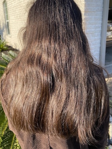
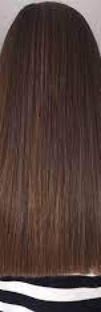
Figure 1. Two representatives in the Identity Morphism

As the name suggests, the braid category is an organisational scheme for braid patterns - for example in hair. The object class is the skeletal one for this problem - the set ${\mathbb{N}}_{0}$ of possible numbers of hairs on a head. The key notion is the appropriate notion of equivalence on concrete braids, so that a morphism is an equivalence class. The picture in Figure 1 illustrates this by showing concrete braids in the same class. (In case the reader imagines that this construction is somehow frivolous, we note that organisational schemes essentially identical to this are vital in making sense of the observable world — see for example [LM77].)

The category composition comes from thinking of transitions from one braid class to another as themselves being braid classes. This is indicated in our schema by the pictures in Figures 2,3, along with the monoidal composition in Figure 4. For corresponding formalism see for example Birman [Bir75] and Mac Lane [Lan78]. Note the category is ‘diagonal’ (endomorphisms only).

Figure 2. A composition of morphisms

 

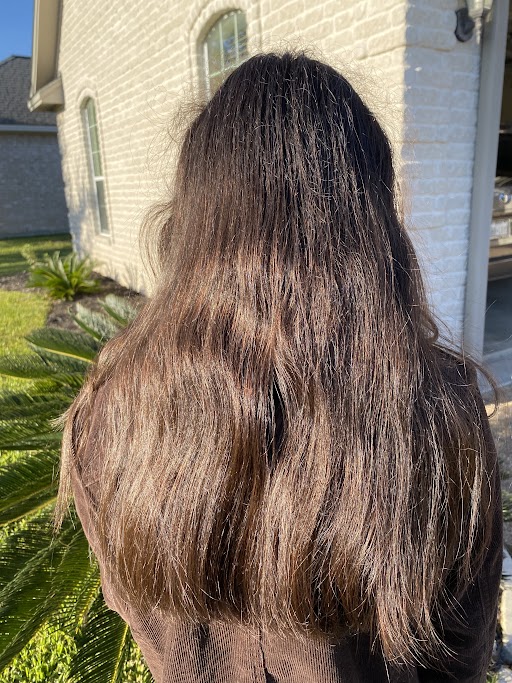
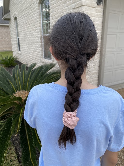
Figure 3. Before and after a sequence of compositions

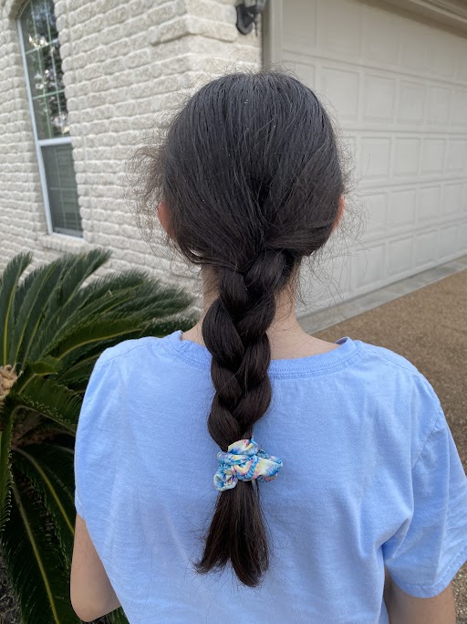
$$\;\;\otimes\;\;$$   =   

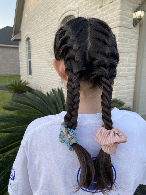
Figure 4. The monoidal product on morphisms

The braid category ${\mathsf{B}}$ is monoidally generated by the elementary braids $\sigma$ and $\sigma^{-1}$ $\in{\mathsf{B}}(2,2)$. Thus a monoidal functor

$$F:{\mathsf{B}}\rightarrow{\mathsf{Match}}^{N}$$

or indeed from ${\mathsf{B}}$ to any target, is determined by the image $F(\sigma)$.

Our monoidal category ${\mathsf{B}}$ has its geometrical definition above. But in order to verify functors it is useful to recall a finite presentation.

A natural monoidal category is one whose object monoid is $({\mathbb{N}},+)$ (confer [Lan65]).

Definition 2.1.

The natural strict monoidal category ${\mathsf{B}}^{\prime}$ is that presented by generators $\varsigma$ and $\varsigma_{-}\in{\mathsf{B}}^{\prime}(2,2)$; and relations as follows. We write $1_{n}$ for the identity morphism in ${\mathsf{B}}^{\prime}(n,n)$; $\varsigma_{1}=\varsigma\otimes 1_{1}$; $\varsigma_{2}=1_{1}\otimes\varsigma$ in ${\mathsf{B}}^{\prime}(3,3)$. Relations are:

$$\varsigma\;\varsigma_{-}\;=\;1_{2}\;=\;{\varsigma_{-}}\;\varsigma$$ (1)

$$\;\;\;\varsigma_{1}\varsigma_{2}\varsigma_{1}=\varsigma_{2}\varsigma_{1}\varsigma_{2}\hskip 21.68121pt\mbox{ that is }\hskip 24.57153pt(\varsigma\otimes 1_{1})(1_{1}\otimes\varsigma)(\varsigma\otimes 1_{1})=(1_{1}\otimes\varsigma)(\varsigma\otimes 1_{1})(1_{1}\otimes\varsigma).$$ (2)

Via Artin’s local presentation [Art25] we have the following.

Proposition 2.2.

A presentation for ${\mathsf{B}}$ is given by ${\mathsf{B}}\cong{\mathsf{B}}^{\prime}$ where $\sigma\mapsto\varsigma$. ∎

3. Target categories and representation theory generalities

‘Charge-conserving’ representation theory as developed here has several novel features compared to, for example, classical Artinian representation theory. Artinian representation theory — representation theory of finite-dimensional algebras over an algebraically closed field $k$ — can be understood as inheriting features from the appropriate target category ${\mathsf{Vect}}_{k}$ (cf. for example [Par70] and also [BB17]).

In as much as representation theory of some algebraic structure $A$ say is the study of the appropriate functor category between $A$ and the target $\mathsf{V}$ say, so representation theory tends to inherit certain properties from $\mathsf{V}$. For example if $A$ is a finite group, regarded as a category with one object, then the functor category $\mathfrak{Func}(A,{\mathsf{Vect}}_{k})$ inherits abelianness from ${\mathsf{Vect}}_{k}$, from which we derive the Jordan–Holder and Krull-Schmidt properties. These properties tell us that classification of representations should proceed through classification of isomorphism classes of irreducible representations and the decomposition series of indecomposable projective representations. In the Artinian setting the theorems appear directly and the categorical perspective is just nice abstract nonsense. In more ‘rigid’ settings such as ours, it can be proactively helpful.

Before proceeding the reader will therefore need to consider the definition and properties of ${\mathsf{Match}}^{N}$ that we discuss in Section 3.1 et seq. We will return to discuss the corresponding analogues of Jordan–Holder, irreducibility, isomorphism etc in Section 0.C.3.

3.1. On the target category ${\mathsf{Match}}^{N}$

 

(3.1) If $A$ and $B$ are matrices, let $A\otimes B$ denote the Ab-convention Kronecker product (see e.g. [Mur38, Ch.3]); and $A\overline{\otimes}B=B\otimes A$ the aB-convention Kronecker product.

Here ${\mathsf{Mat}}$ is the monoidal category of matrices over a given commutative ring (and ${\mathsf{Mat}}_{k}$ the case over commutative ring $k$), with object monoid $(\mathbb{N},\times)$ and tensor product on morphisms given by the aB Kronecker product. We write $\overline{{\mathsf{Mat}}}$ for the monoidal category with $\overline{\otimes}$.

(3.2) For $N\in\mathbb{N}$ the monoidal subcategory ${\mathsf{Mat}}^{N}$ of ${\mathsf{Mat}}$ is that generated by a single object $N$. Then the object monoid $(N^{\mathbb{N}_{0}},\times)$ is isomorphic to $(\mathbb{N}_{0},+)$ in the natural way, so that ${\mathsf{Mat}}^{N}(a,b)={\mathsf{Mat}}(N^{a},N^{b})$.

A monoidal category is ‘natural’ if the object monoid is freely generated by a single object, denoted 1 (thus ${\mathsf{Mat}}^{N}$ is natural). Note that if a monoidal category $C$ is natural then every monoidal functor $F:C\rightarrow{\mathsf{Mat}}$ factors through ${\mathsf{Mat}}^{N}$ for some $N=F(1)$.

(3.3) Let $\mu$ be an invertible $N\times N$ matrix. We write $\overline{\mu}$ for the inverse here, to neaten superscripts. Note that the ‘local base change’ given (on object 1 in the new $(\mathbb{N}_{0},+)$ labelling) by $\mu$ induces a monoidal functor

$${\mathsf{C}}^{\mu}:{\mathsf{Mat}}^{N}\rightarrow{\mathsf{Mat}}^{N}$$

by taking $T\in{\mathsf{Mat}}^{N}(a,b)$ to $(\mu^{\otimes a})\;T\;(\overline{\mu}^{\otimes b})$. Thus ${\mathsf{C}}^{\nu}\circ{\mathsf{C}}^{\mu}={\mathsf{C}}^{\nu\mu}$. That is, the object monoid of functor category $\mathfrak{Func}({\mathsf{Mat}}^{N},{\mathsf{Mat}}^{N})$ contains a realisation of $GL_{N}=GL_{N}(k)$ (see e.g. [Mar08]).

Thus for any monoidal functor $F:{\mathsf{B}}\rightarrow{\mathsf{Mat}}^{N}$, say, and any $\mu$ there is another monoidal functor $F^{\mu}:{\mathsf{B}}\rightarrow{\mathsf{Mat}}^{N}$ given by applying the ‘diagonal’ action: $F^{\mu}={\mathsf{C}}^{\mu}\circ F$.

(3.4) For $N\in{\mathbb{N}}_{0}$ let $\underline{N}=\{1,2,...,N\}$. Let ${\mathsf{Set}}$ be the category of sets; and ${\mathsf{Set}}^{i}(S,T)\subset{\mathsf{Set}}(S,T)$ the subset of isomorphisms. Let $\Sigma_{N}$ denote the symmetric group. Thus $\Sigma_{N}={\mathsf{Set}}^{i}(\underline{N},\underline{N})$.

For $S$ a set, let $S^{n}$ denote the set of sequences of length $n$ of elements from $S$. Equivalently, $S^{n}={\mathsf{Set}}(\underline{n},S)$. If $S$ is a set of symbols then $S^{n}$ can be represented as the set of words $s_{1}s_{2}\cdots s_{n}$ of length $n$ in $S$. Let $S^{\ast}$ denote the set of all words and $S^{\star}$ all non-empty words:

$$S^{\star}=\bigsqcup_{n\in{\mathbb{N}}}S^{n}\hskip 28.45274pt\mbox{ and }\hskip 28.45274ptS^{\ast}=\bigsqcup_{n\in{\mathbb{N}}_{0}}S^{n}$$

(3.5) We may label the row/column index for object $N$ in ${\mathsf{Mat}}$ (object 1 in ${\mathsf{Mat}}^{N}$) by $\mathfrak{e}_{\underline{N}}=\{\mathfrak{e}_{1},\mathfrak{e}_{2},...,\mathfrak{e}_{N}\}$ (or as ‘charges’ $\{+,-\}$ if $N=2$). Note that the ‘standard ordering’ is arbitrary. Thus for $\omega\in\Sigma_{N}$ there is a monoidal functor $f^{\omega}:{\mathsf{Mat}}^{N}\rightarrow{\mathsf{Mat}}^{N}$ given by $f^{\omega}={\mathsf{C}}^{\rho(\omega)}$, where $\rho(\omega)$ is the perm matrix of $\omega$. This is the obvious copy of $\Sigma_{N}$ in our $GL_{N}$.

Remark: Choosing index sets allows us to use the language of linear algebra. For a matrix $\alpha\in{\mathsf{Mat}}(N,M)$ we may write $\alpha\mathfrak{e}_{i}=\sum_{j\in\underline{M}}\alpha_{ij}\mathfrak{e}_{j}$ to give an individual row. (We call this the ‘(right) action’ of $\alpha$, as if it were a linear operator. Think of $\mathfrak{e}_{i}\in{\mathsf{Mat}}(M,1)$ (an elementary column vector).)

In ${\mathsf{Mat}}^{2}$, say, the object $2\otimes 2$ has ‘tensor’ index set $\{\mathfrak{e}_{1}\otimes\mathfrak{e}_{1},\mathfrak{e}_{2}\otimes\mathfrak{e}_{1},\mathfrak{e}_{1}\otimes\mathfrak{e}_{2},\mathfrak{e}_{2}\otimes\mathfrak{e}_{2}\}$ (which we may abbreviate to $\{|11\rangle,|21\rangle,|12\rangle,|22\rangle\}$, or even just $\{11,21,12,22\}$) and so on. Thus the tensor index set for rows of $\alpha\in{\mathsf{Mat}}^{N}(M,M)$, say, is given by the set $\underline{N}^{M}$ of words in $\{1,2,...,N\}$ of length $M$. Note that $\Sigma_{M}$ acts on this set by place permutation.

(3.6) Fix $N$. We say a matrix $\alpha$ in ${\mathsf{Mat}}^{N}(M,M)$ is charge-conserving when $\alpha_{ij}\neq 0$ implies $j=\omega(i)$ for some $\omega\in\Sigma_{M}$. That is, $\alpha$ is a (reordered) block matrix with blocks given by ‘charge’ (orbits of the $\Sigma_{M}$ action on $\underline{N}^{M}$, which are, note, indexed by compositions of $M$).

Lemma 3.7.

Fix $N$ and $k$ (by default $k=\mathbb{C}$).
(I) The charge-conserving matrices form a (diagonal) monoidal subcategory ${\mathsf{Match}}^{N}$ of ${\mathsf{Mat}}^{N}$.
(II) Let $w\in\Sigma_{N}$. The functor $f^{w}$ restricts to a monoidal functor on ${\mathsf{Match}}^{N}$:

$$f^{w}:{\mathsf{Match}}^{N}\rightarrow{\mathsf{Match}}^{N}.$$ (3)

(III) For each $M\leq N$ and each injective function $\psi:\underline{M}\rightarrow\underline{N}$ there is a monoidal functor $f^{\psi}:{\mathsf{Match}}^{N}\rightarrow{\mathsf{Match}}^{M}$ given on morphisms by $f^{\psi}({\mathbf{a}})_{vw}={\mathbf{a}}_{\psi v,\psi w}$ (here ${\mathbf{a}}\in{\mathsf{Match}}^{N}(m,m)$ say).

Proof.

(I) The closure of composition follows in the manner of closure for block diagonal matrices of given block shape, so it remains to show the monoidal property. Consider ${\mathbf{a}}\in{\mathsf{Mat}}^{N}(m,m)$ and ${\mathbf{b}}\in{\mathsf{Mat}}^{N}(m^{\prime},m^{\prime})$. Note that the row index set for ${\mathbf{a}}\otimes{\mathbf{b}}$ is the concatenation $\underline{N}^{m+m^{\prime}}$ (as noted, it is a convention choice for the overall order). Thus if $i$ is a row index for ${\mathbf{a}}$ (an $m$-tuple) and $I$ is a row index for ${\mathbf{b}}$) (an $m^{\prime}$-tuple) then $iI$ is a row index for ${\mathbf{a}}\otimes{\mathbf{b}}$. We have

$$({\mathbf{a}}\otimes{\mathbf{b}})_{iI,jJ}={\mathbf{a}}_{i,j}{\mathbf{b}}_{I,J}$$

Now note that if $j=\omega(i)$ and $J=\omega^{\prime}(I)$ for some perms $\omega\in\Sigma_{m}$ and $\omega^{\prime}\in\Sigma_{m^{\prime}}$ then $jJ=\omega\otimes\omega^{\prime}(iI).$
(II,III) Clear from the construction. ∎

(3.8) Note that if $\mu\in GL_{N}$ is diagonal (in the diagonal maximal torus) then ${\mathsf{C}}^{\mu}$ also restricts to a monoidal functor on ${\mathsf{Match}}^{N}$, but it is trivial. Note that the functors in (II) do not exhaust the set of isomorphisms in the object set of $\mathfrak{Func}({\mathsf{Match}}^{N},{\mathsf{Match}}^{N})$ in general. We can classify such functors as ‘local’ (restrictions of ${\mathsf{C}}^{\mu}$); ‘decomposable’ (asigning a possibly distinct invertible to each tensor factor — see below); and ‘entangled’ (everything else).
On the other hand note that (III) does not extend even to a functor on ${\mathsf{Mat}}^{N}$ in general.
Note that ${\mathsf{Match}}^{N}$ also inherits linearity from ${\mathsf{Mat}}$. Here we will use this only for convenience.

(3.9) Let ${\mathbf{C}}$ be an natural monoidal category generated by $\varSigma\subset{\mathbf{C}}(2,2)$. A level-$N$ monoidal functor ${\mathsf{f}}:{\mathbf{C}}\rightarrow{\mathsf{Mat}}$ is one taking object 1 (in ${\mathbf{C}}$) to $N$ (in ${\mathsf{Mat}}$). The functor is charge-conserving (the image lies in ${\mathsf{Match}}^{N}$) if every generator $\varsigma\in\varSigma$ acts so that $\varsigma|\underline{ij}\rangle$ lies in the span of $|\underline{ij}\rangle,|\underline{ji}\rangle$. In other words we have the following for $\varsigma\in\varSigma$ (e.g. the positive braid in ${\mathsf{B}}(2,2)$):

$$\varsigma|\underline{11}\rangle=a_{11}|\underline{11}\rangle,\hskip 9.46712pt\varsigma|\underline{12}\rangle=a_{12}|\underline{12}\rangle+b_{12}|\underline{21}\rangle,\hskip 9.39545pt\varsigma|\underline{21}\rangle=c_{12}|\underline{12}\rangle+d_{12}|\underline{21}\rangle,\hskip 9.46712pt\varsigma|\underline{22}\rangle=a_{22}|\underline{22}\rangle$$ (4)

for some $a_{11},a_{12},b_{12},c_{12},d_{12},a_{22}\in k$; and similarly replacing 12 with each $ij$, with $i<j$.

(3.10) Calculus for operators in the monoidal category, such as $\varsigma_{1}=\varsigma\otimes 1$, is exemplified by:

$$\varsigma_{1}|\underline{112}\rangle=(\varsigma\otimes 1)|\underline{112}\rangle=a_{11}|\underline{112}\rangle,\hskip 73.354pt\varsigma_{2}|\underline{112}\rangle=(1\otimes\varsigma)|\underline{112}\rangle=a_{12}|\underline{112}\rangle+b_{12}|\underline{121}\rangle$$

$$(\varsigma\otimes 1)|\underline{121}\rangle=a_{12}|\underline{121}\rangle+b_{12}|\underline{211}\rangle\hskip 109.85071pt(1\otimes\varsigma)|\underline{121}\rangle=c_{12}|\underline{112}\rangle+d_{12}|\underline{121}\rangle$$

$$(\varsigma\otimes 1)|\underline{211}\rangle=c_{12}|\underline{121}\rangle+d_{12}|\underline{211}\rangle\hskip 109.85071pt(1\otimes\varsigma)|\underline{123}\rangle=a_{23}|\underline{123}\rangle+b_{23}|\underline{132}\rangle$$

$$\varsigma_{1}\varsigma_{2}\varsigma_{1}|\underline{123}\rangle=a_{12}(a_{23}(a_{12}|\underline{123}\rangle+b_{12}|\underline{213}\rangle)+b_{23}(a_{13}|\underline{132}\rangle+b_{13}|\underline{312}\rangle))$$

$$\hskip 72.26999pt+b_{12}(a_{13}(d_{12}|\underline{213}\rangle+c_{12}|\underline{123}\rangle)+b_{13}(a_{23}|\underline{231}\rangle+b_{23}|\underline{321}\rangle))$$ (5)

$$\varsigma_{2}\varsigma_{1}\varsigma_{2}|\underline{123}\rangle=a_{23}(a_{12}(a_{23}|\underline{123}\rangle+b_{23}|\underline{132}\rangle)+b_{12}(a_{13}|\underline{213}\rangle+b_{13}|\underline{231}\rangle))$$

$$\hskip 72.26999pt+b_{23}(a_{13}(d_{23}|\underline{132}\rangle+c_{23}|\underline{123}\rangle)+b_{13}(a_{12}|\underline{312}\rangle+b_{12}|\underline{321}\rangle))$$ (6)

(3.11) For later reference, the conditions for the actions in (5), (6) to be equal are thus

$$a_{12}^{2}a_{23}+a_{13}b_{12}c_{12}\stackrel{{\scriptstyle 123}}{{=}}a_{12}a_{23}^{2}+a_{13}b_{23}c_{23},$$ (7)

$$(a_{12}a_{13}-a_{23}a_{12}-a_{13}d_{23})b_{23}\stackrel{{\scriptstyle 132}}{{=}}0,\hskip 72.26999pt(a_{12}a_{23}+a_{13}d_{12}-a_{23}a_{13})b_{12}\stackrel{{\scriptstyle 213}}{{=}}0$$ (8)

Actions on any $|\underline{ijk}\rangle$ can be computed similarly, or by applying $\Sigma_{N}$. For $|\underline{112}\rangle$ and its orbit:

$$(\varsigma\otimes 1)(1\otimes\varsigma)|\underline{112}\rangle=(\varsigma\otimes 1)(a_{12}|\underline{112}\rangle+b_{12}|\underline{121}\rangle)=(a_{11}a_{12}|\underline{112}\rangle+b_{12}(a_{12}|\underline{121}\rangle+b_{12}|\underline{211}\rangle))$$

$$\varsigma_{2}\varsigma_{1}\varsigma_{2}|\underline{112}\rangle=(a_{11}a_{12}(a_{12}|\underline{112}\rangle+b_{12}|\underline{121}\rangle)+b_{12}(a_{12}(d_{12}|\underline{121}\rangle+c_{12}|\underline{112}\rangle)+a_{11}b_{12}|\underline{211}\rangle))$$

$$\varsigma_{2}\varsigma_{1}\varsigma_{2}|\underline{121}\rangle=(a_{11}c_{12}(a_{12}|\underline{112}\rangle+b_{12}|\underline{121}\rangle)+d_{12}(a_{12}(d_{12}|\underline{121}\rangle+c_{12}|\underline{112}\rangle)+a_{11}b_{12}|\underline{211}\rangle))$$

$$\varsigma_{1}\varsigma_{2}\varsigma_{1}|\underline{121}\rangle=a_{12}(a_{11}c_{12}|\underline{112}\rangle+d_{12}(a_{12}|\underline{121}\rangle+b_{12}|\underline{211}\rangle)+a_{11}b_{12}(d_{12}|\underline{211}\rangle+c_{12}|\underline{121}\rangle))$$

Thus for example a condition ${\mathsf{f}}(\varsigma_{1}\varsigma_{2}\varsigma_{1})={\mathsf{f}}(\varsigma_{2}\varsigma_{1}\varsigma_{2})$ would imply (with $\underline{12}\leadsto\underline{ij}$ for all $i<j$ etc.)

$$(a_{11}^{2}a_{12}-a_{11}a_{12}^{2}-b_{12}c_{12}{a_{12}})|\underline{112}\rangle=0,\hskip 73.7157ptd_{12}a_{12}b_{12}|\underline{121}\rangle=0$$ (9)

$$(d_{12}a_{12}c_{12})|\underline{112}\rangle=0,\hskip 22.40352pt(d_{12}^{2}a_{12}-a_{12}^{2}d_{12})|\underline{121}\rangle=0,\hskip 20.95781pta_{12}d_{12}b_{12}|\underline{211}\rangle=0$$ (10)

Noting Proposition 2.2, these cubics are the residue in this setting of the intractable problem described in the Introduction. While still daunting, they do now yield better to analysis.

Theorem 3.12.

Let ${\mathsf{F}}:{\mathsf{B}}\rightarrow{\mathsf{Match}}^{N}$ be a level-$N$ charge-conserving monoidal functor, thus determined by $F(\sigma)$. The condition $(\sigma\otimes 1)(1\otimes\sigma)(\sigma\otimes 1)=(1\otimes\sigma)(\sigma\otimes 1)(1\otimes\sigma)$ (from 2.2) is equivalent to the following constraints on entries in the $abcd$ form (equation (4)) of $F(\sigma)$:

$$a_{12}(a_{11}^{2}-a_{12}a_{11}-b_{12}c_{12})=0,\hskip 28.45274pta_{12}(a_{22}^{2}-a_{12}a_{22}-b_{12}c_{12})=0,$$ (11)

$$\hskip 28.45274pta_{12}c_{12}d_{12}=0=a_{12}b_{12}d_{12},\hskip 28.45274pta_{12}d_{12}(a_{12}-d_{12})=0,$$ (12)

$$c_{12}(d_{13}d_{23}-d_{12}d_{23}-a_{12}d_{13})=0,\hskip 28.45274ptc_{12}(-a_{13}a_{23}+a_{12}a_{23}+d_{12}a_{13})=0$$ (13)

$$-a_{13}d_{23}^{2}+a_{13}^{2}d_{23}-a_{12}b_{23}c_{23}+a_{12}b_{13}c_{13}=0$$ (14)

together with the images of these constraints which are their orbits under the action of $\Sigma_{N}$ by $\omega a_{ij}=a_{\omega(i)\omega(j)}$ and so on (where $a_{ji}=d_{ij}$ and $b_{ji}=c_{ij}$ is understood).

Proof. Observe that the YBE can be verified in ${\mathsf{Mat}}^{N}(3,3)$ (since it can be formulated with three tensor factors; and the higher versions simply contain copies of the same entries, by the tensor construction). This yields equations across three indices, computed as in (7)-(10). ∎

The following is an immediate consequence, but is a key fact so we record it as:

Lemma 3.13.

A level-$N$ charge-conserving operator $F(\sigma)$ defines a monoidal functor $F:{\mathsf{B}}\rightarrow{\mathsf{Match}}^{N}$ if, and only if all of the ${N\choose 3}$ restrictions of $F$ to ${\mathsf{Match}}^{3}$ satisfy equations (11)-(14) together with the images of these constraints which are their orbits under the action of $\Sigma_{3}$. ∎

(3.14) Lemma. (X Lemma) Let ${\mathsf{F}}:{\mathsf{B}}\rightarrow{\mathsf{Match}}^{N}$ be a braid representation, hence given by ${\mathsf{F}}(\sigma)$. (I) Let $X$ be a diagonal invertible matrix in ${\mathsf{Match}}^{N}(2,2)$. Then ${\mathsf{F}}^{\prime}(\sigma)=X{\mathsf{F}}(\sigma)X^{-1}$ also gives a representation.

(II) The relation: ${\mathsf{F}}\stackrel{{\scriptstyle-}}{{\sim}}{\mathsf{F}}^{\prime}$ if ${\mathsf{F}}^{\prime}(\sigma)=X{\mathsf{F}}(\sigma)X^{-1}$ for some $X$, is an equivalence.
The relation $\stackrel{{\scriptstyle-}}{{\sim}}$ is here called X-equivalence, and written $\stackrel{{\scriptstyle X}}{{=}}$.

Proof. Noting presentation 2.2, this follows from how $b_{ij},c_{ij}$ appear in (7-10). See also (0.B). ∎

The analogue of 3.13 in classical representation theory is stronger, and is elementary and subject independent. Here in the monoidal setting we see that it is not elementary or general.

(3.15) We have a monoidal functor between monoidal categories $\overrightarrow{R}:{\mathsf{Mat}}^{N}\rightarrow\overline{{\mathsf{Mat}}}^{N}$ given by the identity on objects and on morphisms by $\overrightarrow{R}(A)_{v,w}=A_{\overline{v},\overline{w}}$ where $\overline{w}$ is the reverse word.

(3.16) The ‘lateral flip’ inner automorphism on an individual braid group:

$$\overleftrightarrow{{\mathsf{F}}}:B_{n}\rightarrow B_{n}$$ (15)

(see e.g. [Mar91, §5.7.2] or [Hie92]) corresponds, on the braid generators, to $\sigma_{i}\mapsto\sigma_{n-i}$. Note that this extends to an automorphism of ${\mathsf{B}}$, except that the monoidal product convention is reversed, so there we denote it $\overrightarrow{{\mathsf{F}}}:{\mathsf{B}}\rightarrow\overline{{\mathsf{B}}}$. Similarly we have $\overrightarrow{{\mathsf{F}}}:\overline{{\mathsf{B}}}\rightarrow{\mathsf{B}}$. Combining with $\overrightarrow{R}$ we get an involutive action on the functor category $\mathfrak{Func}({\mathsf{B}},{\mathsf{Mat}})$, with generator that we will denote ${\mathtt{P}}$.   Note that this fixes the target subcategory ${\mathsf{Match}}^{N}$.

(3.17) In ordinary representation theory organisation is provided by intertwiners/module morphisms, which are the morphisms in the representation category. In our case this view lifts so that intertwiners between representation-functors are natural transformations. The various key principles of representation theory have lifts to our setting, but these lifts have novel features, as in Lemma 3.7. And then there are features that depend on specific properties of the ‘subject-algebra’ (in our case ${\mathsf{B}}$) such as (3.13), and the following.

The $\mathbb{Z}_{2}$ action from 3.13 fixes the target ${\mathsf{Match}}^{N}$. It and the $\Sigma_{N}$ action induced from 3.7(II) commute, giving an action of $\mathbb{Z}_{2}\times\Sigma_{N}$ on the category of monoidal functors $F:{\mathsf{B}}\rightarrow{\mathsf{Match}}^{N}$.

3.2. Geometrical setup for functors to Match categories

 

The focus of this paper is to classify charge-conserving solutions to the YBE, i.e., monoidal functors $F:{\mathsf{B}}\rightarrow{\mathsf{Match}}^{N}$; and provide the algorithm for producing them.

The braid category is monoidally generated by the elementary braids $\sigma,\sigma^{-1}\in{\mathsf{B}}(2,2)$. Thus a monoidal functor $F:{\mathsf{B}}\rightarrow{\mathsf{Match}}^{N}$ is determined by the image $F(\sigma)\in{\mathsf{Match}}^{N}(2,2)$.

(3.18) Recall that the rows (and columns) of a matrix $M\in{\mathsf{Mat}}^{N}(2,2)$ may be indexed by ordered pairs $(i,j)$ with $i,j\in\underline{N}=\{1,2,...,N\}$. Thus matrix entries are $M_{ij,kl}$. A matrix $M\in{\mathsf{Match}}^{N}(2,2)\subset{\mathsf{Mat}}^{N}(2,2)$ is sparse. The non-zero blocks are $1\times 1$ and $2\times 2$, naturally in correspondence with the vertices $i$ and edges $ij$ respectively of the complete graph $K_{N}$.

                  

Figure 5. (a) The graph $K_{6}$; and (b) conventions for a Higgs configuration on $K_{4}$.

(3.19) For $N\in{\mathbb{N}}$, $K_{N}$ denotes the directed graph with vertex set $\underline{N}=\{1,2,...,N\}$ and an edge $(i,j)$ whenever $i<j$. If $S$ is an ordered set then we write $K_{S}$ for the corresponding complete graph on vertex set $S$.     For example, with $N=6$: see Fig.5(a).

(3.20) A configuration $\boldsymbol{\alpha}$ on $K_{N}$ is an assignment of a variable to each vertex and a $2\times 2$ matrix of variables to each directed edge. By (3.2) this encodes an element of ${\mathsf{Match}}^{N}(2,2)$. See Fig.5(b), where we name matrix entries as in (4), with $a_{i}=a_{ii}$.

We should think of these assignments in this geometrical form. But sometimes it is convenient to give them in-line. Then the order we shall take is with vertex assignments first in the natural order, and then edge assignments in the order 12,13,23,14,24,34 and so on. That is, for $M\in{\mathsf{Match}}^{N}(2,2)$ we may write it, first generally, and then using (4) with $a_{i}=a_{ii}$:

$${\underline{\alpha}}(M)=(M_{11,11},M_{22,22},\ldots,M_{NN,NN},\left(\begin{array}[]{cc}M_{12,12}&M_{12,21}\\ M_{21,12}&M_{21,21}\end{array}\right),\left(\begin{array}[]{cc}M_{13,13}&M_{13,31}\\ M_{31,13}&M_{31,31}\end{array}\right),\ldots)$$ (16)

$$=(a_{1},a_{2},\ldots,a_{N},\left(\begin{array}[]{cc}\!a_{12}&b_{12}\!\\ \!c_{12}&d_{12}\!\end{array}\right)\!,\left(\begin{array}[]{cc}\!a_{13}&b_{13}\\ \!c_{13}&d_{13}\end{array}\right),\ldots)\hskip 115.63243pt$$

$$\hskip 40.61548pt=(a_{1},a_{2},\ldots,a_{N},A(1,2),A(1,3),\ldots,A(N\!-\!1,N)),\hskip 14.45377pt\mbox{ where }A(i,j):=\left(\begin{array}[]{cc}\!\!\!a_{ij}&b_{ij}\!\!\\ \!\!\!c_{ij}&d_{ij}\!\!\end{array}\right)$$

(1)                 (2)                 (3a)                    (3b)                    (4a)                (4b)

Figure 6. Schematic for possible edge submatrices up to X-equivalence.

Proposition 3.21.

For $N=2$ the following gives a complete classification of charge conserving functors ${\mathsf{F}}$ from ${\mathsf{B}}$ up to X-equivalence. We use the coefficient names given by ${\mathsf{F}}(\sigma)=\left(\begin{array}[]{cccc}\!\!a_{1}\!\\ &a_{12}&b_{12}\\ &c_{12}&d_{12}\\ &&&\!a_{2}\!\end{array}\right)$. That is, ${\underline{\alpha}}({\mathsf{F}}(\sigma))=(a_{1},a_{2},{A}(1,2))$. We have:

1. The $0$ case: $a_{1}=a_{12}=d_{12}=a_{2}$, and $b_{12}=c_{12}=0$, i.e., ${\mathsf{F}}(\sigma)=\alpha\cdot Id$, with $\alpha\neq 0$.

2. The $/$ case: $a_{12}=d_{12}=0$, and $a_{1}=\alpha$, $a_{2}=\beta$ and $b_{12}=c_{12}=\mu$, say, with $\alpha,\beta,\mu\neq 0$.

3. The $+$ cases: $d_{12}=0$, $a_{12}=\alpha+\beta$, $b_{12}=1$, $c_{12}=-\alpha\beta$ where $\alpha+\beta\neq 0$ and either

   1. ${\mathsf{a}}$ case: $a_{1}=\alpha\neq a_{2}=\beta$ or

   2. ${\mathsf{f}}$ case: $a_{1}=a_{2}=\alpha$

4. The $-$ cases: $a_{12}=0$, $d_{12}=\alpha+\beta$, $b_{12}=1$, $c_{12}=-\alpha\beta$ where $\alpha+\beta\neq 0$ and either

   1. $\underline{{\mathsf{a}}}$ case: $a_{1}=\alpha\neq a_{2}=\beta$ or

   2. $\underline{{\mathsf{f}}}$ case: $a_{1}=a_{2}=\alpha$.

NB, the $/$ and ${\mathsf{f}},{\mathsf{a}}$ varieties ‘touch’, but the given partition is good for treating higher ranks, as we shall see. Possible edge submatrices are as shown in Figure 6. (The labels ${\mathsf{f}}$ and ${\mathsf{a}}$ are taken from ferromagnetic and anti-ferromagnetic, indicating if vertex labels are the same or not.)

(3.22) Proof. Equations (11-(12) (and their images under the action of $\Sigma_{2}$) are relevant for $N=2$. Under the transposition $(1\/2)\in\Sigma_{2}$ we obtain similar equations but with $a_{12}$ and $d_{12}$ interchanged. Observe that $a_{1},a_{2}$ and $a_{12}d_{12}-b_{12}c_{12}$ are non-zero by invertibility. We take it case by case to find necessary and sufficient conditions for these constraints.

If $b_{12}c_{12}=0$ then $a_{12}d_{12}\neq 0$, so the equations imply $a_{12}=d_{12}=a_{1}=a_{2}$, which is case $0$. It is routine to check that this indeed gives a solution for any nonzero value.

If $b_{12}c_{12}\neq 0$ then there are 3 cases to consider: $a_{12}=d_{12}=0$ or exactly one of $a_{12}$ or $d_{12}$ is non-zero. In the first case all equations are satisfied, so that $a_{1},a_{2},b_{12},c_{12}$ may be chosen arbitrarily. The X transformation then allows $b_{12}=c_{12}$, so this gives the $/$ case.

Next suppose that $b_{12}c_{12}a_{12}\neq 0$, and $d_{12}=0$. This implies that $b_{12}c_{12}=a_{2}(a_{12}-a_{2})=a_{1}(a_{12}-a_{1})$. Now the characteristic polynomial of the $2\times 2$ matrix (call it $A(1,2)$) is $x^{2}-a_{12}x-b_{12}c_{12}$ so that $a_{1}$ and $a_{2}$ are eigenvalues of $A(1,2)$. Let $\alpha,\beta$ be these eigenvalues. Since $Tr(A(1,2))=a_{12}$ we have that $a_{12}=\alpha+\beta$, and similarly $Det(A(1,2))=-b_{12}c_{12}=\alpha\beta$. Using the X transformation we may assume that $b_{12}=-\alpha\beta$ and $c_{12}=1$ or vice versa. Notice that the only restriction on $\alpha,\beta$ is that $\alpha+\beta\neq 0$. Now there are two cases, up to the obvious labeling ambiguity of $\alpha$ and $\beta$: either $a_{1}=a_{2}=\alpha$ (case ${\mathsf{f}}$) or $a_{1}=\alpha$ and $a_{2}=\beta$ (case ${\mathsf{a}}$).

The case $a_{12}=0$ is completely analogous: we find that $d_{12}=\alpha+\beta$, and $b_{12}=-\alpha\beta$, $c_{12}=1$ (or vice versa) and $a_{1}=a_{2}=\alpha$ (case $\underline{\mathsf{f}}$) or $a_{1}=\alpha$ and $a_{2}=\beta$ (case $\underline{\mathsf{a}}$).

In any of the last 4 cases it is possible that $\alpha=\beta$, whereupon the ${\mathsf{f}}$ case prevails. ∎

4. Constructions for the main Theorem

We write $\Lambda_{N}$ for the set of integer partitions of $N$. We may write $\lambda\vdash N$ for $\lambda\in\Lambda_{N}$.

4.1. How to read the classification Theorem 4.12:

 

An example of a classification theorem is of course Young’s classification of irreducible representations of the symmetric group over $\mathbb{C}$. Here one says that irreducible representations of $\Sigma_{n}$ may be classified up to isomorphism by the set $\Lambda_{n}$. Each of the three aspects of this formulation flags challenges that we must address in our problem.

Firstly, analogously to the integer partitions we will need to introduce some combinatorial structures. (Our Theorem also gives a construction. We will introduce notation for this too.)

Secondly, group/algebra representations form an additive category in a natural way. The category property yields a ‘good’ notion of isomorphism. The additive property simultaneously implies that there are unboundedly many classes of representations, but also that these can be effectively classified by classifying their additive components. There is no canonical lift of these properties to the monoidal category setting (confer for example [MM16, MM14, RW18, KV94]), so our lift sheds new light on this aspect of higher representation theory.

And finally, treated individually symmetric group algebras over algebraically closed fields are Artinian, so the Jordan–Holder property tells us that every representation has a decomposition series with irreducible factors. Indeed in the complex case the decomposition multiplicities characterise a representation up to isomorphism. There is no canonical lift of this property to monoidal categories either (roughly since decomposition series are additive decompositions, while the monoidal structure is multiplicative). This is one of the places where the rigidity of the ${\mathsf{Match}}^{N}$ target categories saves the day — we will be able to classify all representations directly.

Next we construct two sets for each $N\in{\mathbb{N}}$. One is the set ${\mathfrak{S}}_{N}$ to which we may apply an algorithm (given in (4.2)) to construct all varieties of solutions at level-$N$. The other gives a transversal of this set under the $\Sigma_{N}$ action from (3.13) (and frames the effect of the $\mathbb{Z}_{2}$ action), thus addressing the classification up to isomorphism.

4.2. Braid representations from multisets of row-2-coloured Young diagrams

 

Just as multisets of integers - represented as Young diagrams - index $\Sigma_{N}$ representations, we will see that for braid representations we can use multisets of row-2-coloured composition diagrams. In fact these are a natural combinatorial generalisation of $\Lambda_{N}$. First we explain this combinatoric; then we show how each diagram leads to a class of charge-conserving braid representations; then we prove that this construction exhausts the set of all such braid representations.

(4.1) Given a set $\Omega$ and a map $\psi\in{\mathsf{Set}}(\Omega,{\mathbb{N}})$ define the sets of multisets of total degree $N$:

$$J_{N}(\Omega)=J_{N}(\Omega,\psi)=\{f\in{\mathsf{Set}}(\Omega,{\mathbb{N}}_{0})\;|\;\sum_{w\in\Omega}f(w)\psi(w)=N\}$$

Thus for example if $\Omega={\mathbb{N}}$ and $\psi(n)=n$ then $J_{N}({\mathbb{N}})=\Lambda_{N}$.

(4.2) For $S$ a set, define $\psi:S^{*}\rightarrow{\mathbb{N}}$ by $\psi(w)=length(w)+1$. (Cf. (3.1).) Observe that up to isomorphism $J_{N}(S^{*})$ depends only on the cardinality of $S$. Consider $J_{N}(S^{*})$ for $S=\{1\}$, $\{1,2\},\{1,2,3\}$ and so on.

Of course $\psi:\{1\}^{*}\stackrel{{\scriptstyle\sim}}{{\rightarrow}}{\mathbb{N}}$. So $J_{N}(\{1\}^{*})$ is a realisation of $\Lambda_{N}$. For example $f\in{\mathsf{Set}}(\{1\}^{\star},{\mathbb{N}}_{0})$ given by $f(1)=1$; $f(11)=2$; $f(w)=0$ otherwise, becomes $(3,3,2)\vdash 8$.

In this $J_{N}(S^{*})$ notation, $\{1,2\}^{N}$ encodes the set $\Gamma_{N}$ of compositions of $N$ (via the ${\mathsf{j}}$-function given just below); and $\{1,2\}^{*}$ encodes the set $\Gamma$ of all compositions; so $J_{N}(\{1,2\}^{*})$ encodes the set of multisets of compositions of total degree $N$.

The set we need — of multisets of 2-coloured compositions — is $J_{N}(\{1,2,3\}^{*})$. The construction works as follows. Firstly $\Gamma^{2}_{N}$ denotes the set of 2-coloured compositions of $N$, whose elements are compositions of $N$ together with a two-part partition of the components. We may draw $\lambda\in\Gamma^{2}_{N}$ as a stack of rows of boxes, where the top row is unshaded but other rows can be unshaded or shaded (in the first or second part respectively). For example: $\in\Gamma^{2}_{7}$, and see Fig.10. (This box formulation is useful, but note columns have no significance, cf. ordinary Young diagrams.) Next we show that $\{1,2,3\}^{*}$ encodes the set $\Gamma^{2}$ of all 2-coloured compositions.

(4.3) Given a 2-coloured composition or equivalently a row-2-coloured Young/composition diagram $\lambda\in\Gamma_{N}^{2}$ then diagram ${\mathsf{j}}_{1}(\lambda)\in\Gamma_{N+1}^{2}$ is obtained by adding a box to the last row; ${\mathsf{j}}_{2}(\lambda)\in\Gamma_{N+1}^{2}$ is obtained by adding a box in a new unshaded row; and ${\mathsf{j}}_{3}(\lambda)\in\Gamma_{N+1}^{2}$ is obtained by adding a box in a new shaded row. Starting with the one-box (unshaded) diagram, a word $w\in\{1,2,3\}^{*}$ then defines a row-2-coloured diagram by applying the ${\mathsf{j}}_{i}$ maps in the sequence given by $w$. That is ${\mathsf{j}}:\{1,2,3\}^{n}\rightarrow\Gamma_{n+1}^{2}$ is given by $w_{1}w_{2}...w_{n}\mapsto{\mathsf{j}}_{w_{n}}\circ...\circ{\mathsf{j}}_{w_{2}}\circ{\mathsf{j}}_{w_{1}}(\square)$. Thus ${\mathsf{j}}(121311)$ is given by $\square\stackrel{{\scriptstyle{\mathsf{j}}_{1}}}{{\mapsto}}\includegraphics[width=15.07993pt]{xfig/y2.eps}\stackrel{{\scriptstyle{\mathsf{j}}_{2}}}{{\mapsto}}\includegraphics[width=15.07993pt]{xfig/y21.eps}\stackrel{{\scriptstyle{\mathsf{j}}_{1}}}{{\mapsto}}\includegraphics[width=15.07993pt]{xfig/y22.eps}\stackrel{{\scriptstyle{\mathsf{j}}_{3}}}{{\mapsto}}\includegraphics[width=15.07993pt]{xfig/y221.eps}\stackrel{{\scriptstyle{\mathsf{j}}_{1}}}{{\mapsto}}\includegraphics[width=15.07993pt]{xfig/y222.eps}\stackrel{{\scriptstyle{\mathsf{j}}_{1}}}{{\mapsto}}\includegraphics[width=22.27864pt]{xfig/y223.eps}$ and so on. Note from the construction that ${\mathsf{j}}$ is reversible and hence a bijection in each rank.

(4.4) Note that $f\in J_{N}(\{1,2,3\}^{*})$ assigns a multiplicity $f(w)$ to each word $w$ and hence diagram ${\mathsf{j}}(w)$, such that the total degree is $N$. We will show how each such $f$ corresponds to an equivalence class of varieties of configurations on $K_{N}$, and hence matrices that give the functors ${\mathsf{F}}:{\mathsf{B}}\rightarrow{\mathsf{Match}}^{N}$.

Firstly we arrange 2-coloured composition diagrams in multiplicities as given by $f$, so that we have $N$ boxes altogether. For example with $f$ given by $f(1321)=1$, $f(131)=1$, $f(\emptyset)=2$ and $f(w)=0$ otherwise we obtain an 11-box composite diagram such as:

$${\mathsf{j}}(f)\;=\;\;\raisebox{-15.17719pt}{ \includegraphics[width=83.65117pt]{xfig/tree012ex10bbb1XI0.eps} }$$ (17)

Secondly we assign the $N$ vertices of $K_{N}$ to these $N$ boxes. For example:

$${\mathsf{j}}(f)\;\mapsto\;\;\raisebox{-15.17719pt}{ \includegraphics[width=99.41402pt]{xfig/tree012ex10bbb1XI.eps} }$$ (18)

Write ${\mathfrak{S}}_{N}$ for the set of all assignments up to the order within each row. Thus

$${\mathfrak{S}}_{2}=\{\;\includegraphics[width=22.76228pt]{xfig/tree012ex2aab.eps}\;,\;\;\includegraphics[width=11.66573pt]{xfig/tree012ex2ab1b.eps}\;,\;\;\includegraphics[width=11.66573pt]{xfig/tree012ex2ba1b.eps}\;,\;\;\includegraphics[width=11.66573pt]{xfig/tree012ex2abb.eps}\;,\;\;\includegraphics[width=11.66573pt]{xfig/tree012ex2bab.eps}\;,\;\;\includegraphics[width=29.30629pt]{xfig/tree012ex2acb.eps}\;\}.$$ (19)

We can choose any such assignment for each $f$. But it will be convenient to have a prefered assignment, of vertices in ‘book’ order as in (18). This requires the diagrams in a composite to be written in a specific sequence. We can do this using a declared total order on $\Gamma^{2}$ (or equivalently on $\{1,2,3\}^{*}$) — noting that identical diagrams are indistinguishable.

For a total order on $\{1,2,3\}^{*}$ let us say firstly that longer sequences come before shorter ones: $111<11<1$ and so on; and for equal-length sequences we use dictionary order, that is $111<112<113<121<...<333$. Then we get our example ${\mathsf{j}}(f)$ in (17) above, and hence (18), on the nose. Write ${\mathsf{b}}:{\mathsf{j}}(J_{N}(\{1,2,3\}^{*}))\rightarrow{\mathfrak{S}}_{N}$ for the book order assignment. Define ${\mathfrak{T}}_{N}={\mathsf{b}}({\mathsf{j}}(J_{N}(\{1,2,3\}^{*})))$. For example ${\mathfrak{T}}_{2}=\{\;\includegraphics[width=22.76228pt]{xfig/tree012ex2aab.eps}\;,\;\;\includegraphics[width=11.66573pt]{xfig/tree012ex2ab1b.eps}\;,\;\;\includegraphics[width=11.66573pt]{xfig/tree012ex2abb.eps}\;,\;\;\includegraphics[width=29.30629pt]{xfig/tree012ex2acb.eps}\;\}$.

There is a correspondence between ${\mathfrak{S}}_{2}$ and our classification for $N=2$ in Prop.3.21. The rest of our exposition amounts to showing ${\mathfrak{S}}_{N}$ yields an index scheme for all varieties of representations. Noting Lemma 3.7(III), the $N=2$ solutions also give the possible edge configurations for all $N$.

(4.5) Given a set $S$ we will write ${\mathsf{P}}(S)$ for the set of partitions; and ${\mathsf{P}}_{2}(S)$ for the set of partitions into at most 2 parts. If $N\in{\mathbb{N}}$ then ${\mathsf{P}}(N)={\mathsf{P}}(\underline{N})$.

“Children-first order”: Given a partition $p$ of $\{1,2,...,N\}$ (or any subset thereof), we will order the parts according to their lowest numbered element; and write $p_{i}$ for the $i$th such part.

(4.6) A refinement of set partition $p$ is a further partition of the parts of $p$ (‘nations’, say) into possibly smaller parts (‘counties’, say). We will write $p<q$ (or $q>p$) if $q$ is a refinement of $p$.
We may write $q|p_{i}$ for the restriction of $q$ to the partition of $p_{i}$.

(4.7) Next we need a recipe for constructing a variety of elements of ${\mathsf{Match}}^{N}(2,2)$ that give solutions ${\mathsf{F}}(\sigma)$ from an element of ${\mathfrak{S}}_{N}$. An element of ${\mathfrak{S}}_{N}$ can be viewed in various ways. Firstly it encodes a partition $p$ of the vertices into the individual diagrams — ‘nations’; and a refinement $q$ of that partition into rows — ‘counties’. It also gives a total order $\rho$ on the rows in each nation, from top to bottom; and a partition $s$ of them into two parts, according to shaded or not.

This formulation $(p,q,\rho,s)$ will control the varieties upon which our representations will lie.

(4.8) The following example is in ${\mathfrak{S}}_{12}$ (but not ${\mathfrak{T}}_{12}$):

$$\lambda=\;\;\raisebox{-14.45377pt}{ \includegraphics[width=89.626pt]{xfig/tree012ex12x157x.eps}}$$ (20)

The $(p,q,\rho,s)$ form of $\lambda$ as in (20) has $\;p=\{\{1,3,4,5,7,9\},\{2,6,X\},\{8,X\!\!I,X\!\!I\!\!I\}\}\;$ and $\;q=\{\{1,5,7\},\{3,9\},\{4\},\{6\},\{2,X\},\{X\!\!I\},\{8,X\!\!I\!\!I\}\}$; and the order $\rho$ of the counties in the first nation happens to be the nominal children-first order; and, just focussing on the first nation, $s$ given by lumping the first two counties together.

(4.9) Consider $\lambda\in{\mathfrak{S}}_{N}$ in the form $(p,q,\rho,s)$. Order/number parts of $p$ as in (4.2). Consider the complete graph $K_{p}$ on the ordered set $p$. We associate a variable $\mu_{ij}$ to each edge, i.e. to each pair $p_{i},p_{j}\in p$ with $i<j$; and a variable $\alpha_{i}$ to each vertex $p_{i}$; and a variable $\beta_{i}$ to each vertex $p_{i}\in p$ containing more than one part of $q$. (NB the given names of variables serve to distinguish them, but have no extrinsic significance.)

The type-space $\mathbb{C}^{(p,q)}$ of $(p,q,\rho,s)\in{\mathfrak{S}}_{N}$ is the space whose elements give an evaluation of each variable to an element of $\mathbb{C}^{\times}$, a nonzero complex number, such that $\beta_{i}\neq-\alpha_{i}$. That is the complex space of variables excluding only the variety $\prod_{ij}\mu_{ij}\prod_{i}\alpha_{i}\beta_{i}(\alpha_{i}+\beta_{i})$.
A germ is a pair consisting of an element $(p,q,\rho,s)\in{\mathfrak{S}}_{N}$ and an element from $\mathbb{C}^{(p,q)}$. Write ${\mathfrak{S}}^{\mathbb{C}}_{N}$ for the set of germs. Write ${\mathfrak{T}}^{\mathbb{C}}_{N}$ for the subset of germs derived from $(p,q,\rho,s)\in{\mathfrak{T}}_{N}$.

(4.10) The recipe

$${\mathsf{R}}:{\mathfrak{S}}^{\mathbb{C}}_{N}\rightarrow{\mathsf{Match}}^{N}(2,2)$$

for constructing elements of ${\mathsf{Match}}^{N}(2,2)$ (that we shall prove later are all solutions to the braid conditions) from $(p,q,\rho,s)\in{\mathfrak{S}}_{N}$ and $(\mu_{-},\alpha_{-},\beta_{-})\in\mathbb{C}^{(p,q)}$ is as follows.
(i) Each edge of $K_{N}$ that is between nation $i$ and nation $j$ is decorated with $/_{\mu_{ij}}=\mu_{ij}\left(\begin{array}[]{cc}0&1\\ 1&0\end{array}\right)$.

(ii) Each vertex in nation $i$ is in one of the two parts of $s_{i}\in{\mathsf{P}}_{2}(q|p_{i})$ obtained from $s$ (partitioning the counties of each nation). Simply for definiteness in naming conventions, we order the two parts (using $\rho$). For vertices in the first part in $s_{i}$ we decorate with $\alpha_{i}$; and otherwise with $\beta_{i}$. (Note that the decoration $x\in\{\alpha_{i},\beta_{i}\}$, say, is the same on all vertices in the same county.)
(iii) Each edge between vertices in the same county is decorated with $x\left(\begin{array}[]{cc}1&0\\ 0&1\end{array}\right)$ where $x\in\{\alpha_{i},\beta_{i}\}$ is the common vertex decoration. (We abbreviate to symbol 0 for this edge decoration.)

(iv) The remaining edges — between vertices in different counties in the same nation are decorated as follows. If the order on counties given by $\rho$ agrees with the natural order (e.g. if $\rho$ places vertex $v$ before $w$ and also $v<w$) then the $vw$ edge is +; otherwise it is $-$. Finally for each signed edge, if it is $+$ (resp. -) and the end vertices are both $\alpha_{i}$ then decorate with $\mathsf{f}_{\beta_{i}}$ (resp. $\underline{\mathsf{f}}_{\beta_{i}}$); or both $\beta_{i}$ then decorate with $\mathsf{f}_{\alpha_{i}}$ (resp. $\underline{\mathsf{f}}_{\alpha_{i}}$); else if end vertices are different then decorate with $\mathsf{a}$ (resp. $\underline{\mathsf{a}}$). See Fig.6 for the matrix implications of these decorations.

(4.11) Example. Considering just the first nation in $\lambda$ in (20), then we have the edge signs as on the left in Fig.7.

               

Figure 7. Constructing a part-solution from the first nation in (20).

Thus for example the 35 edge is $-$ because $3<5$ but 5 comes first in the chosen county order. The vertex and f/a variables are as shown on the right in Fig.7.

Theorem 4.12.

For each $N\in{\mathbb{N}}$ the set ${\mathsf{R}}({\mathfrak{S}}^{\mathbb{C}}_{N})$ gives a complete set of charge-conserving braid representations up to X-equivalence.

Outline of proof. (The proof is in Sections 5-6.) Theorem 3.12 formulates sufficient conditions for a solution - noting Lemma 3.13. We solve these conditions in rank 2 in Prop.3.21 and in rank 3 in Prop.5. Then for general rank we will need Lemmas exploiting some ‘magic’ in these solutions - see §6.   The following is a corollary.

Theorem 4.13.

For each $N\in{\mathbb{N}}$ the set ${\mathfrak{T}}_{N}$ gives a transversal of the set of varieties of charge-conserving braid representations up to $\Sigma_{N}$ (action induced from (3.7)(II)) and X-equivalence. That is ${\mathsf{R}}({\mathfrak{T}}^{\mathbb{C}}_{N})$ gives a complete set of representations up to $\Sigma_{N}$ and X-equivalence.

Note that the size $|{\mathfrak{T}}_{N}|$ is given by the Euler transform (see e.g. [SP95]) of sequence $3^{N-1}$, by (4.2) and (4.2).

Remark 4.14.

As noted in Section 3, if $\mathsf{V}$ is the target category then isomorphisms in the functor category $\mathfrak{Func}(\mathsf{V},\mathsf{V})$ induce isomorphisms in our representation category $\mathfrak{Func}({\mathsf{B}},\mathsf{V})$. Thus in our case the action of the symmetric group $\Sigma_{N}\hookrightarrow\mathfrak{Func}(\mathsf{V},\mathsf{V})$ leads, via ${\mathsf{R}}({\mathfrak{S}}^{\mathbb{C}}_{N})$, to a decomposition of ${\mathfrak{S}}^{\mathbb{C}}_{N}$ into orbits. In this way we may access all solutions from a smaller transversal set, ${\mathfrak{T}}_{N}$, via the $\Sigma_{N}$ action. (We can also use the flip symmetry ${\mathtt{P}}$ to reduce slightly further - see §0.A.1.)

(4.15) A (Higgs) ${\mathcal{I}}$-configuration of $K_{n}$ is an assignment, cf. (5), of a scalar from $GL_{1}(\mathbb{C})$ to each vertex; and matrix from $GL_{2}(\mathbb{C})$ to each edge, so that each $K_{2}$ subgraph is assigned from the set of six types ${\mathcal{I}}=\{/,0,{\mathsf{f}},\underline{\mathsf{f}},{\mathsf{a}},\underline{\mathsf{a}}\}$ as in Fig.6.

We observe from Proposition 3.21 and 3.7(III) that a necessary condition for an element of ${\mathsf{Match}}^{N}(2,2)$ to give a braid representation is that it gives an ${\mathcal{I}}$-configuration of $K_{N}$.

Write $\underline{\hom}(\underline{K}_{N},\underline{G})$ for the set of ${\mathcal{I}}$-configurations of $K_{N}$ ($\underline{K}_{N}$ is $K_{N}$ as a complex and $\underline{G}=(GL_{1},GL_{2})$). Note that the $K_{2}$ subgraphs of $K_{N}$ are in bijection with the edges. Define

$$\underline{{\mathcal{I}}}:\underline{\hom}(\underline{K}_{N},\underline{G})\rightarrow{\mathsf{Set}}(K_{N}^{1},{\mathcal{I}})$$

by mapping each $K_{2}$ configuration to its type in the obvious way. Observe then that there is a (possibly empty) fibre of solutions over each element $\boldsymbol{\alpha}$ of ${\mathsf{Set}}(K_{N}^{1},{\mathcal{I}})$. More generally the fibre $\underline{{\mathcal{I}}}^{-1}(\boldsymbol{\alpha})$ consists of the possible choices of the parameters in each matrix.
Remark: note that there is no ab initio guarantee here that there are any solutions in ranks above two, even before imposing higher-rank constraints, since the $K_{2}$-subgraphs of $K_{N}$ overlap with each other.

5. Proof of Theorem 4.12: first steps

In the same spirit as Fig.6 we may express solutions for $N=3$ schematically on triangles.

(5.1) Proposition. (‘9-rule’) For $N=3$ the following types of triangle configurations are allowed for a charge-conserving functor ${\mathsf{F}}$ (showing one per $\mathbb{Z}_{2}\times\Sigma_{3}$ orbit as defined in (3.13)):

   

           

             

          

Proof.

From the $N=2$ result in Prop.3.21, a solution must have an edge decoration type from the set $\{0,/,{\mathsf{f}},{\mathsf{a}},\underline{\mathsf{f}},\underline{\mathsf{a}}\}$ on each edge of the triangle. Thus there are $6^{3}$ such combinations to try with the constraints from Theorem 3.12. As we show in Lemmas 5.2-5.12, various little ‘miracles’ occur, so that within each of these finitely many cases the analysis becomes tractable, yielding the claimed configurations.
(This proof will conclude with the proof of Lemma 5.12 below.) ∎

Lemma 5.2.

Let ${\mathsf{F}}:{\mathsf{B}}\rightarrow{\mathsf{Match}}^{N}$. If there is one $/$ among the edge labels for a triple $i<j<k$ then there are at least two such edges.

Proof.

Without loss of generality we may assume the labels are $1,2$ and $3$, with the edge between $1$ and $2$ being a /. Thus $d_{12}=a_{12}=0$ and $c_{12}b_{12}\neq 0$. Suppose (for a contradiction) that the $13$ and $23$ edges are not /. Equations (13) are: $c_{12}(d_{13}d_{23}-d_{12}d_{23}-a_{12}d_{13})=0$ and $c_{12}(-a_{13}a_{23}+a_{12}a_{23}+d_{12}a_{13})=0$ which imply $d_{13}d_{23}=a_{13}a_{23}=0$. By assumption, this leaves two choices: $d_{13}=a_{23}=0$ with $a_{13}d_{23}\neq 0$; or vice versa, since otherwise we have another / edge. In either case we have $b_{13}c_{13}\neq 0$ and $b_{23}c_{23}\neq 0$. Applying the permutation $(132)$ to the second equation above we find: $-b_{13}(d_{23}a_{12}-d_{13}a_{12}-a_{13}d_{23})=0$. But since $b_{13}\neq 0$ and $a_{12}=0$ we see that $a_{13}d_{23}=0$, so that the first choice is impossible. Applying $(132)$ to the first equation above yields: $-b_{13}(a_{23}d_{12}-a_{13}d_{12}-d_{13}a_{23})=0$ which eliminates the second choice. ∎

5.1. Cases for $N=3$

 

$$\begin{array}[]{|l|lllllll|}\hline\cr///&&&&&&&\\ \hline\cr//-&\hskip 15.17719pt//+&\hskip 15.17719pt/-/&\hskip 15.17719pt/+/&\hskip 15.17719pt+//&\hskip 15.17719pt-//&&\\ \hline\cr/--&\hskip 15.17719pt/++&\hskip 15.17719pt-/+&\hskip 15.17719pt+/-&\hskip 15.17719pt++/&\hskip 15.17719pt--/&&\\ \hline\cr/-+&\hskip 15.17719pt/+-&\hskip 15.17719pt-/-&\hskip 15.17719pt+/+&\hskip 15.17719pt+-/&\hskip 15.17719pt-+/&&\\ \hline\cr---&\hskip 15.17719pt+++&\hskip 15.17719pt+--&\hskip 15.17719pt-++&\hskip 15.17719pt--+&\hskip 15.17719pt++-&&\\ \hline\cr-+-&\hskip 15.17719pt+-+&&&&&&\\ \hline\cr 0//&\hskip 15.17719pt/0/&\hskip 15.17719pt//0&&&&&\\ \hline\cr 0/+&\hskip 15.17719pt0/-&\hskip 15.17719pt0+/&\hskip 15.17719pt0-/&\hskip 15.17719pt/0-&\hskip 15.17719pt/0+&\hskip 15.17719pt-0/&\hskip 15.17719pt...\\ \hline\cr 0-+&\hskip 15.17719pt0+-&\hskip 15.17719pt-0-&\hskip 15.17719pt+0+&\hskip 15.17719pt+-0&\hskip 15.17719pt-+0&&\\ \hline\cr 0--&\hskip 15.17719pt0++&\hskip 15.17719pt+0-&\hskip 15.17719pt-0+&\hskip 15.17719pt++0&\hskip 15.17719pt--0&&\\ \hline\cr 00/&\hskip 15.17719pt0/0&\hskip 15.17719pt/00&&&&&\\ \hline\cr 00+&\hskip 15.17719pt00-&\hskip 15.17719pt0+0&\hskip 15.17719pt0-0&\hskip 15.17719pt+00&\hskip 15.17719pt-00&&\\ \hline\cr 000&&&&&&&\\ \hline\cr\end{array}$$

Table 1. Level $N=3$. The $4^{3}$ ${\mathcal{H}}$-types arranged so that each row is a ${\mathcal{G}}_{3}$-Orbit. (The first column thus gives a transversal.)

Recall that if $F(\sigma)\in{\mathsf{Match}}^{N}(2,2)$ gives a solution then so does its image under the action of the group ${\mathcal{G}}_{N}=\mathbb{Z}_{2}\times\Sigma_{N}$ from (3.13). Observe that the assignment within the set ${\mathsf{f}},{\mathsf{a}}$ to an edge commutes with the ${\mathcal{G}}_{N}=\mathbb{Z}_{2}\times\Sigma_{N}$ action, up to ${\mathsf{f}}\leftrightarrow\underline{\mathsf{f}}$. Accordingly we may first group together the edge labels ${\mathsf{f}},{\mathsf{a}}$ as type-+; and $\underline{\mathsf{f}},\underline{\mathsf{a}}$ as $-$. So now the set of label types is ${\mathcal{H}}=\{0,/,+,-\}$. With $N=3$, all $4^{3}$ possible triangle ${\mathcal{H}}$-configurations are then shown in Table 1.

For $N=3$ we define $\underline{{\mathcal{H}}}$ as the map from solutions to ${\mathcal{H}}^{3}$ — triples of edge labels from ${\mathcal{H}}$; and $\underline{{\mathcal{I}}}$ is the corresponding map to ${\mathcal{I}}^{3}$. (And similarly for general $N$.)

Since solutions belong to ${\mathcal{G}}_{N}$-orbits and $\underline{{\mathcal{H}}}$-fibres we can characterise all solutions by giving those for the fibres of a transversal. Applying to $N=3$, Table 1 is thus organised by orbits.

Lemma 5.3.

Table 1 gives the complete list of ${\mathcal{H}}$-types for $N=3$ arranged by ${\mathcal{G}}_{3}$-orbit.

Proof.

Both distinctness and saturation of the $4^{3}$ bound are clear from the arrangement. ∎

Lemma 5.4.

The fibre of solutions $\underline{{\mathcal{H}}}^{-1}(/,/,/)$ is non-empty. The solutions $F(\sigma)$ may be written here, up to $X$ equivalence (3.13) in the form

$$\alpha(F(\sigma))=(a_{1},a_{2},a_{3},\left(\begin{array}[]{cc}0&\lambda_{12}^{2}\\ 1&0\end{array}\right),\left(\begin{array}[]{cc}0&\lambda_{13}^{2}\\ 1&0\end{array}\right),\left(\begin{array}[]{cc}0&\lambda_{23}^{2}\\ 1&0\end{array}\right))$$

Proof.

Here $a_{ij}=0$ and $d_{ij}=0$ so all the constraints from (11)-(14) are satisfied trivially. For invertibility, $b_{ij}c_{ij}\neq 0$. Thus $b_{ij},c_{ij}$ are non-zero. Using the X Lemma there is no loss of generality in setting the $c_{ij}$s to 1. ∎

The existence of this 6-dimensional variety is betokened in Prop.5 by the following figure:

Lemma 5.5.

Solutions of type $//+$. The fibre of solutions $\underline{{\mathcal{I}}}^{-1}(/,/,{\mathsf{a}})$, respectively $\underline{{\mathcal{I}}}^{-1}(/,/,{\mathsf{f}})$, is non-empty. And hence so are the fibres in the orbit, as given in Table 1. Specifically, if $\underline{{\mathcal{I}}}(F(\sigma))=(/,/,{\mathsf{f}})$ then $F(\sigma)$ is given, up to X equivalence (3.13), by

$$\alpha(F(\sigma))=(a_{1},a_{2},a_{2},\left(\begin{array}[]{cc}0&\lambda_{12}^{2}\\ 1&0\end{array}\right),\left(\begin{array}[]{cc}0&\lambda_{12}^{2}\\ 1&0\end{array}\right),\left(\begin{array}[]{cc}a_{2}+\lambda&-a_{2}\lambda\\ 1&0\end{array}\right))$$

where $a_{1},a_{2},\lambda_{12},\lambda\neq 0$ and $a_{2}+\lambda\neq 0$.   If $\underline{{\mathcal{I}}}(F(\sigma))=(/,/,{\mathsf{a}})$ then

$$\alpha(F(\sigma))=(a_{1},a_{2},a_{3},\left(\begin{array}[]{cc}0&\lambda_{12}^{2}\\ 1&0\end{array}\right),\left(\begin{array}[]{cc}0&\lambda_{12}^{2}\\ 1&0\end{array}\right),\left(\begin{array}[]{cc}a_{3}+a_{2}&-a_{3}a_{2}\\ 1&0\end{array}\right))$$

where $a_{1},a_{2},a_{3},\lambda_{12}\neq 0$ and $a_{3}+a_{2}\neq 0$.

Proof.

For $//+$ we have:    $d_{ij}=0$ and $a_{12}=a_{13}=0$,     $b_{ij}c_{ij}\neq 0$ and $a_{23}\neq 0$.
We must now check (11)-(14) and orbits.
(11)-(12): the ‘12’ versions are satisfied immediately; and similarly for the ‘13’ versions. For the 23 versions we have firstly (this is just retracing the relevant case from the level-2 Proposition) $a_{2}^{2}-a_{23}a_{2}=b_{23}c_{23}$ and $a_{3}^{2}-a_{23}a_{3}=b_{23}c_{23}$. This gives $a_{2}(a_{2}-a_{23})=a_{3}(a_{3}-a_{23})=b_{23}c_{23}$ and so (at most) the indicated two solutions for $(a_{2},a_{3},{\tiny\left(\begin{array}[]{cc}a&b\\ c&d\end{array}\right)}_{23})$.

(13): All are satisfied immediately here.

(14): All are immediate, except that the image under the (13) perm now implies $b_{12}c_{12}=b_{13}c_{13}$ (since $a_{23}\neq 0$). It follows, via the X Lemma 3.13, that ${\tiny\left(\begin{array}[]{cc}a&b\\ c&d\end{array}\right)}_{12}$ and ${\tiny\left(\begin{array}[]{cc}a&b\\ c&d\end{array}\right)}_{13}$ can be given the form as above. ∎

(5.6) As for pictures for the $//+$ class we have the following. These pictures are not exactly those for the given solutions, but note that here the ${\mathsf{a}}/{\mathsf{f}}$ can be moved anywhere using the symmetry orbit. That is:

                 

respectively. Note the ‘identification’ of the two edge matrices. Note the directed edges and the longer 13 edge.

Lemma 5.7.

The fibres of solutions $\underline{{\mathcal{H}}}^{-1}(/,+,+),\underline{{\mathcal{H}}}^{-1}(0,/,+),\underline{{\mathcal{H}}}^{-1}(0,0,/)$ and $\underline{{\mathcal{H}}}^{-1}(/,+,-)$ are empty.

Proof.

This is an immediate consequence of Lemma 5.2. ∎

Lemma 5.8.

Solutions of type +++. If $\underline{{\mathcal{H}}}(F(\sigma))=(+++)$ (NB expressing it this way uses up most of the symmetry, so we will list the three aaf cases below explicitly!) then either $\underline{{\mathcal{I}}}(F(\sigma))=({\mathsf{f}},{\mathsf{f}},{\mathsf{f}})$ which implies, up to X equivalence (3.13),

$$\alpha(F(\sigma))=(\alpha,\alpha,\alpha,\left(\begin{array}[]{cc}\!\alpha\!+\!\beta&-\alpha\beta\!\\ 1&0\end{array}\right),\left(\begin{array}[]{cc}\!\alpha\!+\!\beta&-\alpha\beta\!\\ 1&0\end{array}\right),\left(\begin{array}[]{cc}\!\alpha\!+\!\beta&-\alpha\beta\!\\ 1&0\end{array}\right))$$

or $\underline{{\mathcal{I}}}(F(\sigma))$ is one of $({\mathsf{a}},{\mathsf{a}},{\mathsf{f}})$, $({\mathsf{a}},{\mathsf{f}},{\mathsf{a}})$, $({\mathsf{f}},{\mathsf{a}},{\mathsf{a}})$, which imply (respectively)

$$\alpha(F(\sigma))=(\alpha,\beta,\beta,\left(\begin{array}[]{cc}\!\alpha\!+\!\beta&-\alpha\beta\!\\ 1&0\end{array}\right),\left(\begin{array}[]{cc}\!\alpha\!+\!\beta&-\alpha\beta\!\\ 1&0\end{array}\right),\left(\begin{array}[]{cc}\!\alpha\!+\!\beta&-\alpha\beta\!\\ 1&0\end{array}\right))$$

$$\alpha(F(\sigma))=(\alpha,\beta,\alpha,\left(\begin{array}[]{cc}\!\alpha\!+\!\beta&-\alpha\beta\!\\ 1&0\end{array}\right),\left(\begin{array}[]{cc}\!\alpha\!+\!\beta&-\alpha\beta\!\\ 1&0\end{array}\right),\left(\begin{array}[]{cc}\!\alpha\!+\!\beta&-\alpha\beta\!\\ 1&0\end{array}\right))$$

$$\alpha(F(\sigma))=(\alpha,\alpha,\beta,\left(\begin{array}[]{cc}\!\alpha\!+\!\beta&-\alpha\beta\!\\ 1&0\end{array}\right),\left(\begin{array}[]{cc}\!\alpha\!+\!\beta&-\alpha\beta\!\\ 1&0\end{array}\right),\left(\begin{array}[]{cc}\!\alpha\!+\!\beta&-\alpha\beta\!\\ 1&0\end{array}\right))$$

(NB $\alpha+\beta\neq 0$.) (See the pictures in (5.1).)

Proof.

Here $d_{ij}=0$, while $a_{ij},b_{ij},c_{ij}\neq 0$. Considering (11) we find $a_{1}(a_{1}-a_{12})=b_{12}c_{12}=a_{2}(a_{2}-a_{12})$ and similarly for the 13 and 23 versions. Meanwhile all versions of (12) are satisfied identically.
From (13) most are satisfied identically, however we have $a_{13}=a_{12}$ from the P image of (13) and $a_{23}=a_{13}$ from (13)(i).
From the (14) orbit we have $b_{23}c_{23}=b_{13}c_{13}=b_{12}c_{12}$. Given the identities already established, (14)(i) and its images are satisfied. And all the remaining equations are satisfied identically.
It is convenient now to write $\alpha,\beta$ for the eigenvalues of $A(1,2)$; and hence (by the above identities) of all $A(i,j)$ $=\left(\begin{array}[]{cc}a_{ij}&b_{ij}\\ c_{ij}&d_{ij}\end{array}\right)$. Then our conditions become $(a_{i}-\alpha)(a_{i}-\beta)=0$. Finally we put $A(1,2)$ (and hence $A(i,j)$ — all may be taken equal here) in the ‘lower-1’ form $\left(\begin{array}[]{cc}\alpha+\beta&-\alpha\beta\\ 1&0\end{array}\right)$ using the X Lemma. ∎

(5.9) The classes of cases of type +++ may be illustrated as follows:

                      

          

(note that the symmetry ‘breaks’ our indeterminate labelling convention, in an unimportant way). As one will see in the proof, in the ${\mathsf{a}}{\mathsf{a}}{\mathsf{f}}$ cases the ${\mathsf{f}}$ can be placed in any position (unlike some configuration aspects, where the long edge - or the orientation - induces different behaviour). See fig.8 for the symmetry group actions in one case.

Figure 8. Action of symmetry group $\Sigma_{3}$ on an ${\mathsf{a}}{\mathsf{f}}{\mathsf{a}}$ solution. Note that some edge matrices are ‘twisted equal’ (equal up to bar) as shown.

Lemma 5.10.

The fibre of solutions $\underline{{\mathcal{H}}}^{-1}(+-+)$ is empty.

Proof.

Here $d_{12}=d_{23}=a_{13}=0$ and $a_{12},a_{23},d_{13},b_{ij},c_{ij}\neq 0$. But then (13) has no solution. ∎

Given a matrix in ${\mathsf{Match}}^{N}(2,2)$, let $\underline{A}(i,j)=\left(\begin{array}[]{cccc}a_{i}\\ &a_{ij}&b_{ij}\\ &c_{ij}&d_{ij}\\ &&&a_{j}\end{array}\right)$, the full $ij$-submatrix. So for us $\underline{{\mathcal{H}}}(\underline{A}(i,j))\in{\mathcal{H}}$.

Lemma 5.11.

Let $F(\sigma)$ be a solution. If $\underline{{\mathcal{H}}}(\underline{A}(1,2))=0$ then $\underline{A}(1,3)\stackrel{{\scriptstyle X}}{{=}}\underline{A}(2,3)$.

Proof.

By assumption $\underline{A}(1,2)=\lambda\oplus\lambda\oplus\lambda\oplus\lambda$, i.e. $b_{12}=c_{12}=0$ and $a_{12}=d_{12}=a_{2}=a_{1}$. Plugging $b_{12}=0$ into (14) and its orbit we have that

$$a_{13}d_{23}(a_{13}-d_{23})=a_{23}d_{13}(d_{13}-a_{23})=a_{1}(b_{23}c_{23}-b_{13}c_{13})$$

thus either $a_{13}d_{13}a_{23}d_{23}\neq 0$ — i.e. $\underline{{\mathcal{H}}}(F(\sigma))=(0,0,0)$ and we are done — or $b_{23}c_{23}=b_{13}c_{13}\neq 0$. In the latter case by (13) and orbit we have $d_{13}=d_{23}$ and $a_{13}=a_{23}$ as claimed. ∎

Lemma 5.12.

(I) The fibre of solutions $\underline{{\mathcal{H}}}^{-1}(0//)$ is non-empty. The solution is given up to X-equivalence by

$$\alpha(F(\sigma))=(a_{1},a_{1},a_{3},\left(\begin{array}[]{cc}a_{1}&0\\ 0&a_{1}\end{array}\right),\left(\begin{array}[]{cc}0&b\\ 1&0\end{array}\right),\left(\begin{array}[]{cc}0&b\\ 1&0\end{array}\right))$$

where $a_{1},a_{3},b$ take any non-zero values.
(II) $\underline{{\mathcal{H}}}^{-1}(0-+)$ is empty.
(III.x) $\underline{{\mathcal{I}}}^{-1}(0{\mathsf{a}}{\mathsf{f}})$ and $\underline{{\mathcal{I}}}^{-1}(0{\mathsf{f}}{\mathsf{a}})$ are empty.
(III.i) $\underline{{\mathcal{I}}}^{-1}(0{\mathsf{a}}{\mathsf{a}})$ is non-empty. The solution is given (in lower-1 form) by

$$\alpha(F(\sigma))=(\alpha,\alpha,\beta,\left(\begin{array}[]{cc}\alpha&0\\ 0&\alpha\end{array}\right),\left(\begin{array}[]{cc}\!\alpha\!+\!\beta&-\alpha\beta\!\\ 1&0\end{array}\right),\left(\begin{array}[]{cc}\!\alpha\!+\!\beta&-\alpha\beta\!\\ 1&0\end{array}\right))$$

(NB $\alpha,\beta\neq 0$ for invertibility; $\alpha+\beta\neq 0$ for case $+_{i}$).
(III.ii) $\underline{{\mathcal{I}}}^{-1}(0{\mathsf{f}}{\mathsf{f}})$ is non-empty. The solution is given (in lower-1 form) by

$$\alpha(F(\sigma))=(\beta,\beta,\beta,\left(\begin{array}[]{cc}\beta&0\\ 0&\beta\end{array}\right),\left(\begin{array}[]{cc}\!\alpha\!+\!\beta&-\alpha\beta\!\\ 1&0\end{array}\right),\left(\begin{array}[]{cc}\!\alpha\!+\!\beta&-\alpha\beta\!\\ 1&0\end{array}\right))$$

(IV) $\underline{{\mathcal{H}}}^{-1}(00-)$ is empty.
(V) $\underline{{\mathcal{H}}}^{-1}(000)$ contains only the ‘constant’ solutions.

Proof.

(I) Here $b_{12}=c_{12}=a_{13}=a_{23}=d_{13}=d_{23}=0$, while $a_{12},d_{12}\neq 0$, $b_{13}c_{13}\neq 0$ and $b_{23}c_{23}\neq 0$. Thus from (11)(i,ii) we have $a_{1}=a_{12}=a_{2}$. And from (11) (or (12)(ii)) then also $d_{12}=a_{1}$. And (12)(i) is directly satisfied.
The 13 and 23 versions of (11)-(12) are all directly satisfied.
Also (13) and its images are directly satisfied.
From (14)(i) we have $b_{23}c_{23}=b_{13}c_{13}$. From this (14)(i) is then satisfied. Meanwhile (14)(ii) and its images are directly satisfied. Note that the eigenvalues and type of $A(1,3)$ and $A(2,3)$ are the same. By the X Lemma we can put them in lower-1 form and claim (I) is established.
(II) Here $b_{12}=c_{12}=a_{13}=d_{23}=0$, while $a_{12},d_{12},d_{13},a_{23}\neq 0$, $b_{13}c_{13}\neq 0$ and $b_{23}c_{23}\neq 0$. Thus the corresponding image of (13)(ii) has no solution.
(III) The $x$ cases are covered by Lemma 5.11. For $i$ and $ii$ consider the following. Here $b_{12}=c_{12}=d_{13}=d_{23}=0$, while $a_{12},d_{12},a_{13},a_{23}\neq 0$, $b_{13}c_{13}\neq 0$ and $b_{23}c_{23}\neq 0$. Thus from (11)(i,ii) we have $a_{1}=a_{12}=a_{2}$. And from (11) (or (12)(ii)) then also $d_{12}=a_{1}$. And (12)(i) is directly satisfied.
The 13 and 23 images of (11) are all then satisfied.
Next (13) is directly satisfied. Meanwhile an image of (13)(i) gives $a_{23}=a_{13}$; and then the remaining images of (13) are directly satisfied.
From (14) we get that $b_{23}c_{23}=b_{13}c_{13}$. From one of the $\Sigma_{N}$ images of (14) we get $-b_{13}c_{13}-d_{12}a_{13}+d_{12}^{2}=0$. The remaining images are all directly satisfied.
(IV,V) These are corollaries of Lemma 5.11. ∎

This concludes the proof of Proposition 5. ∎

6. Proof of Theorem 4.12: conclusion

6.1. A key combinatorial lemma

 

(6.1) Recall from (5) that $K_{n}$ denotes the complete graph on vertices $\{1,2,...,n\}$. Note again the natural orientation of edges $i\rightarrow j$ when $i<j$. We will have in mind also the corresponding 2-graph, the complex over $K_{n}$ that includes the triangular faces. We write $K_{n}^{0}$, $K_{n}^{1}$, $K_{n}^{2}$ for the sets of vertices, edges and faces respectively. Thus $K_{n}^{0}=\{1,2,...,n\}$; and ${\mathsf{Set}}(K_{n}^{1},\{x,y\})$ is the set of colourings of the edges of $K_{n}$ from the colour set $\{x,y\}$ (here $x,y$ are arbitrary symbols/‘colours’).

(6.2) For a set $A$, we write ${\mathcal{P}}(A)$ for the power set. Recall that the map

$${\mathsf{b}}_{y}:{\mathsf{Set}}(A,\{x,y\})\stackrel{{\scriptstyle\sim}}{{\rightarrow}}{\mathcal{P}}(A)$$

${\mathsf{b}}_{y}(f)=f^{-1}(y)$, is a bijection.

In turn the set ${\mathcal{P}}(K_{n}^{1})$ can be considered as the set of full subgraphs (i.e. subgraphs retaining all vertices) of $K_{n}$. Furthermore each subgraph $\gamma$ defines a partition $\overline{\pi}(\gamma)\in{\mathsf{P}}(K_{n}^{0})$ of the vertex set into connected components. That is, we have a map

$$\overline{\pi}:{\mathcal{P}}(K_{n}^{1})\rightarrow{\mathsf{P}}(K_{n}^{0})$$

Note that an element $c$ of ${\mathsf{Set}}(K_{n}^{1},\{x,y\})$ gives an element ${\mathsf{r}}_{y}(c)$ of the set ${\mathcal{P}}(K_{n}^{0}\times K_{n}^{0})$ of relations on $K_{n}^{0}$ by $(i,j)\in{\mathsf{r}}_{y}(c)$ if $c(i,j)=y$. The partition $\overline{\pi}_{x}(c):=\overline{\pi}({\mathsf{b}}_{y}(c))$ is simply the partition corresponding to the reflexive-symmetric-transitive closure of ${\mathsf{r}}_{y}(c)$.

Lemma 6.3.

(Rule-of-1 Lemma) An edge 2-colouring of $K_{n}$, with colour set $\{x,y\}$, i.e. an element of ${\mathsf{Set}}(K_{n}^{1},\{x,y\})$, is called x-parted if every triangle that has two y’s has three; i.e. if no triangle has a single x. We write $Hom_{x}(K_{n}^{1},\{x,y\})$ for the set of x-parted colourings.
(I) The set of x-parted colourings is in bijection with the set ${\mathsf{P}}(K_{n}^{0})$ of partitions of the vertices. In particular $\overline{\pi}_{x}=\overline{\pi}\circ{\mathsf{b}}_{y}$ restricts to a bijection $\overline{\pi}_{x}:Hom_{x}(K_{n}^{1},\{x,y\})\stackrel{{\scriptstyle\sim}}{{\rightarrow}}{\mathsf{P}}(K_{n}^{0})$.
(II) The subset of colourings where no triangle has three x’s is in bijection with the subset of partitions into two parts.

Proof.

(I) This amounts to a rearrangement of the definition of equivalence relation, where y on edge $\{v,v^{\prime}\}$ means that $v\sim v^{\prime}$.
(II) This gives the subset where no triple has three vertices in different parts. ∎

An x-parted configuration can be realised geometrically: think of $y$s as being asigned to edges much shorter that $x$s. If $ij$ and $jk$ are short then $ik$ is short by the triangle inequality. Conversely if $ij$ is long then at least one of $jk$, $ik$ is long. See Fig.12 at (13).
(Caveat: we will use the lemma in several different ways. E.g. with $x=/$ and then $y=0$.)

6.2. Admissible configurations

 

(6.4) Recall that a (Higgs) ${\mathcal{I}}$-configuration of $K_{n}$ is an assignment of a scalar to each vertex; and matrix to each edge, so that each $K_{2}$ subgraph is assigned from the set of six types ${\mathcal{I}}=\{/,0,{\mathsf{f}},\underline{\mathsf{f}},{\mathsf{a}},\underline{\mathsf{a}}\}$ as in (3.21). (Note that there are variables in all these components. And that we can work up to X-equivalence, as in Lemma 3.13.)

By Proposition 3.21 and Theorem 3.12 a necessary condition for an element of ${\mathsf{Match}}^{N}(2,2)$ to give a braid representation is that it gives an ${\mathcal{I}}$-configuration of $K_{N}$.

(6.5) A ‘groundstate’ or ‘admissible’ configuration of $K_{n}$ is an ${\mathcal{I}}$-configuration, as in (6.2), such that every triangle configuration is in the orbit of one of those ten forms given in Proposition 5. (Note that variables are constrained by these conditions, as well as types.)

By Proposition 5 and the form of the constraints in Theorem 3.12 (from which we observe that the total constraint set is the union of constraint sets across all $K_{3}$ subgraphs) a necessary and sufficient condition for an element of ${\mathsf{Match}}^{N}(2,2)$ to give a braid representation is that it gives an admissible configuration of $K_{N}$.

6.3. The proof for general $N$

 

We require to show that ${\mathsf{R}}({\mathfrak{S}}_{N}^{\mathbb{C}})$ gives the set of braid representations; and by (6.2) this is the same as the set of groundstates. That is, we require to show
(I) that every solution is in ${\mathsf{R}}({\mathfrak{S}}_{N}^{\mathbb{C}})$ up to X-equivalence, and
(II) that every element of ${\mathsf{R}}({\mathfrak{S}}_{N}^{\mathbb{C}})$ gives a solution.

For (I) We proceed as follows. Suppose $\boldsymbol{\alpha}$ is a solution, i.e. an admissible configuration. We require to show that there is a $(p,q,\rho,s)\in{\mathfrak{S}}_{N}$ and a point in $\mathbb{C}^{(p,q)}$ such that applying ${\mathsf{R}}$ to this germ gives $\boldsymbol{\alpha}$. First let us consider the data of the $/$ edges. For this (and in various guises hereafter) we will make use of Lemma 6.3.

Lemma 6.6.

Let $\boldsymbol{\alpha}$ be an admissible configuration of $K_{N}$.
(I) The $/$ data of $\boldsymbol{\alpha}$ induces a partition $\pi_{\mathsf{p}}(\boldsymbol{\alpha})$ of the vertices (into ‘nations’); and in particular there is a $/$ on an edge if and only if this edge is between vertices in different parts.
(II) Furthermore, every $/$ between the same two nations carries the same parameter $\mu_{ij}=\sqrt{b_{ij}c_{ij}}$.
(III) Thus a solution $\boldsymbol{\alpha}$ is partially characterised by the partition $\pi_{\mathsf{p}}(\boldsymbol{\alpha})$ and the parameters it associates to the edges of $K_{\pi_{\mathsf{p}}(\boldsymbol{\alpha})}$ (each vertex of $K_{\pi_{\mathsf{p}}(\boldsymbol{\alpha})}$ represents a nation; and each edge of $K_{\pi_{\mathsf{p}}(\boldsymbol{\alpha})}$ represents the collection of edges of $K_{N}$ that are between the same two nations).
(IV) The $/$ data of $\boldsymbol{\alpha}$ agrees with what we obtain by applying ${\mathsf{R}}$ to a germ with $p=\pi_{\mathsf{p}}(\boldsymbol{\alpha})$.

Proof.

(I) Observe from the list of allowed triangle configurations in Prop.5 that this data is parted with $/$ in the role of $x$ and all other decorations together in the role of $y$. Now apply the Rule-of-1 Lemma, 6.3(I).
(II) The parameter constraint comes from observing the configurations in Prop.5 with exactly two $/$s. We see firstly that if two edges between nations meet then they carry the same parameter. So now suppose $\{v,v^{\prime}\}$ are distinct vertices in one nation, and $\{w,w^{\prime}\}$ in another. Thus $vw$ and $v^{\prime}w^{\prime}$ are edges between nations, hence $/$ edges. But of course so is $vw^{\prime}$, and this has the same parameter as both. Note that $\mu_{ij}=\sqrt{b_{ij}c_{ij}}$ is X-invariant, thus the X-orbit of $\boldsymbol{\alpha}$ contains a rep with these $b_{ij}=c_{ij}$ as in ${\mathsf{R}}$.
(III,IV) follow immediately. Note that there are points in $\mathbb{C}^{(p,q)}$ with $\mu$ parameters as in $\boldsymbol{\alpha}$. ∎

Lemma 6.7.

Let $\boldsymbol{\alpha}$ be an admissible configuration of $K_{N}$.
(I) There is a partition $\pi_{\mathsf{q}}(\boldsymbol{\alpha})$ of the vertices (into ‘counties’) such that two vertices are in the same part if and only if their common edge has a 0. The partition $\pi_{\mathsf{q}}(\boldsymbol{\alpha})$ refines $\pi_{\mathsf{p}}(\boldsymbol{\alpha})$. And then there is a total order on counties in each nation so that if county $q_{j}$ is before $q_{k}$ in the order and vertex $v$ is in $q_{j}$ and vertex $w$ in $q_{k}$ then the $vw$ edge is +-type (i.e. from ${\mathsf{f}},{\mathsf{a}}$) if $v<w$ and is $-$-type (from $\underline{\mathsf{f}},\underline{\mathsf{a}}$) otherwise. Thus overall we have an order $\pi_{\rho}(\boldsymbol{\alpha})$.
(II) The $/$, 0 and $\pm$ data of $\boldsymbol{\alpha}$ agrees with what we obtain by applying ${\mathsf{R}}$ (from 4.2) to a germ with $p=\pi_{\mathsf{p}}(\boldsymbol{\alpha})$, $q=\pi_{\mathsf{q}}(\boldsymbol{\alpha})$ and $\rho=\pi_{\rho}(\boldsymbol{\alpha})$.

Proof.

(I) We see that edge 0’s induce an equivalence by comparing allowed triangle configurations with the Rule-of-1 Lemma, 6.3. Taking the county partition data across all nations we have a refinement of $\pi_{\mathsf{p}}(\boldsymbol{\alpha})$ — this is $\pi_{\mathsf{q}}(\boldsymbol{\alpha})$. A configuration induces a well-defined order $\pi_{\rho}(\boldsymbol{\alpha})$ on the quotient — the counties in each nation — since triangles are never cyclic-ordered (we will give illustrative examples next) and triangles with a 0 ‘collapse’ consistently.

For example consider a triangle with vertices 2,5,9 (say, any triple will do — note that our edge directions on $K_{N}$ will give an ‘ambient’ order on these vertices) and suppose first in the same nation but not the same county — so decorated from $\{{\mathsf{f}},\underline{\mathsf{f}},{\mathsf{a}},\underline{\mathsf{a}}\}$. For now we consider only the $\pm$ aspect of this. The induced relation between 2,5 is $2\prec 5$ if + and $2\succ 5$ if -. The relation between 5,9 is $5\prec 9$ if + and $5\succ 9$ if -. From the 9-rule (in particular Figure 8) we see that if $2\prec 5$ and $5\prec 9$ then $2\prec 9$, and so on, so this is an order. Specifically, looking at the Figure, the top case is all-+ and so we use the ambient order, which is of course acyclic. Subsequent cases are generated by the $\Sigma_{N}$ action so, for example, if we perm 2,5 then this edge becomes - while the others remain +, thus we have $5\prec 2\prec 9$. Meanwhile if instead we perm 2,9 then all signs are changed (from + to -) and we indeed have $9\prec 5\prec 2$. On the other hand suppose there is a 0 decoration. Again from the 9-rule, which is given explicitly for ++0 cases, we see here that if $5\sim 9$ then $2\prec 5$ and $2\prec 9$; and then the $\Sigma_{N}$ action generating other cases respects this consistent order.   (II) follows immediately from 4.2. ∎

Lemma 6.8.

Let $\boldsymbol{\alpha}$ be an admissible configuration of $K_{N}$.
(I) Consider a part $p_{i}$ of the partition $\pi_{\mathsf{p}}(\boldsymbol{\alpha})$ induced by $/$; and the partition of the vertices of this part induced by 0, as in Lemma 6.7. The ${\mathsf{a}}{\mathsf{f}}$ edge decoration data induces a partition on the parts of $p_{i}$ into (at most) two parts, with ${\mathsf{a}}$ in the separating role; with two vertices from the same nation only having different parameter if in different such parts, i.e. with edge label ${\mathsf{a}}$. Taken over all nations we thus have $\pi_{s}(\boldsymbol{\alpha})\in\prod_{i}{\mathsf{P}}_{2}(q|p_{i})$.
(II) For each nation $p_{i}$ either all edges are 0 and there is a single parameter; or there is at least one edge from $\{{\mathsf{f}},\underline{\mathsf{f}},{\mathsf{a}},\underline{\mathsf{a}}\}$ and any one of these determines the two parameters appearing in all.
(III) Applying ${\mathsf{R}}$ to a germ with $(\pi_{\mathsf{p}}(\boldsymbol{\alpha}),\pi_{\mathsf{q}}(\boldsymbol{\alpha}),\pi_{\rho}(\boldsymbol{\alpha}),\pi_{s}(\boldsymbol{\alpha}))$ we obtain $\boldsymbol{\alpha}$ up to X-symmetry.

Proof.

This is a matter of unpacking the definitions and then using the Rule-of-1 Lemma, 6.3, for a third (!) time, this time using 6.3(II), because there is no ${\mathsf{a}}{\mathsf{a}}{\mathsf{a}}$ triangle.   (II) comes from observing the configurations in Prop.5 with two or more ${\mathsf{a}}/{\mathsf{f}}$ edges analogously to (6.6)(II), noting that parameters are X-invariant (cf. e.g. Lem.5.8). The final point follows immediately from the ${\mathsf{R}}$ recipe in 4.2, and appropriate choice of parameters (noting 6.7(II)). ∎

This concludes requirement (I).   For (II) Let $(p,q,\rho,s)\in{\mathfrak{S}}_{N}$ and consider ${\mathsf{R}}(-)$. We require to check that every triangle is as in Prop.5.

Lemma 6.9.

Suppose we have a configuration of $K_{N}$ constructed from a partition of vertices $p$ by decorating each edge between the same two parts with a $/$ carrying the same parameter (as in ${\mathsf{R}}$). Then all the triangles involving $/$ are admissibly configured.

Proof.

As before we write $i<j<k$ for the vertices and order the edges $ij,ik,jk$. If all three vertices lie in different nations then ${\mathsf{R}}$ gives edge configuration $///$, which is admissible. If two vertices lie in the same nation then we have $//*$, $/*/$ or $*//$, for some *, with the $\mu$ parameter the same on the two $/$ edges. From inspection of cases in Prop.5 we see that all such are admissible. ∎

Lemma 6.10.

Suppose we have a configuration of $K_{N}$ constructed firstly as in Lemma 6.9 and then from a refinement of $p$ to $q$ by decorating each edge within a county $q_{i}$ by 0; and then from a total ordering $\rho$ of the counties in each nation by decorating each edge between counties in the nation as in ${\mathsf{R}}$ from 4.2. Then every edge is decorated from $\{/,0,+,-\}$, and every triangle is consistent at the level of orientation with an admissible configuration.

Proof.

Triangles involving $/$ involve more than one nation, and are already admissible by Lemma 6.9, so we need only check each triangle lying within a nation. As before we write $i<j<k$ for the vertices and order the edges $ij,ik,jk$. If all three vertices lie in the same county then ${\mathsf{R}}$ gives edge configuration 000, which is admissible. If two of three vertices lie in the same county then ${\mathsf{R}}$ gives a configuration like 0** or *0* or **0, with the *’s depending on $\rho$. In the 0** case $i,j$ are in the same county. If $\rho=(ij,k)$ (in the obvious shorthand) then $k$ is above both in both the natural and the $\rho$ order, so we have 0++. Comparing with Prop.5 and the orbit table we see that this is consistent with admissibility. (The cases shown in Prop.5 are both $\rho=(i,jk)$ which is ++0.) If $\rho=(k,ij)$ then we have $0--$ which is again consistent. Finally for these cases note that ${\mathsf{R}}$ assigns the same parameters to both edges as required. It remains to consider the cases with three different counties, such as $\rho=(i,j,k)$. This gives +++ with all edges assigned the same parameters, which is again consistent. The case $\rho=(j,i,k)$ gives $-++$ (cf. Fig.8) and the rest of the orbit follows. ∎

Lemma 6.11.

Suppose we have a configuration of $K_{N}$ constructed firstly as in Lemma 6.10 and then from a partition $s$ of the vertices into two parts by assiging vertex parameters and replacing $\pm$ labels with corresponding ${\mathsf{a}},{\mathsf{f}},\underline{\mathsf{a}},\underline{\mathsf{f}}$ labels as in ${\mathsf{R}}$. Then every triangle is admissible.

Proof.

With regard to the ${\mathsf{a}}{\mathsf{f}}$ labels, irrespective of signs, the admissibility conditions stipulate only that configurations like ${\mathsf{a}}{\mathsf{f}}0$ and ${\mathsf{a}}{\mathsf{a}}{\mathsf{a}}$ must not arise. The former is impossible since ${\mathsf{R}}$ assigns the same edge label to every edge between a given vertex and a county. Since $s$ partitions counties in a nation into at most two parts ${\mathsf{a}}{\mathsf{a}}{\mathsf{a}}$ is not possible. ∎

By (6.2), Lemma 6.11 implies that ${\mathsf{R}}:{\mathfrak{S}}_{N}^{\mathbb{C}}\rightarrow\mathfrak{Func}({\mathsf{B}},{\mathsf{Match}}^{N})$, i.e. that $F(\sigma)={\mathsf{R}}(\lambda)$ is a solution for all $\lambda$. By (I) we know that it is surjective on X-orbits.

Having established directions (I) and (II), this concludes the proof of Theorem 4.12. ∎

(6.12) Proof of Theorem 4.13. Transversality of ${\mathfrak{T}}_{N}$ in ${\mathfrak{S}}_{N}$ under the direct action is clear. Consider a diagram $\lambda\in{\mathfrak{S}}_{N}$, and hence a variety of solutions ${\mathsf{R}}(\lambda)$ (meaning the output of ${\mathsf{R}}$ with the variables left indeterminate, or the set of solutions as the parameters vary). Write $f$ for the underlying shape of $\lambda$. Observe that ${\mathsf{b}}(f)\in\Sigma_{N}\lambda$ (under the direct action) for all $\lambda$. Since we consider the whole variety here the precise fate of the parameters need not be tracked (although see for example §0.A.1). The result is now a corollary of Thm.4.12. (NB Injectivity of ${\mathsf{b}}\circ{\mathsf{j}}:J_{N}(\{1,2,3\}^{*})\rightarrow{\mathfrak{S}}_{N}$ follows routinely from the construction of ${\mathsf{j}}$.) ∎

7. Future Directions

Several natural questions for future study spring to mind.

1. The Andruskiewitsch-Schneider classification program for pointed Hopf algebras takes as input a solution $(R,V)$ to the YBE to produce Nichols algebras which can potentially be lifted via bosonization. The $4\times 4$ solutions were addressed [AG18]. Do our solutions lead to finite-dimensional Nichols algebras?

2. Turaev [Tur88] developed a method for constructing link invariants from solutions to the Yang-Baxter equation. Of course the well-known $4\times 4$ $R$-matrix associated with the $U_{q}\mathfrak{sl}_{2}$ provide link invariants (essentially the Jones polynomial), and many of our solutions generalize these solutions so we certainly expect interesting invariants.

3. It is noteworthy that the verification of a $N^{2}\times N^{2}$ solution comes down to verifying constraints on $2$-indexed scalars for all $3$-element subsets. This bears some similarity to the verification of associativity in a monoidal category: it is sufficient by Mac Lane coherence [Lan78] to verify constraints involving $4$-indices on scalars with 3 indices. This suggests a higher category connection, see [KV94].

4. Also natural is the question of generalisations to other targets besides ${\mathsf{Match}}^{N}$, for example generalised 8-vertex model (in the sense of [Hie92]) instead of the 6-vertex model. It is indeed interesting to ask what is the measure of our set of solutions in the space of all solutions up to isomorphism. This could in principle be addressed for example via a strategy as in [Mar92].

5. Many interesting questions arise from the perspective of representation theory itself. We touch on this in §0.A.

Appendix 0.A Applications and representation theory

One intended application for this work is to provide paradigms in representation theory. For example we can consider the source and target dependent notion of equivalence of representations. A canonical treatment should not be expected, but some boundaries of the problem can be usefully delineated. In the one extreme we have manifest symmetries which certainly imply equivalence, but evidence to suggest, as in §0.A.1, that these are not exhaustive; and in the other we have computable relations between representations that may not imply equivalence, but whose absence implies non-equivalence, as in §0.A.2.

We have seen in §4.2 that the $\Sigma_{N}$-transversal ${\mathfrak{T}}_{N}$ of ${\mathfrak{S}}_{N}$ (indexing varieties of solutions) has a beautiful and well-behaved combinatoric - i.e. the Euler transform of the sequence $3^{N-1}$, see also §0.A.2. In this sense the $\Sigma_{N}$ symmetry is ideal for the purpose of classifying and constructing solutions. But we know from (3.13) that this $\Sigma_{N}$ does not exhaust the available symmetries, and hence not the possible realisations or notions of equivalence.

A broad notion of equivalence of representations for single-generator structures is matrix similarity of generator image. Not every similar matrix to a representation gives a representation (this is special to ordinary representation theory), but if two representations are not similar then we say they are not equivalent. On the other hand, while it is computationally relatively easy to determine if two matrices are similar (i.e. have equal Jordan form) case by case, there is not yet a general theory here. In our ${\mathsf{Match}}^{N}$ case, though, Jordan forms are relatively easy to compute in practice. Simpler still is to address the necessary but not sufficient condition that the spectrum is the same. For this see §0.A.2.

From this perspective, one can say that representations are locally similar if they are similar by conjugation by a matrix of form $Q\otimes Q$ (in ${\mathsf{Mat}}^{N}$ any representation and any $Q$ gives a representation, but in ${\mathsf{Match}}^{N}$ this is far from true). The $\Sigma_{N}$ action can be seen as locally permutation-similar.

Another possibility is to consider the transversal of ${\mathfrak{S}}_{N}$ with respect to the $\mathbb{Z}_{2}$-orbits under the ${\mathtt{P}}$ symmetry (in tandem with the $\Sigma_{N}$ symmetry). We do this next.

0.A.1. On the flip action on solution space

 

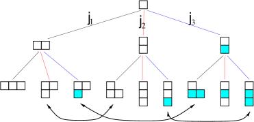
                           $$\stackrel{{\scriptstyle{\mathtt{P}}}}{{\leftrightarrow}} \stackrel{{\scriptstyle(13)}}{{\leftrightarrow}}$$   

Figure 9. All one-nation solution types up to rank-3, and all non-trivial ${\mathtt{P}}$-orbits.

(0.A.1) On a given solution $R\in{\mathsf{Match}}^{N}(2,2)$ the ${\mathtt{P}}$ action leaves the $a_{i}$s unchanged but interchanges the diagonal and skew-diagonal entries on all $A(i,j)$ simultaneously. On a germ this has the effect of simultaneously changing all ${\mathsf{f}}$ edges to $\underline{{\mathsf{f}}}$, ${\mathsf{a}}$ edges to $\underline{{\mathsf{a}}}$ and vice versa. It leaves the $/$ edges and the $0$ edges unchanged, so that the memberships of nations and counties are unchanged; but the order of counties in their nation is reversed.

For example consider the variety of solutions associated to the first diagram here:

 $$\stackrel{{\scriptstyle{\mathtt{P}}}}{{\leftrightarrow}} \stackrel{{\scriptstyle(13)}}{{\leftrightarrow}}$$   

From this diagram, for each point $(\alpha_{1},\beta_{1})$ in type space (a specific pair of complex numbers) we get the solution with $a_{1}=a_{2}=\alpha_{1}$, $a_{3}=\beta_{1}$ and so on. Applying ${\mathtt{P}}$ does not change the $a_{i}$s, so we have the middle diagram and still $(\alpha_{1},\beta_{1})$. Applying $(13)\in\Sigma_{3}$ takes the $a_{i}$s to $a_{1}=\beta_{1}$ and $a_{2}=a_{3}=\alpha_{1}$. This is the specific solution we would associate to $(\beta_{1},\alpha_{1})$ not $(\alpha_{1},\beta_{1})$ via the last diagram, but these are points in the same variety.

We see that starting in ${\mathfrak{T}}_{N}$ the action of ${\mathtt{P}}$ takes us out of the subset. But since ${\mathtt{P}}$ and $\Sigma_{N}$ actions commute we have an action of ${\mathtt{P}}$ on classes (represented by unfilled diagrams). Up to rank 3 the orbits are indicated in Fig.9.

Consider the varieties of solutions indicated by the following rank-4 one-nation diagrams:

           

The first is ${\mathsf{b}}({\mathsf{j}}(122))$, and the fifth for example is ${\mathsf{b}}({\mathsf{j}}(212))$. The fifth (also the seventh) is fixed under our extended transformation group ${\mathcal{G}}_{N}=\mathbb{Z}_{2}\times\Sigma_{N}$. However the fifth gives solutions that are conjugate, as matrices, to those from the first. Conjugation here can be achieved by a non-local permutation matrix in ${\mathsf{Match}}^{N}(2,2)$.

0.A.2. Signatures: Eigenvalues and isomorphism from a linear perspective

 

A signature is, roughly, the eigenvalue spectrum of the solution matrix for each solution type. Since the actual eigenvalues of a solution ${\mathsf{F}}(\sigma)$ come from the specific point on the variety, what we focus on here is the generic degeneracies rather than the values. Since the largest block matrix in $F(\sigma)$ is $2\times 2$, we can compute the generic degeneracies for each variety (indeed in principle we can compute a Jordan form including all points). We will give the degeneracies as an unordered list, and hence as a partition of $N^{2}$. Notationally we may write $\boldsymbol{\alpha}\rightarrow\omega(\boldsymbol{\alpha})$ if $\omega(\boldsymbol{\alpha})$ is the list of degeneracies for configuration $\boldsymbol{\alpha}$.

It is straightforward to work out eigenvalues and multiplicities for a specific class of solutions — i.e. for $F(\sigma)$. As noted, if two eigenvalue spectrums do not agree, then the solutions cannot be isomorphic. But even when they do agree, they may not be isomorphic.

Rank-1 is trivial: we write $\square\rightarrow(1)$ to denote that the trivial variety $\square$ has solutions with a single eigenvalue with degeneracy 1. Rank-2 is straightforward. Our types $0,{\mathsf{f}},{\mathsf{a}},/$ are:
$\square\!\square\rightarrow(4)$,  $\includegraphics[width=7.14183pt]{xfig/tree123Pa2.eps}\rightarrow(3,1)$,  $\includegraphics[width=7.14183pt]{xfig/tree123Pa3.eps}\rightarrow(2,2)$,  $\square\;\square\rightarrow(1^{4})$.
Let us note in passing: (1) Type ${\mathsf{f}}$ has two eigenvalues with degeneracies (3,1), corresponding to the classical $U_{q}sl_{2}$ symmetry: $2\otimes 2=3\oplus 1$ (sometimes written $\square\otimes\square=\square\!\square\oplus\emptyset$ [Dri85, Jim86]).
(2) Type $/$ can be specialised to $\alpha_{1}=\alpha_{2}$ whereupon (up to the trivial overall factor) we recover the representations given in [Mar91, §12.1.1] (cf. the Birman–Murakami–Wenzl algebra).

In general $\omega(\boldsymbol{\alpha})$ ‘factorises’ into a contribution $\phi(\boldsymbol{\alpha})$ from $/$ edges and a contribution $\nu_{i}(\boldsymbol{\alpha})$ from each nation: $\omega(\boldsymbol{\alpha})=\phi(\boldsymbol{\alpha})\prod_{i}\nu_{i}(\boldsymbol{\alpha})$.

(0.A.2) The contribution of eigenvalues of the form $\pm\mu_{ij}$ from $/$ edges is given in general by the following. Let nations of a solution $\boldsymbol{\alpha}$ be indexed by some ordered set $I=I(\boldsymbol{\alpha})$; and for $i\in I$ let $N_{i}=|p_{i}|$ denote the size of nation $i$. Then the part of the signature of solution $\boldsymbol{\alpha}$ coming from edges between nations is

$$\phi(\boldsymbol{\alpha})\;=\prod_{i<j\in I}(N_{i}N_{j},N_{i}N_{j})$$

— that is, there are $N_{i}N_{j}$ eigenalues $\pm\mu_{ij}$. For example, If $\lambda=\square\!\square\;\;\square$ then we have just $(2,2)$ from these edges. The number of free parameters $\mu_{ij}$ in the variety coming from this part of the matrix is ${{|I|}\choose{2}}$.

Meanwhile each nation $i$ contributes (one or) two eigenvalues, with multiplicities given as follows. Let $\#_{i}0$ denote the number of 0 edges. Let set $J_{i}$ index the counties, i.e. the elements of $q|p_{i}$. Then $\#_{i}0\;=\;\sum_{j\in J_{i}}{{|q_{j}|}\choose{2}}$. Let $s_{2}(i)$ denote the set of blue (colour 2) vertices. We have

$$\nu_{i}(\boldsymbol{\alpha})=({{N_{i}}\choose{2}}+\#_{i}0+|s_{1}(i)|,{{N_{i}}\choose{2}}-\#_{i}0+|s_{2}(i)|).$$ (21)

Note: (i) That this does not depend on the order on counties. (ii) That each one-nation representation is (up to an elementary rescaling) a representation of some Hecke algebra.

In practice we may notate $\omega(\boldsymbol{\alpha})$ as $(\nu_{1};\nu_{2};...;\nu_{|I|}:\phi)$.  Now consider rank-3.

(0.A.3) We start with $\square\;\square\;\square=///$ in $N=3$ as in Lemma 5.4. Here there are (up to) 9 distinct eigenvalues ($a_{1},a_{2},a_{3},\pm\mu,\pm\nu,\pm\lambda$), each of multiplicity 1; given by 6 free parameters ($a_{1},a_{2},a_{3},\mu,\nu,\lambda$), as shown. We record this as the ‘signature’ $(1^{9})=(1;1;1:1,1,1,1,1,1)$.

$$\lx@xy@svg{\hbox{\raise 0.0pt\hbox{\kern 16.76518pt\hbox{\ignorespaces\ignorespaces\ignorespaces\hbox{\vtop{\kern 0.0pt\offinterlineskip\halign{\entry@#!@&&\entry@@#!@\cr&\\&&\crcr}}}\ignorespaces{\hbox{\kern-3.0pt\raise 0.0pt\hbox{\hbox{\kern 0.0pt\raise 0.0pt\hbox{\hbox{\kern 3.0pt\raise 0.0pt\hbox{$\textstyle{}$}}}}}}}{\hbox{\kern 40.76518pt\raise 0.0pt\hbox{\hbox{\kern 0.0pt\raise 0.0pt\hbox{\hbox{\kern 3.0pt\raise 0.0pt\hbox{$\textstyle{{a_{2}}_{{\color[rgb]{1,.5,0}\tiny2⃝}}\ignorespaces\ignorespaces\ignorespaces\ignorespaces\ignorespaces}$}}}}}}}\ignorespaces\ignorespaces\ignorespaces{}\ignorespaces\ignorespaces{\hbox{\lx@xy@drawline@}}\ignorespaces{\hbox{\kern 76.44661pt\raise-19.42776pt\hbox{\hbox{\kern 0.0pt\raise-1.75pt\hbox{$\scriptstyle{\;\;\;\;/_{\pm\nu}}$}}}}}\ignorespaces\ignorespaces{\hbox{\lx@xy@drawline@}}\ignorespaces{\hbox{\kern 104.25224pt\raise-31.55pt\hbox{\hbox{\kern 0.0pt\raise 0.0pt\hbox{\lx@xy@tip{1}\lx@xy@tip{-1}}}}}}\ignorespaces\ignorespaces{\hbox{\lx@xy@drawline@}}\ignorespaces{\hbox{\lx@xy@drawline@}}{\hbox{\kern-16.76518pt\raise-38.85555pt\hbox{\hbox{\kern 0.0pt\raise 0.0pt\hbox{\hbox{\kern 3.0pt\raise 0.0pt\hbox{$\textstyle{{{a_{1}}}^{{\color[rgb]{1,.5,0}\tiny1⃝}}\ignorespaces\ignorespaces\ignorespaces\ignorespaces\ignorespaces\ignorespaces\ignorespaces\ignorespaces\ignorespaces\ignorespaces}$}}}}}}}\ignorespaces\ignorespaces\ignorespaces{}\ignorespaces\ignorespaces{\hbox{\lx@xy@drawline@}}\ignorespaces{\hbox{\kern 18.69911pt\raise-19.42778pt\hbox{\hbox{\kern 0.0pt\raise-1.65279pt\hbox{$\scriptstyle{\;\;\;\;/_{\pm\mu}}$}}}}}\ignorespaces\ignorespaces{\hbox{\lx@xy@drawline@}}\ignorespaces{\hbox{\kern 47.90732pt\raise-6.5pt\hbox{\hbox{\kern 0.0pt\raise 0.0pt\hbox{\lx@xy@tip{1}\lx@xy@tip{-1}}}}}}\ignorespaces\ignorespaces{\hbox{\lx@xy@drawline@}}\ignorespaces{\hbox{\lx@xy@drawline@}}\ignorespaces\ignorespaces\ignorespaces\ignorespaces{}{\hbox{\lx@xy@droprule}}\ignorespaces{\hbox{\kern 50.28043pt\raise-38.85555pt\hbox{\hbox{\kern 0.0pt\raise-1.75pt\hbox{$\scriptstyle{\;/_{\pm\lambda}\;}$}}}}}{\hbox{\lx@xy@droprule}}\ignorespaces{\hbox{\kern 98.29555pt\raise-38.85555pt\hbox{\hbox{\kern 0.0pt\raise 0.0pt\hbox{\lx@xy@tip{1}\lx@xy@tip{-1}}}}}}{\hbox{\lx@xy@droprule}}{\hbox{\lx@xy@droprule}}{\hbox{\kern 54.53036pt\raise-38.85555pt\hbox{\hbox{\kern 0.0pt\raise 0.0pt\hbox{\hbox{\kern 3.0pt\raise 0.0pt\hbox{$\textstyle{}$}}}}}}}{\hbox{\kern 98.29555pt\raise-38.85555pt\hbox{\hbox{\kern 0.0pt\raise 0.0pt\hbox{\hbox{\kern 3.0pt\raise 0.0pt\hbox{$\textstyle{{}_{{\color[rgb]{1,.5,0}\tiny3⃝}}{a_{3}}}$}}}}}}}\ignorespaces}}}}\ignorespaces\hskip 7.22743ptsignature:\;(1^{9}),6 \textstyle{{a_{2}}_{{\color[rgb]{1,.5,0}\tiny2⃝}}\ignorespaces\ignorespaces\ignorespaces\ignorespaces\ignorespaces} \scriptstyle{\;\;\;\;/_{\pm\nu}} \textstyle{{{a_{1}}}^{{\color[rgb]{1,.5,0}\tiny1⃝}}\ignorespaces\ignorespaces\ignorespaces\ignorespaces\ignorespaces\ignorespaces\ignorespaces\ignorespaces\ignorespaces\ignorespaces} \scriptstyle{\;\;\;\;/_{\pm\mu}} \scriptstyle{\;/_{\pm\lambda}\;} \textstyle{{}_{{\color[rgb]{1,.5,0}\tiny3⃝}}{a_{3}}} \textstyle{{a_{2}}_{{\color[rgb]{1,.5,0}\tiny2⃝}}\ignorespaces\ignorespaces\ignorespaces\ignorespaces\ignorespaces} \scriptstyle{\;\;\;\;/_{\pm\nu}} \textstyle{{{a_{1}}}^{{\color[rgb]{1,.5,0}\tiny1⃝}}\ignorespaces\ignorespaces\ignorespaces\ignorespaces\ignorespaces\ignorespaces\ignorespaces\ignorespaces\ignorespaces\ignorespaces} \scriptstyle{\;\;\;\;/_{\pm\mu}} \scriptstyle{\;/_{\pm\lambda}\;} \textstyle{{}_{{\color[rgb]{1,.5,0}\tiny3⃝}}{a_{3}}}$$

(0.A.4) For $\includegraphics[width=7.14183pt]{xfig/tree123Pa2.eps}\;\square$, so for example $//{\mathsf{f}}$ as in Lem.5.5, there is 1 eigenvalue of multiplicity 3; 2 eigenvalues of multiplicity 2; and there are 2 eigenvalues of multiplicity 1, all given by 4 parameters. Note that there is a variable $\beta$ associated to the ${\mathsf{f}}$ edge which does not manifest elsewhere. Note also that the object cannot be diagonalised over the ground ring, or more specifically it would have a non-trivial Jordan block in the specialisation $a_{1}=\beta$.

(0.A.5) Altogether for $N=3$ (here giving just the degeneracies, for a ${\mathcal{G}}_{N}$-transversal cf. Prop.5):

$\!\!\!\begin{array}[]{c}\square\!\square\!\square\\ =000\\ \rightarrow(9)\end{array}\!\!\!$

$\!\!\!\begin{array}[]{c}\includegraphics[width=14.51074pt]{xfig/tree123Pa13.eps}\\ 0{\mathsf{a}}{\mathsf{a}}\\ (6,3)\end{array}\!\!\!$

$\!\!\!\begin{array}[]{c}\includegraphics[width=14.51074pt]{xfig/tree123Pa12.eps}\\ 0ff\\ (7,2)\end{array}\!\!\!$

$\!\!\!\begin{array}[]{c}\includegraphics[width=7.14183pt]{xfig/tree123Pa32.eps}\\ afa\\ (5,4)\end{array}\!\!\!$

$\!\!\!\begin{array}[]{c}\includegraphics[width=7.14183pt]{xfig/tree123Pa23.eps}\\ faa\\ (5,4)\end{array}\!\!\!$

$\!\!\!\begin{array}[]{c}\includegraphics[width=7.14183pt]{xfig/tree123Pa22.eps}\\ fff\\ (6,3)\end{array}\!\!\!$

$\!\!\!\begin{array}[]{c}\square\!\square\;\square\\ 0//\\ (4;1:2,2)\end{array}\!\!\!$

$\!\!\!\begin{array}[]{c}\includegraphics[width=7.14183pt]{xfig/tree123Pa2.eps}\;\square\\ f//\\ (3,1;1:2,2)\end{array}\!\!\!$

$\!\!\!\begin{array}[]{c}\includegraphics[width=7.14183pt]{xfig/tree123Pa3.eps}\;\square\\ a//\\ (2,2;1:2,2)\end{array}\!\!\!$

$\!\!\!\begin{array}[]{c}\square\;\square\;\square\\ ///\\ (1;1;1:1^{6})\end{array}\!\!\!$

Notes: (i) In general $|{\mathfrak{T}}_{N}|=1,4,13,46,154,...$ is the Euler ‘forest’ transform of the one-nation sequence $3^{N-1}$ (cf. Fig.10). This is A104460 in [Slo21]. From the ${\mathtt{P}}$-orbits in Fig.9, the ${\mathcal{G}}_{N}$-transversal for $N=3$ here is 3 elements smaller than the $\Sigma_{N}$-transversal, thus ten entries.
(ii) The two (5,4) cases are related as per (0.A.2)(i), but are not related by our symmetries, but they are similar as matrices by a non-local conjugation.
(iii) The two (6,3) cases have different Jordan structure over the polynomial ring of indeterminates.

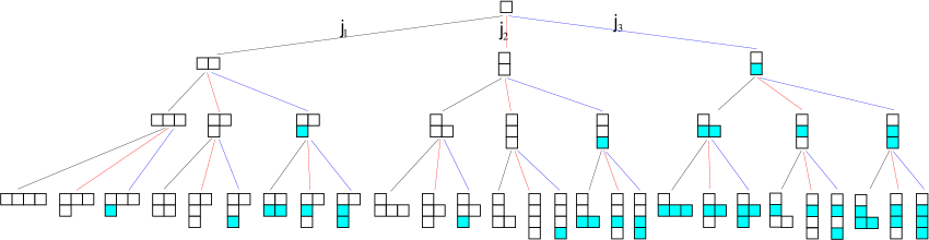
Figure 10. One-nation configurations up to rank-4.

(0.A.6) For $N=4$ the one-nation cases (cf. Fig.10, and taking account of (0.A.2)(i)) and some indicative multination cases are:

$\!\!\!\begin{array}[]{c}\square\!\square\!\square\!\square\\ \rightarrow(16)\end{array}\!\!\!$

$\!\!\!\begin{array}[]{c}\includegraphics[width=21.33955pt]{xfig/y000aaa.eps}\\ (12,4)\end{array}\!\!\!$

$\!\!\!\begin{array}[]{c}\includegraphics[width=21.33955pt]{xfig/y000fff.eps}\\ (13,3)\end{array}\!\!\!$

$\!\!\!\begin{array}[]{c}\includegraphics[width=14.22636pt]{xfig/y0aaaa0.eps}\\ {(8,8)}\end{array}\!\!\!$

$\!\!\!\begin{array}[]{c}\includegraphics[width=14.22636pt]{xfig/y0ffff0.eps}\\ (12,4)\end{array}\!\!\!$

$\!\!\!\begin{array}[]{c}\includegraphics[width=14.22636pt]{xfig/yaa0faa.eps}\\ (9,7)\end{array}\!\!\!$

$\!\!\!\begin{array}[]{c}\includegraphics[width=14.22636pt]{xfig/yaa0aff.eps}\\ (10,6)\end{array}\!\!\!$

$\!\!\!\begin{array}[]{c}\includegraphics[width=14.22636pt]{xfig/yff0aaa.eps}\\ (10,6)\end{array}\!\!\!$

$\!\!\!\begin{array}[]{c}\includegraphics[width=14.22636pt]{xfig/yff0fff.eps}\\ {(11,5)}\end{array}\!\!\!$

$\!\!\!\begin{array}[]{c}\includegraphics[width=7.68236pt]{xfig/yfaaaaf.eps}\\ (8,\;8)\end{array}\!\!\!$

$\!\!\!\begin{array}[]{c}\includegraphics[width=7.68236pt]{xfig/yfffaaa.eps}\\ (9,\;7)\end{array}\!\!\!$

$\!\!\!\begin{array}[]{c}\includegraphics[width=7.68236pt]{xfig/yffffff.eps}\\ (10,\;6)\end{array}\!\!\!$

$\!\!\!\begin{array}[]{c}\square\!\square\!\square\;\square\\ (9;1:3,3)\end{array}\!\!\!$

$\!\!\!\begin{array}[]{c}\includegraphics[width=14.51074pt]{xfig/tree123Pa12.eps}\;\square\\ (7,2;1:3,3)\end{array}\!\!\!$

$\!\!\!\begin{array}[]{c}\square\!\square\;\square\!\square\\ (4;4:4,4)\end{array}\!\!\!$

$\!\!\!\begin{array}[]{c}\includegraphics[width=7.82736pt]{xfig/tree123Pa2.eps}\;\square\!\square\\ (3,1;4:4,4)\end{array}\!\!\!$

$\!\!\!\begin{array}[]{c}\includegraphics[width=7.82736pt]{xfig/tree123Pa3.eps}\;\square\!\square\\ (2,2;4:4,4)\end{array}\!\!\!$

…

$\!\!\!\begin{array}[]{c}\square\;\square\;\square\;\square\\ (1;1;1;1:1^{12})\end{array}\!\!\!$

0.A.3. On ${\mathsf{Match}}^{N}$ representation theory

 

 

In Artinian representation theory the natural notions of isomorphism and of additivity ‘agree’ with each other so that the classification is canonical. In our case there are layers of naturality and the tie-up is more complex (cf. [MM14, RW18] etc).

Given a representation $F$ on ${\mathsf{Match}}^{N}$ (we will just say a representation on $N$) there is, via Lemma 3.7III, a sense in which each subset $S\subseteq\underline{N}$ gives a subrepresentation $F|_{S}$. I.e. every subset gives an invariant subset, with a ‘complementary’ representation on $\underline{N}\setminus S$. However, there is also a novel form of additivity — an ‘adjoint’ to this ‘restriction’. It does not make immediate sense to talk of adding reprentations (as in direct sums), or in particular of resumming the representations on $S$ and $\underline{N}\setminus S$. However there is an additive property:   Given representations on $N$ and $M$ we obtain a representation on $N\sqcup M\hookrightarrow N+M$ by completing the $K_{N}\sqcup K_{M}$ subgraph of the complete graph $K_{N\sqcup M}$ with $/$ edges. (Proof: every new triangle contains two $/$s, and now use the second row of configurations from Prop.5, via Lemma 3.13, noting that the orientation of $/$ edges — the relative placement of the singleton vertex of the three — does not here affect the validity of the solution.)   This addition is substantially different from direct sum — for one thing these edges carry parameters so this gives not a single isomorphism class of representations in the classical sense but a variety. Let us write $F\oslash G$ for the variety of representations constructed from $F$ on $N$ and $G$ on $M$ say — noting that many choices are needed to select a concrete representation from this variety. What is not true in general is that $F|_{S}\oslash F|_{\underline{N}\setminus S}\ni F$. For this to hold, we require that $S$ is a union of nations of $F$ — so that a nation is a kind of irreducible representation.

In this sense classifying representations first by classifying single-nation representations and then giving composition multiplicities of general representations in terms of such ‘irreducible’ content is roughly in analogy with Jordan–Holder.

Appendix 0.B On rectanguloid/X-equivalence and Lemma 3.13

(0.B.1) Explicit proof of Lemma 3.13. Observe from Theorem 3.12 that the constraint equations are satisfied by the substitutions

$$\left(\begin{array}[]{cc}a_{ij}&b_{ij}\\ c_{ij}&d_{ij}\end{array}\right)\leadsto\;\left(\begin{array}[]{cc}a_{ij}&x_{ij}b_{ij}\\ c_{ij}/x_{ij}&d_{ij}\end{array}\right)$$

(the upshot of a conjugation by $X\in{\mathsf{Match}}^{N}(2,2)$ as in the Lemma) given that they are satisfied by ${\mathsf{F}}(\sigma)$, because the entries $b_{ij},c_{ij}$, if appearing with non-zero coefficient, appear as $b_{ij}c_{ij}$, or else as an overall factor.     The equivalence relation property follows by construction. ∎

We note that neither general solutions to the Yang-Baxter equation, nor spin-chain representations of other categories, are stable under conjugation by non-local diagonal matrices. — Meaning that a solution ${\mathsf{F}}:{\mathsf{B}}\rightarrow{\mathsf{Mat}}^{N}$ given in the form ${\mathsf{F}}(\sigma)$ is not necessarily taken to a solution unless $X$ of the form $X=\mu\otimes\mu$ (i.e. unless ${\mathsf{F}}\leadsto{\mathsf{F}}\circ{\mathsf{C}}^{\mu}$).

(0.B.2) Formally a conjugating functor associates a suitable invertible matrix $\mu^{(m)}$ to each object $m$, and transforms morphism according to: $f\mapsto\mu^{(s(f))}f\overline{\mu}^{(t(f))}$, where $s,t$ are the source and tail functions. This obviously behaves well under category composition (so gives a functor), but not necessarily under monoidal composition (so does not give a monoidal functor in general). A necessary condition is that it acts on the whiskerings of $F(\sigma)\in{\mathsf{Match}}^{N}(2,2)$ like $\mu^{(3)}F(\sigma)\otimes 1\overline{\mu}^{(3)}=\mu^{(2)}F(\sigma)\overline{\mu}^{(2)}\otimes 1$ and $\mu^{(3)}1\otimes F(\sigma)\overline{\mu}^{(3)}=1\otimes\mu^{(2)}F(\sigma)\overline{\mu}^{(2)}$. This of course holds if $\mu^{(m)}=\mu^{\otimes m}$ as before - the ‘local’ solution; but we are looking for something more. An interesting question is if this can be made to work with some degree of generality, or if the only possibilities arise when we pass all the way to the constraints coming from the YBE.
Observe that a conjugating functor, where defined, is determined by its action on a generating set of morphisms, and hence on the $\overline{\mu}^{(m)}$’s for objects in their sources and tails (so in our case by $\overline{\mu}^{(2)}$ — the $X$ of the X Lemma). It is an interesting question then, in our case, given a valid $\overline{\mu}^{(2)}$, what is $\overline{\mu}^{(m)}$? Our setup is a nice playground for this. Explicitly, taking the in-line form of $A\in{\mathsf{Match}}^{N}(2,2)$ as in (16)

$${\underline{\alpha}}(A)=(a_{1},a_{2},\ldots,a_{N},\left(\begin{array}[]{cc}a_{12}&b_{12}\\ c_{12}&d_{12}\end{array}\right),\ldots,\left(\begin{array}[]{cc}a_{ij}&b_{ij}\\ c_{ij}&d_{ij}\end{array}\right),\ldots),$$

conjugation by an invertible diagonal matrix defined by $X(\mathfrak{e}_{i}\otimes\mathfrak{e}_{j})=y_{ij}(\mathfrak{e}_{i}\otimes\mathfrak{e}_{j})$ gives

$${\underline{\alpha}}(XAX^{-1})=(a_{1},a_{2},\ldots,a_{N},\left(\begin{array}[]{cc}a_{12}&x_{12}b_{12}\\ c_{12}/x_{12}&d_{12}\end{array}\right),\ldots,\left(\begin{array}[]{cc}a_{ij}&x_{ij}b_{ij}\\ c_{ij}/x_{ij}&d_{ij}\end{array}\right),\ldots)$$ (22)

where $x_{ij}:=\frac{y_{ij}}{y_{ji}}$ for $i<j$.

The local case $X=\mu\otimes\mu$, with $\mu\mathfrak{e}_{i}=y_{i}\mathfrak{e}_{i}$ say, gives $y_{ij}=y_{i}y_{j}$ and hence lies in the center of ${\mathsf{Match}}^{N}(2,2)$ and acts trivially. By virtue of the Lemma (i.e. for the case of ${\mathsf{B}}$ and possibly not in general) we have also the decomposable case $X=\mu\otimes\nu$, with $\nu\mathfrak{e}_{i}=z_{i}\mathfrak{e}_{i}$ say; and the entangled case. Just to see if it has interesting special features, let us consider the case $X=\mu\otimes\nu$. This gives $y_{ij}=y_{i}z_{j}$ and hence $x_{ij}=\frac{y_{i}z_{j}}{y_{j}z_{i}}$. For $N=3$ we have $x_{12}=\frac{y_{1}}{z_{1}}\frac{z_{2}}{y_{2}}$, $x_{13}=\frac{y_{1}}{z_{1}}\frac{z_{3}}{y_{3}}$, $x_{23}=\frac{y_{2}}{z_{2}}\frac{z_{3}}{y_{3}}$. This is clearly not generic. An interesting question is whether X-equivalence can be realised ‘functorially’ (in particular via a conjugating functor) in general.

Appendix 0.C Details for proof of Theorem 4.13

0.C.1. On further properties of $\Sigma_{N}$-orbits of solutions

 

(0.C.1) 6-rule: If an oriented chain of two edges is signed with the same sign in a solution ${\mathsf{F}}(\sigma)$ then the ‘long’ edge completing the triangle is signed with the same sign. — To see this check the 9-rule list from 5 and the orbit of +++ in Table 1.
(This is called 6-rule since it reduces the number of possible edge $\pm$-colourings of a triangle from eight to six. It also reduces the number of $\pm 0$-colourings.)

Lemma 0.C.2.

Every $\Sigma_{N}$ orbit of solutions in ${\mathsf{R}}({\mathfrak{S}}^{\mathbb{C}}_{N})$ contains an element with no $-$-orientation.
Furthermore, in such a   ‘$-$-free’ configuration the elements of a 0-part (a county) are clustered with respect to the natural order in their nation, i.e. they are consecutive.

Proof.

First we note that the claim holds if it holds for 1-nation solutions, since there are perms that act non-trivially only on a single nation and the $/$-edges out of that nation, restricting to a complete set of perms on that nation. So now consider a single nation. We work by induction on $N$. The claim is true for $N<4$ by inspection of our explicit solution sets. Suppose true at level-$N$ and consider $N+1$. WLOG by inductive assumption consider a configuration with all (signed) edges $+$ between vertices $1,2,\cdots,N$ (any non-signed edges are 0). Consider what configurations of edges to vertex $N+1$ are allowed here. Neglecting cases with 0s on the edges to $N+1$ for a moment we have, say, as on the left here:

     

By the 6-rule, if the $i$ to $N+1$ edge is + then, since the $i-1$ to $i$ edge is +, the $i-1$ to $N+1$ edge is also +. Indeed this is also forced in the case where the $i-1$ to $i$ edge is 0. Thus there are $N$ possible configurations of form $++...+--...-$ (NB all these arrows point to $N+1$). The $i$-th of these configurations is taken to $+++...+$ by the perm $(i\;i\!\!+\!\!1\cdots N)$, so we are done in these cases. In case of 0 on a long edge $i$ to $N+1$, the edges $j$ ($j<i$) to $i$ and $j$ to $N+1$ must be the same, so these edges satisfy the no-$-$ claim. Thus it remains only to address the edges after the last 0. Suppose this last 0 is $i$ to $N+1$. The edges $k$ to $N+1$ with $k>i$ will all be opposite to the corresponding $i$ to $k$ edge (which is either + or 0), so either $-$ or 0. Now apply the perm $(i\;N\!+\!1)$. This has the effect of making the $N+1$ vertex the ‘new’ $i$ vertex and incrementing $i$ et seq. Thus all the edges that were $k$ to $N+1$ are reversed, so all the $-$s become +, while the relative positions of all other vertices are preserved, so signs do not change — i.e. they remain $-$-free.

The second claim follows from the 6-rule: given $ij$ and $jk$ are + then $ik$ is +, so not 0. ∎

(0.C.3) Note from (4.2) that recipe ${\mathsf{R}}$ assigns a configuration to a $K_{2}$ subgraph dependent on the relative rather than absolute values of the vertex labels.
In this sense an inclusion $\psi:\underline{M}\hookrightarrow\underline{N}$ as in 3.7III that is order preserving induces a ‘stronger’ equivalence between a configuration on $M$ and the restriction of a configuration on $N$ to the image $\psi(\underline{M})$ than for a generic inclusion. Such an order-preserved image is essentially identical - changed only in being moved.
Similarly, for a bijection $\psi:\underline{N}\stackrel{{\scriptstyle\sim}}{{\rightarrow}}\underline{N}$ we may partition the domain (not necessarily uniquely) into a set $p$ of subsets on each of which $\psi$ is order-preserving (e.g. the set of singleton subsets is trivially preserved by any $\psi$) and then $\psi$ moves these subsets ‘parallel-ly’ around in $\underline{N}$ and the image of each under ${\mathsf{R}}$ gives an identical configuration. Meanwhile, although the whole of the image under $\psi$ of a solution is another solution, while it is isomorphic, it is generally differently configured on edges between parts of $p$.

(0.C.4) On the proof of Theorem 4.13. The Theorem asserts that every point on every variety of solutions may be obtained by applying ${\mathsf{R}}$ from (4.2) to the image of some point in ${\mathfrak{T}}_{N}^{\mathbb{C}}$ under some $w\in\Sigma_{N}$. This begs the question of how $\Sigma_{N}$ acts on ${\mathfrak{S}}_{N}^{\mathbb{C}}$. Let $w\in\Sigma_{N}$ act on ${\mathfrak{S}}_{N}$ by permuting vertex labels. Ignoring parameters for a moment it will be clear that ${\mathfrak{T}}_{N}$ is a transversal of $\Sigma_{N}$-orbits of ${\mathfrak{S}}_{N}$. Thus we will be done if we can show that there is an action on ${\mathfrak{S}}_{N}^{\mathbb{C}}$ that reduces to this, and such that the square:

(23)

(where the action of $w$ on the right is via the functor in $\mathfrak{Func}({\mathsf{Match}}^{N},{\mathsf{Match}}^{N})$) commutes up to trivial movement on the variety.

Figure 11 illustrates the action of $\Sigma_{N}$ on an example solution. The change expressed at the level of ${\mathfrak{S}}_{N}^{\mathbb{C}}$ is

$$\begin{array}[]{c}\includegraphics[width=11.66573pt]{xfig/young111-123.eps}\\ {}^{\alpha_{1}}\\ {}^{\beta_{1}}\end{array}\hskip 5.97527pt\begin{array}[]{c}\includegraphics[width=11.66573pt]{xfig/young11-45.eps}\\ {}^{\alpha_{2}}\\ {}^{\beta_{2}}\end{array}\hskip 5.97527pt\begin{array}[]{c}\includegraphics[width=11.66573pt]{xfig/young1-6.eps}\\ {}^{\alpha_{3}}\end{array}\hskip 15.17719pt\raisebox{18.55098pt}{$\;\;\;\;\stackrel{{\scriptstyle(34)}}{{\leadsto}}\;\;\;\;$}\hskip 15.17719pt\begin{array}[]{c}\includegraphics[width=11.66573pt]{xfig/young111-124.eps}\\ {}^{\alpha_{1}}\\ {}^{\beta_{1}}\end{array}\hskip 5.97527pt\begin{array}[]{c}\includegraphics[width=11.66573pt]{xfig/young11-35.eps}\\ {}^{\alpha_{2}}\\ {}^{\beta_{2}}\end{array}\hskip 5.97527pt\begin{array}[]{c}\includegraphics[width=11.66573pt]{xfig/young1-6.eps}\\ {}^{\alpha_{3}}\end{array}$$

(NB the specific names $\alpha_{1}$ etc used here to represent parameter values are not portable in general — only which are ‘related’ and which are independent. To give a point in type-space we would need to order the component nations.) Ignoring parameters, i.e. at the level of ${\mathfrak{S}}_{N}$, this is of course the same as the direct action. Now observe that up to ‘signs’ the collection of triangle configurations are simply rearranged on $K_{N}$ by the permutation. For example the fff triangle moves from vertices 123 to 124 under the action of $(34)\in\Sigma_{N}$. (In the illustrated case there are no sign changes since 3,4 are adjacent and the 34-edge is $/$-decorated.) Since triangles collectively are at most rearranged up to signs, the relationships of $\alpha_{i}$ and $\beta_{i}$ parameters are preserved, so the open conditions defining the type-space are preserved.

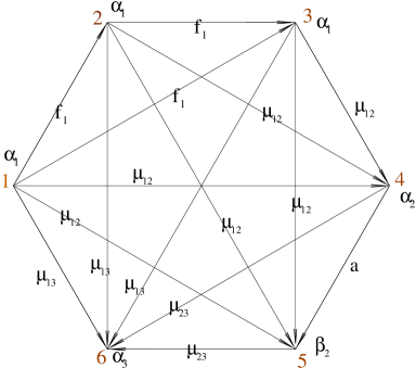
$$\;\;\;\;\stackrel{{\scriptstyle(34)}}{{\leadsto}}\;\;\;\;$$

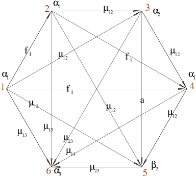
Figure 11. Action of $(34)\in\Sigma_{N}$ on a solution with $N=6$ and three nations. On $/$ edges we simply give (names of form $\mu_{ij}$ for) the parameters. We write ${\mathsf{f}}_{1}$ for ${\mathsf{f}}_{\beta_{1}}$ to avoid clutter.

0.C.2. 2-coloured composition combinatorics

 

In light of Lemma 0.C.2 we can characterise orbits of representations in terms of suitable partitioned integer compositions — describing nations in an element of the $-$-free transversal of ${\mathfrak{S}}_{N}$. Next we develop useful facility with these objects, and match to §4.

(0.C.5) If $\lambda=\lambda_{1}\lambda_{2}\cdots\lambda_{L}$ is a composition then we write $\Gamma_{\lambda}$ for the set

$$\Gamma_{\lambda}=\times_{i=1}^{L}\Gamma_{\lambda_{i}}$$

Example: $\Gamma_{22}=\{(11,11),(11,2),(2,11),(2,2)\}$. We may write $\mu\models\lambda$ for $\mu\in\Gamma_{\lambda}$.
If $\lambda$ is a partition we write $\Gamma^{\prime}_{\lambda}$ for the subset of $\Gamma_{\lambda}$ of multicompositions $\mu$ such that if there are parts of $\lambda$ of tied order then their compositions appear in $\mu$ in (weak) lex order.
Example $\Gamma^{\prime}_{22}=\{(11,11),(11,2),(2,2)\}$. We may write $\mu\models^{\!\!\!\!\!\circ}\lambda$ for $\mu\in\Gamma^{\prime}_{\lambda}$.

(0.C.6) We can regard a composition $\lambda\in\Gamma_{N}$ as a set — of ordered parts — thus $\Gamma_{5}\ni\lambda=1+3+1=\{(1,1),(3,2),(1,3)\}$, say. Then ${\mathsf{P}}_{2}(\lambda)$ is the set of two-part partitions of the set of parts. Thus $\Gamma^{2}_{N}=\bigcup_{\lambda\in\Gamma_{M}}{\mathsf{P}}_{2}(\lambda).$
We can think of an element of $\Gamma^{2}_{N}$ either just as the 2-part partition, $s$ say, or as the pair $(\lambda,s)$, where $\lambda$ is the underlying composition (which can anyway be recovered from $s$).

(0.C.7) The following is simply a diagram-free recasting of the ${\mathsf{j}}$-function machinery from 4.2.
Let $\lambda=\lambda_{1}\lambda_{2}\cdots\lambda_{L}\in\Gamma_{N}$ be a non-empty composition. We define

$$\gamma^{l}(\lambda)=\lambda_{1}\lambda_{2}\cdots(\lambda_{L}+1)\hskip 28.45274pt\mbox{ and }\hskip 28.45274pt\gamma^{r}(\lambda)=\lambda_{1}\lambda_{2}\cdots\lambda_{L}1.$$

Observe that both $\gamma^{l}$ and $\gamma^{r}$ define injective functions from $\Gamma_{N}$ to $\Gamma_{N+1}$.
Similarly for $(\lambda,s)\in\Gamma^{2}_{N}$ define $\gamma^{l}(\lambda,s)$ as above with $(\lambda_{L}+1)$ in the same part of the 2-part partition as $\lambda_{L}$ was; and define $\gamma^{r}_{0}(\lambda,s)$ such that the added 1 is not in the same part of $s$ as $\lambda_{1}$, and $\gamma^{r}_{1}(\lambda,s)$ such that the added 1 is in the same part of $s$ as $\lambda_{1}$. Again observe that these functions are injective.

(0.C.8) The first part of the following is well known; the second part not so.
Proposition. (a) We have that $\gamma^{l}(\Gamma_{N})\cap\gamma^{r}(\Gamma_{N})=\emptyset$ and $\gamma^{l}(\Gamma_{N})\cup\gamma^{r}(\Gamma_{N})=\Gamma_{N+1}$. Thus in particular $|\Gamma_{N}|=2^{N-1}$.
(b) We have that $\gamma^{l}(\Gamma^{2}_{N}),\gamma^{r}_{0}(\Gamma^{2}_{N}),\gamma^{r}_{1}(\Gamma^{2}_{N})$ are disjoint, and $\gamma^{l}(\Gamma^{2}_{N})\cup\gamma^{r}_{0}(\Gamma^{2}_{N})\cup\gamma^{r}_{1}(\Gamma^{2}_{N})=\Gamma^{2}_{N+1}$. Thus in particular

$$|\Gamma^{2}_{N}|=3^{N-1}$$

Proof. (a) Disjointness is clear. For completeness note that every composition either ends in 1 or does not; and that in the former case it lies in $\gamma^{r}(\Gamma_{N})$ (indeed $\gamma^{r}$ has an inverse on the subset ending in 1), and in the latter in $\gamma^{l}(\Gamma_{N})$.
(b) The argument for (a) extends straightforwardly. The three subsets of $\Gamma^{2}_{N+1}$ to consider here are elements whose composition ends in 1 and this is not in the same part of $s$ as $\lambda_{1}$; elements whose composition ends in 1 and this is in the same part of $s$ as $\lambda_{1}$; and elements whose composition does not end in 1. ∎

(0.C.9) Given an integer partition, or indeed a composition, $\lambda=(\lambda_{1},\lambda_{2},...,\lambda_{m})$ of $N$ we have a partition of $\underline{N}=\{1,2,...,N\}$ into ‘nations’:

$${\mathsf{p}}_{\Lambda}(\lambda)=\{\{1,2,...,\lambda_{1}\},\{\lambda_{1}+1,\lambda_{1}+2,...,\lambda_{1}+\lambda_{2}\},\hskip 119.24506pt$$

$$\hskip 46.97505pt\{\lambda_{1}+\lambda_{2}+1,\lambda_{1}+\lambda_{2}+2,...,\lambda_{1}+\lambda_{2}+\lambda_{3}\},...,\{\left(\sum_{i=1}^{m-1}\lambda_{i}\right)+1,...,N\}\}$$

0.C.3. Symmetry orbits and transversals of solutions

 

(0.C.10) Our action of $\Sigma_{N}$ can be used to take any solution ${\mathsf{F}}$ to a representative with, say, largest nations first; and then at fixed nation size to lex order on compositions, so that all nations with composition $\lambda$ come before all with composition $\lambda^{\prime}>\lambda$.

(0.C.11) Proposition. A classification of the $\Sigma_{M}$-orbits of varieties of single-nation representations on $M$ say is given by $\Gamma_{M}^{2}$ — for $(\gamma,s)\in\Gamma_{M}^{2}$ the vertices in the two parts of $s$ are assigned the $\alpha$ and $\beta$ parameter respectively (e.g. $\Gamma_{2}^{2}=\{(2,\{\{1,2\}\}),\;(1+1,\{\{1\},\{2\}\}),\;(1+1,\{\{1,2\}\})\}$ corresponds to the set of edge labels $\{0,\mathsf{a},\mathsf{f}\}$).
Proof. This follows from Lemma 0.C.2 (or from our composition diagram construction and ${\mathsf{R}}$). ∎

(0.C.12) A classification of orbits of varieties of representations on $N$ is then by multiplicities $f\in\hom(\sqcup_{M\in{\mathbb{N}}}\Gamma_{M}^{2},{\mathbb{N}}_{0})$ such that the total degree is $N$, as in the Theorem. Combinatorics for this follows immediately from our Proposition 0.C.2(b) and the classical construction of multiset sequences (see for example [SP95, FS09] for the Euler transform).

Appendix 0.D Useful examples and schematics

(0.D.1) Each of our 2-coloured composition tableau $\lambda\in{\mathfrak{S}}_{N}$ yields a decoration of the vertices and edges of $K_{N}$, and hence a variety of functors via ${\mathsf{R}}$. To see the consistency of the construction, as in 6.3, we may firstly visualise the clustering of vertices into counties and nations as in Fig.12.

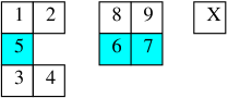
      $$\leadsto$$

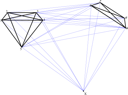
Figure 12. Geometric complete graph from a multiset of 2-coloured compositions.

Then all ‘long’ edges between nations $i,j$ get a $\mu_{ij}$ decoration; and ‘short’ edges a 0 (parameter inherited from vertices). (For remaining intranation edges see e.g. Fig.7.)

(0.D.2) Here we consider the $(p,q,\rho,s)$ form of ${\mathfrak{S}}_{N}$ as in 4.2. Given a finite set $S$ then $Perm(S)$ is the set of total orders of the elements, i.e. $Perm(S)=Hom^{iso}(S,\underline{|S|})$, the set of isomorphisms (although we express elements simply by giving the order).
If $p<q$ as in 4.2 et seq then $Perm_{p}(q)$ denotes the set of total orderings of the elements of $q$ in each $p_{i}$ (counties in each nation) without imposing an overall total order:

$$Perm_{p}(q)=\prod_{p_{i}\in p}Perm(q|p_{i})$$

Example:     $Perm_{\{\{1\},\{2,3\}\}}(\{\{1\},\{2\},\{3\}\})=\{\{(\{1\}),(\{2\},\{3\})\},\{(\{1\}),(\{3\},\{2\})\}\}$.
Finally, ${\mathsf{P}}_{2}(q/p)=\prod_{p_{i}\in p}{\mathsf{P}}_{2}(q|p_{i})\;$ — the set of partitionings of counties of each nation into at most two parts. Example: ${\mathsf{P}}_{2}(\{\{1\},\{2\},\{3\},\{4\}\}/\{\{1,2\},\{3,4\}\})={\mathsf{P}}_{2}(\{\{1\},\{2\}\})\prod{\mathsf{P}}_{2}(\{\{3\},\{4\}\})$.

       $$\leadsto$$    

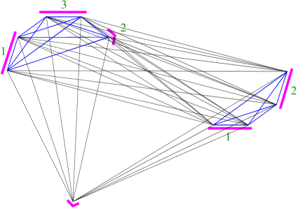
Figure 13. Intermediate representation schematic with $N=10$.

(0.D.3) For $N\in{\mathbb{N}}$, with the above notations, we have:

$${\mathfrak{S}}_{N}=\{(p,q,\rho,s)\;|\;p<q\in{\mathsf{P}}(N);\;\rho\in Perm_{p}(q);\;s\in{\mathsf{P}}_{2}(q/p)\}$$

One further schematic (neglecting only $s$) for elements of ${\mathfrak{S}}_{N}$ is as in Fig.13. In the schematic the well-separation of vertices again indicates $p$, thus   $p=\{\{\{1,2,3,4,5\},\{6,7,8,9\},\{\makebox[7.60002pt]{\hbox to0.0pt{\vrule width=7.60002pt,height=0.25832pt,depth=0.25832pt\hss}\hbox to0.0pt{\vrule width=7.60002pt,height=6.96246pt,depth=-6.44583pt\hss}\kern 0.5ptX\kern 0.5pt}\}\}$. The coloured bars indicate $q$, thus   $q=\{\{1,2\},\{3,4\},\{5\},\{6,7\},\{8,9\},\{\makebox[7.60002pt]{\hbox to0.0pt{\vrule width=7.60002pt,height=0.25832pt,depth=0.25832pt\hss}\hbox to0.0pt{\vrule width=7.60002pt,height=6.96246pt,depth=-6.44583pt\hss}\kern 0.5ptX\kern 0.5pt}\}\}$. And from the numbering   $Perm_{p}(q/p)=\{(\{1,2\},\{5\},\{3,4\}),(\{8,9\},\{6,7\}),(\{\makebox[7.60002pt]{\hbox to0.0pt{\vrule width=7.60002pt,height=0.25832pt,depth=0.25832pt\hss}\hbox to0.0pt{\vrule width=7.60002pt,height=6.96246pt,depth=-6.44583pt\hss}\kern 0.5ptX\kern 0.5pt}\})\}$. Up to $s$ data we thus have the same $\lambda\in{\mathfrak{S}}_{10}$ as in Fig.12,

References

- [AG18] Nicolás Andruskiewitsch and João Matheus Jury Giraldi. Nichols algebras that are quantum planes. Linear Multilinear Algebra, 66(5):961–991, 2018.
- [Art25] E. Artin. Theorie der Zöpfe. Abh. Math. Sem. Univ. Hamburg, 4(1):47 –72, 1925.
- [Bax82] R J Baxter. Exactly Solved Models in Statistical Mechanics. Academic Press, New York, 1982.
- [BB17] V M Bondarenko and M Yu Bortosh. Indecomposable and isomorphic objects in the category of monomial matrices over a local ring. Ukrainian Mathematical Journal, 69:1034–1050, 2017.
- [Bir75] J S Birman. Braids, Links and Mapping Class Groups, volume 82. Annals of Mathematics Studies, Princeton University Press, Princeton NJ, 1975.
- [BS07] John C. Baez and Urs Schreiber. Higher gauge theory. In Categories in algebra, geometry and mathematical physics. Conference and workshop in honor of Ross Street’s 60th birthday, Sydney and Canberra, Australia, July 11–16/July 18–21, 2005, pages 7–30. Providence, RI: American Mathematical Society (AMS), 2007.
- [DMR20] C Damiani, P Martin, and E Rowell. Generalisations of Hecke algebras from loop braid groups. arxiv, 2020.
- [Dri85] V. G. Drinfeld. Hopf algebras and the quantum Yang-Baxter equation. Dokl. Akad. Nauk SSSR, 283(5):1060–1064, 1985.
- [ESS99] Pavel Etingof, Travis Schedler, and Alexandre Soloviev. Set-theoretical solutions to the quantum Yang-Baxter equation. Duke Math. J., 100(2):169–209, 1999.
- [FS09] Philippe Flajolet and Robert Sedgewick. Analytic combinatorics. Cambridge University Press, Cambridge, 2009.
- [GJ89] David M. Goldschmidt and V. F. R. Jones. Metaplectic link invariants. Geom. Dedicata, 31(2):165–191, 1989.
- [Hie92] Jarmo Hietarinta. All solutions to the constant quantum Yang-Baxter equation in two dimensions. Phys. Lett. A, 165(3):245–251, 1992.
- [HMNR23] J. Hietarinta, P. Martin, F. Nijhoff, and E.C. Rowell. Additive charge-conserving braid representations. in preparation, 2023.
- [Jim86] M Jimbo. A -analogue of , Hecke algebra and the Yang–Baxter equation. Lett Math Phys, 11:247–252, 1986.
- [Jon85] Vaughan F. R. Jones. A polynomial invariant for knots via von Neumann algebras. Bull. Amer. Math. Soc. (N.S.), 12(1):103–111, 1985.
- [JS93] A Joyal and R Street. Braided tensor categories. Adv Math, 102:20–78, 1993. (Macquarie MR850067/860081).
- [KV94] M. M. Kapranov and V. A. Voevodsky. -categories and Zamolodchikov tetrahedra equations. In Algebraic groups and their generalizations: quantum and infinite-dimensional methods (University Park, PA, 1991), volume 56 of Proc. Sympos. Pure Math., pages 177–259. Amer. Math. Soc., Providence, RI, 1994.
- [Lan65] S Mac Lane. Categorical algebra. BAMS, 71:40–106, 1965.
- [Lan78] S Mac Lane. Categories for the working mathematician. GTM 5. Springer, 2nd edition, 1978.
- [LM77] Jon M Leinaas and Jan Myrheim. On the theory of identical particles. Il Nuovo Cimento B (1971-1996), 37(1):1–23, 1977.
- [Mar91] P P Martin. Potts Models and related problems in statistical mechanics. World Scientific, Singapore, 1991.
- [Mar92] P P Martin. On Schur-Weyl duality, Hecke algebras and quantum . Int J Mod Phys A, 7 suppl.1B:645–674, 1992.
- [Mar08] P P Martin. On diagram categories, representation theory and statistical mechanics. AMS Contemp Math, 456:99–136, 2008.
- [MM14] Volodymyr Mazorchuk and Vanessa Miemietz. Additive versus abelian 2-representations of fiat 2-categories. Mosc. Math. J., 14(3):595–615, 642, 2014.
- [MM16] Volodymyr Mazorchuk and Vanessa Miemietz. Transitive 2-representations of finitary 2-categories. Trans. Amer. Math. Soc., 368(11):7623–7644, 2016.
- [MP11] João Faria Martins and Roger Picken. Surface holonomy for non-abelian 2-bundles via double groupoids. Adv. Math., 226(4):3309–3366, 2011.
- [MRT23] Paul Martin, Eric C. Rowell, and Fiona Torzewska. Classification of charge-conserving loop braid representations. https://doi.org/10.48550/arxiv.2301.13831, 2023.
- [Mur38] F D Murnaghan. The Theory of Group Representations. Dover, 1938.
- [MW98] P P Martin and D Woodcock. On quantum spin–chain spectra and the structure of Hecke algebras and –groups at roots of unity. J Phys A, 31:10131–10154, 1998.
- [Par70] B Pareigis. Categories and Functors. Springer, 1970.
- [Pfe03] Hendryk Pfeiffer. Higher gauge theory and a non-abelian generalization of 2-form electrodynamics. Annals of Physics, 308(2):447–477, 2003.
- [RW12] Eric C. Rowell and Zhenghan Wang. Localization of unitary braid group representations. Comm. Math. Phys., 311(3):595–615, 2012.
- [RW18] Dmitriy Rumynin and Alex Wendland. 2-groups, 2-characters, and Burnside rings. Adv. Math., 338:196–236, 2018.
- [Slo21] N J A Sloane. The on-line encyclopedia of integer sequences, 2021. published electronically at http://oeis.org.
- [SP95] N. J. A. Sloane and S. Plouffe. The Encyclopedia of Integer Sequences. San Diego, CA, Academic Press, 1995. pp. 20-21.
- [Tur88] V. G. Turaev. The Yang-Baxter equation and invariants of links. Invent. Math., 92(3):527–553, 1988.
- [Yan67] C N Yang. Some exact results for the many-body problem in one dimension with repulsive delta-function interaction. Rev. Lett., 19:1312, 1967.