Extreme $\ell$-boson stars

Abstract

A new class of complex scalar field objects, which generalize the well known boson stars, was recently found as solutions to the Einstein-Klein-Gordon system. The generalization consists in incorporating some of the effects of angular momentum, while still maintaining the spacetime’s spherical symmetry. These new solutions depend on an (integer) angular parameter $\ell$, and hence were named $\ell$-boson stars. Like the standard $\ell=0$ boson stars these configurations admit a stable branch in the solution space; however, contrary to them they have a morphology that presents a shell-like structure with a “hole” in the internal region. In this article we perform a thorough exploration of the parameter space, concentrating particularly on the extreme cases with large values of $\ell$. We show that the shells grow in size with the angular parameter, doing so linearly for large values, with the size growing faster than the thickness. Their mass also increases with $\ell$, but in such a way that their compactness, while also growing monotonically, converges to a finite value corresponding to about one half of the Buchdahl limit for stable configurations. Furthermore, we show that $\ell$-boson stars can be highly anisotropic, with the radial pressure diminishing relative to the tangential pressure for large $\ell$, reducing asymptotically to zero, and with the maximum density also approaching zero. We show that these properties can be understood by analyzing the asymptotic limit $\ell\rightarrow\infty$ of the field equations and their solutions. We also analyze the existence and characteristics of both timelike and null circular orbits, especially for very compact solutions.

I Introduction

The possibility that dark matter can be described by a scalar field has recently found an increasing interest, either through the study of models with a particle physics motivation Preskill et al. (1983); Abbott and Sikivie (1983); Dine and Fischler (1983); Zyla et al. (2020), or through the description of lighter fields with the potential to alleviate some possible tensions in the standard cosmological scenario on small scales Marsh (2016); Hui et al. (2017); Niemeyer (2019); Hu et al. (2000); Matos et al. (2000); Matos and Ureña López (2001); Matos et al. (2008) (see e.g. Genina et al. (2018); Kendall and Easther (2020); Kim et al. (2018); Nadler et al. (2021) for updated discussions on the classical cold dark matter problems). Gravitationally bound bosonic structures appearing as the consequence of these fields may be relevant in astrophysics, as they could develop dark matter halos and/or very compact objects, depending on the particular choice of the parameters of the model. In the high compactness regime, bosonic structures can approach the Buchdahl limit Buchdahl (1959) and form objects similar in size and mass to neutron stars or even black holes. Like other compact objects Cardoso and Pani (2019), boson stars Jetzer (1992); Liddle and Madsen (1992); Mielke and Schunck (1997); Liebling and Palenzuela (2017); Visinelli (2021) may form bound binary systems emitting gravitational waves of distinctive features. The dynamics of these systems has been studied for instance in references Palenzuela et al. (2017); Bezares et al. (2017); Bezares and Palenzuela (2018) (see also Bustillo et al. (2021) where the waveforms calculated from the head-on collision between two Proca stars is confronted with gravitational wave observations). On the other hand, in the low compactness regime, gravitationally bound structures can be used to describe dark matter halos Sin (1994); Lee and Koh (1996); Arbey et al. (2003), although some controversies have arisen regarding the non-compatibility on the required values of the field mass when combining different data sets. For example, the characteristic masses needed to describe the internal kinematics of the Milky Way dwarf spheroidal satellites are in tension when faced with cosmology Gonzalez-Morales et al. ([arXiv:1609.05856], 2016) (see also Hayashi et al. (2021)), and even at local scales the mass density profiles of dwarf spheroidal and ultra-faint dwarf galaxies suggest different values for the field mass Hayashi et al. (2021); Safarzadeh and Spergel (2019). Furthermore, for larger galaxies the dark matter halos could be even more cuspy than the standard cold dark matter Navarro-Frenk-White profiles Robles et al. (2019). These problems emerge when fitting the observations to the dark matter halo profile predicted by a standard boson star, in some cases enlarged with an external Navarro-Frenk-White profile as suggested by numerical cosmological simulations Schive et al. (2014a, b); Schwabe et al. (2016); Veltmaat and Niemeyer (2016). However, in recent years, it has been argued that more general stable, self-gravitating scalar field objects could exist in nature, and this may affect the previous conclusions.

An interesting example of such configurations are the $\ell$-boson stars we have presented in previous work Alcubierre et al. (2018). Based on similar ideas used previously in the context of gravitational collapse Olabarrieta et al. (2007), $\ell$-boson stars incorporate some effects of the angular momentum into the scalar fields while maintaining the spherical symmetry of the spacetime, which results in a relatively simple model for their description. In the particular case where $\ell=0$ the standard boson stars by Kaup Kaup (1968) and Ruffini and Bonazzola Ruffini and Bonazzola (1969) are recovered. However, in general, in addition to the parameters that characterize the standard $\ell=0$ solutions, there is an “angular momentum number” $\ell$ that provides a model with a richer structure that could potentially be relevant for the description of dark matter halos and compact objects. In particular, and as we further explore in this article, boson stars with $\ell>0$ can be more compact than standard ones. It turns out that the maximum mass of these objects increases greatly with $\ell$, giving masses that are orders of magnitude larger than for the $\ell=0$ case. Even if these configurations are also larger in size than the standard ones, the growth in mass is faster than the growth in size in such a way that the compactness increases.

The stability of $\ell$-boson stars under spherical perturbations has first been studied in Alcubierre et al. (2019) by performing numerical evolutions of the Einstein-Klein-Gordon equations in spherical symmetry, and later also in Alcubierre et al. (2021) based on a more formal study of the linearized system. These analyses have revealed that $\ell$-boson stars show stability characteristics that are qualitatively similar to those of the $\ell=0$ case, where for each value of $\ell$ there exist a stable and an unstable branch with the transition point given by the solution of maximum total mass. For other studies addressing the stability of $\ell$-boson stars which are based on full nonlinear numerical evolutions without symmetries see Jaramillo et al. (2020); Sanchis-Gual et al. (2021) (see also Guzmán and Ureña López (2020) for a study of the Newtonian regime in axial symmetry). In particular, in Sanchis-Gual et al. (2021) it was shown that $\ell$-boson stars assume a privileged role among other stationary solutions of the multi-field, multi-frequency scalar field scenario as far as their stability is concerned.

In the present work we perform an exhaustive exploration of the $\ell$-boson stars’ parameter space, focusing in particular on solutions with very large values of $\ell$, including the $\ell\rightarrow\infty$ limit. Our analysis covers the stars’ morphology, anisotropy and compactness, the characteristics of the circular orbits (including the null ones, also known as light rings), as well as the scaling properties of the fields and relevant physical quantities with respect to $\ell$. We start in section II with a brief review of $\ell$-boson stars, presenting the main equations and properties, including the definitions of density, pressure, anisotropy and compactness, and present the equations for geodesic motion, particularly those describing circular causal geodesics. Next, in section III, we present our solutions, analyzing in each case the role played by the angular momentum parameter $\ell$ on various of their properties, and paying particular attention to the large $\ell$ regime. We accomplish this by numerically obtaining and analyzing hundreds of solutions. The observed scaling properties of the fields for large $\ell$ motivate the in-depth study of section IV, where we obtain effective equations which describe the asymptotic behavior of the fields in the limit $\ell\rightarrow\infty$. Conclusions and an overview of our results are given in section V. Technical details and tables summarizing our notation and numerical data are included in appendices A–C.

Throughout this work we use the signature convention $(-,+,+,+)$ for the spacetime metric and Planck units such that $G=c=\hbar=1$. We present our results in a form that is independent of the scalar field mass $\mu$. The rescaling rules in $\mu$ are summarized in table 2 of appendix A.

II $\ell$-boson stars

In this section we summarize the relevant equations that describe $\ell$-boson stars, as well as some of their most significant properties. Additional information can be found in our previous works Alcubierre et al. (2018, 2019, 2021); see also the review articles Jetzer (1992); Liddle and Madsen (1992); Mielke and Schunck (1997); Liebling and Palenzuela (2017); Visinelli (2021) for the standard $\ell=0$ boson stars. $\ell$-Boson stars are self-gravitating objects that consist of an odd number $N=2\ell+1$ of complex scalar fields $\Phi_{\ell m}$, $m=-\ell,\ldots,\ell$ of equal mass $\mu$ and the same radial profile. The dynamics of these fields is described by the following Lagrangian

$$\mathcal{L}=\frac{R}{16\pi}-\frac{1}{2}\sum_{m=-\ell}^{\ell}\left(\nabla_{\mu}\Phi_{\ell m}\nabla^{\mu}\Phi^{*}_{\ell m}+\mu^{2}{|\Phi_{\ell m}|}^{2}\right),$$ (1)

where $R$ is the Ricci scalar and the scalar fields have the form:

$$\Phi_{\ell m}(t,r,\vartheta,\varphi)=e^{i\omega t}\psi_{\ell}(r)Y^{\ell m}(\vartheta,\varphi),$$ (2)

with $\omega$ a real frequency and $\psi_{\ell}$ a real-valued radial function which is independent of $m$. As usual, $Y^{\ell m}$ denote the standard spherical harmonics with angular momentum numbers $\ell$ and $m$. By applying the addition theorem for spherical harmonics one can see that in the absence of self-interactions, the total stress energy-momentum tensor

$$T_{\mu\nu}=\frac{1}{2}\sum_{m=-\ell}^{\ell}\left[\nabla_{\mu}\Phi_{\ell m}^{*}\nabla_{\nu}\Phi_{\ell m}+\nabla_{\mu}\Phi_{\ell m}\nabla_{\nu}\Phi_{\ell m}^{*}-g_{\mu\nu}\left(\nabla_{\alpha}\Phi_{\ell m}^{*}\nabla^{\alpha}\Phi_{\ell m}+\mu^{2}\Phi_{\ell m}^{*}\Phi_{\ell m}\right)\right]$$ (3)

is spherically symmetric, even if $\ell>0$ ($N>1$) and the individual fields have angular momentum.

The spacetime metric is parameterized according to

$$ds^{2}=-\alpha^{2}(r)dt^{2}+\gamma^{2}(r)dr^{2}+r^{2}d\Omega^{2},\qquad\gamma^{2}(r):=\frac{1}{1-\frac{2M(r)}{r}},$$ (4)

where $\alpha$ and $M$ denote the lapse and the Misner-Sharp mass functions, respectively, $r$ is the areal radius and $d\Omega^{2}$ is the standard metric on the unit two-sphere. The field equations are obtained from the Einstein-Klein-Gordon system and take the form Alcubierre et al. (2018):

$$M^{\prime}=\frac{\kappa_{\ell}r^{2}}{2}\left[\frac{\psi_{\ell}^{\prime 2}}{\gamma^{2}}+\left(\mu^{2}+\frac{\omega^{2}}{\alpha^{2}}+\frac{\ell(\ell+1)}{r^{2}}\right)\psi_{\ell}^{2}\right]=4\pi r^{2}\rho,$$ (5a)

$$\frac{(\alpha\gamma)^{\prime}}{\alpha\gamma^{3}}=\kappa_{\ell}r\left[\frac{\psi_{\ell}^{\prime 2}}{\gamma^{2}}+\frac{\omega^{2}}{\alpha^{2}}\psi_{\ell}^{2}\right]=4\pi r(\rho+p_{r}),$$ (5b)

$$\frac{1}{r^{2}\alpha\gamma}\left(\frac{r^{2}\alpha}{\gamma}\psi_{\ell}^{\prime}\right)^{\prime}=\left(\mu^{2}-\frac{\omega^{2}}{\alpha^{2}}+\frac{\ell(\ell+1)}{r^{2}}\right)\psi_{\ell},$$ (5c)

whith $\kappa_{\ell}:=2\ell+1$, and where we have introduced the energy density, radial pressure and tangential pressure defined as:

$$\rho:=-{T^{t}}_{t}= \frac{\kappa_{\ell}}{8\pi}\left[\;\;\;\frac{{\psi_{\ell}^{\prime}}^{2}}{\gamma^{2}}+\frac{\omega^{2}}{\alpha^{2}}\psi_{\ell}^{2}+\left(\mu^{2}+\frac{\ell(\ell+1)}{r^{2}}\right)\psi_{\ell}^{2}\right],$$ (6a)

$$p_{r}:={T^{r}}_{r}= \frac{\kappa_{\ell}}{8\pi}\left[\;\;\;\frac{{\psi_{\ell}^{\prime}}^{2}}{\gamma^{2}}+\frac{\omega^{2}}{\alpha^{2}}\psi_{\ell}^{2}-\left(\mu^{2}+\frac{\ell(\ell+1)}{r^{2}}\right)\psi_{\ell}^{2}\right],$$ (6b)

$$p_{T}:={T^{\theta}}_{\theta}={T^{\varphi}}_{\varphi}= \frac{\kappa_{\ell}}{8\pi}\left[-\frac{{\psi_{\ell}^{\prime}}^{2}}{\gamma^{2}}+\frac{\omega^{2}}{\alpha^{2}}\psi_{\ell}^{2}-\mu^{2}\psi_{\ell}^{2}\right].$$ (6c)

We denote by $M_{T}$ the total mass of the object, given by the limit $r\to\infty$ of the function $M(r)=4\pi\int_{0}^{r}\,\tilde{r}^{2}\,\rho(\tilde{r})\,d\tilde{r}$. In the case of our numerical solutions, we approximate $M_{T}$ by evaluating $M(r)$ a the outer boundary of the numerical domain (after ensuring that the mass variation is negligible near that boundary).

Each $\ell$-boson star solution is uniquely determined by a given set of the parameters $\ell$, $\mu$, $u_{0}$, and a discrete set of values $\omega$, with $u_{0}$ given by $\psi_{\ell}/r^{\ell}$ evaluated at $r=0$. Given $\ell$ and $\mu$, $u_{0}$ is a free parameter (which reduces to the central scalar field amplitude $\psi_{c}=\psi(r=0)$ for $\ell=0$), and the $\omega$’s are the frequency eigenvalues obtained by demanding that the field vanishes at infinity and that the solution remains regular at $r=0$. In this work we only consider the ground state for which $\psi_{\ell}$ has no nodes in the open interval $r\in(0,\infty)$, hence fixing $\omega$ for each $\ell$ and $u_{0}$. Finally, solutions with different $\mu$ are related to each other by a simple rescaling (see table 2 in appendix A). Consequently, for each $\ell$ it is sufficient to study a one-parameter family of solutions, usually parameterized by $u_{0}$ or (equivalently) by $\alpha_{0}:=\alpha(r=0)$.

Since boson stars do not have a well defined boundary, one usually describes their size by the $R_{99}$ radius, defined as the (areal) radius of the sphere containing 99% of the total mass $M_{T}$. In addition, we use two different measures for the star’s compactness:

$$C_{99}:=\frac{M_{T}}{R_{99}},$$ (7a)

and

$$C_{m}:=\max\limits_{r>0}\left\{\frac{M(r)}{r}\right\}=:\frac{M_{m}}{R_{m}},$$ (7b)

where we also defined $R_{m}$ as the point $r$ of maximum $M(r)/r$, and $M_{m}$ as $M(r=R_{m})$. To help better understand the meaning of these definitions we highlight their differences in the top panel of figure 1, where some density profiles are shown, together with vertical lines indicating the radii $R_{99}$ and $R_{m}$ for each star.

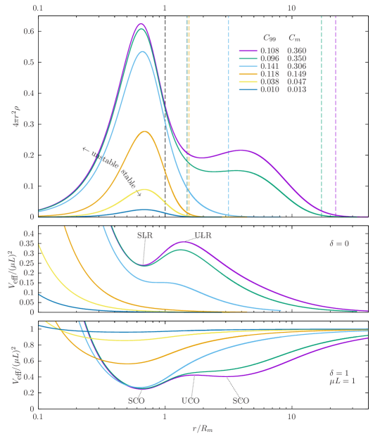
Figure 1: Top panel: For various configurations with $\ell=1$, we show the rescaled density profile with respect to the rescaled radial coordinate $r\rightarrow r/R_{m}$. This rescaling provides an easier way to compare the different curves between themselves, while also allowing to easily locate $R_{m}$, given by $r/R_{m}=1$ (black vertical line), as well as $R_{99}$ (vertical lines with the same color as the corresponding solution). Middle panel: Effective potentials for circular null geodesics ($\delta=0$) for the same solutions as in the top panel, displaying cases without light rings, with a pair of (stable and unstable) light rings, and the transition solution for which the (degenerate) light rings first appear. Bottom panel: Effective potentials for circular timelike geodesics ($\delta=1$) with $\mu L=1$ for the same solutions as in the other panels. The local extrema correspond to stable (minimum) and unstable (maximum) circular orbits.

As one can appreciate from this figure, some solutions (see for instance the purple and green lines) can be interpreted as having two parts: A very compact “core”, located mostly to the left of $r/R_{m}=1$, plus a less dense “halo” to the right of that point. Note that the halo is much wider than the central region (a fact that might be unnoticed at a first glance since the horizontal axis is in logarithmic scale). We clearly see that the definition $C_{99}$ is a proper indicator of the whole object’s compactness, while the definition $C_{m}$ is more representative of the central region’s compactness. However, as we will see later, the sets of definitions $\left[R_{99},M_{T},C_{99}\right]$ and $\left[R_{m},M_{m},C_{m}\right]$ tend to coincide for larger $\ell$’s. Although we have found the core-and-halo structure only for configurations lying on the unstable branches, the mentioned differences between these two sets are seen for stable as well as unstable solutions.

The stress tensor of a perfect fluid is isotropic, and pressure is the same in all directions of a fluid star. Even if common for some materials, isotropy is not a natural consequence of the underlying spacetime symmetries, and there exist static and spherical configurations that exhibit fractional anisotropy, defined as the relative difference between the radial and tangential components of the pressure:

$$fa=\frac{p_{r}-p_{T}}{p_{r}}.$$ (8)

From the right-hand sides of equations (6b) and (6c) one can see that $\ell$-boson stars (including the standard $\ell=0$ boson stars) are anisotropic. Furthermore, one might suspect that solutions with higher anisotropy will exist for the cases with non-vanishing angular momentum number, due to the presence of the centrifugal term $\ell(\ell+1)/r^{2}$ in $p_{r}$. We will corroborate this assertion in the next sections. This is not just a curious fact, since configurations with larger fractional anisotropy have been identified to be stable up to higher values of the central density Gleiser (1988), hence leading to more compact objects Dev and Gleiser (2002). This enhancement in the allowed compactness within the stable branch is an interesting property that is also satisfied for $\ell$-boson stars, as we discuss later.

It will also be helpful to identify some general properties of the motion of test particles propagating in the spacetime associated with the $\ell$-boson stars, and in particular to determine whether the solutions admit innermost stable circular orbits (ISCOs) and/or light rings Cardoso and Pani (2019) and, if so, to find their location. Given the spacetime symmetries we can obtain the geodesics with the help of conserved quantities using the expression Wald (1984)

$$\left(\frac{dr}{d\lambda}\right)^{2}=\frac{E^{2}}{\alpha^{2}\gamma^{2}}-\frac{1}{\gamma^{2}}\left(\delta+\frac{L^{2}}{r^{2}}\right),$$ (9)

where $E$ and $L$ are constants of motion (associated with the particle’s energy and total angular momentum), and $\delta=0$ for null geodesics, while $\delta=1$ for timelike geodesics. It is convenient to introduce the effective potential

$$V_{\rm eff}(r):=\alpha^{2}\left(\delta+\frac{L^{2}}{r^{2}}\right),$$ (10)

leading to an equation of motion that resembles a point particle moving in a one-dimensional potential. Then, orbiting particles are restricted to the regions where $V_{\rm eff}(r)<E^{2}$. Circular orbits can be obtained when $E^{2}$ equals a local extremum of $V_{\rm eff}$, and those orbits are stable (unstable) if said extremum is a minimum (maximum).

In the null case, the condition for circular orbits is

$$\alpha-r\,\alpha^{\prime}=0,$$ (11)

where the sign of the second derivative of the lapse function evaluated at the light ring radius determines the stability of the orbit: it is stable if $\alpha^{\prime\prime}$ is negative and unstable otherwise Barranco et al. (2021). In the timelike case the energy and total angular momentum per unit rest mass of a particle in circular motion at radius $r$ must satisfy

$$E=\sqrt{\frac{\alpha^{3}}{\alpha-r\alpha^{\prime}}},\quad L=\sqrt{\frac{r^{3}\alpha^{\prime}}{\alpha-r\alpha^{\prime}}}.$$ (12)

These orbits are stable wherever $L(r)$ grows with $r$, whereas they are unstable otherwise Barranco et al. (2021). For regular configurations light rings can appear only in pairs, one of them being stable and the other unstable. Note, however, that not all stars admit light rings. On the other hand, there always exist stable circular orbits of massive particles. In particular, the existence of stable orbits is guaranteed both at large distances and close enough to the center. However, regions of instability may exist too, being delimited by innermost stable circular orbits (ISCOs) and outermost stable circular orbits (OSCOs). In a similar way, the light ring pairs delimit a region where $\alpha-r\,\alpha^{\prime}$ is negative and circular orbits are not allowed at all. We will now give more explicit details about these assertions.

The central panel of figure 1 illustrates distinct cases regarding the existence of light rings, as determined by equation (10), all with $\ell=1$: (i) Potentials without local extrema (besides at $r=0$). These solutions cannot have light rings. (ii) Potentials with a local minimum at some $r=r_{\rm in}$ and with a local maximum at some other $r=r_{\rm out}$, such that $r_{\rm in}<r_{\rm out}$. These solutions have a pair of light rings, a stable one at $r_{\rm in}$ and an unstable one at $r_{\rm out}$. (iii) The transition case, in which the potential have an inflection point, giving rise to degenerate light ring solutions with $r_{\rm in}=r_{\rm out}$. Note that cases (ii) and (iii) only occur for unstable spacetimes Alcubierre et al. (2019, 2021). In a similar way, in the bottom panel of this figure we illustrate different cases regarding the existence of unstable circular orbits of massive particles with $\mu L=1$.

Finally, we give an expression for the test particle’s speed moving on a circular orbit (more precisely, the magnitude of its three-velocity as measure by a static observer located at the corresponding radius):

$$v(r):=r\frac{d\phi}{dt}=\sqrt{\frac{r\alpha^{\prime}(r)}{\alpha(r)}},$$ (13)

which will be used in the next section to show some rotation curves.

III Extreme $\ell$-boson stars

In this section we present and analyze our results. For all integer $\ell$ from $0$ to $15$, and for $\ell=20$, $25$, $50$, $75$, $100$, $200$, $400$ and $1600$, we constructed solutions, tens of them in some cases, that correspond to different values of the central parameter $u_{0}$. The parameters and main properties of some of the most relevant solutions that we have obtained are displayed in table 3 of appendix C, which also includes a reference to the figures in which they are used. In addition, in the next section we obtain general expressions that are applicable for the limiting case in which $\ell\rightarrow\infty$.

We present some of our solutions in figure 2, where we show the rescaled density profiles (defined as $\varrho=4\pi r^{2}\rho$ such that $M=\int\varrho dr$) associated with some of our configurations. Since one needs some criterion in order to compare solutions through different values of $\ell$, in this case we chose to display configurations that, for each $\ell$, have the maximum total mass, which are also the most compact stable solutions. This is a criterion we will adopt in most of this work. In the same figure we also show some solutions for given $\ell$ ($=25$) and varying compactness, the more compact ones being unstable. The solutions clearly exhibit a shell-like morphology, at least for $\ell>1$. For bigger $\ell$ the stars are larger both in size and in total mass. We will see that the compactness also increases with $\ell$. In contrast, if one considers stars with fixed $\ell$ and increasing size, the compactness decreases. We also note that, as is the case for the traditional $\ell=0$ boson stars, the most compact solutions belong to the unstable branch.

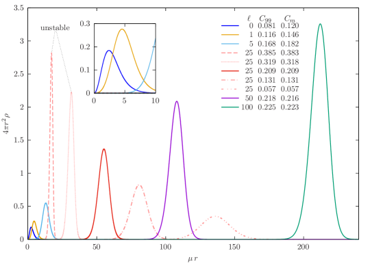
Figure 2: Rescaled density profiles, $4\pi r^{2}\rho(r)$, of solutions with maximum $M_{T}$ for various values of $\ell$ (solid lines), and of varying compactness for fixed $\ell=25$, both in the stable and unstable region (red lines). The inner panel shows a zoom into the small $r$ region for a better reference of the cases with $\ell=0$ and $1$.

Figure 3 shows the dependence of the total mass on the frequency and on the $R_{99}$ radius for $\ell=0$, $1$, $5$, $25$, $50$ and $100$. For each $\ell$ we indicate the maximum of $M_{T}$ (squares), which we denote $M_{\rm max}$, and the first appearance of a light rings pair (circles) and of an ISCO-OSCO pair (triangles). We have seen in previous works Alcubierre et al. (2019, 2021) that the state of maximum mass marks the transition from the stable solutions (to the right in these figures) to the unstable ones (to the left) for $\ell$ in the interval from 0 to 5. We also corroborated in the present work that this fact is still true for larger values of $\ell$.

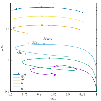
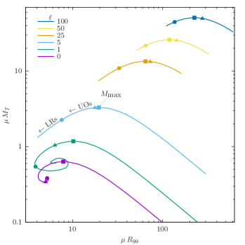
Figure 3: $M_{T}$ vs. $\omega$ and vs. $R_{99}$ for $\ell=0$, $1$, $5$, $25$, $50$ and $100$. Each point on these curves corresponds to a different solution, including for instance those shown in figure 2. The squares denote the maximum of the total mass, which separates the stable and unstable regions. The circles denote the first appearance of light rings, while the triangles denote the first appearance of an ISCO-OSCO pair and, hence, the existence of unstable orbits (UOs).

In the following subsections we analyze various properties of these solutions, including their compactness, anisotropy and causal circular orbits.

III.1 Compactness

In this section we explore the compactness of our solutions using the definitions of equations (7). As can be seen from figure 3, larger values of $\ell$ lead to solutions with higher total mass $M_{T}$. On the other hand, considering for instance the solutions of maximum mass, the radius also increases with $\ell$, as can be inferred from that same figure and figure 2. However, the increase in mass tends to “win” over the increase in radius in such a way that their ratio, the compactness, increases with $\ell$. Note that said solutions are the most compact stable ones for each $\ell$.

After inspection of our solutions we note that the two mass definitions $M_{T}$ and $M_{m}$ from equations (7), as well as their associated radii $R_{99}$ and $R_{m}$, seem to both show a linear relation with $\ell$, at least at large $\ell$ ($\ell\gtrsim 10$). This can be seen in the first two panels of figure 4. Once again, in order to compare configuration with different $\ell$’s between each other, we have chosen those solutions with maximum total mass $M_{\textrm{max}}$ for each $\ell$.

The apparent linear dependence in $\ell$ suggests that simple expressions can be obtained by performing linear fits. We show the results of said fits in the figure (continuous lines), together with the fit coefficients ($a$ to $d$) and their respective errors. Keeping only two significant figures and omitting the errors we can write:

$$\mu M_{T} \approx 0.50\,\ell+0.82,$$ (14a)

$$\mu M_{m} \approx 0.50\,\ell+0.55,$$ (14b)

$$\mu R_{99} \approx 2.2\,\ell+8.7,$$ (14c)

$$\mu R_{m} \approx 2.2\,\ell+6.7.$$ (14d)

From here, expressions for our two definitions of compactness can be found by taking the quotient of each $M$ vs. $R$ pair. Said quotients, i.e. $C_{99}$ and $C_{m}$, are shown in the last panel of figure 4. The point values shown in that panel are obtained by taking individually the quotient of the corresponding data pairs that appear in the first panels, while the continuous line represent the quotient of the linear fit’s expressions.

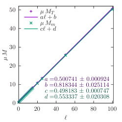
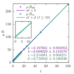
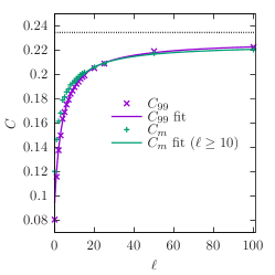
Figure 4: We show the dependence on $\ell$ of the stars’ mass, radius and compactness. All quantities shown here correspond to the solution of maximum $M_{T}$ for each value of $\ell$. Left panel: $M_{T}$ and $M_{m}$, together with the corresponding linear fits. Center panel: $R_{99}$ and $R_{m}$, together with their linear fit. In the case of $R_{m}$ we do the linear fit only to the points with $\ell\geq 10$, which is the region where we actually see a linear dependence. Right panel: Compactness $C_{m}$ and $C_{99}$, and, in each case, the compactness calculated from the fits of the previous panels. We also indicate the asymptotic value as a dotted line (see section IV).

The almost linear relations shown in the first two panels of figure 4 suggest that solutions might have simple rescaling properties with $\ell$, at least at large enough $\ell$. A more detailed analysis of such scaling properties will be given in section IV, where we will see that an asymptotic value can be obtained for the compactness at large $\ell$. That value is indicated in the right panel of figure 4 as a dotted line. Note that initially the compactness increases rapidly with $\ell$, and continues to rise monotonically, remaining close to and below the asymptotic value derived in section IV.

III.2 Anisotropy

We move now to the description of the stars’ anisotropy. In figure 5 we show the pressure profiles for $\ell=0$, $1$, $5$ and $25$, in all cases for the solution of maximum mass $M_{\rm max}$. Notice how different the profiles are for $\ell=0$, $\ell=1$, and $\ell>1$. The typical $\ell=0$ “solid-sphere” star has $p_{r}>p_{T}$, while for larger $\ell$’s the “shell-like” stars have mostly $p_{r}<p_{T}$, with this difference becoming more pronounced the higher the value of $\ell$. This behavior seems intuitively natural given the stars’ morphology. As $\ell$ increases, the ”shells” become larger, as well as thinner relative to their radius, in such a way that the tangential pressure has to become larger relative to the radial one in order to support the configuration.

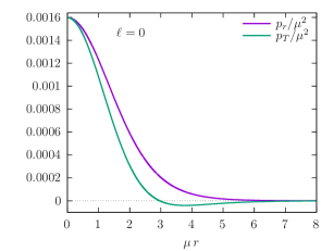
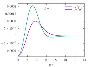
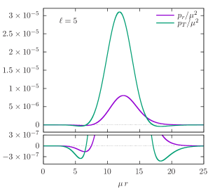
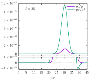
Figure 5: Radial and tangential pressures vs. radial coordinate for the solutions of maximum $M_{T}$ in the cases of $\ell=0$, 1, 5 and 25. We see that the tangential pressure becomes larger and larger relative to the radial pressure when $\ell$ increases.

In figure 6 we show parametric plots of [$p_{r}$,$p_{T}$] vs. $r$, in which the larger the deviation from the identity $p_{r}=p_{T}$ (shown as a dotted line of unit slope), the larger the anisotropy. Additionally, we indicate the density as a color map, as well as the compactness in each case. The differences at the starting points of these curves, which correspond to the pressure values at the origin $r=0$, are consistent with the stars’ shape as seen in our previous work: while they are “empty” at the center when $\ell>1$, they have maximum density there when $\ell=0$, as is a well known property of standard boson stars. In the intermediate case, $\ell=1$, the density is greater than zero at the center, but it does not reach its maximum value at that point. It is also clear from these plots that the anisotropy, as well as the compactness, grow with $\ell$, the tangential pressure becoming larger and larger compared to the radial pressure. In section IV we will see that the limiting case $\ell\rightarrow\infty$ would display a vertical line in this type of plot. On the other hand, we see little differences in anisotropy when transitioning between stable and unstable solutions for any given value of $\ell$.

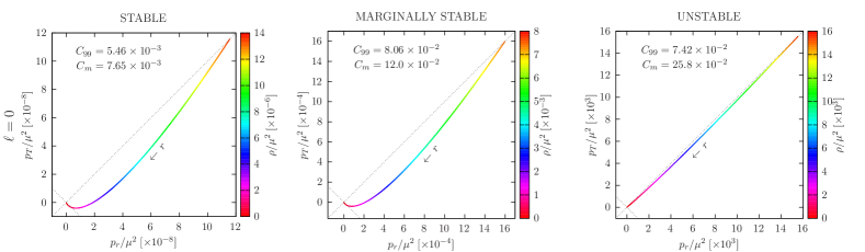
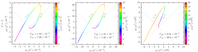
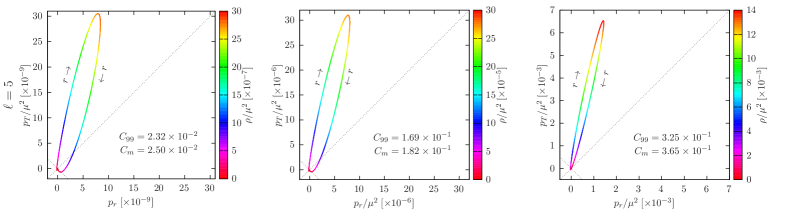
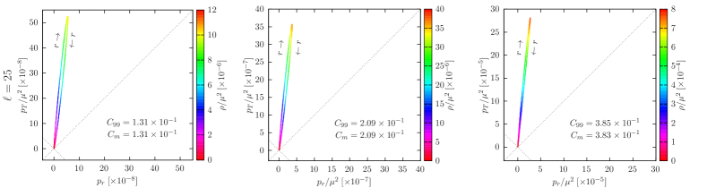
Figure 6: Parametric plots of $[p_{r},p_{T}](r)$. Each row corresponds to a value of $\ell$, while each column corresponds to a stability type. These figures are particularly well suited for analyzing the pressure anisotropies, measured by the deviation from the identity $p_{r}=p_{T}$. The value of the density $\rho$ along the curves is indicated with a color map. The direction of growing $r$ is also indicated. To help guide the eye, the curves $p_{r}=\pm p_{T}$ are shown as dotted lines, and the same scale was used in each pair of axes.

III.3 Geodesic motion

Given the large compactness that $\ell$-boson stars may achieve, one may wonder whether they admit light rings and/or ISCOs/OSCOs. In fact, it is known that even traditional $\ell=0$ boson stars can have light rings and ISCOs/OSCOs, although this is true only in the case of solutions located very deep into the unstable region. In the remainder of this section we will analyze the appearance of light rings and ISCOs/OSCOs, paying particular attention to their relation with compactness and stability of the underlying spacetime solutions.

In figure 3 we indicated with a circle the point corresponding to the first, or less compact, solutions containing a pair of light rings. In all the cases we studied, such solutions are always in the unstable region, although they get closer to the stable region as $\ell$ increases. It is unclear, however, whether light rings may be found in the stable region for large enough $\ell$, although one would expect that this is not the case given that the maximum compactness that a stable $\ell$-boson star is able to achieve, $C\approx 0.235$, is far from the expected one for the appearance of light rings, $C=1/3$. The results presented in Cunha et al. (2017) seem to indicate that light rings can only exist for unstable solutions. A recent work Guo et al. (2021) also presents results that support that hypothesis. Another matter of astrophysical interest is whether such unstable solutions have a relatively short or a rather long life-time. However, this question goes beyond the scope of the present article, so we leave it for future work.

Regarding the existence of ISCOs, we also indicated in figure 3 the first appearance of an ISCO-OSCO pair (triangles). We see that for large enough $\ell$ these pairs can also exist in the case of stable spacetime solutions. In fact, we have found that the smallest $\ell$ for which stable $\ell$-boson stars with ISCO-OSCO pairs exist is $\ell=9$.

We now go into more detail and analyze the different stability regions in figure 7, where we show plots of radius vs. compactness for $\ell=0$, 1, 5 and 25. Each vertical line in these plots corresponds to a solution, and we can see the transitions through different stability regions as $r$ varies along said line. The green regions are those where the timelike circular orbits are stable (SCOs). The red region is where the circular orbits are unstable (UCOs), and it is delimited by an ISCO at the top and by an OSCO at the bottom. Similarly, the dark gray region is that for which no circular orbitss exist, and it is delimited by a pair of light rings, indicated with a red line. Since $\ell$-boson stars are shell like for $\ell>1$, with density much smaller than its maximum value and falling quickly towards the center in the interior region –where the spacetime is very close to Minkowski– the circular orbits are almost non-existent there, having speed $v\ll 1$. To make this more apparent we shaded in a darker green the regions in which $v<10^{-5}$, noting that the rotation curves of these configurations have a maximum in the interval $0.4\lesssim v<1$ (see figure 8).

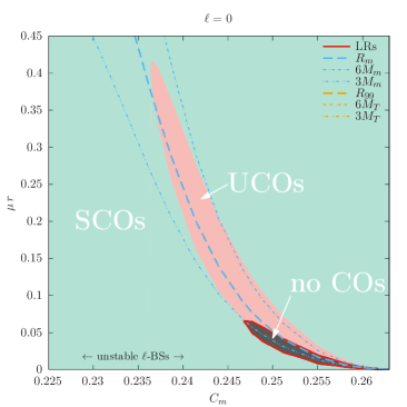
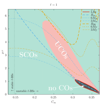
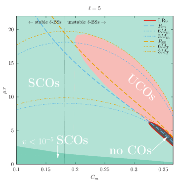
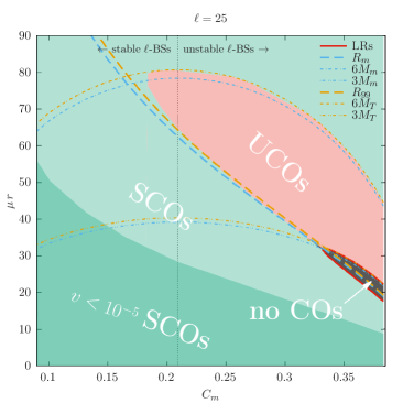
Figure 7: For solutions of high compactness we indicate the regions of existence and stability of causal circular orbits (COs). In these plots, each vertical line of constant $C_{m}$ corresponds to a different solution. The green regions indicate the radii with stable (timelike) circular orbits (SCOs), while the red region indicates those with unstable orbits (UCOs). On the other hand, no COs exist in the dark gray region, which is limited by a pair of light rings (LRs), red line. Finally, the dark green region indicates the “almost empty, almost flat” central region of the $\ell>1$ “shells”, where the circular orbits have speed $v<10^{-5}$. We also include as a guide $R_{99}$, $R_{m}$, and the corresponding locations of a Schwarzschild LR and ISCO.

Figure 7 also indicates the stars’ radii, $R_{99}$ and $R_{m}$, and also, as a guide, the limit of spacetime stability (vertical dotted line) and the locations of the Schwarzschild ISCO and light ring, given by $r=6M$ and $r=3M$, respectively, where for the value of $M$ we used both $M_{T}$ and $M_{m}$. We see that, as the compactness increases, the light rings first appear at or very close to $R_{m}$, and soon they move to each side of that location. For small $\ell$ the definition $R_{m}$ seems more meaningful than $R_{99}$ when comparing to the location of light rings. On the other hand, both definitions tend to coincide at large $\ell$.

Although all the solutions with light rings found in this work are unstable, we see that, for larger values of $\ell$, solutions with light rings exist closer and closer to the stable region. However, as mentioned earlier, it is unlikely that stable solutions with light rings exist, even for extremely large $\ell$.

Interestingly, the unstable circular orbit regions for large $\ell$ tend to be delimited almost exactly by the star’s radius (from below) and the Schwarzschild ISCO (from above). We can see again in the last panel of figure 7 ($\ell=25$) that regions of instability can exist even for stable $\ell$-boson star spacetimes. As already mentioned, this happens for solutions starting at $\ell=9$. This could constitute an observable feature that might help distinguish some $\ell$-boson stars from other dark compact objects.

In figure 8 we show the rotation curves for the solutions shown in figure 2, that is: solutions of maximum $M_{T}$ for $\ell=0$, 1, 5, 25, 50 and 100; and for $\ell=25$, also some solutions with varying compactness, both in the stable and unstable spacetime branch. The curves have been extended beyond the domain of numerical integration using the Schwarzschild expressions with mass $M_{T}$. We can see that this gives and excellent match. The points where the curves reach $v=1$ correspond to light rings, and no circular orbits exist in the region in between those points (red line and dark gray region of figure 7). We also indicate the regions where the circular orbits are unstable (thick gray line).

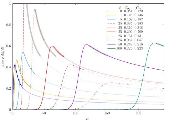
Figure 8: Rotation curves as defined by equation (13). The solid lines correspond to solutions with maximum $M_{T}$ for $\ell$ ranging from $0$ to $100$. For $\ell=25$ we also show, in red, some cases with varying compactness around the maximum $M_{T}$ solution. Beyond the numerical integration region, we extended the curves using the Schwarzschild spacetime with mass $M_{T}$. Those parts of the curves are shown in a lighter color. Thick gray lines indicate regions where the circular orbits are unstable. The solutions represented here are the same as those in figure 2.

IV Scaling properties for large $\ell$

In this section we discuss the scaling properties of the fields in the asymptotic limit $\ell\to\infty$. This is achieved by rescaling the fields $(M,\alpha,\gamma,\psi)$ and by shifting and rescaling the radial coordinate $r$ in an appropriate way (which is largely motivated by the empirical numerical data and trial-and-error) such that, when taking the limit $\ell\to\infty$, one obtains a set of effective field equations which can be solved separately. As we show, combining the solution of these effective equations with the aforementioned rescaling, one obtains the correct asymptotic behavior for the fields and related quantities for large values of $\ell$. For clarity, we include a summary of these results in the final paragraph of this section.

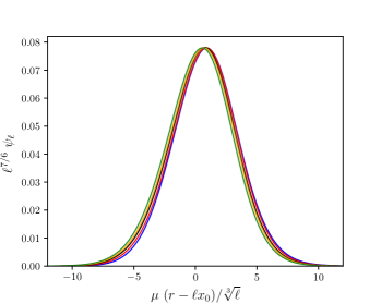
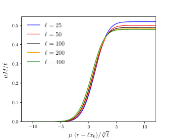
Figure 9: Scaling of the solutions with $\omega=0.8612$, for the quantities $\psi_{\ell}$, $M(r)/\ell$, $\gamma$ and $\alpha$. In these plots, the constant $x_{0}$ appearing on the horizontal axis has been estimated using as reference the $\ell=1600$ configuration with the same $\omega$, using the formula $x_{0}=r_{1600}/1600$, with $r_{1600}$ defined as the location of the maximum of $\psi_{1600}(r)$. The procedure to determine $x_{0}$ without resorting to any particular finite $\ell$ solution is explained in the text.

To describe our scaling method, we consider a family of configurations with increasing value of $\ell$ and fixed $\omega$. As $\ell$ becomes large, the numerical data (see figure 9) suggests that the fields’ profiles depend only on the variable

$$y:=\frac{r-\ell x_{0}}{\ell^{a}},$$ (15)

with $x_{0}$ a positive constant that depends on $\omega$ but not $\ell$, and $a$ a parameter within the range $0<a<1$ that will be determined later. This means that the profiles have their center shifted outwards by $\ell x_{0}$ and stretched by the factor $\ell^{a}$ as $\ell\to\infty$. The fields’ amplitudes are rescaled as follows:

$$M_{*}(y):=\frac{M(r)}{\ell},\qquad\alpha_{*}(y):=\alpha(r)\qquad\gamma_{*}(y):=\gamma(r)\qquad\psi_{*}(y):=\ell^{1+\frac{a}{2}}\psi_{\ell}(r),$$ (16)

the data suggesting that the quantities with a star have finite limits when $\ell\to\infty$. Note that equations (15,16) and the definition of $\gamma$ in equation (4) imply that

$$\gamma_{*}^{-2}(y)=1-\frac{2M_{*}(y)}{x_{0}}\frac{1}{1+\ell^{a-1}\frac{y}{x_{0}}},$$ (17)

such that in the limit $\ell\to\infty$ (with fixed $y$) it follows that $\gamma_{*}^{-2}(y)=1-2M_{*}(y)/x_{0}$. In terms of the rescaled quantities $M_{*}$, $\alpha_{*}$ and $\psi_{*}$ equations (5) can be written as

$$\frac{dM_{*}}{dy}=x_{0}^{2}\left(1+\ell^{a-1}\frac{y}{x_{0}}\right)^{2}\rho_{*},$$ (18a)

$$\frac{1}{\gamma_{*}^{2}\alpha_{*}}\frac{d\alpha_{*}}{dy}=x_{0}\left(1+\ell^{a-1}\frac{y}{x_{0}}\right)p_{r*}+\frac{M_{*}}{x_{0}^{2}}\frac{\ell^{a-1}}{\left(1+\ell^{a-1}\frac{y}{x_{0}}\right)^{2}},$$ (18b)

$$\frac{1}{\alpha_{*}\gamma_{*}}\frac{d}{dy}\left(\frac{\alpha_{*}}{\gamma_{*}}\frac{d\psi_{*}}{dy}\right)+\frac{2}{x_{0}}\frac{\ell^{a-1}}{1+\ell^{a-1}\frac{y}{x_{0}}}\frac{1}{\gamma_{*}^{2}}\frac{d\psi_{*}}{dy}=-\ell^{2a}\left[\frac{\omega^{2}}{\alpha_{*}^{2}}-\mu^{2}-\frac{1}{x_{0}^{2}}\frac{1+\frac{1}{\ell}}{\left(1+\ell^{a-1}\frac{y}{x_{0}}\right)^{2}}\right]\psi_{*},$$ (18c)

where we have introduced the rescaled energy density and radial pressure

$$\rho_{*}(y) := 4\pi\ell^{1+a}\rho(r)=\left(1+\frac{1}{2\ell}\right)\left[\ell^{-2a}\frac{1}{\gamma_{*}^{2}}\left(\frac{d\psi_{*}}{dy}\right)^{2}+\left(\frac{\omega^{2}}{\alpha_{*}^{2}}+\mu^{2}+\frac{1}{x_{0}^{2}}\frac{1+\frac{1}{\ell}}{\left(1+\ell^{a-1}\frac{y}{x_{0}}\right)^{2}}\right)\psi_{*}^{2}\right],$$ (19a)

$$p_{r*}(y) := 4\pi\ell^{1+a}p_{r}(r)=\left(1+\frac{1}{2\ell}\right)\left[\ell^{-2a}\frac{1}{\gamma_{*}^{2}}\left(\frac{d\psi_{*}}{dy}\right)^{2}+\left(\frac{\omega^{2}}{\alpha_{*}^{2}}-\mu^{2}-\frac{1}{x_{0}^{2}}\frac{1+\frac{1}{\ell}}{\left(1+\ell^{a-1}\frac{y}{x_{0}}\right)^{2}}\right)\psi_{*}^{2}\right].$$ (19b)

Let us consider the limiting case $a=0$ first and take the limit $\ell\to\infty$ in these equations (with $y$ held fixed). In this case, one obtains the effective equations

$$\frac{dM_{\infty}}{dy}=x_{0}^{2}\rho_{\infty},\qquad\rho_{\infty}=\frac{1}{\gamma_{\infty}^{2}}\left(\frac{d\psi_{\infty}}{dy}\right)^{2}+\left(\frac{\omega^{2}}{\alpha_{\infty}^{2}}+\mu_{0}^{2}\right)\psi_{\infty}^{2},$$ (20a)

$$\frac{1}{\gamma_{\infty}^{2}\alpha_{\infty}}\frac{d\alpha_{\infty}}{dy}=x_{0}p_{r\infty},\qquad p_{r\infty}=\frac{1}{\gamma_{\infty}^{2}}\left(\frac{d\psi_{\infty}}{dy}\right)^{2}+\left(\frac{\omega^{2}}{\alpha_{\infty}^{2}}-\mu_{0}^{2}\right)\psi_{\infty}^{2},$$ (20b)

$$\frac{1}{\alpha_{\infty}\gamma_{\infty}}\frac{d}{dy}\left(\frac{\alpha_{\infty}}{\gamma_{\infty}}\frac{d\psi_{\infty}}{dy}\right)=-\left(\frac{\omega^{2}}{\alpha_{\infty}^{2}}-\mu_{0}^{2}\right)\psi_{\infty},$$ (20c)

where the index $\infty$ refers to the (pointwise) limit for $\ell\to\infty$, i.e. $M_{\infty}(y)=\lim_{\ell\to\infty}M_{*}(y)$ and similarly for $\alpha_{\infty}$, $\gamma_{\infty}$ and $\psi_{\infty}$. We have also introduced the shorthand notation $\mu_{0}:=\sqrt{\mu^{2}+1/x_{0}^{2}}$ in order to abbreviate the notation. Equations (20) look like a nice system of differential equations for $(M_{\infty},\alpha_{\infty},\psi_{\infty})$ which could be integrated numerically and whose solution with the appropriate boundary conditions should approximate the solution of the full system when $\ell$ is large and $|y|\lesssim\ell$. However, it is not difficult to show that these equations imply that

$$\alpha_{\infty}\gamma_{\infty}p_{r\infty}=\textrm{const},$$ (21)

and by virtue of the boundary conditions this constant must be zero. Therefore, $p_{r\infty}=0$ which implies that $\alpha_{\infty}$ is constant and $\omega^{2}/\alpha_{\infty}^{2}-\mu_{0}^{2}<0$. Then, multiplying both sides of equation (20c) with $\psi_{\infty}$, integrating over $y$ and using integration by parts reveals that $\psi_{\infty}=0$ is the only solution which decays to zero as $y\to\pm\infty$. This indicates that the choice $a=0$ in the rescaling (15) is not the correct one.

Therefore, let us assume that $0<a<1$ is strictly positive and take again the pointwise limit $\ell\to\infty$ in equations (18). This yields

$$\frac{dM_{\infty}}{dy}=x_{0}^{2}\rho_{\infty},\qquad\rho_{\infty}=\left(\frac{\omega^{2}}{\alpha_{\infty}^{2}}+\mu_{0}^{2}\right)\psi_{\infty}^{2},$$ (22a)

$$\frac{1}{\gamma_{\infty}^{2}\alpha_{\infty}}\frac{d\alpha_{\infty}}{dy}=x_{0}p_{r\infty},\qquad p_{r\infty}=\left(\frac{\omega^{2}}{\alpha_{\infty}^{2}}-\mu_{0}^{2}\right)\psi_{\infty}^{2},$$ (22b)

while the rescaled Klein-Gordon equation (18c) implies that $p_{r\infty}$ must vanish in order for the right-hand side to be finite. It follows that

$$\alpha_{\infty}=\frac{\omega}{\mu_{0}}$$ (23)

is constant and that

$$\frac{dM_{\infty}}{dy}=2x_{0}^{2}\mu_{0}^{2}\psi_{\infty}^{2}=2(1+\mu^{2}x_{0}^{2})\psi_{\infty}^{2}.$$ (24)

The problem is that (so far) we have no differential equation for $\psi_{\infty}$. However, a differential equation for $\psi_{\infty}$ can be obtained by expanding the rescaled fields:

$$\psi_{*}(y)=\psi_{\infty}(y)+\varepsilon\psi_{1}(y)+{\cal O}(\varepsilon^{2}),$$ (25)

and similarly for $M_{*}$ and $\alpha_{*}$ in powers of $\varepsilon=\varepsilon(\ell)$ and looking at the next-order contributions from equations (18). For the following, we choose $\varepsilon(\ell)=\ell^{a-1}$ since most of these corrections terms are of this order, and we expand the rescaled lapse in the form

$$\alpha_{*}(y)=\alpha_{\infty}\left[1+\ell^{a-1}\delta(y)+{\cal O}(\ell^{-1})\right],$$ (26)

with the function $\delta(y)$ describing the first-order correction. Using equation (23) the right-hand side of equation (18c) gives, to leading order in $1/\ell$,

$$2\ell^{3a-1}\left(\mu_{0}^{2}\delta-\frac{y}{x_{0}^{3}}\right)\psi_{\infty},$$ (27)

which yields a finite contribution if $a=1/3$. Choosing $a=1/3$ in the expansion (26), equations (18b,18c) yield the two differential equations

$$\frac{1}{\gamma_{\infty}^{2}}\frac{d\delta}{dy} = x_{0}\left[\frac{1}{\gamma_{\infty}^{2}}\left(\frac{d\psi_{\infty}}{dy}\right)^{2}-2\left(\mu_{0}^{2}\delta-\frac{y}{x_{0}^{3}}\right)\psi_{\infty}^{2}\right]+\frac{M_{\infty}}{x_{0}^{2}},$$ (28a)

$$\frac{1}{\gamma_{\infty}}\frac{d}{dy}\left(\frac{1}{\gamma_{\infty}}\frac{d\psi_{\infty}}{dy}\right) = 2\left(\mu_{0}^{2}\delta-\frac{y}{x_{0}^{3}}\right)\psi_{\infty},$$ (28b)

which can be integrated along with equation (24) and $\gamma_{\infty}^{-2}=1-2M_{\infty}/x_{0}$ in order to find $(M_{\infty},\delta,\psi_{\infty})$. Note that the expression inside the square parenthesis on the right-hand side of equation (28a) is the $\ell^{-2/3}$-contribution to $p_{r*}$.

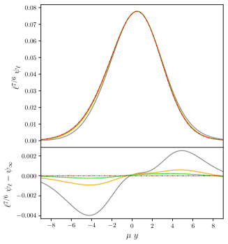
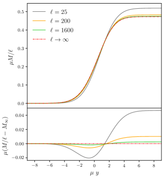
Figure 10: Solutions with $\ell\gg 1$ compared to the same $\omega=0.8612$ solution obtained from the effective ($\ell\to\infty$ limit) equations (24,28). The asymptotic solution $\ell\to\infty$ yields the value $x_{0}=2.73$. In the bottom panels we show the difference between the finite $\ell$ configurations and the $\ell\to\infty$ case, which converges to zero.

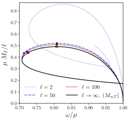
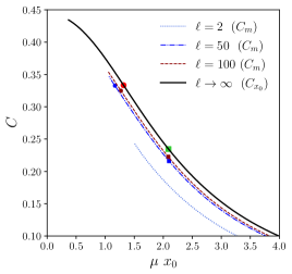
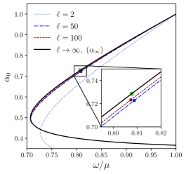
Figure 11: Equilibrium $\ell\gg 1$ configurations. Left panel: Total mass vs. the frequency $\omega/\mu$. Center panel: Compactness $C_{x_{0}}$ for the $\ell\to\infty$ limit. Right panel: Minimum of the lapse $\alpha_{0}=\alpha(r=0)$ vs. $\omega/\mu$. The green square represents the maximum ($\ell\to\infty$) configuration and the red circle denotes the first appearance of light rings, at $C_{x_{0}}=1/3$.

The rescaled equations (24,28) are solved on a finite interval $[y_{L},y_{R}]$ with $y_{L}<0<y_{R}$, fixing the left boundary conditions $M_{*}=0$, $\delta=0$, $\psi_{*}=\psi_{*L}$ at $y=y_{L}$ and the right boundary condition $\psi_{*}\sim 0$ at $y=y_{R}$. The integration is carried out by means of a shooting method from left to right, where $\psi_{*}$ is fixed at $y_{L}$ and the value of $x_{0}$ for which the field matches the boundary condition at $y_{R}$ is searched for. In this procedure, it is necessary to provide the value of $d\psi_{*}/dy$ at $y_{L}$ given $\psi_{*L}$; this can be done by studying the asymptotic behavior $y\to-\infty$ of the rescaled equations. It is obtained that the scalar field takes the form $\psi_{*}\propto\mathrm{Ai}(z)\approx\exp(-\frac{2}{3}z^{3/2})/z^{1/4}$ with $z=-\sqrt[3]{2}y/x_{0}$ and $\mathrm{Ai}$ the Airy function of the first kind, obtaining $d\psi_{*}/dy\approx(\sqrt{-2y/x_{0}^{3}}-1/(4y))\psi_{*}$.

After $x_{0}$ is found, the total mass of the solution is obtained by evaluating $M_{\infty T}:=M_{\infty}(y=y_{R})$. Outside the spherical shell, at $y=y_{R}$, we evaluate $\alpha_{\infty}=1/\gamma_{\infty}(y_{R})$ and calculate $\omega$ from equation (23). Once the pair $(\omega,x_{0})$ is obtained from the effective equations, we can compare the fields with those corresponding to the same $\omega$ finite $\ell$ solutions. Notice that there is no loss in generality in choosing $\delta(y_{L})=0$ since the system (24,28) is invariant under the transformation $(y,\delta)\mapsto(y-\zeta,\delta-\zeta/(\mu_{0}^{2}x_{0}^{3}))$ with $M_{\infty}$ and $\psi_{\infty}$ unchanged. In fact, as the lower right panel of figure 9 shows, the $\delta$ correction to $\alpha$ is not zero in the inner shell region. In turn, the previous transformation will translate horizontally the scalar field profile. So there are two ways to calculate $\zeta$, the first is to take a solution with large $\ell$ and find the value of the $\delta$ correction within the shell, the second is to use the scalar field profile and make the maxima of $\psi_{*}$ of the large $\ell$ solution and the effective $\ell\to\infty$ solution to overlap; these two forms are equivalent.

We illustrate the fields’ rescaling in figure 10, showing convergence to the limiting $\ell\rightarrow\infty$ case, as expected. We have found that the value of $x_{0}$ that corresponds to a solution with the frequency of the previous (stable branch) figure 9 configurations, $\omega=0.8612$, is $x_{0}=2.73$. The estimated value for the $\alpha$ correction in this case is $\zeta=2.17$. It is found that for this $\zeta$ value, the maxima of $\psi_{*}$ overlap, as expected. Figure 11 shows a plot for certain global quantities of the equilibrium solutions of the rescaled $\ell\to\infty$ limit. The left panel shows that a critical mass solution, $M_{\infty T}=0.49031$, is obtained at $\omega=0.8077$ (marked with a green square). This solution is obtained for the values $x_{0}=2.0902$ and $\zeta=1.58$.

Next, we evaluate the anisotropy and compactness of this particular configuration. In contrast to the rescaled radial pressure (19b), the rescaled tangential pressure

$$p_{T*}(y):=4\pi\ell^{1+a}p_{T}=\left(1+\frac{1}{2\ell}\right)\left[-\ell^{-2a}\frac{1}{\gamma_{*}^{2}}\left(\frac{d\psi_{*}}{dy}\right)^{2}+\left(\frac{\omega^{2}}{\alpha_{*}^{2}}-\mu^{2}\right)\psi_{*}^{2}\right],$$ (29)

does not vanish in the pointwise $\ell\to\infty$ limit:

$$p_{T\infty}=\left(\frac{\omega^{2}}{\alpha_{\infty}^{2}}-\mu^{2}\right)\psi_{\infty}^{2}=\frac{\psi_{\infty}^{2}}{x_{0}^{2}},$$ (30)

which is consistent with the observations made in section III.2.

We show in figure 12 a plot for the tangential pressure as well as the rescaled energy density, equation (22a), for the solution of maximum mass.

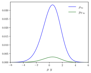
Figure 12: Rescaled energy density and tangential pressure for the $\ell\to\infty$ maximum mass solution. Notice that $p_{T}$ is always positive, while $p_{r}$ is strictly zero in this limit.

Now, to determine the compactness of these solutions, the easiest way is to note that the quotient $M(r)/r$ in terms of the rescaled quantities in equations (15,16), reduces to $M_{\infty}(y)/x_{0}$ in the $\ell\to\infty$ limit, allowing us to define,

$$C_{x_{0}}:=\frac{M_{\infty T}}{x_{0}}.$$ (31)

In the central panel of figure 11 we show the $x_{0}$ value of the solution as a function of the compactness $C_{x_{0}}$ (and $C_{m}$ for the finite $\ell$ solutions). For the maximum mass solution, the compactness obtained is $C_{x_{0}}=0.234554$. Like the finite $\ell$ solutions, the compactness increases as the value of the boson star radius decreases, approaching the limit value of $0.5$. However, the $\ell=\infty$ solutions with compactness exceeding $\simeq 0.433$ have frequencies $\omega$ larger than $\mu$, and thus they do not correspond to a limit of solutions with finite $\ell$ which must have $\omega/\mu<1$ due to the exponential decay of the scalar field at spatial infinity.

Next, we wonder about the presence of light rings for the $\ell\gg 1$ configurations. As stated above, the existence of these rings is given by the existence of local extrema of $V_{\mathrm{eff}}$. For large $\ell$ the effective potential for null geodesics is

$$V_{\mathrm{eff}}(r)=L^{2}\frac{\alpha^{2}}{r^{2}}=\frac{L^{2}}{\ell^{2}}\frac{\alpha_{\infty}^{2}}{x_{0}^{2}}\left[1+\frac{2}{\ell^{2/3}}\left(\delta(y)-\frac{y}{x_{0}}\right)+{\cal O}\left(\frac{1}{\ell}\right)\right].$$ (32)

For the following it is convenient to introduce the rescaled potential $V_{1}$, defined as

$$V_{1}(y):=\ell^{2/3}\left(\frac{x_{0}^{2}}{\alpha_{\infty}^{2}}\frac{\ell^{2}}{L^{2}}V_{\mathrm{eff}}(r)-1\right)=2\left(\delta(y)-\frac{y}{x_{0}}\right)+{\cal O}\left(\frac{1}{\ell^{1/3}}\right).$$ (33)

Figure 13 shows the function $V_{1}(y)$ for $\ell=50$ and $\ell=100$ along with the $\ell\rightarrow\infty$ limit. Starting from the knowledge of $\delta(y)$ we can obtain the approximate location of $r_{\mathrm{in}}$, the inner light ring for $\ell\gg 1$ solutions. However, as shown in figure 13 at this order one is unable to determine the position of the outer ring which moves away from $y=0$ as $\ell$ increases; in fact, it seems that the location of this second light ring diverges to $y\to\infty$ when $\ell\to\infty$.

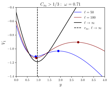
Figure 13: Effective rescaled potential $V_{1}$ for circular null geodesics for $\ell=50,100$ solutions together with the $\ell\rightarrow\infty$ case. The circles indicate the position of the light rings.

Evaluating the condition $dV_{1}/dy=0$ along the $\ell\rightarrow\infty$ family of configurations we obtain that the solution closest to the critical mass point satisfying this condition for some value of $y$, is the one that has compactness $C_{x_{0}}=1/3$ (red dot in figure 11). This correspond to the solution with $x_{0}=1.32$ and $\omega=0.7251$.

To close the discussion of this section on the rescaling properties for large $\ell$, we list the transformations involving certain relevant quantities mentioned in the previous paragraphs. To do this, suppose the situation in which an $\ell$-boson star solution has been obtained for a certain value of $\omega$ and sufficiently large $\ell=\ell_{1}$; then starting from it we can obtain an approximate solution with arbitrarily large $\ell=\ell_{2}>\ell_{1}$ for the same $\omega$ in the following way: first, identify the position $r$ of the maximum of $\psi_{\ell}$ and estimate $x_{0}=r/\ell_{1}$. Then, apply the transformation $r\mapsto\sqrt[3]{\ell_{2}/\ell_{1}}(r-\ell_{1}x_{0})+\ell_{2}x_{0}$. As function of this redefined coordinate $r$, the amplitude of the scalar field becomes smaller according to $\psi_{\ell_{1}}(r)\mapsto\psi_{\ell_{2}}(r)=(\ell_{1}/\ell_{2})^{7/6}\psi_{\ell_{1}}(r)$ while the mass function grows as $M(r)\mapsto(\ell_{2}/\ell_{1})M(r)$. The energy density and the tangential pressure both decrease according to $\rho(r)\mapsto(\ell_{1}/\ell_{2})^{4/3}\rho(r)$ and $p_{T}(r)\mapsto(\ell_{1}/\ell_{2})^{4/3}p_{T}(r)$. On the other hand, the mass, radius and compactness parameters rescale as follows: $(M_{T},R_{99},C_{99})\mapsto(\ell_{2}/\ell_{1}M_{T},\ell_{2}/\ell_{1}R_{99},C_{99})$ and $(M_{m},R_{m},C_{m})\mapsto(\ell_{2}/\ell_{1}M_{m},\ell_{2}/\ell_{1}R_{m},C_{m})$. Let this example above serve as an illustration of the rescaling properties; certainly a better way to obtain a solution with $\ell=\ell_{2}$ is to solve the effective equations and then obtain the quantities with finite $\ell$ by inverting the definitions of the rescaled variables. In this case the error would be of order $\ell_{2}^{-2/3}$ or even smaller for some of the quantities.

V Conclusions

We have studied various properties of the recently introduced $\ell$-boson stars Alcubierre et al. (2018), analyzing in each case the role played by the angular momentum parameter $\ell$, and paying particular attention to the large $\ell$ regime. These objects are composed of $2\ell+1$ massive complex scalar fields and present notable characteristics which single them out from the standard $\ell=0$ boson stars, while still sharing with them several common features Alcubierre et al. (2018, 2019, 2021); Jaramillo et al. (2020); Sanchis-Gual et al. (2021). Among these features are the fact that both are formed with complex scalar fields on a spherically symmetric spacetime; they both admit diluted and compact solutions; and they possess stable and unstable branches separated by the solution of maximum mass for a given $\ell$. On the other hand, we had previously Alcubierre et al. (2018, 2019, 2021) observed some characteristics related to the $\ell$ parameter: an increase in the compactness and size of the maximum mass configurations and the fact that their morphology tends to form a hollow-like central region (even in the $\ell=1$ boson star case), with the position of the maximum of density moving away from $r=0$. The purpose of the present work was to take a step forward and perform a thorough examination of how these features change with $\ell$. In particular, using different numerical methods, we were able to increase notably the magnitude of the parameter $\ell$ and finally, with the information of $\ell\gg 1$ solutions and a careful analysis of the system of equations, we were able to study the limiting case when the parameter $\ell$ goes to infinity.

One of the interesting features that can be observed is the fact that for $\ell>1$ the density in the central region is much smaller than in the shell region. We have shown in this work that, as $\ell$ grows, so does the object and also the almost empty central region, tending to form shells of scalar fields where the size of the almost empty central region is much larger than the size of the region where the scalar field is mainly distributed. This tendency in the behavior goes all the way to infinity, making the objects look like larger and larger shells. We have shown that, when $\ell\gg 1$ the scalar field profile is shifted outwards proportionally to $\ell$ while its width grows as $\sqrt[3]{\ell}$. Furthermore, the spatial components of the stress energy-momentum tensor tend to be highly anisotropic as $\ell$ increases. Indeed, as $\ell$ grows the radial pressure tends to zero, while the tangential one remains finite. In this way, for large values of $\ell$, the shells tend to have no radial pressure and are supported solely by the tangential ones, analogous to the way in which a Roman arch supports its own weight. This increase in the anisotropy seems related to an increase in the compactness Dev and Gleiser (2002) of the $\ell$-boson star. The mass of the solutions that divide the stable and the unstable branches, as well as their size, grows with $\ell$, but in such a way that the compactness tends to a finite value. We have proven that in the $\ell\rightarrow\infty$ limit the compactness tends to about $0.23$ for the maximum mass configuration; that is, about half the Buchdahl limit. However, unstable configurations may be much more compact, reaching a compactness of about $0.433$ in the large $\ell$ limit. In this regard, it is interesting to point out that (single and multiple) shell-type configurations have also been found when analyzing the spherically symmetric steady-state solutions of the Einstein-Vlasov system Andreasson and Rein (2007). In particular, it has been proven that such shells satisfy the Buchdahl inequality and that static shells of Vlasov matter can have $M(r)/r$ arbitrarily close to $4/9$ Andreasson (2007, 2008).

Regarding orbiting particles, the high compactness that $\ell$-boson stars can achieve while remaining stable gives rise to new features, which differentiate them from standard boson stars and also from black holes. Schwarzschild black holes have an ISCO located at $6M$, with no stable circular orbits below that value. Consequently, accretion disks around non-rotating black holes typically have an inner boundary and “end” at $r=6M$. Stable standard boson stars do not have ISCOs, meaning that they could in principle possess an accretion disk extending all the way to the star’s center. On the other hand, stable $\ell$-boson stars exist with an ISCO-OSCO pair. In this case, accretion disks could show a “gap” between the ISCO and OSCO, to then again extend all the way to the center. These differences could constitute an important observable feature.

Besides causal circular orbits, we studied null ones, also known as light rings. We found that, for each $\ell$, a pair of light rings appears at high enough compactness, the exterior one beeing unstable and the interior one stable. These light rings are always in the unstable spacetime regions, although they begin appearing closer and closer to the stable region as $\ell$ increases, which seems reasonable given that more compact stable solutions exist for larger $\ell$. Our findings are consistent with the results of Cunha et al. (2017): if a regular compact object has a light ring, it must have at least two, one of them being stable; and the presence of the stable light ring is expected to lead to nonlinear spacetime instabilities.

In our vast parameter exploration we have not included excited modes (higher frequency solutions containing one or more nodes of $\psi_{\ell}$), which would be unstable if results for standard boson stars also hold here Balakrishna et al. (1998). However, solutions that combine a stable ground state solution with excited ones might again be stable Bernal et al. (2010). We expect to address these questions in future works.

Apart from the properties discussed in this article, $\ell$-boson stars open up the possibility to consider a larger landscape of solutions such as the ones described in Sanchis-Gual et al. (2021). These results along with the existence of a stable branch for the $\ell$-boson stars Alcubierre et al. (2019, 2021); Jaramillo et al. (2020) make us conclude that such localized bosonic systems may play an important role in modeling astrophysical objects, such as galactic halos or black hole mimickers with potential observable consequences. Further work along these lines is underway and will be presented in the near future.

Appendix A Definitions and rescaling in $\mu$

We include tables that provide summarized information in a single place, aiding in the reading of this article. A summary of the main definitions used in this work is shown in Table 1. Rescaling rules in $\mu$, which allows one to obtain solutions for arbitrary $\mu$ from the solution of any given $\mu_{0}$, are shown in Table 2.

Table 1: Summary of the main definitions used in this article.

Symbol	Definition	Depends on
$M$	Mass function, also $M(r)$	$\ell$, $u_{0}$, $r$
$M_{T}$	Total mass (or mass function at outer boundary)	$\ell$, $u_{0}$
$R_{99}$	Areal radius containing 99% of the total mass	$\ell$, $u_{0}$
$C_{99}$	$M_{T}/R_{99}$	$\ell$, $u_{0}$
$C_{m}$	Maximum of $M(r)/r$ over $r>0$	$\ell$, $u_{0}$
$R_{m}$	Location of maximum $M(r)/r$	$\ell$, $u_{0}$
$M_{m}$	Mass function evaluated at $R_{m}$	$\ell$, $u_{0}$
$r_{\rm in}$	Location of the inner light ring	$\ell$, $u_{0}$
$r_{\rm out}$	Location of the outer light ring	$\ell$, $u_{0}$
$r_{\rm osco}$	Location of the OSCO	$\ell$, $u_{0}$
$r_{\rm isco}$	Location of the ISCO	$\ell$, $u_{0}$
$M_{\rm max}$	Maximum of $M_{T}$ (for a given $\ell$)	$\ell$

Table 2: Solutions for arbitrary values of $\mu$ can be obtained from those of a given value by performing a rescaling as shown in this table.

$\mu$	$\mapsto$	$\lambda\,\mu$
($\alpha$, $\gamma$, $\psi_{\ell}$)	$\mapsto$	($\alpha$, $\gamma$, $\psi_{\ell}$)
$u_{0}$	$\mapsto$	$\lambda^{\ell}\,u_{0}$
$\omega$	$\mapsto$	$\lambda\,\omega$
($r$, $M$)	$\mapsto$	$\lambda^{-1}$ ($r$, $M$)
($\rho$, $p_{r}$, $p_{T}$)	$\mapsto$	$\lambda^{2}$ ($\rho$, $p_{r}$, $p_{T}$)

Appendix B Numerical methods

We obtain solutions of the eigenvalue problem in equations (5) numerically using two different methods, implemented in independent codes. For $\ell\lesssim 25$ we use a shooting method similar to the one described in our previous work Alcubierre et al. (2018), but with some improvements. For larger $\ell$ it becomes more and more difficult for this code to converge to a given mode. In those cases we switch instead to a spectral method. These methods, which are described in the following subsections, give the same results in the parameter region where both are able to obtain solutions.

B.1 Shooting Method

To obtain solutions for $\ell\lesssim 25$ we use a “shooting to a fitting point method” based on Press et al. (1986), implemented in a code which is described in Megevand et al. (2007). It consist of doing a direct numerical integration of the ordinary differential equations starting both from the left and right boundaries, at which one imposes either appropriate physical conditions or guesses when those are undetermined, with the goal of matching both the fields and their first derivatives at some intermediate point. This defines a function of the mentioned guesses, plus an additional guess, the eigenvalue $\omega^{2}$, whose roots correspond to the fitting condition being satisfied. In order to find such roots, a Newton-Raphson method is used. The fitting point method is particularly useful when one has a system with a pair of solutions, one rapidly growing and the other rapidly decreasing at each boundary, and one wants to obtain the (physical) solution that decays to zero at both boundaries, as in the large $\ell$ cases. For the numerical integration, instead of the algorithm described in Press et al. (1986), we use a more sophisticated step adaptive method provided by the LSODE routines Radhakrishnan and Hindmarsh (1993). For the particular applications of this work, it was also helpful in a few cases to modify the left boundary conditions in order to be able to set them at locations quite a bit to the right of $r=0$. This is due to the shell-like shape of the stars for large enough $\ell$. The details are given below. Finally, even though the solutions for a given value of $\mu$ can be trivially obtained from a rescaling of the $\mu=1$ case (see appendix A), which is the value we fixed in most situations, sometimes it helped the numerical code to easily find solutions to vary $\mu$ depending on the particular region of the parameter space. This is because some fields may become many orders of magnitude different when one restricts oneself to the $\mu=1$ case. Nevertheless, we present all our results in a $\mu$ independent form.

B.1.1 Approximate solutions for low density

As mentioned throughout the article, for large values of $\ell$ the scalar field distribution is shell-like, with very low density (as compared to its maximum value) in an interior region with $r<r_{1}$ and in an exterior region with $r_{2}<r$ for certain values $r_{1}<r_{2}$. In the interior region the solutions can be approximated by those of a scalar field on a flat spacetime, while in the exterior region they can be approximated by solutions of a scalar field on a Schwarzschild spacetime with mass $M_{T}$.

In the interior region ($r<r_{1}$) we can assume $\alpha=\gamma=1$. Then, from equation (5c), we get

$$\frac{1}{r^{2}}\left(r^{2}\psi_{\rm in}^{\prime}\right)^{\prime}=\left(\mu^{2}-\omega^{2}+\frac{\ell(\ell+1)}{r^{2}}\right)\psi_{\rm in},$$ (34)

with solutions

$$\psi_{\rm in}(r)=C_{1}\frac{J_{\ell+\frac{1}{2}}\left(\sqrt{\omega^{2}-\mu^{2}}\,r\right)}{\sqrt{r}}+C_{2}\frac{Y_{\ell+\frac{1}{2}}\left(\sqrt{\omega^{2}-\mu^{2}}\,r\right)}{\sqrt{r}},$$ (35)

where $J_{\nu}(x)$ and $Y_{\nu}(x)$ are the Bessel functions of the first and second kind, respectively. Keeping only the solution with the proper behavior at $r=0$ and writing the arbitrary amplitude in terms of $u_{0}$ we obtain

$$\psi_{\rm in}(r)=u_{0}\,\frac{2^{\left(\ell+\frac{1}{2}\right)}\,\Gamma\left(\ell+\frac{3}{2}\right)}{{\left(\sqrt{\omega^{2}-\mu^{2}}\right)}^{\ell+\frac{1}{2}}}\,\frac{J_{\ell+\frac{1}{2}}\left(\sqrt{\omega^{2}-\mu^{2}}\,r\right)}{\sqrt{r}}.$$ (36)

In order to transform to the gauge used in the remainder of this work, in which $\alpha=1$ at $r=\infty$, rather than at $r=0$, one just needs to replace $\omega$ with $\gamma_{\infty}\,\alpha_{\infty}\,\omega$ in equation (36). We show an example of this approximation in figure 14. We see a very good agreement between the scalar field and its approximation even well beyond $\mu\,r=\mu\,r_{1}\approx 40$.

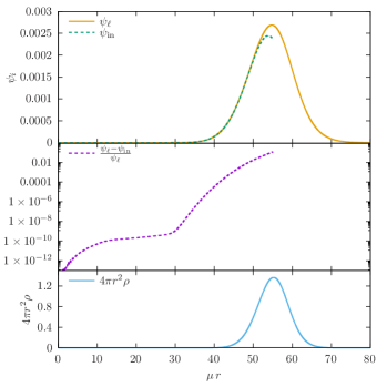
Figure 14: Solution $\psi_{\ell}$ and approximation $\psi_{\textnormal{in}}$ for the case with $\ell=25$ and maximum mass $M_{T}=13.45$ (top panel). The middle panel shows the relative error. For reference we also include the density profile in the bottom panel.

Finally, we note that in the exterior region one can assume the metric is given by a Schwarzschild solution with mass $M_{T}$. Then, the scalar field can be expressed in terms of the confluent Heun functions. However, we did not use the external region approximations in this paper, hence we will not present any details here.

B.2 Spectral Method

An independent code was built based on a multidomain spectral method. Specifically, a collocation method has been used with Chebyshev polynomials as the basis functions. Details of the code described in the following paragraphs were essentially implemented based on Grandclément and Novak (2009) which is a review on spectral methods in numerical relativity. The Einstein-Klein-Gordon equations were solved in isotropic coordinates, where the differential operators in the resulting equations in the system are similar to each other and therefore easier to implement in this particular method.

The physical domain, parametrized by the radial coordinate is decomposed into 5 carefully placed domains depending on what range of solutions we want to obtain in a single run, given $\ell$. For the outer domain a compactification is carried out so that the external boundary conditions can be imposed at spatial infinity. On the other hand, in the domain that contains the origin, an even base of Chebyshev polynomials is used for the lapse and the conformal factor $\Psi$, while an even (odd) base is used for the field if $\ell$ is even (odd), which guarantee the solution is regular at the origin. The non-linear system of equations that results for the coefficients of the expansion is solved iteratively using a Newton scheme, the extra variable $\omega$ is compensated with an extra equation $\alpha(r=0)=\alpha_{0}>0$, which ensures that the code does not converge to the trivial solution.

An initial guess is required in the Newton scheme for the coefficients of the expansion in all the functions (as well as the frequency), this is equivalent to provide an initial guess for the functions. Given certain value of $\ell$, the first solution is obtained from reasonable choices for the three parameters, $\sigma$, $r_{0}$ and $\phi_{0}$, which control the properties of the following simple initial guess

$$\psi_{\ell} =\left(\frac{\bar{r}}{r_{0}}\right)^{\ell}\phi_{0}\exp\left(-\frac{\bar{r}^{2}-r_{0}^{2}}{\sigma^{2}}\right),$$ (37)

$$\alpha =-(1-\alpha_{0})\exp(-\bar{r}^{2})+1,$$ (38)

$$\Psi =1.$$ (39)

Here $\bar{r}$ refers to the isotropic radial coordinate. The solutions are easier to find in the Newtonian regime where the frequency is close to one. For example, in the $\ell=50,\ 100$ cases presented here we start with an initial guess of $\omega=0.95$ and once the first solution is obtained we slightly decrease the value of $\alpha_{0}$ and take as the new initial guess the previous solution.

We have checked that in the spectral code, as in the convergence test performed in Grandclément et al. (2014) for the $\ell=0$ case, the error indicators, as for example the frequency and the difference of the ADM and Komar masses converge exponentially to a fixed value and to zero respectively, as we increase the number of Chebyshev basis polynomials, as expected for a spectral method.

Appendix C Summary of numerical data

Table 3 shows information regarding most of the solutions analyzed in this paper.

Table 3: Properties of some of the solutions obtained in this work. For each $\ell$ (and $\mu$), the ground state solution is uniquely determined by fixing one more parameter, like $u_{0}$ or $\alpha_{0}$. We mainly use $u_{0}$ for small $\ell$ and $\alpha_{0}$ for large $\ell$. Hence, in most cases, we only report one of these parameters. In the column titled “stable”, “m.s.” stands for marginally stable, corresponding to solutions of maximum total mass, which define the transition point between stable and unstable solutions. In the $\ell=\infty$ case (marked with ^†), m.s. simply indicates the maximum mass solution. Also in the $\ell=\infty$ case, the total mass values (indicated with ^⋆) actually correspond to the mass rescaled with $\ell$ as in section IV, since otherwise those values are not finite.

$\ell$	$u_{0}/\mu^{\ell}$	$\alpha_{0}$	$\omega/\mu$	$\mu M_{T}$	$\mu M_{m}$	$\mu R_{99}$	$\mu R_{m}$	$C_{99}$	$C_{m}$	$\mu r_{\rm in}$	$\mu r_{\rm out}$	$\mu r_{\rm osco}$	$\mu r_{\rm isco}$	stable	Figure
0	1.30e-2		0.9911	0.229	0.1707	41.908	22.332	0.0055	0.0076	–	–	–	–	yes	1,2,4,5,6,8,9,10,11,12,14
0	2.71e-1		0.8530	0.633	0.4587	7.855	3.815	0.0806	0.1202	–	–	–	–	m.s.	1,2,4,5,6,8,9,10,11,12,14
0	2.20e+0		0.8428	0.374	0.0016	5.043	0.006	0.0742	0.2581	0.0031	0.0082	0.0031	0.013	no	1,2,4,5,6,8,9,10,11,12,14
1	5.00e-4		0.9864	0.489	0.4041	47.763	32.090	0.0102	0.0126	–	–	–	–	yes	1,2,4,5,6,8,9,10,11,12,14
1	4.00e-3		0.9487	0.875	0.7233	23.115	15.460	0.0379	0.0468	–	–	–	–	yes	1,2,4,5,6,8,9,10,11,12,14
1	3.35e-2		0.8353	1.176	0.9650	10.157	6.590	0.1158	0.1464	–	–	–	–	m.s.	1,2,4,5,6,8,9,10,11,12,14
1	5.01e-1		0.8384	0.543	0.3739	3.860	1.224	0.1407	0.3056	1.1057	1.1191	1.1057	2.99	no	1,2,4,5,6,8,9,10,11,12,14
1	1.60e+0		0.8742	0.702	0.1504	7.333	0.430	0.0958	0.3500	0.2947	0.5691	0.2947	0.952	no	1,2,4,5,6,8,9,10,11,12,14
1	2.50e+0		0.8603	0.670	0.1008	6.183	0.280	0.1084	0.3596	0.1875	0.3936	0.1875	0.603	no	1,2,4,5,6,8,9,10,11,12,14
1	7.00e+0		0.8883	0.613	0.0376	6.579	0.102	0.0932	0.3690	0.0666	0.1542	0.0666	0.213	no	1,2,4,5,6,8,9,10,11,12,14
5	1.00e-10		0.9757	1.686	1.5377	72.612	61.560	0.0232	0.0250	–	–	–	–	yes	1,2,4,5,6,8,9,10,11,12,14
5	5.00e-7		0.8165	3.293	3.0197	19.470	16.628	0.1691	0.1816	–	–	–	–	m.s.	1,2,4,5,6,8,9,10,11,12,14
5	3.40e-3		0.9016	1.314	1.1984	4.037	3.282	0.3255	0.3651	2.76	3.90	2.76	7.87	no	1,2,4,5,6,8,9,10,11,12,14
25	4.67e-53		0.9499	9.265	8.9616	162.304	156.420	0.0571	0.0573	–	–	–	–	yes	1,2,4,5,6,8,9,10,11,12,14
25	4.67e-47		0.8826	12.490	12.1047	95.484	92.363	0.1308	0.1311	–	–	–	–	yes	1,2,4,5,6,8,9,10,11,12,14
25	1.03e-42		0.8091	13.451	13.0691	64.363	62.556	0.2090	0.2089	–	–	64.8	80.55	m.s.	1,2,4,5,6,8,9,10,11,12,14
25	1.87e-36		0.7167	11.488	11.2098	35.994	35.251	0.3192	0.3180	–	–	35.055	68.85	no	1,2,4,5,6,8,9,10,11,12,14
25	9.35e-30		0.7608	7.425	7.2693	19.263	18.969	0.3855	0.3832	17.601	22.275	17.601	44.55	no	1,2,4,5,6,8,9,10,11,12,14
25	1.08e-45	0.8	0.8612	12.980	12.5892	84.434	81.799	0.1537	0.1539	–	–	–	–	yes	1,2,4,5,6,8,9,10,11,12,14
50	1.00e-94	0.72277	0.8088	25.942	25.5042	119.187	118.120	0.2177	0.2159	–	–	120.1	152.0	m.s.	1,2,4,5,6,8,9,10,11,12,14
50	1.00e-99	0.80343	0.8612	25.004	24.5308	156.170	154.380	0.1601	0.1589	–	–	–	–	yes	1,2,4,5,6,9,1,11,11,12,14
100	1.00e-216	0.72331	0.8073	50.756	50.2279	225.660	225.660	0.2249	0.2226	–	–	227.1	298.0	m.s.	1,2,4,5,6,8,9,10,11,12,14
100	1.00e-220	0.80513	0.8612	48.911	48.8731	296.630	296.630	0.1648	0.1631	–	–	–	–	yes	1,2,4,5,6,8,9,10,11,12,14
200		0.8065	0.8612	96.510	95.8531	575.580	577.070	1.6767	0.1661	–	–	–	–	yes	1,2,4,5,6,8,9,10,11,12,14
400		0.80725	0.8612	191.452	190.6695	1128.450	1132.820	0.1697	0.1683	–	–	–	–	yes	1,2,4,5,6,8,9,10,11,12,14
1600		0.808	0.8612	759.695	758.6214	4422.320	4437.550	0.1718	0.1710	–	–	–	–	yes	1,2,4,5,6,8,9,10,11,12,14
$\infty$		0.8086	0.8612	$0.472^{\star}$				0.1730							1,2,4,5,6,8,9,10,11,12,14
$\infty$		0.7286	0.8077	$0.490^{\star}$				0.2346						m.s.†	1,2,4,5,6,8,9,10,11,12,14
$\infty$		0.5773	0.7251	$0.439^{\star}$				0.3333							1,2,4,5,6,8,9,10,11,12,14

References

- Preskill et al. (1983) J. Preskill, M. B. Wise, and F. Wilczek, Phys. Lett. B120, 127 (1983).
- Abbott and Sikivie (1983) L. F. Abbott and P. Sikivie, Phys. Lett. B120, 133 (1983).
- Dine and Fischler (1983) M. Dine and W. Fischler, Phys. Lett. B120, 137 (1983).
- Zyla et al. (2020) P. A. Zyla et al. (Particle Data Group), PTEP 2020, 083C01 (2020).
- Marsh (2016) D. J. E. Marsh, Phys. Rept. 643, 1 (2016), eprint 1510.07633.
- Hui et al. (2017) L. Hui, J. P. Ostriker, S. Tremaine, and E. Witten, Phys. Rev. D95, 043541 (2017), eprint 1610.08297.
- Niemeyer (2019) J. C. Niemeyer (2019), eprint 1912.07064.
- Hu et al. (2000) W. Hu, R. Barkana, and A. Gruzinov, Phys. Rev. Lett. 85, 1158 (2000), eprint astro-ph/0003365.
- Matos et al. (2000) T. Matos, F. S. Guzman, and L. A. Ureña López, Class. Quantum Grav. 17, 1707 (2000), eprint astro-ph/9908152.
- Matos and Ureña López (2001) T. Matos and L. A. Ureña López, Phys. Rev. D63, 063506 (2001), eprint astro-ph/0006024.
- Matos et al. (2008) T. Matos, A. Bernal, and D. Núñez, Rev.Mex.A.A. 44, 149 (2008), eprint astro-ph/0303455.
- Genina et al. (2018) A. Genina, A. Benítez-Llambay, C. S. Frenk, S. Cole, A. Fattahi, J. F. Navarro, K. A. Oman, T. Sawala, and T. Theuns, Monthly Notices of the Royal Astronomical Society 474, 1398 (2018).
- Kendall and Easther (2020) E. Kendall and R. Easther, Publ. Astron. Soc. Austral. 37, e009 (2020), eprint 1908.02508.
- Kim et al. (2018) S. Y. Kim, A. H. G. Peter, and J. R. Hargis, Phys. Rev. Lett. 121, 211302 (2018), eprint 1711.06267.
- Nadler et al. (2021) E. O. Nadler et al. (DES), Phys. Rev. Lett. 126, 091101 (2021), eprint 2008.00022.
- Buchdahl (1959) H. A. Buchdahl, Phys. Rev. 116, 1027 (1959).
- Cardoso and Pani (2019) V. Cardoso and P. Pani, Living Rev. Rel. 22, 4 (2019), eprint 1904.05363.
- Jetzer (1992) P. Jetzer, Phys. Rep. 220, 163 (1992).
- Liddle and Madsen (1992) A. R. Liddle and M. S. Madsen, Int. J. Mod. Phys. D 1, 101 (1992).
- Mielke and Schunck (1997) E. W. Mielke and F. E. Schunck, in 8th Marcel Grossmann Meeting on Recent Developments in Theoretical and Experimental General Relativity, Gravitation and Relativistic Field Theories (MG 8) (1997), pp. 1607–1626, eprint gr-qc/9801063.
- Liebling and Palenzuela (2017) S. L. Liebling and C. Palenzuela, Living Reviews in Relativity 20 (2017), ISSN 1433-8351, URL http://dx.doi.org/10.1007/s41114-017-0007-y.
- Visinelli (2021) L. Visinelli, Boson stars and oscillatons: A review (2021), eprint 2109.05481.
- Palenzuela et al. (2017) C. Palenzuela, P. Pani, M. Bezares, V. Cardoso, L. Lehner, and S. Liebling, Phys. Rev. D 96, 104058 (2017), eprint 1710.09432.
- Bezares et al. (2017) M. Bezares, C. Palenzuela, and C. Bona, Phys. Rev. D 95, 124005 (2017), eprint 1705.01071.
- Bezares and Palenzuela (2018) M. Bezares and C. Palenzuela, Class. Quant. Grav. 35, 234002 (2018), eprint 1808.10732.
- Bustillo et al. (2021) J. C. Bustillo, N. Sanchis-Gual, A. Torres-Forné, J. A. Font, A. Vajpeyi, R. Smith, C. Herdeiro, E. Radu, and S. H. W. Leong, Phys. Rev. Lett. 126, 081101 (2021), eprint 2009.05376.
- Sin (1994) S.-J. Sin, Phys. Rev. D50, 3650 (1994), eprint hep-ph/9205208.
- Lee and Koh (1996) J.-w. Lee and I.-g. Koh, Phys. Rev. D53, 2236 (1996), eprint hep-ph/9507385.
- Arbey et al. (2003) A. Arbey, J. Lesgourgues, and P. Salati, Phys. Rev. D68, 023511 (2003), eprint astro-ph/0301533.
- Gonzalez-Morales et al. ([arXiv:1609.05856], 2016) A. X. Gonzalez-Morales, D. J. E. Marsh, J. Penarrubia, and L. Ureña López ([arXiv:1609.05856], 2016), eprint 1609.05856.
- Hayashi et al. (2021) K. Hayashi, E. G. M. Ferreira, and H. Y. J. Chan, Astrophys. J. Lett. 912, L3 (2021), eprint 2102.05300.
- Safarzadeh and Spergel (2019) M. Safarzadeh and D. N. Spergel (2019), eprint 1906.11848.
- Robles et al. (2019) V. H. Robles, J. S. Bullock, and M. Boylan-Kolchin, Mon. Not. Roy. Astron. Soc. 483, 289 (2019), eprint 1807.06018.
- Schive et al. (2014a) H.-Y. Schive, T. Chiueh, and T. Broadhurst, Nature Phys. 10, 496 (2014a), eprint 1406.6586.
- Schive et al. (2014b) H.-Y. Schive, M.-H. Liao, T.-P. Woo, S.-K. Wong, T. Chiueh, T. Broadhurst, and W. Y. P. Hwang, Phys. Rev. Lett. 113, 261302 (2014b), eprint 1407.7762.
- Schwabe et al. (2016) B. Schwabe, J. C. Niemeyer, and J. F. Engels, Phys. Rev. D94, 043513 (2016), eprint 1606.05151.
- Veltmaat and Niemeyer (2016) J. Veltmaat and J. C. Niemeyer, Phys. Rev. D94, 123523 (2016), eprint 1608.00802.
- Alcubierre et al. (2018) M. Alcubierre, J. Barranco, A. Bernal, J. C. Degollado, A. Diez-Tejedor, M. Megevand, D. Núñez, and O. Sarbach, Class. Quant. Grav. 35, 19LT01 (2018), eprint 1805.11488.
- Olabarrieta et al. (2007) I. Olabarrieta, J. F. Ventrella, M. W. Choptuik, and W. G. Unruh, Phys. Rev. D76, 124014 (2007), eprint 0708.0513.
- Kaup (1968) D. J. Kaup, Phys. Rev. 172, 1331 (1968).
- Ruffini and Bonazzola (1969) R. Ruffini and S. Bonazzola, Phys. Rev. 187, 1767 (1969).
- Alcubierre et al. (2019) M. Alcubierre, J. Barranco, A. Bernal, J. C. Degollado, A. Diez-Tejedor, M. Megevand, D. Núñez, and O. Sarbach, Class. Quant. Grav. 36, 215013 (2019), eprint 1906.08959.
- Alcubierre et al. (2021) M. Alcubierre, J. Barranco, A. Bernal, J. C. Degollado, A. Diez-Tejedor, M. Megevand, D. Núñez, and O. Sarbach, Class. Quant. Grav. 38, 174001 (2021), eprint 2103.15012.
- Jaramillo et al. (2020) V. Jaramillo, N. Sanchis-Gual, J. Barranco, A. Bernal, J. C. Degollado, C. Herdeiro, and D. Núñez, Phys. Rev. D 101, 124020 (2020), eprint 2004.08459.
- Sanchis-Gual et al. (2021) N. Sanchis-Gual, F. Di Giovanni, C. Herdeiro, E. Radu, and J. A. Font, Phys. Rev. Lett. 126, 241105 (2021), eprint 2103.12136.
- Guzmán and Ureña López (2020) F. S. Guzmán and L. A. Ureña López, Phys. Rev. D 101, 081302 (2020), eprint 1912.10585.
- Gleiser (1988) M. Gleiser, Phys. Rev. D38, 2376 (1988), [Erratum: Phys. Rev.D39,no.4,1257(1989)].
- Dev and Gleiser (2002) K. Dev and M. Gleiser, Gen. Rel. Grav. 34, 1793 (2002), eprint astro-ph/0012265.
- Wald (1984) R. M. Wald, General Relativity (The University of Chicago Press, Chicago, U.S.A., 1984).
- Barranco et al. (2021) J. Barranco, J. Chagoya, A. Diez-Tejedor, G. Niz, and A. A. Roque, JCAP 10, 022 (2021), eprint 2108.01679.
- Cunha et al. (2017) P. V. Cunha, E. Berti, and C. A. Herdeiro, Phys. Rev. Lett. 119 (2017), ISSN 1079-7114, URL http://dx.doi.org/10.1103/PhysRevLett.119.251102.
- Guo et al. (2021) M. Guo, Z. Zhong, J. Wang, and S. Gao, Light rings and long-lived modes in quasi-black hole spacetimes (2021), eprint 2108.08967.
- Andreasson and Rein (2007) H. Andreasson and G. Rein, Class. Quant. Grav. 24, 1809 (2007), eprint gr-qc/0611053.
- Andreasson (2007) H. Andreasson, Commun. Math. Phys. 274, 409 (2007), eprint gr-qc/0605151.
- Andreasson (2008) H. Andreasson, J. Diff. Eq. 245, 2243 (2008), eprint gr-qc/0702137.
- Balakrishna et al. (1998) J. Balakrishna, E. Seidel, and W.-M. Suen, Phys. Rev. D 58 (1998), ISSN 1089-4918, URL http://dx.doi.org/10.1103/PhysRevD.58.104004.
- Bernal et al. (2010) A. Bernal, J. Barranco, D. Alic, and C. Palenzuela, Phys. Rev. D 81 (2010), ISSN 1550-2368, URL http://dx.doi.org/10.1103/PhysRevD.81.044031.
- Press et al. (1986) W. H. Press, B. P. Flannery, S. A. Teukolsky, and W. T. Vetterling, Numerical Recipes (Cambridge University Press, Cambridge, England, 1986).
- Megevand et al. (2007) M. Megevand, I. Olabarrieta, and L. Lehner, Class. Quantum Grav. 24, 3235 (2007), eprint 0705.0644.
- Radhakrishnan and Hindmarsh (1993) K. Radhakrishnan and A. Hindmarsh, NASA, Office of Management, Scientific and Technical Information Program (1993).
- Grandclément and Novak (2009) P. Grandclément and J. Novak, Living Rev. Rel. 12, 1 (2009), eprint 0706.2286.
- Grandclément et al. (2014) P. Grandclément, C. Somé, and E. Gourgoulhon, Phys. Rev. D 90, 024068 (2014), eprint 1405.4837.