A Comprehensive Measurement of the Local Value of the Hubble Constant with 1 km s^-1 Mpc^-1  Uncertainty from the Hubble Space Telescope and the SH0ES Team

Abstract

We report observations from the Hubble Space Telescope (HST) of Cepheid variables in the host galaxies of 42 Type Ia supernovae (SNe Ia) used to calibrate the Hubble constant (H₀). These include the complete sample of all suitable SNe Ia discovered in the last four decades at redshift $z\leq 0.01$, collected and calibrated from $\geq 1000$ HST orbits, more than doubling the sample whose size limits the precision of the direct determination of H₀. The Cepheids are calibrated geometrically from Gaia EDR3 parallaxes, masers in NGC 4258 (here tripling that sample of Cepheids), and detached eclipsing binaries in the Large Magellanic Cloud. All Cepheids in these anchors and SN Ia hosts were measured with the same instrument (WFC3) and filters (F555W, F814W, F160W) to negate zeropoint errors.

We present multiple verifications of Cepheid photometry and six tests of background determinations that show Cepheid measurements are accurate in the presence of crowded backgrounds. The SNe Ia in these hosts calibrate the magnitude–redshift relation from the revised Pantheon+ compilation, accounting here for covariance between all SN data and with host properties and SN surveys matched throughout to negate systematics. We decrease the uncertainty in the local determination of H₀ to 1 km s^-1 Mpc^-1 including systematics. We present results for a comprehensive set of nearly 70 analysis variants to explore the sensitivity of H₀ to selections of anchors, SN surveys, redshift ranges, the treatment of Cepheid dust, metallicity, form of the period–luminosity relation, SN color, peculiar-velocity corrections, sample bifurcations, and simultaneous measurement of the expansion history.

Our baseline result from the Cepheid–SN Ia sample is H₀ = $73.04\pm 1.04$ km s^-1 Mpc^-1, which includes systematic uncertainties and lies near the median of all analysis variants. We demonstrate consistency with measures from HST of the TRGB between SN Ia hosts and NGC 4258, and include them simultaneously to yield $72.53\pm 0.99$ km s^-1 Mpc^-1. The inclusion of high-redshift SNe Ia yields H₀ = $73.30\pm 1.04$ km s^-1 Mpc^-1 and $q_{0}$ = $-0.51\pm 0.024$. We find a $5$$\sigma$ difference with the prediction of H₀ from Planck CMB observations under $\Lambda$CDM, with no indication that the discrepancy arises from measurement uncertainties or analysis variations considered to date. The source of this now long-standing discrepancy between direct and cosmological routes to determining H₀ remains unknown.

1 Introduction

The present expansion rate of the Universe, the Hubble constant (H₀), sets its size and age scale, relating redshift (the direct consequence of expansion) to distance and time. The value of H₀ may be determined locally with measurements of distances and redshifts, and it can also be predicted from a cosmological model calibrated in the early Universe (i.e., pre-recombination at redshift $z\geq 1100$) with measurements of the cosmic microwave background (CMB). The comparison of measured and predicted values of H₀ thus provides a crucial “end-to-end” test of the widest available range of the validity of cosmological models, from early times when the Universe is dense and dominated by dark matter and radiation, to the present when it is dilute and dominated by dark energy.

1.1 The SH0ES Program

The Hubble constant is the most accessible parameter in the cosmological model. It can be estimated with a wide range of approaches and accuracies from limited knowledge of many types of astronomical sources, nearly all of which have been utilized in this endeavor over the past century. There have been $>1000$ estimates published since 1980, with $1/3$ of those in the last five years and 20% in the last two years — a recent quadrupling of the effort indicating the accelerating interest in H₀ (Steer:2020). However, past discrepancies internal to the body of local measurements reveal that systematic errors can dominate determinations of H₀, and that there is no reason to believe all efforts will regress to the mean or that a more accurate result can be derived from their median (Chen:2011). Rather, to keep systematic uncertainties in check it is necessary to pursue the most powerful, simplest, and most reliable tools, with strict attention paid to understanding, mitigating, and accounting for sources of measurement error.

Since the launch of the Hubble Space Telescope (HST) with a design goal of achieving a 10% determination of H₀, the leading approach to measuring it in the local Universe (as indicated by the observing time competitively awarded by the community) has relied on imaging of Cepheid variable stars in the host galaxies of recent, nearby Type Ia supernovae (SNe Ia). Cepheids have been favored as primary distance indicators because they are very luminous ($M_{V}\approx-6$ mag at $P\approx 30$ d), are easy to identify thanks to their periodicity (Leavitt:1912), obey a tight period–luminosity relation ($P$–$L$, the “Leavitt Law”) that yields extremely precise distances (3% per source; Riess:2019b, hereafter R19), and have well-understood physics (Eddington:1917; Bono:1999). Other primary distance indicators that have been measured in the hosts of SNe Ia to determine H₀ include the tip of the red giant branch (TRGB; Freedman:2019) and Mira variable stars (Huang:2020).

Cepheids also offer the most opportunities for obtaining strictly differential flux measurements — i.e., the use of the same facility to measure calibrator and source, a key requirement for eliminating zeropoint errors. This is feasible through the use of HST to directly observe Cepheids in a large set of SN hosts and in geometric calibrators of Cepheid luminosities: the megamaser host NGC 4258, the Milky Way (hereafter MW) with plentiful parallaxes, and the Large Magellanic Cloud (hereafter LMC) via detached eclipsing binaries (DEBs). SNe Ia are favored to measure the Hubble expansion owing to their high precision (5% in distance per source), ubiquity, and deep reach, which reduces the impact of local flows.

The SH0ES program (Supernovae and H₀ for the Equation of State of dark energy) began in 2005 with a proposal in HST Cycle 15 to break the degeneracy among cosmological parameters used to model CMB data and the equation-of-state parameter $w=P/(\rho c^{2})$, where $P$ is the pressure and $\rho$ is the mass density of dark energy. Its stated ambitious goal, based on the recommendation by hu05, was to eventually reach a percent-level measurement of H₀, a goal approached if not fully reached in this work. This project was a “second-generation” effort to measure H₀ with HST from a distance ladder of Cepheids and SNe Ia using the then recently-installed ACS (and later WFC3) instruments, following successful efforts during the 1990s by the “first-generation” HST Key Project on the Extragalactic Distance Scale (freedman01) and the SNe Ia Luminosity Calibration Program (sandage06), both of which primarily used WFPC2. The former searched for Cepheids in the hosts of numerous secondary distance indicators (excluding SNe Ia) while the latter focused on SN Ia hosts. The types of targets suitable for Cepheid searches and the observing sequences for use with HST were developed and first implemented by these ground-breaking programs.

The precision of the first-generation programs was ultimately limited by the lack of a precise geometric calibration of Cepheid variables, by the limited practical range of WFPC2 to measure Cepheids in SN Ia hosts (distance $D\lesssim 20$–25 Mpc), by the impact of reddening in the optical, and by the limited characterization of the Cepheid metallicity dependence at those wavelengths. The ability of SNe Ia to measure individual distances with $\sim 5$–10% precision and to sharply delineate the Hubble flow began with the use of light-curve vs. luminosity relations (Phillips:1993), SN Ia colors (Riess:1996; Tripp:1998; Phillips:1999), and modern, digital samples (Hamuy:1996; Riess:1999).

Unfortunately, SNe Ia at $D\leq 20$ Mpc are rare, occurring about once per decade, with most of the few objects in this range observed up to a century ago using photographic technology. Such observations lacked the photometric precision, well-characterized bandpasses, and accurate determinations of host-galaxy backgrounds, SN light-curve shapes, and SN colors to take advantage of the new standardization methods. The tendency for intrinsically brighter SNe Ia with broader light curves to occur in (late-type) Cepheid hosts would also bias H₀ lower without light-curve standardization. A number of systematic differences in the first-generation calibration of SNe Ia by sandage06 were quantified by riess05. These differences, totaling about 20%, arose from several effects which were amplified by small sample statistics: problematic SN Ia data such as photographic photometry, highly extinguished objects, and poorly sampled light curves; from photometric anomalies in WFPC2, such as the “long vs. short effect” (Holtzman:1995) and charge-transfer efficiency (CTE; e.g., whitmore99); and from limited knowledge of the slope of the Cepheid $P$–$L$ relation. The present geometric calibration of the distance to the LMC by Pietrzynski:2019 using DEBs is also 7% smaller than the value assumed by sandage06 to calibrate Cepheids.

The SH0ES program has been designed to improve upon past determinations of H₀ by (1) extending the range of Cepheid observations with ACS and WFC3 to reach the hosts of a large sample of “ideal” SNe Ia, free from the preceding problems; (2) using near-infrared (NIR) observations of all Cepheids in SN Ia hosts with NICMOS and WFC3 to reduce the systematic uncertainty associated with the reddening laws for Cepheids and their hosts and the Cepheid metallicity dependence; and (3) calibrating Cepheids with new, geometric distances tied directly with HST to the Cepheids in SN Ia hosts to nullify zeropoint uncertainties. “Ideal” or suitable SNe Ia for calibrating H₀ (given limited HST time) were defined by riess05 to be (1) observed before maximum light, (2) through low interstellar extinction ($A_{V}<0.5$ mag), (3) with the same instruments and filters as the SNe Ia in the Hubble flow (at that time obtained by the Calán/Tololo and CfA surveys), and (4) to have typical light-curve shapes. These characteristics are necessary to provide low dispersion in the Hubble flow, but they applied to only three Cepheid-calibrated SNe Ia from the first-generation projects (SNe 1981B, 1990N, and 1998aq).

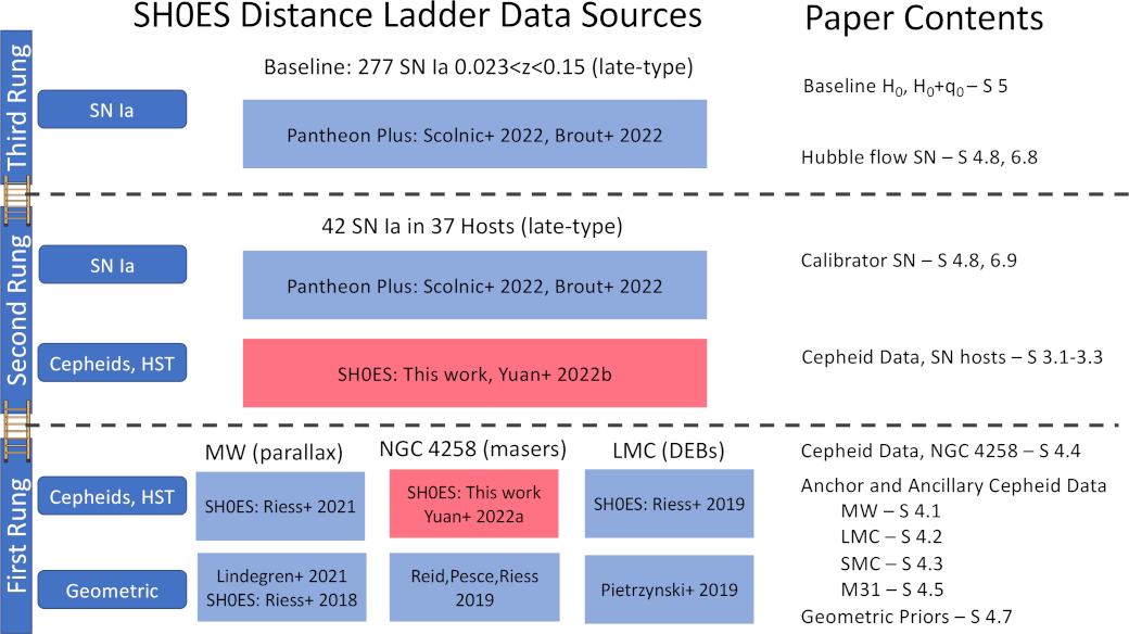
Figure 1: Sources of data for distance ladder. Red block shows data from this work.

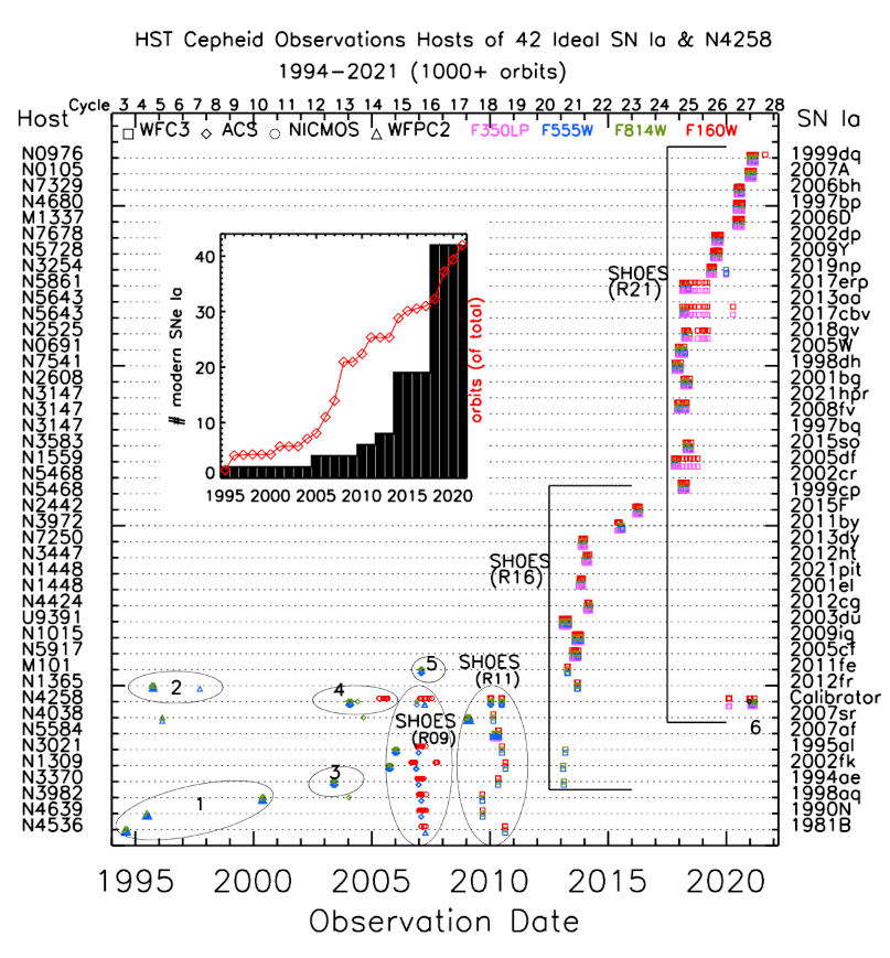
Figure 2: HST observations of Cepheids in 37 hosts of 42 “ideal” SNe Ia and NGC 4258, collected over 20 yr with 4 cameras and $>1000$ orbits of HST time. In most cases, 60 to 90-day campaigns in F555W and F814W or in F350LP were used to identify Cepheids from their light curves with occasional observations years later to identify longer-period Cepheids. NIR follow-up observations in F160W are used to reduce the effects of host-galaxy extinction, sensitivity to metallicity, and breaks in the $P$–$L$ relation. Data sources: (1) HST Key Project, freedman01; (2) HST SN Ia Luminosity Calibration Program, sandage06; (3) riess05; (4) macri06; (5) Mager:2013; (6) Yuan:2021_N4258.

Unlike the first-generation programs, which were granted long-term status and a large initial allocation of observing time with HST, the SH0ES program was proposed to the STScI time-allocation committee year-by-year. The cumulative result, after fifteen years (cycles), has been to collect Cepheid observations in 37 hosts of 42 SNe Ia and calibrate them geometrically to Cepheids in the MW, the LMC, and NGC 4258, with a total of 18 individual HST proposals utilizing $>1000$ orbits. The source of the distance-ladder data is shown in Fig. 1 and the source and sequence of all observations in SN Ia hosts are shown in Fig. 2 and listed in Table 1. Observing Cepheids in hosts at $D\approx 40$–50 Mpc, double the range of first-generation observations and a factor of 8 increase in targets, was feasible owing to two features of WFC3: significantly better sampling of the point-spread function (PSF), with pixel sizes a factor of 2.5 smaller than the wide channel of WFPC2 which greatly reduced the impact of crowded backgrounds, and a white-light filter (F350LP) that, combined with the better sensitivity of WFC3, reduced the observing time required to identify Cepheids and measure their periods by a factor of $\sim 4$. Calibrating those Cepheids differentially to bright Cepheids in the MW and LMC became feasible through the development of spatial scanning of HST and a rapid slew and guiding mode under gyroscopic control.

Table 1: Cepheid Observations with HST

		Exposure time [s]
Galaxy	SN(e) Ia	WFC3		All	NIR	UT
		NIRa	UVISb	opt.c	Prop ID(s)	Dated
M101	2011fe	4846	3776	53072	12880	2013-03-03
Mrk1337	2006D	13823	25994	25994	15640	2020-04-15
N0105	2007A	13270	34302	34302	16269	2020-10-23
N0691	2005W	9647	31413	31413	15145	2017-11-10
N0976	1999dq	15482	34312	34312	16269	2020-11-21
N1015	2009ig	14364	39336	39336	12880	2013-06-30
N1309	2002fk	6991	30020	89282	11570,12880	2010-07-24
N1365	2012fr	3617	31800	91200	12880	2013-08-06
N1448	2001el,2021pit	6035	17562	17562	12880	2013-09-15
N1559	2005df	10058	22245	22245	15145	2017-09-09
N2442	2015F	6035	20976	20976	13646	2016-01-21
N2525	2018gv	9821	21177	21177	15145	2018-02-14
N2608	2001bg	9647	26942	26942	15145	2018-02-04
N3021	1995al	4426	29620	88722	11570,12880	2010-06-03
N3147	1997bq,2008fv,2021hpr	14470	37426	37426	15145	2017-10-28
N3254	2019np	8441	22106	22106	15640	2019-03-11
N3370	1994ae	4376	29820	88222	11570,12880	2010-04-04
N3447	2012ht	4529	19114	19114	12880	2013-12-15
N3583	2015so	9647	27001	27001	15145	2018-03-06
N3972	2011by	6635	19932	19932	13647	2015-04-19
N3982	1998aq	4017	14000	90840	11570	2009-08-04
N4038	2007sr	6794	20640	85684	11577	2010-01-22
N4258	Anchor	40234	10120	103690	11570	2020-01-02
N4424	2012cg	3623	17782	17782	12880	2014-01-08
N4536	1981B	2564	26000	95000	11570	2010-07-19
N4639	1990N	5379	16000	77480	11570	2009-08-07
N4680	1997bp	9647	25217	25217	15640	2020-04-24
N5468	1999cp,2002cr	14470	36566	36566	15145	2017-12-22
N5584	2007af	4929	74940	74940	11570	2010-04-04
N5643	2013aa,2017cbv	9052	24741	24741	15145	2018-01-16
N5728	2009Y	13823	26111	26111	15640	2019-05-05
N5861	2017erp	10058	21798	21798	15145	2018-01-13
N5917	2005cf	7235	23469	23469	12880	2013-05-20
N7250	2013dy	5435	18158	18158	12880	2013-11-08
N7329	2006bh	9044	24665	24665	15640	2020-05-06
N7541	1998dh	9647	26766	26766	15145	2017-09-21
N7678	2002dp	12058	32060	32060	15640	2019-05-25
U9391	2003du	13711	39336	39336	12880	2012-12-14

Note. — (a) Obtained with WFC3/NIR and F160W; (b) obtained with WFC3/UVIS and F555W, F814W, or F350LP used to find and measure the flux of Cepheids; (c) includes time-series data from an earlier program and a different camera — see Fig. 2; (d) date of first WFC3/NIR observation;

The first SH0ES results (riess09a, hereafter R09) were based on Cepheids observed in the hosts of 6 ideal SN Ia calibrators using ACS (optical) and NICMOS (NIR), and one geometric anchor (NGC 4258) with a maser-based distance of 3% precision (Humphreys13) and a large sample of Cepheids (macri06). The result was a 5% measurement of H₀, $74.2\pm 3.6$ km s^-1 Mpc^-1, which combined with the 5-year WMAP results (Komatsu:2009) yielded $w=-1.12\pm 0.12$ and was consistent with a value of H${}_{0}=71.9\pm 2.6$ determined from WMAP and $\Lambda$CDM alone. The second iteration (riess11, hereafter R11) increased the calibrator sample to 8 SNe Ia, observed and measured all Cepheids with WFC3 (both optical and NIR), and expanded the geometric calibration of Cepheids beyond NGC 4258 by including two additional independent anchors: the LMC, through various DEB-based distances (e.g., Pietrzynski:2009), and the MW via parallaxes measured with the Fine Guidance Sensor on HST (benedict07). This resulted in H${}_{0}=73.8\pm 2.4$, which coupled with the 7-year WMAP results (komatsu11) yielded $w=-1.08\pm 0.10$, or an estimate of the effective number of relativistic species of $N_{\rm eff}=4.2\pm 0.7$. This result was closely matched by a recalibration of the final HST Key Project results using the same MW parallaxes, different Cepheid measurements, and an updated Hubble diagram of SNe Ia which yielded H${}_{0}=74.4\pm 2.2$ (freedman12, hereafter F12). Indications of any tension between the early and late Universe at that time were $<2\sigma$ in significance.

1.2 The Hubble Tension

The first release of CMB data from the ESA Planck mission (Planck:2013) yielded H${}_{0}=67.2\pm 1.2$ in the context of $\Lambda$CDM, a then $2\sigma$ reduction relative to WMAP and a difference of $3\sigma$ from the results of R11 and F12. Reanalyses of the R11 data (Fiorentino:2013; Efstathiou:2014; Zhang:2017) produced essentially the same results as R11, with H₀ ranging from 72.5 to 76.0. The third iteration of SH0ES (Riess:2016, hereafter R16) more than doubled the calibrator sample to 19 SNe Ia, used refined distance estimates to NGC 4258 and the LMC (Pietrzynski:2013), and new Cepheid parallaxes measured by the SH0ES team using spatial scanning with WFC3 (riess14; Casertano:2016) to reach a 2.4% determination of H${}_{0}=73.2\pm 1.7$, $3.4\sigma$ greater than the refined value from Planck$+\Lambda$CDM of $66.9\pm 0.6$ (Planck:2016), a difference of $\sim 9$% or 0.2 mag in units of 5 log H₀. An extensive number of reanalyses of the R16 data with many variations were undertaken (Cardona:2017; Feeney:2017; Follin:2017; Bovy:2018; Burns:2018; Dhawan:2018; Avelino:2019), resulting in H₀ values ranging from 73 to 74 and uncertainties from 2% to 2.5%. These analyses explored varying reddening laws, use of NIR SN data, use of alternative SN light-curve fitting, and hierarchical Bayesian statistics for data fitting, resulting in little change in H₀ or its uncertainty. Javanmardi:2021 selected the Cepheid host from R16 with the largest sample of Cepheids (NGC 5584, also near the median sample host distance) and remeasured these starting from the archived HST pixels and using different methods to do photometry, finding agreement with the R16 measurement to 1% precision and ruling out a significant methodological error in these measurements.

Since then, additional sources of MW parallax calibration of Cepheid luminosities have come from further use of HST WFC3 spatial scanning (Riess:2018a), from Gaia DR2 Cepheid parallaxes with HST photometry (Riess:2018b), from Gaia DR2 Cepheid binary companions and cluster hosts (Breuval:2020), and from Gaia EDR3 parallaxes coupled with additional HST photometry (Riess:2021). Likewise, HST observations of 70 long-period Cepheids in the LMC (Riess:2019) and improved distance estimates to the LMC (Pietrzynski:2019) and NGC 4258 (Reid:2019) resulted in H${}_{0}=73.2\pm 1.3$, raising the difference with Planck$+\Lambda$CDM to $4.2\sigma$. Other precise measures of H₀ in the local Universe from the distance–redshift relation generally range from 70 to 75, and those grounded in the pre-recombination version of $\Lambda$CDM range from 67 to 68, and have been extensively reviewed (Verde:2019; Divalentino:2021; Shah:2021). Because the tension is seen between different routes which are comparable only via an accurate cosmological model, numerous possible theoretical explanations for the emergent “Hubble tension” have been proposed but no consensus has yet emerged (Divalentino:2021). Indeed, theoretical priors weigh heavily on these proposals or whether it may be considered “extraordinary” for the $\Lambda$CDM model to fail or pass this cosmic test. The test itself, however, is empirical and few would conclude it has yet been satisfactorily passed.

1.3 This Work

In this publication, we more than double the sample of SN Ia calibrators from 19 in R16 to reach 42 objects in 37 hosts. This increase is a milestone for a sample whose size has limited the precision to which H₀ can be locally measured. It provides the largest increase in size we can anticipate in the remaining lifetime of HST as it now includes all suitable SNe Ia (of which we are aware) observed between 1980 and 2021 at $z<0.011$ and which slowly accrue at $\sim 1$ yr^-1. We have also reprocessed and reanalyzed the NIR observations of Cepheids in the previous 19 hosts reported by R16 for consistency with the new sample. We make use of an automated pipeline (Yuan:2021_SN, hereafter Y22b) to find the Cepheids in 18 new hosts (and reanalyze past hosts) which follow the steps developed manually for the first 19 hosts (Hoffmann:2016, hereafter H16). We benefit from a factor of 3 increase in the sample of Cepheids within NGC 4258 discovered by observing 4 new fields with HST, fully reanalyzed using the same pipeline by Yuan:2021_N4258. Extensive details concerning the analysis of SN Ia data are given by Scolnic:2021 and Brout:2022.

We present the formalism for measuring H₀ from the distance ladder in §2; new Cepheid data in §3 and in Y22a+Y22b; ancillary data used to measure H₀ in §4; our baseline, local determination of H₀ and a simultaneous measurement of H₀ and the expansion history with high-redshift SNe Ia in §5; extensions to the baseline and variants of the local measurement of H₀ in §6; discussion in §7; and conclusions in §8. Appendices provide further details on characterizing the spectral and photometric properties of the 42 calibrator SNe Ia (A), independent tests of the accuracy of Cepheid photometry (B), the Cepheid metallicity scale (LABEL:sc:appc), and alternative applications of “Wesenheit” magnitudes (LABEL:sc:appd).

2 Measuring the Hubble Constant

2.1 Distance-Ladder Formalism

The Hubble constant is the present relation between redshift and distance, $cz=$ H${}_{0}D$, measured at cosmological distances where expansion is the dominant source of redshift. Here it is measured via a three-step (or three-rung) distance ladder employing a single, simultaneous fit between (1) geometric distance measurements to standardized Cepheid variables, (2) standardized Cepheids and colocated SNe Ia in nearby galaxies, and (3) SNe Ia in the Hubble flow. The fit is accomplished simultaneously by optimizing a $\chi^{2}$ statistic to determine the most likely values of the parameters in the relevant relations. The data include measurements, their uncertainties, and their covariances as described in the next section. The parameters are the distances of all hosts and five additional parameters: the fiducial luminosity of SNe Ia and Cepheids, two parameters standardizing Cepheid luminosities (their dependence on period and metallicity), and H₀. This parameterization of the distance ladder can be expressed as a simple system of linear equations in a compact set of matrices as given below, useful for transmission, and for which the maximum-likelihood solution is easily found. The distance-ladder data and scheme are displayed in approximate form in Fig. 1.

To briefly summarize the relevant relations, the distance modulus of a source is $\mu_{0}=m_{0}-M_{0}=5\,{\rm log}\,D+25$, with $D$ the luminosity distance in Mpc, $m$ the apparent magnitude (flux), $M$ the absolute magnitude (luminosity), and the subscript 0 denoting a magnitude free of (or corrected for) intervening absorption by interstellar dust. The form of the dependence of Cepheid or SN Ia luminosity on observed characteristics (i.e., “standardization”) has been well-determined by prior work and is only briefly reviewed here. The dereddened Cepheid apparent magnitudes (also called “Wesenheit” magnitudes; madore82) at mean-phase will be described in §3.3 and are identified here as $m_{H}^{W}$ (in a specific host like NGC 4258, those Cepheids would have magnitudes given as $m^{W}_{H,N4258}$). For the $j$-th such Cepheid magnitude in the $i$-th host given the period $P_{i,j}$ in days and metallicity ${\rm[O/H]}_{i,j}$ relative to the Sun, we have

$$m_{H,i,j}^{W}=\mu_{0,i}+M_{H,1}^{W}+b_{W}\,(\log\,P_{i,j}-1)+Z_{W}{\rm[O/H]}_{i,j},$$ (1)

where $M_{H,1}^{W}$ is the fiducial absolute magnitude (in the Wesenheit magnitude system of 3.4), of a Cepheid with $\log\,P\!=\!1$ ($P\!=\!10$ days) and solar metallicity, and the parameters $b_{W}$ and $Z_{W}$ (sometimes called $\gamma$ in the literature) define the empirical relation between Cepheid period, metallicity, and luminosity. The ${\rm[O/H]}_{i,j}$ is inferred at its galactocentric radial position as described in §3.5.

Any number of Cepheid hosts may have an independent geometric distance which contributes to calibrating the Cepheid luminosity; e.g., for variables observed in the maser host NGC 4258 we adopt a distance modulus $\mu_{0,\rm N4258}$, the best estimate of the distance, with formal uncertainty $\sigma(\mu_{0,{\rm N4258}})$ from Reid:2019. In this case the individual host distance parameter $\mu_{0,i}$ above is replaced with the external constraint, converting the apparent magnitudes to absolute,

$$M_{H,j}^{W}=m_{H,N4258,j}^{W}\!-\!\mu_{0,\rm N4258}+\Delta\mu_{\rm N4258},$$ (2)

and introducing a new parameter $\Delta\mu_{\rm N4258}$ as the difference from the measured and true distance with the additional, simultaneous constraint equation $0=\Delta\mu_{\rm N4258}\pm\sigma(\mu_{0,{\rm N4258}})$. This definition allows the simultaneous use of multiple geometric “anchors” to calibrate the distance ladder; as we later show, it also allows the use of additional distance indicators for the same anchor, such as the tip of the red giant branch (TRGB) or Mira variable stars, while keeping track of their mutual dependence on the same geometric constraint.

A set of hosts of both SNe Ia and Cepheids connects the two distance indicators. Thus, for an SN Ia in the $i$-th Cepheid host,

$$m_{B,i}^{0}=\mu_{0,i}\!+\!M_{B}^{0},$$ (3)

where $m_{B,i}^{0}$ is its maximum-light apparent magnitude which has been standardized (i.e., corrected for variations around the fiducial color, luminosity, and any host dependence; see Scolnic:2021), $M_{B}^{0}$ is the fiducial SN Ia luminosity, and $\mu_{0,i}$ is the same parameter as in Equation (1). For SNe Ia, unlike Cepheids, the convention for keeping track of covariance in the standardization, as described by Scolnic:2021, is to employ a set of standardized $m_{B,i}^{0}$, their uncertainties, and the covariance between any pair. This is an equally mathematically valid approach as keeping track of covariance through the standardizing relation for Cepheids in Equation (1).

The ladder is completed with a set of SNe Ia that measure the expansion rate quantified as the intercept, $a_{B}$, of the distance (or magnitude)–redshift relation. This is simply $a_{B}=\log\,cz-0.2m_{B}^{0}$ in the low-redshift limit ($z\approx 0$) but given for an arbitrary expansion history and for $z>0$ as

$$a_{B}=\log\,cz\left\{1+{\frac{1}{2}}\left[1-q_{0}\right]{z}-{\frac{1}{6}}\left[1-q_{0}-3q_{0}^{2}+j_{0}\right]z^{2}+O(z^{3})\right\}-0.2m_{B}^{0},$$ (4)

measured from a set of SNe Ia ($z,m_{B}^{0}$) where $z$ is the redshift due to expansion, $q_{0}$ is the deceleration parameter, and $j_{0}$ is the jerk (see Visser:2004, for definitions). The determination of H₀ follows from

$$\log\,{\rm H}_{0}={0.2M_{B}^{0}\!+\!a_{B}\!+\!5}.$$ (5)

If the set of standardized SN Ia magnitudes in the hosts of Cepheids which serve to calibrate $M_{B}^{0}$ (hereafter “calibrators” or CC SNe Ia) and those in the Hubble flow used to measure $a_{B}$ (hereafter HF SNe Ia) have no common sources of uncertainty (i.e., no covariance), then Equations (3) and (4) and the ladder parameters they provide ($M_{B}^{0}$ and $a_{B}$) can be determined independently. This was the approach taken by R16. However, an increasingly thorough quantification of systematic uncertainties in SN Ia measurements, and the standardization undertaken as common practice for the determination of $w$ (Scolnic:2018), have demonstrated nontrivial covariance of SN Ia data, quantified following the approach of Conley:2011 and Dhawan:2020. We therefore undertake the optimization of Equations (3) and (5) simultaneously.

It is useful to expand the same set of Equations (1)–(5) in the form of matrices that organize the data into a vector of magnitude measurements ${\bf y}$, covariance matrix of standard errors of the magnitude measurements ${\bf C}$, equation matrix ${\bf L}$, and vector of free parameters ${\bf q}$ (hence the model, ${\bf Lq}$) as follows:

$$y=\begin{array}[]{ll}\left(\begin{array}[c]{c}m^{W}_{H,1}\\ ..\!\!\\ m^{W}_{H,\textrm{nh}}\\ \hline\cr m^{W}_{H,\textrm{N4258}}-\mu_{0,\textrm{N4258}}\\ m^{W}_{H,\textrm{M31}}\\ m^{W}_{H,\textrm{LMC}}-\mu_{0,\textrm{LMC}}\\ \hline\cr m_{B,1}^{0}\\ ..\!\!\\ m_{B,\textrm{ncc}}^{0}\\ \hline\cr M_{H,1,\textit{HST}}^{W}\\ M_{H,1,{\textit{G}aia}}^{W}\\ 0\\ 0\\ 0\\ \hline\cr m_{B,1}^{0}-5\log cz_{1}\{\}-25\\ ..\!\!\\ m_{B,\textrm{nhf}}-5\log cz_{\textrm{nhf}}\{\}-25\end{array}\right)&\begin{array}[c]{@{}l@{\,}l}\left.\begin{array}[]{c}\vphantom{m^{W}_{H,\textrm{nh},j}}\\ \vphantom{..\!\!}\\ \vphantom{\textrm{\LARGE HELLO}}\end{array}\right\}&\text{Cepheids in SN Ia hosts}\\ \left.\begin{array}[]{c}\vphantom{m^{W}_{H,\textrm{nh},j}}\\ \vphantom{m^{W}_{H,\textrm{nh},j}}\\ \vphantom{\textrm{\LARGE HELLO}}\end{array}\right\}&\text{Cepheids in anchors or non-SN~{}Ia hosts\hskip 108.405pt}\\ \left.\begin{array}[]{c}\vphantom{m^{W}_{H,\textrm{nh},j}}\\ \vphantom{..\!\!}\\ \vphantom{\textrm{\LARGE HELLO}}\end{array}\right\}&\text{SNe~{}Ia in Cepheid hosts}\\ \left.\begin{array}[]{c}\vphantom{m^{W}_{H,\textrm{nh},j}}\\ \vphantom{\textrm{\LARGE HELLO}}\\ \vphantom{0}\\ \vphantom{m^{W}_{H,\textrm{nh},j}}\\ \vphantom{\textrm{\LARGE HELLO}}\end{array}\right\}&\text{External constraints}\\ \left.\begin{array}[]{c}\vphantom{m^{W}_{H,\textrm{nh},j}}\\ \vphantom{..\!\!}\\ \vphantom{\textrm{\LARGE HELLO}}\end{array}\right\}&\text{SNe~{}Ia in the Hubble flow}\\ \end{array}\end{array}$$

$$C=\setcounter{MaxMatrixCols}{17}\begin{pmatrix}\scriptstyle{\sigma_{{\rm tot},1}^{2}}\!\!\!\!&..\!\!&Z_{\textrm{cov}}&Z_{\textrm{cov}}&\scriptstyle{0}&\scriptstyle{0}&\scriptstyle{0}&..\!\!&\scriptstyle{0}&\scriptstyle{0}&\scriptstyle{0}&\scriptstyle{0}&\scriptstyle{0}&\scriptstyle{0}&\scriptstyle{0}&..\!\!&\scriptstyle{0}\\ ..\!\!&..\!\!&..\!\!&..\!\!&..\!\!&..\!\!&..\!\!&..\!\!&..\!\!&..\!\!&..\!\!&..\!\!&..\!\!&..\!\!&..\!\!&..\!\!&..\!\!\\ Z_{\textrm{cov}}&..\!\!&\scriptstyle{\sigma_{{\rm tot},{\rm nh}}^{2}}\!\!\!\!&Z_{\textrm{cov}}&\scriptstyle{0}&\scriptstyle{0}&\scriptstyle{0}&..\!\!&\scriptstyle{0}&\scriptstyle{0}&\scriptstyle{0}&\scriptstyle{0}&\scriptstyle{0}&\scriptstyle{0}&\scriptstyle{0}&..\!\!&\scriptstyle{0}\\ \hline\cr Z_{\textrm{cov}}&..\!\!&Z_{\textrm{cov}}&\scriptstyle{\sigma_{{\rm tot},{\rm N4258}}^{2}}\!\!\!\!&\scriptstyle{0}&\scriptstyle{0}&\scriptstyle{0}&..\!\!&\scriptstyle{0}&\scriptstyle{0}&\scriptstyle{0}&\scriptstyle{0}&\scriptstyle{0}&\scriptstyle{0}&\scriptstyle{0}&..\!\!&\scriptstyle{0}\\ \scriptstyle{0}&..\!\!&\scriptstyle{0}&\scriptstyle{0}&\scriptstyle{\sigma_{{\rm tot},{\rm M31}}^{2}}\!\!\!\!&\scriptstyle{0}&\scriptstyle{0}&..\!\!&\scriptstyle{0}&\scriptstyle{0}&\scriptstyle{0}&\scriptstyle{0}&\scriptstyle{0}&\scriptstyle{0}&\scriptstyle{0}&..\!\!&\scriptstyle{0}\\ \scriptstyle{0}&..\!\!&\scriptstyle{0}&\scriptstyle{0}&\scriptstyle{0}&\scriptstyle{\sigma_{{\rm tot},{\rm LMC}}^{2}}\!\!\!\!&\scriptstyle{0}&..\!\!&\scriptstyle{0}&\scriptstyle{0}&\scriptstyle{0}&\scriptstyle{0}&\scriptstyle{0}&\scriptstyle{0}&\scriptstyle{0}&..\!\!&\scriptstyle{0}\\ \hline\cr\scriptstyle{0}&..\!\!&\scriptstyle{0}&\scriptstyle{0}&\scriptstyle{0}&\scriptstyle{0}&\scriptstyle{\sigma^{2}_{m_{\textsc{b}},1}}\!\!\!\!&..\!\!&{\rm SN}_{\textrm{cov}}&\scriptstyle{0}&\scriptstyle{0}&\scriptstyle{0}&\scriptstyle{0}&\scriptstyle{0}&{\rm SN}_{\textrm{cov}}&..\!\!&{\rm SN}_{\textrm{cov}}\\ ..\!\!&..\!\!&..\!\!&..\!\!&..\!\!&..\!\!&..\!\!&..\!\!&..\!\!&..\!\!&..\!\!&..\!\!&..\!\!&..\!\!&..\!\!&..\!\!&..\!\!\\ \scriptstyle{0}&..\!\!&\scriptstyle{0}&\scriptstyle{0}&\scriptstyle{0}&\scriptstyle{0}&{\rm SN}_{\textrm{cov}}&..\!\!&\scriptstyle{\sigma^{2}_{m_{\textsc{b},\textrm{ncc}}}}\!\!\!\!&\scriptstyle{0}&\scriptstyle{0}&\scriptstyle{0}&\scriptstyle{0}&\scriptstyle{0}&{\rm SN}_{\textrm{cov}}&..\!\!&{\rm SN}_{\textrm{cov}}\\ \hline\cr\scriptstyle{0}&..\!\!&\scriptstyle{0}&\scriptstyle{0}&\scriptstyle{0}&\scriptstyle{0}&\scriptstyle{0}&..\!\!&\scriptstyle{0}&\scriptstyle{\sigma_{\it HST}^{2}}&\scriptstyle{0}\!\!\!\!&\scriptstyle{0}&\scriptstyle{0}&\scriptstyle{0}&\scriptstyle{0}&..\!\!&\scriptstyle{0}\\ \scriptstyle{0}&..\!\!&\scriptstyle{0}&\scriptstyle{0}&\scriptstyle{0}&\scriptstyle{0}&\scriptstyle{0}&..\!\!&\scriptstyle{0}&\scriptstyle{0}&\scriptstyle{\sigma_{\it Gaia}^{2}}&\scriptstyle{0}\!\!\!\!&\scriptstyle{0}&\scriptstyle{0}&\scriptstyle{0}&..\!\!&\scriptstyle{0}\\ \scriptstyle{0}&..\!\!&\scriptstyle{0}&\scriptstyle{0}&\scriptstyle{0}&\scriptstyle{0}&\scriptstyle{0}&..\!\!&\scriptstyle{0}&\scriptstyle{0}&\scriptstyle{0}&\scriptstyle{\sigma_{\rm grnd}^{2}}\!\!\!\!&\scriptstyle{0}&\scriptstyle{0}&\scriptstyle{0}&..\!\!&\scriptstyle{0}\\ \scriptstyle{0}&..\!\!&\scriptstyle{0}&\scriptstyle{0}&\scriptstyle{0}&\scriptstyle{0}&\scriptstyle{0}&..\!\!&\scriptstyle{0}&\scriptstyle{0}&\scriptstyle{0}&\scriptstyle{0}&\scriptstyle{\sigma_{\mu,{\rm N4258}}^{2}}\!\!\!\!&\scriptstyle{0}&\scriptstyle{0}&..\!\!&\scriptstyle{0}\\ \scriptstyle{0}&..\!\!&\scriptstyle{0}&\scriptstyle{0}&\scriptstyle{0}&\scriptstyle{0}&\scriptstyle{0}&..\!\!&\scriptstyle{0}&\scriptstyle{0}&\scriptstyle{0}&\scriptstyle{0}&\scriptstyle{0}&\scriptstyle{\sigma_{\mu,{\rm LMC}}^{2}}&\scriptstyle{0}&..\!\!&\scriptstyle{0}\\ \hline\cr\scriptstyle{0}&..\!\!&\scriptstyle{0}&\scriptstyle{0}&\scriptstyle{0}&\scriptstyle{0}&{\rm SN}_{\textrm{cov}}&..\!\!&{\rm SN}_{\textrm{cov}}&\scriptstyle{0}&\scriptstyle{0}&\scriptstyle{0}&\scriptstyle{0}&\scriptstyle{0}&\scriptstyle{\sigma^{2}_{m_{\textsc{b}},z,1}}\!\!\!\!&..\!\!&{\rm SN}_{\textrm{cov}}\\ ..\!\!&..\!\!&..\!\!&..\!\!&..\!\!&..\!\!&..\!\!&..\!\!&..\!\!&..\!\!&..\!\!&..\!\!&..\!\!&..\!\!&..\!\!&..\!\!&..\!\!\\ \scriptstyle{0}&..\!\!&\scriptstyle{0}&\scriptstyle{0}&\scriptstyle{0}&\scriptstyle{0}&{\rm SN}_{\textrm{cov}}&..\!\!&{\rm SN}_{\textrm{cov}}&\scriptstyle{0}&\scriptstyle{0}&\scriptstyle{0}&\scriptstyle{0}&\scriptstyle{0}&{\rm SN}_{\textrm{cov}}&..\!\!&\scriptstyle{\sigma^{2}_{m_{\textsc{b},z,\textrm{nhf}}}}\!,\end{pmatrix}$$

where $\sigma_{{\rm tot},1}^{2}$ representing the $n\times n$ covariance matrix for the Cepheids in the first host is expanded as

$$\sigma_{{\rm tot},j}^{2}=\!\begin{pmatrix}\scriptstyle{\sigma_{{\rm tot},1,1}^{2}}\!\!\!\!&..\!\!&C_{1,1,n,bkgd}\\ ..\!\!&..\!\!&..\!\!\\ C_{1,n,1,bkgd}&..\!\!&\scriptstyle{\sigma_{{\rm tot},1,n}^{2}}\\ \end{pmatrix};$$

$$L=\begin{array}[]{ll}\left(\begin{array}[c]{cccccccccccc}\scriptstyle{1}&..\!\!&\scriptstyle{0}&\scriptstyle{0}&\scriptstyle{1}&\scriptstyle{0}&\scriptstyle{0}&\log P_{N,1}-1&\scriptstyle{0}&{\rm[O/H]}_{N,1}&\scriptstyle{0}&\scriptstyle{0}\\ ..\!\!&..\!\!&..\!\!&..\!\!&..\!\!&..\!\!&..\!\!&..\!\!&..\!\!&..\!\!&..\!\!&\scriptstyle{0}\\ \scriptstyle{0}&..\!\!&\scriptstyle{1}&\scriptstyle{0}&\scriptstyle{1}&\scriptstyle{0}&\scriptstyle{0}&\log P_{N,nh}-1&\scriptstyle{0}&{\rm[O/H]}_{N,nh}&\scriptstyle{0}&\scriptstyle{0}\\ \hline\cr\scriptstyle{0}&..\!\!&\scriptstyle{0}&\scriptstyle{1}&\scriptstyle{1}&\scriptstyle{0}&\scriptstyle{0}&\log P_{\textrm{N4258}}-1&\scriptstyle{0}&{\rm[O/H]}_{\textrm{N4258}}&\scriptstyle{0}&\scriptstyle{0}\\ \scriptstyle{0}&..\!\!&\scriptstyle{0}&\scriptstyle{0}&\scriptstyle{1}&\scriptstyle{0}&\scriptstyle{1}&\log P_{\textrm{M31}}-1&\scriptstyle{0}&{\rm[O/H]}_{\textrm{M31}}&\scriptstyle{0}&\scriptstyle{0}\\ \scriptstyle{0}&..\!\!&\scriptstyle{0}&\scriptstyle{0}&\scriptstyle{1}&\scriptstyle{1}&\scriptstyle{0}&\log P_{\textrm{LMC}}-1&\scriptstyle{0}&{\rm[O/H]}_{\textrm{LMC}}&\scriptstyle{1}&\scriptstyle{0}\\ \hline\cr\scriptstyle{1}&..\!\!&\scriptstyle{0}&\scriptstyle{0}&\scriptstyle{0}&\scriptstyle{0}&\scriptstyle{0}&\scriptstyle{0}&\scriptstyle{1}&\scriptstyle{0}&\scriptstyle{0}&\scriptstyle{0}\\ ..\!\!&..\!\!&..\!\!&..\!\!&..\!\!&..\!\!&..\!\!&..\!\!&..\!\!&..\!\!&..\!\!&\scriptstyle{0}\\ \scriptstyle{0}&..\!\!&\scriptstyle{1}&\scriptstyle{0}&\scriptstyle{0}&\scriptstyle{0}&\scriptstyle{0}&\scriptstyle{0}&\scriptstyle{1}&\scriptstyle{0}&\scriptstyle{0}&\scriptstyle{0}\\ \hline\cr\scriptstyle{0}&..\!\!&\scriptstyle{0}&\scriptstyle{0}&\scriptstyle{1}&\scriptstyle{0}&\scriptstyle{0}&\scriptstyle{0}&\scriptstyle{0}&\scriptstyle{0}&\scriptstyle{0}&\scriptstyle{0}\\ \scriptstyle{0}&..\!\!&\scriptstyle{0}&\scriptstyle{0}&\scriptstyle{1}&\scriptstyle{0}&\scriptstyle{0}&\scriptstyle{0}&\scriptstyle{0}&\scriptstyle{0}&\scriptstyle{0}&\scriptstyle{0}\\ \scriptstyle{0}&..\!\!&\scriptstyle{0}&\scriptstyle{0}&\scriptstyle{0}&\scriptstyle{0}&\scriptstyle{0}&\scriptstyle{0}&\scriptstyle{0}&\scriptstyle{0}&\scriptstyle{1}&\scriptstyle{0}\\ \scriptstyle{0}&..\!\!&\scriptstyle{0}&\scriptstyle{1}&\scriptstyle{0}&\scriptstyle{0}&\scriptstyle{0}&\scriptstyle{0}&\scriptstyle{0}&\scriptstyle{0}&\scriptstyle{0}&\scriptstyle{0}\\ \scriptstyle{0}&..\!\!&\scriptstyle{0}&\scriptstyle{0}&\scriptstyle{0}&\scriptstyle{1}&\scriptstyle{0}&\scriptstyle{0}&\scriptstyle{0}&\scriptstyle{0}&\scriptstyle{0}&\scriptstyle{0}\\ \hline\cr\scriptstyle{0}&..\!\!&\scriptstyle{0}&\scriptstyle{0}&\scriptstyle{0}&\scriptstyle{0}&\scriptstyle{0}&\scriptstyle{0}&\scriptstyle{1}&\scriptstyle{0}&\scriptstyle{0}&\scriptstyle{-1}\\ ..\!\!&..\!\!&..\!\!&..\!\!&..\!\!&..\!\!&..\!\!&..\!\!&..\!\!&..\!\!&..\!\!&..\!\!\\ \scriptstyle{0}&..\!\!&\scriptstyle{0}&\scriptstyle{0}&\scriptstyle{0}&\scriptstyle{0}&\scriptstyle{0}&\scriptstyle{0}&\scriptstyle{1}&\scriptstyle{0}&\scriptstyle{0}&\scriptstyle{-1}\\ \end{array}\right)\par&\begin{array}[c]{@{}l@{\,}l}\left.\begin{array}[]{c}\vphantom{\log P^{l}_{N}}\\ \vphantom{\log P^{l}_{N}}\\ \vphantom{\textrm{\LARGE HELLO}}\end{array}\right\}&\text{Cepheids in SN~{}Ia hosts}\\ \left.\begin{array}[]{c}\vphantom{\log P^{l}_{N}}\\ \vphantom{\log P^{l}_{N}}\\ \vphantom{\textrm{\LARGE HELLO}}\end{array}\right\}&\text{Cepheids in anchors or non-SN~{}Ia hosts\hskip 20.2355pt}\\ \left.\begin{array}[]{c}\vphantom{\log P^{l}_{N}}\\ \vphantom{\log P^{l}_{N}}\\ \vphantom{\textrm{\LARGE HELLO}}\end{array}\right\}&\text{SNe~{}Ia in Cepheid hosts}\\ \left.\begin{array}[]{c}\vphantom{\log P^{l}_{N}}\\ \vphantom{\log P^{l}_{N}}\\ \vphantom{\log P^{l}_{N}}\\ \vphantom{\log P^{l}_{N}}\\ \vphantom{\textrm{\LARGE HELLO}}\end{array}\right\}&\text{External constraints}\\ \left.\begin{array}[]{c}\vphantom{\log P^{l}_{N}}\\ \vphantom{\log P^{l}_{N}}\\ \vphantom{\textrm{\LARGE HELLO}}\end{array}\right\}&\text{SNe~{}Ia in the Hubble flow}\\ \end{array}\end{array}$$

$$q=\begin{pmatrix}\mu_{0,1}\\ ..\!\!\\ \mu_{0,\textrm{nh}}\\ \Delta\mu_{\rm N4258}\\ M_{H,1}^{W}\!\\ \Delta\mu_{\rm LMC}\\ \mu_{M31}\\ b_{W}\\ M_{B}^{0}\!\\ Z_{W}\\ \Delta{\rm zp}\\ 5\,\log\,\textrm{H}_{0}\end{pmatrix}.$$

The number of Cepheid hosts is nh, the number of SNe Ia in these hosts is ncc, and the number of SNe Ia in the Hubble flow is nhf. Period uncertainties are comparatively negligible (Yuan:2021_N4051). $\sigma_{\it HST},\ \sigma_{\it Gaia}$ denote the uncertainties in $M_{H,1,Gaia}^{W}$ and $M_{H,1,HST}^{W}$ as derived from parallaxes, respectively, while $\sigma_{\it grnd}$ denotes the uncertainty in ground-based photometry. The term ${\rm SN}_{\textrm{cov}}$ is the covariance between SNe, $Z_{\textrm{cov}}$ is the metallicity covariance given later in Equation (9), and $C_{i,j,k,bkgd}$ is the background covariance given later in Equation (8). The $\chi^{2}$ statistic is given as

$$\chi^{2}=(y-Lq)^{T}C^{-1}(y-Lq)$$ (6)

and maximum-likelihood parameters are given as $q_{\textit{best}}=(L^{T}C^{-1}L)^{-1}L^{T}C^{-1}y$, while the standard errors and the covariance matrix of the parameters come from the matrix $cq=(L^{T}C^{-1}L)^{-1}$. The value of H₀ is derived from the final entry of ${\bf q}$, $5\,\log\,$H₀, and its error from the square root of the corner entry of ${\bf cq}$. This provides a compact form for storing and transmitting the full dataset used to determine H₀, to edit or augment it, and to enable others to determine its value. The above formalism is the same as used by R16 with the additions of SN and Cepheid covariance. We will also derive the parameters independently of the analytical solution in §5.1 by sampling the $\chi^{2}$ statistic using a Markov Chain Monte Carlo (MCMC) approach to verify the analytical result with a different methodology.

3 Cepheid Observations in SN Ia Hosts and the Maser Host NGC 4258

3.1 Optical Cepheid Discovery

The SH0ES program has been selecting the SNe Ia that are most suitable for calibrating their fiducial luminosity (with selection criteria given in §1.1) through observations of Cepheids in their hosts. The results here include a complete sample of all such SNe Ia of which we are aware within $z<0.011$ (40 objects), with the addition of two beyond this limit that are useful for testing the range of Cepheid distance measurements, for a total of 42 SN Ia calibrators.

Fig. 2 and Table 1 show the sources of the HST data obtained for every SN Ia and host we measured, gathered from the indicated HST cameras, filters, and time periods. All of these publicly available data are readily obtained from the Mikulski Archive for Space Telescopes (MAST). The imaging data are used for both Cepheid discovery and their flux measurement. For the former, a campaign using a filter with central wavelength in the visual band and $\sim 11$–12 epochs with nonredundant spacings spanning $\sim 60$–100 days is optimal to identify Cepheid variables by their unique light curves and large amplitudes ($\sim 1$ mag peak-to-trough), and accurately measure their periods (madore91; saha96; Stetson:1996). Image subtraction may find additional Cepheids (Bonanos:2003), but these objects will be subject to greater photometric biases owing to blends which suppress their amplitudes and chances of discovery in time-series data (Ferrarese:2000). The data were collected from $\sim 150$ HST orbits with WFC3-NIR and $\sim 700$ orbits obtained for the optical identification (350 from WFC3, 170 from ACS, and 180 from WFPC2), including $\sim 200$ orbits from NICMOS superseded by WFC3-NIR, for a total of $\sim 1050$ HST orbits. Additional observations of Cepheids in the MW and LMC anchors utilized $\sim 200$ orbits or snapshots.

Earlier efforts contribute $\sim 200$ orbits of imaging of these hosts: 35 orbits from the HST Key Project, 105 from the SNe Ia Luminosity Program, 36 from Mager:2013, and 50 from macri06, with the remaining $\sim 800$ from SH0ES.

The procedure for identifying Cepheids from time-series optical data in visual or white light bands has been described extensively (saha96; Stetson:1996; riess05; macri06; Hoffmann:2016); details of the procedures followed for this sample are presented by Yuan:2021_SN. These procedures utilize the DAO suite of software tools (Stetson:1987; Stetson:1994) for crowded-field PSF photometry, and are similar to those used previously by the SH0ES team (Hoffmann:2016) and to a large extent by the first generation of HST-based H₀ measurements. Past work has demonstrated that the use of different photometry algorithms yields a largely overlapping list of Cepheids with similar periods and photometry (Ferrarese:1998).

The end result is a set of high-confidence Cepheids which have passed selection and quality cuts described by Y22b, with periods and mean colors (F555W–F814W) measured in the HST WFC3 photometric system. For each Cepheid, we estimate a precise position in the WFC3/NIR F160W images using a geometric transformation derived from the optical images using bright and isolated stars, with resulting mean position uncertainties for the variables $<0.03$ pix. The positions of the Cepheids are indicated in Fig. 3.

We present composite light curves of all Cepheids with $10<P<80$ d in Fig. 5 based on $\sim 60,000$ individual F555W or F350LP photometric measurements, which identify these as bona-fide classical Cepheids with the characteristic sawtooth light-curve shape of fundamental-mode pulsators. There are more subtle Cepheid light-curve features which are not apparent in individual examples at these distances. However, we can leverage the statistical power of the sample to look for these features as a strong validation test of the universality of Cepheids, as presented below.

3.2 Cepheid Validation: The Hertzsprung Progression

The shapes of Cepheid light curves change in subtle but characteristic ways (often referred to as the “Hertzsprung Progression”; Hertzsprung:1926) as a function of period, visible only with high signal-to-noise-ratio (SNR) observations. Hertzsprung:1926 noted the characteristic “quick rise and slow decrease” for most periods but also a small range of periods (9–13 d) where the light curves are quite symmetric, and the presence of a “bump” or small local maximum whose phase occurs earlier with increasing period, appearing on the descending phase at $P\approx 6$ d, merging with the main peak at $P\approx 10$ d, and appearing on the rising phase at $P\approx 10$–15 d before disappearing (variables where the bump is apparent are sometimes referred to as “bump” Cepheids). While the general fast rise and slow decline is a characteristic of a star pulsating in the fundamental mode, the “bump” is understood through modeling to arise from a 2:1 resonance between the fundamental and second overtone (Cox:1993; Bono:2002) and is a unique feature of classical Cepheids. Cepheids with $P>40$ d occur at the high-mass end of the luminosity function and are thus rare, with the MW hosting only a few examples which show a broadening of the light curve and a decrease in amplitude.

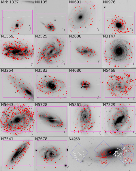
Figure 3: Images of 18 newly-observed hosts of 23 SNe Ia and NGC 4258. Each image is of the Cepheid host indicated. The magenta outline shows the $2.7^{\prime}\times 2.7^{\prime}$ field of the WFC3/NIR observations. Red dots indicate the positions of the Cepheids. Compass indicates north (long axis) and east (short axis). The NGC 4258 image shows Cepheids from macri06 in white and new ones from Yuan:2021_N4258 in red.

Figure 4: Pseudocolor images of all Cepheid-bearing galaxies analyzed in this work. From top left, 37 hosts of 42 SNe Ia presented in the same order as Table 1. The last row includes our three anchors (NGC 4258, MW, LMC) and two supporting galaxies (SMC, M31). Galaxies are presented at arbitrary plate scales, though in most cases the panels encompass the entire ACS or WFC3/UVIS field of view. Credits: SN hosts and NGC 4258 – ESA Hubble site; MW, LMC, and SMC – ESA Gaia site; M31 – STScI.

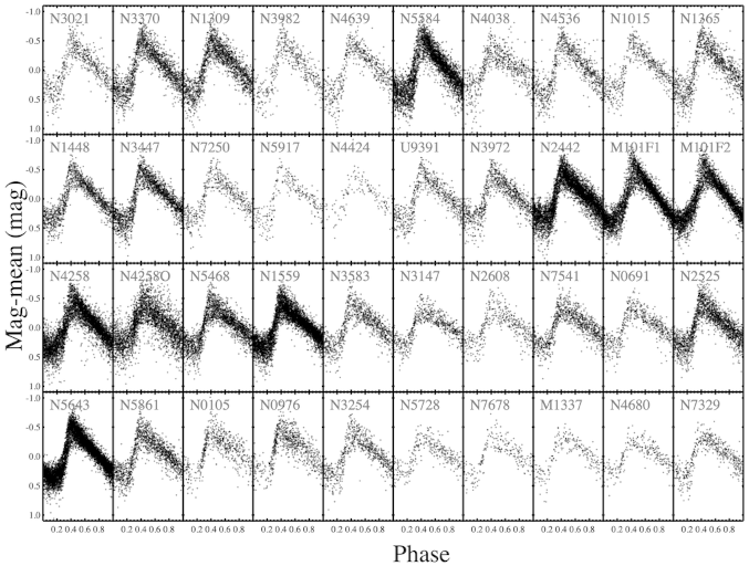
Figure 5: Composite visual ($F555W$) or white-light ($F350LP$) Cepheid light curves. Each HST Cepheid light curve with $10<P<80$ d is plotted after subtracting the mean magnitude and determining the phase of the observation.

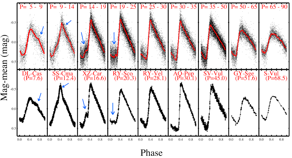
Figure 6: Composite visual ($F555W$) or white-light ($F350LP$) Cepheid light curves binned by period (upper) and compared with individual MW Cepheids near the middle period of the bin. The “Hertzsprung Progression” (relation between light-curve shape and period) is apparent, including subtle features like the progression in phase of a resonance “bump” between the second overtone and fundamental pulsation for $P<20$ d. The red line is a cubic spline constrained by the averages of bins in phase.

By binning all of the extragalactic light curves for the 37 SN Ia hosts and NGC 4258 by period as shown in Fig. 6, a striking display of this more subtle light-curve structure emerges. The resonance-induced bump is indicated on the descending phase at $P=5$–9 d with the MW Cepheid DL Cas ($P=7.6$ d) shown for comparison, the narrow-peaked, symmetric curve at $P=9$–14 d as in SS CMa ($P=12.4$ d), the resonance bump on the rising phase in the $P=14$–19 d as in XZ Car ($P=16.6$ d), before transitioning to sawtoothed curves in the next 3 bins ($P=19-35$ d). Beyond this range, we see the gradual transition to flatter and more sinusoidal curves matching the MW sequence of SV Vul ($P=45$ d), GY Sge ($P=52$ d), and S Vul ($P=69$ d).

While our pipeline selection requires candidate Cepheids to have amplitudes in the characteristic range of 0.2–1 mag, we impose no requirement regarding the presence of these more subtle light-curve features, which are not detectable at the data quality typical of single extragalactic Cepheids (Hoffmann:2016). The presence of these features in aggregate light curves at the appropriate periods offers an additional level of scrutiny and validation of these sources as classical Cepheids, as well as the means for a more detailed comparison to those in the MW. The impressive similarity of these light-curve sequences demonstrates the universality of the physics producing these pulsating standard candles, and provides an important test of their consistency along the distance ladder. The appearance of the Hertzsprung Progression among the extragalactic sample demonstrates these objects are bona-fide Cepheid variables.

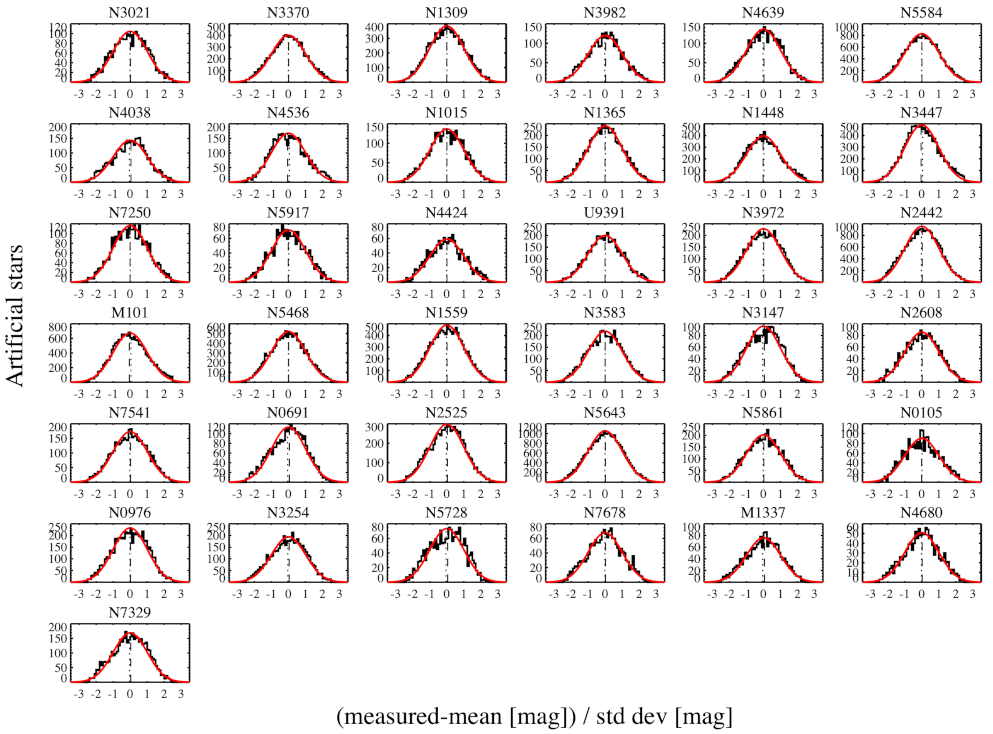
Figure 7: Distributions of recovered artificial stars in each host. For each real Cepheid, 100 artificial stars of the expected Cepheid magnitude (based on its period and the $P$–$L$ relation) are added to the host images within an annulus with an outer radius of $2.4^{\prime\prime}$ and measured following the same procedures as for the Cepheids to produce a distribution in magnitudes (log flux). The distributions for each host are combined after subtracting their mean and dividing by their standard deviation. They compare well to a Gaussian with a difference in median and mean (dashed and dotted lines) of $\sim 0.03\sigma$.

3.3 NIR Photometry and Validation in NGC 4258

Following the same procedures described by R16, we perform NIR photometry of the Cepheids using their positions derived and fixed from the higher-resolution optical data. The NIR images of all Cepheids were reprocessed for this analysis using revised calibrations by the STScI pipeline (including new flatfields and geometric-distortion tables), and we were able to predict the expected NIR positions of the Cepheids found in the optical data with enhanced precision compared to our previous reduction (Hoffmann:2016). Additional sources found in the NIR images are fit simultaneously with the Cepheids using an empirical model of the PSF derived from the solar-analogue star P330E. The background calibration and photometric uncertainties are determined from retrieval of 100 locally-placed artificial stars per Cepheid as described by R11 and R16.

In Fig. 7 we show the distributions of the artificial-star measurements divided by their standard deviation, which demonstrates that they are well approximated by Gaussian distributions in magnitude space around their mean out to $3\sigma$, a consequence of the log-normal distribution of underlying surface brightness fluctuations (primarily red giants, with larger and brighter collections increasingly rare) in the NIR. The mean difference between the mean and median of the artificial-star distributions, which vanishes for a true Gaussian, is $0.03\sigma$. Averaged across all SN hosts, the difference between mean and median of the magnitude distribution drops to $0.01\sigma$ or 4 millimag, showing no apparent correlation between its third moment (skewness) and the host distance. The distribution for the geometric calibrator, NGC 4258, appears similar to that of the others, with a difference between mean and median of 0.01 mag. These measurements justify the use of Gaussian statistics in magnitude space in the calculations to follow.

The accuracy of the background estimates owes to Cepheids being randomly superimposed on scenes, a consequence of our perspective whose local levels can be measured statistically. A caveat to this approach would be the presence of associated flux (colocated with the Cepheid) which becomes important only if it is then resolved for nearby Cepheids but not for distant ones. The level of such “associated flux” has been measured statistically from hundreds of Cepheids in M31 by Anderson:2018 to be $\sim 7$ millimag at distances beyond a few Mpc, and is due to associated open clusters that would not be resolved at those distances. This term is explicitly included here in the background estimates, in order to compensate for this effect. An additional and direct consequence of a potential miscalibration of the background, independent of Cepheid mean flux, would be a change in apparent light-curve amplitude. Riess:2020 determined that the NIR amplitudes of Cepheids in SN hosts are fully consistent with those in the Milky Way, yielding an independent upper limit of 0.03 mag for the possible misestimation of the background. The sensitivity of H₀ to the unresolved background can be further mitigated by the use of a distant anchor with similar background as the SN Ia hosts such as NGC 4258; this will be addressed in §4.

In Fig. 8 we provide a strong test of the background estimation by comparing the Cepheid photometry in dense (inner) and sparse (outer) regions of NGC 4258. Because the Cepheids in both fields are at the same distance from us and the metallicity gradient in NGC 4258 is small (Bresolin:2016), an apparent difference of the dereddened magnitudes would be a consequence of misestimating the background in the dense field. The difference in intercept (i.e., distance) is 0.01 mag and well within the indicated errors of the means, demonstrating that Cepheid PSF photometry is accurate in the presence of the same level of crowded backgrounds seen in the SN hosts..

In Appendix B we provide an independent validation of the PSF photometry using aperture photometry, a method which is accurate when the background is measured from the mean of pixels in concentric annuli and uncomplicated to apply, albeit less precise than the standard approach of using PSFs to model photometry. This test validates the mean PSF photometry in SN hosts to $\sigma\approx 0.02$ mag. In that Appendix we further perform an additional “null test” of the background estimates by regressing them against the distance ladder fit residuals, finding a dependence of $0.010\pm 0.014$ mag per magnitude of source background (in the sense of overestimating the background but with no significance).

In §7.1 we review multiple tests of Cepheid PSF photometry in addition to six strong tests of background estimates in the presence of crowded backgrounds, all of which indicate that the Cepheid measurements are accurate.

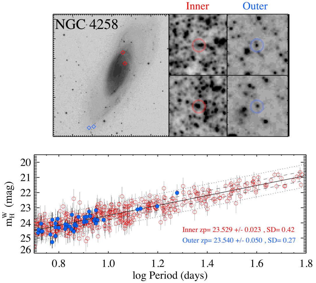
Figure 8: Comparison of Cepheids measured in a dense (inner) field (in red) and sparse (outer) field (in blue) of NGC 4258. Because these Cepheids are at the same distance, the comparison shows the accuracy of the background estimates which differ in the mean over the same sampled range, $0.7<\log(P/{\rm day})<1.2$, by 0.45 mag (relative to the Cepheids), yet yield a consistent intercept to $\sigma\approx 0.05$ mag. The difference in metallicity between the samples, $\Delta$[O/H] $=0.08$ dex, corresponds to a difference of 0.02 mag, smaller than the precision of this comparison.

3.4 Dereddened Magnitudes

The SH0ES program uses observations in HST filters at known Cepheid phases in optical (F555W, F814W) and NIR (F160W) bands to correct for the effects of interstellar dust and the finite width in temperature of the Cepheid instability strip. We employ NIR “Wesenheit” magnitudes (madore82) to deredden Cepheids throughout, defined as

$$m_{H}^{W}=m_{H}-R\,(m_{V}\!-\!m_{I}),$$ (7)

where $m_{H}=$ F160W, $m_{V}=$ F555W, and $m_{I}=$ F814W and $V-I=m_{V}-m_{I}$ in the HST system, and $R\equiv A_{H}/(A_{V}\!-\!A_{I})$. Wesenheit magnitudes are not conventional magnitudes, which compare the brightness of one star to another; rather, they are used to compare the brightness of one standardized candle to another through the removal of their unequal extinction, as reviewed in Appendix LABEL:sc:appd. While the value of $R$ obtained from well-characterized extinction laws for these bands is $\sim 0.4$, we note that the correlation between Cepheid intrinsic color and luminosity at a fixed period has the same sense as extinction (cooler is fainter), and is similar in size with an intrinsic value of $\sim 0.6$ (as discussed in §6.2). Therefore, the value of $R$ derived for extinction effectively also reduces the intrinsic scatter caused by the breadth of the instability strip. We analyze the sensitivity of H₀ to values of $R$ derived from different extinction laws in §6.3. In Appendix LABEL:sc:appd, we discuss pitfalls associated with varying $R$ in Equation (7) between galaxies if the intrinsic color is not first subtracted from the observed color (Follin:2017; Mortsell:2021).

To avoid a magnitude bias, we include only Cepheids with periods above the completeness limit of detection in our primary fit for each host (Y22b). The measurements of Cepheids in SN Ia hosts are provided in Table 2, while Table 3 summarizes the properties of the resulting NIR $P$–$L$ relations. We identify a number of improvements realized here since our previous Cepheid measurements in SN hosts $\sim 6$ yr ago (R16, H16), and $\sim 16$ yr ago for NGC 4258 (macri06).

Table 2: WFC3/NIR Cepheids

Field	$\alpha$	$\delta$	ID	$P$	Colora	$\sigma_{\rm col}$	F160W	$\sigma_{\rm tot}$	[O/H]	Note
	(J2000)			[d]	[mag]				[dex]
M101	210.91148	54.357230	54672	6.853	0.91	0.11	24.04	0.44	0.05	HST
M101	210.88464	54.338980	110830	6.873	1.05	0.19	23.36	0.62	0.09	HST

Note. — (a): F555W–F814W.

1. Sky annuli: The size of the annulus used to estimate the level of the sky value of the region around the Cepheid (after subtracting all detected sources) in $F160W$ was reduced in size to inner and outer radii of 0$\farcs$24 and 0$\farcs$8 (from 0$\farcs$96 and 1$\farcs$44 in R16) based on extensive simulations. This determination of the sky level is more precise, although it requires taking into account the contribution to the sky from the wings of the PSF; the resulting offset of 0.008 mag is robustly determined from bright stars and corrected in the final photometry. The random sky error is propagated to the photometry error through the sampling of sky values in the artificial-star analyses).

2. Determination of the background and covariance: As in R16, artificial stars are added in the F160W images in the vicinity of each Cepheid at the apparent magnitude expected from its period and trial fits of the $P$–$L$ relation. The difference between the input and recovered magnitudes is used to refine the initial estimate of the sky background and revise the Cepheid photometry. This process is necessarily iterative as the $P$–$L$ relation used to predict the magnitude of a given Cepheid from its period is determined after correcting the photometry based on the retrieval of the artificial stars. Thanks to greater processing power, we increased the number of iterations since R16, and found that in some cases the iterations in our previous work were not adequate (as they had not fully converged). The new process fully converges with improved determination of the trial intercepts and slopes, and we use the final iteration to estimate a systematic uncertainty of 20% of the background (in units of the Cepheid magnitude correction) as the covariance “error floor” of any pair of Cepheids, $j,k$ in the same $i$-th host, given by

   $$C_{i,j,k,{\rm bkgd}}=0.2^{2}(\textit{bkgd}_{i,j})(\textit{bkgd}_{i,k}).$$ (8)

   This provides a systematic uncertainty in the range of 0.03–0.06 mag for all Cepheids within each host, with the term bkgd representing the change in Cepheid magnitude due to the addition of the mean level of the crowded background from unresolved sources derived from the artificial stars. The artificial star magnitudes are determined from the trial P-L relations of each host independently from every other host so there is no source of background covariance between different hosts.

3. Reference Files: The photometry benefits from the latest STScI data pipelines, including new flatfields (with better “blob” mapping), bias frames, long-history dark frames, pixel-based CTE corrections for optical data, and geometric-distortion corrections, yielding improved alignment between the optical and NIR frames.

4. Count Rate Nonlinearity (CRNL): We adopt a new calibration of the WFC3/NIR CRNL (Riess:2019). By convention, this is applied to Cepheids in anchors between their flux and the background level of Cepheids in SN hosts.

5. M101 long-period Cepheids: A re-examination of the Cepheids in M101, together with simulations, revealed that the baseline of the original monitoring campaign (carried out in 2006 and reported by Mager:2013) was too short to provide reliable periods for apparent Cepheids with $P>35$ d (equivalent to $1.2\times$ the time span of the observations). Two additional epochs obtained 7 yr later and separated by a week are insufficient to resolve the issue, because at these periods the two epochs provide effectively only one phase measurement, and the prevailing period uncertainty of $>0.5$ d makes the phasing of the two sets unreliable. For that reason we exclude M101 Cepheids with $P>35$ d (about 10% of the sample used by R16).

6. We correct Cepheid periods to rest-frame values owing to $(1+z)$ time dilation (Anderson:2019), a small (given our typical $z\approx 0.005$) but one-sided effect.

We note that the Cepheid color measurements, $V\!-\!I$, employed in Eq. 7 to determine the baseline value of H₀ here and in R16 (as well as most variants) are relatively insensitive to the previously noted improvements to the calibration of the Cepheid optical measurements realized in the last 6 or 16 years and included in Y22a,b. These include the use of artificial stars to estimate the crowded backgrounds, revised flatfields, archival dark frames, updated geometric distortion maps to rectify frames, and pixel-based CTE corrections, most of which were not implemented by H16 or by macri06 from which the N 4258 data in H16 were derived.  These improvements cancel to first order in the difference, $V\!-\!I$, as do changes in CCD sensitivity which can decline on orbit or change abruptly when the electronics are refurbished as occurred for ACS in 2009.  However, the use of optical Wesenheit magnitudes to determine H₀ without bias (as we explore in §6.13) requires fully-calibrated optical magnitudes rather than only accurate optical colors (as in H16 and provided in R16). The fully-calibrated optical magnitudes available in Y22a,b are suitable for this purpose.

We do not attempt to quantify the impact of each of these improvements individually; however, in the aggregate, matching Cepheids within 1^′′ of those in R16, the net change to Cepheid photometry in F160W is that 63% (37%) of Cepheids are fainter (brighter). We provide additional details of this comparison in Appendix B.

Table 3: Properties of NIR $P$–$L$ Relations

Galaxy	Number			$\langle P\rangle$	$\langle$[O/H]$\rangle^{a}$
	FoV	meas.b	fitc	[day]	[dex]
M101	311	260	259	15.8	0.10
Mrk1337	21	20	15	52.9	-0.18
N0105	32	8	8	41.5	-0.13
N0691	31	28	28	46.5	0.09
N0976	57	35	33	40.2	0.02
N1015	26	20	18	52.5	-0.03
N1309	57	53	53	54.1	-0.08
N1365	66	47	45	29.0	-0.14
N1448	90	77	73	35.2	-0.11
N1559	136	110	110	34.4	0.00
N2442	238	177	177	36.0	0.00
N2525	85	73	73	40.4	0.10
N2608	25	22	22	45.4	0.11
N3021	26	16	16	32.2	0.06
N3147	29	28	27	52.3	0.17
N3254	54	48	48	41.5	-0.18
N3370	82	73	73	42.5	-0.12
N3447	116	102	101	36.0	-0.16
N3583	62	54	54	41.6	-0.06
N3972	66	54	52	32.3	0.03
N3982	31	27	27	29.9	-0.14
N4038	38	29	29	53.6	0.03
N4424	17	10	9	31.1	0.06
N4536	45	41	40	36.0	-0.15
N4639	36	30	30	38.7	-0.01
N4680	18	11	11	55.1	-0.06
N5468	118	93	93	54.9	-0.10
N5584	196	167	165	36.8	-0.10
N5643	294	251	251	31.8	0.13
N5728	25	20	20	44.3	0.15
N5861	60	41	41	43.8	0.06
N5917	17	14	14	37.9	-0.30
N7250	30	21	21	37.3	-0.28
N7329	38	31	31	54.6	0.17
N7541	50	33	33	49.1	-0.12
N7678	21	16	16	42.8	0.02
U9391	36	33	33	39.6	-0.22
SN Total	2680	2173	2150	36.5	-0.01
N4258	555	451	443	14.4	-0.10
M31	–	55	55	19.1	-0.11
LMCd	–	342	339	13.3	-0.29
SMC	–	145	143	13.3	-0.72
Total All	—	3165	3129	–	–

Note. — (a) Solar value: 12 + log [O/H] $=8.69$, asplund09. (b) Good-quality measurement, within allowed color range, period above completeness limit. (c) After 3.3$\sigma$ outlier rejection (1.2% of sample). (d) 69 of these are from HST and 270 from the ground.

3.5 Cepheid Metallicities

As in R16 and H16, we measured radial gradients of the strong-line abundance ratios ($R_{23}$) of oxygen to hydrogen in H II regions in the Cepheid hosts. The optical spectra were obtained with the Low-Resolution Imaging Spectrometer (LRIS; Oke:1995)) on the Keck-I 10 m telescope on Maunakea, Hawaii. See R16 and H16 for details regarding the observations and data reduction.

We define the metallicity of each Cepheid to be the value of this linear function at its galactocentric radius. We have revised the calibration of these strong-line abundance measurements relative to those from zaritsky94 used by R16, taking advantage of more recent calibrations between $R_{23}$ and the metallicity 12 + log [O/H]. We adopt the average of nine recent literature calibrations, with the transformations between the Z94 system and the newer ones given by Teimoorinia:2021. Further details about the metallicity measurements and their uncertainties are given in Appendix LABEL:sc:appc.

We also use direct abundance measurements derived from high-resolution spectra of Cepheids in the MW, LMC, and Small Magellanic Cloud (SMC). In Appendix LABEL:sc:appc, we evaluate the consistency of the direct and radial (strong-line) abundance measures by comparing H II regions and Cepheid spectral abundances in the MW. While we use the average of nine strong-line abundance calibrations for our baseline results, we select the Pettini:2004 calibration for comparison to the mean, as it is known to provide a good match to measured extragalactic stellar abundances (Bresolin:2016, and F. Bresolin, priv. comm.), and to estimate the uncertainty of the strong-line metallicity estimates. Specifically, we propagate a systematic uncertainty in the strong-line abundance scale as well as its covariance by including in our fit covariance matrix (given in §3) the product of the difference between the mean calibration and the PP04 calibration for the $i$-th and $j$-th Cepheid,

$$C_{i,j,{\rm syst}}=Z_{W}^{2}(\textrm{[O/H]}_{i,\textrm{avg}}-\textrm{[O/H]}_{i,\textrm{PP04}})(\textrm{[O/H]}_{j,\textrm{avg}}-\textrm{[O/H]}_{j,\textrm{PP04}}).$$ (9)

This approach requires an iteration to use the same value of $Z_{W}$ in Equation (9) that is determined from optimization of the global $\chi^{2}$. The mean difference of $\sim 0.05$ dex between the average and PP04 scale represents a systematic uncertainty in the abundance scale, propagated here in the covariance matrix, which is consistent with the empirical assessment in Appendix LABEL:sc:appc

4 Anchor Constraints and Ancillary Data

The strongest constraints on Cepheid $P$–$L$ and P–L–C relations come, not surprisingly, from the nearest star-forming galaxies whose samples of Cepheids have better temporal sampling, higher resolution, wider wavelength coverage, and far greater SNR than we can expect to achieve from distant Cepheids presented above that occupy the second rung of the distance ladder. An accurate and precise determination of H₀ requires leveraging such data to empirically constrain Cepheid properties. Neglecting such data naturally reduces the precision in H₀ and as a consequence the significance of any Hubble tension, but this is not a reasonable approach to determine the source of any tension. We adopt uncertainty estimates from the indicated, external sources as provided and without alteration, and will test their internal consistency within the distance ladder in the following sections.

Here we describe the data we use, in addition to those presented in §3. Some of these data, namely those described in §4.1 through 4.3, are anchor constraints — they provide direct information on the zeropoint of the Cepheid $P$–$L$ relation. For this purpose, we require (a) that Cepheids be observed directly in our three-filter HST photometric system, most importantly in the NIR with the WFC3 F160W filter, and (b) that the distance determination, to individual Cepheids or to their host, be purely geometric. Additionally, we make use of several datasets, to which we refer as ancillary data, which do not directly constrain the zeropoint of the $P$–$L$ relation, but provide useful information on other characteristics of Cepheids; these include Cepheid measurements in nearby hosts with high-precision photometry (in similar filters but not in our standard HST system), Cepheids in hosts without a precision geometric distance, and information on SNe Ia in the Hubble flow.

Table 4: Ancillary Cepheid Data

Sample	Reference	N	$\langle P\rangle$	$\langle$[O/H]$\rangle$	Photometry	Selection	Notes
			[d]	[dex]
MW Gaia EDR3	Riess:2021	66	12.5	0.13	HST $m_{H},m_{V},m_{I}$	see ref.	$M^{W}_{H,1,Gaia}=-5.903,$ $\sigma_{Gaia}=0.024^{a}$,
+HST							$Z_{W}=-0.20\pm 0.12$
MW WFC3 SS	Riess:2018b	8	22.6	0.05	HST $m_{H},m_{V},m_{I}$	see ref.	$M^{W}_{H,1,HST}=-5.810,$ $\sigma_{HST}=0.054^{a}$
LMC HST	Riess:2019	70	16.0	$-0.29^{b}$	HST $m_{H},m_{V},m_{I}$	see ref.
LMC ground	Macri:2015	272	12.6	$-0.29^{b}$	ground $m_{H},m_{V},m_{I}$	$P>5$ d	$m_{H}$ transformed to 2MASS5
SMC ground	Kato:2007	145	9.9	$-0.72^{b}$	ground $m_{H},m_{V},m_{I}$	$P>5$ d,	$m_{H}$ transformed to 2MASS5
						$r<0.6^{\circ}$
M31 SH0ES	Li:2021	55	19.1	$-0.11$	HST $m_{H},m_{V},m_{I}$	$P>4$ d
M31 PHAT	Kodric:2018	463	10.5	0.12	HST $m_{H},m_{J}$	$P>4$ d	$m_{H},m_{J}$ transformed to $m_{H},m_{V},m_{I}$

Note. — (a) measured following Riess:2021 with global fit $P$–$L$parameters (b) From Romaniello:2021 and Romaniello:2008.

4.1 Milky Way Cepheids

Trigonometric parallaxes to MW Cepheids offer a direct source of geometric calibration of their luminosities. We employ two samples with precise parallaxes and fluxes measured on the same HST system as the extragalactic Cepheids and with direct spectroscopic metallicity measurements. The first is a sample of 8 MW Cepheids from Riess:2018b with parallaxes measured with HST WFC3 spatial scanning. The other contains 75 MW Cepheids with parallaxes from Gaia EDR3 as given by Riess:2021. We do not use the sample from benedict07 that was part of R16, because their fluxes are too bright ($0\!<\!m_{H}\!<\!3$ mag) to be measured directly with HST nor have they been measured with good accuracy from the ground; the parallax sample from Gaia EDR3 provides superior information on MW Cepheids.

Since the distance uncertainties are measured (and Gaussian) in parallax space jointly and are not insignificant ($>5$%), the direct transformation of parallax to distance modulus (i.e., distance to magnitudes) would yield a bias (often called the “Lutz-Kelker” bias, following lutz73). One can compensate for it by estimating approximate statistical corrections between parallax and distance moduli for individual Cepheids, assuming the form of their spatial distribution in the MW using Bayesian inference (Bailer-Jones:2021). However, it is simpler and more reliable to analyze the MW Cepheid data directly in parallax space, in order to retain the Gaussian parallax errors, and to derive their joint constraint on the Cepheid absolute-magnitude zeropoint ($M^{W}_{H,1}$) following Riess:2021, or similarly through the use of the “astrometric-based luminosity” (Arenou:1999).

Given that the constraints from the parallaxes across a Cepheid sample are related by the $P$–$L$ relation, the combined constraint is evaluated in parallax space and the resulting error in the mean is greatly reduced (for our two samples to 1% and 3%), so that the resulting mean constraint on the zeropoint in magnitudes can then be approximated as Gaussian to better than 0.1%. We note that the 1% calibration from Gaia EDR3 includes marginalization over the Gaia parallax offset term as described in Riess:2021 and that the measured $\sigma=6$ micro-arcsecond uncertainty in the offset is the source of 0.9% uncertainty for the MW Cepheid sample due to its mean 650 micro-arcsecond parallax. These constraints are given in Table 4 for the $P$–$L$ relation determined here. The constraints are not identical to those provided in Riess:2021 because they employ the same $P$–$L$ parameters, $b$ and $Z_{W}$, that optimizes the global $\chi^{2}$ for all Cepheids, not just MW Cepheids. Riess:2021 showed that the global $P$–$L$ parameters, including slope and metallicity dependence, are good fits for the MW Cepheids on their own.

4.2 Cepheids in NGC 4258

The R16 analysis used 143 Cepheids observed with HST in the maser host NGC 4258 with a geometric distance from Reid:2019. With new HST imaging campaigns in four fields shown in Fig. 3, we have more than tripled that sample to 443 Cepheids; details of their identification are given by Yuan:2021_N4258. These Cepheids are included in Table 2.

4.3 Cepheids in the LMC

We include in the joint constraint the sample of 70 Cepheids in the LMC measured on the same HST three-band photometric system as given by R19. These have also been corrected with the best-fit planar geometry model of the LMC to be at a single distance as described by R19. The distance to the center of the LMC is given by Pietrzynski:2019 from a sample of 20 DEBs as $\mu_{0}=18.477\pm 0.0263$ mag. Romaniello:2021 has obtained spectra for 68 of these variables, demonstrating that they are consistent within the errors of having a single, common abundance of [Fe/H] $=-0.40$ dex. 60% of the variables have sufficiently-measured lines to further provide a mean spectroscopic abundance [O/H] $=-0.29\pm 0.02$ dex which we adopt for the full LMC sample. LMC Cepheids are corrected for the WFC3 CRNL across the 5 dex between the Cepheid flux and the SN host background (Riess:2019b). The LMC Cepheids from HST also set the intrinsic scatter in $m^{W}_{H}$ owing to the finite width of the instability strip to be 0.07 mag, which we include for all Cepheids.

The LMC also provides ancillary data, as defined above, that can be used independent of their inferred zeropoint to refine the characterization of the $P$–$L$ relation. For this purpose we use the ground-based sample of 785 LMC Cepheids from Macri:2015 with $m_{H},m_{V},m_{I}$ photometry limited to 270 with $P>$ 5 d. This photometry has been transformed to the HST system as described by Equations 10–12 in R16; however, we assign a common, systematic uncertainty of $\sigma_{\textit{g}rnd}\!=\!0.10$ mag to the transformed magnitudes, hence the simultaneous constraint takes the form $0=\Delta zp\pm\sigma{\textit{g}rnd}\!$, where $\Delta zp$ is a parameter describing the difference between the ground and HST zeropoints, to account for possible systematics associated with ground-based observations. Because the assigned systematic uncertainty is a factor of $\sim 10$ larger than the mean of the smaller HST LMC sample (which has no such photometric system difference), the consequence is that the ground-based sample has negligible ($100\times$ less) weight in the tie to the LMC distance; therefore, the ground sample only helps constrain the slope of the $P$–$L$ relation, still an invaluable contribution.

4.4 Cepheids in the SMC

An important development in support of the distance ladder is the recent measurement of a geometric distance to the SMC from 10 DEBs (Graczyk:2020) with a precision of better than 2%. While this precision and method would make the SMC suitable as an additional anchor, two issues present limitations. The first is the considerable line-of-sight depth of the SMC, which can cause a 10% dispersion in star distances across the full SMC structure and an offset between the DEBs and the Cepheids in the SMC. Here we follow the approach of Breuval:2021 to make use of a sample of SMC Cepheids by (1) correcting for the depth by adopting the same geometry of the SMC as used by Graczyk:2020 to characterize the DEBs, and (2) limiting the Cepheids to the inner core of the SMC, a radius of $0.6^{\circ}$. This combination yields a Cepheid sample which, based on the SMC geometric model, is offset in depth by 2 millimag from the mean DEB distance (with an uncertainty of a small fraction of this) and has a modeled dispersion in depth of $\sigma=0.024$ mag, while still providing a sample of 145 Cepheids (with $P>5$ d) that can yield valuable constraints on the Cepheid metallicity term. Earlier studies (Gieren:2018) were unable to employ the DEB-based distance from Graczyk:2020 and did not focus on the core of the SMC (Wielgorski:2017).

The other limitation is the lack of HST photometry for SMC Cepheids. Elsewhere we have been able to negate zeropoint uncertainties in the distance scale by using Cepheids observed with the same instruments. However, the SMC Cepheids can still provide a powerful constraint on the Cepheid metallicity term which is well-constrained using only differential, cross-calibrated ground-based photometry and the differential DEB distance measurement between the SMC and LMC, the latter of which is known better than the simple difference in the individual DEB cloud distances.

As discussed by Graczyk:2020, most of the uncertainty in the DEB distance estimates to the LMC and SMC is systematic and propagates from the uncertainty in the surface brightness vs. color calibration of red giants, the zeropoint of the $V$-band and $K$-band photometry, and the uncertainty in the extinction law. Since the aforementioned SMC and LMC DEB measurements utilized the same relations, observational setup, and reduction methodologies, their differential distance from DEBs as given by Graczyk:2020 is far better constrained to $0.500\pm 0.017$ mag, independent of the absolute calibrations and their uncertainties in the DEB method. Use of consistently-calibrated LMC and SMC ground photometry and this differential distance, even without reference to the absolute DEB distances, helps constrain the metallicity term as we will show in §6.2. Here we use the 2MASS Point Source Catalog (Cutri:2003) to produce a consistent calibration of the $H$-band LMC Cepheid data from Macri:2015 and the $H$-band SMC data from Kato:2007, and $m_{V}$ and $m_{I}$ data from OGLE III (Soszynski:2008), with data provided in Table 2. The precision of these transformations allows us to fully leverage the constraint on the distance difference from Graczyk:2020.

We take the mean SMC Cepheid metallicity to be $\Delta$[Fe/H] $=-0.43$ dex relative to the LMC or [O/H] $=-0.72$ dex (Romaniello:2021; Romaniello:2008). We add to this a systematic uncertainty (common covariance) in the mean LMC and SMC metallicity of 0.05 dex, as in Equation (9), each, separately, and relative to other hosts.

4.5 Cepheids in M31

In Li:2021 we presented measurements of 55 Cepheids in M31 using the same three-filter HST system adopted elsewhere. Owing to their low dispersion and broad range in period, these Cepheids provide additional constraints on the slope of the $P$–$L$ relation, independent of any prior knowledge of the distance to M31; this is how we employ these data for our baseline analysis. Given the M31 metallicity gradient of $-0.023$ dex kpc^-1 (Zurita:2012), these Cepheids span only a narrow range of abundances with a mean [O/H] $=-0.1$ dex and a standard deviation of 0.05 dex.

A much larger sample of M31 Cepheids is available from the HST PHAT Treasury program (Dalcanton:2012), but the filters used to observe it do not correspond to the three used here, limiting its utility. The PHAT program observed these Cepheids with WFC3 F160W and a “wide-$J$” filter (F110W); Riess:2012 defined a transformation to the $m_{H}^{W}$ system. In R16 we included measurements for 375 PHAT Cepheids before the availability of those from Li:2021. An expanded compilation from Kodric:2018 includes 522 Cepheids from the PHAT program with $3\!<\!P\!<\!78$ d. We use the latter sample as an alternative to Li:2021 in some variants of our baseline analysis in §6.5 because of its powerful leverage to examine evidence of a possible break in the $P$–$L$ relation near $P\approx 10$ d.

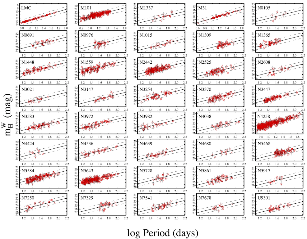
Figure 9: HST NIR Wesenheit Cepheid $P$–$L$ relations. The Cepheid magnitudes are shown for 37 SN Ia hosts, M31, and 2 of the 3 possible distance-scale anchors (LMC and NGC 4258). The uniformity of the photometry and metallicity reduces systematic errors along the distance ladder. A single slope is shown and used for the baseline, but we also allow for a break (two slopes) as well as limited period ranges in some analysis variants.

4.6 Period–Luminosity Relations

Fig. 9 shows the 40 individual Cepheid host $m^{W}_{H}$ $P$–$L$ relations (not including the MW as explained above) for a period range of $5\!<\!P\!<\!120$ d fitted with a common slope. Before combining the results of many hosts in a global analysis, we examine in Fig. 10 the independently-fitted slopes of the $m_{H}^{W}$ $P$–$L$ relations across all Cepheid hosts.

The slopes are all consistent (at the $\sim 2\sigma$ level) with a mean in the range of $-3.27$ to $-3.30$ mag dex^-1. The most tightly constrained slope comes from the LMC with $-3.284\pm 0.017$ mag dex^-1, mostly from the ground sample. Overall, we see no evidence to reject the null hypothesis of a single slope. There have been claims in the past of a break at $P\approx 10$ d which we will consider as a variant of the primary analysis in the next section. However, the mean slopes from these data below and above $P=10$ d are $-3.33\pm 0.02$ and $-3.21\pm 0.06$ mag dex^-1 (respectively), a difference of $1.8\sigma$; individual hosts with the strongest constraint (LMC and the M31 PHAT sample) show slope changes at $P=10$ d in opposite directions. Furthermore, formal uncertainties in these slopes are somewhat underestimated because of the uneven sampling of periods between hosts. A Monte Carlo analysis (bootstrap resampling with replacement) from hosts with the largest samples of Cepheids shows variations owing to uneven period sampling increases the formal slope uncertainty typically by 10% and up to 35% for the LMC. We find that the metallicity dependence has a negligible effect on the mean slope. Therefore, in the following we will consider a single slope for $5<P<120$ d in our baseline analysis, but we analyze the impact of a break or limited period range on the determination of H₀ as variants of the baseline analysis.

4.7 Geometric Distance Priors

We make use of the geometric distances to NGC 4258 from masers (Reid:2019) of $\mu_{\textsc{n4258}}=29.398\pm 0.032$ mag, the LMC from DEBs (Pietrzynski:2019) of $\mu_{\textsc{lmc}}=18.477\pm 0.0263$ mag, and the SMC from DEBs (Graczyk:2020) in the form of $\Delta\mu_{\textsc{lmc-smc}}=0.500\pm 0.017$ mag, as well as the MW Gaia EDR3 and HST spatial-scan parallaxes discussed in §4.1. These are all given in Table 4.

4.8 SN Magnitudes

We adopt standardized SN Ia magnitudes $m_{B}^{0}$ from the Pantheon+ analysis (Scolnic:2021; Brout:2022), where the value $m_{B,i}^{0}$ is a measure of the maximum-light apparent $B$-band brightness of a SN Ia in the i-th host at the time of $B$-band peak, corrected to the fiducial color and luminosity determined for each SN Ia from its multiband light curves and a light-curve-fitting algorithm. We use the uncertainties and covariance of $m_{B}^{0}$ as given by the Pantheon+ analysis. The SN Ia covariance matrix has substantial off-diagonal terms and is displayed in Fig. 11. An improvement in the current analysis of calibrator SNe Ia over R16 is our use of multiple SN light-curve datasets for most calibrators, 77 sets in all for 42 SNe Ia, a mean of $\sim 2$ independent sets per SN, reducing measurement errors (not intrinsic scatter, which is covariant among multiple samples of the same SN) by a mean factor of 1.4. These datasets are given in Scolnic:2021.

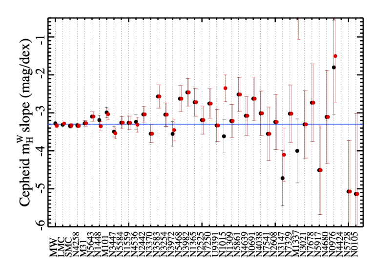
Figure 10: Independent determinations of the slope of the $P$–$L$ relation in each host plotted in order of precision. Black (red) points are after (before) outlier rejection. We find that the slopes are consistent with a single value of $-3.27$ to $-3.30$ as indicated by the blue line. The most metal-poor (SMC) and metal-rich (MW) also have consistent slopes. Error bars are for the fit error only and do not include uneven period sampling or background covariance. The large change in slope for Mrk 1337 was due to the relatively small sample size and rejection of a few Cepheids far from its center.

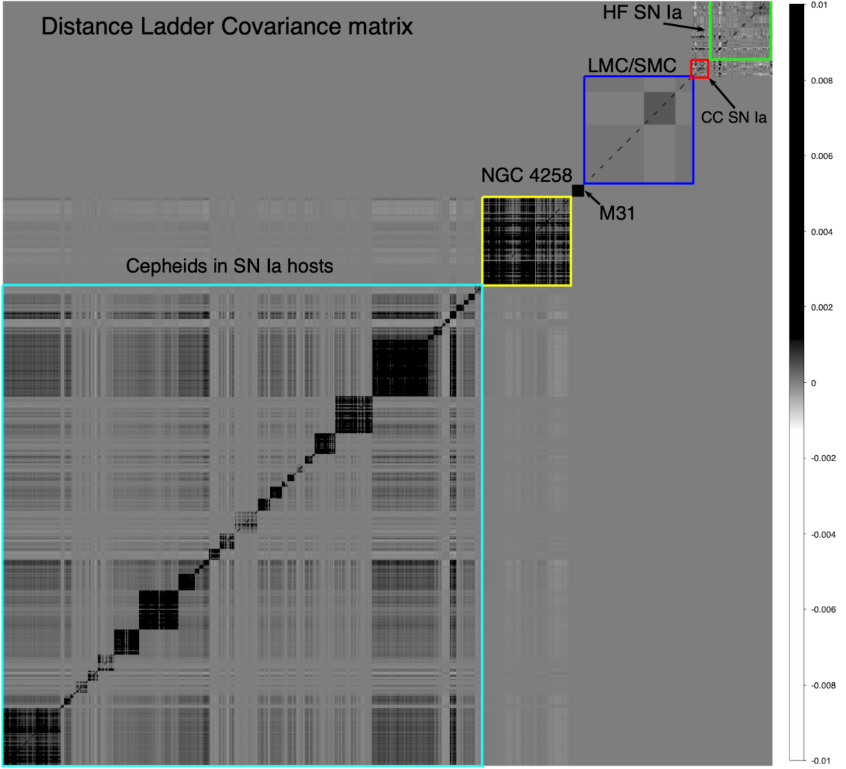
Figure 11: Distance ladder covariance matrix. Graphical representation of the covariance matrix of measurements with values applicable to different sources indicated. The covariance matrix contains past sources of systematic error that propagate here as error in the fit. Among Cepheid hosts, square blocks along the diagonal indicate the background covariance within a host (Eq. 8) while the covariance pattern between hosts farther off the diagonals comes from the covariance of the metallicity scale (Eq. 9). The SN-SN covariance is characterized in the Pantheon+ analysis (Scolnic:2021; Brout:2022).

Table 5: Fits for H₀

Fit	Variant	$\chi^{2}_{dof}$	N	H0	b	$\gamma$	$M_{W}^{0}$	$M_{B}^{0}$	$a_{b}$
1	Baseline	1.03	3445	73.04 1.01	-3.299 0.015	-0.217 0.046	-5.894	-19.253	0.714158
Cepheid Clipping Variants §6.1
2	global $\sigma_{\textrm{clip}}=3.3$	1.03	3446	73.19 1.01	-3.298 0.015	-0.216 0.046	-5.891	-19.249	0.714174
3	individual PL $\sigma_{\textrm{clip}}=3.3$	0.99	3370	73.25 1.02	-3.296 0.015	-0.201 0.045	-5.893	-19.248	0.714315
4	tight:one-by-one MAD $\sigma_{\textrm{clip}}=3.0$	0.99	3429	73.12 1.01	-3.299 0.015	-0.220 0.045	-5.893	-19.251	0.714175
5	tight:global $\sigma_{\textrm{clip}}=3.0$	0.99	3432	73.22 1.01	-3.298 0.015	-0.215 0.045	-5.891	-19.248	0.714194
6	loose:global $\sigma_{\textrm{clip}}=5.0$	1.16	3475	73.34 1.01	-3.294 0.016	-0.221 0.049	-5.888	-19.244	0.714183
7	loose:one-by-one MAD $\sigma_{\textrm{clip}}=5.0$	1.15	3474	73.42 1.01	-3.295 0.016	-0.222 0.048	-5.888	-19.242	0.714178
8	loose:individual PL $\sigma_{\textrm{clip}}=5.0$	1.05	3397	73.35 1.01	-3.296 0.015	-0.202 0.046	-5.892	-19.244	0.714257
9	none	1.23	3481	73.41 1.01	-3.290 0.016	-0.206 0.050	-5.885	-19.242	0.714248
Geometric Anchors Variants §6.2
10	N4258	1.06	3454	72.51 1.54	-3.294 0.015	-0.204 0.051	-5.905	-19.269	0.714174
11	Milky Way	1.03	3446	73.02 1.19	-3.298 0.015	-0.208 0.051	-5.895	-19.254	0.714179
12	LMC	1.03	3446	73.59 1.36	-3.298 0.015	-0.208 0.051	-5.878	-19.237	0.714178
13	N4258+MW	1.03	3446	73.00 1.09	-3.298 0.015	-0.207 0.050	-5.895	-19.254	0.714171
14	N4258+LMC	1.03	3446	73.35 1.17	-3.299 0.015	-0.211 0.050	-5.885	-19.244	0.714179
15	MW+LMC	1.03	3446	73.25 1.05	-3.298 0.015	-0.216 0.046	-5.889	-19.247	0.714169
Cepheid Dust-Color Treatment Variants §6.3
16	Fitzpatrick 99 law $R_{V}=2.5$	1.03	3446	73.24 1.00	-3.291 0.015	-0.209 0.046	-5.850	-19.247	0.714171
17	CCM law $R_{V}=3.1$	1.04	3445	73.09 1.00	-3.310 0.015	-0.226 0.046	-5.957	-19.252	0.714183
18	Nataf law $R_{V}=3.3$	1.03	3445	73.32 0.99	-3.276 0.015	-0.204 0.046	-5.804	-19.245	0.714141
19	$R_{W}$ free global	1.03	3446	73.40 1.02	-3.286 0.016	-0.204 0.046	-5.835	-19.242	0.714167
20	intrin. col. subtr. F99 $R_{V}=3.3$	1.03	3446	73.13 1.01	-3.201 0.015	-0.218 0.046	-5.604	-19.250	0.714170
21	intrin. col. subtr. F99 $R_{V}=$ free	1.03	3446	73.34 1.01	-3.201 0.015	-0.206 0.046	-5.582	-19.244	0.714170
22	intrin. col. subtr. $R_{V}$(host mass-SFR)	1.05	3446	73.85 1.02	-3.202 0.015	-0.228 0.046	-5.605	-19.229	0.714230
23	None($A_{H}$ values assumed to cancel)	1.11	3437	74.78 1.03	-3.188 0.016	-0.115 0.048	-5.434	-19.201	0.714086
PL Break/span Variants §6.4
24	Break at $P=10$ d	1.03	3444	72.68 1.04	-0.10 0.05	-0.222 0.046	-5.887	-19.264	0.714151
25	Only use $P>10$ d	1.06	3004	73.15 1.11	-3.337 0.023	-0.169 0.051	-5.861	-19.250	0.714158
26	Only use $P<60$ d	0.93	3699	73.99 1.04	-3.261 0.011	-0.236 0.044	-5.898	-19.226	0.714276
M31 Cepheid Sampl Variants §6.5
27	M31 PHAT sample	1.02	3854	73.21 1.00	-3.297 0.013	-0.234 0.044	-5.893	-19.248	0.714184
28	M31 PHAT sample +Break at $P=10$ d	1.02	3852	72.74 1.03	-0.07 0.04	-0.240 0.044	-5.891	-19.262	0.714156
Metallicity Variants §6.6
29	no metallity dependence	1.04	3446	73.52 1.01	-3.296 0.015	$\dots$	-5.860	-19.239	0.714194
30	PP04 metallicity scale	1.04	3446	72.84 1.00	-3.297 0.015	-0.166 0.042	-5.883	-19.259	0.714162
TRGB Inclusion Variants §6.7
31	adds EDD TRGB+N4258tip	1.03	3457	72.76 0.95	-3.301 0.015	-0.197 0.045	-5.891	-19.262	0.714253
32	adds CCHP TRGB+N4258tip	1.03	3457	72.29 0.94	-3.304 0.015	-0.208 0.046	-5.894	-19.276	0.714254
Hubble Flow Sample Variants §6.8
33	all host types $0.0233<z<0.15$	1.03	3652	73.32 0.99	-3.298 0.015	-0.216 0.046	-5.891	-19.246	0.714479
34	highz:all host types $0.0233<z<0.80$	1.00	4483	73.68 0.98	-3.298 0.015	-0.216 0.045	-5.891	-19.244	0.716225
35	skip local alltypes $0.06<z<0.15$	1.04	3318	73.35 1.06	-3.298 0.015	-0.217 0.046	-5.891	-19.245	0.714311
36	highz:skip local alltypes $0.06<z<0.8$	1.00	4149	73.90 1.01	-3.298 0.015	-0.217 0.045	-5.891	-19.242	0.716991
37	highmass:hubble flow host logmass$>10$	1.04	3304	72.97 1.04	-3.298 0.015	-0.217 0.046	-5.891	-19.251	0.713297
Calibrator Sample Variants §6.9
38	complete calibrator sample $z<0.011$	1.03	3446	73.30 1.02	-3.298 0.015	-0.217 0.046	-5.891	-19.245	0.714191
39	complete sample $z<0.011$+TRGB	1.04	3458	72.88 0.95	-3.301 0.015	-0.196 0.045	-5.888	-19.258	0.714297
40	highmass:calibrator host logmass$>10$	1.03	3445	73.54 1.10	-3.296 0.015	-0.214 0.046	-5.891	-19.238	0.714201
41	Use least crowded half	1.02	3446	73.34 1.16	-3.297 0.015	-0.223 0.046	-5.892	-19.246	0.714597
42	Use most crowded half hosts	1.02	3445	73.35 1.37	-3.293 0.015	-0.215 0.046	-5.891	-19.243	0.714063
43	only 19 hosts from R16	1.02	3446	73.47 1.17	-3.297 0.015	-0.229 0.046	-5.893	-19.242	0.714505
44	only hosts since R16	1.02	3445	73.07 1.31	-3.293 0.015	-0.210 0.046	-5.890	-19.252	0.714178
45	closer half hosts $m_{b}<13$	1.03	3446	73.07 1.16	-3.295 0.015	-0.219 0.046	-5.891	-19.252	0.714191
Excluded SN Surveys Variants §6.10
46	No SDSS SNe	1.03	3446	72.90 1.02	-3.298 0.015	-0.217 0.046	-5.891	-19.249	0.712428
47	No CSP SNe	1.02	3445	73.43 1.06	-3.298 0.015	-0.217 0.046	-5.891	-19.246	0.715130
48	No literature SNe	1.03	3446	73.47 1.05	-3.298 0.015	-0.213 0.046	-5.890	-19.240	0.714072
49	No LOSS SNe	1.02	3447	73.26 1.04	-3.297 0.015	-0.213 0.046	-5.891	-19.251	0.715022
50	No Swift SNe	1.03	3445	73.09 1.02	-3.297 0.015	-0.217 0.046	-5.891	-19.248	0.713551
51	No CfA1/2 SNe	1.03	3446	73.03 1.03	-3.298 0.015	-0.218 0.046	-5.891	-19.250	0.713464
52	No CfA3/4 SNe	1.03	3447	73.31 1.02	-3.298 0.015	-0.214 0.046	-5.891	-19.245	0.714257
53	No Foundation SNe	1.01	3446	73.46 1.03	-3.298 0.015	-0.217 0.045	-5.891	-19.241	0.714196
54	No pre-2000 SNe	1.02	3446	73.20 1.09	-3.297 0.015	-0.218 0.046	-5.891	-19.245	0.713530
SN Fitting Variants §6.11
55	SN scatter monochromatic	1.00	3444	73.54 1.08	-3.296 0.015	-0.223 0.045	-5.892	-19.238	0.714067
Peculiar Velocity Variants §6.12
56	2MRS	1.03	3446	73.12 1.01	-3.298 0.015	-0.216 0.046	-5.891	-19.249	0.713775
57	CMB frame z	1.04	3446	72.70 1.00	-3.298 0.015	-0.216 0.046	-5.891	-19.249	0.711260
58	$q_{0}=-0.52$	1.03	3446	73.19 1.01	-3.298 0.015	-0.216 0.046	-5.891	-19.249	0.714149
59	$q_{0}=-0.52$ all highz	1.00	4483	73.65 0.98	-3.298 0.015	-0.216 0.045	-5.891	-19.244	0.715950
Optical Wesenheit Variants §6.13
60	optical Wesenheit clipping=one-by-one	0.94	3626	72.70 1.03	-3.299 0.010	-0.248 0.041	-5.858	-19.264	0.714413
61	optical Wesenheit clipping=global	0.94	3626	72.90 1.03	-3.291 0.010	-0.247 0.041	-5.857	-19.259	0.714417
62	optical Wesenheit F99 $R_{V}=2.5$	0.92	3618	73.20 1.03	-3.230 0.010	-0.202 0.041	-5.623	-19.249	0.714359
63	optical Wesenheit CCM $R_{V}=3.1$	0.97	3626	72.46 1.03	-3.335 0.010	-0.270 0.042	-6.020	-19.272	0.714469
64	optical Wesenheit N4258 only	0.92	3623	74.85 2.31	-3.291 0.010	-0.211 0.045	-5.797	-19.201	0.714429
65	optical Wesenheit MW only	0.93	3623	71.93 1.15	-3.291 0.010	-0.211 0.045	-5.883	-19.288	0.714421
66	optical Wesenheit LMC only	0.92	3623	74.26 1.39	-3.291 0.010	-0.211 0.045	-5.814	-19.218	0.714416
67	optical Wesenheit+TRGB	0.94	3638	72.15 0.94	-3.301 0.010	-0.239 0.041	-5.858	-19.281	0.714385

Table 6: Approximations for Distance Parameters

N	Host	SN	$m_{B,i}^{0}$	$\sigma$	$\mu_{\rm Ceph}^{a}$	$\sigma$	$M_{B,i}^{0}$	$\sigma$	$\mu_{\rm host}^{b}$	$\sigma$	$R^{c}$
			[mag]
1	M101	2011fe	9.7800	0.115	29.193	0.039	-19.413	0.122	29.178	0.041	0.44
2	M1337	2006D	13.655	0.106	32.922	0.124	-19.267	0.163	32.920	0.123	0.43
3	N0105	2007A	15.250	0.133	34.531	0.253	-19.281	0.286	34.527	0.250	0.37
4	N0691	2005W	13.602	0.139	32.846	0.109	-19.244	0.177	32.830	0.109	0.42
5	N0976	1999dq	14.250	0.103	33.719	0.151	-19.468	0.183	33.709	0.149	0.30
6	N1015	2009ig	13.350	0.094	32.570	0.075	-19.220	0.120	32.563	0.074	0.46
7	N1309	2002fk	13.209	0.082	32.546	0.060	-19.337	0.102	32.541	0.059	0.38
8	N1365	2012fr	11.900	0.092	31.379	0.057	-19.479	0.108	31.378	0.056	0.46
9	N1448	2001el	12.254	0.136	31.290	0.037	-19.036	0.141	31.287	0.037	0.41
10	N1448	2021pit	11.752	0.200	31.290	0.037	-19.538	0.203	31.287	0.037	0.41
11	N1559	2005df	12.141	0.086	31.501	0.062	-19.360	0.106	31.491	0.061	0.35
12	N2442	2015F	12.234	0.082	31.457	0.065	-19.223	0.105	31.450	0.064	0.36
13	N2525	2018gv	12.728	0.074	32.067	0.100	-19.339	0.124	32.051	0.099	0.39
14	N2608	2001bg	13.443	0.166	32.629	0.155	-19.186	0.227	32.612	0.154	0.39
15	N3021	1995al	13.114	0.116	32.474	0.160	-19.360	0.198	32.464	0.158	0.34
16	N3147	2021hpr	13.843	0.159	33.044	0.165	-19.201	0.229	33.014	0.165	0.45
17	N3147	1997bq	13.821	0.141	33.044	0.165	-19.223	0.217	33.014	0.165	0.45
18	N3147	2008fv	13.936	0.200	33.044	0.165	-19.108	0.260	33.014	0.165	0.45
19	N3254	2019np	13.201	0.074	32.332	0.077	-19.130	0.107	32.331	0.076	0.52
20	N3370	1994ae	12.937	0.082	32.123	0.052	-19.186	0.097	32.120	0.051	0.33
21	N3447	2012ht	12.736	0.089	31.939	0.035	-19.203	0.096	31.936	0.034	0.40
22	N3583	ASASSN-15so	13.509	0.093	32.808	0.081	-19.299	0.123	32.804	0.080	0.34
23	N3972	2011by	12.548	0.094	31.644	0.090	-19.096	0.130	31.635	0.089	0.46
24	N3982	1998aq	12.252	0.078	31.724	0.072	-19.472	0.106	31.722	0.071	0.36
25	N4038	2007sr	12.409	0.106	31.615	0.117	-19.206	0.158	31.603	0.116	0.57
26	N4424	2012cg	11.487	0.192	30.856	0.130	-19.369	0.232	30.844	0.128	0.87
27	N4536	1981B	11.551	0.133	30.838	0.051	-19.287	0.142	30.835	0.050	0.49
28	N4639	1990N	12.454	0.124	31.818	0.085	-19.364	0.150	31.812	0.084	0.48
29	N4680	1997bp	13.173	0.205	32.606	0.208	-19.433	0.292	32.599	0.205	0.48
30	N5468	1999cp	13.880	0.080	33.120	0.075	-19.240	0.110	33.116	0.074	0.39
31	N5468	2002cr	13.993	0.072	33.120	0.075	-19.127	0.104	33.116	0.074	0.39
32	N5584	2007af	12.804	0.079	31.775	0.053	-18.971	0.095	31.772	0.052	0.36
33	N5643	2013aa	11.252	0.079	30.569	0.050	-19.317	0.093	30.546	0.052	0.39
34	N5643	2017cbv	11.208	0.074	30.569	0.050	-19.362	0.089	30.546	0.052	0.39
35	N5728	2009Y	13.514	0.115	33.116	0.207	-19.602	0.236	33.094	0.205	0.58
36	N5861	2017erp	12.945	0.107	32.232	0.101	-19.287	0.147	32.223	0.099	0.33
37	N5917	2005cf	13.079	0.095	32.363	0.122	-19.284	0.154	32.363	0.120	0.47
38	N7250	2013dy	12.283	0.178	31.628	0.126	-19.345	0.218	31.628	0.125	0.49
39	N7329	2006bh	14.030	0.079	33.274	0.116	-19.244	0.140	33.246	0.117	0.39
40	N7541	1998dh	13.418	0.128	32.504	0.121	-19.086	0.176	32.500	0.119	0.30
41	N7678	2002dp	14.090	0.093	33.196	0.155	-19.106	0.181	33.187	0.153	0.39
42	U9391	2003du	13.525	0.084	32.849	0.068	-19.324	0.108	32.848	0.067	0.44

Note. — (a) Approximate, Cepheid-based distance derived without inclusion of the SNe in a given host. (b) Cepheid-based distance derived without inclusion of any SN in any host. (c) Empirical host reddening ratio derived from mass and star-formation rate (SFR) using EDA (§6.3). (d) $m_{B,i}^{0}$ and error given are an approximation, the simple average from one or more SN surveys

Figure 12: Complete distance ladder. The simultaneous agreement of distance pairs: geometric and Cepheid-based (lower left), Cepheid- and SN-based (middle), and SN- and redshift-based (top right) provides the measurement of H₀. For each step, geometric or calibrated distances on the abscissa serve to calibrate a relative distance indicator on the ordinate through the determination of $M_{B}$ or H₀. Results shown are an approximation to the global fit as discussed in the text. Red SN points are at $0.0233<z<0.15$, with the lower-redshift bound producing the appearance of asymmetric residuals when plotted against distance.

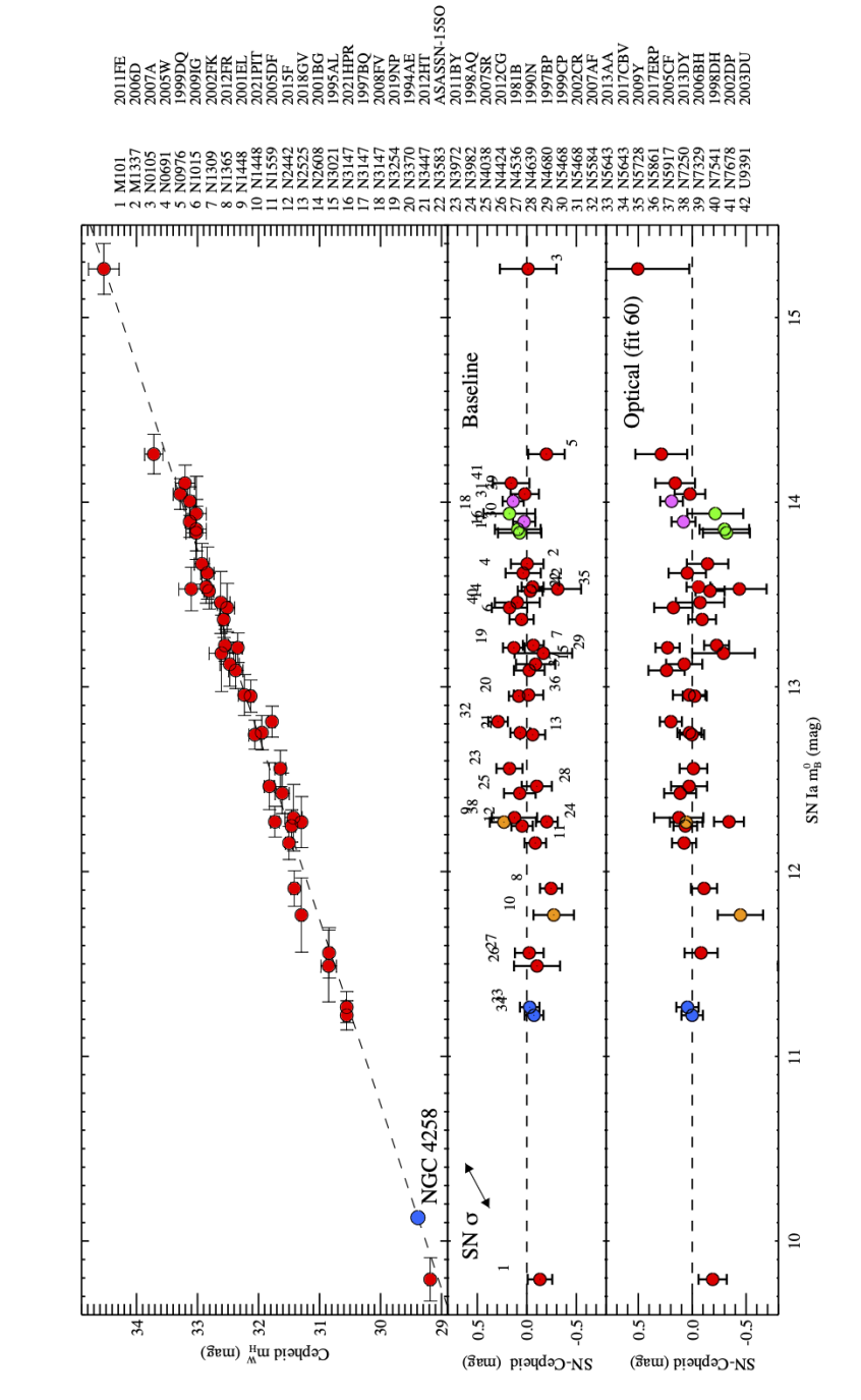
Figure 13: Comparison of SN and Cepheid distance measures on the second rung of the distance ladder, and residuals (middle). Because the residual panel includes SN measures on both axes, residuals are convolved by the SN error arrow as indicated. An alternate plot with Cepheids on the abscissa is shown in Fig. 12. SNe that share a common host are identified with various colors. We find no significant trend ($<1.5\sigma$) in this space. Results shown are an approximation to the global fit as discussed in the text. The lower panel replaces the NIR-based Cepheid magnitudes with the optical only from Fit 60.

5 The Local Value of H₀, the Baseline

Our calibrator sample contains 42 SNe Ia in the 37 Cepheid hosts presented in the previous section and 277 SNe Ia in the Hubble flow, all the objects at $0.0233\!<\!z\!<\!0.15$ from the Pantheon+ sample which pass the same quality cuts and are in late-type hosts like the Cepheid calibrators. Criteria for inclusion in the sample used to measure the Hubble flow and variations are further considered in §6.7.

Our baseline (best) analysis includes the full array of constraints on our model and what we assess to be the optimal choices (considering a wide range of alternatives in §6) in the treatment of the available data. Its results, derived from the optimization of $\chi^{2}$ in Equation (6), are given in the first line of Table 5, which also provides the best-fit parameters. This fit gives a $\chi^{2}_{\textrm{dof}}=$ $1.03$  with $N=3445$ degrees of freedom, with Cepheid slope, metallicity, and luminosity parameters $b_{W}=$ $-3.299\pm 0.015$ mag/dex, $Z_{W}=$ $-0.217\pm 0.046$ mag/dex, and $M_{H,1}^{W}=$ $-5.894\pm 0.017$ mag. These parameters are similar to those found by R16 and updated by R19, with small increases in the absolute values of the slope of the $P$–$L$ relation (from $-3.26\pm 0.03$ in R16) and the metallicity dependence (from $-0.17\pm 0.06$ in R19). Additional “nuisance” parameters in the baseline fit are $\Delta\mu_{\rm N4258}=-0.013\pm 0.022$ mag and $\Delta\mu_{\rm LMC}=0.010\pm 0.019$ mag. Table 6 provides individual host distances and SN parameters. Fig. 12 displays the baseline data, fit, and residuals, while Fig. 13 provides more details about the central panel of the preceding figure.

The fiducial SN absolute magnitude parameter applicable to the Pantheon+ standardization (Scolnic:2021; Brout:2022) is $M_{B}^{0}=$ $-19.253\pm 0.027$ mag. The value of the Hubble constant derived from the baseline fit is H₀=$73.04\pm 1.01$ km s^-1 Mpc^-1. Including an additional systematic uncertainty from the analysis variants as discussed in §6.14 yields

$${\textbf{H}}\bm{{}_{0}}\bm{=}\bm{73.04\pm 1.04}\textbf{\ km\ s}\bm{{}^{-1}}\ \textbf{Mpc}\bm{{}^{-1}}\ \textbf{(baseline with systematics)}.$$ (10)

The determination of H₀ in the measured space is $5\,\log$ H₀ $=9.318\pm 0.031$ (with systematics) where the errors are symmetric in log space and slightly asymmetric for H₀ with errors of ($-0.98$ and $+1.03$ for the fit). The full difference from the Planck+$\Lambda$CDM prediction of H${}_{0}=67.4\pm 0.5$ (Planck:2018) in units of $\Delta 5\,\log$ H₀ is $0.176\pm 0.035$ mag (errors in quadrature), a difference of 5.0$\sigma$ (one in 3.5 million).

The dispersion (weighted by the measurement errors) between the 42 calibrator SNe Ia and Cepheids is $\sigma=0.130$ mag which is equivalent to (albeit slightly lower than) the 0.135 mag dispersion between the SN magnitudes and redshifts of the Hubble-flow sample. We would expect these dispersions to be comparable (as they are) because the additional sources of scatter independent of SNe and applicable to the two comparisons (Cepheid distance errors and peculiar velocities) are both subdominant to SN scatter. From these dispersions and the good global $\chi^{2}$ we conclude that there is no unexplained variance in the baseline fit beyond the intrinsic scatter of SNe Ia and the intrinsic width of the Cepheid instability strip.

5.1 Markov Chain Monte Carlo (MCMC) Sampling

To check the preceding calculation using a different methodology, we performed MCMC sampling. Our likelihood function is

$$p(q\mid L,C,y)\propto p(q)\ p(L,C,y\mid q)\ ,$$ (11)

where the $p(L,C,y\mid q)$ is a Gaussian likelihood based on the covariance matrix $C$; if $C$ is diagonal, $C_{ij}=\sigma_{i}^{2}\delta_{ij}$, it has the form

$$p(L,C,y\mid q)=\prod_{i}\frac{1}{\sqrt{2\pi}\sigma_{y}}\exp\left[\frac{-(y_{i}-y_{\rm{fit},i})^{2}}{2\sigma_{y}^{2}}\right]\ .$$ (12)

Since the covariance matrix $C$ is independent of $q$ in our setup, Equation 11 can be simplified to

$$p(q|L,C,y)\propto p(q)\exp\left(-\frac{1}{2}\sum_{i}\chi_{i}^{2}\right)\ .$$ (13)

For the calculation of $\chi^{2}$, we followed the method described in Equation (6). For numerical accuracy, we substituted $C^{-1}$ with an inverse of Cholesky-decomposed lower triangular matrix $\tilde{C}_{L}^{-1}$ (which satisfies $\tilde{C}_{L}\tilde{C}_{L}^{-1}=I$ and $\tilde{C}_{L}\tilde{C}_{L}^{T}=C$):

$$\chi^{2}=\left(y-L\cdot q\right)\tilde{C}_{L}^{-1}\left(y-L\cdot q\right)\ .$$ (14)

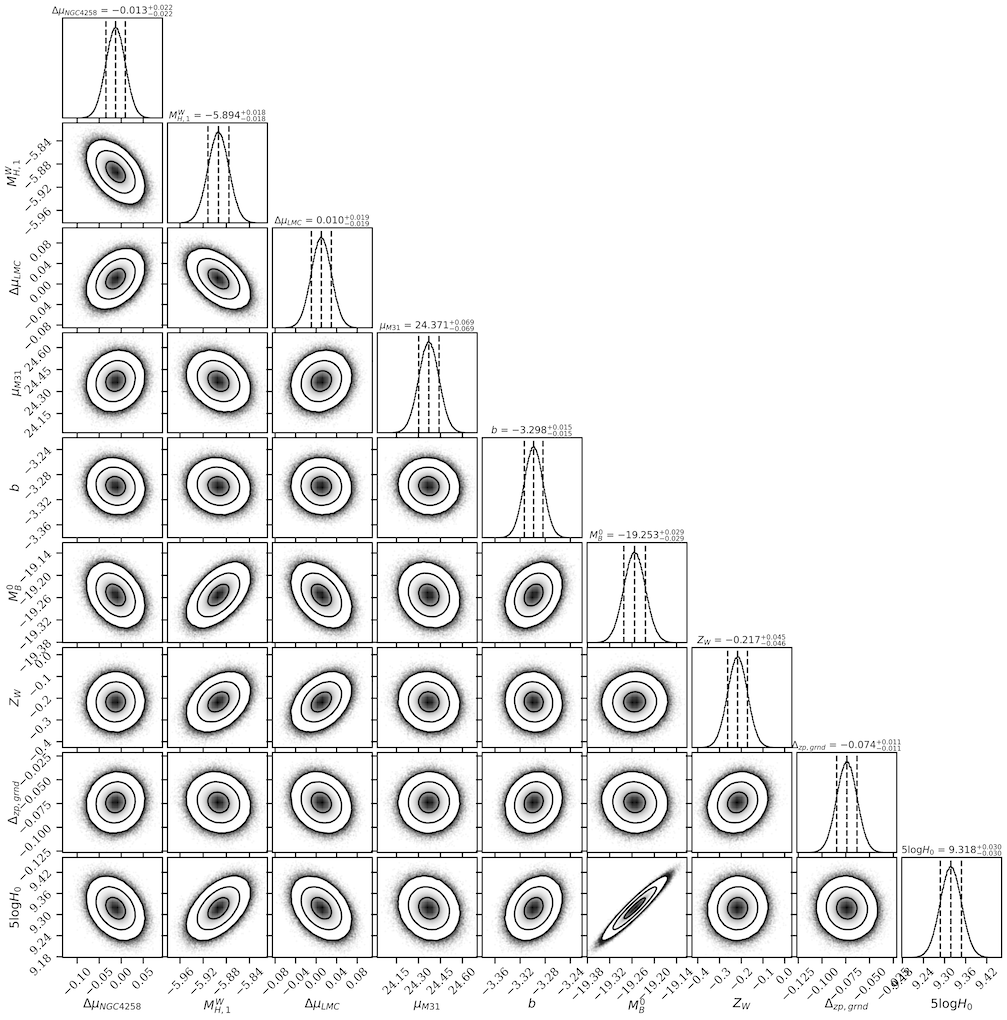
Figure 14: MCMC sampling of the $\chi^{2}$ statistic of the global fit showing all free parameters except the individual host distances. Contours are 1$\sigma$, 2$\sigma$, and 3$\sigma$ confidence regions. We find that the means and uncertainties agree very well with the analytical minimization of $\chi^{2}$.

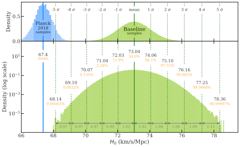
Figure 15: Extended MCMC sampling of the posterior for H₀ to measure out to the $\pm 5\sigma$ confidence level. The upper panel shows the probability density for the baseline from SH0ES and from the Planck:2018 chains. The bottom panel shows the log of the probability density to improve the ability to see the tails. We note some asymmetry to the distribution, with intervals on the low-H₀ side a little smaller than on the high side, as the measurements are Gaussian in magnitudes and in $5\,\log$ H₀, hence slightly skewed in H₀.

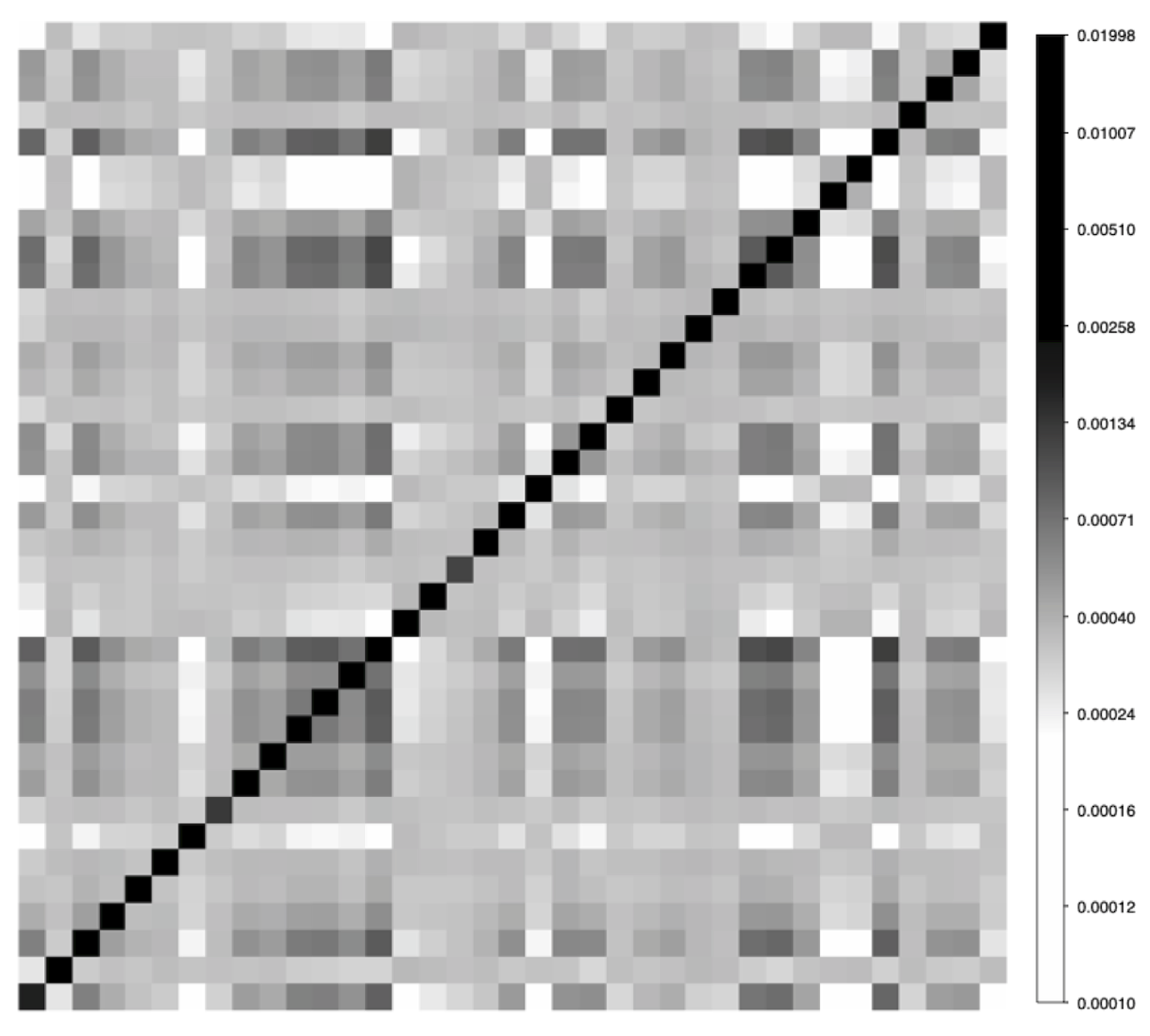
Figure 16: Host distance ($\mu_{\rm host}$) covariance matrix. This is the covariance for the baseline set of 37 hosts derived only from the first two rungs and without the use of any SN Ia data. The nonzero off-diagonal terms result from common anchors, common parameters of the Cepheid $P$–$L$ relation, and covariance of the metallicity scale. The systematic uncertainty in all host distances may be measured from the square root of the level of the off-diagonal elements and is 0.019 mag, or 0.9% in distance.

As a “neutral” prior, we chose the uniform distribution

$$q_{i}\sim\rm{Uniform}(\mu_{i}-10\sigma_{i},\mu_{i}+10\sigma_{i}),$$ (15)

which is centered at the results from the analytical result. Its width is set to be sufficiently ($20\times$) larger than the estimated standard deviation from linear regression $\sigma$. We find that this range is more than enough to allow determination of median and standard deviation of the resulting population from $\mu$ and $\sigma$.

We used the Python package emcee (emcee_2013) to perform sampling under conditions mentioned above. The initial states are uniformly distributed in the prior range (Eq. 14) for a total of 100 walkers. The convergence is monitored using emcee’s recommended method to estimate the autocorrelation time $\tau$, which employs a method originally proposed by Goodman_2010_autocorr. The burn-in time is set to be $5\tau$ to allow chains to fully converge.

The convergence of the sampled distribution is checked visually and by the estimated autocorrelation time value. We required the total number of chains after burn-in $N$ to satisfy $N>100\tau$ before any visual inspection for convergence is performed. The samples used in the final analysis are contained well within the inner region of the initial states for all parameters, indicating that our choice of prior size did not affect the final result.

The results for selected parameters are shown in Fig. 14. All parameters exhibit Gaussian-like posterior probability density functions (PDFs), which indicates that the results from the linear-regression method are a good representation of the results from this project. The locations of Gaussian-equivalent percentiles (i.e., the locations at which the same relative volume is met) in our sample suggest that the samples in H₀ are more broadly distributed toward larger values (right-hand side; RHS) than smaller ones (left-hand side; LHS), a consequence of Gaussian errors in magnitudes of $5\,\log$ H₀, with the mean distances between each line $\bar{\sigma}_{R}=1.06$ on the RHS and $\bar{\sigma}_{L}=0.98$ on the LHS (toward lower H₀), similar to the analytical results.

More than 120 million samples were used for the baseline fit to delineate the position of the 5$\sigma$ confidence interval for H₀, as shown in Fig. 15. The calculated values of $\sigma$, whose mean is $\bar{\sigma}_{\rm{all}}=1.02$, contains the estimated uncertainty from the linear-regression method $\sigma_{\rm{reg}}=1.01$, hence showing a full consistency between two methods. Using these three values ($\bar{\sigma}_{L}$, $\bar{\sigma}_{\rm{all}}$, and $\sigma_{\rm{reg}}$), and regarding the $50^{\rm{th}}$ percentile value as the most probable value for the first two cases, our results are H${}_{0,\rm{MCMC-L}}=73.04\pm 0.98$, H${}_{0,\rm{MCMC-all}}=73.42\pm 1.02$, and H${}_{0,\rm{reg}}=73.04\pm 1.01$ km s^-1 Mpc^-1.

The significance of the discrepancy between our results and those of Planck:2018, H${}_{0,\rm{Planck}}=67.4\pm 0.5$, are $5.1\sigma$, $4.9\sigma$, and $5.0\sigma$, respectively.

5.2 Simultaneous Constraints on H₀ and the Expansion History

This section illustrates an approach to simultaneously measure H₀ and the expansion history for an arbitrary form of H$(z)$, using the full covariance of the datasets.

The “near-field” determination of H₀ in the preceding section is quite insensitive to specific knowledge of the recent expansion history because the mean redshift at which the measurement is made, $\langle z\rangle=0.055$, is low. Yet to make the measurement more precise at even these small redshifts, in the prior section we accounted for the derivative of the expansion history in Equation (4) through the empirical derivative of H$(z)$ measured from higher-redshift SNe Ia, $q_{0}$. We set $q_{0}=-0.55$ as this is historically a good fit to high-redshift SNe Ia. This empirical approach is fully independent of the CMB, so an independent comparison of H₀ to the CMB with $\Lambda$CDM is appropriate.

However, to consider less-conventional expansion histories such as a rapid change in H$(z)$ together with the measured value of H₀, as may be undertaken in the effort to find a resolution of the Hubble tension, it might be necessary and it is certainly more reliable to explicitly account for the dependence of H₀ on the form of the expansion history, H$(z)$, at low redshifts (Efstathiou:2021; Camarena:2021). Furthermore, there is covariance in the measurements of SNe Ia, whether in Cepheid hosts or at moderate redshifts (Scolnic:2018; Dhawan:2020), and it is necessary to account for this when SNe Ia are used simultaneously to measure H₀ and the recent expansion history.

It is important to recognize that standardized SN Ia data can provide only relative distance measurements between all SNe measured within the same standardization scheme, with SN parameters, uncertainties, and covariance with values relevant within the context of the algorithm used to standardize the SNe. Therefore, to avoid inconsistencies between SN standardization schemes or loss of knowledge of measurement covariance, one would ideally make full use of all relevant SN data simultaneously to determine absolute quantities. A straightforward and reliable path is to use the set of absolute distances to SN hosts (their uncertainties and covariance) derived from only the first two rungs without the use of any SN data, together with a consistently standardized set of SNe (in these hosts and in the Hubble flow), to determine H₀ and H$(z)$ simultaneously, the so-called “forward” direction. Or, one could alternatively follow an “inverse” approach, starting with CMB data and using the best-fit $\Lambda$CDM model to calibrate the distance–redshift relation of SNe including the predicted distances of nearby hosts of SNe Ia and Cepheids (or TRGB). Here we follow the forward approach.

For the set of SN hosts with calibrated distances (using only the first two rungs of the distance ladder), the dereddened absolute distance modulus $\mu_{0}$ is given by

$$\mu_{0,\textrm{host}}-m_{B}=M_{B},$$ (16)

with terms given in Equation (3). We then have a second set of SNe with cosmological redshifts $z>0$,

$$m_{B}=5\,\log\,cz\left\{1+{\frac{1}{2}}\left[1-q_{0}\right]{z}-{\frac{1}{6}}\left[1-q_{0}-3q_{0}^{2}+j_{0}\right]z^{2}+O(z^{3})\right\}-5\,\log\,{\rm H}_{0}+M_{B}+25.$$ (17)

.

The two leading terms on the right-hand side of Equation (17) can be replaced with any empirical or cosmological model for H$(z)$, such as the example of $\Lambda$CDM with dark energy equation-of-state parameter $w$ and mass density $\Omega_{M}$,

$$m_{B}=5\,\log\,\left[c{\rm H}_{0}^{-1}(1+z)\int_{0}^{z}{\frac{dz^{\prime}}{E(z^{\prime})}}\right]+25+M_{B},$$ (18)

where

$$E(z)\equiv\left\{\Omega_{m}(1+z^{\prime})^{3}+(1-\Omega_{m})\times\exp\left[+3\int_{0}^{\ln(1+z)}d\ln(1+z^{\prime})(1+w(z^{\prime}))\right]\right\}^{1/2}.$$ (19)

The left-hand side of Equations (16) and (17) (or 16 and 18) are measured quantities, either $\mu_{0,\textrm{host}}$ or $m_{B}$, and the free parameters $M_{B}$, H₀, and $q_{0}$ [or $w$ and $\Omega_{M}$ for Equation (18) instead of Equation (17)] are determined by simultaneously optimizing these.

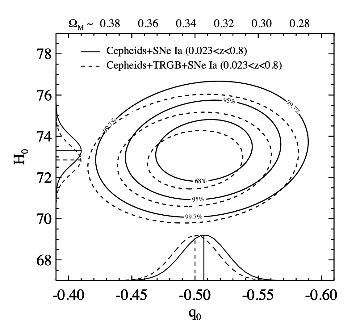
Figure 17: Simultaneous measurement of H₀ and expansion history. Here the expansion history is fit with a single free parameter, $q_{0}$, though as discussed in the text, it can be fit with any form for H$(z)$ using the set of $\mu_{\rm host}$ and a set of consistently standardized SNe Ia in these hosts and in the Hubble flow.

Following this approach, the set of 37 values of $\mu_{0,\textrm{host}}$ for 42 SNe Ia (or 40 values for 46 SNe Ia including the TRGB data as in §6.7) and their covariance matrix, derived from the first two rungs (i.e., without the use of any SN data), are taken as input. The covariance matrix of $\mu_{0,\textrm{host}}$ is shown in Fig. 16. In addition, the values of $m_{B}$ for the SNe in these hosts and in the Hubble flow (including their redshifts) and the covariance matrix between all SN measurements are taken as additional data and the two constraining relations are solved simultaneously.

As an example, in Fig. 17 we follow this approach, marginalizing over the SN standardization parameter, $M_{B}$, and simultaneously measure H₀ and $q_{0}$. As expected, H₀ will be quite uncorrelated with $q_{0}$ (or other cosmological parameters) unless a cosmological model produces a much more rapid change in H$(z)$ at $z\ll 1$ than the polynomial in Equation (17). For this case we add SNe from Pantheon+ at $0.15<z<0.8$ to the prior analysis, finding $q_{0}=$ $-0.51\pm 0.024$ and H${}_{0}=$ $73.30\pm 1.04$ km s^-1 Mpc^-1. The result is very similar to our baseline result and the added freedom in the expansion history has had little impact on the uncertainty. Brout:2022 give results for a Friedman-Robertson-Walker (FRW) expansion history governed by $w$ and $\Omega_{M}$. We provide the SN-independent host distances and their covariance matrix at pantheonplussh0es.github.io to allow for other forms of H$(z)$.

6 Extensions or Variants of the Baseline Analysis

The baseline analysis was identified as providing the most accurate model of the data that is also the most economical in terms of the number of free parameters. Here we review 12 categories of alternatives or extensions to the baseline analysis, selected to explore the sensitivity of the results to additional considerations and systematic uncertainties. These are given as 67 fits listed in Table 5, shown graphically in Fig. 18, and summarized in §6.14.

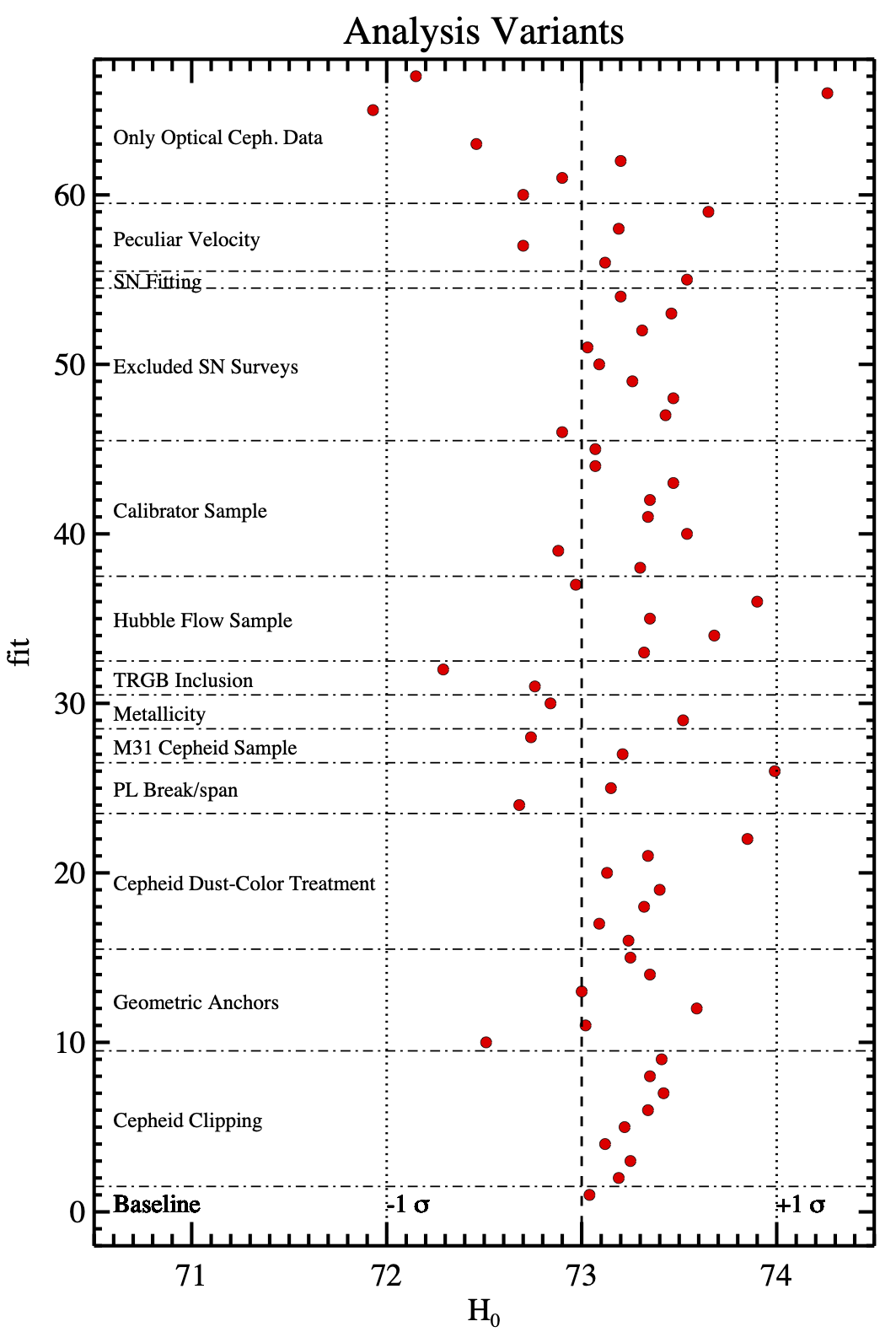
Figure 18: Display of 67 fits in 12 categories of alternatives or extensions to the baseline as shown in Table 5.

6.1 Cepheid Clipping

The optical selection of our Cepheid sample is discussed by H16 and Y22b. As in R16, we include only Cepheids with colors F814W–F160W within 0.8 mag of the median color in each host to remove blends with unresolved sources of comparable luminosity and different color (e.g., red giants, blue supergiants, unresolved star clusters). This is a useful criterion as it is distance- and period-independent, insensitive to reddening, and anchored to the physical properties of Cepheids (i.e., stars with spectral types F–K). We still may expect a small number of outliers owing to fully-blended yellow supergiants, or the sample may include a small number of objects erroneously identified as Cepheids.

Our baseline analysis removes Cepheids that deviate from the global fit at $>3.3\sigma$ (Chauvenet’s criterion), iteratively discarding the single largest outlier (i.e., MAD algorithm) until none remain above the threshold. The fraction of such objects is 1.2% (these outliers are available upon reasonable request). Fits 2–9 explore other rejection approaches: global (i.e., all objects above threshold are removed as opposed to the most deviant followed by recalculation of the fit), from the individual $P$–$L$ relations, and with tighter or looser thresholds ($3\sigma$ or $5\sigma$), as well as no rejection. The median H₀ of these alternatives to the baseline clipping is larger by 0.2 km s^-1 Mpc^-1. Because the global outlier removal (Fit 2) is faster to calculate and gives results within 0.15 km s^-1 Mpc^-1 of the MAD baseline, we use this approach for most other fits unless we explicitly state the use of MAD. For the number of degrees of freedom here, fits with $\chi^{2}_{dof}>1.07$ are considered not good (probability to exceed $>3\sigma$), which applies to Fits 6, 7, and 9 that remove few or no Cepheid outliers.

6.2 Geometric Anchors: Consistency with Metallicity

Fits 10–15 provide the results of including the geometric distance measurement(s) of only one or at most two anchors, rather than all three. The goal here is to explore the possibility of an unexpected error in one of the external geometric distance constraints. In Fig. 19 we compare the geometric distance estimate to each anchor with the value modeled using only its Cepheids and the geometric distance of the other two anchors. As shown, the external measured distances are consistent with their Cepheids at $-0.2\sigma$ for NGC 4258, $+0.4\sigma$ for the LMC, and $-0.5\sigma$ for the MW. Their internal consistency (despite having different mean abundances) is a consequence of the Cepheid metallicity dependence.

The consistency of the anchors is most readily seen by comparing their intercepts and metallicity as shown in Figs. 20 and 21. Here we determine the intercepts from the Cepheid data table for each host, NGC 4258, LMC, SMC, and the MW using their geometric distances for an absolute measure; see also Breuval:2021 for a similar analysis. It is clear that the consistency of the anchors is a direct consequence of the Cepheid metallicity dependence which has been greatly refined since R16. In our primary analysis we find a metallicity dependence on [O/H] of $-0.217\pm 0.046$ mag/dex. In R16 our primary result was $\gamma=-0.13\pm 0.07$ (with variants values ranging from $-0.24$ to $-0.08$) and in R19 it was $-0.17\pm 0.06$. The total $\chi^{2}$ for the three anchors in 21 is 0.18, which for a line fit leaves one remaining degree of freedom, and the likelihood to find agreement this good or better is 33% and thus nominal but not surprising.

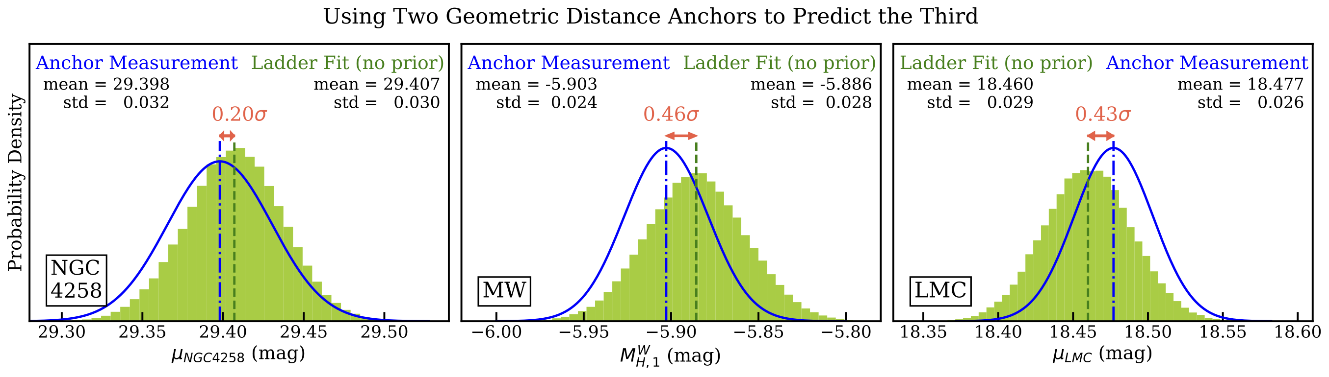
Figure 19: Comparison of each geometric anchor distance with its expected value based only on the Cepheids it hosts and the distance ladder calibrated by the geometric distance of the other two anchors. The green histograms are MCMC samples from Fits 13, 14, and 15 showing the expected distance of an anchor whose independent distance was excluded from the analysis. The independent measurement (blue curve) and prediction (green) are in good agreement in all cases to $<1\sigma$.

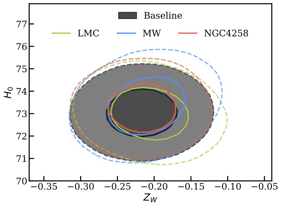
Figure 20: Marginalized posterior covariance between H₀ and the metallicity term, $Z_{W}$, for the three two-anchor cases and the baseline fit. The metallicity term is well-constrained, with a substantial tightening owing to the differential DEB distance between the two clouds (LMC and SMC) from Graczyk:2020. The term has little correlation with H₀ because the anchor abundances span the range in the SN hosts, but this term provides for the consistency between the anchors.

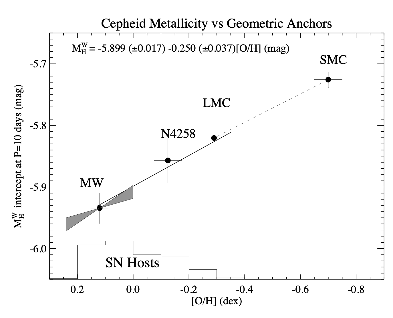
Figure 21: The metallicity term and consistency of the geometric anchors. The mean slope of four hosts with geometric distances is plotted against the intercept of the Wesenheit magnitude $P$–$L$ relation. The DEB distance difference between the SMC and LMC from Graczyk:2020 as discussed is independent of the calibration uncertainties of the DEB method, making this link, the dashed line, robust and independent of the other anchors (a linear fit to the 4 points is very good, though not unexpectedly so with $P=10$% to be better). The gray constraint on the MW comes from the breadth of metallicities and individual Gaia EDR3 parallaxes. The metallicities of the Cepheids in SN hosts span the range of the anchors making the value of H₀ insensitive to the value of the metallicity dependence, with a change in H₀ of 0.2 units for a change in $Z_{W}$ of 0.1 mag dex^-1.

A number of recent developments have tightened this constraint considerably while broadening its range. The DEB distance for the SMC from Graczyk:2020 as discussed in §4.4 provides a differential measurement between the Cepheids in the LMC and SMC which constrains the metallicity dependence. As shown in Fig. 21, this constraint alone gives $\gamma=-0.22\pm 0.05$, similar to the values and uncertainties found by Breuval:2021 for [Fe/H], and falling along the line that joins the other two anchors. It is one of the strongest constraints available because it comes from the difference in the DEB distances to each Cloud, a measure which has small uncertainty owing to calibration cancellation and which does not depend on the comparison between the LMC and the other two anchors (Graczyk:2020). In addition, the constraint internal to the MW Gaia EDR3 parallaxes alone ($-0.22\pm 0.09$) indicates a similar value. The global fit also makes use of the internal metallicity gradients in the SN hosts to constrain $Z_{W}$. Individually, these are not constraining, with a median uncertainty greater than 1 and a minimum of 0.3. However, combined these are supportive of the results from the local galaxies albeit less constraining, yielding $-0.13\pm 0.11$ mag dex^-1 by combining their independent fits with uncertainties in both axes.

Abundance measurements for 68 of the 70 LMC Cepheids used here (Romaniello:2021) show that they are consistent with a single value, and the lack of any measurable breadth in metallicities negates the ability to measure an abundance dependence internal to the LMC as claimed in prior analyses (Freedman:2011) and further discussed by Romaniello:2021. Together, these developments provide a consistent result of a $\sim-0.2$ mag dex^-1 metallicity dependence in the NIR that also provides accord amongst the anchors and is little changed by excluding any anchor as shown in Fig. 20.

It is important to note that excluding knowledge of the geometric distance to an anchor (e.g., the DEB distance to the LMC) as we do in Fits 10–15 does not exclude the Cepheids in that anchor, which remain extremely valuable (at any distance) for constraining the global properties of Cepheids. Rather, when excluding knowledge of an anchor distance, we allow that distance to become a free parameter which may subsequently be compared to the external geometric estimate. In this case a parameter such as the slope of the $P$–$L$ remains constrained by the excluded anchor Cepheids because these Cepheids are only consistent with a single distance to the host with an accurate value of their slope.

6.3 Variants with Color and the Reddening Ratio, $R$

Here we explore variants in how the Cepheid color, $V\!-\!I$, is used in their distance determination. Our baseline analysis derives the Wesenheit parameter $R$ (sometimes refereed to as $R_{H}$ to avoid confusion with the optical reddening law parameter, $R_{V}$) from the Fitzpatrick:1999 law with reddening parameter $R_{V}=3.3$, assuming MW-like reddening for the sample of late-type hosts and thus $R=0.386$. Fits 16, 17, and 18 (respectively) change the reddening parameter to $R_{V}=2.5$ or adopt different laws — cardelli89 or Nataf:2016. The relationship between $R$, $R_{V}$, and the reddening laws is shown in the upper-left panel of Fig. 22. Fit 19 allows the value of $R$ for all hosts to be a common but free parameter. The value derived from MW Cepheids for $R$ is $0.36\pm 0.04$ (Riess:2021) and for the full sample of Cepheids here is $0.34\pm 0.02$. These fits yield a very similar value for H₀; including $R$ as a free parameter has little impact on the uncertainty.

If one wishes to allow for differences in the reddening law or the value of $R$ across different hosts, it is necessary to first subtract the intrinsic color of Cepheids using their empirical period–color ($P$–$C$) relation, in order to separate the component of the color that results from dust reddening; see Appendix LABEL:sc:appd for details. sandage04 dereddened MW Cepheids to determine $\langle(V\!-\!I)_{0}\rangle=0.256\log P+0.497$. We used the LMC reddening maps from Skowron:2021 to deredden the Cepheids in the catalog of Macri:2015 to derive a $P$–$C$ relation of $\langle(V\!-\!I)_{0}\rangle=0.238\log P+0.513$, very similar to the MW one. From the same data we derived the intrinsic $P$–$C$ relation from the LMC Cepheids as above to be $\Delta m_{H}=0.635(\pm 0.021)\ \Delta({V\!-\!I})$.

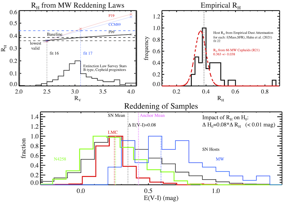
Figure 22: Reddening ratios and impact on H₀. The upper-left panel shows various reddening laws and their free parameter $R_{V}$ used to estimate the appropriate ratio $R_{H}$ for dereddening the Cepheids and the range over which this is applicable. The upper-right panel shows the empirical determination of $R_{H}$ using the MW Cepheids from R21 and individual estimates parameterized by host, type, mass, and SFR from SDSS galaxies in Hahn:2021. The lower panel shows the color excess, $E(V\!-\!I)$, for Cepheid samples. The net change to H₀ due to differential Cepheid reddening on the ladder is 0.08 $R_{H}$ (0.03) mag, with realistic differences in $R_{H}$ producing changes $<0.01$ mag or $<0.5$%.

We use a mean relation of $\langle(V\!-\!I)_{0}\rangle=0.25\log P+0.50$ to first subtract the intrinsic color from all Cepheids using their periods, and then in Fit 20 we substitute the Wesenheit magnitudes in Equation (7) for $m_{H}-R\ E({V\!-\!I})$ with $R=0.386$, which reduces H₀ by 0.1 km s^-1 Mpc^-1. In Fit 21 we allow this reddening ratio to be a free parameter with little change from the result given in Fit 19.

We can also consider different values for the reddening ratio, $R$, for different hosts. One might derive these as the value that optimizes the relation between colors and magnitudes within each host. However, after subtracting the intrinsic $P$–$C$ relation, the small residual color span, coupled with relatively large color measurement uncertainties, does not provide any meaningful constraint on the individual values of $R$ for a given host beyond the few nearest galaxies as demonstrated in Appendix LABEL:sc:appd. In addition, Appendix LABEL:sc:appd shows that determining an unbiased estimate of $R$ requires accounting for uncertainties in both axes (in this case color and brightness with the statistical issue discussed by Tremaine:2002), and failing to do so leads to large underestimates of $R$ and its uncertainty, as seen (for example) in Peri:2021 and Mortsell:2021. We find typical uncertainties in individual values of $R$ to be $\sim 1$, and thus uninformative. Likewise, Follin:2017 also concluded that such color data are “insufficient to make a completely data-driven inference on [individual] $R$,” and they used a “wide-prior” of $0.39\pm 0.1$, finding distant hosts consistent with that prior and little impact on H₀. It is also crucial to recognize that the empirical reddening law is only valid for use at $R_{V}>2.5$, as stated by Fitzpatrick:2019, because sight lines with $R_{V}<2$ are not seen among the hundreds of massive MW stars used to determine the law as shown in Fig. 22 (indeed, the Rayleigh-scattering limit for absorption corresponds to $R_{V}\geq 1.5$). Thus, there is no empirical support for $R<0.3$ from these laws or from the stars (significantly, of the same B-type that later become Cepheids) that inform them.

An alternative approach with better grounding is to derive individual values of $R$ for each host based on its specific properties and the empirically determined correlation of these properties with dust attenuation. We use the empirical dust attenuation (EDA) framework from Hahn:2021, which derives individual extinction laws for hosts as a function of their mass, type, and star-formation rate (SFR) as determined to best match colors to SDSS galaxy observations. These individual estimates of $R$ are given in Table 6 and shown in Fig. 22, and have a mean of 0.42 and dispersion of 0.10, well matching the prior used by Follin:2017. The smallest value for any host is 0.30 for NGC 7541, demonstrating that values lower than this become unrealistic as discussed further in Appendix LABEL:sc:appd. Fit 22 uses these modeled values of $R$ from Hahn:2021 and results in an increase in H₀ of 0.8 km s^-1 Mpc^-1.

It is clear why varying the reddening ratio in hosts is not effective at changing H₀. The mean value of $E(V\!-\!I)$ in the SN hosts is 0.35 mag, as shown in Fig. 22. For the Cepheids in the anchors MW (Gaia EDR3), LMC, and NGC 4258, it is 0.58, 0.23, and 0.24 mag (respectively), for a mean anchor value (weighted by the precision of the anchor distance) of 0.43 mag. Thus, the net difference in $E(V\!-\!I)$ between anchors and SN hosts is 0.08 mag, and hence the full impact on H₀ of correcting for Cepheid reddening is 0.03 mag or $\sim 1.5\%$, with perturbations to this procedure changing the result by a smaller amount. As shown in Fig. 22, the strongest empirical evidence has the characteristic value of $R$ less than 0.1 from the baseline; hence, e.g., $\Delta$H${}_{0}=0.08\Delta R$ (mag) $<0.01$ mag. In Fit 23 we discard the use of color altogether, representing a reasonable assumption that the Cepheid extinction at 1.6 $\mu$m is modest and to first approximation cancels along the distance ladder, and find that H₀ goes up by 2%.

6.4 Form of the P–L Relation

In §4.6 and Fig. 10 we measure the slopes of the $P$–$L$ relations of each host as well as the mean slope above and below $P\!=\!10$ d, finding no clear evidence of a break. It is important to note that we have not included Cepheids with $P\!<\!5$ d (either in the anchors or SN hosts) in our analyses. Such Cepheids could provide additional support for a break; however, Cepheids with overtone pulsations become much more common below this period, obey a different $P$–$L$ relation, and may be confused with fundamental Cepheids.

However, in R16 the baseline was to allow for a break at $P=10$ d, in accord with prior claims of a break in the optical in the LMC (sandage04, although no evidence for one was found by R16). To allow for additional comparison to R16, in Fit 24 we allow for a break at $P\!=\!10$ d with independent slopes above and below this pivot. The two slopes have a slope difference of $0.10\pm 0.05$ as given in Table 5 which lowers H₀ by 0.45 km s^-1 Mpc^-1, with the difference largely driven by the ground-based samples from the LMC and SMC, whose Cepheids at lower periods have a shallower slope by $0.12\pm 0.08$ and $0.34\pm 0.20$ (respectively). To further explore the evidence for a break, we expand the sample of Cepheids in M31 by including those from Kodric:2018 in Fit 28. Because in M31 the opposite occurs (shorter-period Cepheids have a steeper slope by $0.20\pm 0.12$), the inclusion of both samples reduces a difference in slope to $0.07\pm 0.04$ and H₀ lower than the baseline by only 0.3 km s^-1 Mpc^-1. A free-form analysis of a slope change (allowing each host to have two individual slopes) reduces the sample evidence of a break to $<1\sigma$, with only three hosts (the LMC, SMC, and M31) providing any significant weight at $P<10$ d (MW Cepheids with Gaia parallaxes provide no indication of a change in slope). The lack of significant evidence of a break (or change in slope) is why the baseline analysis uses the single-slope parameterization. Another option here is to exclude Cepheids with $P<10$ d which we do in Fit 25, resulting in an 0.1 unit increase in H₀.

6.5 M31 Variants

Fits 27 and 28 exchange the Li:2021 sample of M31 Cepheids for the PHAT sample from Kodric:2018 with a ten-fold increase in the number of variables, but with filters that are transformed to the set of three used elsewhere rather than directly observed with them. The main value of this change is to gain further traction of a possible break at $P\!=\!10$ d as discussed in the prior section.

6.6 Variants of Metallicity

In Fit 29 we neglect the metallicity term and find that it has little impact, with H₀ rising by 0.3 km s^-1 Mpc^-1. The metallicity term has little impact on H₀, as shown in the marginal confidence region of Fig. 20. The reason can be seen in Fig. 21, where the distribution of Cepheid metallicities in SN hosts well matches the range of the three anchors; thus, the metallicity term does not move the SN hosts with respect to the mean of the anchors. It does, however, provide for consistency of the Cepheid and anchor distances.

Appendix LABEL:sc:appc gives further details about the Cepheid metallicity scale we adopt, the average of nine recent and well-characterized relations (Teimoorinia:2021). In Fit 30, we replace the use of the mean metallicity scale with one of these systems (Pettini:2004) based on [O III] and [N II] lines, which we show in Appendix LABEL:sc:appc provides consistent metallicities for MW H II regions with those at the same radius derived from spectra of MW Cepheids.

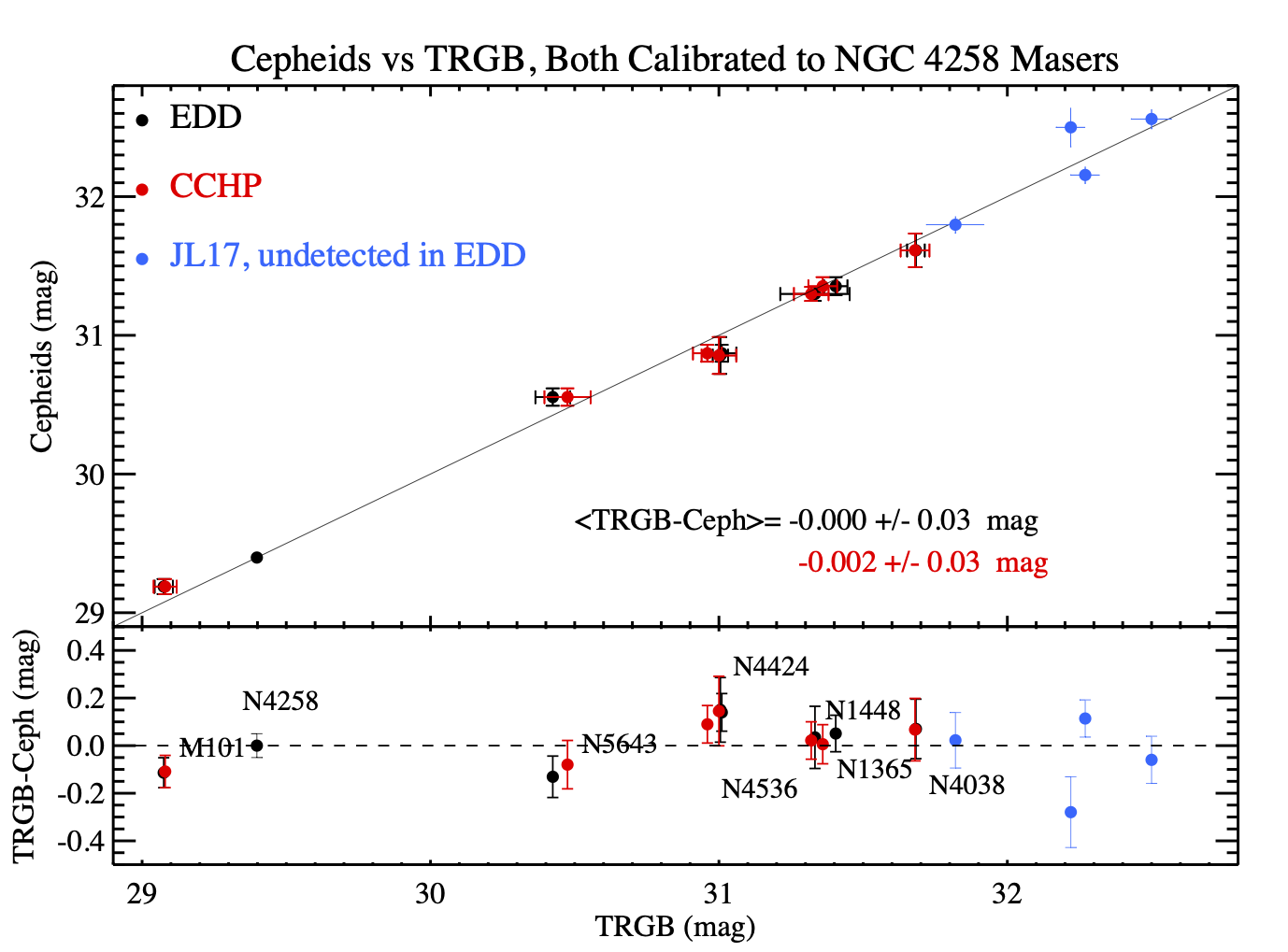
Figure 23: Cepheid distances from this work and TRGB distances from the CCHP (F21) and the EDD (Anand:2021) groups to the same SN hosts calibrated by the same geometric anchor distance to NGC 4258, all measured with HST. The seven hosts indicated are all of those measured by these three groups. In blue we show four more-distant hosts measured by Jang:2017 for which evidence of a TRGB was not detected by Anand:2021. The Cepheid and TRGB distances are consistent, allowing us to combine them (including for three additional TRGB hosts: NGC 1316, 1404, and 4526) simultaneously in Fits 31 and 32.

6.7 Inclusion of TRGB

The TRGB offers an additional, independent rung between anchors and SN hosts (Freedman:2019; Anand:2021, and references therein). The inclusion of TRGB distances can in principle improve the calibration of SN Ia hosts and add to the number of such objects on the second rung. However, before including TRGB distances, it is important to determine if they are consistent with those employed here for Cepheids. We use the TRGB samples measured by the CCHP (Freedman:2021) and EDD (Anand:2021) groups.

To determine the consistency of the two distance indicators, we calibrate both using the same geometric anchor, NGC 4258, whose Cepheids and TRGB were both observed with HST, making this a purely differential comparison to a set of the same SN hosts. In Fig. 23 we compare the distances from each method for all seven SN Ia hosts with Cepheid and TRGB measurements which are available from both CCHP and EDD. The mean difference between Cepheids and TRGB is $0.000\pm 0.030$ and $0.002\pm 0.030$ mag for EDD and CCHP, respectively (we have not included the four more-distant SN Ia hosts measured by Jang:2017 and included in F19 because Anand:2021 could not identify any reliable TRGB for these, but we plot them in Fig. 23), and conclude these are consistent (see §7.2 for further discussion). For consistency with the preceding Cepheid-only analyses, we do not include SNe Ia with TRGB measures which do not pass the SN quality cuts employed above ($\mathinner{\!\left\lvert c\right\rvert}<0.15$ and $\mathinner{\!\left\lvert x1\right\rvert}<2$), which affects four objects (SNe 1989B and 1998bu with $c=0.3$ corresponding to $A_{V}\approx 1$ mag, and SN 1981D with $c=0.2$, also with high reddening; SN 2007on with $x1=-2.2$). Ten TRGB distances for 11 SNe Ia are thus added: the seven hosts with Cepheid distances (and eight SNe) in Fig. 23 (M101, NGC 1365, 1448, 4038, 4424, 4536, 5643) and three additional hosts without Cepheids with four additional SN calibrators (SNe 1980N and 2006dd in NGC 1316, SN 2011iv in NGC 1404, and SN 1994D in NGC 4526).

As we did for the Cepheids, we use TRGB distances where the anchor and SN hosts made use of the same telescope and instrument to negate telescope zeropoints. In this case we first use Table 2 from Anand:2021, which includes the calibration based on new observations of NGC 4258 from our program (GO 16198) that also employ the same filters (F606W & F814W), ACS electronics and similar level of CTE as for the SN hosts. We do not include TRGB zeropoints in the Magellanic Clouds or the MW because these have not been measured directly on the HST system (owing to the impracticable area). For the joint analysis we include an additional parameter for the TRGB luminosity, $M_{I}$, which is optimized in the fit. We note that the TRGB constraint is included as available for a SN host simultaneously with the Cepheid constraint through the addition of the relation for the $i$-th SN host,

$$m_{I,\textrm{TRGB},i}=\mu_{0,i}+M_{I,\textrm{TRGB}},$$ (20)

and the calibrating relation

$$m_{I,\textsc{n4258}}-\mu_{0,\textsc{n4258}}=\Delta\mu_{\textsc{n4258}}+M_{I,\textrm{TRGB}},$$ (21)

which adds a single free parameter, $M_{I,\textrm{TRGB}}$.

Including TRGB (EDD), Fit 31 lowers H₀ by 0.3 units to $72.76\pm 0.95$ km s^-1 Mpc^-1 and reduces the overall error by 5%, yielding a value of $M_{I}=-4.003\pm 0.025$ mag similar to that found by Anand:2021. The TRGB SN host and Pantheon SN data yield 71.5 km s^-1 Mpc^-1 before the sample is tripled by combining with the SN-Cepheid hosts with the increase in H₀ of $\sim 1$ km s^-1 Mpc^-1, consistent with the shot noise of each subsample as discussed in detail in §7.2. We note that because the EDD TRGB parameterization includes a color dependence, the value of $M_{I,\rm{TRGB}}$ quoted here corresponds to their fiducial, blue TRGB with $V\!-\!I=1.23$ mag. For Fit 32 we replace the EDD TRGB measurements with the CCHP set as given by F19 and F21 for the same SN hosts and by Jang:2021 for NGC 4258 TRGB and without a color dependence to match the CCHP implementation. This reduces H₀ by 0.45 units from the EDD-based result (0.75 units below the baseline). The difference between the EDD and CCHP-based result is a direct consequence of the 0.04 mag brighter measurement of the tip in NGC 4258 by Jang:2021 compared to EDD, the significance of which is $1.9\sigma$ as further discussed in §7.2. The Jang:2021 measurement in NGC 4258 in concert with the other constraints yields $M_{I,\rm{TRGB}}=-4.025\pm 0.023$ mag for the above parameter. (We note that a direct comparison of the $M_{I,\rm{TRGB}}$ parameter to that observed for NGC 4258 requires adding to this $\Delta\mu_{\rm N4258}$ in Equation (2), which for the baseline is $-0.013$ mag.) The mean result from the two TRGB implementations is $72.53\pm 0.95$ km s^-1 Mpc^-1, which we adopt as a reference value for TRGB inclusion.

6.8 Hubble-Flow SN Sample Variants

Here we explore fits utilizing different selection criteria for inclusion in the Hubble-flow sample. The goal of the selection of SNe and their hosts for the Hubble-flow sample is to match as well as possible the same criteria used to collect the calibrator sample to guard against the presence and imbalance between samples of additional host or SN characteristics currently known or unknown that may correlate with Hubble residuals. The enhanced size of the calibrator sample, now with 42 SNe Ia, reduces the likelihood of a chance imbalance of such properties.

The host selection for the baseline Hubble-flow samples requires visual identification from the best available optical imaging to be a spiral type in the full range of Sa–Sd, making them likely hosts of massive star formation in the last 0.1 Gyr — the primary criterion for our targeting them for Cepheid observations. This excludes highly-inclined hosts ($>75^{\circ}$) as these are complex targets and were not considered for finding Cepheids nearby. The host requirements are in addition to the SN Ia quality cuts which are relatively tight in order to match the calibrators ($\mathinner{\!\left\lvert c\right\rvert}\leq 0.15$, $\mathinner{\!\left\lvert x1\right\rvert}<2$), with the first observation earlier than 5 d after maximum light, distance measurement error of $\leq 0.2$ mag, with outliers $>3.5\sigma$ from the Hubble flow removed. The redshift range, as in R16, is $0.0233<z<0.15$. We refer to this sample as “LZSPI” (low-$z$, spiral). In §7.2 we will further analyze the host properties of these samples to confirm their balance in mass, SFR, and specific star-formation rate. In Appendix A we compare the colors and light-curve shapes of the SN samples, confirming the similarity of the calibrator and selected Hubble-flow sample.

In Fit 33 we expand the Hubble-flow sample by removing any limitation on the host and including all SNe that pass the Pantheon+ quality cuts (which allow $\mathinner{\!\left\lvert c\right\rvert}\leq 0.3$ and $\mathinner{\!\left\lvert x1\right\rvert}<3$), nearly doubling the sample to 482 SNe. It is noteworthy that there is no change in H₀, suggesting that after Pantheon+ standardization, SNe in different host types provide consistent distances. In Fit 34, we expand the sample to high redshift ($z<0.8$) and more than 1300 SNe, which raises H₀ by 0.5 km s^-1 Mpc^-1. The use of such high-redshift SNe requires knowledge of $q_{0}$ as discussed in §5.2 and §6.12. Fits 35 and 36 use these two expanded samples but exclude $z<0.06$ to circumvent concerns about the presence of a hypothesized local void structure. These raise H₀ by $\sim 0.3$ km s^-1 Mpc^-1.

6.9 Calibrator SN Sample Variants

Here we explore variations of the calibrator sample. A complete, volume-limited sample is desirable, as it has the simplest and most unbiased selection function. Such a sample is limited by the volume $z\leq 0.011$ of suitable calibrators between 1980 and 2021 and can be selected by excluding two SNe Ia from the baseline sample at higher redshifts (SNe 1999dq and 2007A), with results given in Fit 38. Fit 39 contains the same with the added TRGB distance measures. Fit 40 limits the hosts to only high-mass galaxies, $\log\,(M/M_{\odot})>10$.

In §7 we discuss tests of the Cepheid background. Here we undertake another test of the background with Fits 41 and 42, which divide the calibrator sample into halves with lower-than and higher-than median background. The difference in H₀ is 0.0 km s^-1 Mpc^-1, which is much less than the independent shot noise of each half (1.3% or 0.9 units for each), and thus there is no indication of a difference in H₀ for high and low backgrounds. Fits 43 and 44 respectively use only the same 19 SNe from R16 or only the 23 SNe Ia added here, yielding a difference of 0.4 units. Fit 45 includes only the nearer half, defined as having $m_{B}<13$ mag (the median of the sample, corresponding to $D<28$ Mpc), as nearer hosts offer greater spatial resolution, lowering H₀ by 0.1 units.

6.10 Excluded SN Survey Variants

The SN standardized magnitudes have been drawn from the Pantheon+ sample, which is based on more than a dozen past SN surveys. The Pantheon+ sample recalibrates each survey photometrically to a common reference using the standard-star measurements in the fields of each SN to negate the impact of survey calibration errors. In addition, most SNe observed in the Cepheid host sample are matched by SNe in the Hubble-flow sample observed by the same SN survey with no one survey having a dominant share. As demonstrated by Brownsberger:2021, “gray” photometric survey errors strongly and beneficially cancel by populating both samples with SNe from the same surveys. Brownsberger:2021 find that survey miscalibration and incomplete cancellation would affect H₀ measured from the survey mix used here at $\sigma=0.15$ km s^-1 Mpc^-1 even for extremely large survey zeropoint errors of $\sim 0.1$ mag, and more likely 0.06 units for realistic survey calibration errors of 0.025 mag.

To further explore the sensitivity of H₀ to survey errors, Fits 46–54 present the results excluding each of the major surveys contributing to the sample. While none of these exclusions change the baseline H₀ by more than $\sim 0.3$ units, we note that excluding the CSP sample raises H₀ by 0.3 units, with most of this (0.2) seen in the change in the Hubble intercept ($a_{B}$). Using a Hubble-flow sample exclusively from the CSP (while using a mix of surveys for the calibrator sample) yields a lower value of H₀ by 0.5 units. While this is consistent with the sample shot noise, it will reduce H₀ for the CCHP results which use only the CSP sample for the Hubble flow. Brownsberger:2021 find that this sample asymmetry is expected to produce errors of 0.8 units for realistic calibration errors of 0.025 mag; it is discussed further in §7.2.

6.11 SN Fitting Variants

Fit 55 changes the way the intrinsic scatter of SN colors is modeled from an empirical approach that includes both a component intrinsic to SNe Ia and another due to host dust as given by Brout:2021, and is further described in the Pantheon+ sample (Brout:2022; Scolnic:2021). It is a simpler description, where the intrinsic scatter of SNe Ia is monochromatic (i.e., dispersion only in the luminosity, not the color) from Guy:2010 and used in the JLA analysis (Betoule:2014) and in the first Pantheon compilation (Scolnic:2018). This fit raises H₀ by 0.3 units. The calibrator sample has no preference for either method, yielding similar dispersion between SN and Cepheid distances.

6.12 Velocity Variants

Here we provide variations related to values of the redshifts as implemented in Equation (4), which benefit from the combined and improved values from Pantheon+ (Carr:2021). Peterson:2021 provide a comprehensive overview and comparative analyses of various predictions of empirical cosmic flows (or peculiar velocities). They found important improvements to the Hubble-flow residuals by (1) replacing SN host redshifts with their host-galaxy group redshift (when available), and (2) using local density maps to account for motions induced by local gravity. The latter are provided by constrained realizations of the peculiar-velocity field by Carrick:2015 and Lilow:2021 based on 2M++ (Lavaux:2011) and 2MRS (Huchra:2012; Macri:2019), respectively. The baseline included both the group-redshift replacement and the 2M++ corrections from Peterson:2021. Fit 56 exchanges the 2M++ values for those from 2MRS, which provide a comparable improvement in residuals and lower H₀ by 0.05 units. A noteworthy change is seen in Fit 57, which forgoes the flow corrections and leaves the redshifts in the CMB frame, reducing H₀ by 0.5 units. However, as shown by Peterson:2021 for 585 SNe Ia with $z<0.08$, the tightening of the Hubble diagram (from $\sigma=0.17$ mag to $<0.15$ mag, or a decrease in $\chi^{2}$ of 100) gives evidence in favor of these corrections which is too strong to neglect. Further, the increase in H₀ that comes with the decrease in residuals runs counter to the hypothesis that the SN sample lives inside a large-scale void that artificially raises the local value of H₀ (Kenworthy:2019).

While peculiar flows cause a small perturbation in H₀ measured from SNe Ia at $0.0233<z<0.15$, they would produce a greater uncertainty if we forgo the use of SNe and measure H₀ directly from only the first two rungs — that is, from the Cepheid host redshifts (which are not used in the three-rung distance ladder). The baseline sample host redshifts have a mean of $cz=2000$ km s^-1, with many $<1000$ km s^-1. Elsewhere (Kenworthy et al. 2022, in prep.), we present an analysis of H₀ from this two-rung ladder which importantly accounts for the spatial covariance of the local peculiar flows, largely limiting the available precision from this route to 3%–4% and demonstrating the value of SNe Ia for the third rung for measuring H₀.

Fits 58 and 59 raise $q_{0}$ from $-0.55$ to $-0.52$ (equivalent to raising $\Omega_{M}$ in flat $\Lambda$CDM from 0.30 to 0.32) for either the local sample of spiral hosts or the sample with all hosts and for $z<0.8$, with little impact on H₀ relative to these samples at $q_{0}=-0.55$. In §5 we considered a free-form fit for H$(z)$ using $q_{0}$ as a free parameter simultaneous to the determination of H₀.

6.13 Optical Wesenheit Variants

Fits 60–67 use an optical-only Wesenheit magnitude, substituting for Equation (7), $m^{W}_{I}=m_{I}-R(V\!-\!I)$, and thus discarding the NIR observations. The Fitzpatrick:1999 reddening law with $R_{V}=3.3$ yields $R=1.19$ in the HST passband system ($m_{V}$ = F555W, $m_{I}$ = F814W). The optical Wesenheit has the advantage of lower “sky” backgrounds (and their fluctuations) but the disadvantage of higher reddening (and sensitivity to the form of the reddening law). The baseline fit with the optical Wesenheit yields $72.70\pm 1.07$ km s^-1 Mpc^-1, similar to the baseline fit. However, the optical Wesenheit is somewhat noisier when compared to the SN distances with a relative dispersion of 0.16 mag (vs. $\sim 0.13$ mag with the NIR data). We also see larger variations in the anchors and the color variants as seen in Fig. 18, with the scatter among optical-based variants that is three times greater than the NIR-based results and comparable to the statistical uncertainties. This illustrates the rationale by the SH0ES program for pursuing NIR observations for Cepheids.

Both of these differences are expected consequences of variations in the reddening law in the optical. For example, for hosts whose Cepheids have a mean $E(V\!-\!I)=0.4$ mag, a difference between a Fitzpatrick:1999 reddening law with $R_{V}=2.5$ and $R_{V}=3.3$ causes a difference in distance of only 0.01 mag for the NIR Wesenheit but 0.09 mag for the optical one, which can explain the aforementioned noise. In R16 we concluded that future improvements must rely on NIR data until additional studies of variations in reddening laws in the optical were available. The situation has not improved in that regard. While optical-only Wesenheit data have yielded similar values of H₀ (freedman12; Riess:2016), their larger systematic uncertainties make them unsuitable to pursue the percent-level determination of H₀ we approach, and their further analysis is not pursued here. Nevertheless, none of the optical Wesenheit fits result in a noteworthy change to H₀.

Table 7: H₀ Error Budgets (%), terms approximated from global fit

Term	Description	Riess+ (2016)			Riess+ (2019)			This work
		LMC	MW	4258	LMC	MW	4258	LMC	MW	4258
$\sigma_{\mu,\rm anchor}$	Anchor distance	2.1	2.1	2.6	1.2	1.5	2.6	1.2	1.0a	1.5b
$\sigma_{{\rm PL,anchor}}$	Mean of $P$–$L$ in anchor	0.1	$\dots$	1.5	0.4	$\dots$	1.5	0.4	$\dots$	1.0
$R\sigma_{\lambda,1,2}$	zeropoints, anchor-to-hosts	1.4	1.4	0.0	0.1	0.7	0.0	0.1	0.1a	0.0
$\sigma_{Z}$	Cepheid metallicity, anchor-hosts	0.8	0.2	0.2	0.9	0.2	0.2	0.5	0.15	0.15
	subtotal per anchor	2.6	2.5	3.0	1.5	1.7	3.0	1.4	1.0	1.8
		$\underbrace{\hskip 71.13188pt}$			$\underbrace{\hskip 71.13188pt}$			$\underbrace{\hskip 76.82234pt}$
All Anchor subtotal			1.6			1.0			0.7
$\sigma_{{\rm PL}}/\sqrt{n}$	Mean of $P$–$L$ in SN Ia hosts		0.4			0.4			0.4
$\sigma_{\rm SN}/\sqrt{n}$	Mean of SN Ia calibrators (# SN)	1.3 (19)			1.3 (19)			0.9 (42-46)
$\sigma_{m-z}$	SN Ia $m$–$z$ relation		0.4			0.4			0.4
$\sigma_{\rm PL}$	$P$–$L$ slope, $\Delta$log $P$, anchor-hosts		0.6			0.3			0.3
statistical error, $\sigma_{{\rm H}_{0}}$			2.2			1.8			1.3
Analysis systematicsc			0.8			0.6			0.3
Total uncertainty on $\sigma_{{\rm H}_{0}}$ [%]			2.4			1.9			1.35

Note. — ^aRiess:2021. ^bReid:2019. ^cUncertainties labeled in past analyses as “systematics” related to the metallicity scale, Cepheid background/crowding corrections, and SN systematics are formally included here in the covariance matrix in Fig. 11 and thus propagate there as part of the complete uncertainty. Following past work, we measure the remaining systematic errors as the standard deviation of analysis variants presented in each work as in the dispersion in Fig. 18 and as discussed in §6.14. All terms here are approximations derived from the global fit.

6.14 Summary of Variants and Error Budget

Our baseline determination of H₀ lies 0.2 km s^-1 Mpc^-1 (20% of the uncertainty) below the median of all analysis variants, indicating that it is a good proxy for the set. In R16 we measured the dispersion of 23 variants and identified that as a systematic error. In this analysis we have moved previous sources of systematic uncertainty into the covariance matrix to include them formally, and thus most of the variants presented here were intended to gauge sensitivities in the analysis (e.g., excluding a data source) rather than true uncertainties. Nevertheless, we measure the dispersion of the NIR variants (see Fig. 18) around a $3\sigma$-clipped mean to be 0.3 km s^-1 Mpc^-1 and conservatively add this in quadrature as characterizing additional systematic uncertainties to yield a full uncertainty in H₀ of 1.04 km s^-1 Mpc^-1, or 1.4%.

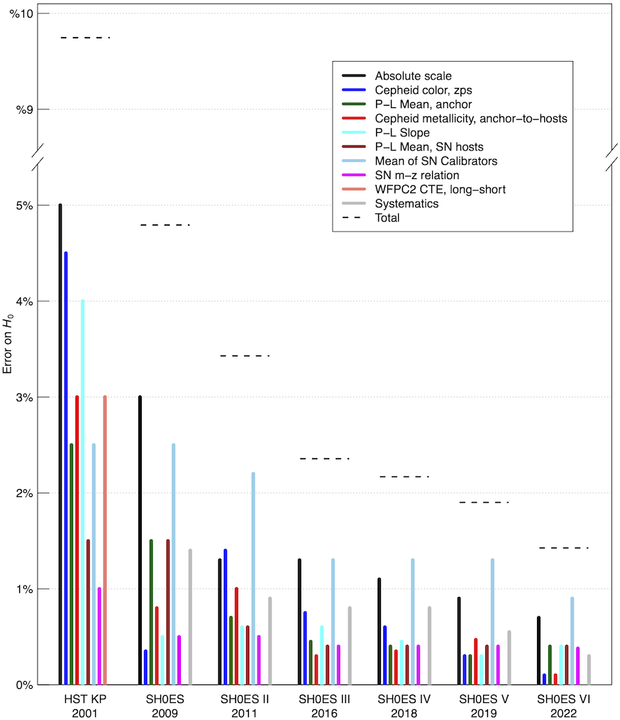
Figure 24: Comprehensive error budgets for six iterations of the SH0ES measurement of H₀ including this one (2022) and the Key Project from 2001 (freedman01). The greatest improvement here is realized by the increase in the number of SN calibrators, to decrease all terms to $<1$%. The combined error is indicated by horizontal dashed lines.

None of the variants appear to offer a particularly promising route to solving the Hubble tension, with none shifting the value of H₀ much below the full error interval. The lowest value of H₀ comes from Fit 65, $71.93\pm 1.19$ km s^-1 Mpc^-1, from discarding the NIR Cepheid data and two anchors (leaving only the Milky Way); the highest is from Fit 22, $74.85\pm 2.33$ km s^-1 Mpc^-1, and comes from discarding the use of Cepheid colors to account for extinction. Both of these fits represent suboptimal accounting of dust.

Table 7 and Fig. 24 present the full error budget derived (in approximate form) from the global fit and in comparison to prior analyses from the SH0ES team. The fractional reduction presented here is the largest seen since between riess11 and Riess:2016.

7 Discussion

Here we address a number of considerations using the preceding fits.

7.1 Accuracy of Cepheid Photometry

The accuracy of Cepheid photometry is important to the measurement of H₀. The dependence of photometry on calibration has been negated by the use of the same photometric system throughout the above measurements. Here we review a number of tests of the relative accuracy for extragalactic Cepheids.

1. Replication of PSF photometry by others: Measurements of NIR PSF Cepheid photometry using the same raw pixels but different software and methods have been directly compared to those used here by Javanmardi:2021 in NGC 5584 and by Yuan:2021_N4051 in NGC 4051, both finding good agreement with reported differences in distance moduli of $0.024\pm 0.046$ and $0.00\pm 0.04$ mag (respectively). While this is short of a full replication of all hosts, it is sufficient to exclude a large methodological error in Cepheid photometry as a primary source of the $\sim 0.2$ mag H₀ tension.

2. Replication of PSF photometry with apertures: In Appendix B we use aperture photometry, an independent method which is simple, highly reproducible, and accurate, albeit less precise than the standard approach of using PSFs to model photometry in crowded fields. For this validation we employ aperture photometry for which the background is measured from the mean pixel value (not the mode of the background pixels) in an annulus centered on the Cepheids. This approach does depend on artificial-star measurements to determine the variable background because the pixels in the annulus include the mean source contribution to the background. We compare the photometry and find good agreement in their means with a difference (PSF minus aperture) of $0.008\pm 0.010$ mag for the Cepheids in SN Ia hosts and $0.002\pm 0.030$ mag for the Cepheids in NGC 4258.

There are a number of strong tests of the accuracy of background estimates presented here.

1. The Cepheids in NGC 4258 have a similar mean level of crowded backgrounds as in the SN Ia hosts (see Fig. LABEL:fg:vscrowd), almost fully negating a systematic underestimate or overestimate of the background on the determination of H₀ when NGC 4258 is the sole anchor. The crowded background is similar because although NGC 4258 is 3–4 times closer than the mean SN host, its Cepheids have been mined from fields which are closer to the dense center by a similar factor. This results in H₀ = $72.51\pm 1.54$ km s^-1 Mpc^-1, similar to the baseline result.

2. In Fig. 8 we compare the $P$–$L$ relations of Cepheids in the dense, inner (high background) and sparse, outer region (low background) of NGC 4258, finding a negligible difference of 0.01 mag.

3. In Appendix B we regress the background with the distance-ladder fit residuals and find a dependence of $0.010\pm 0.014$ mag per magnitude of source background (in the sense of overestimating the background, and consistent with no misestimate). The background misestimate trends required to explain the tension are strongly excluded as shown in Fig. LABEL:fg:vscrowd.

4. The optical background is nearly an order of magnitude smaller than in the NIR owing to the higher resolution, smaller pixels, and lower flux from red giants. The baseline results are consistent with those from the optical Wesenheit which do not include the NIR data, H₀ = $72.70\pm 1.30$ km s^-1 Mpc^-1.

5. There is no significant trend with distance and distance difference between Cepheids and SNe Ia (zero at $<1.5\sigma$); see Figs. 12 and 13.

6. Splitting the calibrator sample by background (Fits 41 and 42) yields no difference in H₀. Splitting in distance (determined by the SN Ia, Fit 45) yields a difference of 0.1 units. Both are consistent with no trend based on the shot noise of half the sample (1.0 units).

Finally, external to this paper, an additional and unavoidable consequence of the miscalibration of the background, independent of Cepheid mean flux, would be a change in apparent light-curve amplitude. Riess:2020 compared the NIR amplitudes of Cepheids in SN hosts and in the MW, found them to be consistent, and provided a quantitative limit of any misestimate of background to be 0.03 mag.

7.2 Consistency of TRGB and Cepheid Distance Scales

In Fig. 23 we presented a comparison of distances measured with Cepheids and TRGB to seven SN Ia hosts — the set that allows for a purely differential and direct comparison by employing the same geometric calibration source (NGC 4258), with data in both host and calibrator obtained with the same telescope (HST) and setup to negate zeropoint and geometric calibration errors. This comparison further employed the two most widely-used methods for measuring the TRGB, edge-detection (F19) and luminosity-function fit (EDD). These Cepheids and TRGB measures are consistent with each other, with a mean difference of $-0.002\pm 0.03$ mag (CCHP; Freedman:2021) and $0.000\pm 0.03$ mag (EDD; Anand:2021). With no mean difference between methods as a starting point, we explore the broader question of the sources of difference in the value of H₀ from distance ladders measured through the use of either method.

In Table 8 we expand on the results from Anand:2021, who compared the value of H₀ from EDD, $71.5$ km s^-1 Mpc^-1, and CCHP, $69.8$ km s^-1 Mpc^-1, derived using the same images to measure the TRGB and the same geometric calibration source, NGC 4258. For consistency with the comparison presented by Anand:2021 of EDD and CCHP which was provided in the units of magnitudes (for differences in $5\,\log\,\Delta$H₀) we retain this unit below and in Table 8 in which a difference of 0.03 mag corresponds to a difference of $\sim 1.0$ km s^-1 Mpc^-1.

The largest contribution (0.04 mag of the full 0.05 mag difference) arises from the difference in the calibration of TRGB measured in NGC 4258 applicable (i.e., in relation to) the mean SN host, where CCHP derive $M_{I,\textrm{TRGB}}=-4.05$ mag for a blue TRGB and EDD derive $M_{I,\textrm{TRGB}}=-4.01$ mag, color-corrected to the fiducial, blue TRGB with F606W$-$F814W = 1.2 mag. Although additional sources in the LMC and MW have been used to support the TRGB calibration by F21, we use NGC 4258 as the reference here because it is the only source where the TRGB calibration is available directly on the HST system measured in a manner consistent with the TRGB in SN hosts. The difference in the EDD and CCHP measurement of the tip in NGC 4258 is persistent, having been found for two different fields of NGC 4258 being significant at the $\sim 2\sigma$ level and is readily evident in Fig. 3 of Anand:2021, where the apparent location of the TRGB edge of $m_{\rm F814W}=25.372\pm 0.014$ mag given by Jang:2021 appears much brighter than the edge highlighted at $25.43\pm 0.025$ mag. A comparison of each group’s color-magnitude diagrams (i.e., photometry) might identify the cause of the difference, but these data are only available from Anand:2021. Nevertheless, we offer the option for either TRGB result in Fits 31 and 32.

The second half of Table 8 provides the sources of difference between the EDD TRGB analysis (based on 16 SNe Ia) for which H${}_{0}=71.5$ km s^-1 Mpc^-1 and our baseline analysis with TRGB (based on 46 SNe Ia), starting with the same geometric calibrator (NGC 4258). The primary change is in the makeup of the Cepheid and TRGB study calibrator samples with 34 SNe Ia added here and 4 subtracted, a net change of 30 objects producing a net increase in H₀ of 0.03 mag or 1 km s^-1 Mpc^-1. The first three rows break out changes related to calibrators available from both TRGB analyses which together lower H₀ by 0.03 mag. The first change is due to the addition of SN 2021pit which recently appeared in NGC 1448 and is added here. SN 2007on has a light-curve shape ($x1=-2.2$) which falls outside the quality range of $|x1|<2$ imposed in our baseline analysis and is excluded. There are three SNe Ia (SNe 1981D, 1989B, and 1998bu) used by CCHP and EDD that are redder ($c>0.15$ and $A_{V}>0.5$ mag) than our baseline quality range cut and have not been included in this or any past SH0ES analyses. The next row adds 33 SNe Ia in 30 Cepheid hosts, tripling the sample from the preceding line’s 13 SNe Ia in 10 hosts (with EDD and CCHP TRGB measurements and not excluded by SN quality cuts) to 46 SNe Ia in 40 hosts (for Fit 30, which includes TRGB-only hosts). This step raises H₀ by 0.06 mag or 2 km s^-1 Mpc^-1. This difference is fully seen internal to the set of Cepheid-only SN Ia calibrations (i.e., independent of absolute anchors or TRGB distances) in the baseline fit as shown in Fig. 25, which compares the two sets of SNe as measured only by Cepheids. The 9 SNe in 7 EDD TRGB hosts are brighter than the 33 SNe Ia in 30 hosts without EDD and CCHP TRGB by $0.08\pm 0.05$ mag as measured by Cepheids, which is consistent at $1.6\sigma$ with the sampling noise of the two sets (0.04 mag and 0.02 mag random error, respectively). As seen in Fits 38–45, this difference does not correlate with potentially relevant changes to the calibrator sample including splitting in distance, background level, or newness of the measurements, so we conclude that this difference of $1.6\sigma$ is a not-unexpected result of the increase in sample statistics.

Combining all of the additions and subtractions to the calibrator sample, the net change between the calibrator samples with both TRGB measures versus the baseline+TRGB here is 0.03 mag and the combined result of all membership changes is less than $1\sigma$ from the shot noise of the two samples. We note that if we use only the (average) TRGB results of the 13 good-quality SNe, discarding 33 good-quality SNe with only Cepheid measurements, we get $71.0\pm 2.5$ km s^-1 Mpc^-1 as expected (near the mean of CCHP and EDD), but this uses less than a third of the SN sample and has higher shot noise, while still consistent with the baseline.

As the sample size from both methods increases, we would expect them to regress to an increasingly similar mean. Including the two other anchors (MW and LMC) raises H₀ by 0.02 mag (and results in $M_{I,\textrm{TRGB}}=-4.00\pm 0.024$ mag), though each of the three anchors is consistent with the others at the $0.5\sigma$ level, as shown in Fig. 19.

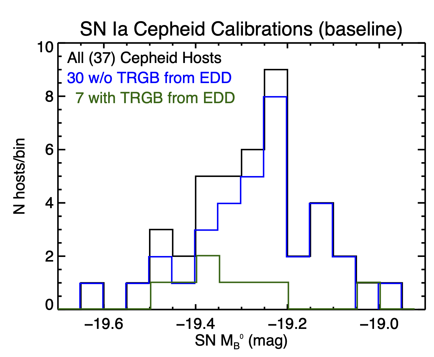
Figure 25: Histogram of the 42 SN Ia absolute magnitudes of SNe Ia calibrated from Cepheids in 37 hosts. The 9 SNe Ia in 7 hosts for which a TRGB distance is available from both EDD and CCHP are shown in green (calibrated here with Cepheids), and the 33 SNe Ia in 30 hosts without a TRGB measure from both in blue (calibrated here with Cepheids). The difference in their means of $0.08\pm 0.05$ mag is consistent with the shot noise of the SN samples as discussed in §7.2, and combined with other differences between the TRGB calibrator set (lines 6–8) produce a net difference in H₀ of 1 km s^-1 Mpc^-1 ($0.03\pm 0.05$ mag) as shown in Table 8, which is less than one $\sigma$ from the shot noise of the two samples.

Finally, there are two developments based on recent analyses of SNe in the Hubble flow which yield an increase in the value of H₀ relative to the CCHP TRGB analysis in F19 and F21, independent of the calibrator sample. The CCHP measurement relies on a calibrator SN sample from several SN surveys, but selects a Hubble-flow SN sample from only the CSP SN survey. Regardless of whether the CSP survey is better calibrated than others in an absolute sense, Brownsberger:2021 show that the use of similar surveys for both SN samples reduces errors in H₀ arising from survey miscalibration to 0.1 km s^-1 Mpc^-1 owing to error cancellation, but to only 0.8 km s^-1 Mpc^-1 for the CCHP reliance on one survey compared to many. Scolnic:2021 find that the CSP sample measures fainter compared to the mean of all other surveys by 0.025 mag, which matches what we find when we remove CSP as shown by Fit 47 in Table 5, where H₀ then increases by 0.4 km s^-1 Mpc^-1. With only 5 of 19 calibrators in F19 observed with the CSP survey, the incomplete cancellation of this survey difference would be 0.6 km s^-1 Mpc^-1. In addition, the CCHP analysis of SNe Ia does not account for cosmic flows expected from local density maps, the best of which (2M++ or 2MRS) as shown by Peterson:2021 reduce the Hubble diagram $\chi^{2}$ for $\sim 500$ SNe Ia by $>50$ units, decrease the scatter, and raise H₀ by $\sim 0.5$ km s^-1 Mpc^-1. These two terms at the bottom of Table 8 should be included in a direct comparison between the results here and those from CCHP. The combination of both balancing SN survey errors in both samples and accounting for peculiar velocities would raise the CCHP value by 1.1 units and is hard to ignore. As expected, if we use only CSP for the Hubble flow and also do not account for cosmic flows, the baseline H₀ goes down by 1.5 km s^-1 Mpc^-1.

Table 8: Sources of Differences in H₀ Between EDD, CCHP, and SH0ES (in mag.)

Term	$\Delta$F19	$\Delta$F21	$\Delta$EDD
EDD vs. CCHP TRGB
1. Zeropoint (NGC 4258)	0.06	0.06	–
2. No TRGB detected by EDD (four hosts)	0.00	0.00	–
3. NGC 1404	0.01	0.01	–
4. NGC 5643*	0.01	–	–
5. $\Delta m_{\rm TRGB}$*	$-0.03$	$-0.02$	–
TRGB subtotal	0.05	0.05	–
SH0ES Cepheids vs. EDD TRGB
6. + SN 2021pit	$-0.02$	$-0.02$	$-0.02$
7. $-$ SN 2007on	$-0.01$	$-0.01$	$-0.01$
8. $-$ 3 red SNe Ia	0.00	0.00	0.00
9. +33 SNe Ia in 30 hosts	0.06	0.06	0.06
Calibrator set change subtotal	0.03	0.03	0.03
10. LMC+MW anchors	0.02	0.02	0.02
11. Flows	0–0.02	0–0.02	0–0.02
12. Hubble-flow surveys	0–0.02	0–0.02	0–0.02
Total	$\sim 0.10$	$\sim 0.10$	$\sim 0.05$

Note. — “*” weighted by SN, not by host. $\Delta$F19, $\Delta$F21 = differences between Freedman:2019 or Freedman:2021 and EDD, respectively. $\Delta$EDD = differences between EDD and SH0ES. Descriptions of individual entries: (1) measured zeropoint calibration of the TRGB in NGC 4258; (2) Anand:2021 did not detect the TRGB in four SN host galaxies; (3) inclusion of NGC 1404 (not directly measured by F19; EDD include SN 2007on which F19 included and F21 excluded); (4) inclusion of NGC 5643 (not available in F19); (5) mean difference in measured values for the TRGB of the remaining hosts; (6) SN 2021pit not available in EDD; (7) exclude SN 2007on in NGC 1404 owing to $x1<-2$; (8) exclude 3 SNe with $c>0.15$; (9) addition of 33 SNe Ia; (10) addition of LMC and MW anchors; (11) corrections for cosmic flows in Pantheon+ raises H₀ by 0.02 mag relative to CSP SNe (see Peterson:2021); (12) EDD used both Pantheon or CSP, the latter lowers H₀ by 0.02 mag relative to Pantheon+ average of surveys. The uncertainties in all terms above are 0.01 mag.

To summarize, we find that TRGB and Cepheids give consistent distances when using the same anchors and consistent procedures, so that comparisons are meaningful. There are two main sources of difference in H₀ between the CCHP implementation in F21 and the baseline here. (1) As given by Anand:2021, a (net) difference of 0.04 mag between the EDD and CCHP implementation of TRGB in F21 arises from the difference in the apparent location of the tip in NGC 4258 and is the source of the difference between H${}_{0}=69.8$ and 71.5 km s^-1 Mpc^-1 (i.e., TRGB-only results) in these two studies. (2) The other, corresponding to a net increase of 1 km s^-1 Mpc^-1 (0.03 mag) between the EDD TRGB and the baseline, is due to differences in the SN Ia calibrator samples including a reduction of 1 km s^-1 Mpc^-1 owing to our exclusion of 4 SNe Ia which fail quality cuts and an increase of 2 km s^-1 Mpc^-1 owing to the fainter mean seen for 30 SNe in 33 Cepheid-only hosts compared to 9 SNe in 7 TRGB+Cepheid hosts, a difference seen internal to Cepheid measurements and consistent with a statistical fluctuation due to the combined changes at the $1\sigma$ level (see Fig. 25). We expect that additional TRGB data will result in these distributions agreeing, as we see no reason for a difference besides shot noise. Relative to F21, the sample difference change is 1.3 km s^-1 Mpc^-1 (0.04 mag) with other differences from the baseline owing to the absence of an accounting for peculiar flows as described by Peterson:2021 and not including SNe from multiple surveys in the Hubble flow to cancel zeropoint differences among the calibrator surveys as described by Brownsberger:2021. Combined, these raise H₀ by $\sim 1.1$ km s^-1 Mpc^-1, and we see no reason not to include these in an SN Ia-derived measurement of H₀ given their strong empirical support. The combined Fit 30 yields $72.76\pm 0.95$ km s^-1 Mpc^-1 for EDD and $72.29\pm 0.94$ km s^-1 Mpc^-1 for CCHP, and we cite the mean of the two ($72.53\pm 0.95$ km s^-1 Mpc^-1) as representative of the combination of Cepheids and TRGB.

Table 9: Host Properties of SN Ia Samples

Sample	$N$	Log ($M/{\rm M}_{\odot}$   )	Log SFR	Log sSFR
Baseline Calibrator	37	10.3 SD=0.6	0.3 SD=0.5	-9.8 SD=0.7
LZSPI HF	276	9.8 SD=0.8	0.3 SD=0.7	$-9.3$ SD=0.4
LZBRD HF	482	10.1 SD=0.8	0.1 SD=0.9	$-9.6$ SD=0.7
HZBRD HF	1354	N/A	N/A	N/A
LZSPI HF $\log\,(M/{\rm M}_{\odot})>10$	132	10.4 SD=0.5	0.4 SD=0.7	$-9.7$ SD=0.6

7.3 Consistency of SNe Ia on Second and Third Rungs

In Appendix A we show that the calibrator SNe Ia are spectroscopically all prototypical and photometrically have a distribution of light-curve shapes and colors that are well-matched to the selected Hubble-flow sample. The use of tighter-than-typical quality cuts ($\mathinner{\!\left\lvert c\right\rvert}<0.15$, $\mathinner{\!\left\lvert x1\right\rvert}<2$) ensures that the sample comparison is insensitive to the standardization method, as it makes little difference in the sample means.

In R11 the Hubble-flow sample consisted of SNe Ia without limitations placed on the properties of their hosts (with about two thirds coming from spirals). Rigault:2015 suggested that the calibrator sample, all with spiral hosts and thus greater mean SFR, could introduce a bias in H₀ if Hubble-flow residuals (even after accounting for an empirical host-mass dependence as done by R11 and R16) presented a residual correlation with host SFR (either the global rate of the host or local to the SN). R16 addressed this sample difference by including as an analysis variant a Hubble-flow sample composed of only spiral or globally star-forming hosts, a precaution (regardless of whether such a correlation exists) conservatively adopted here as the baseline. Because the size of the Hubble-flow sample is so much larger than the calibrator sample, it is sensible to cull the former to match the selection of the latter to control even yet-undiscovered systematics with little cost to the precision of H₀. It is also important to recognize that the size of a correlation of Hubble residuals with a host property depends on the method of SN standardization and the SN sample host selection, and that it is quite possible for a specific combination of method and sample to show a significant correlation that does not exist for different methods and samples.

Jones:2018 measured the correlation of the local and global SFR and specific SFR (sSFR) with the Hubble residuals from Pantheon SNe (Scolnic:2018) used by R16 and found little or no significant correlation with implied corrections (if significant) at the 0.3 km s^-1 Mpc^-1 level. Here we use two SN standardization methodologies from Pantheon+, one of which has no correlation with host mass (Brout:2021) in the baseline, and Fit 55 which has a 0.045 mag step at $\log(M/{\rm M}_{\odot})=10$, increasing H₀ by 0.3 km s^-1 Mpc^-1.

In Table 9 we compare the global properties of galaxies in the calibrator and Hubble-flow samples including mean mass, SFR, and SSFR. The baseline Hubble-flow and calibrator samples have the same mean SFR (0.3), consistent with their matched selection (the mean SFR of the early-type hosts in Pantheon+ is $-0.6$). The mean mass is also similar, with the calibrators higher by 0.5 dex — a difference smaller than the dispersion of either sample. In Appendix A we compare the distributions of host masses for various samples. To produce a late-type Hubble-flow sample with mass exceeding the calibrator sample, Fit 37 limits the LZSPI to $\log(\rm M/{\rm M}_{\odot})>10$ and lowers H₀ by 0.3 km s^-1 Mpc^-1. We conclude that the calibrator and baseline Hubble-flow samples are well matched in mass and SFR.

We would not expect any other host properties, especially any local to the SN which was not a selection criterion, to significantly differ between samples. For example, Anderson:2015 measured the relative strength of H$\alpha$ at the sites of 98 SNe Ia in exclusively late-type, star-forming hosts, including by chance 20 of the 38 selected for Cepheid measurements, and the fraction with detected local H$\alpha$ is similar for calibrators and Hubble-flow hosts (30% vs. 45%). Indeed, it would be very hard to understand how a difference in local SN host properties could occur between the two sets of hosts with matched selection. While additional host or SN properties beyond the ones we have used to measure H₀ may be used to improve SN distance estimates now or in the future, the matching of SN and host samples employed here and the large sample size for each would mitigate any significant effect on the determination of H₀.

7.4 State of the Hubble Tension

Our baseline determination of H₀ is $73.04\pm 1.04$ km s^-1 Mpc^-1 (with systematics), which exceeds the Planck$+\Lambda$CDM result by $5\sigma$. It may be of interest and it is straightforward to calculate a combined value of H₀ which is free of measurement interdependencies and has lower uncertainty using additional redshift-magnitude relation data. We start with the combined Cepheid and TRGB result, $72.53\pm 0.99$ km s^-1 Mpc^-1 (or Fits 31 and 32), and to this we add two recent measures which provide enough information that allow us to have a consistent calibration and redshift frame while avoiding double use of data. Pesce:2020 measured 6 masers in the Hubble flow; excluding the nearest from that set, NGC 4258 (because its maser distance is used here), and quoting their result in the 2M++ frame (same as our baseline) gives H${}_{0}=72.1\pm 2.7$ km s^-1 Mpc^-1. Blakeslee:2021 measured the IR surface brightness fluctuation distances with HST in 63 galaxies calibrated by the TRGB in the 2M++ frame. Accounting for the small difference in TRGB zeropoint ($M_{I}=-4.014\pm 0.025$ mag for the mean of CCHP and EDD) and used there ($M_{I}=-4.03$ mag) yields H${}_{0}=74.0\pm 3.0$ km s^-1 Mpc^-1. The combination of these independent and independently consistent measures gives H${}_{0}=72.61\pm 0.89$ km s^-1 Mpc^-1 (or H${}_{0}=72.42\pm 0.89$ km s^-1 Mpc^-1 with the CCHP TRGB in Fit 32 and H${}_{0}=72.80\pm 0.89$ km s^-1 Mpc^-1 from the EDD TRGB with Fit 31), a local determination with 1.2% precision which is also $5.2\sigma$ greater than the Planck+$\Lambda$CDM result. Other combinations may be determined but require care to avoid measurement inconsistencies in calibration, redshift frame, or double use of any data.

There has been a wide variety of ideas proposed to resolve the Hubble tension, including (but not limited to) an episode of scalar-field dark energy before recombination, the presence of additional species of neutrinos (perhaps with interactions), decaying dark matter, the presence of primordial magnetic fields, a changing electron mass, decaying or interacting dark matter, a breakdown of the Friedmann-Lemaître-Robertson-Walker metric or general relativity, and so on; we direct the reader to recent reviews, such as Divalentino:2021 and Olympics:2021. These proposals range from moderately successful to unsuccessful with no clear resolution. Some of the more successful ideas mitigate the tension through a similar mechanism, such as increasing H$(z)$ in the early Universe so that recombination occurs earlier, thereby shrinking the sound horizon which is the fundamental scale of the CMB (and also of baryon acoustic oscillations). In many scenarios this will produce additional features in the CMB which are either incompatible with the data or make them appear more plausible (Hill:2021; Poulin:2021). The presence of unaccounted systematics in early- or late-Universe measurements have also been suggested, but in §6 we comprehensively reviewed those pertaining to the route presented here with none showing indications of validity.

Both the late- and early-Universe data present formidable obstacles to hypotheses involving “new physics” or new systematics owing to the rigor and redundancy of the measurements; any proposals require specificity to see which may be viable. However, opportunities for progress on this problem exist on many fronts. We anticipate gains from improved characterization of H$(z)$, the use of new facilities to refine the local measurements (e.g., LIGO and JWST) and the early-Universe measurements (e.g., CMB Stage 4 and the Simons Observatory), neutrino experiments, as well as from new theoretical insights.

8 Conclusions

1. Our baseline determination of H₀ is $73.04\pm 1.04$ km s^-1 Mpc^-1 (with systematics) from a Cepheid-only calibration of 42 SNe Ia with good SN data quality, or $72.53\pm 0.99$ km s^-1 Mpc^-1 combining Cepheid and TRGB for a total of 46 SN Ia calibrators with good SN data quality.

2. The measurement exceeds the Planck$+\Lambda$CDM result by $5\sigma$ (one in 3.5 million), making it implausible to reconcile the two by chance.

3. An exhaustive study of variations in the analysis and systematic uncertainties including 67 variants of analyses reveals no indication of significant inconsistencies within the measurement or promising sources of unrecognized error. The dispersion of the 59 NIR variants is 0.3 km s^-1 Mpc^-1and is conservatively adopted as an additional systematic uncertainty. The mean of the variants is 73.25 km s^-1 Mpc^-1which is higher than the baseline by 0.2 km s^-1 Mpc^-1.

4. We find the dispersion between 42 SN Ia and Cepheid relative distance measures is $\sigma=0.130$ mag, similar (albeit lower) than the $\sigma=0.135$ mag dispersion of SNe Ia in the Hubble-flow sample and yielding no evidence of excess noise in Cepheid distance measurements.

5. We find that Cepheid and TRGB distance measures are consistent when starting and ending from the same hosts (i.e., between rung one and two). We highlight a net difference of 1.3 km s^-1 Mpc^-1 (or $0.04\pm 0.02$ mag) between measurements by two groups of the location of the tip in NGC 4258 and resulting calibration of the TRGB (we use the mean of both), and a net 1 km s^-1 Mpc^-1 (0.03 mag) higher value of H₀ from the change (tripling) of the SN calibrator sample, which is consistent with the $\pm 0.05$ mag shot noise of the subsamples.

6. We find that each of the three independent geometric anchors is consistent with the distance predicted by its Cepheids and the other two anchors. Improvements in the calibration of the Cepheid metallicity dependence have tightened this conclusion.

7. The SNe between the second and third rung of the ladder are hosted by galaxies of the same late type (i.e., spiral) with the same or similar mean SFR and mass. Their color and shape distributions are also highly consistent. The calibrator set contains a complete sample of all suitable SNe Ia (i.e., with good data quality) at $z<0.011$ in the last four decades. We see no indication of differences between the mean properties of the samples’ hosts, nor a reason with matched selection that such would exist and impact H₀.

8. Extragalactic Cepheids appear to have a uniform relation between period and luminosity consistent with a single slope, and fine structure in their light curves that resembles those in the MW at the same period (i.e., the Hertzsprung Progression).

9. The constraint provided by the distance ladder presented here is well approximated by the derived value of H₀, except in the case of models which introduce rapid, unexpected, late-time changes in H$(z)$ (relative to either $\Lambda$CDM or low-order fits to H$(z)$), or perhaps some forms of new physics. For such models, we advise replacing H₀ with the absolute SN Ia host distances derived from the first two rungs, the set of SN Ia standardized magnitudes in these hosts, SN Ia magnitudes in the Hubble flow, and their covariance, and provide an example which yields a joint constraint of H₀ = $73.30\pm 1.04$ km s^-1 Mpc^-1 and $q_{0}$ = $-0.51\pm 0.024$.

10. The source of this long-standing, significant discrepancy between the local and cosmological routes to determining the Hubble constant remains unknown.

9 Acknowledgments

We thank Graeme Addison, Fabio Bresolin, George Efstathiou, and Doron Kushnir for helpful conversations related to this work. We are grateful to Peter Challis for sharing an unpublished spectrum of SN 2008fv. The ESA Hubble office provided most of the color composites shown in Fig. 4. An anonymous referee provided a thoughtful report that led to improvements in this paper.

This research was supported by NASA/HST grants GO-12879, GO-12880, GO-13334, GO-13335, GO-13344, GO-15145, GO-15146, and GO-15640 from the Space Telescope Science Institute (STScI), which is operated by the Association of Universities for Research in Astronomy, Inc., under NASA contract NAS5-26555. Some of the data presented in this paper were obtained from the Mikulski Archive for Space Telescopes (MAST) at the STScI. The specific observations analyzed can be accessed via thishttps://urldefense.com/v3/__http://dx.doi.org/10.17909/fkay-8z97__;!!CrWY41Z8OgsX0i-WU-0LuAcUu2o!lfR95MkkMfsN1T9bn700vLionER7hWKCXsb_XXF3VcPLs8-y_jSkSO7Sy1hTJA (catalog DOI).

L.M.M.acknowledgesadditionalsupportfromtheMitchellInstituteforFundamentalPhysics&AstronomyatTexasA&MUniversity.D.O.J.acknowledgessupportfromNASAHubbleFellowshipgrantHF2-51462.001awardedbytheSpaceTelescopeScienceInstitute.A.V.F.′sgroupatUCBerkeleyisalsogratefulforfinancialassistancefromNSFgrantAST-1211916,theTABASGOFoundation,theChristopherR.RedlichFund,theMillerInstituteforBasicResearchinScience(inwhichA.V.F.isaMillerSeniorFellow),andnumerousindividualdonors.SomeofthedatapresentedhereinwereobtainedattheW.M.KeckObservatory,whichisoperatedasascientificpartnershipamongtheCaliforniaInstituteofTechnology,theUniversityofCalifornia,andNASA;theobservatorywasmadepossiblebythegenerousfinancialsupportoftheW.M.KeckFoundation.WethankBradTuckerfordesigningthemultislitmasksusedfortheKeckLRISspectroscopyofHIIregionsinthehostgalaxies.

APPENDICES

Appendix A PropertiesofCalibratorSNeIa

ThemembersoftheSNIacalibratorsamplewerefirstidentifiedwhenselectinghostsforobservingCepheidswithHST.Wehaveattemptedtofollowthecriteriaforselectiongivenby

riess05toprovidereliableSNIadistances:objectsobservedbeforemaximumlight,throughlowinterstellarextinction(AV< 0.5mag),withmodern(i.e.,non-photographic)photometry,andwithtypicallight-curveshapes.Hereweanalyzethespectraofthecalibratorstoconfirmtheirinitialselection.

A.1 SpectralPropertiesUsingDeepSIP

Weconsidertwosamplesofcalibrators.Thefirstcontains40SNeIaandisacomplete,volume-limited(z<0.011)sampleofallsuitableSNeIaseenovertheyears1980--2021inspiralhosts(arequirementforfindingCepheids,withresultsforH0providedforthesealoneinFit38).AsecondsamplecontainsjusttwoSNeIa(SN1999dqandSN2007A)fromaprogramtargetinghoststhatarelocatedatgreaterredshiftsandaremoreluminous,inanefforttoreachtheHubbleflowdirectlywithCepheids.Bythefollowingquantitativespectroscopicanalysiswefindthatall42SNeIaareinthenormalrange.WeobtainspectradirectlyfromtheOpenSupernovaCatalog

(OSC; openSNe),whichaggregatesdatafromnumeroussources(including notable low-redshift SN Ia spectroscopy releases; e.g., bsnipI; Blondin2012; Folatelli2013; S20).FromtheOSC-retrievedspectra,weselect---perSNIa---thenearest-to-maximum-lightspectrumhaving(i)fullcoverageofthecharacteristicSiIIλ6355absorptionfeature,and(ii)anSNRofatleast10perpixel.Ifthesecriteriacannotbemetbytheavailablespectra,wereducetheSNRthresholdto5pixel-1;ifstillnospectrasatisfythecriteria,weremovetheSiIIλ6355coveragerequirement.Ifnospectraareavailableevenafterthisrelaxation,ourautomatedalgorithmflagstheSNinquestionformanualintervention.Followingthisapproach,37spectraareobtainedwithourfullcriteriasatisfied,oneisobtainedwithourmostrelaxedcriteria,andtwofail.

Weresolvethesetwofailuresasfollows.

1. SN 2008fv was spectroscopically classified as a normal SN Ia in CBET 1522 (Challis:2008). Though never published, we have obtained this spectrum from the author.

2. SN 2021hpr has three spectra available on the Transient Name Server. We take the spectrum that best satisfies our full criteria as stated above.

WealsooverridesuccessfulOSCacquisitionsinseveralcaseswheremoresuitablespectra(i.e.,thosethatbettermatchourcriteria)areavailableelsewhere.Thespectrainourfinalsethaveamedianphaseof-0.1d,withtheearliestat-11.7dandthelatestat14.5d.Afullaccountingofrelevantmetadataisavailableuponreasonablerequest.

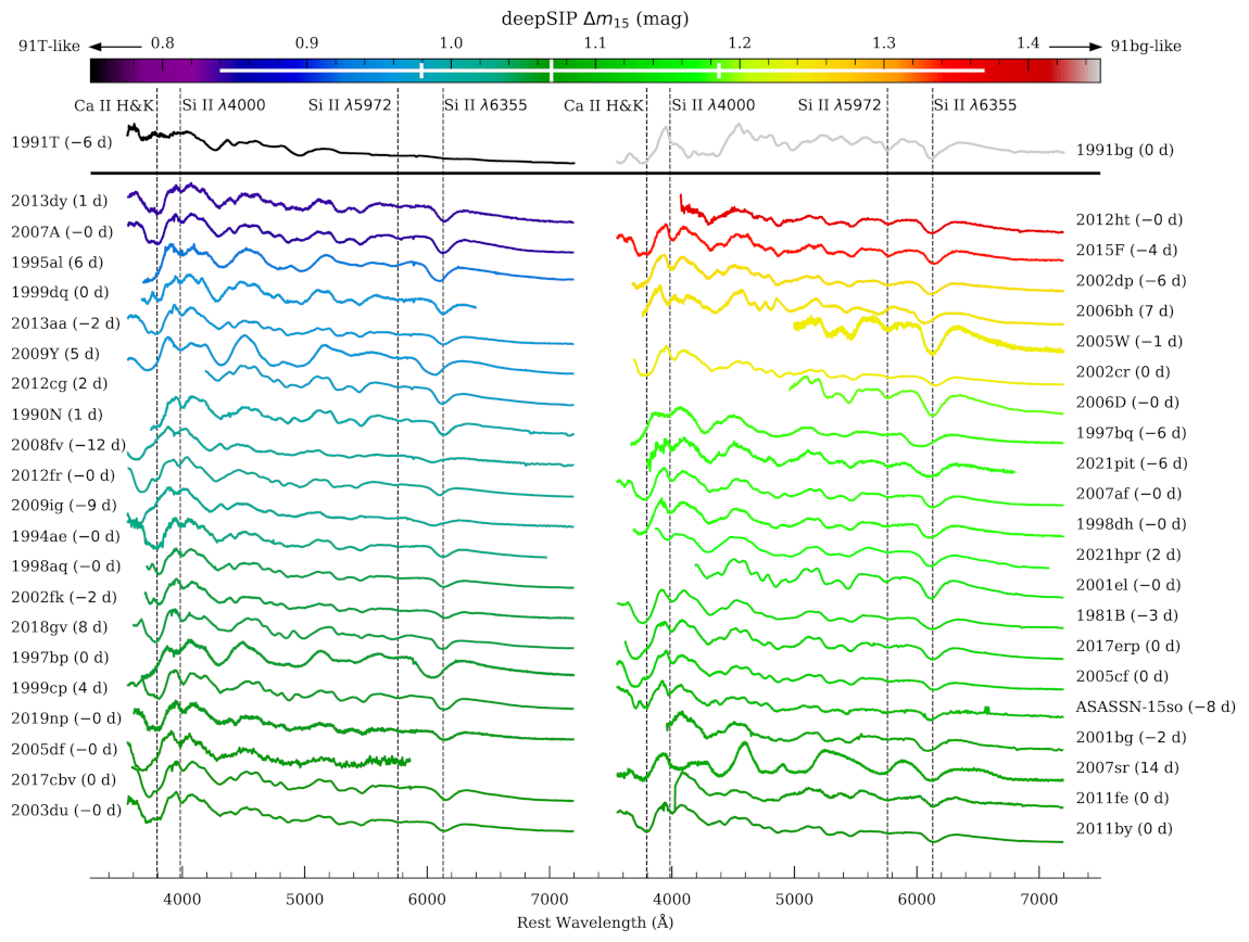
Figure A1: Spectra(scaledfλ)ofall42SNeIainthecalibratorsample,colorcodedbytheirdeepSIPscorecalibratedtothephotometricparameter,Δm15.Asdiscussedinthetext,wefindallcalibratorSNetobeinthenormalrange.PeculiarobjectsSN1991TandSN1991bgbrackettheextremesandareshownforcomparison.

AkeyconcerninstudiesthatutilizeSNIadistances(suchasthisone)isensuringthattheobjectsusedareindeed``normal′′SNeIainthesensethattheycanbestandardizedusingwidth-luminosityrelations

(Phillips:1993).HerewetaketheconservativeapproachofexcludingsubluminousSN1991bg-like(91bg-Filippenko; 91bg-Leibundgut)andoverluminousSN1991T-likeobjects(91T-Filippenko; 91T-Phillips),therebydefining``normal′′SNeIaasthosethatfallwithinthecentral,mostwell-studiedandpreciseregionofthePhillipsrelation.Moreover,weconfirmthenormalcyofourselectedobjectsspectroscopicallybyemployingthedeepSIPpackage(deepSIP),whichprovideshighlyeffective,trainedconvolutionneuralnetworksthat,amongstotherthings,can(i)classifyifaspectrumbelongstoanSNIawitharest-framephasebetween-10dand18dandlight-curveshape(parameterized by SNooPy’s $\Delta m_{15}$ parameter; see SNooPy, for more details)between0.85and1.55mag,aconservativelynarrowwindowcorrespondingto``normal′′objects,and(ii)predict(withuncertainties)quantitativeΔm15values.Becauseweknowtherest-framephaseofeachspectruminoursamplefromthelight-curve-derivedtimesofmaximumbrightness,distinctionsmadebytheaforementionedclassifierprovideadirectprobeiftheSNeIainoursamplearespectroscopicallynormal.ThecalibratorSNeIahaveDeepSIPΔm15valuesbetween0.84and1.37mag.

Wefindthatonlytwospectradonotsatisfythistest,oneofwhich(SN2008fv)isexpectedowingtoitbeingthesolecaseinoursamplewherethespectrumisataphaseearlierthan-10d.Theothercase(SN1997bq)ismostcertainlyspectroscopicallynormal

(see Blondin2012).ThefactthatthissinglefalsenegativeisobtainedisnotunexpectedbecauseindevelopingdeepSIP,deepSIPtunedthedecisionthresholdofthemodelwithaneyetotheirsubsequentscientificusecaseinwhichfalsepositives(i.e.,classifyinganSNIaasnormalwhenitactuallyisnot)representafarworseerrorthanfalsenegatives(i.e.,failingtoclassifyanSNIaasnormalwhenitactuallyis).Wevisualizetheentirespectralsamplealongwithrepresentativenear-maximum-lightspectraofSN1991bgandSN1991Tforreference,colorcodedbydeepSIP-predictedΔm15value,inFig.A1.

A.2 PhotometricProperties

InFig.

A2weshowthedistributionsoftheSALTIIcolor(c)andshape(x1)parameters,aswellasthehostmasses,forthecalibratorsampleandforthreeHubble-flowsamples:(1)thebaseline0.0233<z<0.15spiralsampleandthetighterqualitycuts​|c|<0.15,​|x1|<2;(2)thesameredshiftrangeforallhosttypesandthePantheon+standardqualitycuts​|c|<0.3,​|x1|<3;and(3)asampleofalltypestoz<0.8andstandardqualitycuts.Itcanbeseenthatthesamplesarewellmatchedinthemean,withthebaselinesamplebettermatchedinbreadthtothecalibratorsampleowingtothetighterqualitycuts.Asaresultofthisinvestigation,weconcludethateachSNinthecalibratorsampleisunambiguouslynormalandthuscanbereliablystandardizedtowellmatchthebaselineHubble-flowsample.

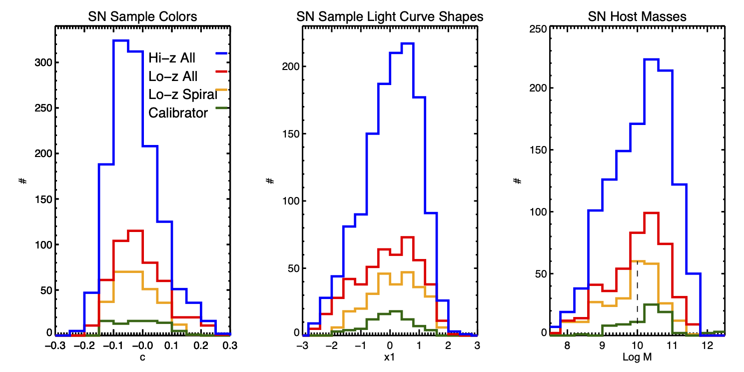
Figure A2: SNIaandhostpropertiesforthecalibratorsample(green)andthreeHubble-flowsamples.Thecolor(leftpanel)andlight-curveshape(middle)distributionsareingoodagreementasdiscussedinthetext,particularlyforthebaselinesample(Lo-zSpiral,orange)whosequalitycutslimitsare​|c|<0.15and​|x1|<2.TherightpanelshowsthehostmassincludingatruncationoftheLo-zsample(dashedline)withvaluesforthisandotherhostpropertiesinTable9.

Appendix B IndependentTestsofCepheidPhotometry

B.1 AperturePhotometry

ThephotometryofCepheidspresentedhereisderivedfromasetofstandardproceduresreferredtointheastronomicalliteratureas``scenemodeling′′or``crowded-fieldphotometry.′′ThesemethodsuseanempiricaldescriptionofthePSFtomodelunresolvedsources(i.e.,stellarprofiles)bycomparingimagepixelstoamodelconstructedfromthesuperpositionofPSFs,eachwithitsownXandYcoordinateandamplitudeaswellastheconstantlevelofthebackground.Theinitialsetofsourcesandtheirpositionsmaybederivedfromtheimageoracatalog.Thisapproachoffersgreaterprecisionthanfixed-aperturephotometry(i.e.,summingfluxinanaperture),asitcanseparatetheblendedfluxofdistinctsourcesandadditionallyimprovestheSNRbytheoptimalweightingofsourcepixels.Biasresultingfromtheinabilitytoresolvenearly-coincidentbackgroundsourcesfromtheCepheidcanbedeterminedstatisticallybyaddingartificialstarsofknownfluxtothescene.Thisbiasisreallyjustthemeanlevelofthefluctuatingbackground.Uncertaintiesaremeasuredfromthedistributionsofrecoveredartificialstars.FrequentlyusedsoftwarepackagesthatenablethisapproachincludeDAOphot,DoPHOT,DolPhot,HSTphot,andRomaphot.Ingeneral,theuseofthesedifferentpackageshasbeenshowntoyieldsimilarresultssubjecttothesettingsforwhichthesepackagesareemployed.However,itisvaluabletohavearobustcross-checkoftheaccuracyofphotometrymeasuredwiththesetechniquesusingasimplerapproachthatiseasilyreplicatedbyotherswithoutreferencetoanyspecificpieceofsoftware.Suchamethodisaperturephotometrywhich,thoughlessprecise,providesastrongtestoftheaccuracytheCepheidphotometryreportedabove.Sinceaperturephotometrycannotreadilyseparatesuperimposedsourcesindenseregions,afewconsiderationsdescribedherearenecessarytoproduceaccurateaperturephotometry.(1)Smallaperturesarerequired,heresetto1.4drizzledpixels(0.′′11)inradius,alongwithanaperturecorrectionderivedfromourPSFmodeltoestimatethefluxoutsidetheaperture.(2)Welimitthecomparisonto1/3oftheCepheidsamplewiththelowestsurfacebrightness,asamplelargeenoughtomeasureH0butwhichstillhaslessbackgroundandthusgreaterprecision.(3)WeuseameanofthepixelsinanannulusaroundeachCepheidtodeterminethesky,ratherthanthemodeormedianwhicharemorecommonlyusedinsparseregions.Thislaststepisveryimportantforderivingaccurateaperturephotometryinthepresenceofafluctuatingbackground.Indenseregions,themeanoftheskyisanunbiasedestimatorofthelevelbeneathasource,asitincludesboththespatiallyconstantbackgroundaswellasthemeanlevelofsuperimposedsources.Incontrast,themodeormedianofthecrowdedskyoranystatisticcalculatedafterfittingandsubtractingvisiblestarsnecessarilyunderestimatestheskyunderthetargetsourcewherewecannotresolveorsubtractblendedsources.WeassumethepositionoftheCepheidwaspreviouslyidentifiedfromsparse,high-contrastopticalimages,asisthecasefortheSH0ESprogram.WemeasuredaperturephotometryoftheCepheidsusingthesameimages(beforeremovinganybackgroundlevel)usedforthePSF-basedphotometryandthesame,fixedCepheidpositions.Theskyvaluewassettothesimplemeanoftheskypixelsinanannulusbetweenradiiof15and25pixelsfromeachCepheid.Fig.

B1displaysacomparisonoftheapertureandPSFphotometryfortheCepheidsasafunctionofPSFmagnitude,showingagreementwithinthesamplemeanerrors.

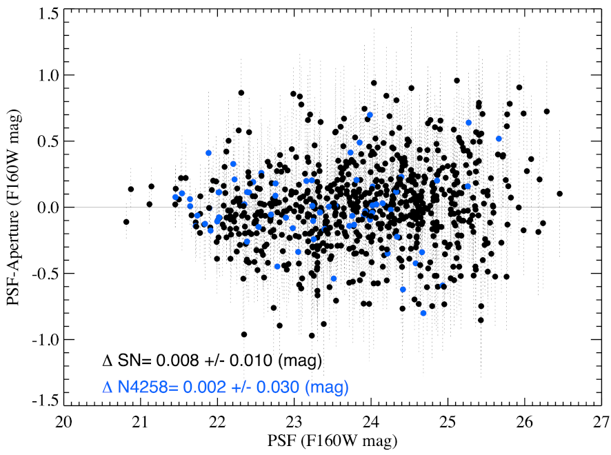
Figure B1: ComparisonofPSFphotometry(withbackgroundsfromartificialstars)forCepheidsinSNhosts(black)andNGC 4258(blue)usedhereandbasicsmall-aperturephotometrywithbackgroundsfromthemeanpixelinalocalannulusasdiscussedinthetext.

WecanmakeafewadditionalobservationsaboutthecomparisonthatclarifiestherelationshipbetweenthestatisticsusedtomeasuretheskyinaperturephotometryandthecrowdedbackgroundcorrectionsusedtoaccountforbiasinPSFphotometry.SincePSFphotometrysetstheskyasa``floor′′leveladdedtomodeledsources,thePSFskylevelwillbesimilartothemode(i.e.,themostcommonvalueorpeakofthedistributionofskyannuluspixels)oftheskypixelsusedin(uncrowded)aperturephotometry,theuniformlevelofpixelswithoutapparentsources.Therefore,thedifferenceinaperturephotometrycalculatedfromaskylevelusingthemodeormeanoftheskypixelswillbesimilartothecrowdedbackgroundcorrectioninPSFphotometry.Insparsefields,themodeandmeanareequivalentandthecrowdedbackgroundbiasisnegligible.Theasymmetricdistributionofpixellevelsintheskyannulusalsoexplainstheusefulfeaturethatinlog-normalormagnitudestheCepheiduncertaintieswhicharedominatedbytheasymmetricdistributionofskypixelsarerelativelyGaussiantoafewstandarddeviations,asshownin§

3.3.

B.2 ImpactsofImprovementsinPhotometry

Asdiscussedin§3.4,weitemizehalfadozenimprovementsinCepheidphotometryfromthelasttimetheseCepheidsweremeasuredbetween∼6and∼16yrago.MatchingCepheidsbyposition,theerror-weightedmeanofthematchedCepheidsarefainterinSNhostsby0.06magandinNGC 4258by0.04mag(anetdifferenceof0.02magwhenNGC 4258calibratestheCepheidsandH0).FortheLMC,Cepheidsbecamefainterby0.03magbetweenthegroundsampleusedbyR16andtheirreplacementbydirectHSTobservationsinR19.ThemeanchangeinF555W--F814Wwasbelow0.01magforCepheidsinSNhostsandintheouterfieldofNGC