SIRfyN: Single Image Relighting from your Neighbors

Abstract

We show how to relight a scene, depicted in a single image, such that (a) the overall shading has changed and (b) the resulting image looks like a natural image of that scene. Applications for such a procedure include generating training data and building authoring environments. Naive methods for doing this fail. One reason is that shading and albedo are quite strongly related; for example, sharp boundaries in shading tend to appear at depth discontinuities, which usually apparent in albedo. The same scene can be lit in different ways, and established theory shows the different lightings form a cone (the illumination cone). Novel theory shows that one can use similar scenes to estimate the different lightings that apply to a given scene, with bounded expected error. Our method exploits this theory to estimate a representation of the available lighting fields in the form of imputed generators of the illumination cone. Our procedure does not require expensive “inverse graphics” datasets, and sees no ground truth data of any kind.

Qualitative evaluation suggests the method can erase and restore soft indoor shadows, and can “steer” light around a scene. We offer a summary quantitative evaluation of the method with a novel application of the FID. An extension of the FID allows per-generated-image evaluation. Furthermore, we offer qualitative evaluation with a user study, and show that our method produces images that can successfully be used for data augmentation.

1 Introduction

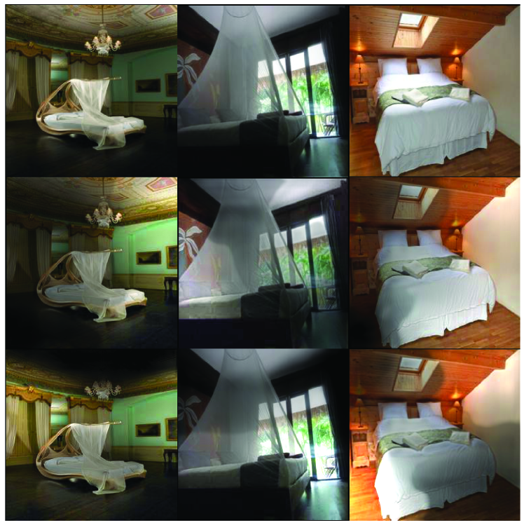
Figure 1: Our method learns to relight images of scenes without any CGI data, paired data or labelled data, using two novel theorems about lighting in scenes. Top: original images. Center and bottom rows show curated relit images of these scenes; each has the same mean intensity as the original image to avoid confusing effects of overall brightness.

When someone switches on a light, the image at the back of your eye changes even when there is no other change. The new shading of the scene in front of you is determined by the shape and material composition of the scene, and by the light source. This paper shows how to relight a scene – we demonstrate a model that can generate images of the scene with random (but plausible) changes in light source. One might expect scene relighting to be easy – decompose the scene into albedo and shading, and replace the shading with another shading field. This approach doesn’t work because shading fields are very strongly related to albedo fields and to shape. For example, sharp boundaries in shading tend to appear at depth discontinuities, which are usually apparent in albedo. This means that it is hard to produce shading fields that apply to a particular scene with elementary methods.

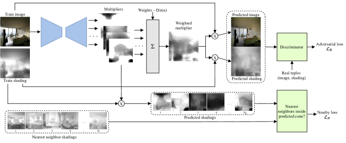
Figure 2: Our network accepts an image and produces a set of multipliers; a relighted image is produced by obtaining a random non-negative set of weights, then forming a weighted sum of these multipliers. There are two main losses: the multipliers should result in a realistic pair of (image, shading) , imposed by an adversary; and the multipliers applied to the original image’s shading field should encode the shading fields of nearest neighbors, a loss justified by two novel theorems Section 4;

An alternative strategy is to use “inverse graphics” – learn to regress geometry, material, etc. against an image using training set that consists of ground truth geometry, material etc. together with computer generated images (CGI). While this strategy may offer an approach to building some kinds of vision system, it is laborious (one must produce the training data) and is not yet reliable. Furthermore, the inverse graphics strategy is intellectually unsatisfying, because it doesn’t explain how a visual agent learns to interpret the rich visual world they see if the agent doesn’t have a CGI training set conveniently to hand.

Instead, we see scene relighting as an unsupervised problem. We train a neural network to produce a set of per-pixel scalings for an image. Each scaling produces a new image under some, likely extreme, illuminant (and, implicitly, a new shading field). A non-negative linear combination of the scalings produces other relighting. Two novel theorems establish that it is possible to estimate these likely relightings from observations of other, similar, scenes. These theorems motivate using a loss that measures how well the predicted shading fields represent shading fields from other, similar scenes. Extensive evaluation shows that (a) our relighted images are diverse and realistic; (b) rejection sampling methods are available that can produce sharp improvements in quality; (c) our predicted shading fields are consistent with observed shading fields; and (d) our strongest method can be used successfully as a data augmentation.

Contributions: We offer the first scene relighting method that requires no data marked up in any form. We offer a novel body of theory showing how perturbations of geometry, albedo and luminaire (a luminaire is an object that emits, rather than simply reflects, light) affect scene radiosity, and that lightings of similar scenes can be used to infer lighting of a given scene. We show how to evaluate our models quantitatively as well as qualitatively. We introduce a variant of the FID that applies to image transformations and gives a per-image estimate of quality.

2 Related Work

Intrinsic image decomposition Decomposition into albedo and shading is well established; evaluation is by comparing predicted lightness differences to human labelled versions, the WHDR score. We use the method of [1] (see that paper for a detailed review of an area whose history dates to the mid 19’th century), which requires no labelled training data or CGI and produces a WHDR of 16.9%, current SOTA for such a method.

Inverse rendering seeks to recover all required data for rendering from an image. Reconstruction methods applied to multiple images are one approach (eg [2]); another is to impose strong parametric models [3]. Alternatively, one could train a regressor using a fixed object class (faces [4]; furniture [5]; birds [6]), CGI of general shapes [7, 8], or multiple images [9]. Very strong reconstructions can be obtained from rendered images [10]; isolated object reconstructions can be relit [11]. Inverse rendering recovers strong scene models for indoor scenes from CGI [12], but we are aware of no successful attempt to change luminaires in images of scenes by relighting an inverse rendering result. In contrast to inverse rendering methods, we use no CGI and no marked up data.

Precomputed radiance transfer (PRT) is a method from computer graphics that builds a relightable representation of a scene by rendering versions with multiple distinct illuminants, producing an estimate of the light transport matrix mapping illuminant representation to relit scene (originally [13]; review in [14]; compare a PRT operator with our EGM, below). The operator can be estimated for real scenes with a projector and a large number of images (a generalization of [15]) or from a collection of outdoor images [16]. There are strong regularizers which can massively reduce the amount of scene data needed (eg [17, 18]). Given relatively few lightings of a scene, a neural network can produce a very good light transport matrix estimate [19, 20]; this is consistent with theorems 1 and 2. In contrast to PRT methods, our estimate requires only one image of a given scene, but must be a great deal less accurate.

Image relighting is now an established task. For scenes, there are workshop tracks (eg [21, 22]), challenges [23, 24] and datasets  [25, 26]. Existing work learns image mappings (pure image mappings as in [27]; depth guided, as in [28]; using wavelets, as in [29]; shadow priors, as in [30]). In all cases, methods are learned with paired data (ie images of the same scene under different illuminations), available in the VIDIT dataset [25] and the MIE dataset [26]. VIDIT data is CGI, and emphasizes point light sources with strong shadows, which are uncommon in indoor scenes. Pairing is necessary to ensure that their method preserves scene characteristics [31, 32]. Chogovadze et al use a multi image dataset and lightprobes to learn a scene relighter, and show the resulting augmentations improve two patch matching tasks [33]. Philip et al. learn geometry aware models to relight outdoor video from renderings under multiple light conditions [34]. Similarly, face image relighting requires multi-illumination data (from real light stages [35]; made using deformable models [36]). In contrast to these methods, we do not use paired data.

Shadow synthesis is now an established task. People in video can be used as scene probes to learn to create shadows for objects inserted in outdoor scenes [37]; methods with sufficient training data can learn to create soft attached shadows for objects that have been inserted into indoor scenes [38, 39]. In contrast to these methods, we use no paired or synthesized data, and we create entire lighting fields.

Global illumination bounds: Section 4 establishes that scenes with similar albedo, luminaire and geometry have similar radiosity. Bounds on the effect of luminaire difference are well known (eg [40], sec 5.3; [41]). Previous results on the effects of albedo changes are rare ( [42] sketch the case for an integrating sphere; [43], p175, has a bound). There are few results on the effect of perturbing geometry; [44] estimate the effect of flat ports on an integrating sphere; [42] argue that sufficiently small deformations of an integrating sphere do not affect its function; and [43], p176, says such results are hard to get.

The illumination cone and its generators (ICGs): The family of images created by lighting a single convex diffuse object, viewed in a fixed camera, with a point source is naturally a convex cone (reflection is linear; irradiance is non-negative). As Kriegman and Belhumeur [15] point out, this fact extends to any diffuse scene. If the observed scene has only a discrete set of normals – for example, a polyhedral object – then the cone is polyhedral and has a finite set of generators (i.e. any element of the cone is a non-negative sum of a finite set of generators). In simple cases, one can recover generators by illuminating the object with different sources. Interreflection and shadowing may mean that the cone is not polyhedral, but experiments suggest that (a) relatively few generators provide a good representation of the cone anyhow ([15], p.8; [45], p.644) (b) the cone is relatively “flat” ([15], conjecture 1; p.12; for convex objects [46]) and (c) illumination cone methods offer strong models of extreme relighting for face images [45].

3 SIRfyN: Methods and Network

At run time, we want to be able to produce multiple realistic relightings from a single image of a scene, without requiring intrinsic image decomposition etc. We will build a network that maps a 256x256x3 color image $I_{V}$ of a scene $V$ to a set of $N_{g}$ multipliers $M_{i}(I_{V})$ (256x256x1 scalar fields). For non-negative $\theta_{i}$ and $\cdot$ broadcast element-wise multiplication, these multipliers will have the property that $M(\theta)\cdot I_{V}=\left[\sum_{i}M_{i}(I_{V})\theta_{i}\right]\cdot I_{V}$ is a relighted version of $I_{V}$. One can think of these multipliers in terms of shading fields, by modelling the image as a product of albedo and shading $I_{V}=A_{V}\cdot S_{V}$; then relighting $I_{V}$ by $M(\theta)$ implies a new shading field $S_{V}\left[\sum_{i}M_{i,V}\theta_{i}\right]$. So predicting $M_{i}(I_{V})$ from $I_{V}$ yields an encoding of the shading fields we expect for that scene – equivalently, estimates of generators for the scene’s illumination cone.

Network: We predict multipliers using a network to obtain $\left[M_{1}(I),\ldots,M_{N_{g}}(I)\right]=N(I;\phi)$. We implement $N(I;\phi)$ using a u-net, with skip connections (details in supplementary; $\phi$ parameters). The output layer forms a multiplier directly from activations, with housekeeping losses to ensure that multipliers are non-negative.

The key trick is obtaining losses to train such a network. Section 4 sketches two novel theorems we rely on (proved in detail in supplementary). Theorem 1 states that, for two scenes $V$ and $V^{\prime}$ with similar geometry, illumination and albedo, the difference between radiosity $B_{V}$ and $B_{V}^{\prime}$ is bounded (despite the effects of interreflections). Now radiosity is linear in illumination and images are linear in radiosity, so we can model different relighted images of the same scene with some linear operator, which is easily estimated if we have multiple images of the same scene under different lights. We don’t have such images, but Theorem 2 states that the expected future error of using images of similar scenes in place of images of the original scene is bounded.

We can now test whether the network is producing sensible multipliers with theorem 2. Theorem 2 means that, for the shading field $S_{V}^{\prime}$ of each image of a similar scene $I_{V}^{\prime}$, there should be some non-negative $\theta_{V^{\prime}}$ so that $S_{V}^{\prime}\approx S_{V}\left[\sum_{i}M_{i}(I_{V})\theta_{V^{\prime},i}\right]$.

Finding images of similar scenes: It is not practical to enforce the exact constraints of section 4, but the intention of these constraints are that a nearby image should depict a scene of similar shape to the original scene. GIST features were hand-tuned to encode the overall shape of a scene [47], and we use the 20 nearest neighbors in GIST features. We have not attempted to optimize further, but informal experiments with learned embeddings were not successful, and we expect that incorporating an albedo matching term might help.

Exploiting images of similar scenes: Assume we have $k$ images which can be used to estimate generators for an image $I_{V}$. There should be some non-negative ${{\bf w}}$ such that the shading field $S_{i}$ of the $i$’th such image is encoded by the multipliers, so $S_{i}\approx S_{V}\left[\sum_{i}M_{j}w_{j}\right]$. Geometrically, we require that each $S_{i}$ lie inside the cone generated by $\left[S_{V}M_{1},\ldots,S_{V}M_{N_{g}}\right]$. There are some subtleties involved in deriving a loss from this constraint. We do not want $2S_{i}$ to be “further outside” the cone than $S_{i}$ is, so the loss needs to be independent of the scale of the shading field. We achieve this by rescaling all shading fields to have mean 0.7 (the value is arbitrary, and affects only the scale of the loss). The nearby loss on multipliers can be written as

$${\cal L}_{N}(I_{V},\phi)=\sum_{i\in{\cal N}}C(S_{i},M(I_{v}))$$

for ${\cal N}$ the neighbors of $I_{V}$ and

$$C(S_{i},M(I_{V}))=\begin{array}[]{c}\mbox{min}\\ {{\bf w}}|{{\bf w}}>0\end{array}{\mid\!\mid\!{S_{i}-\sum_{j}S_{V}M_{j}(I_{v};\phi)w_{j}}\!\mid\!\mid_{2}}^{2}$$

but this is difficult to evaluate (the non-negativity constraint means the value is a solution to a quadratic program). We estimate $C(S_{i},M(I_{V}))$ by solving for ${{\bf w}}$ using least squares; clipping to ensure ${{\bf w}}\geq 0$; then taking a $N_{gd}$ steps of projected gradient descent in $\theta$. This yields a usable approximate loss.

Realistic scene preserving shading: It is important that, for predicted multiplier $M(\theta)$, the image $M(\theta)I_{V}$ should look like a relit version of $I_{v}$. We impose this constraint using an adversarial loss to adjust the joint distribution of (predicted shading, predicted image) to match the best estimate of the true distribution. Here ${\cal L}_{R}(I_{V};\phi)$ is the value of an adversary that compares generated tuples $(M(\theta)S_{V},M(\theta)I_{V})$ to real tuples $(S_{I},I)$ and $S_{I}$ is the shading field of image $I$, estimated using the method of [1]. The discriminator score (we use a hinge loss, as in [48]; details in supplementary) depends only on local neighborhoods, as in PatchGAN [49], and the size of the neighborhood has important effects on results.

Extrapolation with a barrier: If nearby images for a given image have relatively similar shading fields, the nearby loss will not encourage diversity because it does not force the $M_{V,j}$ to be different. But we want to extrapolate and force the new shadings to be as extreme as possible. Write int for the operator that computes the intensity of an image, $\overline{I}$ for the pixelwise mean of an image, $P_{V}=\mbox{int}(M_{V}I_{V})$ and $Q_{V}=\mbox{int}(I_{V})$. We use

$${\cal L}_{B}(I_{V};\phi)=\overline{L}\mbox{ where }L=-\log\mid\!\frac{P_{V}}{\overline{P_{V}}}-\frac{Q_{V}}{\overline{Q_{V}}}\!\mid$$

as a diversity loss; this forces multipliers to be different from 1, but may result in unrealistic relightings if overweighted.

Realism housekeeping: we require that any pixel in $R$ should be non-negative (${\cal L}_{U}(R)$), and less than one (${\cal L}_{O}(R)$), and achieve this with simple one-sided quadratic losses. Note that this constraint applies to relighted images, rather than shading fields – applying the constraint to shading fields will lead to regions with dark albedo being consistently dark. We show the network $A$ as well as $I$ so that it can anticipate this loss and produce very bright shading at locations where the albedo is dark.

Overall loss: the loss is then:

$${\cal L}={\cal L}_{N}+\lambda_{B}{\cal L}_{B}+\lambda_{O}{\cal L}_{O}+\lambda_{R}{\cal L}_{R}+\lambda_{U}{\cal L}_{U}$$

4 Theory: ICGs and EGMs

Light in diffuse scenes: The brightness of each pixel in the camera is determined by the radiosity at the corresponding scene point. Write $\rho({{\bf u}})$ for albedo at the point on the geometry parametrized by ${{\bf u}}$, $E({{\bf u}})$ for the diffuse emittance of that point (only non-zero when the point is actively emitting light, so a point on a luminaire with non-zero weight), and $B({{\bf u}})$ for the radiosity at ${{\bf u}}$. Write ${\bf D}_{\rho}$ for the linear operator that maps $f({{\bf x}})$ to $(\rho f)({{\bf x}})$. Then standard diffuse interreflection theory (see, eg [50, 51, 52, 53]) gives $B=E+{\bf D}_{\rho}{\bf K}B$, equivalently $(I-{\bf D}_{\rho}{\bf K})B={\bf R}B=E$ where ${\bf K}$ is a bounded linear integral operator. This yields a Neumann series solution $B={\bf R}^{-1}E=E+{\bf D}_{\rho}{\bf K}E+({\bf D}_{\rho}{\bf K})^{2}E+\ldots$ which should be interpreted as “emittance+direct term+one bounce+…”; for most practical geometries and albedos, relatively few terms at relatively poor spatial resolution yield an acceptable solution (eg [54], reviews in [41, 55]).

ICGs from diffuse interreflection theory: Assume that a scene has $N_{e}$ luminaires, so that $E=\sum_{i}\theta_{i}E_{i}$ with $\theta_{i}\geq 0$ the intensity of the luminaires. We choose ${\mid\!\mid\!{E_{i}}\!\mid\!\mid_{2}}=1$. Because the solution is linear in the emittance, we can write $B({{\bf u}};\theta)={\bf R}^{-1}\sum_{i}\theta_{i}E_{i}=\sum_{i}\theta_{i}{\bf R}^{-1}E_{i}=\sum_{i}\theta_{i}B_{i}({{\bf u}})$ – if we know the solution for each luminaire separately, we can construct a solution for any linear combination of luminaires. If we have one image of the scene for each luminaire, where the image is illuminated by that luminaire alone, we can generate an image from this viewpoint for any combination of the luminaires. But we do not have these images.

Similar scenes with similar luminaires have similar radiosity: We assume that all relevant reflection is diffuse; it is likely that this can be generalized (discussion). A scene $V$ is a tuple of geometry, albedo and luminaire model; write $V=\left({\cal G},\rho,{\cal E}\right)$, where ${\cal E}$ is the luminaire model. The geometry ${\cal G}$ consists of a set of surfaces parametrized in some way and a 2D domain for that parametrization; write ${\cal G}=({{\bf s}}({{\bf x}}),{\cal D})$. The luminaire model captures the idea that lighting in a particular scene may change. We have ${\cal E}=\left(E_{1},\ldots E_{N_{e}},P(\theta)\right)$ for a set of potentially many basis luminaires and a probability distribution over the coefficients. This information implies a probability distribution over luminaires for the scene $P(E)$. Similarity: Two scenes $V$ and $V^{\prime}$ are similar if: there is some affine transformation so that ${\cal G}^{\prime}({\cal G},{{\cal A}},{{\bf b}})=({{\cal A}}{{\bf s}}({{\bf x}})+{{\bf b}},{\cal D})$. $E^{\prime}_{i}({{\bf x}})=E_{i}({{\bf x}})$ ; and $P_{V}(E)$ and $P_{V^{\prime}}(E)$ the same. Consider some lighting $E_{V}$ of $V$ and a different lighting $E_{V}^{\prime}$ of $V^{\prime}$: Theorem 1 (below) establishes that if $V$ and $V^{\prime}$ are similar, and $E_{V}$ and $E_{V}^{\prime}$ are similar, then $B_{V}$ will be close to $B_{V^{\prime}}$.

Theorem 1: For $V=({\cal G},\rho,E)$ and $V^{\prime}=({\cal G}^{\prime}({\cal G},{{\cal A}},{{\bf b}}),\rho^{\prime},E^{\prime})$, where $\epsilon_{E}{\mid\!\mid\!{E}\!\mid\!\mid}={\mid\!\mid\!{E-E^{\prime}}\!\mid\!\mid}$, $\epsilon_{\rho}=\mbox{sup}_{\cal D}{\mbox{abs}{{\left[\rho-\rho^{\prime}\right]}}}$, $p=\mbox{sup}_{\cal D}\rho$, $p^{\prime}=\mbox{sup}_{\cal D}\rho^{\prime}$, $c$ is the condition number of ${{\cal A}}$ (ratio of largest to smallest eigenvalues), we have:

$${\mid\!\mid\!{B_{V}-B_{V^{\prime}}}\!\mid\!\mid}\leq c_{1}(\epsilon_{E},\epsilon_{\rho},p,p^{\prime},c)$$

Proof: Elaborate, relegated to supplementary, which gives the form of $c_{1}$

The effective generator matrix (EGM) of a scene: Choose some $N_{o}$ element orthonormal basis to represent the possible radiosity functions for the scene (if $N_{o}=N_{e}$, the representation is exact, because there is a finite dimensional space of luminaires). In this basis, any particular radiosity $B({{\bf x}})$ has coefficient vector ${{\bf b}}$. Write ${{\bf b}}_{i}$ for the coefficient vector representing $B_{i}({{\bf x}})$; and ${{\cal B}}=\left[{{\bf b}}_{1},\ldots,{{\bf b}}_{N_{e}}\right]$. For any $r\leq N_{e}$, an effective generator matrix for scene $V$ is an $N_{o}\times r$ orthonormal matrix ${{\cal M}}_{V}$ such that for any illumination condition producing radiosity represented by ${{\bf b}}$ , there is some ${{\bf w}}$ such that the radiosity represented by ${{\cal M}}_{V,r}{{\bf w}}$ is similar to the actual radiosity field. In particular, we want

$${\cal L}({{\cal M}}_{V})={{{{\mathbb{E}}}}_{{\theta\sim P(\theta)}}{{\left[{{\mbox{inf}_{{{\bf w}}}{\mid\!\mid\!{{{\cal M}}_{V}{{\bf w}}-{{\cal B}}\theta}\!\mid\!\mid_{2}}^{2}}}\right]}}}$$

to be small; ${{\cal M}}_{V}$ is clearly not unique. Now if we have $k$ radiosity fields for a scene under different, unknown, illumination conditions, for $k$ very large, where for each $\theta_{i}\sim P(\theta)$ (which is not known). We could estimate an EGM by replacing the expectation with an average, and minimizing. But we do not have $k$ images of the same scene.

Estimating an EGM: An EGM can be estimated from radiosities obtained from similar scenes. Write ${\cal L}_{T}({{\cal M}})$ for the true expected error of using an EGM ${{\cal M}}$ to represent the radiosity of a scene. Theorem 2 shows that substituting an estimate $\hat{{{\cal M}}}_{O}$ obtained by using $k$ radiosities in total, taken from distinct similar scenes, for the best (but unknown) effective generator matrix ${{\cal M}}_{O}$ incurs bounded error. This means we can use estimates from similar scenes with confidence, if the scenes are similar enough.

Theorem 2:${\cal L}_{T}(\hat{{{\cal M}}}_{O})-{\cal L}_{T}({{\cal M}}_{O})$ is bounded.
Proof: Elaborate; relegated to supplementary, which provides the bound.

Image loss from theory: Note first that theorem 2 applies to images as well as to scenes. If one views a scene through a fixed camera, the camera is a linear mapping (taking scene radiances to pixel values) and it is bounded. The result is very powerful, because it says that an estimate of the generator matrix for a given image can be obtained from enough images of similar scenes — take the shading fields $S_{i}$ of similar scenes and form a ${{\cal M}}$ that minimizes

$$\sum_{i}{\mbox{inf}_{{{\bf w}}}{\mid\!\mid\!{{{\cal M}}{{\bf w}}-S_{i}}\!\mid\!\mid_{2}}}.$$

Using this approach directly is inconvenient because it means we need to find similar images at inference time. Instead, we derive a loss from Theorem 2 and use a network to predict the generator matrix.

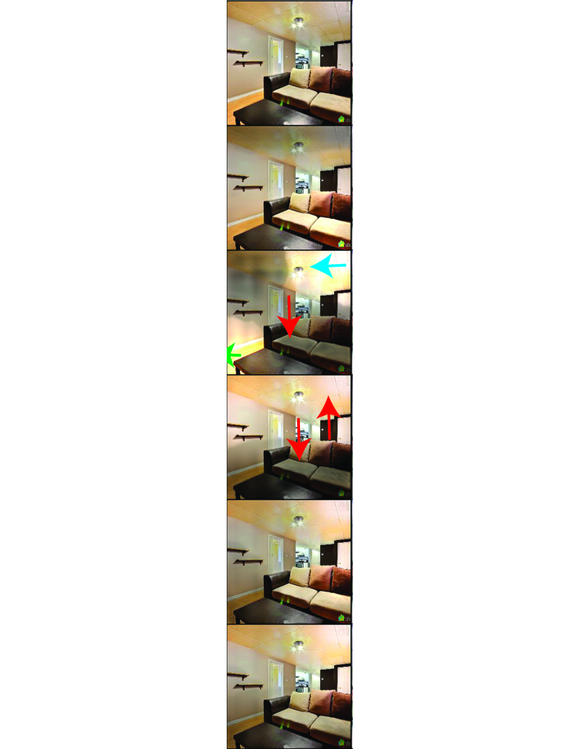
Figure 3: Images relighted at $\alpha=0.1$ (more variable; left; cf $\alpha=0.5$ less variable in supplementary) and the first five multiplier fields for each right. Top row: shows original images; the following five rows are random relights, not curated. A number of important effects are notable: green shadow removed or replaced; red significant brightening or darkening of one surface, registered to geometry. yellow suppression or enhancement of a gloss effect; blue suppression or enhancement of a luminaire. All relights are shown at the same mean intensity as the original image, to ensure that effects are not masked by overall shift in brightness. Multiplier fields are scaled so that one is mid-grey, less than one darker, greater than one brighter. Recall relights are combinations of multipliers, with coefficients drawn as in Section 3

5 Quantitative Evaluation for Relighting

Realism in current image generators is typically measured with the FID [56]. One embeds a set of generated images, then computes the Frechét distance between the resulting points and an embedding of a set of real images. We use the standard VGG embedding of [56], with dimension $d_{f}=2048$. This is an estimate of the difference between the distributions from which the samples were taken; smaller values are better. As [57] show, the FID estimated from a finite set of points is biased by a $1/N$ term that depends on details of the generator, but straightforward extrapolation methods remove this bias successfully to produce ${\mbox{FID}_{\infty}}$. An important difference between image relighting and image generation is that relighting should map the collection of real images to itself, preserving frequencies etc. (loosely, relighting is an isomorphism). In turn, this means that the FID between a set of images ${\cal O}$ and a relighted set ${\cal R}$ of images should be zero, so ${\mbox{FID}_{\infty}}({\cal O},{\cal R})$ should be zero up to sampling error. Note strong realism scores can be obtained by not changing the original image much.

Diversity: We must also evaluate whether relighted versions of an image are actually different from the original image. We measure diversity by comparing relighted images to the original. We rescale the relit image to have the same mean as the original image, so that just scaling images will get zero diversity score. Write $N_{t}$ for the total number of pixels in relighted images; we score diversity with $MSD$, computed as

$$MSD_{\hat{\theta}}=\sqrt{\frac{1}{N_{t}}\sum_{i\in\mbox{images}}\overline{D}^{2}_{i}},$$

where $D_{i}=(I_{i}-R_{i}(\overline{I}_{i}/\overline{R}_{i}))$. Note quite unreasonable shadings may have high diversity scores.

Local FID: Because relighting is an isomorphism, we can recover a per-image measure of quality. Assume we obtain ${\cal R}$ from ${\cal O}$ by relighting a single image $I_{k}$ to obtain $R_{k}$ and compute ${\mbox{FID}}({\cal O},{\cal R})$. This value – which is non-negative, and is ideally zero – measures the extent to which the relighted image is realistic. Furthermore, different relightings of the same image will have different values. This value is the local FID of image $R_{k}$. This local FID strongly reflects human preferences (Figure 4; people reliably prefer images with smaller local FID). Computing the local FID requires care; the supplementary shows how.

Figure 4: Left: Model selection is by inspecting plots of ${\mbox{FID}_{\infty}}$ against MSD for three different values of $\alpha$ (0.01, 0.1, 3.0). Best behavior is down and to the right (low ${\mbox{FID}_{\infty}}$, high MSD). We show some effects here; more in supplementary. Models seem largely to stick fairly close to a Pareto frontier. The pixel uniformity loss is unhelpful (supplementary) and so its weight $\lambda_{P}$ is 0 except where noted. There is a bias variance tradeoff in the number of generators; $N_{g}=15$ gives more diversity for weaker quality, etc.; $N_{g}=10$ is about right, compare  [46]. Training at 256x256 produces notable improvements (compare chosen at 128 with chosen at 256). A pure mapping of pixels (1x1 convolutions, trained with the same losses; 1D control) is a lot weaker than any of our models. Horizontal line shows ${\mbox{FID}_{\infty}}$ of random splits of data (Spl baseline); dashed are 1-sd limits (mean=0.99, sd=0.027). Center left: Difference in LFID is a good predictor of human subject preferences. Points show probability that A is selected against difference value, for each of 500 quantiles of LFID difference and a total of 50000 preference tests. Curve shows a logistic regression predictor; the fit would likely be improved by removing large differences in LFID. Choice of scale has occluded two data points (one at very far right; one at very far left). Center Right: LFID plotted against MSD for 100 randomly relighted samples for 10 test images. Note the wide spread; a rejection sample (which seeks large MSD for low LFID, say), is likely to be successful. Right: Rejection results: RTop: original images; RCenter: relights with highest MSD for $LFID<25000$ (so most different from original at fixed quality); RBottom: relights with lowest LFID for $MSD>0.2$ (so best at fixed difference from original). Best viewed in color at high resolution, compare supplementary material. All relights are shown at the same mean intensity as the original image, to ensure that effects are not masked by overall shift in brightness.

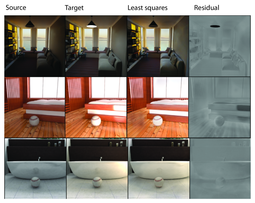
Figure 5: We investigate the plausibility of generators by: rendering CGI scenes under two lights; computing the generators for the source; constructing weighted sum of generators that yields a least squares fit to the target; then comparing target to the least squares. The residual error in intensity is shown on a scale where white is 1; mid grey is 0; and black is -1. Note relatively good fits, suggesting that for the cases we have investigated, generators are a reasonable fit. Quantitative: over a total of 11 pairs (22 tests), for a dataset we will provide, we find average metrics between the least squares prediction and the target of RMSD: 0.0503 PSNR: 26.6 LPIPS: 0.0648, suggesting quite successful prediction of the target by source generators.

6 Experimental Details

Datasets: No markup is required. Training albedos are obtained with the method of [1]. We train with images from the LSUN Bedroom dataset ([58]), resized as described. We use 20,000 images to train the generator (augmented by crop and resize and horizontal flips) and train the discriminator with 20,000 distinct images (to prevent shading “leaking”). Nearest neighbors are drawn from 100,000 LSUN Bedroom images, and are augmented in the same way (so when a training image is cropped, the same crop is applied to each nearest neighbor). We use 20 nearest neighbors for each image to compute ${\cal L}_{N}$.

Relighting weights in training: During training we must ensure that any non-negative combination of multipliers results in a realistic image; we do so by randomly selecting one multiplier per image in a batch, and passing those to the adversary.

Choice of hyperparameters: For model search purposes, we train our network at 128x128. Simple qualitative experiments suggest the model is not particularly sensitive to the choice of $\lambda_{R}$, $\lambda_{U}$ and $\lambda_{O}$,and we have used $1,100,100$. Simple qualitative experiments show that training without projected gradient descent ($N_{gd}=0$) fails reliably; more than one step ($N_{gd}>1$) slows training without offering any obvious benefit. Other hyperparameters that have significant effects are: $N_{g}$, $\lambda_{P}$, $\lambda_{B}$ and the scale of the discriminator. Figure 4 plots ${\mbox{FID}_{\infty}}$ against MSD for a variety of methods at three different values of $\alpha$ (FID vs MSD and detailed comparisons in supplementary). In summary, we have: a small scale discriminator is better; $\lambda_{B}=5$ is about right; there is a bias-variance tradeoff for $N_{g}$, and $N_{g}=10$ is about right (cf [46]).

Inference and equivariance: Our chosen network is trained on 256x256 images. The model should be sensitive to geometry (and is - supplementary), so resizing an image that isn’t square should be dangerous (and is - supplementary), and so we always work with 256x256 images, and crop (rather than resize) as required. We model the weights as distributed according to a symmetric Dirichlet distribution with concentration parameter $\alpha$. Then we generate relighted images by: drawing a sample of weights; computing multipliers; computing a weighted combination of multipliers; and multiplying by the image.

Baselines and Controls: There are no meaningfully comparable methods. However, sampling error, etc., means it is important to have baselines for “low” and “high” values. We use two baselines. Spl: we evaluate sampling variance in ${\mbox{FID}_{\infty}}$ by computing the ${\mbox{FID}_{\infty}}$ between random splits ${\cal O}_{i}$ of the image set, and obtain $F_{\mbox{spl}}={\mbox{FID}_{\infty}}({\cal O}_{i},{\cal O}_{j})$. This yields a “low” FID estimate. 1D: to exclude the possibility that our relighting method simply maps pixel values, we train a relighting method using only 1x1 convolutions.

7 Results

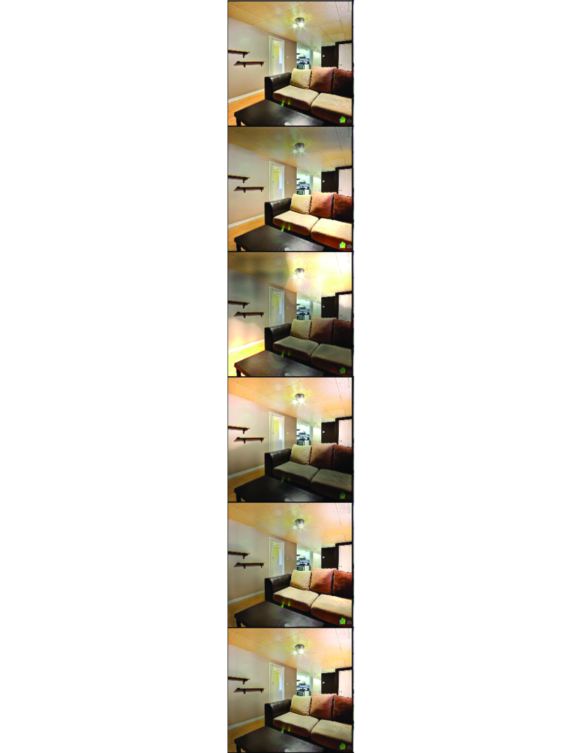
Figure 10: Images relighted at $\alpha=0.1$ (more variable; left; cf $\alpha=0.5$, less variable, $\alpha=0.01$, much more variable, in Fig 11) and the first five multiplier fields for each right. Notice how the multipliers are keyed to structures in the image – the method “knows” some geometry and radiometry. Reproduced from Fig 3 of main paper, without arrows, for reference.

Qualitative analysis: Figure 10 shows five random relightings of five scenes, together with the relevant multipliers. These random relights, not curated, show: shadows removed or replaced; significant brightening or darkening of surfaces, registered to geometry; suppression or enhancement of gloss effects; and suppression or enhancement of luminaires. The model is clearly capable of substantial, non-obvious relightings that look realistic, and can clearly cope with a very diverse range of surfaces. Relightings include overall changes of brightness, but are not confined to them. The model appears to have some form of geometric knowledge (it often changes the lighting of horizontal and vertical surfaces differently).

The uses of LFID: If relighting is to be used for data augmentation, one seeks relightings that make large changes to a scene. Figure 4 shows the results of a rejection sampling method that seeks the best LFID for MSD over a threshold; and the largest MSD for LFID below a threshold.

Relighting is a successful data augmentation: Chogovadze et al show relighting augmentations improve two patch matching tasks [33]. Table I shows that our relighting augmentations improve performance on a classification task, with greater impact when the dataset is small (to be expected – relighted images contain information from nearest neighbors, redundant when there are enough images). Improvements for the “*-room” categories exceed those for others, suggesting the augmentation – which is learned on bedrooms – generalizes, but not to arbitrary scenes. Table II shows that our relighting augmentations improve performance on a self-supervised learning task. Note that, while our relighter sees only bedroom images, table I suggests strongly that it produces acceptable relightings for other scenes, likely a consequence of the common geometry of rooms (see also supplementary).

Egs Relight Top-1 acc TP “*room” TP not “*room” 1000 No 51.3 51.2 51.3 1000 Yes 51.5(+0.2) 53.9 (+2.7) 51.4(+0.1) 100 No 35.7 37.2 35.6 100 Yes 36.2(+0.5) 38.9 (+1.7) 36.0 (+0.4) 10 No 24.9 25.8 24.8 10 Yes 25.5(+0.6) 27.1(+1.3) 25.4 (+0.6)

TABLE I: Relighting augmentations are helpful in a classification task. We use an imagenet pretrained resnet 50 feature stack (cf [59]) to classify images from places365 ([60]; 365 classes). For each case, we use the given number of randomly selected examples per class (at 10 per class, overfitting is pronounced; we average over multiple training runs to suppress variance); augment with crop, flip, color jitter and, if using relighting, relight[alpha=0.1]. Note the effect of relighting is more pronounced with few examples. There are 28 classes named “*room”; notably, the test precision (TP) for these classes improves more than for others.

Augs Top-1 acc Top-1 acc relight A 16.1 16.3 B 16.1 16.5 C 14.2 15.2

TABLE II: Relighting augmentations are helpful in a self-supervised learning task. We train a feature stack using SIMCLR [61] with three different augmentation conditions: A - original from the paper; B - without left/right flip; C crop with scale in [0.36, 1]. For relight, we use pairs of images with distinct relights. We train on 10K LSUN bedroom images, freeze, then train a linear readout on places365 36K; then evaluate. Note that using relighted images reliably offers a small gain.

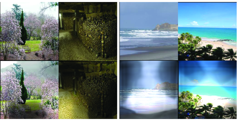
Figure 6: Rough shape – rather than scene label – seems to be key to this method’s success. Left: images (top) from Places365 categories botanical_garden and catacomb and relightings (bottom); because the rough shape is like that of a bedroom, the relightings are quite good. Right: images from ocean; relightings are inaccurate, likely because the model cannot deal with this class of spatial layout; note how the relightings echo the geometry of a room.

8 Discussion

Further work will likely include: using these results to regularize PRT estimation; investigating the effects of architectural choice on the network; and reestimating nearest neighbors with generator estimates. Limitations: Some relightings are clearly not present, and generalization to other scenes is variable (Figure 6). We have no procedure for improving the model, save collecting more (unlabelled) data.

Negative social implications: Convincing fake images can pollute (say) the news media; but our method offers only relighting, rather than the much more dangerous insertion or deletion editing. Experiments required approx 250 hours of time on a single GTX3090 from method inception to submission. The datasets used either do not contain, or are not known to contain, personally identifiable or offensive material. A total of $150 was paid to Amazon mechanical Turk workers for image labelling; no personally identifiable information was collected.

Appendix I: Further variants and fuller comparisons

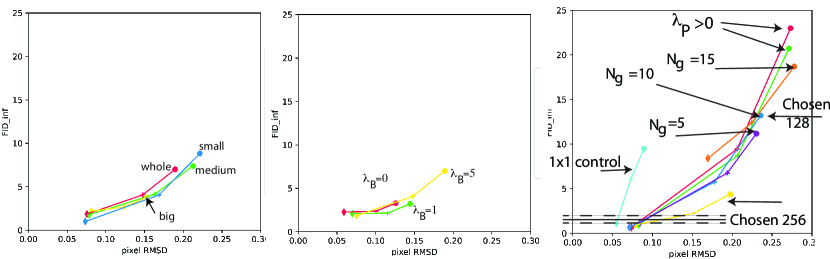
Figure 7: 1 ${\mbox{FID}_{\infty}}$ against MSD for various parameter choices for model selection. Left: PatchGAN adversary scale affects performance; the small receptive field is best. Center: $\lambda_{B}$ encourages variations without much adverse affect on ${\mbox{FID}_{\infty}}$; we chose $\lambda_{B}=5$. Right: $\lambda_{P}>0$ reliably produces more speculative models with weaker FID; the figure is Figure 4 from paper, for reference.

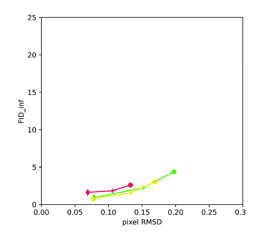
Figure 8: Averaging for equivariance during inference hurts metrics. ${\mbox{FID}_{\infty}}$ against MSD for red: 256x256 images relighted using averaging at inference time; green: relighted 256x256 square crops; yellow: 256x256 square crops from averaged images.

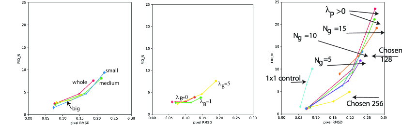
Figure 9: No major effects result from using FID rather than ${\mbox{FID}_{\infty}}$. FID against MSD for various parameter choices for model selection. Left: PatchGAN adversary scale affects performance; the small receptive field is best. Center: $\lambda_{B}$ encourages variations without much adverse affect on ${\mbox{FID}_{\infty}}$; we chose $\lambda_{B}=5$. Right: $\lambda_{P}>0$ reliably produces more speculative models with weaker FID. Compare Fig. 7.

Equivariance: A function $\phi:{\bf x}\in X\rightarrow{\bf y}\in Y$ is equivariant under the action of a group $G$ if there are actions of $G$ on $X$ and $Y$ such that $\phi(g\circ{\bf x})=g\circ\phi({\bf x})$. Information being gained or lost at the boundary is an obstacle to applying the theory of group actions exactly (except for certain finite groups [62]). If one relaxes the definition to require only an approximate match, well-known visual feature representations tend to have strong equivariance properties either by design or in practice [63]. Imposing equivariance properties on intrinsic image decompositions (albedo at a point should not depend on image crop) shows sharp improvements [1]. Relighting has a form of equivariance property: small movements of the camera frame should not affect the overall relighting of a scene (apart from rows and columns of the image moving in and out of view). We use that paper’s crude averaging strategy because we know no better. In this approach we: pad an image; estimate multipliers for a number of closely overlapping crops of the padded image; average overlapping estimates to obtain final multipliers. Doing so reliably loses both MSD and ${\mbox{FID}_{\infty}}$, for reasons we do not know (Figure 8).

Pixel uniformity loss: We expect there is some lighting that makes any location look bright (meaning the image value at each location should be bright), and that any location might be in darkness (meaning that the shading value at each location might be dark). Write $\uparrow{M_{V}I_{V}}$ for the largest value at each location over all generators of $M_{V}I_{V}$ and $\downarrow{M_{V}S_{V}}$ for the smallest value at each location over all generators of $M_{V}S_{V}$. We use:

$${\cal L}_{P}(I_{V};\phi)=\overline{E}$$

where

$$E=\left[-\mbox{min}(0.95-\uparrow{M_{V}I_{V}},0)+\mbox{max}(\downarrow{M_{V}S_{V}}-0.05,0)\right]$$

Pixel uniformity loss reliably produces more speculative models with weaker ${\mbox{FID}_{\infty}}$ (Figure 7).

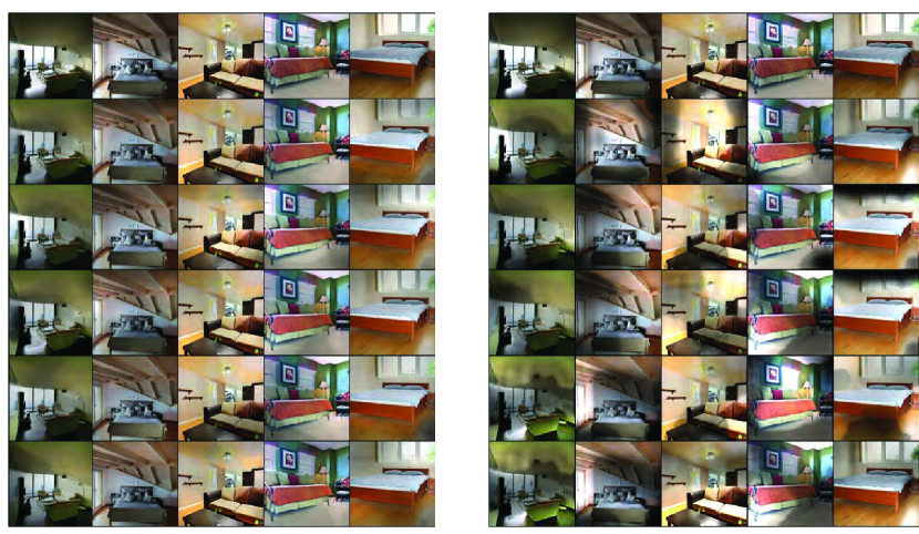
Figure 11: Images relighted at $\alpha=0.5$ left, less variable and $\alpha=0.01$, much more variable right. At $\alpha=0.5$ images have higher quality, but tend to be less variable. At $\alpha=0.01$, the difficulties presented by extrapolation become more obvious.

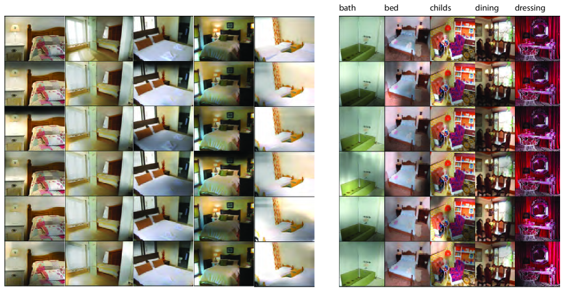
Figure 12: Our method produces qualitative changes in the distribution of light, and appears to generalize well across datasets. Left: Further qualitative results on LSUN-Bedrooms; Right: Results for the first image each of the validation set for 10 scenes with “room” in their name from the PlacesRooms dataset; relights are not curated. Top: Image; other: relights obtained using our method, $\alpha=0.5$. All relights are shown at the same mean intensity as the original image, to ensure that effects are not masked by overall shift in brightness.

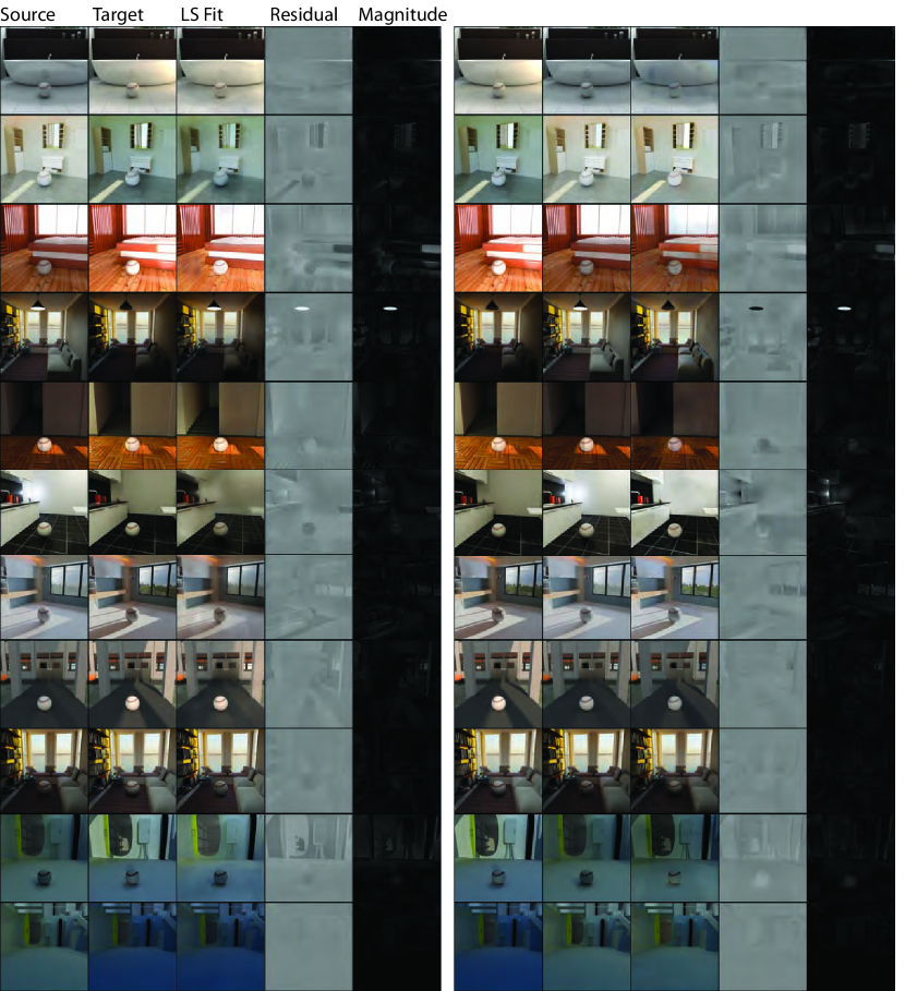
Figure 13: We show all pairs of source/target/least-squares images used to prepare Figure 5 of the main paper. Recall that shows results of: rendering CGI scenes under two lights; computing the multipliers for the source; constructing weighted sum of multipliers that yields a least squares fit to the target; then comparing target to the least squares. The residual error in intensity is shown on a scale where white is 1; mid grey is 0; and black is -1. Note relatively good fits, suggesting that for the cases we have investigated, multipliers are a reasonable fit. Quantitative: over a total of 11 pairs (22 tests), for a dataset we will provide, we find average metrics between the least squares prediction and the target of RMSD: 0.0503 PSNR: 26.6 LPIPS: 0.0648, suggesting quite successful prediction of the target by source multipliers.

9 Appendix II: Proof of Theorem 1

We wish to compare the radiosity of a scene with that of a similar scene, of somewhat different geometry, albedo and luminaire. The key result is the difference between these two radiosities can be described in a sensible way, and can be bounded. In turn, it follows that sufficiently similar scenes will share generators.

9.1 Notation

It is enough to work with a simplified model of a scene $V$ as a tuple $({\cal G},\rho,E)$ of geometry, albedo and luminaire (rather than stochastic family of luminaires). ${\cal G}$ consists of a set of surfaces parametrized in some way and a 2D domain for that parametrization; write ${\cal G}=({{\bf s}}({{\bf x}}),{\cal D})$. Significant complications in the analysis can occur associated with concave “creases” or at surface interpenetrations. These complications aren’t physically important – every corner in a room is made smooth by at least a thin layer of paint or dirt – and so we avoid them by assuming:

• ${\cal D}$ is compact (but need not be connected) with finite area.

• Each connected component of ${\cal D}$ represents a distinct surface.

• Surfaces are parametrized by ${{\bf s}}({{\bf x}})$, where ${{\bf s}}$ is at least $C^{1}$ and is an embedding (surfaces do not self-intersect).

• Surfaces are orientable, and are oriented.

• For any pair of points ${{\bf x}}$, ${{\bf y}}$, we have $k({{\bf x}},{{\bf y}})\leq C$ for some large finite constant $C$ and $k$ defined below. This rules out “throats” – places where the gap between surfaces narrows and then opens out, Figure 14 – in the geometry, and bounds the largest curvatures. Larger $C$ corresponds to narrower throats and tighter curvatures being allowed. The condition is sufficient to ensure the kernel is compact, below.

Note that parametrizing surfaces by atlases of charts complicates notation without changing the analysis; we will suppress these details. Write

$${{\mid\!\mid\!{E}\!\mid\!\mid}_{p}}=\left[\int_{\cal D}E^{p}d{{\bf x}}\right]^{1/p}$$

($1\leq p\leq\infty$) for the $p$ norm of $E$. Recall that for an operator ${\bf K}$

$${{\mid\!\mid\!{{\bf K}}\!\mid\!\mid}_{p}}\leq{\mid\!\mid\!{{\bf K}}\!\mid\!\mid_{\infty}}^{\frac{(p-1)}{p}}{\mid\!\mid\!{{\bf K}}\!\mid\!\mid}_{1}^{\frac{1}{p}}$$

(eg [40], [64] p.144 or [65] p.518). All operators here will have both ${\mid\!\mid\!{{\bf K}}\!\mid\!\mid}_{1}<1$ and ${\mid\!\mid\!{{\bf K}}\!\mid\!\mid_{\infty}}<1$, so that results apply for any $p$; we write ${\mid\!\mid\!{{\bf K}}\!\mid\!\mid}$.

We wish to compare the radiosity $B_{V}$ of a scene $V$ with the radiosity $B_{V}^{\prime}$ of a similar scene $V^{\prime}$. These scenes have somewhat different geometry, albedo and luminaire. We consider affine transformations of the geometry, so that ${\cal G}^{\prime}({\cal G},{{\cal A}},{{\bf b}})=({{\cal A}}{{\bf s}}({{\bf x}})+{{\bf b}},{\cal D})$. We will prove:

Theorem 1: For $V=({\cal G},\rho,E)$ and $V^{\prime}=({\cal G}^{\prime}({\cal G},{{\cal A}},{{\bf b}}),\rho^{\prime},E^{\prime})$, where $\epsilon_{E}{\mid\!\mid\!{E}\!\mid\!\mid}={\mid\!\mid\!{E-E^{\prime}}\!\mid\!\mid}$, $\epsilon_{\rho}=\mbox{sup}_{\cal D}{\mbox{abs}{{\left[\rho-\rho^{\prime}\right]}}}$, $p=\mbox{sup}_{\cal D}\rho$, $p^{\prime}=\mbox{sup}_{\cal D}\rho^{\prime}$, $c$ is the condition number of ${{\cal A}}$ (ratio of largest to smallest eigenvalues), we have:

$${\mid\!\mid\!{B_{V}-B_{V^{\prime}}}\!\mid\!\mid}\leq\left[\begin{array}[]{c}\frac{\epsilon_{E}}{1-p}+\\ \left[\frac{\epsilon_{\rho}(1+\epsilon_{E})}{(1-p)(1-p^{\prime})}\right]+\\ \frac{(c^{4}-1)(1+\epsilon_{E})}{(1-p^{\prime})^{2}}\end{array}\right]{\mid\!\mid\!{E}\!\mid\!\mid}$$

9.2 Standard results

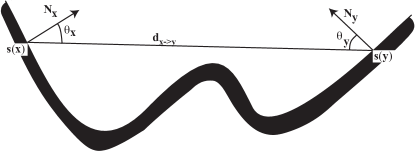
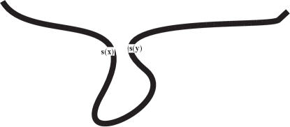
Figure 14: Left: Our notation. Right: a throat.

The geometry consists of a set of parametrized surfaces. Write ${\cal D}$ for the domain of the parametrization. For a parameter vector ${{\bf x}}\in{\cal D}$ write ${{\bf s}}({{\bf x}})$ for the corresponding surface point; $B({{\bf x}})$ for radiosity at that point; $\rho({{\bf x}})$ for the albedo at that point; $E({{\bf x}})$ for the radiant exitance at that point; $V({{\bf x}},{{\bf y}})$ for the visibility function that is $1$ when there is a direct line of sight from ${{\bf s}}({{\bf x}})$ to ${{\bf s}}({{\bf x}})$ and 0 otherwise; ${{\bf d}}_{{{\bf x}}\rightarrow{{\bf y}}}={{\bf s}}({{\bf y}})-{{\bf s}}({{\bf x}})$; and ${{\bf N}}({{\bf x}})$ for a unit normal at ${{\bf x}}$. Figure 14 shows some notation commonly used. Standard diffuse interreflection theory (see, eg [50, 66, 52, 53]) gives

$$B({{\bf x}})=E({{\bf x}})+\rho({{\bf x}})\int_{\cal D}k({{\bf x}},{{\bf y}})B({{\bf y}})dA_{{{\bf y}}}$$

where

$$k({{\bf x}},{{\bf y}}) = \frac{1}{\pi}\frac{V({{\bf x}},{{\bf y}})\cos\theta_{{{\bf x}}}\cos\theta_{{{\bf y}}}}{{\mid\!\mid\!{{{\bf d}}_{{{\bf x}}\rightarrow{{\bf y}}}}\!\mid\!\mid^{2}_{2}}}$$

      (notation in Figure 14)

$$= \frac{V({{\bf x}},{{\bf y}})\left[{{\bf N}}^{T}({{\bf x}}){{\bf d}}_{{{\bf x}}\rightarrow{{\bf y}}}\right]\left[{{\bf N}}^{T}({{\bf y}}){{\bf d}}_{{{\bf y}}\rightarrow{{\bf x}}}\right]}{\left[{{\bf d}}^{T}_{{{\bf x}}\rightarrow{{\bf y}}}{{\bf d}}_{{{\bf x}}\rightarrow{{\bf y}}}\right]^{2}}$$

(recalling ${{\bf N}}$ is a unit normal). Write ${\bf D}_{\rho}$ for the linear operator that maps $f({{\bf x}})$ to $(\rho f)({{\bf x}})$. We can now abbreviate into $B=E+{\bf D}_{\rho}{\bf T}B=E+{\bf K}B$, where ${\bf D}_{\rho}$, ${\bf T}$ and ${\bf K}$ are linear integral operators. It is known that

$${\mid\!\mid\!{{\bf T}}\!\mid\!\mid}\leq 1$$

(for example, our ${\bf T}$ is the ${\bf K}{\bf G}$ of [40], sec 5.3, with constant diffuse BRDF of $1$). Furthermore, writing

$$p={\mid\!\mid\!{\rho({{\bf x}})}\!\mid\!\mid_{\infty}}<1$$

we have

$${\mid\!\mid\!{{\bf D}_{\rho}}\!\mid\!\mid}\leq p$$

by simple calculation and so

$${\mid\!\mid\!{{\bf K}}\!\mid\!\mid}\leq p.$$

For our assumptions,

$$\int_{\cal D}\int_{\cal D}\mid\!k({{\bf x}},{{\bf y}})\!\mid^{2}dA_{{{\bf x}}}dA_{{{\bf y}}}\leq C^{2}\mbox{Area(${\cal D})$}^{2},$$

so that $k$ is a Hilbert-Schmidt kernel. Because the kernel is Hilbert-Schmidt, ${\bf K}$ is a compact operator (eg [67]). There is then a Neumann series solution

$$B = {\bf M}^{-1}E$$

$$= E+{\bf K}E+{\bf K}^{2}E+\ldots$$

$$= \mbox{exitance}+\mbox{one bounce}+\mbox{two bounces}+\ldots$$

which converges for all $r<1$ (and so all practical scenes). It follows that

$${\mid\!\mid\!{{\bf M}^{-1}}\!\mid\!\mid}\leq\frac{1}{1-p}$$

9.3 Lemma 1: Perturbed Luminaire

Assume that the luminaires for $V^{\prime}$ differ from those of $V$ (but geometry and albedo are the same), so $V=({\cal G},\rho,E)$ and $V^{\prime}=({\cal G},\rho,E^{\prime})$. Standard results yield:

Lemma 1: using the notation above

$${\mid\!\mid\!{B_{V}-B_{V^{\prime}}}\!\mid\!\mid}\leq\frac{1}{1-p}{\mid\!\mid\!{E-E^{\prime}}\!\mid\!\mid}=\frac{\epsilon_{E}}{1-p}{\mid\!\mid\!{E}\!\mid\!\mid}.$$

Proof: ${\mid\!\mid\!{{\bf M}^{-1}}\!\mid\!\mid}$ is bounded by $\frac{1}{1-p}$, above. $\square$

9.4 Lemma 3: Perturbed Albedo

Now assume that $V=({\cal G},\rho,E)$ and $V^{\prime}=({\cal G},\rho^{\prime},E)$ and $\rho^{\prime}=\rho+\delta$. Write $\epsilon_{\rho}={\mid\!\mid\!{{\bf D}_{\delta}}\!\mid\!\mid}$. We expect $B^{\prime}$ to differ from $B_{V}$ because it contains multiple bounce terms (above). For example, the shading in a very dark room is notably different from that in a very light room (eg [50, 66, 68]), because low albedos mean that the multiple bounce terms are very small. Equivalently ${\bf M}$ and ${\bf M}^{\prime}$ are different. However, ${\bf G}$ is bounded and we have ${\mid\!\mid\!{{\bf M}}\!\mid\!\mid}=p\leq 1$ and ${\mid\!\mid\!{{\bf M}^{\prime}}\!\mid\!\mid}=p^{\prime}\leq 1$. The dynamic range of practical albedos is quite limited (eg [69]), so it is reasonable to bound $\rho({{\bf x}})$ away from both 0 and 1.

Lemma 2: using the notation above, for all pairs of $0<\epsilon\leq\rho\leq(1-\epsilon)<1$ and $0<\epsilon\leq\rho^{\prime}\leq(1-\epsilon)<1$, ${\mid\!\mid\!{{\bf D}_{\rho-\rho^{\prime}}}\!\mid\!\mid}=\epsilon_{\rho}<1$

Proof: for some test function $f$,

$${\bf D}_{\rho-\rho^{\prime}}f=(\rho({{\bf x}})-\rho^{\prime}({{\bf x}}))f({{\bf x}}).$$

Then

$${\mid\!\mid\!{{\bf D}_{\rho-\rho^{\prime}}f}\!\mid\!\mid_{1}} = \int_{\cal D}\mid\!(\rho({{\bf x}})-\rho^{\prime}({{\bf x}}))f({{\bf x}})\!\mid dA_{{{\bf x}}}$$

$$\leq \int_{\cal D}\mid\!(\rho({{\bf x}})-\rho^{\prime}({{\bf x}}))\!\mid\mid\!f({{\bf x}})\!\mid dA_{{{\bf x}}}$$

$$\leq {\begin{array}[]{c}\mbox{sup}\\ {{{\bf x}}}\end{array}}\left[\mid\!(\rho({{\bf x}})-\rho^{\prime}({{\bf x}}))\!\mid\right]\int\mid\!f({{\bf x}})\!\mid dA_{{{\bf x}}}.$$

The constraints on $\rho$, $\rho^{\prime}$ ensure

$$\sup{{{\bf x}}}\left[\mid\!(\rho({{\bf x}})-\rho^{\prime}({{\bf x}}))\!\mid\right]<1$$

and ${\mid\!\mid\!{{\bf D}_{\rho-\rho^{\prime}}}\!\mid\!\mid_{\infty}}<1$, so the result follows for all norms. $\square$

This yields the novel (but fairly straightforward)

Lemma 3: using the notation above

$${\mid\!\mid\!{B_{V^{\prime}}-B_{V}}\!\mid\!\mid}\leq\left[\frac{1}{1-p}\right]\left[\frac{1}{1-p^{\prime}}\right]\epsilon_{\rho}{\mid\!\mid\!{E}\!\mid\!\mid}$$

Proof: We have $(I-{\bf D}_{\rho}{\bf G})B_{V}=E=(I-{\bf D}_{(\rho+\delta)}{\bf G})B_{V^{\prime}}$, so

$$B_{V^{\prime}}-B_{V} = {\bf D}_{\rho^{\prime}}{\bf G}B_{V^{\prime}}-{\bf D}_{\rho}{\bf G}B_{V}$$

$$= {\bf D}_{\rho^{\prime}}{\bf G}B_{V}-{\bf D}_{\rho}{\bf G}B_{V}+{\bf D}_{\rho^{\prime}}{\bf G}(B_{V^{\prime}}-B_{V})$$

$$= {\bf D}_{\delta}{\bf G}B_{V}+{\bf D}_{\rho^{\prime}}{\bf G}(B_{V^{\prime}}-B_{V})$$

$$= {\bf D}_{\delta}{\bf G}{\bf M}^{-1}E+{\bf D}_{\rho^{\prime}}{\bf G}(B_{V^{\prime}}-B_{V})$$

so

$$B_{V^{\prime}}-B_{V}={\bf M}^{\prime-1}{\bf D}_{\delta}{\bf G}{\bf M}^{-1}E.$$

Now ${\mid\!\mid\!{{\bf D}_{\delta}{\bf G}}\!\mid\!\mid}\leq\epsilon_{\rho}$, so

$${\mid\!\mid\!{B_{V^{\prime}}-B_{V}}\!\mid\!\mid} = {\mid\!\mid\!{{\bf M}^{\prime-1}{\bf D}_{\delta}{\bf G}{\bf M}^{-1}E}\!\mid\!\mid}$$

$$\leq \left[\frac{1}{1-p}\right]\left[\frac{1}{1-p^{\prime}}\right]\epsilon_{\rho}{\mid\!\mid\!{E}\!\mid\!\mid}$$

$\square$

9.5 Theorem 1: Perturbed Geometry

We wish to study the effect of small changes in geometry on the solution $B$. We have found no results on the effect of perturbing geometry, which appear to be hard to obtain (cf [43], p176 says they are; [44] estimate the effect of flat ports on an integrating sphere).

Small geometric changes can produce major changes in visibility which are difficult to bound. We consider affine transformations of the surfaces, so that ${{\bf s}}({{\bf x}})$ is mapped to ${\cal T}({{\bf s}})={{\cal A}}{{\bf s}}({{\bf x}})+{{\bf b}}$ ($\mbox{det}({{\cal A}})\geq 0$). We assume that the smallest singular value of ${{\cal A}}$ is positive. There are two advantages of this model: first, it is a reasonable description of small changes between otherwise quite similar rooms (small anisotropic scalings in the right coordinate system); second, the visibility function for ${\cal T}({{\bf s}})$ is the same as the visibility function for ${{\bf s}}$ (lemma 4, below).

9.5.1 Transformations and Functions

The transformation produces a natural bijection between functions of original and transformed geometry. This is so natural that it can be difficult to see at first glance. Assume we have a function $f$ defined on the first geometry. We must know the value that $f$ takes at each point on the geometry, which means we know the value at each point in the parameter space. But this parameter space parametrizes the transformed geometry, too, so we have a corresponding function on the transformed geometry (this argument yields that the mapping between function spaces is a bijection). For $f$ a function defined on the original parametrization, write ${\cal T}(f)$ for the transformed version.

This natural correspondence may not respect the geometric transformation on the embedded surfaces. This means we need to distinguish between a function mapped through the correspondence and one evaluated on the new geometry. For example, consider the function $\mbox{sqdist}({{\bf x}}_{0},{{\bf x}}_{1})={\mid\!\mid\!{{{\bf s}}({{\bf x}}_{0})-{{\bf s}}({{\bf x}}_{1})}\!\mid\!\mid^{2}_{2}}$. If ${{\cal A}}=2*Id$, the distance between points on the transformed geometry has doubled. Write $\mbox{sqdist}^{\prime}({{\bf x}}_{0},{{\bf x}}_{1})={\mid\!\mid\!{{{\cal A}}{{\bf s}}({{\bf x}}_{0})-{{\cal A}}{{\bf s}}({{\bf x}}_{1})}\!\mid\!\mid^{2}_{2}}$ (the prime indicates the function is evaluated on the transformed geometry). We have ${\cal T}(\mbox{sqdist})({{\bf x}}_{0},{{\bf x}}_{1})=(1/4){\mid\!\mid\!{{{\cal A}}{{\bf s}}({{\bf x}}_{0})-{{\cal A}}{{\bf s}}({{\bf x}}_{1})}\!\mid\!\mid^{2}_{2}}=(1/4)\mbox{sqdist}^{\prime}({{\bf x}}_{0},{{\bf x}}_{1})$.

9.5.2 Transformations and the Kernel

A similar natural correspondence applies to operators. We must now consider the relationship between ${\cal T}({\bf K})$ and ${\bf K^{\prime}}$. Each is a bounded linear operator defined on functions of ${\cal G}^{\prime}$, but they are different. ${\cal T}({\bf K})$ is obtained by applying the natural correspondence to ${\cal K}$; in contrast ${\cal K}^{\prime}$ is obtained by computing the kernel using the geometry of ${\cal G}^{\prime}$, which may give a different operation.

By tracking the effects of affine transformations on the terms of $k$, we can constrain the difference. First, we have

Lemma 4: $V({{\bf x}},{{\bf y}})={\cal T}(V({{\bf x}},{{\bf y}}))=V^{\prime}({{\bf x}},{{\bf y}})$

Proof: The main issue is keeping track of notation; the first equality is obvious (natural correspondence); the second – that computing the view function in the transformed space is equivalent to computing it in the original space, and mapping through correspondence – follows because affine transformations map lines to lines and preserve incidence. $\square$

We must now investigate how $k$ transforms. We have:

Lemma 5: ${{\bf N}}^{\prime}({{\bf x}})=\frac{{{\cal A}}^{-T}{{\bf N}}_{{{\bf x}}}}{\sqrt{{{\bf N}}^{T}{{\cal A}}^{-1}{{\cal A}}^{-T}{{\bf N}}}}$

Proof: Write $\Pi_{{{\bf x}}}$ for the tangent plane at ${{\bf x}}$. For ${{\bf u}}\in\Pi_{{{\bf x}}}$, we have for non-unit normal ${{\bf n}}$, ${{{\bf n}}}({{\bf x}})^{T}({{\bf u}}-{{\bf x}})=0$. But ${{\bf u}}$ transforms to ${{\cal A}}{{\bf u}}+{{\bf b}}$, etc. and we must have ${{\bf n}}^{\prime}({{\bf x}})^{T}\left({{\cal A}}({{\bf u}}-{{\bf x}})\right)=0$, and the result follows by requiring the normal be a unit normal; equivalently, normals are covariant. $\square$

Write $\sigma_{x}$ for the largest singular value of ${{\cal A}}$, $\sigma_{n}$ for the smallest (which is positive), and $c=\frac{\sigma_{x}}{\sigma_{n}}$ for the condition number. We have

Lemma 6: $(\sigma_{n}){{\bf N}}^{T}{{\bf d}}_{{{\bf u}}\rightarrow{{\bf v}}}\leq{{\bf N}}^{\prime T}{{\bf d}}^{\prime}_{{{\bf u}}\rightarrow{{\bf v}}}\leq({\sigma_{x}}){{\bf N}}^{T}{{\bf d}}_{{{\bf u}}\rightarrow{{\bf v}}}$

Proof: ${{\bf N}}^{\prime T}{{\bf d}}^{\prime}_{{{\bf u}}\rightarrow{{\bf v}}}=\frac{{{\bf N}}^{T}{\bf A}^{-1}{\bf A}{{\bf d}}_{{{\bf u}}\rightarrow{{\bf v}}}}{\sqrt{{{\bf N}}^{T}{\bf A}^{-1}{\bf A}^{-T}{{\bf N}}}}$ and the bound follows. $\square$

Lemma 7: ${\sigma_{n}}^{2}{\cal T}(dA_{{{\bf y}}})\leq dA^{\prime}_{{{\bf y}}}\leq{\sigma_{x}}^{2}{\cal T}(dA_{{{\bf y}}})$.

Proof: $dA^{\prime}_{{{\bf y}}}$ is the infinitesimal area spanned by two infinitesimal vectors $dx_{1}$ and $dx_{2}$. The largest (resp. smallest) scaling of each length is by the largest (resp. smallest) singular value of ${{\cal A}}$. $\square$

We then obtain the novel:

Lemma 8: For affine transformations, $c^{-4}{\bf K}({\cal T}(f))\leq{\bf K}^{\prime}({\cal T}(f))\leq c^{4}{\bf K}({\cal T}(f))$ for any $f_{{{\bf s}}}$

Proof: For any two vectors ${{\bf u}}^{\prime T}{{\bf v}}^{\prime}={{\bf u}}^{T}{{\cal A}}^{T}{{\cal A}}{{\bf v}}$. Then $\sigma^{2}_{n}{{\bf u}}^{T}{{\bf v}}\leq{{\bf u}}^{T}{{\cal A}}^{T}{{\cal A}}{{\bf v}}={{\bf u}}^{\prime T}{{\bf v}}^{\prime}\leq\sigma^{2}_{x}{{\bf u}}^{T}{{\bf v}}$. Lemma 6 deals with the angles. Write

$${\bf K^{\prime}}({\cal T}(f))=\int_{\cal D}k^{\prime}({{\bf x}},{{\bf y}})f({{\bf y}})dA^{\prime}_{{{\bf y}}}$$

where

$$k^{\prime}({{\bf x}},{{\bf y}})=\frac{V^{\prime}({{\bf x}},{{\bf y}})\left[{{\bf N}}^{\prime T}({{\bf x}}){{\bf d}}^{\prime}_{{{\bf x}}\rightarrow{{\bf y}}}\right]\left[{{\bf N}}^{\prime T}({{\bf y}}){{\bf d}}^{\prime}_{{{\bf y}}\rightarrow{{\bf x}}}\right]}{\left[{{\bf d}}^{\prime T}_{{{\bf x}}\rightarrow{{\bf y}}}{{\bf d}}^{\prime}_{{{\bf x}}\rightarrow{{\bf y}}}\right]^{2}}$$

But

$$\left[\begin{array}[]{c}\left[({\sigma_{n}}){{\bf N}}^{T}({{\bf x}}){{\bf d}}_{{{\bf x}}\rightarrow{{\bf y}}}\right]\times\\ \left[({\sigma_{n}}){{\bf N}}^{T}({{\bf y}}){{\bf d}}_{{{\bf y}}\rightarrow{{\bf x}}}\right]\times\\ \left[\sigma^{2}_{n}dA_{{{\bf y}}}\right]\end{array}\right] \leq \left[\begin{array}[]{c}\left[{{\bf N}}^{\prime T}({{\bf x}}){{\bf d}}^{\prime}_{{{\bf x}}\rightarrow{{\bf y}}}\right]\times\\ \left[{{\bf N}}^{\prime T}({{\bf x}}){{\bf d}}^{\prime}_{{{\bf y}}\rightarrow{{\bf x}}}\right]\times\\ dA^{\prime}_{{{\bf y}}}\end{array}\right]$$

$$\leq \left[\begin{array}[]{c}\left[({\sigma_{x}}){{\bf N}}^{T}({{\bf x}}){{\bf d}}_{{{\bf x}}\rightarrow{{\bf y}}}\right]\times\\ \left[({\sigma_{x}}){{\bf N}}^{T}({{\bf y}}){{\bf d}}_{{{\bf y}}\rightarrow{{\bf x}}}\right]\times\\ \left[\sigma^{2}_{x}dA_{{{\bf y}}}\right]\end{array}\right]$$

and

$$\sigma_{n}^{4}\left[{{\bf d}}^{T}_{{{\bf x}}\rightarrow{{\bf y}}}{{\bf d}}_{{{\bf x}}\rightarrow{{\bf y}}}\right]^{2} \leq \left[{{\bf d}}^{\prime T}_{{{\bf x}}\rightarrow{{\bf y}}}{{\bf d}}^{\prime}_{{{\bf x}}\rightarrow{{\bf y}}}\right]^{2}$$

$$= \left[{{\bf d}}^{T}_{{{\bf x}}\rightarrow{{\bf y}}}{{\cal A}}^{T}{{\cal A}}{{\bf d}}_{{{\bf x}}\rightarrow{{\bf y}}}\right]^{2}$$

$$\leq \sigma_{x}^{4}\left[{{\bf d}}^{T}_{{{\bf x}}\rightarrow{{\bf y}}}{{\bf d}}_{{{\bf x}}\rightarrow{{\bf y}}}\right]^{2}$$

so that

$$c^{-4}{\cal T}({\bf K})({\cal T}(f)) = \int_{\cal D}\frac{\sigma_{n}^{4}}{\sigma_{x}^{4}}k({{\bf x}},{{\bf y}})f({{\bf y}})dA_{{{\bf y}}}$$

$$\leq \int_{\cal D}k^{\prime}({{\bf x}},{{\bf y}})f({{\bf y}})dA^{\prime}_{{{\bf y}}}$$

$$\leq \int_{\cal D}\frac{\sigma_{x}^{4}}{\sigma_{n}^{4}}k({{\bf x}},{{\bf y}})f({{\bf y}})dA_{{{\bf y}}}$$

$$= c^{4}{\cal T}({\bf K})({\cal T}(f))$$

$\square$.

which leads to

Lemma 9: With the notation above,

$${\mid\!\mid\!{B_{V}-B_{V^{\prime}}}\!\mid\!\mid}\leq\frac{(c^{4}-1)}{(1-p)^{2}}{\mid\!\mid\!{E}\!\mid\!\mid}$$

Proof:

$$B_{V^{\prime}}-B_{V} = \left({\cal T}(E)-E\right)+\left({\bf K}^{\prime}B_{V^{\prime}}-{\bf K}B_{V}\right)$$

$$= {\bf K}^{\prime}B_{V^{\prime}}-{\bf K}^{\prime}B_{V}+{\bf K}^{\prime}B_{V}-{\bf K}B_{V}$$

(recall $${\cal T}(E)=E$$)

$$= {\bf K}^{\prime}(B_{V^{\prime}}-B_{V})+{\bf K}^{\prime}B_{V}-{\bf K}B_{V}$$

so that

$$\left({\bf I}-{\bf K}^{\prime}\right)\left(B_{V^{\prime}}-B_{V}\right)=\left({\bf K}^{\prime}-{\bf K}\right)B_{V}$$

and

$$\left(B_{V^{\prime}}-B_{V}\right)={\bf M}^{\prime-1}\left({\bf K}^{\prime}-{\bf K}\right)B_{V}.$$

Notice that the kernel is everywhere non-negative, and for every point ${{\bf x}}$ and for any non-negative function $f$, we have $0\leq({\bf K}f)(x)$. Since $E$ is non-negative, so is $B_{V}$. From lemma 6, for non-negative $f$, we have $({\bf K}^{\prime}f)({{\bf x}})\leq c^{4}({\bf K}f)({{\bf x}})$ at every point ${{\bf x}}$, so that ${\bf K}^{\prime}f-{\bf K}f\leq(c^{4}-1){\bf K}f$ at every point. This means

$${\mid\!\mid\!{\left(B_{V^{\prime}}-B_{V}\right)}\!\mid\!\mid} = {\mid\!\mid\!{{\bf M}^{\prime-1}\left({\bf K}^{\prime}-{\bf K}\right)B_{V}}\!\mid\!\mid}$$

$$\leq \frac{1}{(1-p^{\prime})}{\mid\!\mid\!{\left({\bf K}^{\prime}-{\bf K}\right)B_{V}}\!\mid\!\mid}$$

$$\leq \frac{1}{(1-p^{\prime})}(c^{4}-1){\mid\!\mid\!{B_{V}}\!\mid\!\mid}$$

$$\leq \frac{1}{(1-p^{\prime})}(c^{4}-1)\frac{1}{(1-p)}{\mid\!\mid\!{E}\!\mid\!\mid}$$

$$= \frac{(c^{4}-1)}{(1-p)^{2}}{\mid\!\mid\!{E}\!\mid\!\mid}$$

where the last step works because $p^{\prime}=p$, because $\rho^{\prime}={\cal T}(\rho)=\rho$. $\square$.

Finally, we can prove the entirely novel

Theorem 1: For $V=({\cal G},\rho,E)$ and $V^{\prime}=({\cal G}^{\prime}({\cal G},{{\cal A}},{{\bf b}}),\rho^{\prime},E^{\prime})$, where $\epsilon_{E}{\mid\!\mid\!{E}\!\mid\!\mid}={\mid\!\mid\!{E-E^{\prime}}\!\mid\!\mid}$, $\epsilon_{\rho}=\mbox{sup}_{\cal D}{\mbox{abs}{{\left[\rho-\rho^{\prime}\right]}}}$, $p=\mbox{sup}_{\cal D}\rho$, $p^{\prime}=\mbox{sup}_{\cal D}\rho^{\prime}$, $c$ is the condition number of ${{\cal A}}$ (ratio of largest to smallest eigenvalues), we have:

$${\mid\!\mid\!{B_{V}-B_{V^{\prime}}}\!\mid\!\mid}\leq\left[\begin{array}[]{c}\left[\frac{\epsilon_{E}}{1-p}\right]+\\ \left[\frac{\epsilon_{\rho}(1+\epsilon_{E})}{(1-p)(1-p^{\prime})}\right]+\\ \frac{(c^{4}-1)(1+\epsilon_{E})}{(1-p^{\prime})^{2}}\end{array}\right]{\mid\!\mid\!{E}\!\mid\!\mid}$$

Proof: Write $V_{1}=({\cal G},\rho,E^{\prime})$, $V_{2}=({\cal G},\rho^{\prime},E^{\prime})$. Then

$${\mid\!\mid\!{B_{V}-B_{V^{\prime}}}\!\mid\!\mid}\leq\left[\begin{array}[]{c}{\mid\!\mid\!{B_{V}-B_{V_{1}}}\!\mid\!\mid}+\\ {\mid\!\mid\!{B_{V_{1}}-B_{V_{2}}}\!\mid\!\mid}+\\ {\mid\!\mid\!{B_{V_{2}}-B_{V^{\prime}}}\!\mid\!\mid}\end{array}\right]\mbox{(triangle inequality)}$$

and ${\mid\!\mid\!{E^{\prime}}\!\mid\!\mid}\leq(1+\epsilon_{E}){\mid\!\mid\!{E}\!\mid\!\mid}$ but

$${\mid\!\mid\!{B_{V}-B_{V_{1}}}\!\mid\!\mid} \leq \frac{\epsilon_{E}}{1-p}{\mid\!\mid\!{E}\!\mid\!\mid}\mbox{ (Lemma 1)}$$

$${\mid\!\mid\!{B_{V_{1}}-B_{V_{2}}}\!\mid\!\mid} \leq \frac{\epsilon_{\rho}}{(1-p)(1-p^{\prime})}{\mid\!\mid\!{E^{\prime}}\!\mid\!\mid}\mbox{ (Lemma 3)}$$

$$\leq \frac{\epsilon_{\rho}}{(1-p)(1-p^{\prime})}(1+\epsilon_{E}){\mid\!\mid\!{E}\!\mid\!\mid}\mbox{ (definitions)}$$

$${\mid\!\mid\!{B_{V_{2}}-B_{V^{\prime}}}\!\mid\!\mid} \leq \frac{(c^{4}-1)}{(1-p^{\prime})^{2}}(1+\epsilon_{E}){\mid\!\mid\!{E}\!\mid\!\mid}\mbox{ (Lemma 9)}$$

$\square$

10 Appendix III: Proof of Theorem 2

We now establish that viewing shading fields for a set of similar scenes $V_{i}$ is enough to estimate a representation of the generators for a given scene $V$. It is important to have a representation of the probability that a scene will be illuminated in some particular way. We use the general definition of a scene, above. A scene $V$ is a tuple of geometry, albedo and luminaire model; write $V=\left({\cal G},\rho,{\cal E}\right)$, where ${\cal E}$ is the luminaire model. The geometry ${\cal G}$ consists of a set of surfaces parametrized in some way and a 2D domain for that parametrization; write ${\cal G}=({{\bf s}}({{\bf x}}),{\cal D})$. The luminaire model captures the idea that lighting in a particular scene may change. We have ${\cal E}=\left(E_{1},\ldots E_{N_{e}},P(\theta)\right)$ for a set of potentially many basis luminaires and a probability distribution over the coefficients. This information implies a probability distribution over luminaires for the scene $P(E)$. Two scenes $V$ and $V^{\prime}$ are similar if there is some affine transformation ${\cal A},{{\bf b}}$ ( smallest singular value of ${\cal A}$ greater than zero) such that ${\cal G}^{\prime}({\cal G},{{\cal A}},{{\bf b}})=({{\cal A}}{{\bf s}}({{\bf x}})+{{\bf b}})$ and if ${\cal E}={\cal E}^{\prime}$. Notice this second constraint does not require that the two scenes are lit in the same way, just that the basis of luminaires is the same and the probability distribution over lighting coefficients is the same.

We pass to a finite dimensional representation without loss of generality (to avoid having to deal with function spaces). Choose some $N_{o}$ element orthonormal basis to represent the possible radiosity vectors for the scene (if $N_{o}=N_{e}$, the representation is exact, because there is a finite dimensional space of luminaires). In this basis, any particular radiosity $B({{\bf x}})$ has coefficient vector ${{\bf b}}$. Write $\phi_{i}({{\bf x}})$ for the $i$’th element of the basis; $\Phi=\left[\phi_{1}({{\bf x}}),\ldots,\phi_{N_{o}}({{\bf x}})\right]$; ${{\bf b}}_{i}$ for the coefficient vector representing $B_{i}({{\bf x}})$ (which is the radiosity resulting from $E_{i}({{\bf x}})$); and ${{\cal B}}=\left[{{\bf b}}_{1},\ldots,{{\bf b}}_{N_{e}}\right]$.

For any $r\leq N_{e}$, an effective generator matrix for scene $V$ is the $N_{o}\times r$ matrix ${{\cal G}}_{e,V,r}$ such that for any illumination condition producing radiosity represented by ${{\bf b}}$ , there is some ${{\bf w}}$ such that the radiosity represented by ${{\cal G}}_{e,V,r}{{\bf w}}$ is similar to the actual radiosity field. In particular, we want

$${\cal L}({{\cal G}}_{e,V,r})={{{{\mathbb{E}}}}_{{\theta\sim P(\theta)}}{{\left[{{\mbox{inf}_{{{\bf w}}}{\mid\!\mid\!{{{\cal G}}_{e,V,r}{{\bf w}}-{{\cal B}}\theta}\!\mid\!\mid_{2}}^{2}}}\right]}}}$$

to be small; ${{\cal G}}_{e,V,r}$ is clearly not unique. We choose to have ${{\cal G}}_{e,V,r}$ orthonormal.

Assume we have $k$ radiosity fields $B_{i}$ for a scene under different, unknown, illumination conditions, for $k$ very large. We assume that for the $i$’th field, $\theta_{i}\sim P(\theta)$ (which is not known). We can clearly estimate an effective generator matrix by replacing the expectation with an average. But we do not have $k$ images of the same scene.

Lemma 10: Using the notation above, write

$$C_{{{\bf b}}}={{\cal B}}\left({{{{\mathbb{E}}}}_{{\theta\sim P(\theta)}}{{\left[{{\theta\theta^{T}}}\right]}}}\right){{\cal B}}^{T}.$$

Then:

$${{{{\mathbb{E}}}}_{{\theta\sim P(\theta)}}{{\left[{{\mbox{inf}_{{{\bf w}}}{\mid\!\mid\!{{{\cal G}}_{e,V,r}{{\bf w}}-{{\cal B}}\theta}\!\mid\!\mid_{2}}^{2}}}\right]}}}$$

is equal to

$$\mbox{Tr}\left[C_{{{\bf b}}}\right]-\mbox{Tr}\left[{{\cal G}}_{e,V,r}^{T}C_{{{\bf b}}}{{\cal G}}_{e,V,r}\right]$$

Proof: Manipulation; note that

$$C_{{{\bf b}}}={{{{\mathbb{E}}}}_{{\theta\sim P(\theta)}}{{\left[{{{{\cal B}}\theta\theta^{T}{{\cal B}}^{T}}}\right]}}};$$

that

$${{{{\mathbb{E}}}}_{{\theta\sim P(\theta)}}{{\left[{{\theta^{T}{{\cal B}}^{T}{{\cal B}}\theta}}\right]}}}=\mbox{Tr}\left[C_{{{\bf b}}}\right];$$

and that

$${{{{\mathbb{E}}}}_{{\theta\sim P(\theta)}}{{\left[{{\theta^{T}{{\cal B}}^{T}{{\cal G}}_{e,V,r}{{\cal G}}_{e,V,r}^{T}{{\cal B}}\theta}}\right]}}}=\mbox{Tr}\left[{{\cal G}}_{e,V,r}^{T}C_{{{\bf b}}}{{\cal G}}_{e,V,r}\right].$$

$\square$

We cannot know ${\cal C}_{{{\bf b}}}$, but we do not need to.

Lemma 11: Using the notation above; writing ${{\bf e}}_{i}$ for the eigenvector of $C_{{{\bf b}}}$ corresponding to the $i$’th largest eigenvalue; and assuming that the eigenvalues of $C_{{{\bf b}}}$ are distinct, an optimal value of ${\cal L}({{\cal G}}_{e,V,r})$ is given by

$$\left[{{\bf e}}_{1},\ldots,{{\bf e}}_{r}\right]{{\cal M}}$$

for any $r\times r$ matrix ${{\cal M}}$ of full rank such that ${{\cal M}}^{T}{{\cal M}}=I$

Proof: Follows directly from lemma 10.$\square$

Lemma 12: Using the notation above, and writing $\lambda_{i}$ for the $i$’th largest eigenvalue of $C_{{{\bf b}}}$, the optimal value of ${\cal L}({{\cal G}}_{e,V,r})$ is given by

$$\sum_{i=r+1}^{N_{e}}\lambda_{i}$$

Proof: Follows directly from lemma 10 and 11. $\square$

Assume we collect $N_{s}$ samples of radiosity $\hat{{{\bf b}}}={{\cal B}}\theta$, where $\hat{{{\bf b}}}_{i}$ is the $i$’th such sample, and $\theta\sim P(\theta)$. These yield an estimate of $C_{{{\bf b}}}$, which can be accurate.

Lemma 13: Write $\hat{C}_{{{\bf b}},m}=(1/N_{s})\sum_{i}\hat{{{\bf b}}}_{i}\hat{{{\bf b}}}_{i}^{T}$. Then there is some constant $C_{e}$ such that

$${{{{\mathbb{E}}}}}{{\left[{{\hat{C}_{{{\bf b}},m}-C_{{{\bf b}},m}}}\right]}} = 0$$

and

$${{{{\mathbb{E}}}}}{{\left[{{{\mid\!\mid\!{\hat{C}_{{{\bf b}},m}-C_{{{\bf b}},m}}\!\mid\!\mid_{F}}^{2}}}\right]}} = (1/N_{s})C_{e}$$

Proof: This follows from the weak law of large numbers $\square$

Now collect $N_{s}$ samples of radiosity from different scenes $V_{i}$, each one similar to the scene $V$, where ${{\cal A}}_{i}$ maps the geometry of $V$ to $V_{i}$. Write $\hat{{{\bf b}}}_{i,V_{i}}$ for the $i$’th such sample. Recall that similar scenes have the same basis of luminaires and the same distribution for $\theta$. These samples yield an estimate of $C_{{{\bf b}}}$, too.

Lemma 14: Given ${{\bf b}}$, ${{\bf c}}$, $r$ and $\delta$ such that (a) ${\mid\!\mid\!{{{\bf b}}-{{\bf c}}}\!\mid\!\mid_{2}}\leq\delta$ and (b) ${\mid\!\mid\!{{{\bf b}}}\!\mid\!\mid_{2}}\leq r$, we have:

$${\mid\!\mid\!{{{\bf b}}{{\bf b}}^{T}-{{\bf c}}{{\bf c}}^{T}}\!\mid\!\mid_{F}}\leq 3\delta^{2}r^{2}+4\delta^{3}r+\delta^{4}$$

Proof: Write $\Delta={{\bf c}}-{{\bf b}}$. Then

$${\mid\!\mid\!{{{\bf b}}{{\bf b}}^{T}-{{\bf c}}{{\bf c}}^{T}}\!\mid\!\mid_{F}} = \mbox{Tr}\left[\left({{\bf b}}{{\bf b}}^{T}-{{\bf c}}{{\bf c}}^{T}\right)\left({{\bf b}}{{\bf b}}^{T}-{{\bf c}}{{\bf c}}^{T}\right)^{T}\right]$$

$$= \left(\begin{array}[]{c}({{\bf b}}^{T}{{\bf b}})^{2}\\ -2({{\bf b}}^{T}{{\bf b}}+\Delta^{T}{{\bf b}})^{2}\\ +({{\bf b}}^{T}{{\bf b}}+\Delta^{T}{{\bf b}}+\Delta^{T}\Delta)^{2}\end{array}\right)$$

$$\leq 4\delta r^{3}+3\delta^{2}r^{2}+2\delta^{3}r+\delta^{4}$$

$\square$.

Lemma 15: Write $\hat{C}_{{{\bf b}},m,s}=(1/N_{s})\sum_{i}\hat{{{\bf b}}}_{i,V_{i}}\hat{{{\bf b}}}_{i,V_{i}}^{T}$. Using the notation above, and writing $p=\mbox{max}_{i}\left(\mbox{sup}_{\cal D}\rho_{i}\right)$; $\epsilon_{\rho}=\mbox{max}_{i}\left(\mbox{sup}_{\cal D}{\mbox{abs}{{\left[\rho_{V}-\rho_{V_{i}}\right]}}}\right)$; $c$ for the largest condition number of ${{\cal A}}_{i}$. Write

$$\delta=\left(\frac{\epsilon_{\rho}+(c^{4}-1)}{(1-p)^{2}}\right)\mbox{ and }r=\frac{1}{(1-p)}$$

Then

$${\mid\!\mid\!{\hat{C}_{{{\bf b}},m,s}-C_{{{\bf b}},m}}\!\mid\!\mid_{F}}\leq N_{o}^{2}\left(4\delta r^{3}+3\delta^{2}r^{2}+2\delta^{3}r+\delta^{4}\right)$$

Proof: The $i$’th sample $\theta_{i}$ from $P(\theta)$ yields a luminaire $E$; write $B_{i,V}$ for the resulting radiosity in $V$ and ${{\bf b}}_{i,V}$ for its finite dimensional representation. Theorem 1 yields a bound on ${\mid\!\mid\!{B_{i,V}-B_{i,V_{i}}}\!\mid\!\mid}$, and so on ${\mid\!\mid\!{{{\bf b}}_{i,V}-{{\bf b}}_{i,V_{i}}}\!\mid\!\mid}$. We have ${\mid\!\mid\!{{{\bf b}}_{i,V}-{{\bf b}}_{i,V_{i}}}\!\mid\!\mid}\leq\left(\frac{\epsilon_{\rho}+(c^{4}-1)}{(1-p)^{2}}\right)$. Furthermore, ${\mid\!\mid\!{{{\bf b}}_{i,V}}\!\mid\!\mid}\leq 1/(1-p)$. The result then follows from lemma 14 $\square$.

We can now compute an effective generator matrix $\hat{{{\cal G}}}$ from an estimate ${{\cal C}}_{{{\bf b}},m,s}$ of ${{\cal C}}_{{{\bf b}}}$. This estimate uses observations of multiple similar scenes. The $\hat{{{\cal G}}}$ we obtain from data like this will not be the true ${{\cal G}}$, and we must determine what problems will result from using $\hat{{{\cal G}}}$ (which we can get) in place of ${{\cal G}}$ (which is the true best EGM).

Theorem 2 establishes that using $\hat{{{\cal G}}}$ in place of ${{\cal G}}$ incurs bounded error. Recall the expected error of using ${{\cal G}}$ as the effective generator matrix for estimate ${{\cal C}}$ is

$${\cal L}({{\cal G}};{{\cal C}})=\left(\mbox{Tr}\left[{{\cal C}}\right]-\mbox{Tr}\left[{{\cal G}}^{T}{{\cal C}}{{\cal G}}\right]\right)$$

Now estimate the effective generator matrix using ${{\cal C}}_{{{\bf b}},m,s}$ to obtain

$$\hat{{{\cal G}}}=\begin{array}[]{c}\mbox{argmax}\\ {{\cal G}}|{{\cal G}}^{T}{{\cal G}}=I\end{array}{\cal L}({{\cal G}};{{\cal C}}_{{{\bf b}},m,s})$$

Using $\hat{{{\cal G}}}$ to represent the radiosity of the scene will incur expected error

$${\cal L}(\hat{{{\cal G}}};{{\cal C}}_{{{\bf b}}})=\left(\mbox{Tr}\left[{{\cal C}}_{{{\bf b}}}\right]-\mbox{Tr}\left[\hat{{{\cal G}}}^{T}{{\cal C}}_{{{\bf b}}}\hat{{{\cal G}}}\right]\right).$$

Theorem 2: ${\cal L}(\hat{{{\cal G}}};{{\cal C}}_{{{\bf b}}})-{\cal L}({{\cal G}};{{\cal C}}_{{{\bf b}}})$ is bounded.

Proof:

We have

$${\cal L}(\hat{{{\cal G}}};{{\cal C}}_{{{\bf b}}})-{\cal L}({{\cal G}};{{\cal C}}_{{{\bf b}}})=\mbox{Tr}\left[\hat{{{\cal G}}}^{T}{{\cal C}}_{{{\bf b}}}\hat{{{\cal G}}}\right]-\mbox{Tr}\left[{{\cal{G}}}^{T}{{\cal C}}_{{{\bf b}}}{{\cal{G}}}\right]$$

Recall ${{\cal G}}$ is chosen to minimize ${\cal L}({{\cal G}};{{\cal C}}_{{{\bf b}}})$, and is orthornormal, so will consist of the eigenvectors of ${{\cal C}}_{{{\bf b}}}$ corresponding to the $r$ largest eigenvalues. In turn, $\hat{{{\cal G}}}$ is chosen to minimize ${\cal L}(\hat{{{\cal G}}};{{\cal C}}_{{{\bf b}},m,s})$. We must now find the $\hat{{{\cal G}}}$ so that $\mbox{Tr}\left[{{\cal{G}}}^{T}{{\cal C}}_{{{\bf b}}}{{\cal{G}}}\right]$ is minimized within the bound on ${{\cal C}}_{{{\bf b}}}-{{\cal C}}_{{{\bf b}},m,s}$. Any extremal $\hat{{{\cal G}}}$ must consist of eigenvectors of ${{\cal C}}_{{{\bf b}}}$ (recall $\hat{{{\cal G}}}$ is orthornormal). This yields an immediate but rather loose bound. Label the eigenvalues $\lambda_{i}$ of ${{\cal C}}_{{{\bf b}}}$ so that $\lambda_{1}\geq\lambda_{2}\geq\ldots\lambda_{N_{o}}$. then

$${\begin{array}[]{c}\mbox{inf}\\ {\hat{{{\cal G}}}|\hat{{{\cal G}}}^{T}\hat{{{\cal G}}}={{\cal I}}}\end{array}}\mbox{Tr}\left[{{\cal{G}}}^{T}{{\cal C}}_{{{\bf b}}}{{\cal{G}}}\right]=\sum_{i={N_{o}}-r+1}^{{N_{o}}}\lambda_{i}$$

so

$${\cal L}(\hat{{{\cal G}}};{{\cal C}}_{{{\bf b}}})-{\cal L}({{\cal G}};{{\cal C}}_{{{\bf b}}})\leq\sum_{i=1}^{{N_{o}}}\lambda_{i}-\sum_{i={N_{o}}-r+1}^{{N_{o}}}\lambda_{i}.$$

$\square$

This bound is quite loose, but for the purposes of this paper, the existence of a bound is enough. Some quite interesting mathematics is possible in tightening the bound, and there may be practical consequences.

Notice that, writing $\Phi({{\cal G}};{{\cal C}})=\mbox{Tr}\left[{{\cal C}}\right]-\mbox{Tr}\left[{{\cal G}}^{T}{{\cal C}}{{\cal G}}\right]$, with ${{\cal C}}$ symmetric, diagonalized as ${{\cal U}}^{T}\Lambda{{\cal U}}$; then $\Phi({{\cal U}}{{\cal G}};\Lambda)=\Phi({{\cal G}};{{\cal C}})$. This means we can work with diagonal ${{\cal C}}$ WLOG. In turn, determining the value of ${\cal L}(\hat{{{\cal G}}};{{\cal C}}_{{{\bf b}}})-{\cal L}({{\cal G}};{{\cal C}}_{{{\bf b}}})$ requires thinking about shuffling eigenvalues. Any bound will follow from reasoning about permutations in the order of eigenvectors achieved by the error, and the estimation error may not be large enough to permute the eigenvalues so aggressively. A more interesting and tighter bound can be obtained as

$$\sum_{i=1}^{{N_{o}}}\lambda_{i}-v$$

where $v$ is the value of a linear program representing the permuation of the eigenvalues. Write ${{\bf 1}}_{r}$ for the $N_{o}$ dimensional vector consisting of $r$ ones and $N_{o}-r$ zeros in order, $\lambda=\left[\lambda_{1},\ldots,\lambda_{N_{o}}\right]$ (eigenvalues of ${{\cal C}}_{{{\bf b}}}$), ${{\cal P}}$ for a permutation matrix, $\delta$ for a vector of offsets, $D$ for ${\mid\!\mid\!{{{\cal C}}_{{{\bf b}}}-{{\cal C}}_{{{\bf b}},m,s}}\!\mid\!\mid_{F}}^{2}$, then $v$ is the value of:

$${\begin{array}[]{c}\mbox{min}\\ {{{\cal P}},\delta,{{\bf m}}}\end{array}}{{\bf 1}}_{r}^{T}{{\cal P}}\lambda$$

subject to

$$\sum_{i}p_{ij} = 1$$

$$\sum_{j}p_{ij} = 1$$

$$p_{ij} \geq 0$$

$${{\bf u}} = {{\cal P}}\lambda$$

$${{\bf m}} = {{\bf u}}+\delta$$

$$m_{1}\geq m_{2} \geq \ldots m_{N_{o}}$$

$$\sum_{i}\delta_{i}^{2}\leq D.$$

This problem finds the permutation of eigenvalues that produces the smallest value within the budget $D$. For $D\geq 0$, the program is feasible (${{\cal P}}={{\cal I}}$ is always a feasible point), and Birkhoff’s theorem guarantees that a there is a solution with integer ${{\cal P}}$. Interestingly, for sufficiently small $D$, $v=\sum_{i=1}^{{N_{o}}}\lambda_{i}$, meaning the error bound is zero! This occurs when $D$ is smaller than $\lambda_{N_{o}}-\lambda_{N_{o}+1}$. The quantized character of this bound means that quite small improvements in estimation of ${{\cal C}}_{{{\bf b}},m,s}$ could result in large improvements in the practical behavior of the method.

11 Appendix IV: The Local FID

Definition: Assume we obtain a collection of images ${\cal R}$ from a ground truth collection ${\cal O}$ by relighting a single image $I_{k}$ and compute ${\mbox{FID}}({\cal O},{\cal R})$. This value – which is non-negative, and is ideally zero – measures the extent to which the relighted image is realistic. Furthermore, different relightings of the same image will have different values. Write $\mu_{O}$ for the mean and $C_{O}$ for the covariance of ${\cal O}$ in the chosen embedding, etc. We have

$${\mbox{FID}}({\cal O},{\cal R}) = {\mid\!\mid\!{\mu_{R}-\mu_{O}}\!\mid\!\mid^{2}_{2}}+$$

$$\mbox{Trace}{{{(C_{O}+C_{R}-2{{(C_{O}C_{R})}^{(1/2)}})}}}.$$

Computing difficulties: Numerical problems occur because $C_{R}$ is very similar to $C_{O}$, and $C_{O}$ has many small eigenvalues; this means there are many eigenvalues of $C_{O}C_{R}$ that are very close to zero, which is a reliable source of trouble for matrix square root methods. One typically gets complex estimates.

Series estimate: Write ${{\bf x}}(I_{k})$ for the embedding of $I_{k}$, $R_{k}$ for the result of relighting $I_{k}$, and ${{\bf d}}_{k}={{\bf x}}(R_{k})-{{\bf x}}(I_{k})$. Then $\mu_{R}-\mu_{O}=\frac{{{\bf d}}_{k}}{N}$, and

$$C_{R} = C_{O}$$

$$+\frac{1}{N}\left(\begin{array}[]{c}{{\bf d}}_{k}({{\bf x}}(I_{k})-\mu_{0})^{T}+\\ ({{\bf x}}(I_{k})-\mu_{0}){{\bf d}}_{k}^{T}+\\ {{\bf d}}_{k}{{\bf d}}_{k}^{T}\end{array}\right)$$

$$-\frac{1}{N^{2}}{{\bf d}}_{k}{{\bf d}}_{k}^{T}$$

$$= C_{O}+\frac{1}{N}U+\frac{1}{N^{2}}V$$

We seek an approximation to ${{(C_{O}C_{R})}^{(1/2)}}$ of the form $C_{O}+\frac{1}{N}M_{1}+\frac{1}{N^{2}}M_{2}+\ldots$. By squaring and matching terms, we have

$$C_{O}M_{1}+M_{1}C_{O}=C_{O}U$$

and

$$C_{O}M_{2}+M_{2}C_{O}+M_{1}M_{1}=C_{O}V\$$

so $2\mbox{Trace}{{{(M_{1})}}}=\mbox{Trace}{{{(U)}}}$ and first order terms cancel. Similarly, $\mbox{Trace}{{{(V)}}}=2\mbox{Trace}{{{(M_{2})}}}+\mbox{Trace}{{{(C_{O}^{-1}M_{1}^{2})}}}$, and we have

$${\mbox{FID}}({\cal O},{\cal R})=\frac{1}{N^{2}}({{\bf d}}_{k}^{T}{{\bf d}}_{k}+\mbox{Trace}{{{(C_{O}^{-1}M_{1}^{2})}}}+O({\frac{1}{N}}^{3})$$

and we define the local FID at the $k$’th image as

$${\mbox{FID}_{l,{{\cal O}}}}(I_{k})=({{\bf d}}_{k}^{T}{{\bf d}}_{k}+\mbox{Trace}{{{(C_{O}^{-1}M_{1}^{2})}}}).$$

But we must evaluate $M_{1}$. We have $C_{O}M_{1}+M_{1}C_{O}=C_{O}U$, which is a symmetric Sylvester equation. While this is a linear system in $M_{1}$, it is inconveniently large. But, for $R$ a rotation and $G$ general, ${{(RGR^{T})}^{(1/2)}}=R{{(G)}^{(1/2)}}R^{T}$, so

$$\mbox{Trace}{{{(RC_{O}R^{T}+RC_{R}R^{T}-2{{(RC_{O}R^{T}RC_{R}R^{T})}^{(1/2)}})}}}$$

is equal to

$$\mbox{Trace}{{{(C_{O}+C_{R}-2{{(C_{O}C_{R})}^{(1/2)}})}}}$$

and the FID is not affected by a rotation in the embedding space, so we can assume without loss of generality that $C_{O}$ is diagonal. In this case, we can compute $M_{1}$; write $a_{ij}$ for the $i$, $j$’th component of $A$ etc., and we have $m_{ij}=c_{ii}u_{ij}/(c_{ii}+c_{jj})$, and computing the local FID at a particular image is relatively straightforward.

LFID is a good predictor of human preference: We show human subjects a pair of images (A, B) of the same scene, and record which is regarded as more realistic. Images are chosen uniformly at random from the original, and four relightings. We have 5000 runs of 10 choices, with anonymous subjects. The scatter plot shows frequency that A is preferred against LFID(A)-LFID(B) for 500 quantiles of the difference (so frequencies are estimated with 100 points). Subjects reliably choose the image with lower LFID, though probabilities at large differences saturate. The variation in frequencies suggest that other predictors might be required to score realism of an image transformation more accurately.

12 Appendix V: The Gloss Term

Experimental results suggest strongly our method can remove or enhance glossy effects. Theorem 1 covers global illumination in a diffuse world. The methods used to prove this theorem extend to cover single-bounce radiance from a luminaire for some BRDF models, including natural gloss models, if all BRDF’s have the property

$$\left[(\omega^{\prime}\cdot\omega)(\overline{\omega^{\prime}}\cdot\overline{\omega})\right]^{\alpha}\leq\frac{b({{\bf x}},\omega^{\prime},\overline{\omega}^{\prime})}{b({{\bf x}},\omega,\overline{\omega})}\leq\left[\frac{1}{(\omega^{\prime}\cdot\omega)(\overline{\omega^{\prime}}\cdot\overline{\omega})}\right]^{\alpha}.$$

Notice all diffuse surfaces have this property for any finite $\alpha\geq 0$.

References

- [1] D. Forsyth and J. Rock, “Intrinsic image decomposition using paradigms,” TPAMI, 2022, in press.
- [2] K. Kim, A. Torii, and M. Okutomi, “Multi-view inverse rendering under arbitrary illumination and albedo,” in European conference on computer vision, 2016.
- [3] J. T. Barron and J. Malik, “Shape, illumination, and reflectance from shading,” IEEE transactions on pattern analysis and machine intelligence, 2014.
- [4] A. Tewari, M. Zollhofer, H. Kim, P. Garrido, F. Bernard, P. Perez, and C. Theobalt, “Mofa: Model-based deep convolutional face autoencoder for unsupervised monocular reconstruction,” in Proceedings of the IEEE International Conference on Computer Vision Workshops, 2017, pp. 1274–1283.
- [5] S. Tulsiani, T. Zhou, A. A. Efros, and J. Malik, “Multi-view supervision for single-view reconstruction via differentiable ray consistency,” in Proceedings of the IEEE conference on computer vision and pattern recognition, 2017.
- [6] A. Kanazawa, S. Tulsiani, A. A. Efros, and J. Malik, “Learning category-specific mesh reconstruction from image collections,” in Proceedings of the European Conference on Computer Vision (ECCV), 2018.
- [7] Z. Li and N. Snavely, “Learning intrinsic image decomposition from watching the world,” in Proceedings of the IEEE Conference on Computer Vision and Pattern Recognition, 2018, pp. 9039–9048.
- [8] Z. Li, M. Shafiei, R. Ramamoorthi, K. Sunkavalli, and M. Chandraker, “Inverse rendering for complex indoor scenes: Shape, spatially-varying lighting and SVBRDF from a single image,” in 2020 IEEE/CVF Conference on Computer Vision and Pattern Recognition, CVPR 2020, Seattle, WA, USA, June 13-19, 2020. Computer Vision Foundation / IEEE, 2020, pp. 2472–2481. [Online]. Available: https://openaccess.thecvf.com/content_CVPR_2020/html/Li_Inverse_Rendering_for_Complex_Indoor_Scenes_Shape_Spatially-Varying_Lighting_and_CVPR_2020_paper.html
- [9] Y. Yu and W. A. Smith, “Inverserendernet: Learning single image inverse rendering,” in Proceedings of the IEEE Conference on Computer Vision and Pattern Recognition, 2019.
- [10] Z. Li, Z. Xu, R. Ramamoorthi, K. Sunkavalli, and M. Chandraker, “Learning to reconstruct shape and spatially-varying reflectance from a single image,” ACM Transactions on Graphics (TOG), 2018.
- [11] K. Zhang, F. Luan, Q. Wang, K. Bala, and N. Snavely, “Physg: Inverse rendering with spherical gaussians for physics-based material editing and relighting,” in IEEE Conference on Computer Vision and Pattern Recognition, CVPR 2021, virtual, June 19-25, 2021. Computer Vision Foundation / IEEE, 2021, pp. 5453–5462. [Online]. Available: https://openaccess.thecvf.com/content/CVPR2021/html/Zhang_PhySG_Inverse_Rendering_With_Spherical_Gaussians_for_Physics-Based_Material_Editing_CVPR_2021_paper.html
- [12] Z. Wang, J. Philion, S. Fidler, and J. Kautz, “Learning indoor inverse rendering with 3d spatially-varying lighting,” CoRR, vol. abs/2109.06061, 2021. [Online]. Available: https://arxiv.org/abs/2109.06061
- [13] P.-P. Sloan, J. Kautz, and J. Snyder, “Precomputed radiance transfer for real-time rendering in dynamic, low-frequency lighting environments,” ACM TOG - SIGGRAPH, 2002.
- [14] R. Ramamoorthi, Precomputation-Based Rendering. NOW Publishers Inc, 2009. [Online]. Available: http://graphics.cs.berkeley.edu/papers/Ramamoorthi-PBR-2009-04/
- [15] P. Belhumeur and D. Kriegman, “What is the set of images of an object under all possible illumination conditions?” Int. Journal Comp. Vision, vol. 28, no. 3, pp. 1–16, 1998.
- [16] T. Haber, C. Fuchs, P. Bekaer, H.-P. Seidel, M. Goesele, and H. P. A. Lensch, “Relighting objects from image collections,” in 2009 IEEE Conference on Computer Vision and Pattern Recognition, 2009, pp. 627–634.
- [17] D. Reddy, R. Ramamoorthi, and B. Curless, “Frequency-space decomposition and acquisition of light transport under spatially varying illumination,” in ECCV, 2012.
- [18] P.-P. Sloan, J. Hall, J. Hart, and J. Snyder, “Clustered principal components for precomputed radiance transfer,” ACM TOG - SIGGRAPH, 2003.
- [19] P. Ren, Y. Dong, S. Lin, X. Tong, and B. Guo, “Image based relighting using neural networks,” ACM Transactions on Graphics (TOG), vol. 34, no. 4, August 2015. [Online]. Available: https://www.microsoft.com/en-us/research/publication/image-based-relighting-using-neural-networks-3/
- [20] Z. Xu, K. Sunkavalli, S. Hadap, and R. Ramamoorthi, “Deep image-based relighting from optimal sparse samples,” ACM Transactions on Graphics (TOG), vol. 37, no. 4, p. 126, 2018.
- [21] R. Timofte et al., “Ntire 2021 workshop,” https://data.vision.ee.ethz.ch/cvl/ntire21/, 2021.
- [22] ——, “Aim 2020 workshop,” https://data.vision.ee.ethz.ch/cvl/aim20/, 2020.
- [23] M. E. Helou, R. Zhou, S. Süsstrunk, R. Timofte, M. Afifi, M. S. Brown, K. Xu, H. Cai, Y. Liu, L. Wang, Z. Liu, C. Li, S. D. Das, N. A. Shah, A. Jassal, T. Zhao, S. Zhao, S. Nathan, M. P. Beham, R. Suganya, Q. Wang, Z. Hu, X. Huang, Y. Li, M. Suin, K. Purohit, A. N. Rajagopalan, D. Puthussery, H. P. S, M. Kuriakose, C. V. Jiji, Y. Zhu, L. Dong, Z. Jiang, C. Li, C. Leng, and J. Cheng, “AIM 2020: Scene relighting and illumination estimation challenge,” in Computer Vision - ECCV 2020 Workshops - Glasgow, UK, August 23-28, 2020, Proceedings, Part III, ser. Lecture Notes in Computer Science, A. Bartoli and A. Fusiello, Eds., vol. 12537. Springer, 2020, pp. 499–518. [Online]. Available: https://doi.org/10.1007/978-3-030-67070-2_30
- [24] M. E. Helou, R. Zhou, S. Süsstrunk, and R. Timofte, “NTIRE 2021 depth guided image relighting challenge,” CoRR, vol. abs/2104.13365, 2021. [Online]. Available: https://arxiv.org/abs/2104.13365
- [25] M. El Helou, R. Zhou, J. Barthas, and S. Süsstrunk, “VIDIT: Virtual image dataset for illumination transfer,” arXiv preprint arXiv:2005.05460, 2020.
- [26] L. Murmann, M. Gharbi, M. Aittala, and F. Durand, “A multi-illumination dataset of indoor object appearance,” in 2019 IEEE International Conference on Computer Vision (ICCV), Oct 2019.
- [27] P. Gafton and E. Maraz, “2d image relighting with image-to-image translation,” CoRR, vol. abs/2006.07816, 2020. [Online]. Available: https://arxiv.org/abs/2006.07816
- [28] H.-H. Yang, W.-T. Chen, H.-L. Luo, and S.-Y. Kuo, “Multi-modal bifurcated network for depth guided image relighting,” in 2021 IEEE/CVF Conference on Computer Vision and Pattern Recognition Workshops (CVPRW), 2021, pp. 260–267.
- [29] D. Puthussery, H. P. Sethumadhavan, M. Kuriakose, and J. C. Victor, “WDRN: A wavelet decomposed relightnet for image relighting,” in Computer Vision - ECCV 2020 Workshops - Glasgow, UK, August 23-28, 2020, Proceedings, Part III, ser. Lecture Notes in Computer Science, A. Bartoli and A. Fusiello, Eds., vol. 12537. Springer, 2020, pp. 519–534. [Online]. Available: https://doi.org/10.1007/978-3-030-67070-2_31
- [30] L. Wang, W. Siu, Z. Liu, C. Li, and D. P. Lun, “Deep relighting networks for image light source manipulation,” in Computer Vision - ECCV 2020 Workshops - Glasgow, UK, August 23-28, 2020, Proceedings, Part III, ser. Lecture Notes in Computer Science, A. Bartoli and A. Fusiello, Eds., vol. 12537. Springer, 2020, pp. 550–567. [Online]. Available: https://doi.org/10.1007/978-3-030-67070-2_33
- [31] N. Kubiak, A. Mustafa, G. Phillipson, S. Jolly, and S. Hadfield, “SILT: self-supervised lighting transfer using implicit image decomposition,” in BMVC.
- [32] Y. Liu, A. Neophytou, S. Sengupta, and E. Sommerlade, “Relighting images in the wild with a self-supervised siamese auto-encoder,” in 2021 IEEE Winter Conference on Applications of Computer Vision (WACV), 2021, pp. 32–40.
- [33] G. Chogovadze, R. Pautrat, and M. Pollefeys, “Controllable data augmentation through deep relighting,” 2021.
- [34] J. Philip, M. Gharbi, T. Zhou, A. A. Efros, and G. Drettakis, “Multi-view relighting using a geometry-aware network,” ACM Trans. Graph., vol. 38, no. 4, pp. 78:1–78:14, 2019. [Online]. Available: https://doi.org/10.1145/3306346.3323013
- [35] T. Sun, J. T. Barron, Y. Tsai, Z. Xu, X. Yu, G. Fyffe, C. Rhemann, J. Busch, P. E. Debevec, and R. Ramamoorthi, “Single image portrait relighting,” CoRR, vol. abs/1905.00824, 2019. [Online]. Available: http://arxiv.org/abs/1905.00824
- [36] H. Zhou, S. Hadap, K. Sunkavalli, and D. Jacobs, “Deep single-image portrait relighting,” in 2019 IEEE/CVF International Conference on Computer Vision, ICCV 2019, Seoul, Korea (South), October 27 - November 2, 2019. IEEE, 2019, pp. 7193–7201. [Online]. Available: https://doi.org/10.1109/ICCV.2019.00729
- [37] Y. Wang, B. Curless, and S. M. Seitz, “People as scene probes,” in ECCV, 2020.
- [38] Y. Sheng, J. Zhang, and B. Benes, “Ssn: Soft shadow network for image compositing,” in Proceedings of the IEEE/CVF Conference on Computer Vision and Pattern Recognition (CVPR), June 2021, pp. 4380–4390.
- [39] S. Zhang, R. Liang, and M. Wang, “Shadowgan: Shadow synthesis for virtual objects with conditional adversarial networks,” Computational Visual Media, vol. 5, pp. 105–115, 2019.
- [40] J. Arvo, “The role of functional analysis in global illumination,” in Rendering Techniques ’95, Proceedings of the Eurographics Workshop in Dublin, Ireland, June 12-14, 1995, ser. Eurographics, P. Hanrahan and W. Purgathofer, Eds. Springer, 1995, pp. 115–126. [Online]. Available: https://doi.org/10.1007/978-3-7091-9430-0_12
- [41] P. Dutre, K. Bala, and P. Bekaert, Advanced Global Illumination. A. K. Peters, Ltd., 2002.
- [42] J. Koenderink and A. V. Doorn, “Geometrical modes as a method to treat diffuse interreflections in radiometry,” J. Opt. Soc. Am., vol. 73, no. 6, pp. 843–850, 1983.
- [43] J. Arvo, “Analytic methods for simulated light transport,” Ph.D. dissertation, Cornell University, 1994.
- [44] J. A. Jacquez and H. Kuppenheim, “Theory of the integrating sphere,” JOSA, 1955.
- [45] A. S. Georghiades, P. N. Belhumeur, and D. J. Kriegman, “From few to many: Illumination cone models for face recognition under variable lighting and pose,” PAMI, 2001.
- [46] R. Basri and D. W. Jacobs, “Lambertian reflectance and linear subspaces,” PAMI, vol. 25, no. 2, pp. 218–233, 2003.
- [47] A. Oliva and A. Torralba, “Modeling the shape of the scene: A holistic representation of the spatial envelope,” International Journal of Computer Vision, vol. 42, no. 3, pp. 145–175, 2001.
- [48] J. H. Lim and J. C. Ye, “Geometric gan,” 2017.
- [49] P. Isola, J.-Y. Zhu, T. Zhou, and A. A. Efros, “Image-to-image translation with conditional adversarial networks,” in The IEEE Conference on Computer Vision and Pattern Recognition (CVPR), July 2017.
- [50] D. Forsyth and A. Zisserman, “Mutual illumination,” 1989, pp. 466–473.
- [51] ——, “Reflections on shading,” vol. 13, no. 7, pp. 671–679, July 1991.
- [52] F. Sillion, Radiosity and Global Illumination. Morgan-Kauffman, 1994.
- [53] M. Cohen and J. Wallace, Radiosity and realistic image synthesis. Academic Press, 1993.
- [54] H. Rushmeier, “Realistic image synthesis for scenes with radiatively participating media,” Ph.D. dissertation, Cornell University, 1988.
- [55] O. Arikan, D. Forsyth, and J. O’Brien, “Fast and detailed approximate global illumination by irradiance decomposition,” in SIGGRAPH ’05, 2005.
- [56] M. Heusel, H. Ramsauer, T. Unterthiner, B. Nessler, and S. Hochreiter, “Gans trained by a two time-scale update rule converge to a local nash equilibrium,” in NeurIPS, 2017.
- [57] M. J. Chong and D. Forsyth, “Effectively unbiased fid and inception score and where to find them,” in CVPR, 2020.
- [58] F. Yu, Y. Zhang, S. Song, A. Seff, and J. Xiao, “LSUN: Construction of a large-scale image dataset using deep learning with humans in the loop,” arXiv preprint arXiv:1506.03365, 2015.
- [59] K. He, X. Zhang, S. Ren, and J. Sun, “Deep residual learning for image recognition,” in Proc. CVPR, 2016.
- [60] B. Zhou, A. Lapedriza, A. Khosla, A. Oliva, and A. Torralba, “Places: A 10 million image database for scene recognition,” TPAMI, 2017.
- [61] T. Chen, S. Kornblith, M. Norouzi, and G. Hinton, “A simple framework for contrastive learning of visual representations,” in ICML, 2020.
- [62] T. S. Cohen and M. Welling, “Group equivariant convolutional networks,” in ICML, 2016.
- [63] K. Lenc and A. Vedaldi, “Understanding image representations by measuring their equivariance and equivalence,” Int J Comput Vis, vol. 127, no. 456–476, 2019.
- [64] T. Kato, Perturbation Theory for Linear Operators. Springer-Verlag, New York, 1966.
- [65] N. Dunford and J. T. Schwartz, Linear Operators. Part I: General Theory. John Wiley & Sons, New York, 1967.
- [66] D. Forsyth and A. Zisserman, “Reflections on shading,” PAMI, vol. 13, no. 7, pp. 671–679, 1991.
- [67] J. Conway, A course in functional analysis. Springer-Verlag, 1990.
- [68] A. Gilchrist, Seeing Black and White. Oxford University Press, 2006.
- [69] G. Brelstaff, “Detecting specular reflections using lambertian constraints,” in ICCV, 1988.