A Dynamic Residual Self-Attention Network
for Lightweight Single Image Super-Resolution

Abstract

Deep learning methods have shown outstanding performance in many applications, including single-image super-resolution (SISR). With residual connection architecture, deeply stacked convolutional neural networks provide a substantial performance boost for SISR, but their huge parameters and computational loads are impractical for real-world applications. Thus, designing lightweight models with acceptable performance is one of the major tasks in current SISR research. The objective of lightweight network design is to balance a computational load and reconstruction performance. Most of the previous methods have manually designed complex and predefined fixed structures, which generally required a large number of experiments and lacked flexibility in the diversity of input image statistics. In this paper, we propose a dynamic residual self-attention network (DRSAN) for lightweight SISR, while focusing on the automated design of residual connections between building blocks. The proposed DRSAN has dynamic residual connections based on dynamic residual attention (DRA), which adaptively changes its structure according to input statistics. Specifically, we propose a dynamic residual module that explicitly models the DRA by finding the interrelation between residual paths and input image statistics, as well as assigning proper weights to each residual path. We also propose a residual self-attention (RSA) module to further boost the performance, which produces 3-dimensional attention maps without additional parameters by cooperating with residual structures. The proposed dynamic scheme, exploiting the combination of DRA and RSA, shows an efficient trade-off between computational complexity and network performance. Experimental results show that the DRSAN performs better than or comparable to existing state-of-the-art lightweight models for SISR.

I Introduction

Single image super-resolution (SISR) is one of the image restoration tasks that attempts to find lost information in a low-resolution (LR) image to reconstruct its original high-resolution (HR) counterpart. SISR is a popular research field due to its wide applicability in medical imaging [1, 2], satellite imaging [3], HDTV [4], face recognition [5], surveillance [6, 7], etc. However, it is challenging because of its ill-posedness, meaning that there can be multiple possible HR images for a single LR image.

In recent years, convolutional neural networks (CNNs) have provided considerable performance improvements in computer vision tasks, including SISR. As a pioneer work, Dong et al. proposed SRCNN [8], which learns a mapping from an interpolated LR image to an HR image. With a simple 3-layer CNN, they showed that the deep learning-based method could outperform the classical SR methods [9, 10, 11, 12].

Meanwhile, researchers have made substantial performance gains for many computer vision tasks by using deep neural networks with residual learning [13]. Residual learning resolves the deep network training degradation problem, improving network performance and reducing optimization difficulty with simple shortcut connections and an elementwise addition. Due to its simplicity and effectiveness, residual learning has been widely adopted to build deeper and more accurate networks, leading to deep network trends [14, 15]. Influenced by this trend, various deep SR models have been proposed [16, 17, 18]. However, deepening the network accompanies an increase in parameters and computations. Specifically, while the 3-layer SRCNN [8] requires only $57\,$K parameters and $52.7\,$G operations, as one of the recent state-of-the-art (SOTA) models with much deeper layers, EDSR [17], requires $40.73\,$M parameters and $9384.7\,$G operations. Although deepening the network increases the performance, the accompanying computational load limits real-world applications, such as for a mobile on-device or a real-time SR. For practical applications considering limited computational resources, the demand for lightweight networks has been growing [19, 20, 21, 22, 23, 24].

The key issue in constructing a lightweight network is balancing the trade-off between the network performance and the cost in terms of the number of parameters (memory complexity) or floating-point operations (time complexity). Since simply reducing the number of layers or blocks of plain networks leads to a severe performance drop, several approaches for designing an efficient network have been suggested. In early studies of lightweight networks, recursive network structures were proposed [19, 20, 25], which reduced the number of parameters by reusing the weights of the network. Although this approach can reduce the number of parameters, it fails to handle the number of operations.

To simultaneously handle the computation and the parameters, networks with efficient and compact design have been proposed [21, 26, 23, 27, 24, 28, 29, 30, 31, 32, 33], showing a comparable performance to the SOTA methods. These networks actively exploit shortcut connections to deliver features from the preceding layers to the following layers effectively. With weighted sum methods [23, 24, 31] or concatenation and pixel-wise convolution methods [21, 23, 27, 24, 29, 30, 31], the delivered features could yield new information efficiently. In addition to feature reuse strategies, the attention mechanism has also been a key tool for maximizing potential performance. For lightweight networks, attention methods with low computational overhead are preferred, such as 1-dimensional (1D) channel attention (CA) [34] and its variants [24, 32]. Some lightweight networks use more complex attention schemes, utilizing 3D attention [28] or multiple attention methods [35, 27, 33] to achieve more powerful feature expression. However, these approaches require exhaustive experiments to find an optimal structure, which is difficult and time-consuming. Meanwhile, there is another issue where input images have diverse statistics, which may require different operations for optimal results. Despite this, the networks mentioned above process all of the input images with the same operations, i.e., with a fixed structure, which may yield suboptimal results for some types of inputs.

To solve these problems, we propose a dynamic residual self-attention network (DRSAN) that reconstructs a super-resolved image using variable residual connections. Rather than designing a fixed complex network structure similar to previous works, we make the network learn to control its residual connections according to the input image characteristics. Specifically, one of the main ideas in the proposed method is dynamic residual attention (DRA), which enables the control of residual connections depending on the input image features. Additionally, we introduce residual self-attention (RSA), which adaptively recalibrates features with a 3D attention map. It is important to note that this attention scheme jointly works with the residual connections and does not require additional parameters to build an attention map.

The main contributions of this work are as follows:

1. We propose a dynamic residual network (DRSAN) enabled by DRA and RSA. The network has a flexible residual structure that changes its residual paths, while considering the input image statistics. The adaptive residual connection helps the network exploit various combinations of residual features to cope with varying input statistics.

2. The proposed RSA produces a 3D attention map working together with residual units. Note that RSA can boost the residual network’s performance without an additional module or complex computation.

3. The proposed lightweight DRSAN performs better than or comparable to the SOTA lightweight SR networks, as shown in Table II. The proposed network shows an efficient trade-off between reconstruction performance and computational cost.

We presented a preliminary idea for dynamic residual connection in [36], which showed the DRA’s potential for the SR task. The major difference between this paper and our previous work is that we propose a new RSA idea that boosts the performance without an increase in network parameters. Additionally, to combine RSA and DRA, we design a different network architecture from [36], which requires fewer parameters and obtains better results. As a result of implementing the RSA and DRA in a new architecture, we can reduce more than $20\%$ of the parameters, while still maintaining reconstruction quality and achieving a state-of-the-art lightweight SR performance. In addition, we provide a detailed analysis of the experiments to analyze the behavior of DRA and RSA, which we believe contribute to the understanding of our attention mechanisms for SR.

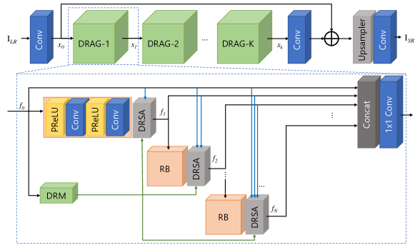
Figure 1: The framework of the proposed dynamic residual self-attention network (DRSAN). The upper figure shows that it consists of convolution layers (Conv), an upsampling network (Upsampler), and our basic building block DRAGs (dynamic residual attention groups). The lower figure describes the DRAG, which consists of an RB (residual block), a DRSA (dynamic residual self-attention), a DRM (dynamic residual module), a concatenation (Concat), and a $1\times 1$ convolution, where the RB is structured as a cascade of Convs and PReLUs (parametric rectified linear units) [37]. The signal flow inside the DRAG, including the function of DRSA, is detailed in Fig. 2.

II Related Works

II-A CNNs for SISR

SRCNN [8] is the first work to apply CNN to the SR task, which outperforms previous works [9, 10, 11, 12] with a simple 3-layer CNN. Dong et al. simplified the problem by upsampling the input LR image with bicubic interpolation, turning the problem into refining an upsampled coarse LR image into an HR image. Within this pre-upsampling framework, VDSR [16] has shown an excellent performance by deepening the network with a residual learning scheme. However, the upsampling strategy causes artifacts, such as amplified noise and blurring. More importantly, the enlarged input image increases the feature size, which is computationally inefficient. ESPCN [38] introduced an efficient pixel-shuffle layer to reduce the computational inefficiency of previous methods by processing features in the LR space and upsampling it at the end of the network. This post-upsampling strategy has occupied the mainstream of SR research, combined with residual learning. As residual learning [13] eases training and since post-upsampling improves the computational efficiency, deeper and deeper SISR networks with excellent performances have been proposed [17, 39, 18]. There have also been some methods to propose new architectures and objectives suitable for preserving the structures while super-resolving the images [40] or for deploying multi-receptive fields with fast computation [41]. For more detailed insights into CNN architectures and objectives for SISR, refer to the review in [42].

II-B Lightweight SISR

Deepening the network guarantees an excellent performance boost at the cost of heavy parameters and computational resources [17, 39, 43, 18]. Some of the recent models’ computational costs exceed certain extents, proving that it is difficult to apply them to real-time scenarios. Hence, various lightweight SR networks have also been proposed for practical applications. For example, DRCN [19], DRRN [20], and DRFN [44] exploited recursive structures to reduce the number of parameters. CARN [21] also showed an acceptable performance with a few parameters using a recursive cascading mechanism. FALSR [22] automated the lightweight SR model design based on neural architecture search (NAS) approach [45]. AWSRN [23] and A²FNet [24] applied adaptive weights to residual paths, achieving a good balance between the reconstruction performance and the computational cost. While lightweight networks are efficient and effective, most of them are designed manually, requiring much trial and error to achieve an optimal performance. Additionally, these networks have predefined fixed structures, and thus, process all of the images with the same operation, which may not be optimal for accurate SR image reconstruction with limited network capacity. For instance, some features might be informative for a certain input LR image, though it may be redundant for others. In comparison, our method learns the correlation between input image statistics and residual paths during training, and then changes its residual connections depending on the input image. Hence, our method can represent various features as a linear combination of features from preceding blocks.

II-C Attention Mechanisms for SISR

The attention mechanism inspired by neuroscience [46], has brought substantial improvements to neural network applications. By adjusting the weights, the attention mechanism assigns priorities to important features. SENet [34] proposed a CA scheme, which has been widely adopted in SR networks due to its simplicity, effectiveness, and small computational overheads. The CA gives a 1D (1$\times$1$\times$C) attention map for scaling the features by channel-wise importance. Roy et al. [47] proposed spatial attention (SA), obtained from spatial-wise squeeze and excitation. The SA yields a 2D (H$\times$W$\times$1) attention map and prioritizes notable areas. A-CubeNet [27], LAMRN [33], GLADSR [48], and MAMSR [49] jointly utilize SA and CA, showing that using multiple attention methods can improve the reconstruction performance. SAN [50] proposed another attention mechanism and considered second-order feature statistics for accurate SR reconstruction. Recently, inspired by SCNet [51], Zhao et al. [28] proposed a pixel attention (PA) scheme for a lightweight network. The network computes a 3D attention map with a small computational cost, showing that this type of map is effective for accurate SR reconstruction. While these previous works have shown excellent performances, they have only focused on the features from the residual blocks and did not consider the features from the skip connections. In addition, the existing methods have been gradually improved by using increasingly complex attention methods, which require additional attention modules and higher computational costs. Compared to previous methods, we apply the attention scheme to skip connections, named DRA, which allows the network to utilize various combinations of features from preceding layers to cope with the varying input statistics. This dynamic structure gives the network flexibility against diverse image statistics, boosting the network’s representational power with a limited capacity. Additionally, we propose RSA, which generates a 3D attention map with the features from the residual block. By cooperating with a residual structure, RSA can generate attention coefficients without additional modules or complex computation.

III Proposed Method

III-A Network Structure

As shown in Fig. 1, the proposed DRSAN consists of three modules: a feature extraction module (Conv), a non-linear mapping module with multiple dynamic residual attention groups (DRAGs), and a reconstruction module (Upsampler and Conv).

III-A1 Feature Extraction Module

The feature extraction module is the first convolutional layer with a kernel size of 3. The input LR image is fed to the first convolutional layer, which can be formulated as follows:

$$x_{0}=\text{F}_{ext}(\text{I}_{LR}),$$ (1)

where $\text{F}_{ext}$ denotes the feature extraction operation and $\text{I}_{LR}$ denotes the LR input image. The first convolutional layer performs shallow feature extraction, and the output feature $x_{0}$ is sent to the non-linear mapping module and the reconstruction module.

III-A2 Nonlinear Mapping Module

The nonlinear mapping module consists of multiple DRAGs, which extract information to reconstruct an HR image. The shallow feature $x_{0}$ is processed with stacked DRAGs as follows:

$$x_{k}=\text{F}_{DRAG}^{k}(x_{k-1}),\;k=1,2,...,K,$$ (2)

where $\text{F}_{DRAG}^{k}$ denotes the DRAG operation of the $k$-th DRAG, and $K$ denotes the number of DRAGs in the DRSAN. The proposed DRAG consists of multiple residual blocks (RBs), dynamic residual module (DRM), and dynamic residual self-attention (DRSA) modules, as illustrated in the lower part of Fig. 1. Additionally, the signal flow in a part of the DRAG is described in Fig. 2. The figure shows that the DRM controls residual connections to adaptively combine the features, allowing the DRAG to combine the features of residual blocks with appropriate weights to deal with various input image properties. The figure also illustrates that DRSA exploits two attention mechanisms: DRA (upper part of the gray box) and RSA (lower part). The details of the DRAG and its attention mechanism are described in the next subsection (Sec. III.B).

III-A3 Reconstruction Module

Extracted deep feature $x_{K}$ is then upscaled through the upsampler network, which is described as

$$x_{up}=\text{G}_{up}(\text{F}_{3\times 3}(x_{K})+x_{0}),$$ (3)

where $\text{G}_{up}$ denotes the upsampling function, which consists of one convolutional layer and the pixel-shuffle layer [38]. Following the global residual learning scheme [16], shallow feature $x_{0}$ is added to deep feature $x_{K}$ before the pixel-shuffle operation. The pixel-shuffle layer transforms the shape of the input feature with the depth-to-space operation. After upscaling, the network reconstructs the super-resolved (SR) image as follows:

$$\text{I}_{SR}=\text{F}_{rec}(x_{up}),$$ (4)

where $\text{I}_{SR}$ is the reconstructed SR image, and $\text{F}_{rec}$ is the operation of the last convolutional layer with a kernel size of 3.

III-B Dynamic Residual Attention Group (DRAG)

As a building block of the nonlinear mapping module, the DRAG extracts residual features to reconstruct an accurate HR image. It has three main elements: residual blocks, DRMs, and DRSAs.

III-B1 Dynamic Residual Module (DRM)

Fig.2 illustrates the signal flow around and inside the $n$-th RB and DRSA, along with the DRM. The DRM is a simple module with two convolutional layers, which controls residual connections between the residual blocks in a DRAG. Notably, the DRM does not use the sigmoid function as an activation function to exploit residual coefficients in wide ranges for feature diversity. It decides how to combine the residual features, i.e.,, computes DRA parameters ($r_{k}^{n}$ shown above the DRSA in Fig. 2), considering the given input feature of a DRAG. Formally, the DRM determines the DRA parameters as follows:

$$\begin{split}r&=\text{M}_{DRM}(f_{0})\\ &=\text{P}_{avg}(\text{F}_{out}(\text{PReLU}(\text{F}_{in}(f_{0}))))\\ &=[r_{0}^{1},r_{0}^{2},r_{1}^{2},r_{0}^{3},r_{1}^{3},r_{2}^{3},\cdots,r_{0}^{N},r_{1}^{N},\cdots,r_{N-1}^{N}],\end{split}$$ (5)

where $\text{M}_{DRM}$ denotes DRM operation, $\text{P}_{avg}$ denotes global average pooling, $\text{F}_{in}$ and $\text{F}_{out}$ denote convolutional layers, $f_{0}$ denotes the input feature of DRAG, and $N$ denotes the number of residual blocks in a DRAG. During the training process, DRM learns the correlation between input image statistics and residual paths, which helps the network exploit proper features among the low- and high-level features with various combinations.

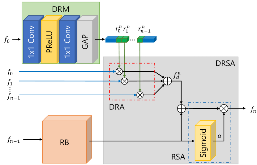
Figure 2: The signal flow graph inside the DRAG, and the function of the $n$-th DRSA. The DRSA outputs the $n$-th residual feature ($f^{n}$) as a combination of $f_{d}^{n}$ (addition of previous features with DRA) and $\alpha$ (RSA formed by the RB and sigmoid). The DRM determines the DRA that reflects the input properties.

III-B2 Dynamic Residual Self-Attention (DRSA)

The proposed DRSA is an attention scheme that allows the network to exploit various combinations of residual features in DRAGs. As shown in Fig. 2 and Eq. (5), DRM determines the DRA parameters $r$ considering the input feature statistics. These parameters scale the corresponding residual paths in DRAG, allowing the network to adaptively change its residual structure for the input image. The residual feature $f_{n}$ of the $n$-th residual block can be described as

$$f_{n}=(\text{F}_{res}^{n}(f_{n-1})+f_{d}^{n})\cdot\alpha,$$ (6)

where $\text{F}_{res}^{n}$ denotes convolution operation of the $n$-th residual block, $f_{d}^{n}$ denotes dynamic residual feature for the $n$-th residual block, and $\alpha$ denotes the residual self attention coefficient. With the DRA attention parameter $r^{n}=[r_{0}^{n},...,r_{n-1}^{n}]$ decided by the DRM, dynamic reisdual feature $f_{d}^{n}$ can be formulated as

$$f_{d}^{n}=(r_{0}^{n}\cdot f_{0}+r_{1}^{n}\cdot f_{1}+...+r_{n-1}^{n}\cdot f_{n-1}).$$ (7)

This indicates that all features from preceding residual blocks of a DRAG are potentially connected, allowing DRAG to utilize diverse combinations of residual features. After the dynamic residual feature $f_{d}^{n}$ is computed, the residual self-attention is applied. The residual self-attention coefficient $\alpha$ is calculated as

$$\alpha=\sigma(\text{F}_{res}^{n}(f_{n-1})),$$ (8)

where $\sigma$ denotes sigmoid activation function. This simple yet efficient attention scheme yields a 3D attention map, which scales features channel-wisely and spatial-wisely. The proposed RSA recalibrates the network features and helps the network focus on more informative features.

After all of the residual features ${f_{1},f_{2},...,f_{N}}$ are decided, the output of the $k$-th DRAG $x_{k}$ can be formulated as follows:

$$x_{k}=\text{F}_{1\times 1}(\text{concat}[f_{0},f_{1},...,f_{N}]),$$ (9)

where $\text{F}_{1\times 1}$ denotes the 1$\times$1 convolution, and $concat$ denotes the channel-wise concatenation of features.

TABLE I: Implementation details of the proposed method. $N$ means the number of residual blocks in a DRAG, $k$ stands for the $k$-th DRAG, $c$ is the number of channels in a convolutional layer, $s$ is the scaling factor, and GAP indicates the global average pooling.

Function		Layer	Kernel	Channels (Input, Output)
$\text{F}_{ext}$		Conv	$3\times 3$	(3, $c$)
$\text{F}^{k}_{DRAG}$	$\text{F}_{res}$	PReLU	-	-
		Conv	$3\times 3$	($c$, $c$)
		PReLU	-	-
		Conv	$3\times 3$	($c$, $c$)
	$\text{M}_{DRM}$	Conv	$1\times 1$	($c$, 16)
		PReLU	-	-
		Conv	$1\times 1$	(16, $\frac{N\cdot(N+1)}{2}$)
		GAP	-	-
	$\text{F}_{1\times 1}$	Conv	$1\times 1$	($c$$\cdot$N, $c$)
$\text{F}_{3\times 3}$		Conv	$3\times 3$	($c$, $c$)
$\text{G}_{up}$	$\times 2,\times 3$	Conv	$3\times 3$	($c$, $c$$\cdot s^{2}$)
		PixelShuffle	-	-
	$\times 4$	Conv	$3\times 3$	($c$, $c$$\cdot 2^{2}$)
		PixelShuffle	-	-
		Conv	$3\times 3$	($c$, $c$$\cdot 2^{2}$)
		PixelShuffle	-	-
$\text{F}_{rec}$		Conv	$3\times 3$	($c$, 3)

IV Experimental Results

IV-A Dataset

The DRSAN is trained with DIV2K dataset [52], which consists of 800 high-resolution training images. We use RGB patches with a size of 48$\times$48 for training. Additionally, we perform data augmentation on the training dataset with flips and rotations. We evaluate the peak signal-to-noise ratio (PSNR) and structural similarity index (SSIM) [53] on the Y channel of the test images, using four SR benchmark datasets: Set5 [54], Set14 [55], B100 [56], and Urban100 [57].

IV-B Training Details

The mini-batch size is set to 16. We use ADAM optimizer for network training with $\beta_{1}=0.9$, $\beta_{2}=0.999$, and $\epsilon=10^{-8}$. The learning rate is initialized as $2\times 10^{-4}$, and decayed with the factor of 0.85 for every $2\times 10^{5}$ iterations. The L1 is used as a loss function for training.

IV-C Implementation Details

To explore the trade-off between depth and channel on our model, we prepare five variants of DRSAN: DRSAN-32s, DRSAN-32m, DRSAN-32l, DRSAN-48s, and DRSAN-48m, which have different numbers of channels and layers. Small-scale models are suffixed by “-s,” medium-scale by “-m,” and large-scale by “-l,” and each model has 4, 8, and 10 DRAGs, respectively. The models using 32 channels for convolutional layers are suffixed by “-32,” and the models using 48 channels by “-48.” To generate networks with similar complexities to the compared methods, we make the DRAGs have three residual blocks ($N=3$) for DRSAN-48 models and four residual blocks ($N=4$) for DRSAN-32 models. The DRM in DRAGs has 16 filters for the first convolutional layer. The second convolutional layer in DRM has 6 filters for 48 channel models and 10 filters for 32 channel models, where 6 and 10 correspond to $\frac{N\cdot(N+1)}{2}$ for $N=3$ and 4, respectively.

As the upsampler module, we use the ESPCN method [38]. The last convolutional layer in the reconstruction module has three channels to reconstruct an RGB image. More details about the model structure are described in Table I. All results are evaluated on the NVIDIA TITAN XP GPU device.

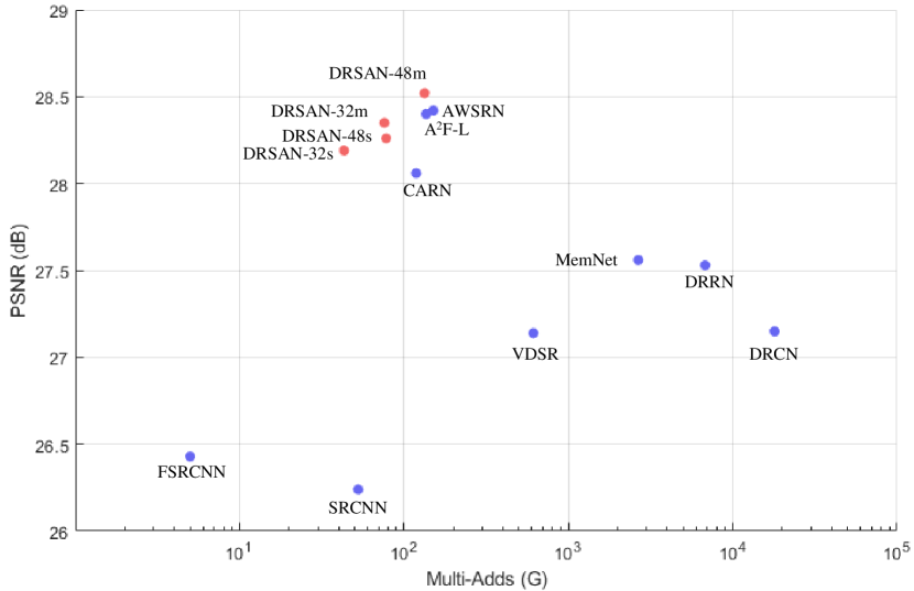
Figure 3: Performance comparison between the SOTA lightweight networks and our methods. The results are evaluated on the Urban100 ($\times 3$) dataset.

TABLE II: Quantitative comparisons of our models with the previous SOTA lightweight networks on benchmark datasets. Our models are marked in bold. The best performance is denoted in red, and the second-best performance is denoted in blue. “Param” is the number of parameters, and “Multi-Adds” is the number of multiply-accumulate operations.

Scale	Scope	Model	Param	Multi-Adds	Set5	Set14	B100	Urban100
					PSNR / SSIM	PSNR / SSIM	PSNR / SSIM	PSNR / SSIM
$\times 2$	$<$ 500 K	FSRCNN	0.01 M	6.0G	37.00 / 0.9558	32.63 / 0.9088	31.53 / 0.8920	29.88 / 0.9020
		DRRN	0.30 M	6796.9G	37.74 / 0.9591	33.23 / 0.9136	32.05 / 0.8973	31.23 / 0.9188
		A2F-SD	0.31 M	71.2G	37.91 / 0.9602	33.45 / 0.9164	31.79 / 0.8986	31.79 / 0.9246
		A2F-S	0.32 M	71.7G	37.79 / 0.9597	33.32 / 0.9152	31.99 / 0.8972	31.44 / 0.9211
		FALSR-B	0.33 M	74.7G	37.61 / 0.9585	33.29 / 0.9143	31.97 / 0.8967	31.28 / 0.9191
		AWSRN-SD	0.35 M	79.6G	37.86 / 0.9600	33.41 / 0.9161	32.07 / 0.8984	31.67 / 0.9237
		AWSRN-S	0.40 M	91.2G	37.75 / 0.9596	33.31 / 0.9151	32.00 / 0.8974	31.39 / 0.9207
		FALSR-C	0.41 M	93.7G	37.66 / 0.9586	33.26 / 0.9140	31.96 / 0.8965	31.24 / 0.9187
		DRSAN-32s (Ours)	0.37 M	85.5G	37.99 / 0.9606	33.57 / 0.9177	32.16 / 0.8999	32.10 / 0.9279
	$<$ 1000 K	IDN	0.55 M	-	37.83 / 0.9600	33.30 / 0.9148	32.08 / 0.8985	31.27 / 0.9196
		VDSR	0.66 M	612.6G	37.53 / 0.9587	33.03 / 0.9124	31.90 / 0.8960	30.76 / 0.9140
		MemNet	0.68 M	2662.4G	37.78 / 0.9597	33.28 / 0.9143	32.08 / 0.8978	31.31 / 0.9195
		IMDN	0.69 M	-	38.00 / 0.9605	33.63 / 0.9177	32.19 / 0.8996	32.17 / 0.9283
		LapSRN	0.81 M	29.9G	37.52 / 0.9590	33.08 / 0.9130	31.80 / 0.8950	30.41 / 0.9100
		SelNet	0.97 M	225.7G	37.89 / 0.9598	33.61 / 0.9160	32.08 / 0.8984	-
		A2F-M	1.00 M	224.2G	38.04 / 0.9607	33.67 / 0.9184	32.18 / 0.8996	32.27 / 0.9294
		DRSAN-48s (Ours)	0.65 M	150.0G	38.08 / 0.9609	33.62 / 0.9175	32.19 / 0.9002	32.16 / 0.9286
		DRSAN-32m (Ours)	0.69 M	159.3G	38.11 / 0.9609	33.64 / 0.9185	32.21 / 0.9005	32.35 / 0.9304
		DRSAN-32l (Ours)	0.85 M	196.3G	38.13 / 0.9610	33.72 / 0.9189	32.24 / 0.9009	32.41 / 0.9312
	$<$ 2000 K	FALSR-A	1.02 M	234.7G	37.82 / 0.9595	33.55 / 0.9168	31.12 / 0.8987	31.93 / 0.9256
		AWSRN-M	1.06 M	244.1G	38.04 / 0.9605	33.66 / 0.9181	32.21 / 0.9000	32.23 / 0.9294
		A2F-L	1.36 M	306.1G	38.09 / 0.9607	33.78 / 0.9192	32.23 / 0.9002	32.46 / 0.9313
		OISR-RK2-s	1.37 M	316.2G	37.98 / 0.9604	33.58 / 0.9172	32.18 / 0.8996	32.09 / 0.9281
		AWSRN	1.40 M	320.5G	38.11 / 0.9608	33.78 / 0.9189	32.26 / 0.9006	32.49 / 0.9316
		CARN	1.59 M	222.8G	37.76 / 0.9590	33.52 / 0.9166	32.09 / 0.8978	31.92 / 0.9256
		DRCN	1.77 M	17974G	37.63 / 0.9588	33.04 / 0.9118	31.85 / 0.8942	30.75 / 0.9133
		DRSAN-48m (Ours)	1.19 M	274.6G	38.14 / 0.9611	33.75 / 0.9188	32.25 / 0.9010	32.46 / 0.9317
$\times 3$	$<$ 500 K	FSRCNN	0.01 M	5.0G	33.16 / 0.9140	29.43 / 0.8242	28.53 / 0.7910	26.43 / 0.8080
		DRRN	0.30 M	6797G	34.03 / 0.9244	29.96 / 0.8349	28.95 / 0.8004	27.53 / 0.8378
		A2F-SD	0.32 M	31.9G	34.23 / 0.9259	30.22 / 0.8395	29.01 / 0.8028	27.91 / 0.8465
		A2F-S	0.32 M	32.3G	34.06 / 0.9241	30.08 / 0.8370	28.92 / 0.8006	27.57 / 0.8392
		AWSRN-SD	0.39 M	39.5G	34.18 / 0.9273	30.21 / 0.8398	28.99 / 0.8027	27.80 / 0.8444
		AWSRN-S	0.48 M	48.6G	34.02 / 0.9240	30.09 / 0.8376	28.92 / 0.8009	27.57 / 0.8391
		DRSAN-32s	0.41 M	43.2G	34.41 / 0.9272	30.27 / 0.8413	29.08 / 0.8056	28.19 / 0.8529
	$<$ 1000 K	IDN	0.55 M	-	34.11 / 0.9253	29.99 / 0.8354	28.95 / 0.8013	27.42 / 0.8359
		VDSR	0.66 M	612.6G	33.66 / 0.9213	29.77 / 0.8314	28.82 / 0.7976	27.14 / 0.8279
		MemNet	0.68 M	2662.4G	34.09 / 0.9248	30.00 / 0.8385	28.96 / 0.8001	27.56 / 0.8376
		IMDN	0.70 M	-	34.36 / 0.9270	30.32 / 0.8417	29.09 / 0.8046	28.17 / 0.8519
		DRSAN-32m (Ours)	0.74 M	76.0G	34.50 / 0.9278	30.39 / 0.8437	29.13 / 0.8065	28.35 / 0.8566
		DRSAN-48s (Ours)	0.75 M	78.0G	34.47 / 0.9274	30.35 / 0.8422	29.11 / 0.8060	28.26 / 0.8542
	$<$ 2000 K	A2F-M	1.00 M	100.0G	34.50 / 0.9278	30.39 / 0.8427	29.11 / 0.8054	28.28 / 0.8546
		AWSRN-M	1.14 M	116.6G	34.42 / 0.9275	30.32 / 0.8419	29.13 / 0.8059	28.26 / 0.8545
		SelNet	1.16 M	120G	34.27 / 0.9257	30.30 / 0.8399	28.97 / 0.8025	-
		A2F-L	1.37 M	136.3G	34.54 / 0.9283	30.41 / 0.8436	29.14 / 0.8062	28.40 / 0.8574
		AWSRN	1.48 M	150.6G	34.52 / 0.9281	30.38 / 0.8426	29.16 / 0.8069	28.42 / 0.8580
		CARN	1.59 M	118.8G	34.29 / 0.9255	30.29 / 0.8407	29.06 / 0.8034	28.06 / 0.8493
		DRCN	1.77 M	17974G	33.82 / 0.9226	29.76 / 0.8311	28.80 / 0.7963	27.15 / 0.8276
		DRSAN-48m (Ours)	1.29 M	133.4G	34.59 / 0.9286	30.42 / 0.8443	29.18 / 0.8079	28.52 / 0.8593
$\times 4$	$<$ 500 K	FSRCNN	0.01 M	4.6G	30.48 / 0.8628	27.49 / 0.7503	26.90 / 0.7101	24.52 / 0.7221
		DRRN	0.30 M	6797G	31.68 / 0.8888	28.21 / 0.7720	27.38 / 0.7284	25.44 / 0.7638
		AWSRN-SD	0.44 M	25.4G	31.98 / 0.8921	28.46 / 0.7786	27.48 / 0.7368	25.74 / 0.7746
		DRSAN-32s (Ours)	0.41 M	30.5G	32.15 / 0.8935	28.54 / 0.7813	27.54 / 0.7364	26.06 / 0.7858
	$<$ 1000 K	IDN	0.55 M	-	31.82 / 0.8903	28.25 / 0.7730	27.41 / 0.7297	25.41 / 0.7632
		AWSRN-S	0.59 M	37.7G	31.77 / 0.8893	28.35 / 0.7761	27.41 / 0.7304	25.56 / 0.7678
		VDSR	0.66 M	612.6G	31.35 / 0.8838	28.01 / 0.7674	27.29 / 0.7251	25.18 / 0.7524
		MemNet	0.68 M	2662.4G	31.74 / 0.8893	28.26 / 0.7723	27.40 / 0.7281	25.50 / 0.7630
		IMDN	0.72 M	-	32.21 / 0.8948	28.58 / 0.7811	27.56 / 0.7353	26.04 / 0.7838
		LapSRN	0.81 M	149.4G	31.54 / 0.8850	28.19 / 0.7720	27.32 / 0.7280	25.21 / 0.7560
		DRSAN-32m (Ours)	0.73 M	49.0G	32.30 / 0.8954	28.66 / 0.7838	27.61 / 0.7381	26.26 / 0.7920
		DRSAN-48s (Ours)	0.73 M	57.6G	32.25 / 0.8945	28.55 / 0.7817	27.59 / 0.7374	26.14 / 0.7875
	$<$ 2000 K	A2F-M	1.01 M	56.7G	32.28 / 0.8955	28.62 / 0.7828	27.58 / 0.7364	26.17 / 0.7892
		AWSRN-M	1.25 M	72G	32.21 / 0.8954	28.65 / 0.7832	27.60 / 0.7368	26.15 / 0.7884
		A2F-L	1.37 M	77.2G	32.32 / 0.8964	28.67 / 0.7839	27.62 / 0.7379	26.32 / 0.7931
		SelNet	1.42 M	83.1G	32.00 / 0.8931	28.49 / 0.7783	27.44 / 0.7325	-
		AWSRN	1.59 M	91.1G	32.27 / 0.8960	28.69 / 0.7843	27.64 / 0.7385	26.29 / 0.7930
		CARN	1.59 M	90.9G	32.13 / 0.8937	28.60 / 0.7806	27.58 / 0.7349	26.07 / 0.7837
		DRCN	1.77 M	17974G	31.53 / 0.8854	28.02 / 0.7670	27.23 / 0.7233	25.14 / 0.7510
		DRSAN-48m (Ours)	1.27 M	88.7G	32.34 / 0.8960	28.65 / 0.7841	27.63 / 0.7390	26.33 / 0.7936

TABLE III: Quantitative comparisons of our model with the SOTA SR methods on benchmark datasets ($\times$4).

Model	Param	Set5	Set14	BSDS100	Urban100
EDSR	43.1 M	32.46 dB	28.80 dB	27.71 dB	26.64 dB
RDN	22.3 M	32.47 dB	28.81 dB	27.72 dB	26.61 dB
RCAN	15.6 M	32.63 dB	28.87 dB	27.77 dB	26.82 dB
SAN	15.9 M	32.64 dB	28.92 dB	27.78 dB	26.79 dB
DRN	9.8 M	32.74 dB	28.98 dB	27.83 dB	27.03 dB
DRSAN	0.7 M	32.30 dB	28.66 dB	27.61 dB	26.26 dB

TABLE IV: Comparison of parameter, memory usage, inference time and performance between SR methods. Memory represents GPU memory used by total tensor of each model. Inference time is calculated on B100 ($\times$4) dataset

.

Model	Param	Memory	Running time	PSNR
CARN-M	0.41 M	3.0MB	10.473ms	27.44 dB
VDSR	0.66 M	3.7MB	22.618ms	27.29 dB
A2F-L	1.37 M	11.7MB	16.524ms	27.62 dB
DRN-S	4.8 M	20.7MB	41.519ms	27.78 dB
RCAN	15.6 M	61.3MB	75.448ms	27.76 dB
DRSAN-32s	0.41 M	3.4MB	8.291ms	27.54 dB
DRSAN-48m	1.27 M	6.7MB	13.317ms	27.63 dB

IV-D Model Analysis

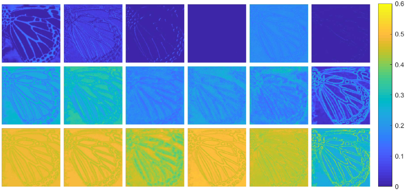
Figure 4: Activation maps of the SA (the first row), PA (second), and DRSA (third) from the residual blocks of the networks. For visualization, the results of PA and DRSA are obtained by averaging channel-wise attention maps.

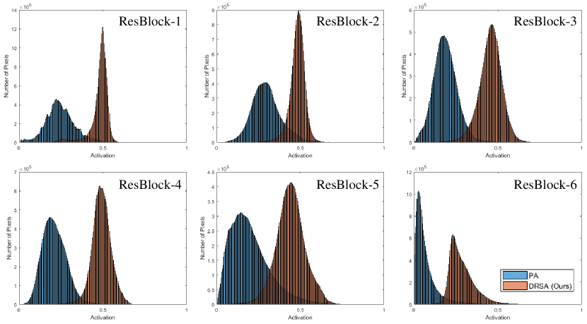
Figure 5: Histogram of activation values of PA and DRSA. Each histogram represents the frequency distribution of the activation values from each block of the network. Activation values are collected from images of the Set5 ($\times 2$) dataset.

In this section, we perform additional experiments to understand how DRSA behaves in the network and its differences compared with previous works.

IV-D1 Activation Analysis

First, we compare the activation maps with the networks using SA, PA, and DRSA. The activation maps are shown in Fig. 4, obtained by averaging attention maps in a channel. Unlike PA and DRSA, SA produces a 2D attention map (H$\times$W$\times$1) and applies the same attention weights to all channels of the feature. Each channel in the feature maps may require different attention maps for the optimal solution, and this lack of flexibility leads to almost inactivated attention maps, such as the first row’s 4th and 6th attention maps of SA, implying that the 2D attention scheme is less helpful for some residual blocks.

However, as shown in the 2nd and 3rd columns of Fig. 4, the attention schemes yielding 3D attention maps (H$\times$W$\times$C) are always active in any residual blocks, implying that each channel in the residual feature may require different attention weights for the optimal results. Additionally, note that there is some shared tendency between PA and DRSA in attention weight decision policy. We observe that both attention methods attempt to assign higher weights to the texture part, except for the last residual block. In contrast, the edge part has higher attention weights in the last residual block located immediately before the upsampler network. This result indicates that both attention schemes work differently depending on the location, especially at the network’s last residual block.

Next, we compare the histogram of activation maps with two different attention models to explore the influence of the proposed DRSA. Each histogram in Fig. 5 represents the activation map at each network’s residual block. The histograms in Fig. 5 are obtained by using Set5 ($\times 2$) images as the input. As shown in Fig. 5, PA has values that range near zero, making the network suppress the residual block’s feature values. On the other hand, the DRSA has values that range near 0.5, enabling the network to scale the features with higher values than those of the PA. In other words, our DRSA tends to boost more attentive features and suppress less informative features.

Therefore, the PA mostly turns off the unimportant feature values for the last residual block, when struggling with the limited range near 0. In contrast, our DRSA rescales the feature values with more discriminative importance, assigning different attention values even with the less important features.

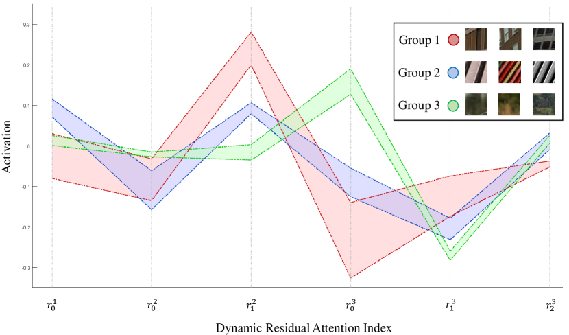
Figure 6: The activation values of DRA in the 1st DRAG using different patches as input. Patches with similar DRA values are grouped. Patches are collected from images of benchmark datasets ($\times$2).

IV-D2 Behavior Analysis

As stated previously, we devised DRA to have different values by the DRM, depending on input image properties. To investigate this, we group input patches with similar properties and compare their DRA value distributions in Fig. 6. We use DRA values of the first DRAG of the ablation model used in the ablation study for this visualization. We can see that the variations of DRA values have different forms depending on image groups. Specifically, the images in Group 1 have rectangular textures, Group 2 has strong edges, Group 3 has almost no edges or textures, and DRA values have different behavior depending on the group. Notably, we observe that the variation of DRA values of Group 3, which lacks edges and high-frequency information, is relatively small. On the other hand, the DRA values dynamically change depending on the shapes of edges and textures. We may interpret that the edge and high-frequency textures are discriminative features for our DRA, as their values change dynamically to find effective features for reconstructing the final result.

To examine whether the DRA values affect the SR reconstruction, we reconstruct specific images using DRAs extracted from different images with different characteristics, as shown in Fig. 7. The first ”SR” column shows the images to be super-resolved, and ”DRA$n$” columns are the super-resolved images when the DRA values are given by each of the image patches shown in the first row. Specifically, DRA1 is the case in which DRA values are given by the smooth patch, DRA2 by the strong horizontal edges, and DRA3 by diagonal edges. Additionally, the blue figure columns on the right side of DRA$n$ columns are the differences from the corresponding original SR results. The figure shows that the changes in DRA lead to changes in the SR results of the network. For example, the 4th and last rows show that the stripe patterns are best reconstructed by the DRA learned from similar patches, as the differences are small for this case (last column). Additionally, most of the changes are observed near edges in images, suggesting that DRA is mainly involved in reconstructing the edge portion of the image. In summary, the results imply that DRA helps SR reconstruction by focusing on edge-related features. We hope that our study may provide a small clue to understanding the features of SR networks for future research.

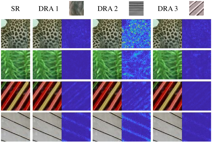
Figure 7: The reconstructed images using DRA from different patches and their visualized difference maps. The difference map is calculated on the Y channel of the image and its original SR image. Patches are collected from images of benchmark datasets ($\times$2).

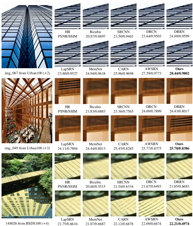
Figure 8: Qualitative comparisons with the bicubic degradation model on the BSDS100 and Urban100 datasets. The best results are marked in bold.

IV-E Comparison with state-of-the-art methods

In this section, we compare the proposed DRSAN with several lightweight SR networks and networks with parameters similar to lightweight methods, including FSRCNN [58], VDSR [16], DRCN [19], DRRN [20], MemNet [25], SelNet [59], IDN [60], IMDN [61], LapSRN [62], CARN [21], FALSR [22], OISR [63], AWSRN [23], and A²FNet [24]. Additionally, we compare our method with the heavyweight SOTA SR methods requiring more than $2\,$M parameters, including EDSR [17], RDN [43], RCAN [39], SAN [50], and DRN [64]. For comparing the complexities of the networks, we compare the number of parameters and the number of operations by Multi-Adds, which is the number of multiply-accumulate operations for a single 720p (1280$\times$720) HR image. For detailed comparisons between SR methods with various network capacities, we split the comparison results into several groups, according to the upscaling factor and the number of parameters.

Table II shows the comparison of complexity and performance between lightweight SR models. Our models perform better than existing methods in the same parameter scope, indicating an efficient trade-off between reconstruction performance and complexity. Note that our DRSAN-32m model shows comparable performance to the AWSRN-M and A²F-M models, which have more parameters and operations than ours. Additionally, we observe that DRSAN-32 models outperform DRSAN-48 models with similar network capacities. It suggests increasing the depth, rather than the channels, to obtain a better performance with similar network complexity.

Table III compares the complexity and performance between the heavyweight SOTA SR methods and our DRSAN-32m. It can be seen that our model requires at least ten times fewer parameters than the heavy models while delivering competitive results. Precisely, our lightweight network shows a similar performance ($0.1\sim 0.2\,$dB) as heavy networks in the case of the BSD100 dataset, and the difference becomes larger ($0.4\sim 0.8\,$dB) in the case of the Urban100 dataset, which consists of images having complex structures.

In Table IV, we compare the inference time and memory usage between the SOTA methods and ours. Compared with lightweight models with similar parameters, our methods show remarkable performances while requiring less inference time. Compared with heavy SR methods, our methods require three to nine times less memory and inference time while sacrificing $0.1$ to $0.2\,$dB of performance. These observations suggest that our method has an efficient trade-off between model complexity and performance.

Finally, we show qualitative comparisons on the BSDS100 and Urban100 datasets in Fig. 8. We can see that other methods struggle with blurring and aliasing artifacts at the challenging stripe patterns. In contrast, our method reconstructs more details and reduces the blurring artifacts. These results indicate that our dynamic residual network scheme shows a comparable performance to handcrafted networks by using the proper combination of residual features considering the input image characteristics.

IV-F Ablation Study

TABLE V: Ablation study on the proposed DRSA. Res is the original residual connection from SRResNet, and All Res indicates all possible residual connections in DRAG.

Res	All Res	DRAG			Params	PSNR
		DRA	RSA	Concat
$\checkmark$					357 K	31.54 dB
$\checkmark$			$\checkmark$		357 K	31.66 dB
$\checkmark$			$\checkmark$	$\checkmark$	375 K	31.73 dB
		$\checkmark$	$\checkmark$		358 K	31.71 dB
	$\checkmark$		$\checkmark$	$\checkmark$	375 K	31.68 dB
		$\checkmark$		$\checkmark$	377 K	31.70 dB
		$\checkmark$	$\checkmark$	$\checkmark$	377 K	31.82 dB

TABLE VI: Comparison of the network performance between sigmoid and hyperbolic tangent (Tanh) as an activation function of DRM.

Activation	Sigmoid	Tanh	None
PSNR	$31.77\,$dB	31.79 dB	31.82 dB

TABLE VII: Comparison of channel attention (CA), spatial attention (SA), pixel attention (PA), and the proposed DRSA. The results show average PSNR evaluated on the Set5, Set14, BSDS100, and Urban100.

Model	Baseline	CA	SA	PA	DRSA (Ours)
Params	375 K	378 K	376 K	389 K	377 K
PSNR	32.06 dB	32.13 dB	32.10 dB	32.16 dB	32.18 dB

IV-F1 Dynamic Residual Connection

We first demonstrate the effectiveness of the DRAG structure by replacing its components with well-known methods. To examine the influence of the DRA, we replace it with a residual connection from SRResNet [65] and all possible residual connections, which amounts to DRA without the parameters $r$. Additionally, we examine the effect of the RSA by applying it to two different residual connection methods: residual connection from SRResNet and our dynamic residual connection. As a baseline network, we use the DRSAN structure with 2 DRAGs trained with the DIV2K dataset.

Table V shows the performance of ablation models for Urban100 ($\times 2$) with different configurations. The first and second rows show that the RSA mechanism boosts $0.12\,$dB without any parameter increase. This tendency can also be seen in the 6th and 7th rows, which supports that the proposed RSA improves the network performance by jointly working with residual connections. The 3rd, 5th, and 7th rows indicate that simply connecting all preceding residual features does not improve the performance and sometimes even deteriorates its performance. These results show that the DRM properly recalibrates the weights of residual features.

Through extensive experiments, it was found that obviating the sigmoid activation function gives a better performance than using the sigmoid activation function in our case. However, the sigmoid generally helps stable convergence and obtains a better performance in most cases. We conjecture that the sigmoid can hamper the diversity of feature combinations necessary for our scheme because the sigmoid limits the range of output features between 0 and 1. The OISR, which is an SR network inspired by the ordinary differential equation [63], also scales the residual features to a value of 2 or $-1$, suggesting that it is more advantageous not to limit the range of scaling values. Table VI compares the performance of ablation models with different activation functions to see the change in performance depending on the activation function. As shown in Table VI, using hyperbolic tangent rather than sigmoid proves to perform slightly better. Furthermore, DRM without the activation function achieves better results than DRM with a hyperbolic tangent, indicating that limiting the range of scaling values degrades the network performance.

IV-F2 Residual Self-Attention

To examine the effectiveness of the proposed attention scheme, we conduct ablation experiments by replacing DRSA with popular attention schemes in SR, namely CA, SA, and PA. We use the same configurations in [35] for the CA and the SA. As a baseline, we use the DRSAN structure with two residual groups but without the DRSA.

The results are shown in Table VII, which compares the performance of attention schemes for Set5, Set14, BSDS100, and Urban100 ($\times 2$). As shown in Table VII, CA and SA improved the PSNR by $0.07\,$dB and $0.04\,$dB, respectively, with small increases of $1\,$K to $3\,$K in the number of parameters. Unlike 1D CA and 2D SA, PA [28] produces a 3D attention map with pointwise convolution (1$\times$1) for an accurate SR reconstruction. The PA brings a PSNR gain of $0.10\,$dB with a $13\,$K parameter increase. However, our DRSA shows a $0.12\,$dB performance boost with the rise of $2\,$K parameters, indicating that our attention scheme is competitive and efficient compared with previous works.

V Conclusion

We have proposed a dynamic residual network scheme for a lightweight SR system, utilizing diverse combinations of residual features considering the input statistics. Additionally, we have introduced RSA that boosts the network performance without additional modules by cooperating with the residual structure. The network design schemes and attention mechanisms are easily applicable for other residual networks without designing a complex network structure. Experimental results on well-known benchmark datasets have shown that our method achieves better or comparable performances to SOTA models with complex configurations. We will extend the dynamic residual network scheme to other restoration tasks as future work and release our code at https://github.com/saturnian77/DRSAN.

Karam Park received the BS degree in Electrical and Computer Engineering from Seoul National University, Seoul, Korea, in 2018. He is currently studying for a Ph.D. degree in Electrical and Computer Engineering from Seoul National University, Seoul, Korea. His main research interest is image processing based on deep learning.

Jae Woong Soh received the BS degree in Electrical and Computer Engineering from Seoul National University, Seoul, Korea, in 2016. He is currently studying for a Ph.D. degree in Electrical and Computer Engineering from Seoul National University, Seoul, Korea. His research interests include image processing, computer vision, and machine learning.

Nam Ik Cho received the BS, MS, and Ph.D. degrees in Control and Instrumentation Engineering from Seoul National University, Seoul, Korea, in 1986, 1988, and 1992. From 1991 to 1993, he was a research associate with the Engineering Research Center for Advanced Control and Instrumentation, Seoul National University. From 1994 to 1998, he was with the University of Seoul as an assistant professor of Electrical Engineering. In 1999, he joined the Department of Electrical and Computer Engineering, Seoul National University, where he is currently a professor. His research interests include image processing, adaptive filtering, digital filter design, and computer vision.

References

- [1] S. Peled and Y. Yeshurun, “Superresolution in mri: application to human white matter fiber tract visualization by diffusion tensor imaging,” Magnetic Resonance in Medicine: An Official Journal of the International Society for Magnetic Resonance in Medicine, vol. 45, no. 1, pp. 29–35, 2001.
- [2] W. Shi, J. Caballero, C. Ledig, X. Zhuang, W. Bai, K. Bhatia, A. M. S. M. de Marvao, T. Dawes, D. O’Regan, and D. Rueckert, “Cardiac image super-resolution with global correspondence using multi-atlas patchmatch,” in International conference on medical image computing and computer-assisted intervention. Springer, 2013, pp. 9–16.
- [3] M. W. Thornton, P. M. Atkinson, and D. Holland, “Sub-pixel mapping of rural land cover objects from fine spatial resolution satellite sensor imagery using super-resolution pixel-swapping,” International Journal of Remote Sensing, vol. 27, no. 3, pp. 473–491, 2006.
- [4] T. Goto, T. Fukuoka, F. Nagashima, S. Hirano, and M. Sakurai, “Super-resolution system for 4k-hdtv,” in 2014 22nd International Conference on Pattern Recognition. IEEE, 2014, pp. 4453–4458.
- [5] B. K. Gunturk, A. U. Batur, Y. Altunbasak, M. H. Hayes, and R. M. Mersereau, “Eigenface-domain super-resolution for face recognition,” IEEE transactions on image processing, vol. 12, no. 5, pp. 597–606, 2003.
- [6] L. Zhang, H. Zhang, H. Shen, and P. Li, “A super-resolution reconstruction algorithm for surveillance images,” Signal Processing, vol. 90, no. 3, pp. 848–859, 2010.
- [7] P. Rasti, T. Uiboupin, S. Escalera, and G. Anbarjafari, “Convolutional neural network super resolution for face recognition in surveillance monitoring,” in International conference on articulated motion and deformable objects. Springer, 2016, pp. 175–184.
- [8] C. Dong, C. C. Loy, K. He, and X. Tang, “Image super-resolution using deep convolutional networks,” IEEE transactions on pattern analysis and machine intelligence, vol. 38, no. 2, pp. 295–307, 2015.
- [9] J. Yang, J. Wright, T. S. Huang, and Y. Ma, “Image super-resolution via sparse representation,” IEEE transactions on image processing, vol. 19, no. 11, pp. 2861–2873, 2010.
- [10] H. Chang, D.-Y. Yeung, and Y. Xiong, “Super-resolution through neighbor embedding,” in Proceedings of the 2004 IEEE Computer Society Conference on Computer Vision and Pattern Recognition, 2004. CVPR 2004., vol. 1. IEEE, 2004, pp. I–I.
- [11] K. I. Kim and Y. Kwon, “Single-image super-resolution using sparse regression and natural image prior,” IEEE transactions on pattern analysis and machine intelligence, vol. 32, no. 6, pp. 1127–1133, 2010.
- [12] R. Timofte, V. De Smet, and L. Van Gool, “Anchored neighborhood regression for fast example-based super-resolution,” in Proceedings of the IEEE international conference on computer vision, 2013, pp. 1920–1927.
- [13] K. He, X. Zhang, S. Ren, and J. Sun, “Deep residual learning for image recognition,” in Proceedings of the IEEE conference on computer vision and pattern recognition, 2016, pp. 770–778.
- [14] C. Szegedy, S. Ioffe, V. Vanhoucke, and A. Alemi, “Inception-v4, inception-resnet and the impact of residual connections on learning,” in Proceedings of the AAAI Conference on Artificial Intelligence, vol. 31, no. 1, 2017.
- [15] F. Chollet, “Xception: Deep learning with depthwise separable convolutions,” in Proceedings of the IEEE conference on computer vision and pattern recognition, 2017, pp. 1251–1258.
- [16] J. Kim, J. K. Lee, and K. M. Lee, “Accurate image super-resolution using very deep convolutional networks,” in The IEEE Conference on Computer Vision and Pattern Recognition (CVPR Oral), June 2016.
- [17] B. Lim, S. Son, H. Kim, S. Nah, and K. Mu Lee, “Enhanced deep residual networks for single image super-resolution,” in Proceedings of the IEEE conference on computer vision and pattern recognition workshops, 2017, pp. 136–144.
- [18] Y. Qiu, R. Wang, D. Tao, and J. Cheng, “Embedded block residual network: A recursive restoration model for single-image super-resolution,” in Proceedings of the IEEE International Conference on Computer Vision, 2019, pp. 4180–4189.
- [19] J. Kim, J. Kwon Lee, and K. Mu Lee, “Deeply-recursive convolutional network for image super-resolution,” in Proceedings of the IEEE conference on computer vision and pattern recognition, 2016, pp. 1637–1645.
- [20] Y. Tai, J. Yang, and X. Liu, “Image super-resolution via deep recursive residual network,” in Proceedings of the IEEE conference on computer vision and pattern recognition, 2017, pp. 3147–3155.
- [21] N. Ahn, B. Kang, and K.-A. Sohn, “Fast, accurate, and lightweight super-resolution with cascading residual network,” in Proceedings of the European Conference on Computer Vision (ECCV), 2018, pp. 252–268.
- [22] X. Chu, B. Zhang, H. Ma, R. Xu, and Q. Li, “Fast, accurate and lightweight super-resolution with neural architecture search,” in 2020 25th International Conference on Pattern Recognition (ICPR). IEEE, 2021, pp. 59–64.
- [23] C. Wang, Z. Li, and J. Shi, “Lightweight image super-resolution with adaptive weighted learning network,” arXiv preprint arXiv:1904.02358, 2019.
- [24] X. Wang, Q. Wang, Y. Zhao, J. Yan, L. Fan, and L. Chen, “Lightweight single-image super-resolution network with attentive auxiliary feature learning,” in Proceedings of the Asian Conference on Computer Vision, 2020.
- [25] Y. Tai, J. Yang, X. Liu, and C. Xu, “Memnet: A persistent memory network for image restoration,” in Proceedings of the IEEE international conference on computer vision, 2017, pp. 4539–4547.
- [26] J.-S. Choi and M. Kim, “Single image super-resolution using lightweight cnn with maxout units,” in Asian Conference on Computer Vision. Springer, 2018, pp. 471–487.
- [27] Y. Hang, Q. Liao, W. Yang, Y. Chen, and J. Zhou, “Attention cube network for image restoration,” in Proceedings of the 28th ACM International Conference on Multimedia, 2020, pp. 2562–2570.
- [28] H. Zhao, X. Kong, J. He, Y. Qiao, and C. Dong, “Efficient image super-resolution using pixel attention,” in Proceedings of the European Conference on Computer Vision (ECCV) Workshops, August 2020.
- [29] R. Lan, L. Sun, Z. Liu, H. Lu, C. Pang, and X. Luo, “Madnet: a fast and lightweight network for single-image super resolution,” IEEE transactions on cybernetics, 2020.
- [30] C. Tian, Y. Xu, W. Zuo, B. Zhang, L. Fei, and C.-W. Lin, “Coarse-to-fine cnn for image super-resolution,” IEEE Transactions on Multimedia, 2020.
- [31] P. Behjati, P. Rodriguez, A. Mehri, I. Hupont, C. F. Tena, and J. Gonzalez, “Overnet: Lightweight multi-scale super-resolution with overscaling network,” in Proceedings of the IEEE/CVF Winter Conference on Applications of Computer Vision, 2021, pp. 2694–2703.
- [32] Y. Li, J. Cao, Z. Li, S. Oh, and N. Komuro, “Lightweight single image super-resolution with dense connection distillation network,” ACM Transactions on Multimedia Computing, Communications, and Applications (TOMM), vol. 17, no. 1s, pp. 1–17, 2021.
- [33] Y. Yan, X. Xu, W. Chen, and X. Peng, “Lightweight attended multi-scale residual network for single image super-resolution,” IEEE Access, 2021.
- [34] J. Hu, L. Shen, and G. Sun, “Squeeze-and-excitation networks,” in Proceedings of the IEEE conference on computer vision and pattern recognition, 2018, pp. 7132–7141.
- [35] S. Woo, J. Park, J.-Y. Lee, and I. S. Kweon, “Cbam: Convolutional block attention module,” in Proceedings of the European conference on computer vision (ECCV), 2018, pp. 3–19.
- [36] K. Park, J. W. Soh, and N. I. Cho, “Single image super-resolution with dynamic residual connection,” in 2020 25th International Conference on Pattern Recognition (ICPR). IEEE, 2021, pp. 1–8.
- [37] K. He, X. Zhang, S. Ren, and J. Sun, “Delving deep into rectifiers: Surpassing human-level performance on imagenet classification,” in Proceedings of the IEEE international conference on computer vision, 2015, pp. 1026–1034.
- [38] W. Shi, J. Caballero, F. Huszár, J. Totz, A. P. Aitken, R. Bishop, D. Rueckert, and Z. Wang, “Real-time single image and video super-resolution using an efficient sub-pixel convolutional neural network,” in Proceedings of the IEEE conference on computer vision and pattern recognition, 2016, pp. 1874–1883.
- [39] Y. Zhang, K. Li, K. Li, L. Wang, B. Zhong, and Y. Fu, “Image super-resolution using very deep residual channel attention networks,” in Proceedings of the European Conference on Computer Vision (ECCV), 2018, pp. 286–301.
- [40] Y. Shi, K. Wang, C. Chen, L. Xu, and L. Lin, “Structure-preserving image super-resolution via contextualized multitask learning,” IEEE Transactions on Multimedia, vol. 19, no. 12, pp. 2804–2815, 2017.
- [41] Z. He, Y. Cao, L. Du, B. Xu, J. Yang, Y. Cao, S. Tang, and Y. Zuang, “Mrfn: Multi-receptive-field network for fast and accurate single image super-resolution,” IEEE Transactions on Multimedia, vol. 22, no. 4, pp. 1042–1054, 2020.
- [42] W. Yang, X. Zhang, Y. Tian, W. Wang, J.-H. Xue, and Q. Liao, “Deep learning for single image super-resolution: A brief review,” IEEE Transactions on Multimedia, vol. 21, no. 12, pp. 3106–3121, 2019.
- [43] Y. Zhang, Y. Tian, Y. Kong, B. Zhong, and Y. Fu, “Residual dense network for image super-resolution,” in Proceedings of the IEEE conference on computer vision and pattern recognition, 2018, pp. 2472–2481.
- [44] X. Yang, H. Mei, J. Zhang, K. Xu, B. Yin, Q. Zhang, and X. Wei, “Drfn: Deep recurrent fusion network for single-image super-resolution with large factors,” IEEE Transactions on Multimedia, vol. 21, no. 2, pp. 328–337, 2018.
- [45] B. Zoph and Q. V. Le, “Neural architecture search with reinforcement learning,” in 5th International Conference on Learning Representations, ICLR 2017, Toulon, France, April 24-26, 2017, Conference Track Proceedings, 2017.
- [46] V. Mnih, N. Heess, A. Graves, and K. Kavukcuoglu, “Recurrent models of visual attention,” in Proceedings of the 27th International Conference on Neural Information Processing Systems - Volume 2, ser. NIPS’14. Cambridge, MA, USA: MIT Press, 2014, pp. 2204–2212.
- [47] A. G. Roy, N. Navab, and C. Wachinger, “Concurrent spatial and channel squeeze & excitation in fully convolutional networks,” in International conference on medical image computing and computer-assisted intervention. Springer, 2018, pp. 421–429.
- [48] X. Zhang, P. Gao, S. Liu, K. Zhao, G. Li, L. Yin, and C. W. Chen, “Accurate and efficient image super-resolution via global-local adjusting dense network,” IEEE Transactions on Multimedia, 2020.
- [49] X. Yang, X. Li, Z. Li, and D. Zhou, “Image super-resolution based on deep neural network of multiple attention mechanism,” Journal of Visual Communication and Image Representation, vol. 75, p. 103019, 2021.
- [50] T. Dai, J. Cai, Y. Zhang, S.-T. Xia, and L. Zhang, “Second-order attention network for single image super-resolution,” in Proceedings of the IEEE Conference on Computer Vision and Pattern Recognition, 2019, pp. 11 065–11 074.
- [51] J.-J. Liu, Q. Hou, M.-M. Cheng, C. Wang, and J. Feng, “Improving convolutional networks with self-calibrated convolutions,” in Proceedings of the IEEE/CVF Conference on Computer Vision and Pattern Recognition, 2020, pp. 10 096–10 105.
- [52] E. Agustsson and R. Timofte, “Ntire 2017 challenge on single image super-resolution: Dataset and study,” in Proceedings of the IEEE Conference on Computer Vision and Pattern Recognition Workshops, 2017, pp. 126–135.
- [53] Z. Wang, A. C. Bovik, H. R. Sheikh, and E. P. Simoncelli, “Image quality assessment: from error visibility to structural similarity,” IEEE transactions on image processing, vol. 13, no. 4, pp. 600–612, 2004.
- [54] M. Bevilacqua, A. Roumy, C. Guillemot, and M. L. Alberi-Morel, “Low-complexity single-image super-resolution based on nonnegative neighbor embedding,” 2012.
- [55] R. Zeyde, M. Elad, and M. Protter, “On single image scale-up using sparse-representations,” in International conference on curves and surfaces. Springer, 2010, pp. 711–730.
- [56] D. Martin, C. Fowlkes, D. Tal, and J. Malik, “A database of human segmented natural images and its application to evaluating segmentation algorithms and measuring ecological statistics,” in Proceedings Eighth IEEE International Conference on Computer Vision. ICCV 2001, vol. 2. IEEE, 2001, pp. 416–423.
- [57] J.-B. Huang, A. Singh, and N. Ahuja, “Single image super-resolution from transformed self-exemplars,” in Proceedings of the IEEE conference on computer vision and pattern recognition, 2015, pp. 5197–5206.
- [58] C. Dong, C. C. Loy, and X. Tang, “Accelerating the super-resolution convolutional neural network,” in European conference on computer vision. Springer, 2016, pp. 391–407.
- [59] J.-S. Choi and M. Kim, “A deep convolutional neural network with selection units for super-resolution,” in Proceedings of the IEEE Conference on Computer Vision and Pattern Recognition Workshops, 2017, pp. 154–160.
- [60] Z. Hui, X. Wang, and X. Gao, “Fast and accurate single image super-resolution via information distillation network,” in Proceedings of the IEEE conference on computer vision and pattern recognition, 2018, pp. 723–731.
- [61] Z. Hui, X. Gao, Y. Yang, and X. Wang, “Lightweight image super-resolution with information multi-distillation network,” in Proceedings of the 27th ACM International Conference on Multimedia, 2019, pp. 2024–2032.
- [62] W.-S. Lai, J.-B. Huang, N. Ahuja, and M.-H. Yang, “Fast and accurate image super-resolution with deep laplacian pyramid networks,” IEEE transactions on pattern analysis and machine intelligence, vol. 41, no. 11, pp. 2599–2613, 2018.
- [63] X. He, Z. Mo, P. Wang, Y. Liu, M. Yang, and J. Cheng, “Ode-inspired network design for single image super-resolution,” in Proceedings of the IEEE Conference on Computer Vision and Pattern Recognition, 2019, pp. 1732–1741.
- [64] Y. Guo, J. Chen, J. Wang, Q. Chen, J. Cao, Z. Deng, Y. Xu, and M. Tan, “Closed-loop matters: Dual regression networks for single image super-resolution,” in Proceedings of the IEEE/CVF Conference on Computer Vision and Pattern Recognition, 2020, pp. 5407–5416.
- [65] C. Ledig, L. Theis, F. Huszár, J. Caballero, A. Cunningham, A. Acosta, A. Aitken, A. Tejani, J. Totz, Z. Wang et al., “Photo-realistic single image super-resolution using a generative adversarial network,” in Proceedings of the IEEE conference on computer vision and pattern recognition, 2017, pp. 4681–4690.