PoS(LATTICE2021)490
ADP-21-21/T1168
DESY 21-213
Liverpool LTH 1278

Patterns of flavour symmetry breaking in hadron matrix elements involving u, d and s quarks

Abstract

Using an $SU(3)$-flavour symmetry breaking expansion between the strange and light quark masses, we determine how this constrains the extrapolation of baryon octet matrix elements and form factors. In particular we can construct certain combinations, which fan out from the symmetric point (when all the quark masses are degenerate) to the point where the light and strange quarks take their physical values. As a further example we consider the vector amplitude at zero momentum transfer for flavour changing currents.

1 Introduction and background

Understanding the pattern of flavour symmetry breaking and mixing, and the origin of CP violation, remains one of the outstanding problems in particle physics. Questions to be answered include (i) What determines the observed pattern of quark and lepton mass matrices and (ii) Are there other sources of flavour symmetry breaking? In [1, 2] we have outlined a programme to systematically investigate the pattern of flavour symmetry breaking for QCD with three quark flavours. The programme has been successfully applied to meson and baryon masses involving up, down and strange quarks and has been extended to include QED effects [4, 5]. This article will extend the investigation to include baryon octet matrix elements as reported in [3]. (In particular the baryon octet is sketched in the LH panel of Fig. 1.)

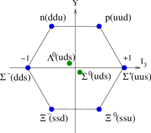
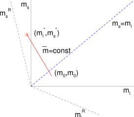
Figure 1: Left panel: The baryon octet in the $I_{3}$–$Y$ plane. Right panel: The path from the $SU(3)$-flavour symmetry line to the physical quark mass (denoted by a star). The axes for the renormalised quarks are non-orthogonal which depicts the situation for non-chiral actions, such as clover-Wilson fermions, [2].

The QCDSF strategy applied mainly to $2+1$ simulations (i.e. $\bar{m}_{u}=m_{d}\equiv m_{l}$) is to note that while there are many paths to approach the physical point, it is particularly favourable to extrapolate from a point on the $SU(3)$-flavour symmetry line, where all the quark masses are the same, to the physical point $(\bar{m}_{0},\bar{m}_{0})\longrightarrow(m^{*}_{l},m^{*}_{s})$ keeping the singlet quark mass $\bar{m}\equiv(2m_{l}+m_{s})/3$ constant, as illustrated in the RH panel of Fig. 1. This path is called the ‘unitary line’ as we expand in both sea and valence quarks.

Defining $\delta m_{q}=m_{q}-\bar{m}$ as the expansion paremter about the $SU(3)$-flavour symmetric point $\delta m_{q}=0$ then we find Taylor expansions which at low orders in $\delta m_{l}$ have constraints between the various octet masses. For example for the baryon octet we have

$$M_{N} = M_{0}+3A_{1}\delta m_{l}+\ldots$$

$$M_{\Lambda} = M_{0}+3A_{2}\delta m_{l}+\ldots$$

$$M_{\Sigma} = M_{0}-3A_{2}\delta m_{l}+\ldots$$

$$M_{\Xi} = M_{0}-3(A_{1}-A_{2})\delta m_{l}+\ldots\,.$$ (1)

This expansion is known up to and including $\delta m_{l}^{3}$ terms. Thus plotting the masses against $\delta m_{l}$, they fan out from the point $\delta m_{l}=0$. A further consequence is that singlet terms, such as $X_{N}=(M_{N}+M_{\Sigma}+M_{\Xi})/3=M_{0}+O(\delta m_{l}^{2})$ have no $O(\delta m_{l})$ terms. We shall find similar behaviour for the matrix elements.

2 Matrix element expansions

We now develop similar expansions for matrix elements given by

$$\langle B_{i}|J^{F_{j}}|B_{k}\rangle\equiv A_{\bar{B}_{i}F_{j}B_{k}}\,,$$ (2)

where our conventions are given in Table 1 for the possible

Index	Baryon ($B$)	Meson ($F$)	Current ($J^{\rm\scriptscriptstyle F}$)
1	$n$	$K^{0}$	$\bar{d}\gamma s$
2	$p$	$K^{+}$	$\bar{u}\gamma s$
3	$\Sigma^{-}$	$\pi^{-}$	$\bar{d}\gamma u$
4	$\Sigma^{0}$	$\pi^{0}$	$\frac{1}{\sqrt{2}}\left(\bar{u}\gamma u-\bar{d}\gamma d\right)$
5	$\Lambda^{0}$	$\eta$	$\frac{1}{\sqrt{6}}\left(\bar{u}\gamma u+\bar{d}\gamma d-2\bar{s}\gamma s\right)$
6	$\Sigma^{+}$	$\pi^{+}$	$\bar{u}\gamma d$
7	$\Xi^{-}$	$K^{-}$	$\bar{s}\gamma u$
8	$\Xi^{0}$	$\bar{K}^{0}$	$\bar{s}\gamma d$
0		$\eta^{\prime}$	${1\over\sqrt{3}}\left(\bar{u}\gamma u+\bar{d}\gamma d+\bar{s}\gamma s\right)$

Table 1: Our numbering and conventions for the generalised currents. For example, $B_{3}=\Sigma^{-}$, $F_{3}=\pi^{-}$, $J^{F_{3}}\equiv J^{\pi^{-}}=\bar{d}\gamma u$. We use the convention that current (i.e. operator) numbered by $i$ has the same effect as absorbing a meson with the index $i$. $\gamma$ represents an arbitrary Dirac matrix.

octet states, $i=1,\ldots,8$ and the singlet state, labelled by $i=0$ (which is considered separately). As we are primarily concerned with the flavour structure of bilinear operators, we use the corresponding meson name for the flavour structure of the bilinear quark currents. So for example the $i=5$ current is given by the flavour matrix $F_{\eta}=\mbox{diag}(1,1,-2)/\sqrt{6}$. We shall use the convention that the current $i$ has the same effect as absorbing a meson with the same index. As an example, we note that absorbing a $\pi^{+}$ annihilates one $d$ quark and creates a $u$ quark. That is $J^{\pi^{+}}|0\rangle\propto|\pi^{+}\rangle$. When $i\neq k$ we have transition matrix elements; when $i=k$ within the same multiplet, we have operator expectation values. This has already been indicated in Table 1.

In the case of $n_{f}=2+1$ flavours considered here we only need to give the amplitudes for one particle in each isospin multiplet, and can then use isospin symmetry to calculate all other amplitudes in (or between) the same multiplets. So, for example, we can calculate the $\Sigma^{-}$ and $\Sigma^{0}$ matrix elements if we are given all the $\Sigma^{+}$ matrix elements. Similarly, given the $\Sigma^{-}\to n$ transition amplitude, we can find all the other $\Sigma\to N$ transition amplitudes.

Within the set of amplitudes between baryons there are $7$ diagonal matrix elements: $A_{\bar{N}\eta N}$, $A_{\bar{\Sigma}\eta\Sigma}$, $A_{\bar{\Lambda}\eta\Lambda}$, $A_{\bar{\Xi}\eta\Xi}$ ($I=0$) and $A_{\bar{N}\pi N}$, $A_{\bar{\Sigma}\pi\Sigma}$, $A_{\bar{\Xi}\pi\Xi}$ ($I=1$) and $5$ transition amplitudes: $A_{\bar{\Sigma}\pi\Lambda}$ ($I=0$), and $A_{\bar{N}K\Sigma}$, $A_{\bar{N}K\Lambda}$, $A_{\bar{\Lambda}K\Xi}$, $A_{\bar{\Sigma}K\Xi}$ ($I=1/2$) giving $7+5=12$ in total. (There are a further $5$ inverse transition amplitudes, simply related to the previous $5$ transition amplitudes.) A Wigner-Eckart type theorem applies, the ‘reduced’ matrix element (or amplitude) being multiplied by a Clebsch–Gordan coefficient. For example $\langle p|J^{\pi^{+}}|n\rangle=\sqrt{2}\,A_{\bar{N}\pi N}=\sqrt{2}\;\langle p|J^{\pi^{0}}|p\rangle$ giving $\langle p|\bar{u}\gamma d|n\rangle=\langle p|(\bar{u}\gamma u-\bar{d}\gamma d)|p\rangle$. Further details and tables are given in [3].

Matrix elements follow the schematic pattern for 2+1:

$$\langle B_{i}|J^{F_{j}}|B_{k}\rangle = \sum(\mbox{singlet mass polynomial})\times(\mbox{singlet tensor})_{ijk}$$ (3)

$$+\sum(\mbox{octet mass polynomial})\times(\mbox{octet tensor})_{ijk}$$

$$+\sum(\mbox{27-plet mass polynomial})\times(\mbox{27-plet tensor})_{ijk}$$

$$+\sum(\mbox{64-plet mass polynomial})\times(\mbox{64-plet tensor})_{ijk}\,.$$

We already know the mass polynomials, [2], as given in the LH panel of Table 2.

Polynomial	$SU(3)$
$1$	$1$
$\delta m_{l}$		$8$
$\delta m_{l}^{2}$	$1$	$8$	$27$
$\delta m_{l}^{3}$	$1$	$8$	$27$	$64$

$SU(3)$	$T$, $1^{\rm st}$ class		$T$, $2^{\rm nd}$ class
	$d{\rm-like}$	$f{\rm-like}$	$d{\rm-like}$	$f{\rm-like}$
$1$	$d$	$f$
$8$	$r_{1}$, $r_{2}$, $r_{3}$	$s_{1}$, $s_{2}$	$t_{1}$, $t_{2}$	$u_{1}$
$27$	$q_{1}$, $q_{2}$	$w_{1}$, $w_{2}$	$x_{1}$	$y_{1}$
$64$	$z$

Table 2: Left panel: All the quark mass polynomials up to $O(\delta m_{l}^{3})$ classified by symmetry properties. Right panel: The relevant $17$ $T$-tensors, tabulated according to first/second class and $d$- or $f$-type.

So, for example, the $27$-plet part contains $O(\delta m_{l}^{2})$ and $O(\delta m_{l}^{3})$ terms. It remains to classify the $T_{ijk}=\langle B_{i}|J^{F_{j}}|B_{k}\rangle$ $3$-index tensors, $T_{ijk}$ and so need to look for a $SU(3)$ decomposition of $8\otimes 8\otimes 8$. Here we give a very brief sketch. We consider the tensor under $SU(3)$ rotations: $T^{\prime}_{ijk}=U^{\dagger}_{ia}T_{abc}U_{bj}U_{ck}$ and in particular the change in $T$ under an infinitesimal transformation by a generator $\lambda^{\alpha}$. Using isospin constraints and known Casimir eigenvalues (solving $512$ equations with Mathematica) imply that there are $17$ independent tensors with most $T_{ijk}$ elements zero or $\sqrt{\rm integer}$. These can then be further classified, by first defining a reflection matrix, $R$, which inverts the outer ring of the octet. The tensors can then be divided into first or second class depending on the symmetry

$${\rm first\ class\ \ \ } T_{ijk}=+T_{kai}R_{aj}\,,$$

$${\rm second\ class} T_{ijk}=-T_{kai}R_{aj}\,,$$

which interchanges $B_{i}$ and $B_{k}$ and transposes the flavour matrix $F^{j}$. This corresponds to the Weinberg classification of currents into first and second class, [6], as discussed in [3].

There is an additional classification by the symmetry when $R$ is applied to all three indices

$$d{\rm-like} T_{ijk}=+R_{ia}T_{abc}R_{bj}R_{ck}\,,$$

$$f{\rm-like} T_{ijk}=-R_{ia}T_{abc}R_{bj}R_{ck}\,.$$

We find eventually that there are $17$ tensors: two singlets, eight octets, six $27$-plets, one $64$-plet all contained in the $8\otimes 8\otimes 8$ decomposition. These are listed in the RH panel of Table 2.

We are now in a position to give the polynomial expansions of the amplitudes to $O(\delta m_{l}^{3})$. The same notation is used for the tensor and its coefficient. For example considering $\langle p|J^{\eta}|p\rangle\equiv\langle B_{2}|J^{5}|B_{2}\rangle=A_{\bar{N}\eta N}$ at say $O(\delta m_{l})$ we have from LH Table 2 that it is octet. From RH Table 2 we see that for first class, it can contain possible $r_{1}$, $r_{2}$, $r_{3}$ and $s_{1}$, $s_{2}$ tensor contributions. Checking which tensors have a non-zero $252$ component gives a coefficient $(r_{1}-s_{2})$.

Thus, as an example, we eventually find for a $1^{\rm st}$-class current

$$\langle p|J^{\eta}|p\rangle = A_{\bar{N}\eta N}$$ (4)

$$= \underbrace{\sqrt{3}f-d}_{1}+(\underbrace{r_{1}-s_{2}}_{8})\delta m_{l}$$

$$+(\underbrace{\sqrt{3}f^{\rm\scriptscriptstyle x}-d^{\rm\scriptscriptstyle x}}_{1}+\underbrace{r_{1}^{\rm\scriptscriptstyle x}-s_{2}^{\rm\scriptscriptstyle x}}_{8}+\underbrace{9q_{1}+3q_{2}+3\sqrt{3}w_{2}}_{27})\delta m_{l}^{2}$$

$$+(\underbrace{\sqrt{3}f^{\rm\scriptscriptstyle xx}-d^{\rm\scriptscriptstyle xx}}_{1}+\underbrace{r_{1}^{\rm\scriptscriptstyle xx}-s_{2}^{\rm\scriptscriptstyle xx}}_{8}+\underbrace{9q_{1}^{\rm\scriptscriptstyle x}+3q_{2}^{\rm\scriptscriptstyle x}+3\sqrt{3}w_{2}^{\rm\scriptscriptstyle x}}_{27}+\underbrace{3\sqrt{3}z}_{64})\delta m_{l}^{3}\,,$$

(by this we mean the relevant $1^{\rm st}$-class form factor) and as a further example for a $2^{\rm nd}$-class current

$$\langle n|J^{K^{+}}|\Sigma^{-}\rangle = A_{\bar{N}K\Sigma}$$ (5)

$$= (\sqrt{2}t_{2}+\sqrt{6}u_{1})\delta m_{l}+(\sqrt{2}t_{2}^{\rm\scriptscriptstyle x}+\sqrt{6}u_{1}^{\rm\scriptscriptstyle x}+\sqrt{5}x_{1}+\sqrt{2}y_{1})\delta m_{l}^{2}\,.$$

Complete tables are given in [3].

It is natural to ask what do we gain for all this effort. The answer is that the expansions are constrained, as can be easily ascertained by counting the available parameters. For $1^{\rm st}$-class currents there are $7+5=12$ possible amplitudes and we have from the RH panel of Table 2

• $O(1)$ has $2_{1}=2$ parameters

• $O(\delta m_{l})$ has $5_{8}=5$ parameters

• $O(\delta m_{l}^{2})$ has $2_{1}+5_{8}+4_{27}=11$ parameters

while at $O(\delta m_{l}^{3})$ we have $2_{1}+5_{8}+4_{27}+1_{64}=12$ parameters and $12$ amplitudes, so there are no further constraints. (The subscript denotes the representation given in the RH panel of Table 2.) Similarly for second-class currents – there are now $5$ possible amplitudes, the expansion starts at $O(\delta m_{l})$ and we have

• $O(\delta m_{l})$ has $3_{8}=3$ parameters

while at $O(\delta m_{l}^{2})$ we already have $3_{8}+2_{27}=5$ parameters, so again there are no further constraints. So in all cases we only have constraints at low orders in $\delta m_{l}$.

Alternatively we can construct linear combinations of amplitudes so that we have only $d$- or $f$-terms in the expansion. For example we have at $O(\delta m_{l})$ a $1^{\rm st}$-class $d$ expansion can be constructed

$$D_{1}\equiv-(A_{\bar{N}\eta N}+A_{\bar{\Xi}\eta\Xi}) = 2d-2r_{1}\delta m_{l}$$

$$D_{2}\equiv A_{\bar{\Sigma}\eta\Sigma} = 2d+(r_{1}+2\sqrt{3}r_{3})\delta m_{l}$$

$$D_{3}\equiv{}-A_{\bar{\Lambda}\eta\Lambda} = 2d-(r_{1}+2r_{2})\delta m_{l}$$

$$D_{4}\equiv\frac{1}{\sqrt{3}}(A_{\bar{N}\pi N}-A_{\bar{\Xi}\pi\Xi}) = 2d-\frac{4}{\sqrt{3}}r_{3}\delta m_{l}$$

$$D_{5}\equiv A_{\bar{\Sigma}\pi\Lambda} = 2d+(r_{2}-\sqrt{3}r_{3})\delta m_{l}$$

$$D_{6}\equiv\frac{1}{\sqrt{6}}(A_{\bar{N}K\Sigma}+A_{\bar{\Sigma}K\Xi}) = 2d+\frac{2}{\sqrt{3}}r_{3}\delta m_{l}$$

$$D_{7}\equiv-(A_{\bar{N}K\Lambda}+A_{\bar{\Lambda}K\Xi}) = 2d-2r_{2}\delta m_{l}$$ (6)

just as for the masses as in eq. (1) – a ‘$d$-fan’. We have $7$ lines, but only $3$ slope parameters, $r_{1}$, $r_{2}$, $r_{3}$, so the splittings are highly constrained. We can also construct quantities that are constant at $O(\delta m_{l})$, for example $X_{D}\equiv(D_{1}+2D_{2}+3D_{4})/6=2d+O(\delta m_{l}^{2})$. (These ‘averages’ are not unique, here we just use the diagonal terms.) Similarly for the $f$-fan: there are $5$ lines, but only $2$ slope parameters, $s_{1}$, $s_{2}$, so splittings are again highly constrained. Examples of ‘fan’ plots and ‘averages’ for the vector current are given in [3]. For a recent example for the tensor charge, see [7].

As a further example consider the renormalised vector current ($J^{r}\sim V_{4}$) at $Q^{2}=0$. This simply counts the quarks (positive) and anti-quarks (negative). So for the $7$ diagonal amplitudes, the results are constant and known. This gives

$$A_{\bar{N}\eta N}=\sqrt{3}f\,,\,A_{\bar{\Sigma}\eta\Sigma}=0\,,\,\,A_{\bar{\Lambda}\eta\Lambda}=0\,,\,\,A_{\bar{\Xi}\eta\Xi}=-\sqrt{3}f\,,\,\,A_{\bar{N}\pi N}=f\,,\,\,A_{\bar{\Sigma}\pi\Sigma}=2f\,,\,\,A_{\bar{\Xi}\pi\Xi}=f\,,$$ (7)

with $f=1/\sqrt{2}$, $d=0$. Note that because $d$ vanishes then $A_{\bar{\Sigma}\eta\Sigma}$ and $A_{\bar{\Lambda}\eta\Lambda}$ are identically zero. The vanishing of the $O(\delta m_{l})$ terms leads immediately to the vanishing of all the coefficients (i.e. $r_{1}$, $r_{2}$, $r_{3}$ and $s_{1}$, $s_{2}$). This then also implies that the $5$ transition matrix elements also have no $O(\delta m_{l})$ terms. This is the content of the Ademollo–Gatto theorem [8]. At the next order, $O(\delta m_{l}^{2})$, for the diagonal amplitudes we have $11$ parameters but $7$ constraint equations, so we can solve for $4$ parameters, which we take to be $q_{1}$, $q_{2}$, $w_{1}$, $w_{2}$. Substituting into the transition amplitudes gives

$$A_{\bar{\Sigma}\pi\Lambda} = 0+40\left(q_{1}-{1\over 3}q_{2}\right)\delta m_{l}^{2}$$

$$A_{\bar{N}K\Sigma} = -\sqrt{2}f+\left(5\sqrt{6}(q_{1}+q_{2})-5\sqrt{2}(w_{1}-w_{2})\right)\delta m_{l}^{2}$$

$$A_{\bar{N}K\Lambda} = -\sqrt{3}f+\left(5(q_{1}-{5\over 3}q_{2})+5\sqrt{3}(w_{1}+{1\over 3}w_{2})\right)\delta m_{l}^{2}$$

$$A_{\bar{\Lambda}K\Sigma} = \sqrt{3}f+\left(5(q_{1}-{5\over 3}q_{2})-5\sqrt{3}(w_{1}+{1\over 3}w_{2})\right)\delta m_{l}^{2}$$

$$A_{\bar{\Sigma}K\Xi} = \sqrt{2}f+\left(5\sqrt{6}(q_{1}+q_{2})-\sqrt{2}(w_{1}+w_{2})\right)\delta m_{l}^{2}\,.$$ (8)

So we have one constraint between the $5$ amplitudes at $O(\delta m_{l}^{2})$.

We finally note that to complete the job to determine all expansions, we also need the singlet $\eta^{\prime}$ as given in Table 1. For example for $\bar{u}\gamma u=J^{\eta^{\prime}}/\sqrt{3}+J^{\pi^{0}}/\sqrt{2}+J^{\eta}/\sqrt{6}$ (and similarly for $\bar{d}\gamma d$, $\bar{s}\gamma s$) we need the singlet i.e. $A_{\bar{N}\eta^{\prime}N}$. But these expansions are $8\otimes 1\otimes 8$ and so have already been determined by the mass expansions [2]. For example from eq. (1) we have $A_{\bar{N}\eta^{\prime}N}=a_{0}+3a_{1}\delta m_{l}+\ldots$ which allows for example $\langle p|\bar{u}\gamma u|p\rangle$ to be determined. This construction is necessary for example for the electromagnetic current. Again see [3] for more details.

3 Numerical results

We consider $2+1$ Symanzik tree-level, $O(a)$ improved clover fermions, [9] at $\beta=5.50$, where $a\sim 0.074\,\mbox{fm}$. At the flavour symmetric point $M_{\pi}\sim 465\,\mbox{MeV}$.

For the vector current ($J\sim V_{4}$) we have determined the $12$ $F_{1}$ form factors (amplitudes) at $Q^{2}=0$ (using twisted boundary conditions for the transition amplitudes to achieve this) on a $24^{3}\times 48$ lattice. Our preliminary results (for $5$ quark masses) are given in Fig. 2.

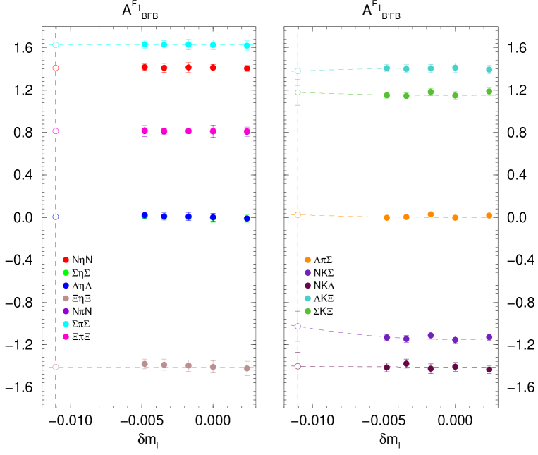
Figure 2: Left panel: The $7$ diagonal $F_{1}$ amplitudes together with fits as described in the text. The filled points denote the numerical data, while the open points are at the physical pion mass. $\delta m_{l}=0$ is the $SU(3)$-flavour symmetric point. Right panel: The $5$ transition $F_{1}$ amplitudes.

Note that on the $\bar{m}=\mbox{const.}$ trajectory we have also a data set with a light strange quark mass and a heavy light quark mass.

In the LH panel we show the diagonal amplitudes for $F_{1}$ and in the RH panel the transition amplitudes also for $F_{1}$, together with a joint constrained fit given by eqs. (7), (8). As expected first for the diagonal amplitudes the numerical data is very constant (i.e. independent of the quark mass), which the fit reproduces. Also as the renormalised value of $f$ is $1/\sqrt{2}$, then presently ignoring any $O(a)$-improvement, gives an estimate of the multiplicative vector renormalisation constant, $Z_{V}$. As $A_{\bar{\Sigma}\eta\Sigma}$ and $A_{\bar{\Lambda}\eta\Lambda}$ are identically zero (i.e. have a zero fit function) we fit these separately with a constant, which gives a consistency check of the data.

Turning now to the RH panel of Fig. 2 we show the transition amplitudes for $F_{1}$. The joint constrained fits are given by eq. (8). We find little evidence of discrepancies from the leading order, LO, constant values, except possibly for $A_{\bar{N}K\Sigma}$. However as the fit coefficients presently have large uncertainties then it is really necessary to extend the computation to smaller quark masses, before any conclusion can be reached. It is interesting to note that [10] finds some evidence for discrepancies from the LO value for both $A_{\bar{N}K\Sigma}$ and $A_{\bar{\Sigma}K\Xi}$, however they both increase the absolute value of the amplitudes.

4 Conclusions

In this talk we have discussed baryon octet $SU(3)$-flavour symmetry breaking expansions for matrix elements (parallel to the previous mass expansions) for $2+1$ quark flavours. This is complementary to chiral expansions which start at a numerically out-of-reach zero quark mass, rather than here where we start at the $SU(3)$-flavour symmetry point. As for the mass case we again find constrained expansions. As an example, we have indicated that it might be possible to investigate discrepancies from the vector current LO values for the baryon octet at $Q^{2}=0$. Among various future extensions, one possibility is to consider the meson octet.

References

- [1] W. Bietenholz et al., Phys. Lett. B 690 (2010) 436, [arXiv:1003.1114 [hep-lat]].
- [2] W. Bietenholz et al., Phys. Rev. D 84 (2011) 054509, [arXiv:1102.5300 [hep-lat]].
- [3] J. M. Bickerton et al., Phys. Rev. D 100 (2019) 114516, [arXiv:1909.02521 [hep-lat]].
- [4] R. Horsley et al., J. Phys. G 43 (2016) 10LT02, [arXiv:1508.06401 [hep-lat]].
- [5] R. Horsley et al., JHEP 04 (2016) 093, [arXiv:1509.00799 [hep-lat]].
- [6] S. Weinberg, Phys. Rev. 112 (1958) 1375.
- [7] R. Smail et al., “Tensor Charges and their Impact on Physics Beyond the Standard Model”, LATTICE2021, 26th-30th July 2021.
- [8] M. Ademollo et al., Phys. Rev. Lett. 13 (1964) 264.
- [9] N. Cundy et al., Phys. Rev. D 79 (2009) 094507, [arXiv:0901.3302 [hep-lat]].
- [10] S. Sasaki, Phys. Rev. D 96 (2017) 074509, [arXiv:1708.04008 [hep-lat]].
- [11] T. R. Haar et al., EPJ Web Conf. 175 (2018) 14011, [arXiv:1711.03836 [hep-lat]].
- [12] R. G. Edwards et al., Nucl. Phys. B Proc. Suppl. 140 (2005) 832, [arXiv:hep-lat/0409003 [hep-lat]].