SoK: Vehicle Orientation Representations for Deep Rotation Estimation

Abstract

In recent years, there is an influx of deep learning models for 3D vehicle object detection. However, little attention was paid to orientation prediction. Existing research work proposed various vehicle orientation representation methods for deep learning, however a holistic, systematic review has not been conducted. Through our experiments, we categorize and compare the accuracy performance of various existing orientation representations using the KITTI 3D object detection dataset [1], and propose a new form of orientation representation: Tricosine. Among these, the 2D Cartesian-based representation [cos($\theta$), sin($\theta$)], or Single Bin, achieves the highest accuracy, with additional channeled inputs (positional encoding and depth map) not boosting prediction performance. Our code is published on GitHub: https://github.com/umd-fire-coml/KITTI-orientation-learning

1 Introduction

Within vehicle object detection tasks, rotation estimation typically receives little attention, due to the main tasks, object localization and dimension estimation, receiving more focus. We believe that finding ways to improve orientation estimation is an important task, because accurate orientation estimation is useful for dependent tasks such as path projection [2, 3, 4], birds-eye-view visualization [5, 6, 7, 8], and dimensions estimation [9, 10, 11].

However, accurate rotation estimation contains challenges that seems to be highly dependant on the rotation representation target for deep learning. With the default angle representations in radians/degrees (based on either global or local camera angle), the problem of discontinuity occurs when rotation values $\theta\in[-\pi,\pi]$ circularly jump from $-\pi$ to $\pi$, potentially resulting in huge losses for small angle changes across the wrap around boundary.

Some existing literature aim to solve this problem by mapping $\theta$ in a cosine or sine function, that can provide a circular, continuous representation while maintaining the compactness of one output value. However, using this alone creates an ambiguity problem, where cos($\theta$) and sin($\theta$) values now map to two $\theta$ values within [-$\pi$,$\pi$].

Discontinuity and ambiguity can be solved with a 2-D Cartesian representation using (cos($\theta$), sin($\theta$)) pair, creating a continuous, unambiguous representation [12] for every $\theta\in[-\pi,\pi]$. Some representations further this approach, treating this pair as a sub-component of a larger representation by dividing the [-$\pi$,$\pi$] range into equal sized ”bins” and isolating the orientation representation to a fixed range [13]. A research paper further extends this multiple bins representation by adding a component representing a confidence value on top of the (cos($\theta$), sin($\theta$)) pair values within each bin [14].

However in 2021, much of the existing Vehicle Object Detection research selects one of various rotation representations for prediction without much cited test results or numerical evidence for their choice. Current literature has more than 5 ways to represent a vehicle’s rotation without a clear unified message of which is the best way for representation, and whether switching to different representation could affect prediction accuracy.

Hence, our work aims to provide numerical results for the most accurate type of vehicle orientation representation, in hope that future object detection work will cite this evidence. We implemented various type of orientation representations and compared their results. For every type of orientation representation, we used a similar backbone and training setup, with the only variable being the final output layer to represent the vector that corresponds to the component values for the type of orientation representation.

We also extend our analysis with additional inputs such depth map and positional encoding, to see if providing depth and localization information results in improved performance respectively.

This process can be easily replicated to more complicated orientation representations with more rotational axes, other inputs like LiDAR or stereo images, and other datasets.

With this systematization of knowledge paper we make the following contributions:

• Develop a process for testing various types of vehicle orientation representation.

• Categorize and clarify various commonly used orientation representations.

• Train and evaluate different types of representations for accuracy and complexity.

• Discuss why among these, 2-D Cartesian representation is the best type of representation for deep rotation estimation.

2 Vehicle Orientation Representations

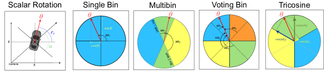
Figure 1: A visualization of the presented orientation methods

2.1 1-D Scalar Representations

Orientation representations in this section measure an object’s orientation as the rotational offset between the angle and a camera reference axis, in radians or degrees. These representations benefit from compactness, representing orientation with a single scalar value, which can reduce the model’s final output layer to a single node. However, Grassia [15] states that Euler angles and quaternions representation[16] are not ideal to compute and differentiate positions, due to the discontinuity [17] and ambiguity problem. We still observe recent researchers such as [18, 19, 20, 21, 22, 23, 24, 25, 26, 27, 28, 29, 30] using these types of scalar-based angle representation in 3D Object Detection. We are also noticing some variants of the scalar-based methods. Wang et al. [31] claimed better performance when dividing the angles into 2-bins with each bin represented by angle $\theta$ (offset) with period $\pi$ to distinguish two opposite orientations, but such method suffer from the discontinuity and ambiguity problem for values at the border of each bin. Shrivastava and Chakravarty [32] normalized orientation angle to (0,1). Carrillo and Waslander [33], Gahlert et al [34], and Plaut et al [35] studied the multiple degrees of freedom rotation of vehicle by applying regressing on scalar Euler angle independently on each axis.

However, all 1-D scalar-based orientation representation suffer from non-continuity [12], where model predictions near the boundary of the orientation’s range can result in an extreme loss even if the angular prediction is close to the ground truth, e.g. a 2$\pi$ rad prediction and 0 rad ground truth incurs an extremely large loss for the prediction, when using L1/L2 loss.

Some previous works attempts to alleviate the non-continuity problem [36] by having a customized loss function based on the 2D angular difference instead of the L1/L2 distance on the scalar value. However, these loss functions are not converging between prediction and ground truth angles that are exactly $\pi$ radians apart since they have near-zero gradient values.

It also needs additional considerations to ensure that it penalizes out-of-bound scalar prediction values, such as for values below $-\pi$ or above $\pi$. The loss function should not simply use 2D angular difference for loss as it would be able to correct extreme scalar prediction values.

A customized loss function is also prone to implementation errors, as it needs to be compatible with the automatic differentiation engine of machine learning frameworks (e.g. tensorflow and pytorch). It also require re-implementation and testing for each specific framework, unlike common loss functions such as L1/L2 loss.

2.1.1 Rotation-Y (Global/Egocentric Rotation)

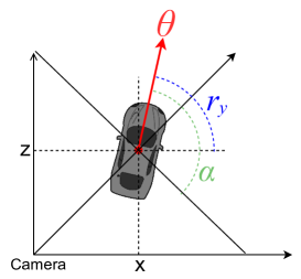
Figure 2: The $r_{y}$ and $\alpha$ radial observation angle forms given by KITTI. The $\alpha$ representation contains the car’s appearance to the camera, while $r_{y}$ depicts the vehicle relative to the scene.

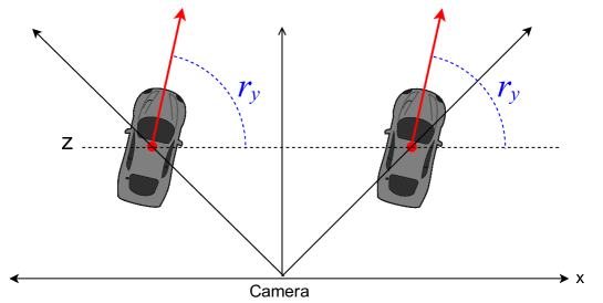
Figure 15: Example of radial angle form Rotation Y held constant. The vehicle’s orientation now does not depend on what the camera sees, but rather the orientation of the vehicle within the scene.

Rotation-Y, $r_{y}$, also know as camera z-axis rotation or egocentric global rotation [1, 37], is one of two orientation representations given in KITTI object detection labels [1]. It measures the object’s orientation in radians ($r_{y}$ $\in[-\pi,\pi]$), relative to the axis perpendicular to the camera’s forward facing z-axis. Two objects with the same $r_{y}$ value will point in the same direction relative to the scene regardless of the camera location. See Figure 15 for changes that can occur with constant global rotation.

2.1.2 Alpha (Local/Allocentric Rotation)

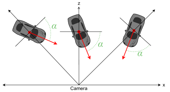
Figure 14: Example of radial angle form $\alpha$ held constant. Observe that the vehicle will have the same appearance to the camera from the shown locations.

Alpha, $\alpha$, also known as the local observation angle of the object, is another scalar orientation representation provided in the KITTI object detection labels [1]. It measures the object’s orientation in radians ($\alpha\in[-\pi,\pi]$), relative to camera’s observation angle towards the center of the object. Figure 2 provides a bird’s eye view visual representation of how $\alpha$ is measured. See Figure 14 for visual examples of changes that can occur with constant local rotation.

Two objects with the same $\alpha$ value will have a similar visual appearances [38], e.g. car headlights directly facing the camera (see Figure 14). Therefore, it may be easier for a model to learn to predict the $\alpha$, given the camera local appearance of an object. However, because camera sensors are usually flat (not curved to keep a constant focal distance) [39], optical distortions at different frame positions, e.g. an object near the edge of the frame vs an object at the center of the frame, can produce varying camera observed distorted appearances despite having same $\alpha$ values.

To draw and visualize a object’s orientation from a bird’s eye view perspective, the object’s $\alpha$ will need to be converted into $r_{y}$. With the object’s x and z location information, we can convert $r_{y}$ to $\alpha$ or vice versa [40, 41, 42], using the formula:

$$r_{y}=\alpha+\arctan\frac{x}{z}$$ (1)

where $x$ represents the object’s horizontal position, and $z$ represents the object’s forward distance, both relative to the center of the camera.

2.2 Single Bin (2-D Cartesian Representations)

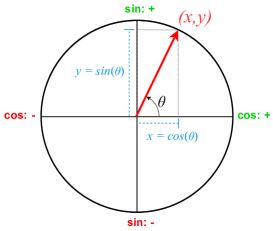
Figure 3: A reference displaying the mapping from angles to Cartesian coordinates

The discontinuity problem can be partly resolved by representing the angle using the cosine of the angle [43, 44, 45, 46, 47] or sine of the angle [48, 49] only due to its periodic properties. However, only using one of the cosine and sine of the angle cannot be unambiguously converted back into the angle without using at least 3-bins. Furthermore, when the angular difference is $\delta=\pm\pi$, the differentiation results of such angle, i.e. $cos(\delta)$, are zero, which could stop backpropagation learning at the extreme opposite output. To resolve this problem, researchers [50, 51, 52, 53, 54, 55, 56, 57, 58, 59, 60, 61] performed regression on both the cosine and sine of the angle (cos($\theta$), sin($\theta$)). When converting any given 1D Scalar-Based Orientation $\theta$ into 2-Dimensional values, they can be mapped to 2-D Cartesian system with angle’s cosine value projected to x-axis and sine value projected to y-axis. [62] Figure 3 provides a visual representation of how the 2D Cartesian representation of an object’s orientation is measured.

2D Cartesian-based representation can be unambiguously converted back into $\theta$ in radians using the formula:

$$\theta=\arctan\frac{cos(\theta)}{sin(\theta)}$$ (2)

This type of angle representation avoids the non-continuous boundary problem in 1-D Scalar-Based methods, allowing a model to use L1/L2 loss to penalize on the angular difference while also penalizing out-of-bound predictions, creating a smooth gradient for convergence, unlike singular value representations. However, even with L1/L2 loss during training, model predictions can still make out-of-bound values, so additional post-processing is needed to clip or scale the predicted values within the valid cosine and sine ranges.

2.3 N-Bin and Affinity Representations

The discontinuity issue can also be resolved by converting the angle $\theta$ into a discrete classification problem, by using multiple confidence values to represent the affinity for each bin. This generalizes to any other methods where the highest value first determines what bin the angle lies in. We dub these as Affinity based representations. Liao et al. [63] stated that converting the angle to discrete classification forms lead to stable training and convergence. Using discrete bins has a potential trade-off between the number of bins that leads to longer training time due higher number of final layer nodes and the prediction accuracy, so final angle prediction accuracy depends on the number of bins and specific implementations[63]. Researchers [64, 65, 66] first predict on a few discrete bins and then regress on the offset. There are also works designed to utilize a large number of bins or more exotic techniques: 12 non-overlapping equal bins [67], 72 non-overlapping bins [68], mean-shift after binning twice [36].

However, it is important to reduce the number of parameter in representing the rotation as the number of parameters directly affect the number of node in the final output layers. There are also complications in combining loss functions, as it creates loss competitions and non-smooth loss gradients, resulting in convergence issues during training. For these reasons, we selected to test the most commonly used techniques.

2.3.1 Multibin [14]

Figure 4: Multibin based representation. Each bin is encoded with a 2-D Cartesian value pair (or Single Bin) and a confidence value. Offset and non-offset cases provide differing bin/confidence values to create a more continuous form [14].

Multibin attempts to approach orientation estimation by classifying a bin with the highest confidence values and overlapping bins. Mousavian et al.[14] poses that the model should predict a confidence vector to first classify one bin, then reverse this bin’s sine, cosine value pair. The authors have outstanding performance with only two bins, utilizing a 10% total overlap at the bins’ borders, see Fig.4. This overlap assists with identifying angles close to the edge of these bins, which is elaborated upon later. Multiple papers [69, 70, 71, 72, 73, 74, 75, 76, 77, 78, 79, 80, 81, 82, 83, 84, 72] utilize this technique. The diagram 4 shows the angle, from each bin start to the angle.

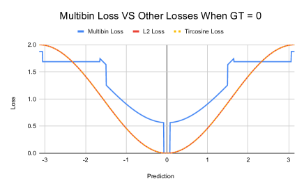
Figure 5: Graph of loss value for Multibin Loss, L2 losses and Angular Loss when the ground truth is set to zero radians. i.e. let $\theta_{gt}$ be the ground truth, $\theta_{pred}$ be the predicted value and $loss$ be the loss function. For all $\theta_{pred}\in[-\pi,\pi]$ hypothetical predicted outputs, we convert them into their corresponding orientation representations using the conversion algorithm $C$, and then plot $loss(C(\theta_{pred}),C(\theta_{gt}=0))$.

In Figure 5, we explore the smoothness of different loss functions. Angular loss overlaps with the l2 loss. For multibin [14], although the graph indicates lowest loss at zero, multibin does not have a smooth loss function. When the predicted value is within around $[\frac{1}{2}\pi,\pi]$, the gradient of loss function is zero, which gives no feedback to the model and traps them in local minimum.

To signal which bin the angle $\theta$ lies, it assigns a confidence value to each bin’s Cartesian pair values. Labels are given confidence values as follows. A confidence value of 1.0 means $\theta$ lies in that bin and not within the overlap region, while 0.0 confidence means $\theta$ does not lie in that bin. For $\theta$ within the overlapping region, a confidence of 0.5 is given to each overlapping bin.

Multibin also labels each bin with cos($\Delta\theta$) and sin($\Delta\theta$), where $\Delta\theta$ is the angular distance to the bin’s starting edge, i.e. offset. For the overlapping case, when $\theta$ is inside any overlapping region, both bins are given the cosine and sine values of each bin’s respective offset. For the non-overlapping case, the bin containing $\theta$ receives the cosine and sine of the offset, while the other bin is given all zeros.

Hence, Multibin attempts to use both the 2-D Cartesian and N-D affinity values in the representing the final orientation. However, this approach make it difficult to use a simple L1/L2 loss. A custom loss function will be needed to take into 0/1 confident predictions and 0.5/0.5 confident affinity predictions for overlapping bins. Additionally, we have found overlap prevents convergence, so we remove it and call this simpler form Confidence Bin.

2.3.2 Voting Bins

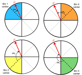
Figure 6: Voting bin based representation. Each bin is encoded with a 2-D Cartesian value pair (or Single Bin). Modeled after Multi-bin without confidence, the bins’ values are averaged after the voting/exclusion algorithm.

Zhao et al [13] proposes FFNet requiring 3 or more bins, instead of explicitly using confidence values for averaging, to unambiguously convert it back into a 1-D representation. Each bin’s values encode the angular offset $\Delta\theta$ from the middle of each bin (instead from the start of each bin). The original author recommends 4 bins. Converting back to a 1-D representation is an average of all candidate bin’s reversed offset angles, where any heavily outlying bins are ”voted” out or excluded from the average by the algorithm below:

If any bin meets both conditions below, they are voted out of the averaging.

• It and all other bins’ difference are below a fixed threshold (30 degrees)

• All other bins’ difference are also below the threshold (dynamic)

2.3.3 Tricosine

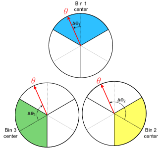
Figure 7: The Tricosine representation encodes the input angle with three cosine values. This allows for bin classification and regression within a continuous representation. This comes from the highest cosine value providing the bin center to create an average.

Unlike the previous methods, Tricosine aims to encode an angle in radians into the minimum number of bin affinity values that can unambiguously converted back into radians, i.e three. It utilizes three bins, each containing the cosine of the angular offset to each bin’s center.

Converting back a singular angle displays the affinities’ natural hierarchy. The highest affinity value first determines what bin the angle lies in. The inverse cosine of each affinity provides a relative position for our angle, where we utilize the other affinities’ inverted values to sway our prediction, further supplying accuracy. This swaying is a simple mean of each inverted affinity value, relative to the classified bin.

3 Model and Training Setup

3.1 Dataset

As a widely used benchmark for many visual tasks including 2D Object detection, Bird’s Eve View (BEV) tasks, depth estimation, and 3D object detection, the KITTI dataset [1] contains 7481 training images and 7513 testing images captured by the stereo camera and LiDAR sensors. Each instance is labeled with 2D and 3D bounding box location, 3D bounding box dimensions, orientation in $\alpha$ (alpha) and $r_{y}$ (rotation y). Other values are not used in our analysis. As an assumption of the KITTI dataset, vehicles only rotate with respect to the yaw axis, known as canonical orientation, so vehicle instances are always on a flat road instead of climbing a ramp. Scenes are restricted to highways and rural areas.

3.2 Data Preprocessing

In data prepossessing, we applied horizontal flipping image augmentation with the probability of 0.5 to the cropped image[81], and then converted the orientation labels to the different prediction representations. For example, before training the Voting Bin model, we convert the rotation y angles into four discrete bin affinity values.

All instances are cropped with their 2D bounding box and resized to 224x224. For feature extraction, we use Xception Net[85] as our backbone, achieving a good balance between model size and accuracy[86]. In the final output layers, two fully connected layers are used, with 1024 and N-D output nodes respectively.

3.3 Model Architecture

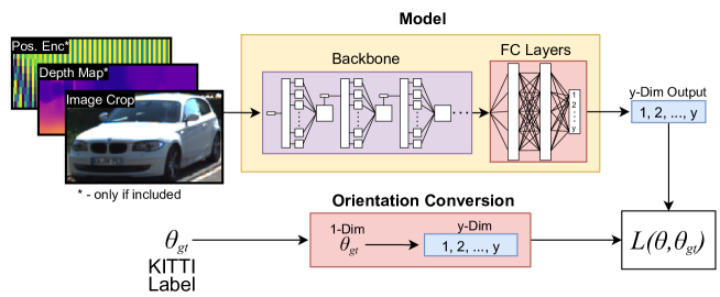
Figure 8: Illustration of Model and Training Process

Our contributions include comparison of these angular representations to monocular image inputs and the ’Car’ class to remove potential geometric shortcuts gained from LiDar and stereo imagery and prevent a cost competition between classes [13] respectively.

3.4 Loss Functions

We used simple mean squared error (L2 loss) as the loss function for all of the training experiments except for experiment E2.

$$L(\hat{\theta},\theta)=(\hat{\theta}-\theta)^{2}$$ (3)

Here ${\hat{\theta}}$ is the prediction vector, and $\theta$ is the ground truth vector after converting to the corresponding angle representation.

Following [87], we also consider an angular loss form to train on 1-D global rotation, or $r_{y}$. The angular loss function focuses only on the angular differences between angles, whereas the L2 loss computes the mean squared error on the scalar value differences for each component in the angle representation vector, which considers the norm of the vector representation and introduces the scalar discontinuity problem (see section 1).

Angular loss function can be expressed as:

$$L(\theta,\hat{\theta})=1-\cos(\theta)=1-\frac{\hat{\theta}\cdot\theta}{|\hat{\theta}||\theta|}=1-\frac{x_{g}x+y_{g}y}{\sqrt{x^{2}+y^{2}}}$$ (4)

Here $\hat{\theta}=[x,y]$ is the predicted vector, where $x=cos(\hat{\theta})$, $y=sin(\hat{\theta})$, and $\theta=[x_{g},y_{g}]$ is the ground truth vector, where $x_{g}=cos(\theta),y_{g}=sin(\theta)$.

3.5 Accuracy Metric

For all prediction methods, we compute the Orientation Similarity (OS) metric as provided by KITTI [1] without recall consideration. The cosine-like orientation similarity metrics computes the accuracy of predicted and ground truth angles in 1-D scalar representation, and maps the prediction and ground truth cosine distance to between [0, 1].

$$OS({\hat{\theta}},{\theta})=\frac{1}{N}\sum_{i=1}^{N}\frac{1+cos(\hat{\theta_{i}}-\theta_{i})}{2}$$ (5)

3.6 Training Setup

We train our model using prediction methods, Global Rotation ($r_{y}$), Local Rotation ($\alpha$), Single Bin, Tricosine, Voting Bin, and Confidence Bins to predict one of two targets: global rotation ($r_{y}$) and location rotation ($\alpha$). Our models were first trained on a Nvidia V100 GPU for 1-D scalar based representation experiments and later on a Nvidia RTX3090 GPU for all other experiments. All models were trained with TensorFlow’s default Adam optimizer [88] (lr= 0.001, $\beta 1$= 0.9, $\beta 2$= 0.99, $\epsilon$= 1e-7), a batch size of 25, and 100 total epochs.

4 Experiment Results Discussion

In the section, we will provide a discussion on the key findings of our experiments. An overview of our experiment results is provided in table 1.

Exp ID	Prediction Method	Loss Functions	Additional Inputs	Accuracy (%)
E1	Global Rot	L2 Loss	-	90.490
E2	Global Rot	Angul. Loss	-	89.052
E3	Local Rot	L2 Loss	-	90.132
E4	Single Bin	L2 Loss	-	94.815
E5	Single Bin	L2 Loss	Pos Enc	94.277
E6	Single Bin	L2 Loss	Dep Map	93.952
E7	Voting Bins	L2 Loss	-	93.609
E8	Tricosine	L2 Loss	-	94.249
E9	Tricosine	L2 Loss	Pos Enc	94.351
E10	Tricosine	L2 Loss	Dep Map	94.384
E11	2 Conf Bins	L2 Loss	-	83.304
E12	4 Conf Bins	L2 Loss	-	88.071

Table 1: Experiment result overview

4.1 1-D Global vs. 1-D Local Representation

Based on experiments E1 and E3, we compare two types of orientation representations in 1-D, global and local rotation representations, to answer: Which is a better prediction target in 1-D scalar orientation representation?

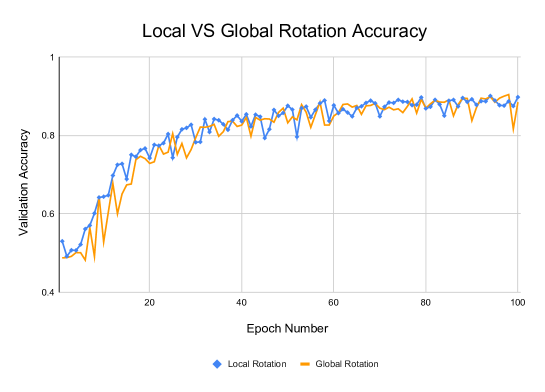
Figure 9: Max Validation accuracy of 1-D Global and local representation after 100 epochs of training.

Target	Accuracy (%)
Global Rotation	90.490
Local Rotation	90.132

Table 2: Validation accuracy of training with 1-D Global and 1-D Local representation across 100 epochs of training.

To answer this question, we initialized two models with the same backbone and output layers. We normalized target values to [-1, 1] from the dataset’s range of [$-\pi$ and $\pi$]. The loss function used for both models during training was L2.

The training results, in table 2, show that the difference in the highest validation accuracy of 1-D Global and Local rotation is small, around 0.5% after 100 epochs of training, which is within the margin of error between epochs. We conclude that there is either no difference or a slight disadvantage in using Local representation compared to using global representation.

Thus, we speculate that the network is capable of detecting the global/egocentric orientation of an object using without needing the conversion into an angle based on the direction of camera observation.

4.2 Angular Loss vs L2 loss

While angular loss removes the inherent radial length of single bin outputs by normalizing the bin’s output, there are notable drawbacks that L2 does not encounter. For instance, angular loss’s gradient encounters zeros within the prediction range [-2$\pi$, 2$\pi$], so an exact prediction of $\theta\pm\pi$ from ground truth will have no gradient to train the model’s weights. Likewise, predictions near $\theta\pm\pi$ will suffer from diminished gradients and take a long time to converge.

Since angular loss does not penalize the radial length of the output, we expected to have unbounded outputs paired with low loss. However, according to table 3, there was only little performance drop when using angular loss function. The batch-normalization layer [89] may explain this, as it clips the value range in case of output explosion and stabilize the training process. This can also be clamped at the model’s output with a softmax layer, but this requires further testing. We do not believe it is necessary due to the low performance differences.

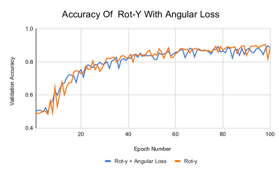
Figure 10: Validation Accuracy of prediction method Global Rotation with and without angular loss.

Method	Loss Function	Accuracy (%)
Global Rotation	MSE	90.490
Global Rotation	Angular Loss	89.052

Table 3: Highest validation accuracy using two different loss function. Prediction target and prediction method are both Rotation Y

4.3 1-D vs. 2-D vs. N-D Bin Affinity Representation

We compare three types of orientation representations in 1-D, 2-D, 3-D, 4-D, and 8-D to answer the research question: Which vector dimensions of angle representation improve prediction accuracy?

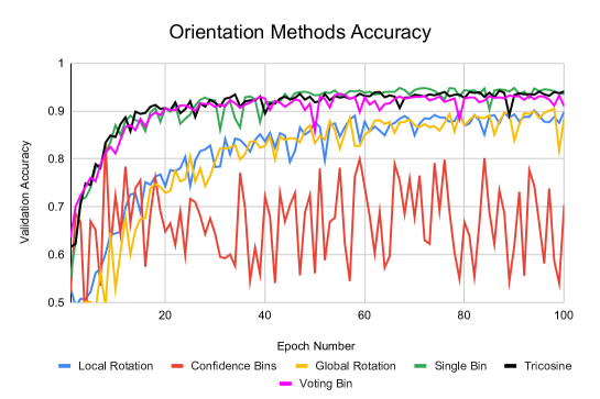
Figure 11: Max Validation accuracy of 1-D, 2-D, 3-D, 4-D, 8-D representation after 100 epochs of training.

Target	Method	Accuracy (%)
1-D	Global Rotation	90.490
1-D	Local Rotation	90.132
2-D	Single Bin	94.815
3-D	Tricosine	94.249
4-D	Confdence Bins	83.304
8-D	VotingBin	93.609

Table 4: Highest validation accuracy on 5 prediction methods with prediction target of rot-y.

Performance is measured by validation accuracy per epoch, which immediately divides into three groups with Single Bin, Tricosine, and Voting Bin performing the highest. Followed by the next performance group, global and local representation, these two groups display expected performance differences, as 1-D angular representation contains the challenge of discontinuity while Single Bin, Tricosine, and Voting Bin have compact, continuous representations. The third group contains Confidence Bin, which performs better than Multibin, but does not converge to the other N-D based methods.

4.4 Positional Encoding

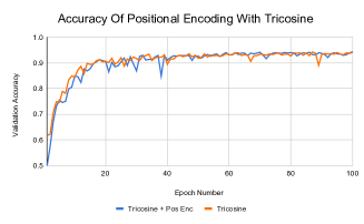
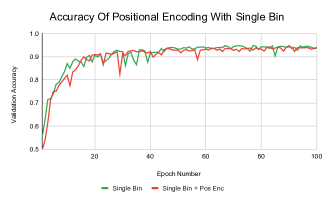
Figure 12: Validation accuracy comparison between models with and without the positional encoding layer appended to input across 100 epochs.

Target	Additions	Accuracy %
Single Bin	-	94.815
Single Bin	PosEnc	94.277
Tricosine	-	94.249
Tricosine	PosEnc	94.351

Table 5: Highest validation accuracy comparison between models with and without positional encoding layer.

As only image crops are inputted to the network, we observe that crops’ positions are ambiguous. Inspired by transformers [90], we concatenate [91, 92, 93, 94, 95, 96] a positional encoding channel to the RGB input and feed them as 4-channel images into the network. We hope to provide the crop’s positional information to the model, and thus improve the $r_{y}$ accuracy. However, as shown in Table 5, positional encoding provides little gain when predicting against $r_{y}$. We are not sure about the exact reason. Still, we speculate that the model either ignores the added channel or can estimate the position to some extent via the distortion[97] of the object within the crop.

4.5 Depth Map + Image Crop vs. Image Crop Only

Similar to adding positional encoding to input, we want to test if the model can perform better if more depth information is provided. We generated depth maps for all RGB inputs with LapDepth model [98] in advance, and concatenated[99, 100, 101] them to the RGB images as input, which then is fed into the network. As listed in the table 6, we don’t see any statistically significant improvement in accuracy. There is no solid explanation of it but we hypothesize that the model has the ability to estimate the depth of objects in the image.

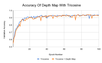
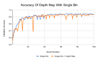
Figure 13: Validation accuracy comparison between models with and without the positional encoding layer appended to input across 100 epochs.

Target	Concatenations	Accuracy %
Single Bin	-	94.815
Single Bin	depth map	93.952
Tricosine	-	94.249
Tricosine	depth map	94.384

Table 6: Highest validation accuracy comparison between models with and without depth map in input.

5 Conclusion

In this work, we performed extensive experiments on three types of orientation representations: 1-D scalar, 2-D Cartesian, and N-D bin affinity representations. We found that Single Bin with 2-D Cartesian representation achieved the highest accuracy. We also proposed and tested a novel way of predicting 3D orientation: Tricosine which achieves second-to-the-best validation accuracy. Although multiple existing works implement the Multibin representation, we found that it did not perform well, potentially because of its unsmooth loss function. Confidence Bins has much greater performance than Multibin as it has a smooth loss function, but it did not perform as well as Tricosine or Single Bin with 2-D Cartesian representation.

These results concretely confirm other works’ conclusion regarding the problem of non-continuity in scalar representation, as the representations with continuous and unambiguous representations such as Single Bin, Tricosine, and Voting Bin all achieved the greater performance than scalar representation.

Additionally, we found that using local rotation targets did not outperform global rotation targets. This was surprising as we expected global rotation to perform poorly due to the major visual differences between crops of constant global rotation. We also tested if assisting the image crops with the location of the crop within the image can have improved performance, by adding positional encoding. However, our results from adding positional encoding to predict global rotation target gained little performance, and at times destabilized validation accuracy across training epochs.

Our work was limited in using only monocular object image crops as inputs. Perhaps lidar-based and multi-camera inputs may provide further improvements to the orientation estimation tasks. We look to future work to see if our methods also apply to full 3-DoF rotation and other orientation representation methods.

6 Appendix

References

- [1] Andreas Geiger, Philip Lenz and Raquel Urtasun “Are we ready for autonomous driving? The KITTI vision benchmark suite” ISSN: 1063-6919 In 2012 IEEE Conference on Computer Vision and Pattern Recognition, 2012, pp. 3354–3361 DOI: 10.1109/CVPR.2012.6248074
- [2] Y. Alon, A. Ferencz and A. Shashua “Off-road Path Following using Region Classification and Geometric Projection Constraints” In 2006 IEEE Computer Society Conference on Computer Vision and Pattern Recognition (CVPR’06) 1, 2006, pp. 689–696 DOI: 10.1109/CVPR.2006.213
- [3] Andreas Geiger et al. “3D Traffic Scene Understanding From Movable Platforms” In IEEE Transactions on Pattern Analysis and Machine Intelligence 36.5, 2014, pp. 1012–1025 DOI: 10.1109/TPAMI.2013.185
- [4] Jose M. Álvarez, Antonio M. López, Theo Gevers and Felipe Lumbreras “Combining Priors, Appearance, and Context for Road Detection” In IEEE Transactions on Intelligent Transportation Systems 15.3, 2014, pp. 1168–1178 DOI: 10.1109/TITS.2013.2295427
- [5] Vishwanath A Sindagi, Yin Zhou and Oncel Tuzel “Mvx-net: Multimodal voxelnet for 3d object detection” In 2019 International Conference on Robotics and Automation (ICRA), 2019, pp. 7276–7282 IEEE
- [6] Kyle Vedder and Eric Eaton “Sparse PointPillars: Maintaining and Exploiting Input Sparsity to Improve Runtime on Embedded Systems”
- [7] Avishkar Saha, Oscar Mendez, Chris Russell and Richard Bowden “Enabling spatio-temporal aggregation in Birds-Eye-View Vehicle Estimation” In Proceedings of the International Conference on Robotics and Automation (ICRA), 2021
- [8] Thomas Roddick “Learning Birds-Eye View Representations for Autonomous Driving”, 2021
- [9] Francesco Camastra and Antonino Staiano “Intrinsic dimension estimation: Advances and open problems” In Information Sciences 328 Elsevier, 2016, pp. 26–41
- [10] Jian Li, Qian Du and Caixin Sun “An improved box-counting method for image fractal dimension estimation” In Pattern Recognition 42.11 Elsevier, 2009, pp. 2460–2469
- [11] Paola Campadelli, Elena Casiraghi, Claudio Ceruti and Alessandro Rozza “Intrinsic dimension estimation: Relevant techniques and a benchmark framework” In Mathematical Problems in Engineering 2015 Hindawi, 2015
- [12] Yi Zhou et al. “On the Continuity of Rotation Representations in Neural Networks” arXiv: 1812.07035 In arXiv:1812.07035 [cs, stat], 2020 URL: http://arxiv.org/abs/1812.07035
- [13] Chenchen Zhao, Yeqiang Qian and Ming Yang “Monocular Pedestrian Orientation Estimation Based on Deep 2D-3D Feedforward” arXiv: 1909.10970 In Pattern Recognition 100, 2020, pp. 107182 DOI: 10.1016/j.patcog.2019.107182
- [14] Arsalan Mousavian, Dragomir Anguelov, John Flynn and Jana Kosecka “3D Bounding Box Estimation Using Deep Learning and Geometry” arXiv: 1612.00496 In arXiv:1612.00496 [cs], 2017 URL: http://arxiv.org/abs/1612.00496
- [15] F Sebastian Grassia “Practical parameterization of rotations using the exponential map” In Journal of graphics tools 3.3 Taylor & Francis, 1998, pp. 29–48
- [16] Andrea Simonelli et al. “Disentangling Monocular 3D Object Detection” In Proceedings of the IEEE/CVF International Conference on Computer Vision (ICCV), 2019
- [17] Qi Ming et al. “Optimization for Arbitrary-Oriented Object Detection via Representation Invariance Loss” In arXiv preprint arXiv:2103.11636, 2021
- [18] Yingjie Cai et al. “Monocular 3D object detection with decoupled structured polygon estimation and height-guided depth estimation” In Proceedings of the AAAI Conference on Artificial Intelligence 34.07, 2020, pp. 10478–10485
- [19] Florian Chabot et al. “Deep manta: A coarse-to-fine many-task network for joint 2d and 3d vehicle analysis from monocular image” In Proceedings of the IEEE conference on computer vision and pattern recognition, 2017, pp. 2040–2049
- [20] Hansheng Chen et al. “MonoRUn: Monocular 3D Object Detection by Reconstruction and Uncertainty Propagation” In Proceedings of the IEEE/CVF Conference on Computer Vision and Pattern Recognition, 2021, pp. 10379–10388
- [21] Li Wang et al. “Depth-conditioned Dynamic Message Propagation for Monocular 3D Object Detection” In Proceedings of the IEEE/CVF Conference on Computer Vision and Pattern Recognition, 2021, pp. 454–463
- [22] Dennis Park et al. “Is Pseudo-Lidar needed for Monocular 3D Object detection?” In Proceedings of the IEEE/CVF International Conference on Computer Vision, 2021, pp. 3142–3152
- [23] Xiaozhi Chen et al. “3D Object Proposals for Accurate Object Class Detection” In Advances in Neural Information Processing Systems 28 Curran Associates, Inc., 2015 URL: https://proceedings.neurips.cc/paper/2015/file/6da37dd3139aa4d9aa55b8d237ec5d4a-Paper.pdf
- [24] Xuepeng Shi et al. “Geometry-Based Distance Decomposition for Monocular 3D Object Detection” In Proceedings of the IEEE/CVF International Conference on Computer Vision (ICCV), 2021, pp. 15172–15181
- [25] Shujie Luo, Hang Dai, Ling Shao and Yong Ding “M3DSSD: Monocular 3D Single Stage Object Detector” In Proceedings of the IEEE/CVF Conference on Computer Vision and Pattern Recognition (CVPR), 2021, pp. 6145–6154
- [26] Mingyu Ding et al. “Learning Depth-Guided Convolutions for Monocular 3D Object Detection” In IEEE/CVF Conference on Computer Vision and Pattern Recognition (CVPR), 2020
- [27] Xinzhu Ma et al. “Accurate Monocular 3D Object Detection via Color-Embedded 3D Reconstruction for Autonomous Driving” In Proceedings of the IEEE/CVF International Conference on Computer Vision (ICCV), 2019
- [28] Yue Wang et al. “DETR3D: 3D Object Detection from Multi-view Images via 3D-to-2D Queries” In arXiv preprint arXiv:2110.06922, 2021
- [29] Yunzhi Lin et al. “Single-stage Keypoint-based Category-level Object Pose Estimation from an RGB Image” In arXiv preprint arXiv:2109.06161, 2021
- [30] Ming Liang et al. “Multi-Task Multi-Sensor Fusion for 3D Object Detection” In Proceedings of the IEEE/CVF Conference on Computer Vision and Pattern Recognition (CVPR), 2019
- [31] Tai Wang, Xinge Zhu, Jiangmiao Pang and Dahua Lin “FCOS3D: Fully Convolutional One-Stage Monocular 3D Object Detection” In arXiv preprint arXiv:2104.10956, 2021
- [32] Shubham Shrivastava and Punarjay Chakravarty “CubifAE-3D: Monocular Camera Space Cubification for Auto-Encoder based 3D Object Detection” In arXiv preprint arXiv:2006.04080, 2020
- [33] Juan Carrillo and Steven Waslander “UrbanNet: Leveraging Urban Maps for Long Range 3D Object Detection” In 2021 IEEE International Intelligent Transportation Systems Conference (ITSC), 2021, pp. 3799–3806 IEEE
- [34] Nils Gählert et al. “Single-shot 3d detection of vehicles from monocular rgb images via geometry constrained keypoints in real-time” In arXiv preprint arXiv:2006.13084, 2020
- [35] Elad Plaut, Erez Ben Yaacov and Bat El Shlomo “3D Object Detection from a Single Fisheye Image Without a Single Fisheye Training Image” In Proceedings of the IEEE/CVF Conference on Computer Vision and Pattern Recognition, 2021, pp. 3659–3667
- [36] Kota Hara, Raviteja Vemulapalli and Rama Chellappa “Designing Deep Convolutional Neural Networks for Continuous Object Orientation Estimation” arXiv: 1702.01499 In arXiv:1702.01499 [cs], 2017 URL: http://arxiv.org/abs/1702.01499
- [37] Boyang Deng et al. “Revisiting 3D Object Detection From an Egocentric Perspective” In Thirty-Fifth Conference on Neural Information Processing Systems, 2021
- [38] Lijie Liu et al. “Deep Fitting Degree Scoring Network for Monocular 3D Object Detection” In 2019 IEEE/CVF Conference on Computer Vision and Pattern Recognition (CVPR) Long Beach, CA, USA: IEEE, 2019, pp. 1057–1066 DOI: 10.1109/CVPR.2019.00115
- [39] You Zhou, Hanyu Zheng, Ivan I Kravchenko and Jason Valentine “Flat optics for image differentiation” In Nature Photonics 14.5 Nature Publishing Group, 2020, pp. 316–323
- [40] Runfa Li and Truong Nguyen “SM3D: Simultaneous Monocular Mapping and 3D Detection” In 2021 IEEE International Conference on Image Processing (ICIP), 2021, pp. 3652–3656 IEEE
- [41] Yurong You et al. “Pseudo-lidar++: Accurate depth for 3d object detection in autonomous driving” In arXiv preprint arXiv:1906.06310, 2019
- [42] Zhenbo Xu et al. “Zoomnet: Part-aware adaptive zooming neural network for 3d object detection” In Proceedings of the AAAI Conference on Artificial Intelligence 34.07, 2020, pp. 12557–12564
- [43] Qingdong He et al. “SVGA-net: Sparse voxel-graph attention network for 3D object detection from point clouds” In arXiv preprint arXiv:2006.04043, 2020
- [44] Wu Zheng, Weiliang Tang, Li Jiang and Chi-Wing Fu “SE-SSD: Self-Ensembling Single-Stage Object Detector From Point Cloud” In Proceedings of the IEEE/CVF Conference on Computer Vision and Pattern Recognition, 2021, pp. 14494–14503
- [45] Cody Reading, Ali Harakeh, Julia Chae and Steven L Waslander “Categorical depth distribution network for monocular 3d object detection” In Proceedings of the IEEE/CVF Conference on Computer Vision and Pattern Recognition, 2021, pp. 8555–8564
- [46] Alex H Lang et al. “Pointpillars: Fast encoders for object detection from point clouds” In Proceedings of the IEEE/CVF Conference on Computer Vision and Pattern Recognition, 2019, pp. 12697–12705
- [47] Tianze Gao, Huihui Pan and Huijun Gao “Monocular 3D Object Detection with Sequential Feature Association and Depth Hint Augmentation” In arXiv preprint arXiv:2011.14589, 2020
- [48] Danila Rukhovich, Anna Vorontsova and Anton Konushin “ImVoxelNet: Image to Voxels Projection for Monocular and Multi-View General-Purpose 3D Object Detection” In arXiv preprint arXiv:2106.01178, 2021
- [49] Felix Nobis et al. “Radar Voxel Fusion for 3D Object Detection” In Applied Sciences 11.12 Multidisciplinary Digital Publishing Institute, 2021, pp. 5598
- [50] Zechen Liu, Zizhang Wu and Roland Toth “SMOKE: Single-Stage Monocular 3D Object Detection via Keypoint Estimation” In Proceedings of the IEEE/CVF Conference on Computer Vision and Pattern Recognition (CVPR) Workshops, 2020
- [51] Jiajun Deng et al. “Voxel R-CNN: Towards High Performance Voxel-based 3D Object Detection” In arXiv:2012.15712, 2020
- [52] Yuxuan Liu, Yuan Yixuan and Ming Liu “Ground-aware monocular 3d object detection for autonomous driving” In IEEE Robotics and Automation Letters 6.2 IEEE, 2021, pp. 919–926
- [53] Xuepeng Shi et al. “Geometry-based Distance Decomposition for Monocular 3D Object Detection” In arXiv preprint arXiv:2104.03775, 2021
- [54] Frank Julca-Aguilar et al. “Gated3D: Monocular 3D Object Detection From Temporal Illumination Cues” In Proceedings of the IEEE/CVF International Conference on Computer Vision (ICCV), 2021, pp. 2938–2948
- [55] Yuning Chai et al. “To the Point: Efficient 3D Object Detection in the Range Image With Graph Convolution Kernels” In Proceedings of the IEEE/CVF Conference on Computer Vision and Pattern Recognition (CVPR), 2021, pp. 16000–16009
- [56] Eskil Jörgensen, Christopher Zach and Fredrik Kahl “Monocular 3d object detection and box fitting trained end-to-end using intersection-over-union loss” In arXiv preprint arXiv:1906.08070, 2019
- [57] Andretti Naiden et al. “Shift r-cnn: Deep monocular 3d object detection with closed-form geometric constraints” In 2019 IEEE International Conference on Image Processing (ICIP), 2019, pp. 61–65 IEEE
- [58] Tianwei Yin, Xingyi Zhou and Philipp Krahenbuhl “Center-Based 3D Object Detection and Tracking” In Proceedings of the IEEE/CVF Conference on Computer Vision and Pattern Recognition (CVPR), 2021, pp. 11784–11793
- [59] Bin Yang, Wenjie Luo and Raquel Urtasun “Pixor: Real-time 3d object detection from point clouds” In Proceedings of the IEEE conference on Computer Vision and Pattern Recognition, 2018, pp. 7652–7660
- [60] Thomas Roddick, Alex Kendall and Roberto Cipolla “Orthographic feature transform for monocular 3d object detection” In arXiv preprint arXiv:1811.08188, 2018
- [61] Bin Yang, Ming Liang and Raquel Urtasun “Hdnet: Exploiting hd maps for 3d object detection” In Conference on Robot Learning, 2018, pp. 146–155 PMLR
- [62] Michael Vrugt and Raphael Wittkowski “Relations between angular and Cartesian orientational expansions” In AIP Advances 10.3 AIP Publishing LLC, 2020, pp. 035106
- [63] Shuai Liao, Efstratios Gavves and Cees GM Snoek “Spherical regression: Learning viewpoints, surface normals and 3d rotations on n-spheres” In Proceedings of the IEEE/CVF Conference on Computer Vision and Pattern Recognition, 2019, pp. 9759–9767
- [64] Shaoshuai Shi, Xiaogang Wang and Hongsheng Li “Pointrcnn: 3d object proposal generation and detection from point cloud” In Proceedings of the IEEE/CVF conference on computer vision and pattern recognition, 2019, pp. 770–779
- [65] Pei Sun et al. “RSN: Range Sparse Net for Efficient, Accurate LiDAR 3D Object Detection” In Proceedings of the IEEE/CVF Conference on Computer Vision and Pattern Recognition, 2021, pp. 5725–5734
- [66] Xiaozhi Chen et al. “Monocular 3D Object Detection for Autonomous Driving” In Proceedings of the IEEE Conference on Computer Vision and Pattern Recognition (CVPR), 2016
- [67] Xinzhu Ma et al. “Delving into Localization Errors for Monocular 3D Object Detection” In Proceedings of the IEEE/CVF Conference on Computer Vision and Pattern Recognition, 2021, pp. 4721–4730
- [68] Ivan Barabanau, Alexey Artemov, Evgeny Burnaev and Vyacheslav Murashkin “Monocular 3d object detection via geometric reasoning on keypoints” In arXiv preprint arXiv:1905.05618, 2019
- [69] Yongjian Chen, Lei Tai, Kai Sun and Mingyang Li “Monopair: Monocular 3d object detection using pairwise spatial relationships” In Proceedings of the IEEE/CVF Conference on Computer Vision and Pattern Recognition, 2020, pp. 12093–12102
- [70] Xingyi Zhou, Dequan Wang and Philipp Krähenbühl “Objects as points” In arXiv preprint arXiv:1904.07850, 2019
- [71] Yinmin Zhang et al. “Learning Geometry-Guided Depth via Projective Modeling for Monocular 3D Object Detection” In arXiv: 2107.13931, 2021
- [72] Jason Ku, Alex D Pon and Steven L Waslander “Monocular 3d object detection leveraging accurate proposals and shape reconstruction” In Proceedings of the IEEE/CVF conference on computer vision and pattern recognition, 2019, pp. 11867–11876
- [73] Buyu Li et al. “GS3D: An Efficient 3D Object Detection Framework for Autonomous Driving” arXiv: 1903.10955 In arXiv:1903.10955 [cs], 2019 URL: http://arxiv.org/abs/1903.10955
- [74] Lijie Liu et al. “Deep fitting degree scoring network for monocular 3d object detection” In Proceedings of the IEEE/CVF Conference on Computer Vision and Pattern Recognition, 2019, pp. 1057–1066
- [75] Yan Lu et al. “Geometry Uncertainty Projection Network for Monocular 3D Object Detection” In Proceedings of the IEEE/CVF International Conference on Computer Vision, 2021, pp. 3111–3121
- [76] Yunsong Zhou et al. “Monocular 3D Object Detection: An Extrinsic Parameter Free Approach” In Proceedings of the IEEE/CVF Conference on Computer Vision and Pattern Recognition (CVPR), 2021, pp. 7556–7566
- [77] Hou-Ning Hu et al. “Joint Monocular 3D Vehicle Detection and Tracking” In Proceedings of the IEEE/CVF International Conference on Computer Vision (ICCV), 2019
- [78] Zongdai Liu et al. “AutoShape: Real-Time Shape-Aware Monocular 3D Object Detection” In Proceedings of the IEEE/CVF International Conference on Computer Vision, 2021, pp. 15641–15650
- [79] Charles R Qi et al. “Frustum pointnets for 3d object detection from rgb-d data” In Proceedings of the IEEE conference on computer vision and pattern recognition, 2018, pp. 918–927
- [80] Li Wang et al. “Progressive Coordinate Transforms for Monocular 3D Object Detection” In Thirty-Fifth Conference on Neural Information Processing Systems, 2021
- [81] Liang Peng et al. “OCM3D: Object-Centric Monocular 3D Object Detection” In arXiv preprint arXiv:2104.06041, 2021
- [82] Peixuan Li and Huaici Zhao “Monocular 3D Detection With Geometric Constraint Embedding and Semi-Supervised Training” In IEEE Robotics and Automation Letters 6.3 IEEE, 2021, pp. 5565–5572
- [83] Wentao Bao, Qi Yu and Yu Kong “Object-Aware Centroid Voting for Monocular 3D Object Detection” In 2020 IEEE/RSJ International Conference on Intelligent Robots and Systems (IROS), 2020, pp. 2197–2204 IEEE
- [84] Peiliang Li, Siqi Liu and Shaojie Shen “Multi-sensor 3d object box refinement for autonomous driving” In arXiv preprint arXiv:1909.04942, 2019
- [85] François Chollet “Xception: Deep Learning with Depthwise Separable Convolutions”, 2017 arXiv:1610.02357 [cs.CV]
- [86] Simone Bianco, Remi Cadene, Luigi Celona and Paolo Napoletano “Benchmark analysis of representative deep neural network architectures” In IEEE Access 6 IEEE, 2018, pp. 64270–64277
- [87] Kota Hara, Raviteja Vemulapalli and Rama Chellappa “Designing deep convolutional neural networks for continuous object orientation estimation” In arXiv preprint arXiv:1702.01499, 2017
- [88] Diederik P Kingma and Jimmy Ba “Adam: A method for stochastic optimization” In arXiv preprint arXiv:1412.6980, 2014
- [89] Sergey Ioffe and Christian Szegedy “Batch normalization: Accelerating deep network training by reducing internal covariate shift” In International conference on machine learning, 2015, pp. 448–456 PMLR
- [90] Ashish Vaswani et al. “Attention is all you need” In Advances in neural information processing systems, 2017, pp. 5998–6008
- [91] Guolin Ke, Di He and Tie-Yan Liu “Rethinking positional encoding in language pre-training” In arXiv preprint arXiv:2006.15595, 2020
- [92] Yang Li et al. “Learnable Fourier Features for Multi-DimensionalSpatial Positional Encoding” In arXiv preprint arXiv:2106.02795, 2021
- [93] Juan Luis Gonzalez and Munchurl Kim “PLADE-Net: Towards Pixel-Level Accuracy for Self-Supervised Single-View Depth Estimation With Neural Positional Encoding and Distilled Matting Loss” In Proceedings of the IEEE/CVF Conference on Computer Vision and Pattern Recognition (CVPR), 2021, pp. 6851–6860
- [94] Alexey Dosovitskiy et al. “An image is worth 16x16 words: Transformers for image recognition at scale” In arXiv preprint arXiv:2010.11929, 2020
- [95] Jiaxin Cheng, Soumyaroop Nandi, Prem Natarajan and Wael Abd-Almageed “Sign: Spatial-information incorporated generative network for generalized zero-shot semantic segmentation” In Proceedings of the IEEE/CVF International Conference on Computer Vision, 2021, pp. 9556–9566
- [96] Zhiqing Sun, Shengcao Cao, Yiming Yang and Kris M Kitani “Rethinking transformer-based set prediction for object detection” In Proceedings of the IEEE/CVF International Conference on Computer Vision, 2021, pp. 3611–3620
- [97] Vincent Sitzmann et al. “End-to-end optimization of optics and image processing for achromatic extended depth of field and super-resolution imaging” In ACM Transactions on Graphics (TOG) 37.4 ACM New York, NY, USA, 2018, pp. 1–13
- [98] Minsoo Song, Seokjae Lim and Wonjun Kim “Monocular Depth Estimation Using Laplacian Pyramid-Based Depth Residuals” In IEEE Transactions on Circuits and Systems for Video Technology IEEE, 2021
- [99] Keren Fu, Deng-Ping Fan, Ge-Peng Ji and Qijun Zhao “JL-DCF: Joint learning and densely-cooperative fusion framework for RGB-D salient object detection” In Proceedings of the IEEE/CVF conference on computer vision and pattern recognition, 2020, pp. 3052–3062
- [100] Riku Shigematsu, David Feng, Shaodi You and Nick Barnes “Learning RGB-D Salient Object Detection Using Background Enclosure, Depth Contrast, and Top-Down Features” In Proceedings of the IEEE International Conference on Computer Vision (ICCV) Workshops, 2017
- [101] Alban Main De Boissiere and Rita Noumeir “Infrared and 3d skeleton feature fusion for rgb-d action recognition” In IEEE Access 8 IEEE, 2020, pp. 168297–168308