What I Cannot Predict, I Do Not Understand:
A Human-Centered Evaluation Framework for Explainability Methods

Abstract

A multitude of explainability methods has been described to try to help users better understand how modern AI systems make decisions. However, most performance metrics developed to evaluate these methods have remained largely theoretical – without much consideration for the human end-user. In particular, it is not yet clear (1) how useful current explainability methods are in real-world scenarios; and (2) whether current performance metrics accurately reflect the usefulness of explanation methods for the end user. To fill this gap, we conducted psychophysics experiments at scale ($n=1,150$) to evaluate the usefulness of representative attribution methods in three real-world scenarios. Our results demonstrate that the degree to which individual attribution methods help human participants better understand an AI system varies widely across these scenarios. This suggests the need to move beyond quantitative improvements of current attribution methods, towards the development of complementary approaches that provide qualitatively different sources of information to human end-users.

1 Introduction

There is now broad consensus that modern AI systems might not be safe to be deployed in the real world [1] despite their exhibiting very high levels of accuracy on held-out data because these systems have been shown to exploit dataset biases and other statistical shortcuts [2, 3, 4, 5]. A growing body of research thus focuses on the development of explainability methods to help better interpret these systems’ predictions [6, 7, 8, 9, 10, 11, 12, 13, 14] to make them more trustworthy. The application of these explainability methods will find broad societal uses, like easing the debugging of self-driving vehicles [15] and helping to fulfill the “right to explanation” that European laws guarantee to its citizens [16].

The most commonly used methods in eXplainable AI (XAI) are attribution methods, but despite a plethora of different approaches [17, 18, 6, 10, 7, 19, 8, 9, 12], assessing the quality and reliability of these methods remains an open problem. So far the community has mostly focused on evaluating these methods using surrogate measures defined axiomatically [20, 21, 22, 15, 23]. The two most popular approaches are: (1) using ground truth annotations [10, 24, 9, 25, 26, 12, 27] and (2) measuring faithfulness using objective metrics  [28, 9, 12, 24, 25, 29].

The first approach takes humans into consideration only in so far as it evaluates the alignment of an explanation with a human annotation. This metric assumes that the classifier relies on human-like features, which is an assumption that turns out to be erroneous [2, 3, 4], and unsurprisingly the results obtained on those benchmarks do not correlate with the ability of attribution methods to help humans in decision making tasks [30]. On the other hand, the second approach focuses purely on the relationship between the explanations and the model, i.e., they assess whether the explanations actually reflect the evidence for the prediction. They have emerged as the primary means of evaluating attribution methods, but because they take the human out-of-the-loop of the evaluation, it is not clear how well they can predict the practical usefulness of attribution methods and their possible failures.

As previously highlighted in [30], relying solely on current theoretical benchmarks to evaluate attribution methods can be a risky endeavor as they are totally detached from humans. Indeed, the seminal work of  [31] has emphasized keeping in mind the end goal of XAI: to develop useful methods, i.e., methods that help the user better understand their model. Thus, they recommend systematically having recourse to human experiences. Moreover, a large body of research from the psychology literature has endorsed the argument that the functional role of explanations is to support learning and generalization [32, 33, 34, 35, 36, 37, 38] – i.e., can an explanation help identify generalizable rules that readily transfer to unseen instances? Therefore, evaluating attribution methods on their ability to help users understand general rules to predict a classifier decisions is perfectly aligned with this vision.

To that end, [31] suggest evaluating explainability methods directly through the end goals of XAI. We subscribe to this idea and, in this work, consider three main real-world scenarios that illustrate potential applications of explainability methods: (1) identifying a potential bias in a system’s decision along with its source using the classic Husky vs. Wolf dataset [6] (previous work has documented the risk associated with a biased model [39, 40, 41]); (2) identifying novel strategies discovered by a system [42, 43] for tasks that would be nearly impossible for humans [44, 45, 46, 47], here we consider a highly complex categorization problem for non-expert humans [48, 49]; and (3) understanding failure cases  [39, 4] on a subset of ImageNet [50].

The main contributions of this paper are as follows:

• We propose a novel human-centered explainability performance measure together with associated psychophysics methods to experimentally evaluate the practical usefulness of modern explainability methods in real-world scenarios.

• Large-scale psychophysics experiments $(n=1,150)$ revealed that SmoothGrad [8] is the most useful attribution method amongst all tested and that none of the faithfulness performance metrics appear to predict if and when attribution methods will be of practical use to a human end-user.

• Perceptual scores derived from attribution maps, characterizing either the complexity of an explanation or the challenge associated with identifying “what” features drive the system’s decision, appear to predict failure cases of explainability methods better than faithfulness metrics.

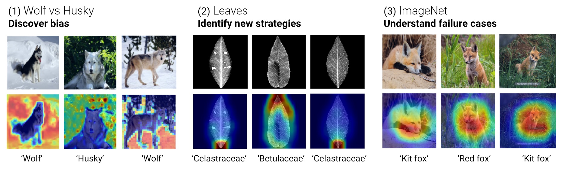
Figure 1: We study the practical usefulness of recent explainability methods in three real-world scenarios, each corresponding to different use cases for XAI. The first dataset is Husky vs. Wolf where the goal of the explanations is to help the user to identify a source of bias in a model (classification is based on the background (snow, grass) as opposed to the animal). The second dataset corresponds to a real-world leaf classification problem which is complex for non-experts. The goal of the explanations is to help the end-user identify the strategy discovered by the vision system. Finally, the third dataset is a subset of ImageNet, which consists of a collection of images where half have been misclassified by the system. The goal of the explanations here is to help the end-user understand the failure sources of a high performing model.

2 Related work

Evaluations based on faithfulness measures

Common approaches [28, 9] measure the faithfulness of an explanation through the change in the classification score when the most important pixels are progressively removed. The bigger the drop, the more faithful is the explanation method. To ensure that the drop in score does not come from a change in the distribution of the perturbed images, the ROAR [51] methods include an additional step whereby the image classifier is re-trained between each removal step. Because these methods do not require ground-truth annotations (i.e. object masks or bounding boxes), they are quite popular in computer vision [28, 9, 12, 24, 25, 29] and natural language processing [52, 53, 12].

Nevertheless, faithfulness measures have recently been criticized as they all rely on a baseline for removing important areas, a baseline that will obviously give better scores to methods relying internally on the same baseline [54]. More importantly, they do not consider humans at any time in the evaluation. As a result, it is unclear if the most faithful attribution method is practically useful to humans.

Evaluations based on humans

A second class of approaches consists in evaluating the ability of humans to leverage explanations for different purposes [6, 10, 57, 58, 59, 60, 30, 61, 62, 55, 56]. [6] were the first to evaluate the usefulness of explanations. Their work focused on the use case of bias detection: they trained a classifier on a biased dataset of wolves and huskies and found that the model consistently used the background to classify. They asked participants if they trusted the model before and after seeing the explanation for the model’s predictions, and found that explanations helped detect bias here. We use a similar dataset to reproduce those results, but our evaluation differs greatly from theirs as we do not ask if participants trust the model but instead measure directly if they understand it.

Closest to our work are [62, 61, 55, 63, 64]. [62, 61, 55] design their evaluation around the notion of simulatability [65, 31]. They introduce different experimental procedures to measure if humans can learn from the explanations how to copy the model prediction on unseen data. Some provide the explanations at test time [62, 61]. Similar to us but for tabular data, [55] proposes to hide explanations at test time, this forces the participants to learn the rules driving the model’s decision at training time where the explanations are shown. There are two limitations to their work: (1) they provide ground-truth labels associated with input images during training, (2) the participants see the same set of images without explanations, and then with explanations, always in that order. This creates learning effects that can heavily bias their results. We differ from their work by: (1) removing ground-truth labels from our framework as they serve no purpose and can bias participants, and (2) we have different participants go through the different conditions. This removes any learning effect, and more importantly, new explainability methods can be evaluated independently and still be compared to the previously evaluated methods. A recent study [63] evaluated how AI systems may be able to assist human decisions by asking participants to identify the correct prediction out of four prediction-explanations pairs shown simultaneously. This measure reflects how well explanations help users tell apart correct from incorrect predictions. While the approach was useful to evaluate explanations in this specific scenario, it is not clear how this framework could be used to evaluate explainability methods more generally. Furthermore, when comparing different types of methods, they adapt the complexity of certain explainability methods to ease the task for participants. We argue that the complexity of explanations is an important property of explanations and that abstracting it away from the evaluation lead to unfair comparisons between methods. In contrast, we propose a more general evaluation framework that can be used for any kind of explainability method without the need to adapt them for the evaluation procedure – hence allowing for an unbiased and scalable comparison between methods. Finally, [64] proposes to evaluate if users are able to identify important features biasing the predictions of a model using a synthetic dataset. By controlling the generation process of the dataset, they have access to the ground-truth attributes biasing the classifier, and can measure the accuracy of users at identifying these features. They evaluate if concept-based or counterfactual explanations help users improve over a baseline accuracy when no explanations are provided, and find no explanation tested to be useful. While both works highlights the importance of human evaluation, they differ in: the metrics employed (identifying relevant features for the model vs. meta-prediction), the type of dataset used (synthetic vs. real-world scenarios), and the type of methods evaluated (counterfactual and concept-based methods vs. attribution methods).

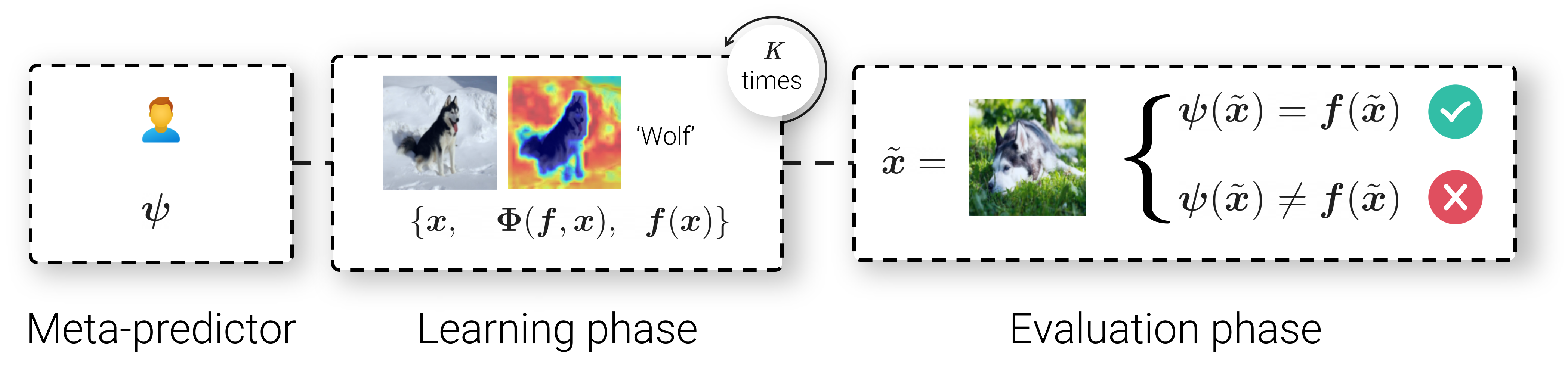
Figure 2: We describe a human-centered framework to evaluate explainability methods borrowing the concept of Meta-predictor. The framework requires a black box model $\bm{f}$ (the predictor), an explanation method $\bm{\Phi}$ and a human subject $\bm{\psi}$ which will try to predict the predictor, hence, the name Meta-predictor. The first step is the learning phase where the Meta-predictor is training using $K$ samples $\bm{x}$, together with the associated model predictions $\bm{f}(\bm{x})$ and explanations $\bm{\Phi}(\bm{f},\bm{x})$. The goal of this learning phase is for the Meta-predictor to uncover the rules driving the decisions of the model from the triplets $(\bm{x},\bm{\Phi}(\bm{f},\bm{x}),\bm{f}(\bm{x}))$. Then, the second step is the evaluation phase where we test the Meta-predictor’s ability to correctly predict the model’s outputs on new samples $\bm{\tilde{x}}$ by comparing its predictions $\bm{\psi}(\bm{\tilde{x}})$ to those of $\bm{f}(\bm{\tilde{x}})$. The Utility score of the explanation method is then computed as the relative accuracy improvement of Meta-predictor trained with vs. without explanations.

3 Proposed evaluation framework

Before providing a rigorous definition of interpretability, let us motivate our approach with an example: a linear classifier is often considered to be readily interpretable because its inner working is sufficiently intuitive that it can be comprehended by a human user. A user can in turn build a mental model of the classifier – predicting the classifier’s output for arbitrary inputs. In essence, we suggest that the model is interpretable because the output can be predicted – i.e, we say we understand the rules used by a model, if we can use those inferred rules to correctly predict its output. This concept of predicting the classifier’s output is central to our approach and we conceptualize the human user as a Meta-predictor of the machine learning model. This notion of Meta-predictor is also closely related to the notion of simulatability [31, 55, 66, 65, 24]. We will now define the term more formally.

We consider a standard supervised learning setting where $\bm{f}$ is a black-box predictor that maps an input $\bm{x}\in\mathcal{X}$ (e.g., an image) to an output $\bm{f}(\bm{x})\in\mathcal{Y}$ (e.g., a class label). One of the main goals of eXplainable AI is to yield useful rules to understand the inner-working of a model $\bm{f}$ such that it is possible to infer its behavior on unseen data points. To correctly infer those rules, the usual approach consists in studying explanations (from Attribution Map, Concept Activation Vectors, Feature Visualization, etc..) for several predictions. Formally, $\bm{\Phi}$ is any explanation functional which, given a predictor $\bm{f}$ and a point $\bm{x}$, provides an information $\bm{\Phi}(\bm{f},\bm{x})$ about the prediction of the predictor. In our experiments, $\bm{\Phi}$ is an attribution method but we would like to remind that the framework is naturally adaptable to other explainability methods such as concept-based methods or feature visualization.

The understandability-completeness trade-off

Different attribution methods will typically produce different heatmaps – potentially highlighting different image regions and/or presenting the same information in a different format. The quality of an explanation can thus be affected by two factors: faithfulness of the explanation (i.e., how many pixels or input dimensions deemed important effectively drive the classifier’s prediction) and the understandability of the explanation for an end-user (i.e., how much of the pattern highlighted by the explanation is grasped by the user).

At one extreme, an explanation can be entirely faithful and provide all the information necessary to predict how a classifier will assign a class label to an arbitrary image (i.e., by giving all the parameters of the classifiers). However, such information will obviously be too complex to be understood by a user and hence it is not understandable. Conversely, an explanation that overly simplifies the model might offer an approximation of the rule used by the model that will be more easily grasped by the user –a more understandable explanation– but this approximation might ultimately mislead the user if it is not faithful. That is to say, just because a human agrees with the evidence pointed out by an explanation does not necessarily mean that it reflects how the model works.

Overall, this means that there is a trade-off between the amount of information provided by an explanation and its comprehensibility to humans. The most useful explanations should lie somewhere in the middle of this trade-off.

The usefulness metric

We describe a new human-centered measure that incorporates this trade-off into a single usefulness measure by empirically evaluating the ability of human participants to learn to “predict the predictor”, i.e., to be an accurate Meta-predictor. Indeed, if an explanation allows users to infer precise rules for the functioning of the predictor on past data, the correct application of these same rules should allow the user to correctly anticipate the model’s decisions on future data. Scrutable but inaccurate explanations will result in an inaccurate Meta-predictor  – just like accurate inscrutable ones. This Meta-predictor framework avoids current pitfalls such as confirmation bias - just because a user likes the explanation does not mean they will be a better Meta-predictor - or prediction leakage on the explanation - in simulatability experiments, as the explanation is available during the test phase, any explanation that leaks the prediction would have a perfect score, without giving us any additional information about the model. We will now formally describe the metric build using this framework.

We assume a dataset $\mathcal{D}=\{(\bm{x}_{i},\bm{f}(\bm{x}_{i}),\bm{\Phi}(\bm{f},\bm{x}_{i})\}_{i=1}^{K}$ used to train human participants to learn to predict a classifier’s output $\bm{f}$ from $K$ samples made of an input image $\bm{x}_{i}$, the associated predictions $\bm{f}(\bm{x}_{i})$ and explanations $\bm{\Phi}(\bm{f},\bm{x}_{i})$. We denote $\bm{\psi}^{(K)}$ a human Meta-predictor after being trained on the dataset $\mathcal{D}$ (see Fig. 2) using explanations. In addition, let $\bm{\psi}^{(0)}$ be the human Meta-predictor after participants were trained on the same dataset but without explanations to offer baseline accuracy scores. We can now define the usefulness of an explainability method $\bm{\Phi}$ after training participants on $K$ samples through the accuracy score of the Meta-predictor normalized by the baseline Meta-predictor accuracy:

$$\textit{Utility-$K$}=\frac{\mathbb{P}(\bm{\psi}^{(K)}(\bm{x})=\bm{f}(\bm{x}))}{\mathbb{P}(\bm{\psi}^{(0)}(\bm{x})=\bm{f}(\bm{x}))}$$ (1)

with $\mathbb{P}(\cdot)$ the probability over a test set. Thus, Utility-$K$ score measures the improvement in accuracy that the explanation has brought. It is important to emphasize that this Utility measure only depends on the classifier prediction and not on the ground-truth label as recommended by [67]. After fixing the number of training samples $K$, we compare the normalized accuracy of different Meta-predictors. The Meta-predictor with the highest score is then the one whose explanations were the most useful as measures compared to a no-explanation baseline.

Utility metric

In practice, we propose to vary the number of observations $K\in\{K_{0},...,K_{n}\}$ and to report an aggregated Utility score by computing the area under the curve (AUC) of the Utility-$K$. The higher the AUC the better the corresponding explanation method is. Formally, given a curve represented by a set of $n$ points $\mathcal{C}=\{(K_{0},\textit{Utility-$K$}_{0}),...,(K_{n},\textit{Utility-$K$}_{n})\}$ where $K_{i-1}<K_{i}$ we define the metric as $\textit{Utility}=AUC(\mathcal{C})$.

4 Experimental design

We first describe how participants were enrolled in the study, then our general experimental design (See SI for more informations).

Participants

Behavioral data were gathered from $n=1,150$ participants using Amazon Mechanical Turk (AMT) (www.mturk.com). All participants provided informed consent electronically and were compensated $\$1.4$ for their time ($\sim 5-8$ min). The protocol was approved by the University IRB and was carried out in accordance with the provisions of the World Medical Association Declaration of Helsinki. For each of the three tested datasets, we ensured that there was a sufficient number of participants after filtering out uncooperative participants ($n=240$ participants, 30 per condition, 8 conditions) to guarantee sufficient statistical power (See SI for details). Overall, the cost of evaluating one method using our benchmark is relatively modest ($50 per test scenario).

General study design

It included 3 conditions: an experimental condition where an explanation is provided to human participants during their training phase (see Fig. 2), a baseline condition where no explanation was provided to the human participants, and a control condition where a bottom-up saliency map [68] was provided as a non-informative explanation. This last control is critical, and indeed lacking from previous work [55, 6], because it provides a control for the possibility that providing explanations along with training images simply increases participants’ engagement in the task. As we will show in Sec. 5, such non-informative explanations actually led to a decrease in participants’ ability to predict the classifier’s decisions – suggesting that giving a wrong explanation is worse than giving no explanations at all.

Each participant was only tested on a single condition to avoid possible experimental confounds. The main experiment was divided into 3 training sessions (with 5 training samples in each) each followed by a brief test. In each individual trial, an image was presented with the associated prediction of the model, either alone for the baseline condition or together with an explanation for the experimental and control condition. After a brief training phase (5 samples), participants’ ability to predict the classifier’s output was evaluated on 7 new samples during a test phase. During the test phase, no explanation was provided to limit confounding effects: one possible effect is if the explanation leaks information about the class label. We also propose to use a reservoir that subjects can refer to during the testing phase to minimize memory load as a confounding factor which was reported in [55] (see SI for an illustration).

Datasets and models

We performed three distinct experiments in total – using a variety of neural network architectures and $6$ representative attributions methods. Each of these experiments aimed at testing the usefulness of the explanation in a different context.

Method	Husky vs. Wolf				Leaves				ImageNet
Session n∘	1	2	3	Utility	1	2	3	Utility	1	2	3	Utility
Baseline	55.7	66.2	62.9		70.1	76.8	78.6		58.8	62.2	58.8
Control	53.3	61.0	61.4	0.95	72.0	78.0	80.2	1.02	60.7	59.2	48.5	0.94
Saliency [17]	53.9	69.6	73.3	1.06	83.2	88.7	82.4	1.13	61.7	60.2	58.2	1.00
Integ.-Grad. [7]	67.4	72.8	73.2	1.15	82.5	82.5	85.3	1.11	59.4	58.3	58.3	0.98
SmoothGrad [8]	68.7	75.3	78.0	1.20	83.0	85.7	86.3	1.13	50.3	55.0	61.4	0.93
GradCAM [10]	77.6	85.7	84.1	1.34	81.9	83.5	82.4	1.10	54.4	52.5	54.1	0.90
Occlusion [18]	71.0	75.7	78.1	1.22	78.8	86.1	82.9	1.10	51.0	60.2	55.1	0.92
Grad.-Input [69]	65.8	63.3	67.9	1.06	76.5	82.9	79.5	1.05	50.0	57.6	62.6	0.95

Table 1: Utility-$K$ and Utility scores. Utility-$K$scores across the 3 sessions for each attribution method, for each of the 3 datasets considered, followed by the Utility scores. Higher is better. The Utility scores of attribution methods that are statistically significant are bolded.

Our first scenario focuses on the detection of biases in AI systems using the popular Wolf vs. Husky dataset from [6] where an evaluation measure was already proposed around the usefulness of explanations for humans to detect biases. This makes it a good control experiment to measure the effectiveness of the framework proposed in Sec. 3. For this first experiment, we used the same model as in the original paper: InceptionV1 [70], and a similar dataset of Husky and Wolf images to bias the model. In this situation where prior knowledge of subjects can affect their Meta-predictor score, we balance data correctness ($50\%$ of correct/incorrect examples shown). Therefore, a subject relying only on their prior knowledge will end up as a bad Meta-predictor of the model. For this experiment, the results come from $n=242$ subjects who all passed our screening process.

In our second scenario, we focus on a representative challenging image categorization task which would be hard to solve by a non-expert untrained human participant and the goal is for the end-user to understand the strategy that was discovered by the AI system. Here, we chose the leaf dataset described in [48]. We selected 2 classes from this dataset (Betulaceae and Celastracea) that could not be classified by shape to reduce the chances that participants will discover the solution on their own – forcing them instead to rely on non-trivial features highlighted by the explanations (veins, leaf margin, etc). This scenario is far from being artificial as it reflects a genuine problem for the paleobotanist [49]. Can explainability methods help non-specialists discover the strategies discovered by an AI system? As participants are lay people from Amazon Mechanical Turk we do not expect them to be experts in botany, therefore we did not explicitly try to control for prior knowledge. In this experiment, $n=240$ subjects passed all our screening and other filtering processes.

Finally, our last scenario focuses on identifying cases where an AI system fails using ImageNet [50], also used in previous explainability work [24, 71, 51, 12, 61, 30]. We used this dataset because we expect it to be representative of real-world scenarios where it is difficult to understand what the model relies on for classification which makes it very difficult to understand these failure cases. Moreover, previous work has pointed out that attribution methods are not useful on this dataset  [61], we have thus chosen to extend our analysis to this particular case. We use a ResNet50 [72] pretrained on this dataset as predictor. Because prior knowledge is a major confounding factor on ImageNet, we select a pair of classes that was heavily miss-classified by the model, to be able to show subjects 50% of correct/incorrect predictions: the pair Kit Fox and Red Fox fits this requirement. In this experiment, we analyzed data from $n=241$ participants who passed our screening and filtering processes.

For all experiments, we compared $6$ representative attribution methods: Saliency (SA) [17], Gradient $\odot$ Input (GI) [19], Integrated Gradients (IG) [7], Occlusion (OC) [18], SmoothGrad (SG) [8] and Grad-CAM (GC) [10]. Further information on these methods can be found in SI. Table 1 summarizes all the results from our psychophysics experiments.

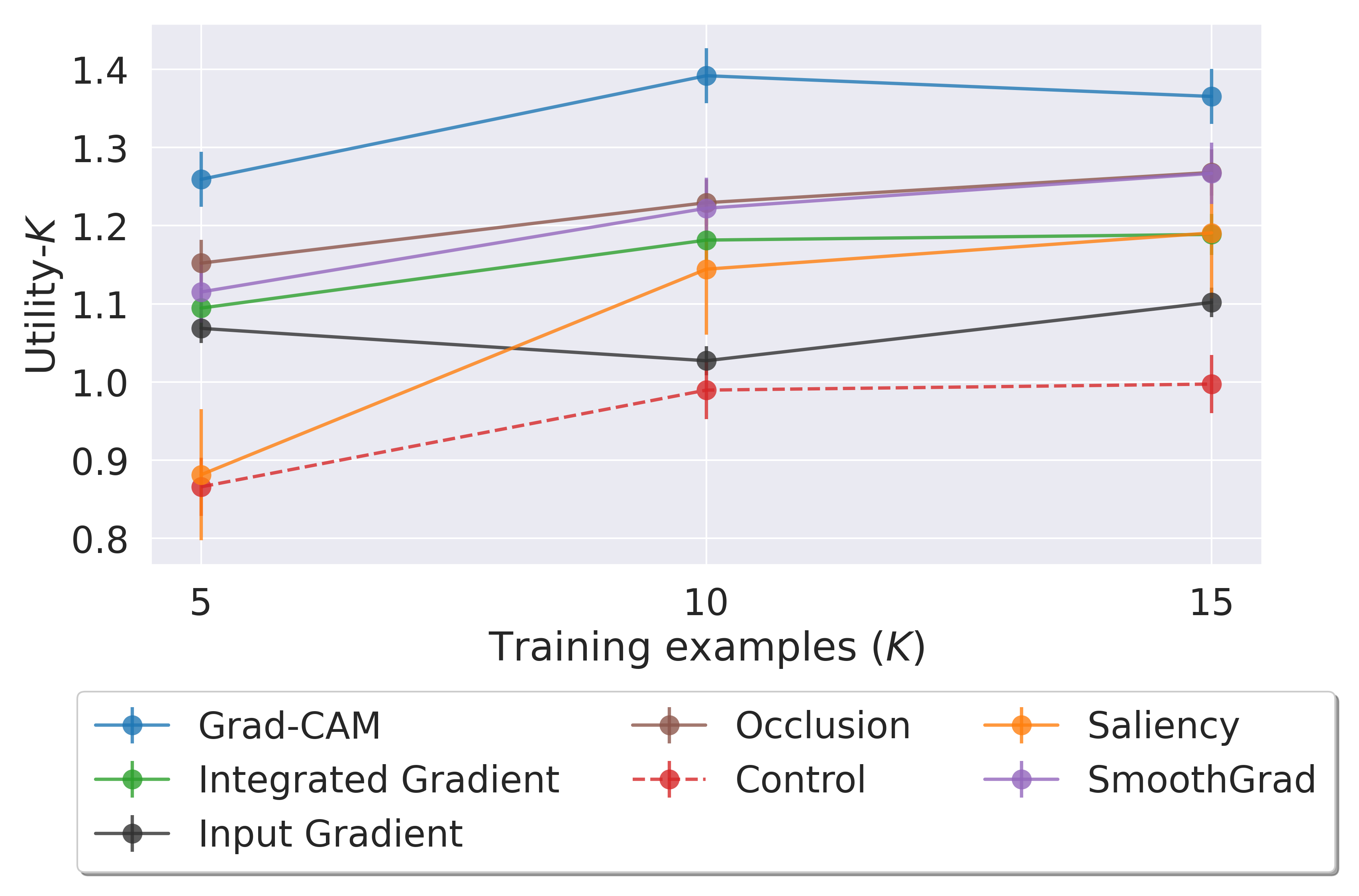
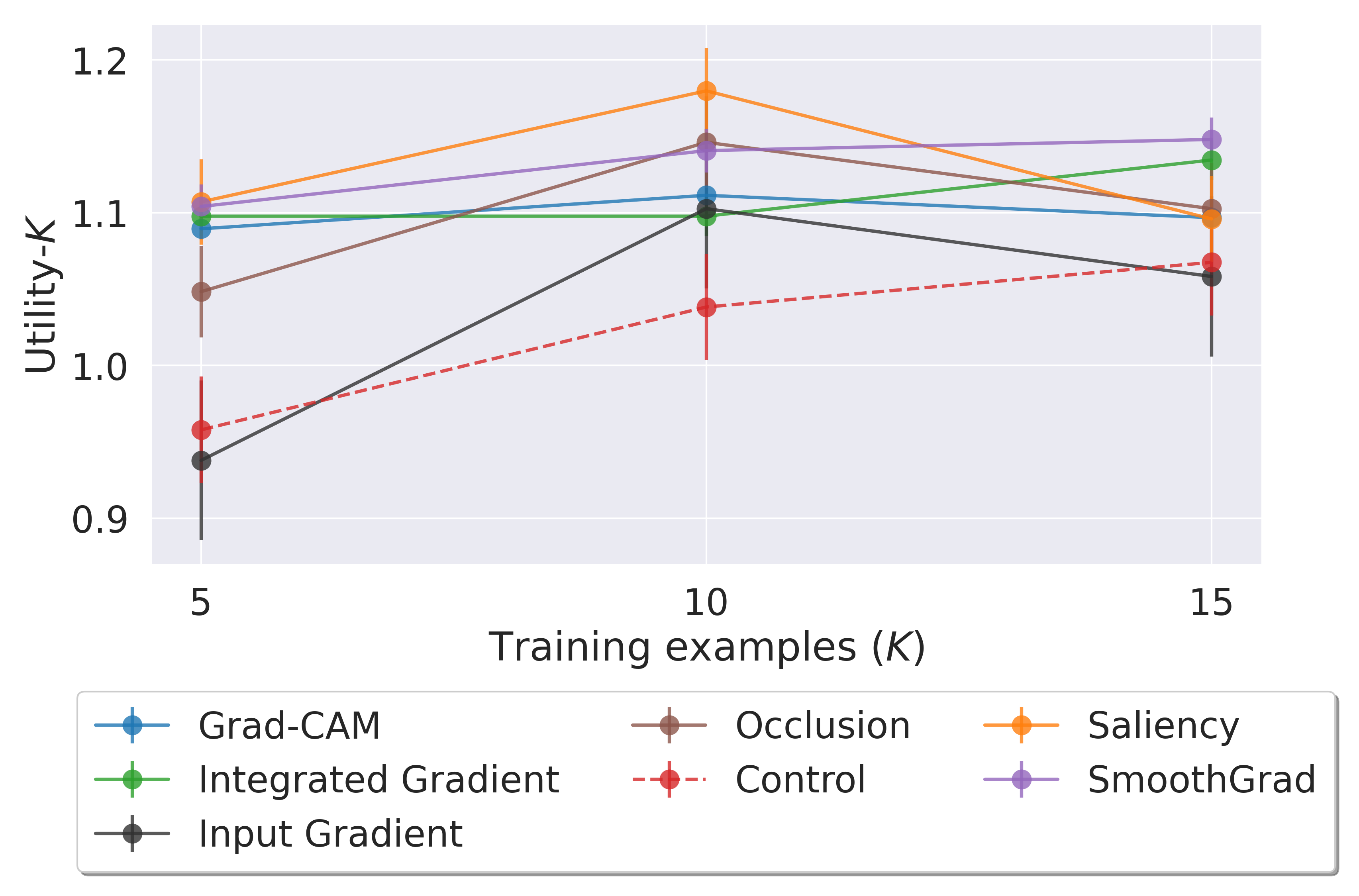
Figure 3: Utility-$K$ for both Husky vs. Wolf (left) and the Leaves (right) dataset. The Utility-$K$ of the explanation, or the accuracy of the human Meta-predictor after training, is measured after each training session (3 in total) for the scenario (1) of bias detection (on the left) and the scenario (2) concerning the identification of new strategies. Concerning the first scenario, all methods have a positive effect on the score obtained - they improve the subjects’ ability to predict the model - and are thus useful to better understand the model. Grad-CAM, Occlusion and SmoothGrad are particularly useful for bias detection. On the Leaves dataset [48], explanations are also useful, but specifically Saliency, SmoothGrad and Integrated Gradients.

5 Results

Scenario (1): Bias detection

Fig. 3 shows the Utility-$K$ scores for each method after different numbers of training samples were used to train participants for the biased dataset of Husky vs. Wolf. The Utility score encodes the quality of the explanations provided by a method, the higher the score, the better the method, with the baseline score being 1 (every score is divided by the baseline score corresponding to human accuracy after training without explanations).

A first observation is that the explanations have a positive effect on the Utility-$K$ score: the explanation allows participants to better predict the model’s decision (as the Utility scores are above 1). These results are consistent with those reported in  [6]. This is confirmed with an Analysis of Variance (ANOVA) for which we found a significant main effect, with a medium effect size ($F(7,234)=9.19,\ p<.001,\ \eta^{2}=0.089$). Moreover, the only score below the baseline is that of the control explanation, which do not make use of the model. We further explore our results by performing pairwise comparisons using Tukey’s Honestly Significant Difference [73] to compare the different explanations against the baseline. We found 3 explainability methods to be significantly better than the baseline: Grad-CAM ($p<0.001$), Occlusion ($p=0.01$) and SmoothGrad ($p=0.034$). Thus, participants who received the Grad-CAM,  Occlusion  or  SmoothGrad  explanations performed much better than those who did not receive them.

Scenario (2): Identifying an expert strategy

In Fig. 3, we show results on the Leaves dataset. An ANOVA analysis across all conditions revealed a significant main effect, albeit small ($F(7,232)=4.29,\ p<.001,\ \eta^{2}=0.042$). This implies that explanation also had a positive effect resulting in better Meta-predictor  in this use case. A Tukey’s Honestly Significant Difference test suggests that the best explanations are Saliency , SmoothGrad and Integrated Gradients as they are the only ones to be significantly better than our baseline (WE) ($p=.004$, $p=.007$ and $p=.03$ respectively). An interesting result is that SmoothGrad seems to be consistently useful across both use cases where explanations are indeed practically useful. A more surprising result is that Saliency which was one of the worst explanations for bias detection, is now the best explanation on this use case (We discuss possible reasons in SI).

Scenario (3): Understanding failure cases

Table 1 shows that, on the ImageNet dataset, none of the methods tested exceeded baseline accuracy. Indeed, the experiment carried out, even with an improved experimental design, led us to the same conclusion as previous works [61]: none of the tested attribution methods are useful (ANOVA: $F(7,233)=1.26,\ p>.05$). In the use case of understanding failure cases on ImageNet, no attributions methods seem to be useful.

Why do attribution methods fail?

After studying the usefulness of attribution methods across 3 real-world scenarios for eXplainable AI, we found that attribution methods help, sometimes, but not always. We are interested in better understanding why sometimes attribution methods fail to help. Because this question has yet to be properly studied, there is no consensus if we can still make attribution methods work on those cases with incremental quantitative improvements. In the follow-up sections we explore 3 hypothesis to answer that question.

Faithfulness as a proxy for Utility?

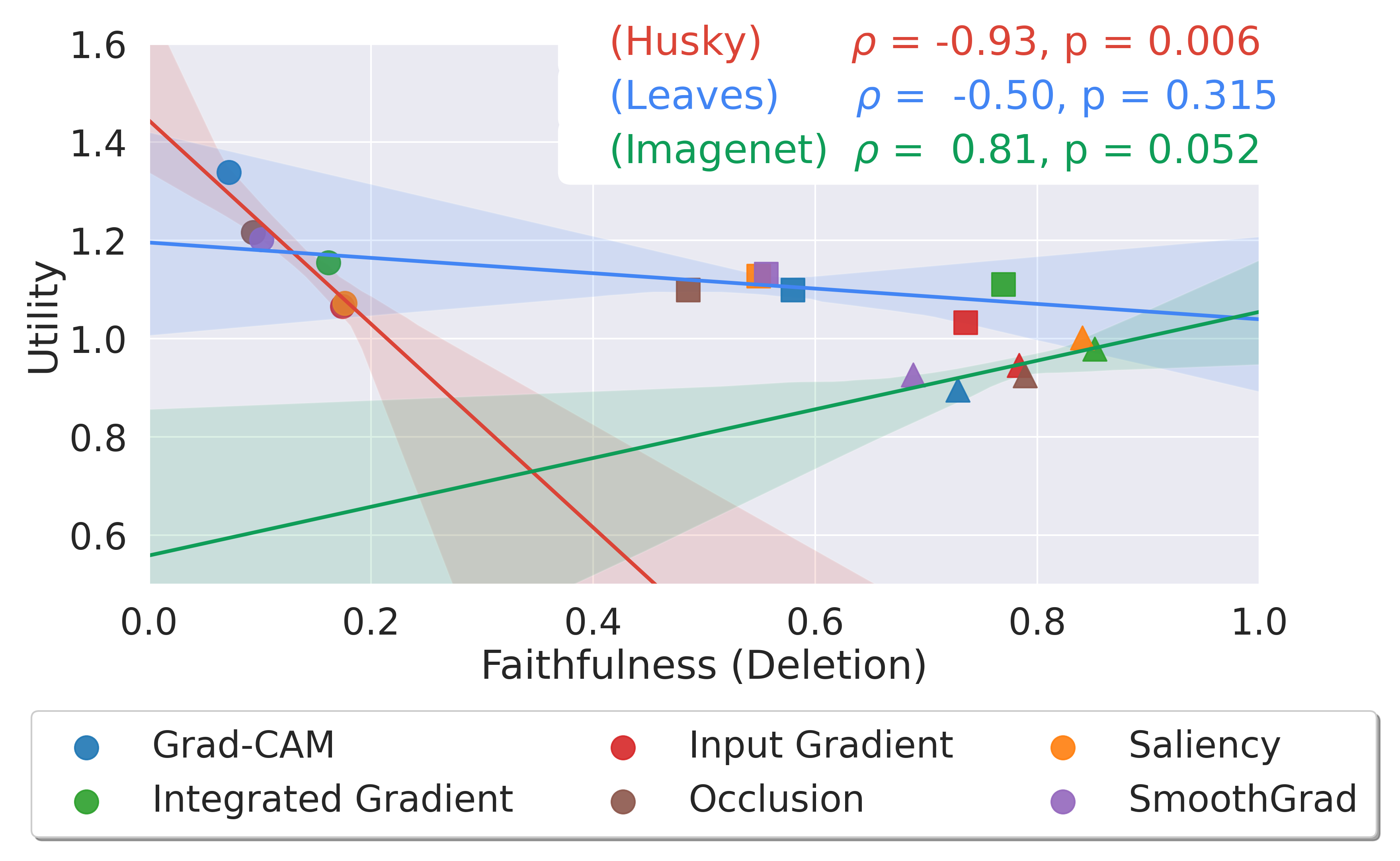
Figure 4: Utility vs Faithfulness correlation. The results suggest that current faithfulness metrics are poor predictors of the end-goal usefulness of explanation methods. Concerning the ImageNet dataset (triangle marker), the Utility scores are insignificant since none of the methods improves the baseline.

Faithfulness is often described as one of the key desiderata for a good explanation [74, 75, 23]. If an explanation fails to be sufficiently faithful, the rules it highlights won’t allow a user to understand the inner-working of the model. Thus, a lack of faithfulness on ImageNet could explain our results. To test this hypothesis, we use the faithfulness metrics: Deletion[28, 9], commonly used to compare attribution methods [28, 9, 12, 24, 25, 29]. A low Deletion score indicates a good faithfulness, thus for ease of reading we report the faithfulness score as $1-$ Deletion such that a higher faithfulness score is better.

Fig 4 shows the linear relationship between our Utility metrics and the faithfulness scores computed for every attribution method across all 3 datasets. We observe two main trends: 1) There does not appear to be any specific pattern regarding faithfulness that could explain why attribution methods are not useful for ImageNet, and 2) the least useful attribution methods for both use cases for which methods help (Bias and Leaves) are some of the leading methods in the field measured by the faithfulness metric. We also found a weak, if maybe anti-correlated, relation between faithfulness and usefulness: just focusing on making attribution methods more faithful does not translate to having methods with higher practical usefulness for end-users. And, in fact, focusing too heavily on faithfulness seem to come at the expense of usefulness, resulting in explanations that are counter-intuitively less useful. This second observation may seems rather alarming for the field given that the faithfulness measure is one of the driving benchmarks.

Are explanations too complex?

Using the trade-off between completeness and understandability previously discussed in Section 3, we formulate another hypothesis: some explanations may be faithful but too complex and therefore cannot be understood by humans. In that view, an explanation with low complexity would tend to be more useful.

As a simple measure of the complexity of visual explanations, it would be ideal to be able to compute the Kolmogorov complexity [76] of each explanation. It was shown in previous work [77] to correlate well with human-derived ratings for the complexity of natural images [78, 79]. As suggested by [76, 80] we used a standard compression technique (JPEG) to approximate the Kolmogorov complexity. Fig. 5 shows the Utility vs complexity score of attribution methods for each dataset. For one of the datasets where attribution methods help, the results suggest the presence of a strong correlation between usefulness and complexity: the least complex method is the most useful to end-users. For the other datasets, the results are either not conclusive (Leaves), or are not relevant as methods are not useful (ImageNet).

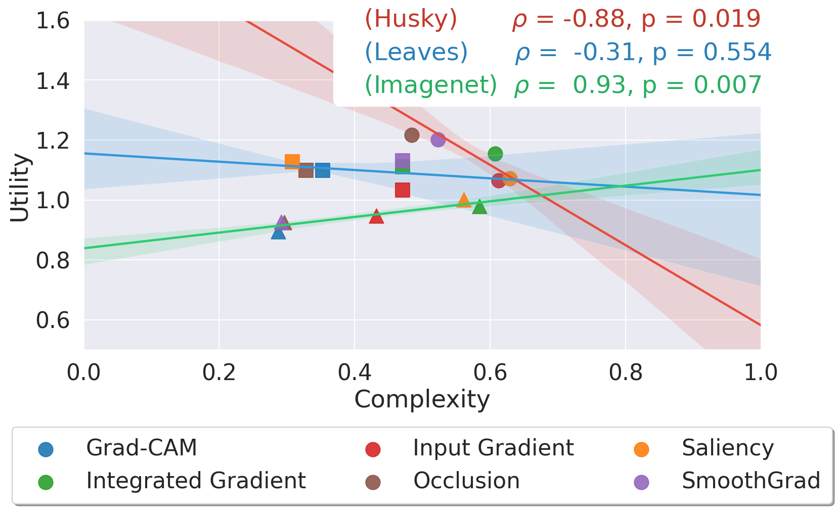
Figure 5: Utility vs Complexity correlation. This suggest a weak but possibly existing link between Complexity  and Utility  scores.

Overall, across datasets there is no significant difference in the complexity of explanations that can explain why attribution methods do not help on ImageNet. This could be because the Kolmogorov Complexity does not perfectly reflect human visual complexity, or because this is not the key element to explain failure cases of attribution methods.

An intrinsic limitation of Attribution methods?

The role of attribution methods is to help identify “where” to look in an image to understand the basis for a system’s prediction. However, attribution methods do not tell us “what” in those image regions is driving decisions. For categorization problems which involve perceptually similar classes (such as when discriminating between different breeds of dogs) and fine-grained categorization problems more generally, simply looking at diagnostic image regions tells the user very little about the specific shape property being relevant. For instance, knowing that the ear shape is being used for recognition does not say what specific shape feature is being encoded (e.g., pointed vs. round or narrow vs. broad base, etc). Our main hypothesis is that such a lack of explicit “what” information is precisely what is driving the failure of attribution methods on our ImageNet use-case.

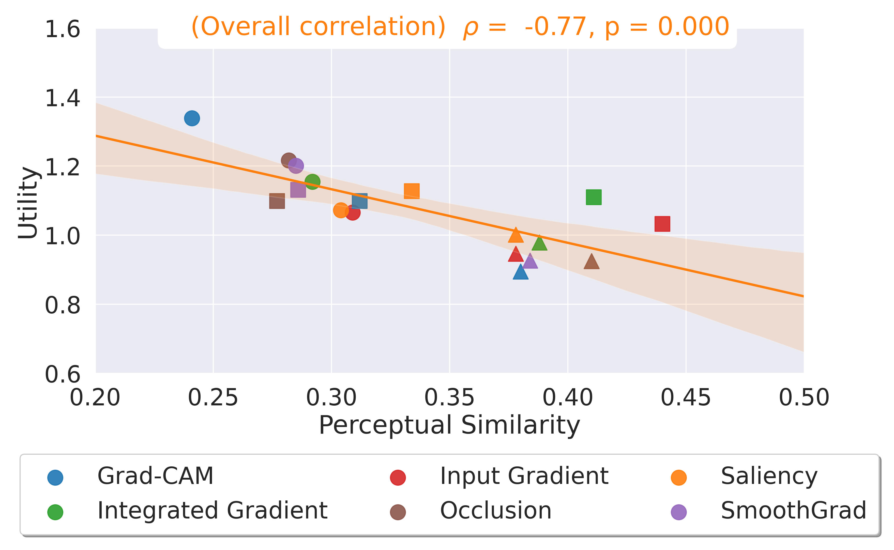
Figure 6: Perceptual Similarity scores vs. Utility. The perceptual similarity of highlighted regions by a given attribution method for both classes is measured, for each method, for each dataset. We observe a strong correlation between the perceptual similarity of features highlighted for both classes and the practical usefulness of methods.

To test this hypothesis, we estimated the perceptual similarity between classes measured within diagnostic regions (see SI for more details) using the Learned Perceptual Image Patch Similarity (LPIPS) metric [81] as it has been shown to approximate human perceptual similarity judgments well [81, 82]. We report the perceptual similarity score as 1 - LPIPS score so that a high score means a high similarity. Fig. 6 shows the correlation between the perceptual similarity scores vs. our Utility scores on all methods and datasets studied. Our results suggest a strong correlation between perceptual similarity and practical usefulness: the more perceptually similar discriminative features of both classes are, the less useful attribution methods become. More importantly, the results across datasets show that on ImageNet, where attribution methods do not help, every method has a high similarity score. This result suggests that after a certain threshold of perceptual similarity, attribution methods might no longer be useful, no matter how faithful or low in complexity the explanation is. Overall, the results suggest that the perceptual similarity of discriminative features could explain why attribution methods fail on ImageNet.

6 Discussion

In summary, we conducted a large-scale human psychophysics experiment to test the utility of explainability methods in real-world scenarios. Our work shows that in two of the three tested scenarios (bias detection and identification of new strategies), explainability methods have indeed progressed and they provide meaningful assistance to human end-users. Nevertheless, we identified a scenario (understanding failure case) for which none of the tested attribution methods were helpful. This result is consistent with previous work [61] and highlights a fundamental challenge for XAI.

Further analysis of associated faithfulness performance metrics driving the development of explainability methods revealed that they did not correlate with our empirical measure of utility – suggesting that they might not be suited anymore to move the field forward. We also investigated the possibility that the complexity of individual explanations may play a role in explaining human failures to learn to leverage those explanations to understand the model and, while we found a weak correlation between complexity and our empirical measure of utility, this correlation appears too low to explain the failure of these methods.

Finally, because attribution methods appear to be just as faithful and low in complexity whether they are useful or not, we explored the possibility that their failure lies, not in the quality of their explanations, but in the intrinsic limitations of attribution methods. If fully grasping the strategy of a model requires understanding, not just “where” to look (as revealed by attribution maps) but also “what” to look at, something not currently revealed by these methods, attribution methods will not help. Our assumption is that the need for finer “what” information should arise when diagnostic image locations across classes look perceptually very similar and potentially semantically related for certain classification problems (e.g., looking at the ears or the snout to discriminate between breeds of cats and dogs) and one needs to identify what visual features are driving decisions. We computed a perceptual score for classification problems by estimating the perceptual similarity between diagnostic image regions (as predicted by attribution methods) and found that, indeed, when this score predicts a certain level of perceptual similarity between classes, attribution methods fail to contribute useful information to human users, regardless of the faithfulness or complexity of the explanations. This suggests that explainability methods may need to communicate additional information to the end user beyond attribution maps.

7 Limitation and broader impact

Limitations.

Our definition of the usefulness of an explanation is quite general. However, there are several limitations associated with our approach to estimate usefulness. First, our approach does not take into account the level of machine learning expertise of the user (the most useful explanation for a novice might not be the best one for an expert). Second, the need for human participants to evaluate explanations brings challenges compared with the automated metrics currently used in the field. However, by releasing all our data and software , we hope to encourage the adoption of the approach to evaluate future explainability methods and to assess the overall progress towards the development of more human-interpretable AI systems.

Broader impacts.

While the increasing use of AI in real-world scenarios has shown potential to do good [46, 47, 48], it has also shown its potential for harm, especially when models rely on shortcuts (e.g., relying on spurious correlations in the training set that leads to unintended racial bias [39, 40, 41]). To identify such shortcuts, the field of Explainable AI has developed a lot of explainability methods; but it is not always clear which one performs best when trying to understand a model. We hope our evaluation method can help in this regard, assisting the AI practitioner in better identifying bias and shortcuts that may unfairly discriminate against groups of people.

Appendix A Human experiments

A.1 Experimental design

Figure 7 summarizes the experimental design used for our experiments. The participants that went through our experiments are users from the online platform Amazon Mechanical Turk (AMT). Through this platform, users stay anonymous, hence, we do not collect any sensitive personal information about them. We prioritized users with a Master qualification (which is a qualification attributed by AMT to users who have proven to be of excellent quality) or normal users with high qualifications (number of HIT completed $=10000$ and HIT accepted $>98\%$).

Before going through the experiment, participants are asked to read and agree to a consent form, which specifies: the objective and procedure of the experiment, as well as the time expected to completion ($\sim 5$ - $8$ min) with the reward associated ($\$1.4$), and finally, the risk, benefits, and confidentiality of taking part in this study. There are no anticipated risks and no direct benefits for the participants taking part in this study.

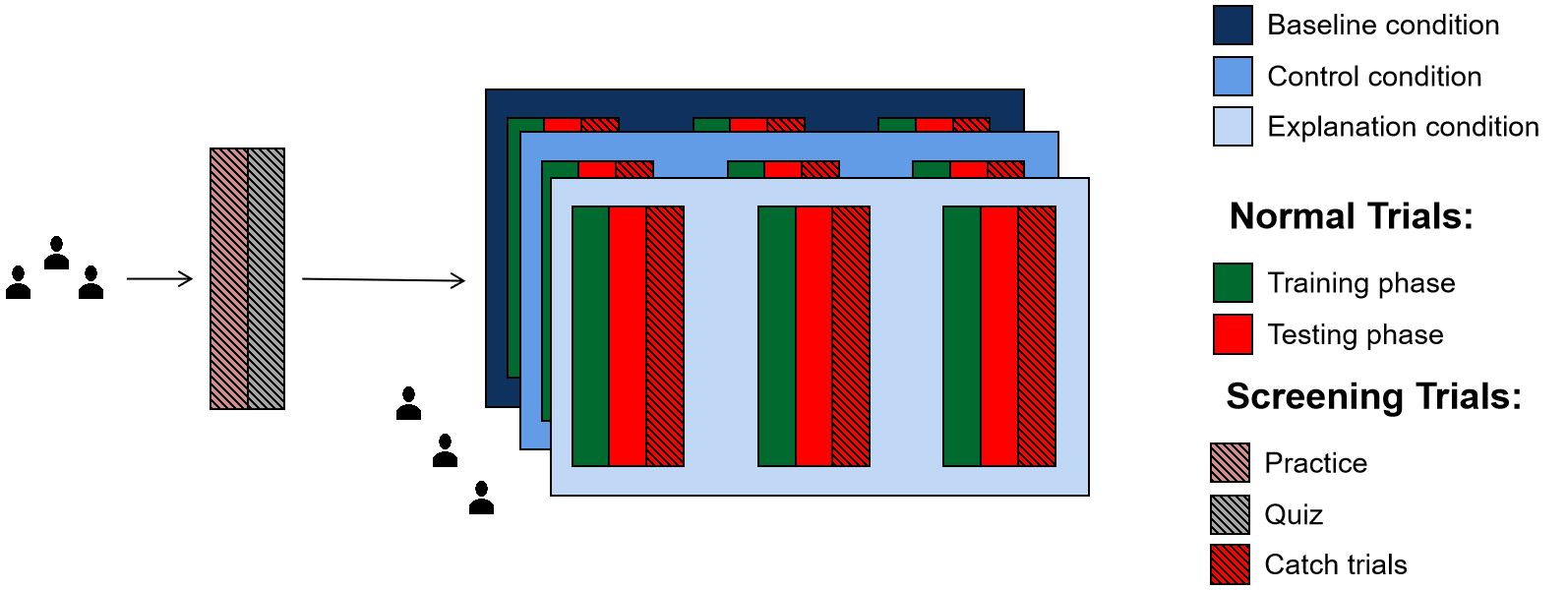
Figure 7: Experimental design. First, every participant goes through a practice session (fig 8) to make sure they understand how to use attribution methods to infer the rules used by a model, and a quiz (fig 9) to make sure they actually read and understand the instructions. Then, participants are split into the different conditions – every participant will only go through one condition. The 3 possible conditions are: an Explanation condition where an explanation is provided to human participants during their training phase, a Baseline condition where no explanation was provided to the human participants, and a Control condition where a non-informative explanation was provided. The main experiment was divided into 3 training sessions each followed by a brief test. In each individual training trial, an image was presented with the associated prediction of the model, either alone for the baseline condition or together with an explanation for the experimental and control condition. After a brief training phase (5 samples), participants’ ability to predict the classifier’s output was evaluated on 7 new samples (only the image, no explanation) during a test phase. To filter out uncooperative participants we also add a catch trial (fig 10) in each test session.

Controlling for prior class knowledge

To control for users’ own semantic knowledge, we balanced the samples shown to participants so that the classifiers were correct/incorrect 50% of the time. This way, the baseline (participants who try to simply predict the true class label of an image as opposed to learning to predict the model’s outputs) is at 50%. Any higher score reflects a certain understanding of the rules used by the model.

A.2 Pruning out uncooperative participants

3-stage screening proccess.

To prune out uncooperative participants, we subjected them to a 3-stage screening process. First, participants completed a short practice session to make sure they understood the task and how to use the attribution methods to infer the rules used by the model (fig 8). Second, as done in [83], we asked participants to answer a few questions regarding the instructions provided to make sure they actually read and understood them (fig 9). Third, during the main experiment, we took advantage of the reservoir to introduce a catch trial (fig 10). The reservoir is the place where we store the training example of the current session, which can be accessed during the testing phase. We added a trial in the testing phase of each session where the input image corresponded to one of the training samples used in the current session: since the answer is still on the screen (or a scroll away) we expect participants to be correct on these catch trials. Participants that failed any of the 3 screening processes were excluded from further analysis.

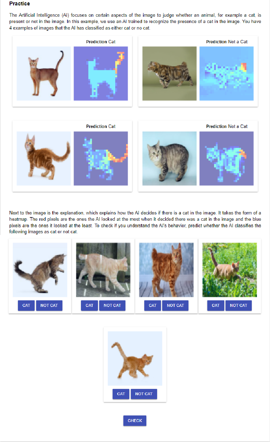
Figure 8: Practice session. Through a practice session, which is a simplified version of the main experiment, we evaluate if users understand how to read and use explanations. Participants that failed to predict correctly any of the 5 cat test images on the first try were excluded from further analysis.

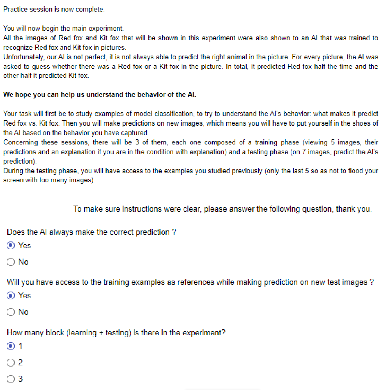
Figure 9: Quiz. Through a quiz, we make sure that users read and understood the instructions. Participants that did not answer correctly every question on the first try were excluded from further analysis.

A.3 More results

Reaction time.

We explored whether the usefulness of a method is reflected in the reaction time of participants -i.e., the more useful the explanation the faster the participants are able to grasp the strategy of the model-. Table 2 shows the reaction time of participants across methods, across datasets. We do not find any trend linking reaction time with usefulness.

Method	Husky vs. Wolf	Leaves	ImageNet
Saliency [17]	207.7	212.9	202.3
Integ.-Grad. [7]	213.1	216.5	218.5
SmoothGrad [8]	215.8	268.8	243.9
GradCAM [10]	168.9	154.6	268.9
Occlusion [18]	221.2	229.2	274.4
Grad.-Input [69]	210.4	238.1	208.0

Table 2: Average total time per method per dataset (in second). For each dataset, we bold the most useful method, and we underline the least useful method.

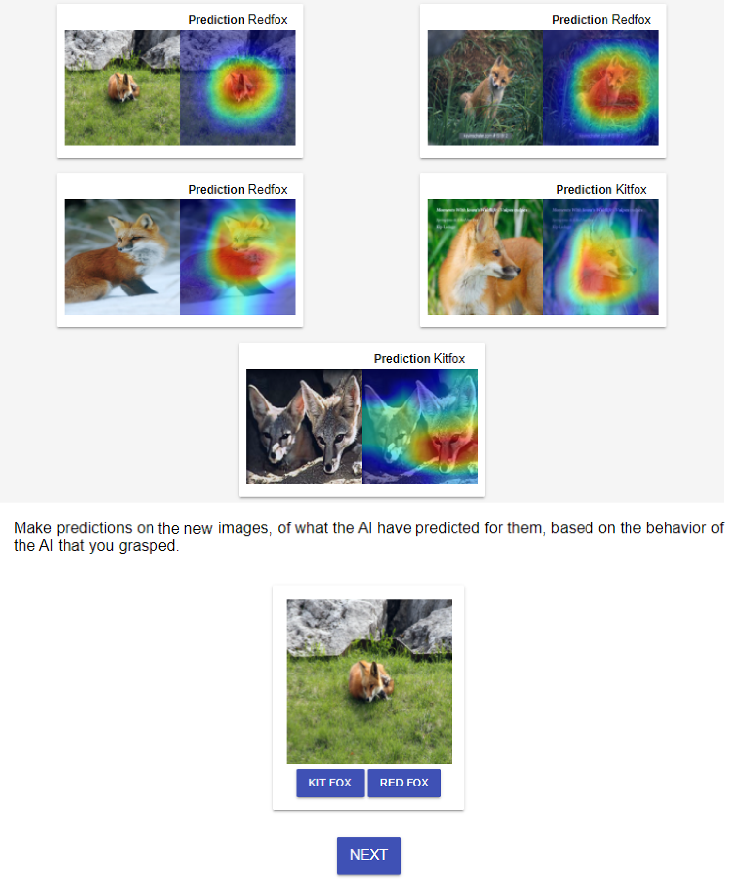
Figure 10: Catch trial. We use a reservoir (to store all the examples of the current training session) that participants can refer to during the testing phase to minimize memory load. At the top of the screen is the reservoir, at the bottom of the screen is a trial from the testing phase. We take advantage of the reservoir to introduce a catch trial. We added a trial in the testing phase of each session where the input image corresponded to one of the training samples used in the current session: since the answer is still on the screen (or a scroll away) we expect participants to be correct on these catch trials. Participants that failed any of the 3 catch trials (one per session) were excluded from further analysis.

Appendix B Why do the best methods for the use cases Bias detection and Identifying an expert strategy (leaves) differ?

The most interesting case is Saliency, which is the worst method on the bias dataset but the best on the “leaves” dataset. On the bias dataset, the model seems to focus on the background (i.e., a coarse feature), and on the “leaves” dataset the model seems to focus either on the margin or on the vein of the leaf (i.e., very fine features). We hypothesize that different methods suit different granularity of features (coarse vs fine). [8] make the hypothesis that “the saliency maps are faithful descriptions of what the network is doing” but because “the derivative of the score function with respect to the input [is] not […] continuously differentiable”, the saliency map can appear noisy. Because of this local discontinuity of the gradient, a large patch of important pixels is often portrayed in the saliency map as a collection of smaller patches of important pixels (i.e., a coarse feature vs multiple individual fine features) which can make it hard to identify if the strategy is the coarse feature or a more complex interaction of the smaller features. In the bias dataset, because the model relies on the background, the Saliency maps appear very noisy and the explanation ends-up not being useful. We note that SmoothGrad, which proposes to fix that discontinuity, is useful. On the other hand, on the leaves dataset, the model uses very fine features, therefore the Saliency maps suffer less from the discontinuity, it does not appear noisy, Saliency is useful. We also note that in this case, SmoothGrad is not better than Saliency, which can arguably be attributed to the fact that we do not need to fix the discontinuity of the gradient. Conversely, because the granularity of both Grad-CAM (the feature map is much smaller than image size) and Occlusion (the patch size is much bigger than a pixel) is too high, the heatmaps they offer on the “leaves” dataset are too coarse to specifically highlight the fine features and it seems to take more time for the subjects to pick-up on them. But on the biased dataset, Grad-CAM and Occlusion are the best performing methods.

Appendix C Why do attribution methods fail?

C.1 Faithfulness

While the Deletion[9] measure is the most commonly used faithfulness metric, for completeness we also consider 2 others faithfulness metric available in the Xplique library[84]: Insertion[9] and $\mu$Fidelity[74]. Fig 11 shows the correlation between either measure and our Utility. We find them to be no better predictor of the practical usefulness of attribution methods than the Deletion measure.

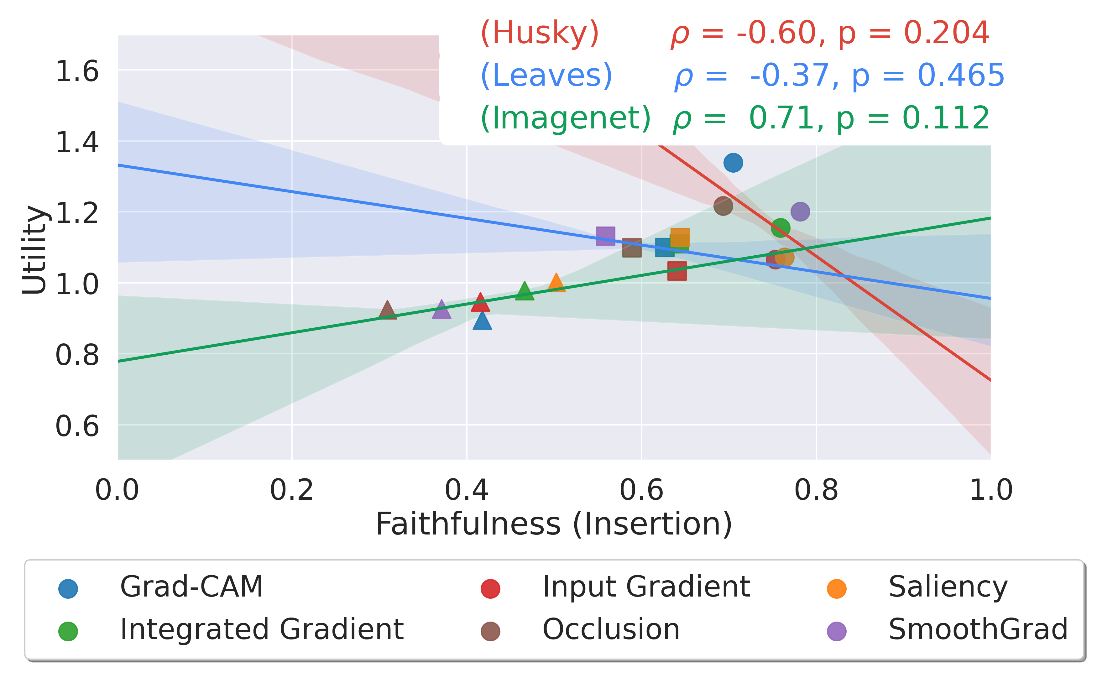
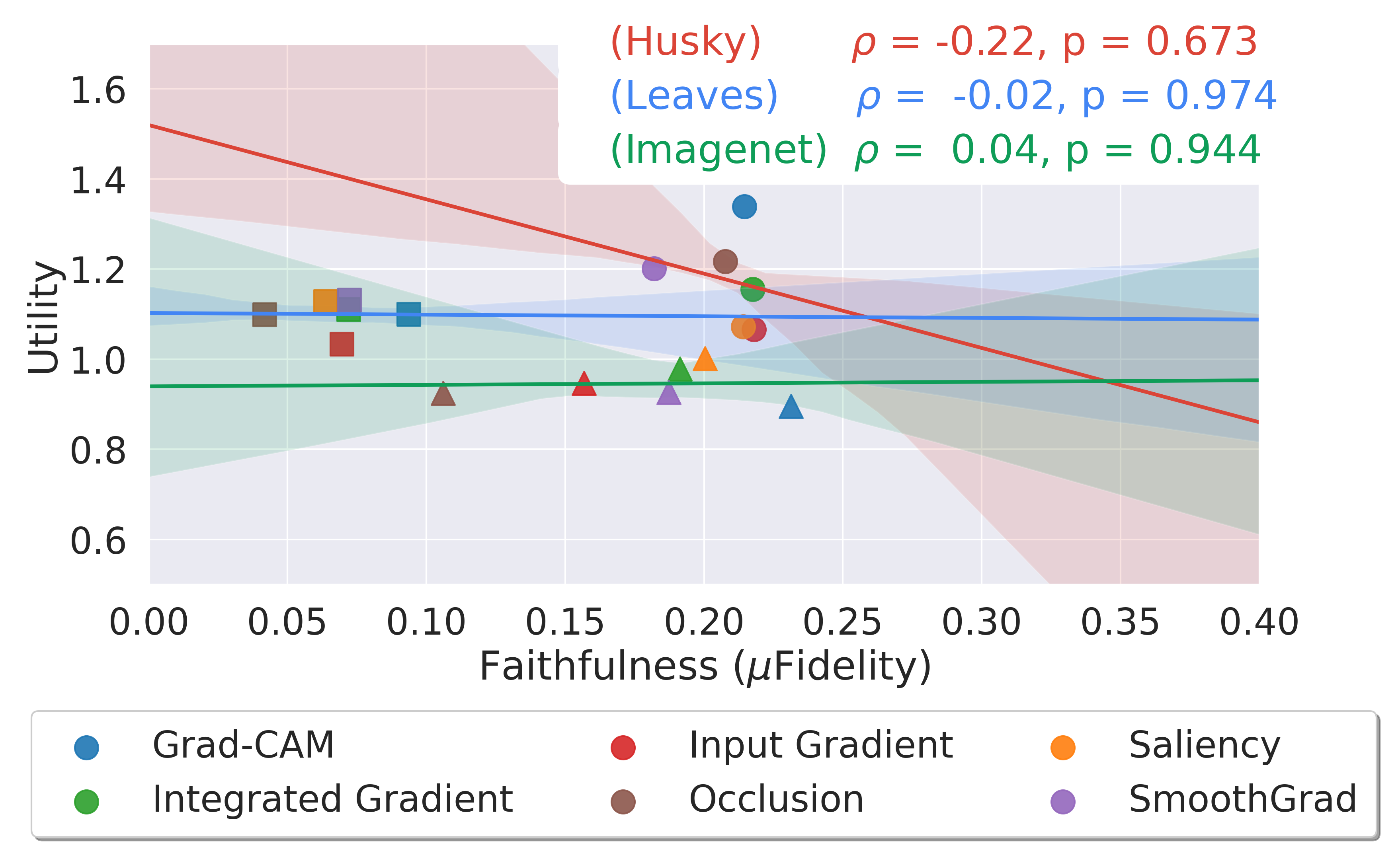
Figure 11: Utility vs Insertion correlation & Utility vs $\mu$Fidelity correlation The results suggest that every faithfulness metrics tested are poor predictors of the practical usefulness of attribution methods. Concerning the ImageNet dataset (triangle marker), the Utility scores are insignificant since none of the methods improves the baseline.

C.2 Perceptual Similarity

Method	Husky vs. Wolf	Leaves	ImageNet
Saliency [17]	0.304	0.334	0.378
Integ.-Grad. [7]	0.292	0.411	0.388
SmoothGrad [8]	0.285	0.286	0.384
GradCAM [10]	0.241	0.312	0.38
Occlusion [18]	0.282	0.277	0.41
Grad.-Input [69]	0.309	0.44	0.378

Table 3: Perceptual Similarity scores. The perceptual similarity of highlighted regions by a given attribution method for both classes is measured, for each method, for each dataset. The perceptual similarity scores that are higher than $0.378$ (the minimum score on ImageNet) are bolded. Higher is more similar.

Tab 3 shows the Perceptual Similarity scores obtained for each method, on every dataset. We observe that on ImageNet, where attribution methods do not help, the perceptual similarity scores are clearly higher than on the two other datasets, where attribution methods help.
Fig 12 shows examples of patches for each dataset using Grad-CAM.

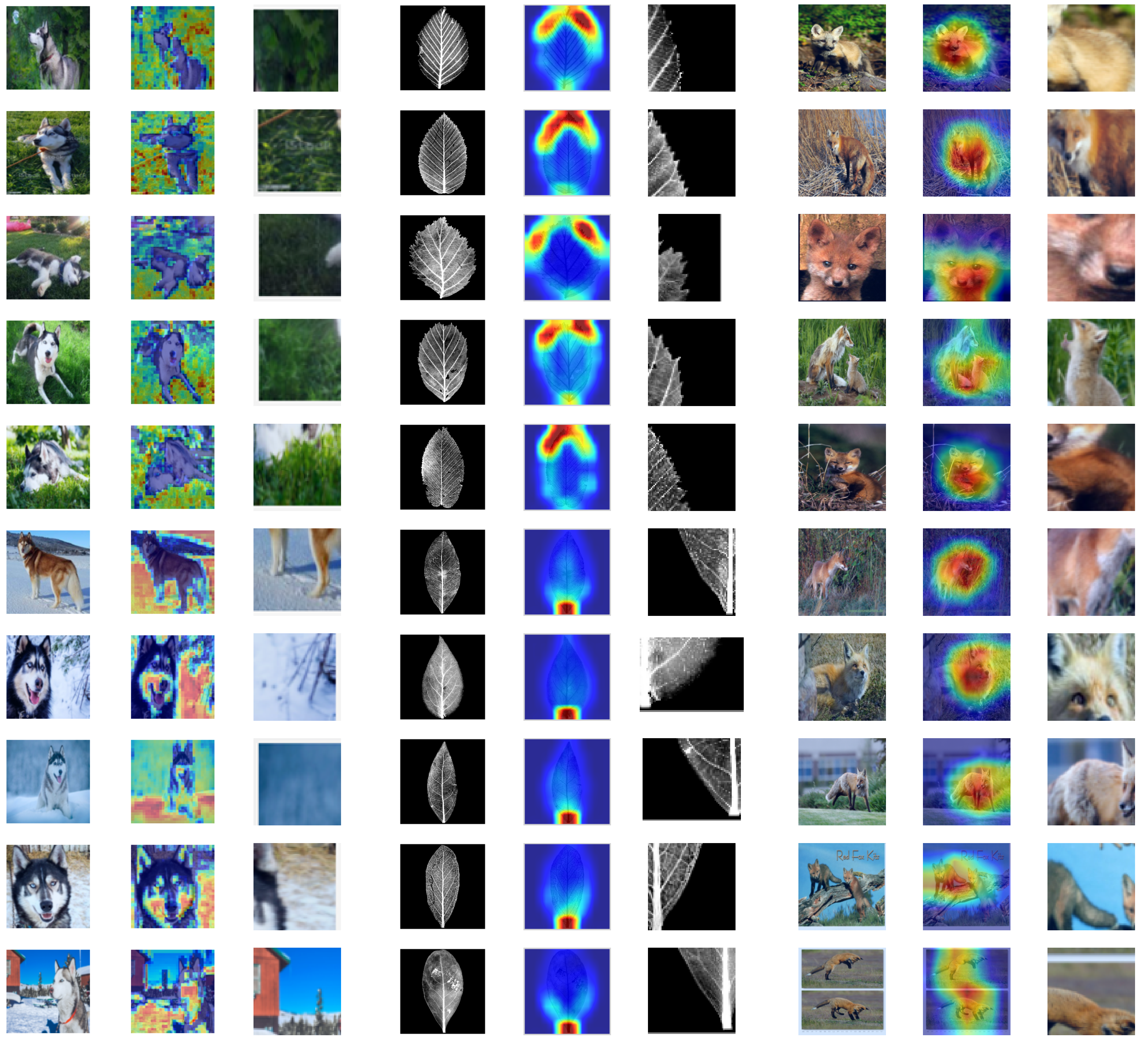
Figure 12: Examples of extracted patches. The perceptual similarity score is performed on the locations considered most important by the attribution methods. Examples of patches extracted for the three datasets with the Grad-CAM  method.

Appendix D Attribution methods

D.1 Methods

In the following section, the formulation of the different methods used in the experiment is given. We define $\bm{f}(\bm{x})$ the logit score (before softmax) for the class of interest. An explanation method provides an attribution score for each input variables. Each value then corresponds to the importance of this feature for the model results.

Saliency [17] is a visualization technique based on the gradient of a class score relative to the input, indicating in an infinitesimal neighborhood, which pixels must be modified to most affect the score of the class of interest.

$$\bm{\Phi}^{SA}(\bm{x})=||\nabla_{\bm{x}}\bm{f}(\bm{x})||$$

Gradient $\odot$ Input [69] is based on the gradient of a class score relative to the input, element-wise with the input, it was introduced to improve the sharpness of the attribution maps. A theoretical analysis conducted by [19] showed that Gradient $\odot$ Input is equivalent to $\epsilon$-LRP and DeepLIFT [85] methods under certain conditions: using a baseline of zero, and with all biases to zero.

$$\bm{\Phi}^{GI}(\bm{x})=\bm{x}\odot||\nabla_{\bm{x}}\bm{f}(\bm{x})||$$

Integrated Gradients [7] consists of summing the gradient values along the path from a baseline state to the current value. The baseline is defined by the user and often chosen to be zero. This integral can be approximated with a set of $m$ points at regular intervals between the baseline and the point of interest. In order to approximate from a finite number of steps, we use a Trapezoidal rule and not a left-Riemann summation, which allows for more accurate results and improved performance (see [86] for a comparison). The final result depends on both the choice of the baseline $\mathbb{x}_{0}$ and the number of points to estimate the integral. In the context of these experiments, we use zero as the baseline and $m=80$.

$$\bm{\Phi}^{IG}(\bm{x})=(\bm{x}-\bm{x}_{0})\int_{0}^{1}\nabla_{\bm{x}}\bm{f}(\bm{x}_{0}+\alpha(\bm{x}-\bm{x}_{0})))d\alpha$$

SmoothGrad [8] is also a gradient-based explanation method, which, as the name suggests, averages the gradient at several points corresponding to small perturbations (drawn i.i.d from a normal distribution of standard deviation $\sigma$) around the point of interest. The smoothing effect induced by the average helps reduce the visual noise and hence improve the explanations. In practice, Smoothgrad is obtained by averaging after sampling $m$ points. In the context of these experiments, we took $m=80$ and $\sigma=0.2$ as suggested in the original paper.

$$\bm{\Phi}^{SG}(\bm{x})=\mathbb{E}_{\varepsilon\sim\mathcal{N}(0,\bm{I}\sigma)}(\nabla_{\bm{x}}\bm{f}(\bm{x}+\varepsilon))$$

Grad-CAM [10] can be used on Convolutional Neural Network (CNN), it uses the gradient and the feature maps $\mathbb{A}^{k}$ of the last convolution layer. More precisely, to obtain the localization map for a class, we need to compute the weights $\alpha_{c}^{k}$ associated to each of the feature map activation $\mathbb{A}^{k}$, with $k$ the number of filters and $Z$ the number of features in each feature map, with $\alpha_{k}^{c}=\frac{1}{Z}\sum_{i}\sum_{j}\frac{\partial{\bm{f}(\bm{x})}}{\partial\mathbb{A}^{k}_{ij}}$ and

$$\bm{\Phi}^{GC}=max(0,\sum_{k}\alpha_{k}^{c}\mathbb{A}^{k})$$

Notice that the size of the explanation depends on the size (width, height) of the last feature map, a bilinear interpolation is performed in order to find the same dimensions as the input.

Occlusion [18] is a sensitivity method that sweeps a patch that occludes pixels over the images, and uses the variations of the model prediction to deduce critical areas. In the context of these experiments, we took a patch size and a patch stride of of 1 tenth of the image size.

$$\bm{\Phi}^{OC}_{i}=\bm{f}(\bm{x})-\bm{f}(\bm{x}_{[\bm{x}_{i}=0]})$$

D.2 Examples of explanations

Examples of explanations from the different attributions methods evaluated through our experiments on the Husky vs. Wolf dataset (fig 13), the Leaves dataset (fig 14) and the ImageNet dataset (fig 15).

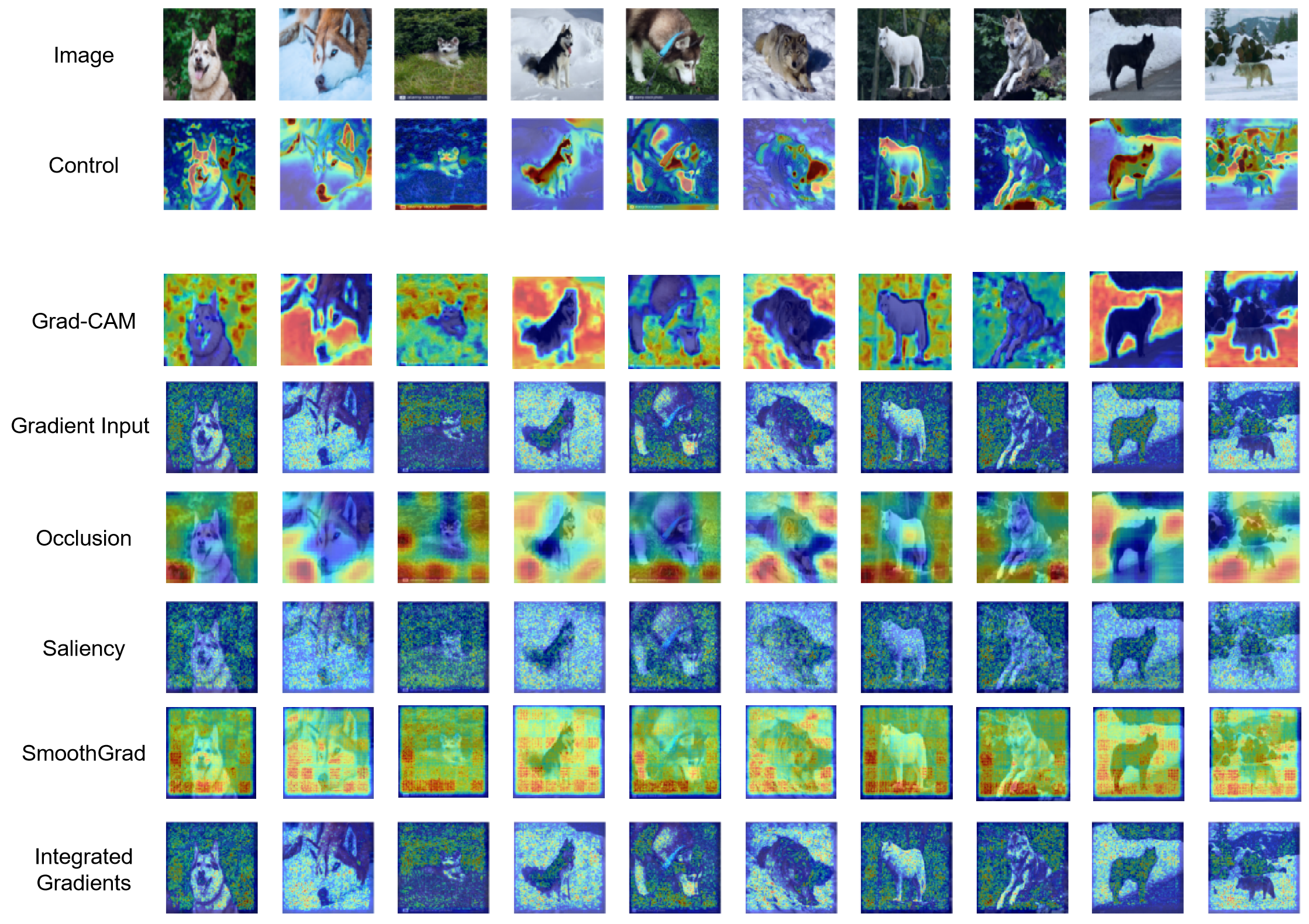
Figure 13: Examples of images from the Wolf vs. Husky experiment, alongside their respective: Control explanation (which is a non-informative explanation) as well as the different Attribution methods evaluated in our experiment.

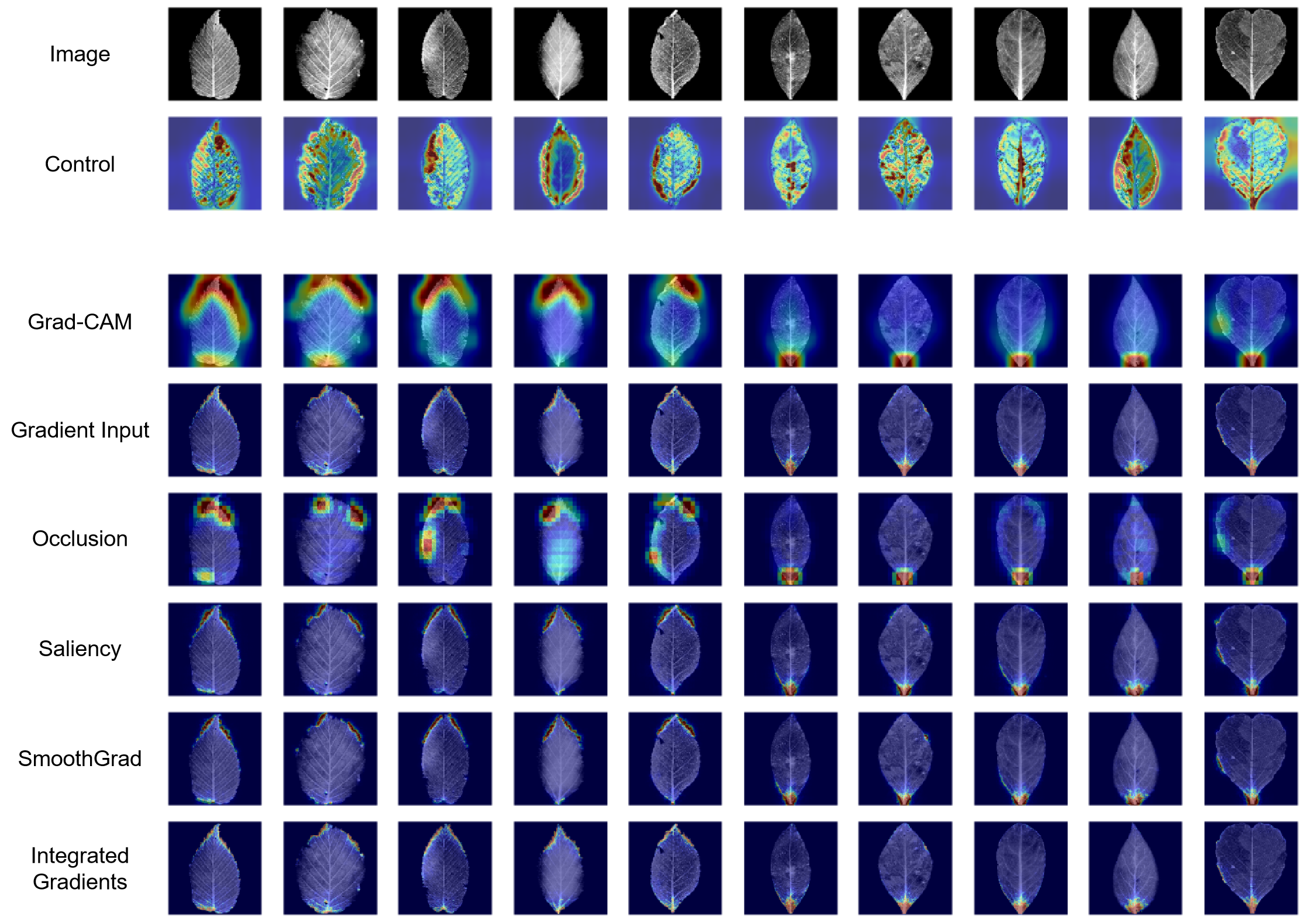
Figure 14: Examples of images from the Leaves experiment, alongside their respective: Control explanation (which is a non-informative explanation) as well as the different Attribution methods evaluated in our experiment.

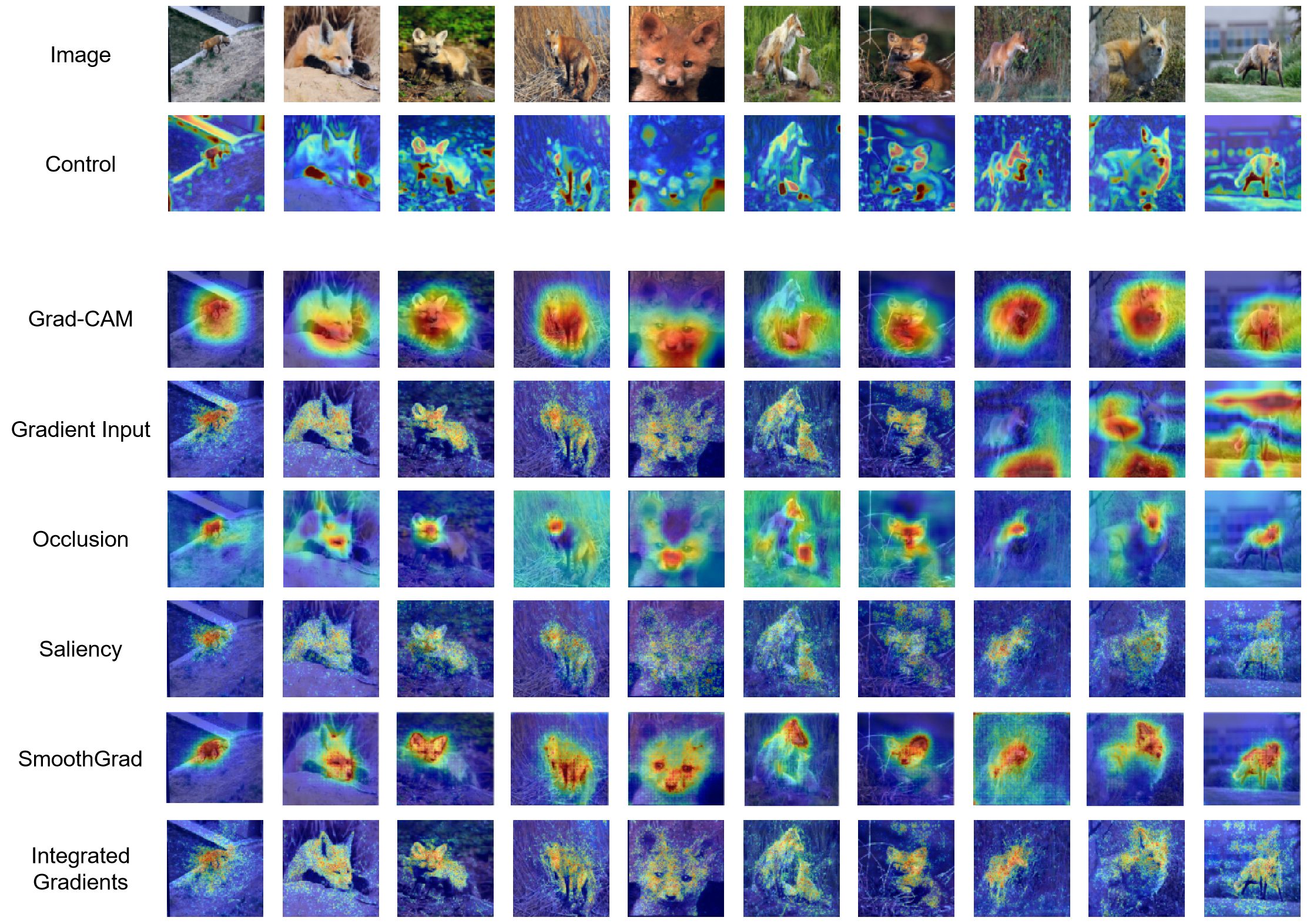
Figure 15: Examples of images from the ImageNet experiment, alongside their respective: Control explanation (which is a non-informative explanation) as well as the different Attribution methods evaluated in our experiment.

Checklist

1. For all authors…

   1. Do the main claims made in the abstract and introduction accurately reflect the paper’s contributions and scope? [Yes]

   2. Did you describe the limitations of your work? [Yes]

   3. Did you discuss any potential negative societal impacts of your work? [No] We identify no potential negative societal impacts.

   4. Have you read the ethics review guidelines and ensured that your paper conforms to them? [Yes]

2. If you are including theoretical results…

   1. Did you state the full set of assumptions of all theoretical results? [Yes]

   2. Did you include complete proofs of all theoretical results? [Yes] In the SI.

3. If you ran experiments…

   1. Did you include the code, data, and instructions needed to reproduce the main experimental results (either in the supplemental material or as a URL)? [Yes] As a URL

   2. Did you specify all the training details (e.g., data splits, hyperparameters, how they were chosen)? [N/A]

   3. Did you report error bars (e.g., with respect to the random seed after running experiments multiple times)? [N/A]

   4. Did you include the total amount of compute and the type of resources used (e.g., type of GPUs, internal cluster, or cloud provider)? [N/A]

4. If you are using existing assets (e.g., code, data, models) or curating/releasing new assets…

   1. If your work uses existing assets, did you cite the creators? [Yes]

   2. Did you mention the license of the assets? [N/A]

   3. Did you include any new assets either in the supplemental material or as a URL? [N/A]

   4. Did you discuss whether and how consent was obtained from people whose data you’re using/curating? [Yes] in sec 4 and in SI.

   5. Did you discuss whether the data you are using/curating contains personally identifiable information or offensive content? [Yes] In the SI.

5. If you used crowdsourcing or conducted research with human subjects…

   1. Did you include the full text of instructions given to participants and screenshots, if applicable? [Yes] Screenshot of the experiments are in the SI

   2. Did you describe any potential participant risks, with links to Institutional Review Board (IRB) approvals, if applicable? [Yes] Risk are specified in the consent form in SI.

   3. Did you include the estimated hourly wage paid to participants and the total amount spent on participant compensation? [Yes] in sec 4

References

- [1] Franck Mamalet et al. “White Paper Machine Learning in Certified Systems”, 2021
- [2] Robert Geirhos et al. “Shortcut Learning in Deep Neural Networks” In arXiv preprint arXiv:2004.07780, 2020
- [3] Alexander D’Amour et al. “Underspecification presents challenges for credibility in modern machine learning” In arXiv preprint arXiv:2011.03395, 2020
- [4] Sahar Shahamatdar et al. “Deceptive learning in histopathology” In bioRxiv, 2022
- [5] Thomas Fel, Ivan Felipe, Drew Linsley and Thomas Serre “Harmonizing the object recognition strategies of deep neural networks with humans” In Advances in Neural Information Processing Systems (NeurIPS), 2022
- [6] Marco Tulio Ribeiro, Sameer Singh and Carlos Guestrin “"Why Should I Trust You?": Explaining the Predictions of Any Classifier” In Proceedings of the 22nd ACM SIGKDD international conference on knowledge discovery and data mining, 2016
- [7] Mukund Sundararajan, Ankur Taly and Qiqi Yan “Axiomatic Attribution for Deep Networks” In Proceedings of the International Conference on Machine Learning (ICML), 2017
- [8] Daniel Smilkov et al. “SmoothGrad: removing noise by adding noise” In Workshop on Visualization for Deep Learning, Proceedings of the International Conference on Machine Learning (ICML), 2017
- [9] Vitali Petsiuk, Abir Das and Kate Saenko “Rise: Randomized input sampling for explanation of black-box models” In Proceedings of the British Machine Vision Conference (BMVC), 2018
- [10] Ramprasaath R. Selvaraju et al. “Grad-CAM: Visual Explanations From Deep Networks via Gradient-Based Localization” In Proceedings of the IEEE International Conference on Computer Vision (ICCV), 2017
- [11] Drew Linsley, Dan Shiebler, Sven Eberhardt and Thomas Serre “Learning what and where to attend” In Proceedings of the International Conference on Learning Representations (ICLR), 2018
- [12] Fel Thomas et al. “Look at the Variance! Efficient Black-box Explanations with Sobol-based Sensitivity Analysis” In Advances in Neural Information Processing Systems (NeurIPS), 2021
- [13] Thomas Fel et al. “Don’t Lie to Me! Robust and Efficient Explainability with Verified Perturbation Analysis” In ICML 2022, Workshop on Formal Verification of Machine Learning, 2022
- [14] Paul Novello, Thomas Fel and David Vigouroux “Making Sense of Dependence: Efficient Black-box Explanations Using Dependence Measure” In Advances in Neural Information Processing Systems (NeurIPS), 2022
- [15] Éloi Zablocki, Hédi Ben-Younes, Patrick Pérez and Matthieu Cord “Explainability of vision-based autonomous driving systems: Review and challenges” In arXiv preprint arXiv:2101.05307, 2021
- [16] Bryce Goodman and Seth Flaxman “European Union regulations on algorithmic decision-making and a “right to explanation”” In AI magazine 38.3, 2017, pp. 50–57
- [17] Karen Simonyan, Andrea Vedaldi and Andrew Zisserman “Deep inside convolutional networks: Visualising image classification models and saliency maps” In Workshop Proceedings of the International Conference on Learning Representations (ICLR), 2014
- [18] Matthew D Zeiler and Rob Fergus “Visualizing and understanding convolutional networks” In Proceedings of the IEEE European Conference on Computer Vision (ECCV), 2014
- [19] Marco Ancona, Enea Ceolini, Cengiz Öztireli and Markus Gross “Towards better understanding of gradient-based attribution methods for Deep Neural Networks” In Proceedings of the International Conference on Learning Representations (ICLR), 2018
- [20] Zachary C. Lipton “The Mythos of Model Interpretability” In Workshop on Human Interpretability in Machine Learning, ICML, 2016
- [21] Diogo V Carvalho, Eduardo M Pereira and Jaime S Cardoso “Machine learning interpretability: A survey on methods and metrics” In Electronics 8.8 Multidisciplinary Digital Publishing Institute, 2019, pp. 832
- [22] Alejandro Barredo Arrieta et al. “Explainable Artificial Intelligence (XAI): Concepts, taxonomies, opportunities and challenges toward responsible AI” In Information Fusion 58 Elsevier, 2020, pp. 82–115
- [23] Thomas Fel and David Vigouroux “Representativity and Consistency Measures for Deep Neural Network Explanations” In Proceedings of the IEEE/CVF Winter Conference on Applications of Computer Vision (WACV), 2022
- [24] Ruth C. Fong and Andrea Vedaldi “Interpretable Explanations of Black Boxes by Meaningful Perturbation” In Proceedings of the IEEE International Conference on Computer Vision (ICCV), 2017
- [25] Ruth Fong, Mandela Patrick and Andrea Vedaldi “Understanding deep networks via extremal perturbations and smooth masks” In Proceedings of the IEEE International Conference on Computer Vision (ICCV), 2019
- [26] Andrew Elliott, Stephen Law and Chris Russell “Explaining Classifiers using Adversarial Perturbations on the Perceptual Ball” In Proceedings of the IEEE Conference on Computer Vision and Pattern Recognition (CVPR), 2021
- [27] Jianming Zhang et al. “Top-down neural attention by excitation backprop” In International Journal of Computer Vision 126.10 Springer, 2018, pp. 1084–1102
- [28] Wojciech Samek et al. “Evaluating the visualization of what a Deep Neural Network has learned” In IEEE Transactions on Neural Networks and Learning Systems (TNNLS), 2015
- [29] Andrei Kapishnikov, Tolga Bolukbasi, Fernanda Viégas and Michael Terry “Xrai: Better attributions through regions” In Proceedings of the IEEE Conference on Computer Vision and Pattern Recognition (CVPR), 2019
- [30] Giang Nguyen, Daeyoung Kim and Anh Nguyen “The effectiveness of feature attribution methods and its correlation with automatic evaluation scores” In Advances in Neural Information Processing Systems (NeurIPS), 2021
- [31] Finale Doshi-Velez and Been Kim “Towards a rigorous science of interpretable machine learning” In ArXiv e-print, 2017
- [32] Tania Lombrozo and Susan Carey “Functional explanation and the function of explanation” In Cognition 99.2 Elsevier, 2006, pp. 167–204
- [33] Tania Lombrozo and Nicholas Z Gwynne “Explanation and inference: Mechanistic and functional explanations guide property generalization” In Frontiers in Human Neuroscience 8 Frontiers, 2014, pp. 700
- [34] Ny Vasil, Azzurra Ruggeri and Tania Lombrozo “When and how children use explanations to guide generalizations” In Cognitive Development 61 Elsevier, 2022, pp. 101144
- [35] Joseph J Williams and Tania Lombrozo “The role of explanation in discovery and generalization: Evidence from category learning” In Cognitive science 34.5 Wiley Online Library, 2010, pp. 776–806
- [36] Tania Lombrozo “The instrumental value of explanations” In Philosophy Compass 6.8 Wiley Online Library, 2011, pp. 539–551
- [37] Tania Lombrozo “Explanatory preferences shape learning and inference” In Trends in Cognitive Sciences 20.10 Elsevier, 2016, pp. 748–759
- [38] Emily G Liquin and Tania Lombrozo “Motivated to learn: An account of explanatory satisfaction” In Cognitive Psychology 132 Elsevier, 2022, pp. 101453
- [39] Julia Angwin, Jeff Larson, Surya Mattu and ProPublica Kirchner “Machine Bias”, 2016 URL: https://www.propublica.org/article/machine-bias-risk-assessments-in-criminal-sentencing
- [40] Ziad Obermeyer, Brian Powers, Christine Vogeli and Sendhil Mullainathan “Dissecting racial bias in an algorithm used to manage the health of populations” In Science 366.6464 American Association for the Advancement of Science, 2019, pp. 447–453
- [41] Abdallah Hussein Sham et al. “Ethical AI in facial expression analysis: racial bias” In Signal, Image and Video Processing Springer, 2022, pp. 1–8
- [42] Thomas McGrath et al. “Acquisition of Chess Knowledge in AlphaZero” In arXiv preprint arXiv:2111.09259, 2021
- [43] Jonas Andrulis et al. “Domain-Level Explainability–A Challenge for Creating Trust in Superhuman AI Strategies” In arXiv preprint arXiv:2011.06665, 2020
- [44] David Silver et al. “Mastering the game of go without human knowledge” In nature 550.7676 Nature Publishing Group, 2017, pp. 354–359
- [45] Jonas Degrave et al. “Magnetic control of tokamak plasmas through deep reinforcement learning” In Nature 602.7897 Nature Publishing Group, 2022, pp. 414–419
- [46] John Jumper et al. “Highly accurate protein structure prediction with AlphaFold” In Nature 596.7873 Nature Publishing Group, 2021, pp. 583–589
- [47] Alex Davies et al. “Advancing mathematics by guiding human intuition with AI” In Nature 600.7887 Nature Publishing Group, 2021, pp. 70–74
- [48] Peter Wilf et al. “Computer vision cracks the leaf code” In Proceedings of the National Academy of Sciences 113.12 National Acad Sciences, 2016, pp. 3305–3310
- [49] Edward J Spagnuolo, Peter Wilf and Thomas Serre “Decoding family-level features for modern and fossil leaves from computer-vision heat maps” In American journal of botany Wiley Online Library, 2022
- [50] J. Deng et al. “ImageNet: A Large-Scale Hierarchical Image Database” In Proceedings of the IEEE Conference on Computer Vision and Pattern Recognition (CVPR), 2009
- [51] Sara Hooker, Dumitru Erhan, Pieter-Jan Kindermans and Been Kim “A Benchmark for Interpretability Methods in Deep Neural Networks” In Advances in Neural Information Processing Systems (NIPS), 2019
- [52] Leila Arras, Grégoire Montavon, Klaus-Robert Müller and Wojciech Samek “Explaining recurrent neural network predictions in sentiment analysis” In Workshop on Computational Approaches to Subjectivity, Sentiment and Social Media Analysis (WASSA) in ENMLP, 2017
- [53] Leila Arras et al. “" What is relevant in a text document?": An interpretable machine learning approach” In PloS one 12.8 Public Library of Science San Francisco, CA USA, 2017, pp. e0181142
- [54] Cheng-Yu Hsieh et al. “Evaluations and methods for explanation through robustness analysis” In Proceedings of the International Conference on Learning Representations (ICLR), 2020
- [55] Peter Hase and Mohit Bansal “Evaluating Explainable AI: Which Algorithmic Explanations Help Users Predict Model Behavior?” In Proceedings of the Annual Meeting of the Association for Computational Linguistics (ACL Short Papers), 2020
- [56] Giang Nguyen, Mohammad Reza Taesiri and Anh Nguyen “Visual correspondence-based explanations improve AI robustness and human-AI team accuracy” In Advances in Neural Information Processing Systems (NeurIPS), 2022
- [57] Oisin Mac Aodha et al. “Teaching categories to human learners with visual explanations” In Proceedings of the IEEE Conference on Computer Vision and Pattern Recognition (CVPR), 2018
- [58] Arjun Chandrasekaran et al. “Do explanations make VQA models more predictable to a human?” In arXiv preprint arXiv:1810.12366, 2018
- [59] Yasmeen Alufaisan et al. “Does Explainable Artificial Intelligence Improve Human Decision-Making?” In Proceedings of the AAAI Conference on Artificial Intelligence (AAAI), 2021
- [60] Felix Biessmann and Dionysius Refiano “Quality Metrics for Transparent Machine Learning With and Without Humans In the Loop Are Not Correlated” In Proceedings of the ICML Workshop on Theoretical Foundations, Criticism, and Application Trends of Explainable AI held in conjunction with the 38th International Conference on Machine Learning (ICML),, 2021
- [61] Hua Shen and Ting-Hao Huang “How Useful Are the Machine-Generated Interpretations to General Users? A Human Evaluation on Guessing the Incorrectly Predicted Labels” In Proceedings of the AAAI Conference on Human Computation and Crowdsourcing 8.1, 2020, pp. 168–172
- [62] Dong Nguyen “Comparing automatic and human evaluation of local explanations for text classification” In Proceedings of the 2018 Conference of the North American Chapter of the Association for Computational Linguistics: Human Language Technologies, Volume 1 (Long Papers), 2018, pp. 1069–1078
- [63] Sunnie S.. Kim et al. “HIVE: Evaluating the Human Interpretability of Visual Explanations” In European Conference on Computer Vision (ECCV), 2022
- [64] Leon Sixt et al. “Do Users Benefit From Interpretable Vision? A User Study, Baseline, And Dataset” In Proceedings of the International Conference on Learning Representations (ICLR), 2022
- [65] Been Kim, Rajiv Khanna and Oluwasanmi O Koyejo “Examples are not enough, learn to criticize! criticism for interpretability” In Advances in Neural Information Processing Systems (NeurIPS), 2016
- [66] Danish Pruthi et al. “Evaluating Explanations: How much do explanations from the teacher aid students?” In ArXiv e-print, 2020
- [67] Alon Jacovi and Yoav Goldberg “Towards faithfully interpretable NLP systems: How should we define and evaluate faithfulness?” In Proceedings of the Annual Meeting of the Association for Computational Linguistics (ACL Short Papers), 2020
- [68] L. Itti “Models of bottom-up attention and saliency” In Neurobiology of attention, 2005
- [69] Peyton Greenside Avanti Shrikumar and Anshul Kundaje “Learning Important Features Through Propagating Activation Differences” In Proceedings of the 34th International Conference on Machine Learning (ICML), 2017
- [70] Christian Szegedy et al. “Going deeper with convolutions” In Proceedings of the IEEE Conference on Computer Vision and Pattern Recognition (CVPR), 2015
- [71] Andrew Elliott, Stephen Law and Chris Russell “Explaining Classifiers using Adversarial Perturbations on the Perceptual Ball” In Proceedings of the IEEE/CVF Conference on Computer Vision and Pattern Recognition, 2021, pp. 10693–10702
- [72] Kaiming He, Xiangyu Zhang, Shaoqing Ren and Jian Sun “Deep residual learning for image recognition” In Proceedings of the IEEE Conference on Computer Vision and Pattern Recognition (CVPR), 2016
- [73] John W Tukey “Comparing individual means in the analysis of variance” In Biometrics JSTOR, 1949
- [74] Umang Bhatt, Adrian Weller and José M.. Moura “Evaluating and Aggregating Feature-based Model Explanations” In Proceedings of the International Joint Conference on Artificial Intelligence (IJCAI), 2020
- [75] Chih-Kuan Yeh et al. “On the (In)fidelity and Sensitivity for Explanations” In Advances in Neural Information Processing Systems (NIPS), 2019
- [76] Ming Li et al. “The similarity metric” In IEEE transactions on Information Theory 50.12 IEEE, 2004, pp. 3250–3264
- [77] Matthieur Perreira Da Silva, Vincent Courboulay and Pascal Estraillier “Image complexity measure based on visual attention” In 2011 18th IEEE International Conference on Image Processing, 2011, pp. 3281–3284 IEEE
- [78] Alex Forsythe, Gerry Mulhern and Martin Sawey “Confounds in pictorial sets: The role of complexity and familiarity in basic-level picture processing” In Behavior research methods 40.1 Springer, 2008, pp. 116–129
- [79] Alexandra Forsythe “Visual complexity: is that all there is?” In International Conference on Engineering Psychology and Cognitive Ergonomics, 2009, pp. 158–166 Springer
- [80] Steven Rooij and Paul Vitányi “Approximating rate-distortion graphs of individual data: Experiments in lossy compression and denoising” In arXiv preprint cs/0609121, 2006
- [81] Richard Zhang et al. “The unreasonable effectiveness of deep features as a perceptual metric” In Proceedings of the IEEE conference on computer vision and pattern recognition, 2018, pp. 586–595
- [82] Vedant Nanda et al. “Exploring Alignment of Representations with Human Perception” In arXiv preprint arXiv:2111.14726, 2021
- [83] Julie S Downs, Mandy B Holbrook, Steve Sheng and Lorrie Faith Cranor “Are your participants gaming the system? Screening Mechanical Turk workers” In Proceedings of the SIGCHI conference on human factors in computing systems, 2010, pp. 2399–2402
- [84] Thomas Fel et al. “Xplique: A Deep Learning Explainability Toolbox” In Workshop, Proceedings of the IEEE Conference on Computer Vision and Pattern Recognition (CVPR), 2022
- [85] Avanti Shrikumar, Peyton Greenside and Anshul Kundaje “Learning Important Features Through Propagating Activation Differences” In Proceedings of the International Conference on Machine Learning (ICML), 2017
- [86] Matthew Sotoudeh and Aditya V. Thakur “Computing Linear Restrictions of Neural Networks” In Advances in Neural Information Processing Systems (NIPS), 2019