User Activity Detection and Channel Estimation of Spatially Correlated Channels via AMP in Massive MTC

Abstract

This paper addresses the problem of joint user identification and channel estimation (JUICE) for grant-free access in massive machine-type communications (mMTC). We consider the JUICE under a spatially correlated fading channel model as that reflects the main characteristics of the practical multiple-input multiple-output channels. We formulate the JUICE as a sparse recovery problem in a multiple measurement vector setup and present a solution based on the approximate message passing (AMP) algorithm that takes into account the channel spatial correlation. Using the state evolution, we provide a detailed theoretical analysis on the activity detection performance of AMP-based JUICE by deriving closed-from expressions for the probabilities of miss detection and false alarm. The simulation experiments show that the performance predicted by the theoretical analysis matches the one obtained by the numerical results.

I Introduction

Grant-free access is as a key enabler for massive machine-type communications (mMTC) in order to support connectivity to a large number of users with sporadic activity and small signalling overhead requirements [1]. In contrast to the conventional scheduled access, mMTC with grant-free access allows the active users, referred to herein as user equipments (UEs), to directly transmit information along with their unique signatures to the base station (BS) without prior scheduling, thus, resulting in collisions which is solved at the BS through joint user identification and channel estimation (JUICE).

Motivated by the sparse user activity pattern, several sparse recovery algorithms have been proposed to solve the JUICE such as, approximate message passing (AMP) [2, 3, 4, 5, 6], sparse Bayesian learning (SBL) [7], mixed-norm minimization [8, 9, 10], and deep learning [11]. In particular, AMP has been widely investigated in the context of JUICE for mMTC with grant-free access. For instance, Chen et al. [2] analyzed analytically the user activity detection performance for AMP-based JUICE solution in both single measurement vector (SMV) and multiple measurement vector (MMV) setups. Liu and Yu [3, 4] extended the analysis presented in [2] and derived an asymptotic performance analysis for JUICE in terms of activity detection, channel estimation, and the achievable rate. Senel and Larsson [5] proposed a “non-coherent” detection scheme for very short packet transmission based on a modified version of AMP in order to jointly detect the active users along with their transmitted information bits. Ke et al. [6] addressed the JUICE problem in an enhanced mobile broadband system and proposed a generalized AMP algorithm that exploits the sparsity in both the spatial and the angular domains.

The vast majority of AMP-based JUICE works assume that the multiple-input multiple-output (MIMO) channels follow an uncorrelated channel model. Although this assumption leads to derive analytically tractable solutions [2, 3], it is not always practical as the MIMO channels are almost always spatially correlated [12]. Therefore, the performance analysis presented in the aforementioned works may not be suitable for practical scenarios [11]. Recently, few works addressed the JUICE in spatially correlated MIMO channels. For instance, several mixed-norm minimization formulations using different levels of prior knowledge of the channel distribution information (CDI) have been proposed in [9, 8, 10], whereas, Chen et al. [13] presented an orthogonal AMP algorithm to exploit both the spatial and the temporal channel correlation in mMTC systems. While these works have investigated a more practical JUICE setup, they did not provide any theoretical analysis on the user activity detection performance for the JUICE problem.

This paper aims to provide more insights on the JUICE performance under a more practical channel model. In particular, we utilize a Bayesian AMP algorithm to solve the JUICE in spatially correlated MIMO channels. Furthermore, the paper provides a detailed analytical study for user activity detection performance by deriving closed-form expressions for the probabilities of miss detection and false alarm. The simulation experiments show that the predicted theoretical analysis matches the numerical results.

II System Model and Problem Formulation

II-A System Model

We consider a single-cell uplink mMTC network consisting of a set $\mathcal{N}=\{1,\ldots,N\}$ of uniformly distributed single-antenna UEs communicating with a BS equipped with a uniform linear array (ULA) containing $M$ antennas. We consider a block fading channel response over each coherence period $T_{\mathrm{c}}$. Let ${\bf{h}}_{i}\in\mathbb{C}^{M}$ denotes the channel response from the $i$th UE to the BS. We consider that the channel ${\bf{h}}_{i}$ follows a correlated Rayleigh fading channel model given as

$${\bf{h}}_{i}={\bf{R}}_{i}^{\frac{1}{2}}\bar{{\bf{h}}}_{i},\quad\forall i\in\mathcal{N},$$ (1)

where ${\bf{R}}_{i}=\mathbb{E}[{\bf{h}}_{i}{\bf{h}}_{i}^{\mbox{\scriptsize H}}]\in\mathbb{C}^{M\times M}$ is the channel covariance matrix and $\bar{{\bf{h}}}_{i}\sim\mathcal{CN}({\bf{0}},\,{\bf{I}}_{M})$. Note that the vast majority of JUICE-related works consider independent Rayleigh fading channel with ${\bf{R}}_{i}=\beta_{i}{\bf{I}}_{M}$, which is a simplified version of (1). However, since the channels are typically correlated, we consider the more practical scenario with dense covariance matrices in order to characterize the channel spatial correlation and the average path-loss in different spatial directions [12].

The channel realizations ${\bf{h}}_{i}$, $\forall i\in\mathcal{N}$, are assumed to be independent between different $T_{\mathrm{c}}$. Furthermore, we consider UEs with low mobility, which is justified in the context of mMTC [14]. Hence, we adopt the common assumption that the channels are wide-sense stationary. Thus, the set of channel covariance matrices $\{{\bf{R}}_{i}\}_{i=1}^{N}$ vary in a slower time-scale compared to the channel realizations [12]. Furthermore, $\{{\bf{R}}_{i}\}_{i=1}^{N}$ are assumed to be known to the BS [13].

In order to deploy a grant-free access scheme, we assume that all the UEs and the BS are synchronized. As the number of UEs in a typical mMTC network is very large, the BS cannot assign the UEs with orthogonal pilot sequences, because it would require a pilot sequence length of the same order as the number of UEs. Therefore, the BS assigns to the UEs non-orthogonal pilot sequences. More precisely, the BS generates first a pool of random pilot sequences that are drawn, for instance, from an independent identically distributed (i.i.d.) Gaussian or an i.i.d.  Bernoulli distribution. Then, the BS assigns to each UE $i\in\!\mathcal{N}$ a unit-norm pilot sequence ${\boldsymbol{\phi}}_{i}\in\mathbb{C}^{\tau_{\mathrm{p}}}$. This paper considers that the pilot sequences are generated from a complex symmetric Bernoulli distribution. This setup is motivated by the fact that: 1) pilot sequences generated from a complex symmetric Bernoulli distribution are practical as they can be deployed using quadratic phase shift keying (QPSK) modulation, 2) matrices drawn from a Bernoulli distribution are well suited for AMP-based support and signal recovery [5, 15] as we will discuss later.

Due to the sporadic nature of mMTC, only a small subset of UEs are active at each $T_{\mathrm{c}}$. At each $T_{\mathrm{c}}$, the active UEs first transmit their pilot sequences to the BS followed by transmitting the information data. The BS uses the received pilot sequences to identify the active UEs and estimate their channels in order to perform coherent data detection. Accordingly, the received signal associated with the transmitted pilots at the BS, denoted by ${\bf{Y}}\in\mathbb{C}^{\tau_{\mathrm{p}}\times M}$, is given by

$${\bf{Y}}=\textstyle\sum_{i=1}^{N}\gamma_{i}{\boldsymbol{\phi}}_{i}{\bf{h}}_{i}^{\mbox{\scriptsize T}}+{\bf{W}},$$ (2)

where ${\bf{W}}\!\sim\!\mathcal{CN}({\bf{0}},\,\sigma^{2}{\bf{I}}_{M})\in\!\mathbb{C}^{\tau_{\mathrm{p}}\times M}$ is additive white Gaussian noise, and $\gamma_{i}\!\in\mathbb{B}$ is the $i$th element of the binary user activity indicator vector ${\boldsymbol{\gamma}}=[\gamma_{1},\gamma_{2},\ldots,\gamma_{N}]^{\mbox{\scriptsize T}}$.

The activity indicator $\gamma_{i}$ is statistically modeled as a Bernoulli random variable with ${\mathrm{Pr}(\gamma_{i}=1)=\epsilon}$ and ${\mathrm{Pr}(\gamma_{i}=0)=1-\epsilon}$. Subsequently, we define the effective channel of the $i$th UE as ${\bf{x}}_{i}=\gamma_{i}{\bf{h}}_{i}$. Thus, effective channel ${\bf{x}}_{i}$ has a mixed Gaussian-Bernoulli distribution, given as

$$p_{{\bf{x}}_{i}}=(1-\epsilon)\delta({\bf{h}}_{i})+\epsilon p_{{\bf{h}}_{i}}$$ (3)

where ${p_{{\bf{h}}_{i}}\sim\mathcal{CN}({\bf{0}},{\bf{R}}_{i})}$ and $\delta(\cdot)$ is the Dirac delta function. We define the effective channel matrix as ${{\bf{X}}=[{\bf{x}}_{1},{\bf{x}}_{2},\ldots,{\bf{x}}_{N}]\in\mathbb{C}^{M\times N}}$ and the pilot sequence matrix as ${\bf{\Phi}}=[{\boldsymbol{\phi}}_{1},{\boldsymbol{\phi}}_{2},\ldots,{\boldsymbol{\phi}}_{N}]\in\mathbb{C}^{\tau_{\mathrm{p}}\times N}$. Accordingly, we can rewrite the received pilot signals in (2) as

$${\bf{Y}}={\bf{\Phi}}{\bf{X}}^{\mbox{\scriptsize T}}+{\bf{W}}.$$ (4)

II-B Problem Formulation

The objective of JUICE is to identify the active UEs and estimate their channel responses. Therefore, the JUICE reduces to identifying the locations of the non-zero columns of the effective channel matrix ${\bf{X}}$ and estimating their coefficients. Since ${\bf{X}}^{\mbox{\scriptsize T}}$ is a row-sparse matrix, the JUICE can be modelled as joint support and signal recovery from an MMV setup. Subsequently, the canonical form of the JUICE can be presented as

$$\min_{{\bf{X}}}\frac{1}{2}\|{\bf{\Phi}}{\bf{X}}^{\mbox{\scriptsize T}}-{\bf{Y}}\|_{\mathrm{F}}^{2}+\beta_{1}\|{\bf{X}}^{\mbox{\scriptsize T}}\|_{2,0},$$ (5)

where $\|{\bf{X}}^{\mbox{\scriptsize T}}\|_{2,0}\!=\!\sum_{i=1}^{N}1(\|{\bf{x}}_{i}\|_{2}\neq 0)$ is the sparsity promoting penalty and $\beta_{1}$ is a regularizer that controls the sparsity of the solution. Since the $\ell_{0}$-“norm” minimization is an intractable combinatorial NP-hard problem, several algorithms have been proposed to relax (5). The existing recovery algorithms can be categorized into two classes depending on the required prior information on the sparse signal. The first class includes mixed-norm minimization and greedy algorithms, where the recovery exploits only the sparse structure of the signal. The second class consists of algorithms that require prior information on the distributions of a signal, for instance, AMP and SBL. Such prior information often renders the second class of algorithms to have superior sparse support and signal recovery performances.

This paper exploits the assumption that the CDI is known to the BS and presents an AMP-based solution for the JUICE problem. In particular, we first provide a detailed description of AMP-based JUICE in spatially correlated channels. Second, we evaluate analytically the activity detection performance and we derive closed-form expressions for the probability of miss detection and the probability of false alarm.

III AMP for JUICE with Spatially Correlated Channels

AMP is an iterative sparse recovery algorithm that has been proposed originally in [16] for the general sparse recovery problem in an SMV setup and extended to MMV setup in [17]. Subsequently, AMP has been deployed to solve the JUICE in [2, 3, 4, 5, 6]. In this paper, we adopt a Bayesian AMP originally proposed in [18] for solving an MMV sparse recovery problem. This section provides a description on the design of AMP for solving the JUICE in spatially correlated channels.

The AMP algorithm for sparse signal recovery from an MMV setup can be expressed by the following iterations [18]:

$$\hat{{\bf{x}}}_{i}^{(t+1)}=\eta\big{(}{\bf{Z}}^{(t)^{\mbox{\scriptsize T}}}{\bf{\phi}}_{i}^{*}+\hat{{\bf{x}}}_{i}^{(t)};{\bf{\Sigma}}^{(t)}\big{)},$$ (6)

$${\bf{Z}}^{(t+1)}={\bf{Y}}-{\bf{\Phi}}{\bf{X}}^{(t+1)^{\mbox{\scriptsize T}}}+\frac{N}{\tau_{\mathrm{p}}}\textstyle\sum_{i=1}^{N}\frac{\eta^{\prime}\big{(}{\bf{Z}}^{(t)^{\mbox{\scriptsize T}}}{\bf{\phi}}_{i}^{*}+{\bf{x}}_{i}^{(t)}\big{)}}{N},$$ (7)

where $t=1,2,\ldots$ is the iteration index, $\hat{{\bf{X}}}^{t}=[\hat{{\bf{x}}}_{1}^{(t)},\ldots,\hat{{\bf{x}}}_{N}^{(t)}]$ is the estimate of ${\bf{X}}$ at iteration $(t)$, ${\bf{Z}}^{(t)}\in\mathbb{C}^{\tau_{\mathrm{p}}\times M}$ is the residual matrix initialized with ${\bf{Z}}^{(1)}={\bf{Y}}$, and ${\bf{\Sigma}}^{(t)}\in\mathbb{C}^{M\times M}$ denotes a covariance matrix that can be tracked using the state evolution as we discuss later. Function $\eta(\cdot)$ represents the denoising function that operates on each row of ${\bf{X}}^{\mbox{\scriptsize T}}$ individually, and $\eta^{\prime}(\cdot)$ is the first-order derivative of $\eta(\cdot)$. The third term in (7) is called the Onsager term and it is the key component in determining the performance of AMP [16].

For the matrix ${\bf{\Phi}}$ drawn from a Bernoulli distribution and under the assumption that $N,\tau_{\mathrm{p}}\rightarrow\infty$ with a fixed ratio $\frac{\tau_{\mathrm{p}}}{N}$, the term ${\boldsymbol{\theta}}_{i}^{(t)}={\bf{Z}}^{(t)^{\mbox{\scriptsize T}}}{\bf{\phi}}_{i}^{*}+{\bf{x}}_{i}^{(t)}$, $\forall i\in\mathcal{N}$, is statistically equivalent to the sum of the true effective channel ${\bf{x}}_{i}$ and a colored noise term ${\bf{e}}^{(t)}\sim\mathcal{CN}({\bf{0}},{\bf{\Sigma}}^{(t)})$ as follows

$${\boldsymbol{\theta}}_{i}^{(t)}={\bf{x}}_{i}+{\bf{e}}^{(t)},\quad\forall i\in\mathcal{N}.$$ (8)

Given the linear signal model (8) and by exploiting the fact that the CDI is known to the BS, a minimum mean square error (MMSE) based denoiser function $\eta({\boldsymbol{\theta}}_{i}^{(t)};{\bf{\Sigma}}^{(t)})$ is calculated as

$$\begin{array}[]{ll}\eta({\boldsymbol{\theta}}_{i}^{(t)};{\bf{\Sigma}}^{(t)})\!\!\!\!\!\!&=\mathbb{E}[{\bf{x}}_{i}|{\boldsymbol{\theta}}_{i}^{(t)}]\\ &=\psi({\boldsymbol{\theta}}_{i}^{(t)};{\bf{\Sigma}}^{(t)}){\bf{R}}_{i}({\bf{R}}_{i}+{\bf{\Sigma}}^{(t)})^{-1}{\boldsymbol{\theta}}_{i}^{(t)},\forall i\in\mathcal{N},\end{array}$$ (9)

where

$$\psi({\boldsymbol{\theta}}_{i}^{(t)};{\bf{\Sigma}}^{(t)})=\Big{(}1+\frac{1-\epsilon}{\epsilon}\exp\big{(}{u_{i}^{(t)}-w_{i}^{(t)}}\big{)}\Big{)}^{-1},$$ (10)

with $w_{i}^{(t)}={\boldsymbol{\theta}}_{i}^{(t)^{\mbox{\scriptsize H}}}{\boldsymbol{\Xi}}_{i}^{(t)}{\boldsymbol{\theta}}_{i}^{(t)}$, ${\boldsymbol{\Xi}}_{i}^{(t)}={\bf{\Sigma}}^{{(t)}^{-1}}-({\bf{R}}_{i}+{\bf{\Sigma}}^{(t)})^{-1}$, and $u_{i}^{(t)}=\log(\frac{|{\bf{R}}_{i}+{\bf{\Sigma}}^{(t)}|}{|{\bf{\Sigma}}^{(t)|}})$.

The covariance matrix of the noise term ${\bf{\Sigma}}^{(t)}$ can be tracked in the asymptotic regime via the state evolution. More precisely, the matrix ${\bf{\Sigma}}^{(t)}$ is updated at each iteration $(t)$ using the following update rules [18]

$$\begin{array}[]{ll}{\bf{\Sigma}}^{(1)}&=\sigma^{2}{\bf{I}}_{M}+\mathbb{E}[{\bf{X}}{\bf{X}}^{\mbox{\scriptsize H}}]\\ {\bf{\Sigma}}^{(t+1)}&=\sigma^{2}{\bf{I}}_{M}+\frac{N}{\tau_{\mathrm{p}}}\frac{1}{N}\sum_{i=1}^{N}(\psi_{i}^{(t)}-\psi_{i}^{(t)^{2}}){\bf{q}}_{i}^{(t)}{\bf{q}}_{i}^{(t)^{\mbox{\scriptsize H}}}\\ &\hskip 8.53581pt+\psi_{i}^{(t)}{\bf{\Sigma}}^{(t)}{\bf{R}}_{i}({\bf{R}}_{i}+{\bf{\Sigma}}^{(t)})^{-1},\end{array}$$ (11)

where $\psi_{i}^{(t)}=\psi({\boldsymbol{\theta}}_{i}^{(t)};{\bf{\Sigma}}^{(t)})$, and ${\bf{q}}_{i}^{(t)}={\bf{R}}_{i}({\bf{R}}_{i}+{\bf{\Sigma}}^{(t)})^{-1}{\boldsymbol{\theta}}_{i}^{(t)}$.

IV Activity Detection Performance

In this section, we derive closed-form expressions for the probabilities of miss detection and false alarm achieved by AMP in spatially correlated fading channels. The derivation hinges mainly on the equivalent system model (8) and the state evolution matrix (11). While the Gaussian system model in (8) holds in the asymptotic regime, it can provide useful insight on the performance of the AMP for the practical mMTC setup where the number of connected UEs $N$ is large, yet finite.

IV-A Decision Threshold

Here, we discuss the decision rule for the user activity detector on the AMP output. Let us examine the denoising function $\eta(\cdot)$ given in (9).

Note that for any finite $\epsilon$, $\psi({\boldsymbol{\theta}}_{i}^{(t)};{\bf{\Sigma}}^{(t)})\in[0,1]$. Thus, by a closer look, one can see that the denoising function $\eta(\cdot,\cdot)$ consists of an activity indicator estimate $\psi({\boldsymbol{\theta}}_{i}^{(t)};{\bf{\Sigma}}^{(t)})\in[0,1]$ and a conventional MMSE estimate term ${\bf{R}}_{i}({\bf{R}}_{i}+{\bf{\Sigma}}^{(t)})^{-1}{\boldsymbol{\theta}}_{i}^{(t)}$, $\forall i\in\mathcal{N}$. Therefore, in order to set the decision rule for the user activity detector, one can use $\psi(\cdot\,;\,\cdot)$ to determine the activity status of each UE. More precisely, if $\psi_{i}^{(t)}\rightarrow 1$, the $i$th UE is declared active, and if $\psi_{i}^{(t)}\rightarrow 0$, the $i$th UE is declared not active. While the activity detection performance can be characterized at each iteration $(t)$, it is typically more interesting to discuss performance upon AMP convergence. Thus, we omit the iteration index $(t)$ in the following derivations for brevity.

In a practical scenario, one would use a vector of pre-defined threshold values ${\bf{l}}=[l_{1},\ldots,l_{N}]^{\mbox{\scriptsize T}}$, such that $l_{i}\in[0,1]$, ${\forall i\in\mathcal{N}}$. The activity detector will declare the $i$th UE to be active if $\psi_{i}\geq l_{i}$, and inactive otherwise. The values of $l_{i}$, $\forall i\in\mathcal{N}$, can be selected based on the cost of miss detection and the cost of false alarm for each UE. This paper proposes the following decision rule on the UEs activity:

$$\hat{\gamma_{i}}\!=\begin{cases}1,&\!\!\!\!{\boldsymbol{\theta}}_{i}^{\mbox{\scriptsize H}}{\boldsymbol{\Xi}}_{i}{\boldsymbol{\theta}}_{i}\!\!\geq\alpha_{i}=u_{i}-\log\big{(}\frac{\epsilon(1-l_{i})}{l_{i}(1-\epsilon)}\big{)}\\ 0,&\!\!\!\!{\boldsymbol{\theta}}_{i}^{\mbox{\scriptsize H}}{\boldsymbol{\Xi}}_{i}{\boldsymbol{\theta}}_{i}\!\!<\alpha_{i}=u_{i}-\log\big{(}\frac{\epsilon(1-l_{i})}{l_{i}(1-\epsilon)}\big{)}\end{cases},\forall i\in\mathcal{N}.\!$$ (12)

IV-B Probabilities of Miss Detection and False Alarm

The activity detection performance is quantified using two types of error probabilities. First, the probability of false alarm, which represents the probability of declaring an inactive UE to be active. Second, the probability of miss detection, which represents the probability of declaring an active UE as inactive.

The equivalent signal model (8) suggests that the term ${\boldsymbol{\theta}}_{i}$, $\forall i\in\mathcal{N}$, follows a zero-mean complex Gaussian distribution, i.e., ${\boldsymbol{\theta}}_{i}\sim\mathcal{CN}({\bf{0}},{\bf{C}}_{i})$. The covariance matrix ${\bf{C}}_{i}$ depends on the value of the true $\gamma_{i}$, and it is given as

$${\bf{C}}_{i}=\begin{cases}{\bf{\Sigma}}+{\bf{R}}_{i},&\gamma_{i}=1\\ {\bf{\Sigma}},&\gamma_{i}=0\end{cases},\forall i\in\mathcal{N}.$$ (13)

In order characterize the activity detection performance, we refer to (12) and define two complex quadratic Gaussian random variables $Q_{1,i}$ and $Q_{0,i}$, $\forall i\in\mathcal{N}$, as

$$\begin{array}[]{ll}Q_{1,i}&=({\boldsymbol{\theta}}_{i}^{\mbox{\scriptsize H}}{\boldsymbol{\Xi}}_{i}{\boldsymbol{\theta}}_{i}|\gamma_{i}=1)\\ Q_{0,i}&=({\boldsymbol{\theta}}_{i}^{\mbox{\scriptsize H}}{\boldsymbol{\Xi}}{\boldsymbol{\theta}}_{i}|\gamma_{i}=0)\end{array},\forall i\in\mathcal{N}.$$ (14)

Next, by using the decision rule in (12) and the random variables in (14), the probabilities of the miss detection and false alarm for each UE $i$ are defined, respectively, as

$$P^{\mathrm{MD}}_{i}=\mathrm{Pr}(\hat{\gamma_{i}}=0|\gamma_{i}=1)=\mathrm{Pr}(Q_{1,i}\leq\alpha_{i}\big{)},\forall i\in\mathcal{N}.$$ (15)

$$P^{\mathrm{FA}}_{i}=\mathrm{Pr}(\hat{\gamma_{i}}=1|\gamma_{i}=0)=\mathrm{Pr}(Q_{0,i}>\alpha_{i}\big{)},\forall i\in\mathcal{N}.$$ (16)

Now, let us consider a general complex Gaussian quadratic form ${Q={\boldsymbol{\theta}}^{\mbox{\scriptsize H}}{\boldsymbol{\Xi}}{\boldsymbol{\theta}}}$ for a random variable ${{\boldsymbol{\theta}}\sim\mathcal{CN}({\bf{0}},{\bf{C}})\in\mathbb{C}^{M}}$. By using some algebraic transformations, $Q$ can be expressed as a linear combination of chi-squared random variables, as we show next. First, we write ${\boldsymbol{\theta}}$ as

$$Q={\bf{z}}^{\mbox{\scriptsize H}}{\bf{C}}^{\frac{1}{2}^{\mbox{\scriptsize H}}}{\boldsymbol{\Xi}}{\bf{C}}^{\frac{1}{2}}{\bf{z}},$$ (17)

where ${{\boldsymbol{\theta}}={\bf{C}}^{\frac{1}{2}}{\bf{z}}}$ for ${{\bf{z}}\sim\mathcal{CN}({\bf{0}},{\bf{I}}_{M})}$. Let ${\bf{U}}$ and ${{\boldsymbol{\Lambda}}=\text{diag}(\lambda_{1},\ldots,\lambda_{M})}$ denote the eigenvectors and the eigenvalues, respectively, associated with ${{\bf{C}}^{\frac{1}{2}^{\mbox{\scriptsize H}}}{\boldsymbol{\Xi}}{\bf{C}}^{\frac{1}{2}}}$. Thus, we can further express $Q$ as

$$Q={\bf{z}}^{\mbox{\scriptsize H}}{\bf{U}}{\boldsymbol{\Lambda}}{\bf{U}}^{\mbox{\scriptsize H}}{\bf{z}}={\bf{v}}^{\mbox{\scriptsize H}}{\boldsymbol{\Lambda}}{\bf{v}}=\textstyle\sum_{m=1}^{M}\lambda_{m}|v_{m}|^{2},$$ (18)

where ${{\bf{v}}=[v_{1},\ldots,v_{M}]^{\mbox{\scriptsize T}}={\bf{U}}^{\mbox{\scriptsize H}}{\bf{z}}}$. Note that since ${\bf{U}}$ is a unitary matrix, ${\bf{v}}$ follows the same distribution as ${\bf{z}}$, i.e., ${\bf{v}}\sim\mathcal{CN}({\bf{0}},{\bf{I}}_{M})$. We can rewrite $v_{m}=\frac{1}{\sqrt{2}}(a_{m}+jb_{m})$ where $a_{m},b_{m}\sim\mathcal{N}(0,1)$, for $m=1,\dots,M$. Therefore, $Q$ can be finally expressed by a linear combination of zero-mean independent squared Gaussian random variables as

$$Q=\textstyle\sum_{m=1}^{M}\frac{1}{2}\lambda_{m}(a_{m}^{2}+b_{m}^{2})=\textstyle\sum_{m=1}^{M}\frac{1}{2}\lambda_{m}V_{m},$$ (19)

where $V_{m}=a_{m}^{2}+b_{m}^{2}$, $m=1,\ldots,M$. Note that $Q$ can be viewed as a linear combination of $M$ independent chi-squared random variables $V_{m}\sim\chi_{2}^{2}(1)$ with two degrees of freedom. Subsequently, a closed-form expression for the cumulative distribution function (CDF) of $Q$ in (19) is given as [19, Sect. 4.3]

$$F_{Q}(\alpha)=\mathrm{Pr}(Q\leq\alpha)=\textstyle\sum_{m=1}^{M}g({\boldsymbol{\lambda}};m)\frac{\bar{\gamma}(1,\frac{2\alpha}{\lambda_{m}})}{\Gamma(1)}$$ (20)

where

$$g({\boldsymbol{\lambda}};m)=\prod_{j=1}^{M}\Big{(}\frac{-1}{\lambda_{j}}\Big{)}\lambda_{m}\lim_{k\to\frac{1}{\lambda_{m}}}\bigg{(}\big{(}k-\frac{1}{\lambda_{m}}\big{)}\prod_{j=1}^{M}\big{(}k-\frac{1}{\lambda_{j}}\big{)}^{-1}\bigg{)},$$ (21)

with $\Gamma(\cdot)$ denoting the gamma function, and $\bar{\gamma}(\cdot\,;\,\cdot)$ denoting the lower incomplete gamma function.

Now after providing a closed-form expression for the CDF of a general complex quadratic form $Q$ given in (17), we present Proposition 1 which characterizes the activity detection performance based on the state evolution matrix ${\bf{\Sigma}}$.

Proposition 1.

Consider user activity detection by the Bayesian AMP for mMTC in spatially correlated channels with finite $\frac{N}{\tau_{\mathrm{p}}}$ and largely enough $N$ and $\tau_{\mathrm{p}}$ so that the equivalent signal model (8) holds. Using the CDF expression (20), the probabilities of miss detection and false alarm per UE are given, respectively, as

$$P_{i}^{\mathrm{MD}}=\textstyle\sum_{m=1}^{M}g(\hat{{\boldsymbol{\lambda}}}_{i};m)\frac{\bar{\gamma}\big{(}1,2\alpha_{i}\hat{\lambda}_{i,m}\big{)}}{\Gamma(1)}$$ (22)

$$P_{i}^{\mathrm{FA}}=1-\textstyle\sum_{m=1}^{M}g(\bar{{\boldsymbol{\lambda}}}_{i};m)\frac{\gamma\big{(}1,2\alpha_{i}/\bar{\lambda}_{i,m}\big{)}}{\Gamma(1)},$$ (23)

where $\hat{{\boldsymbol{\lambda}}}_{i}=[\hat{\lambda}_{i,1},\ldots,\hat{\lambda}_{i,M}]^{\mbox{\scriptsize T}}$ and $\bar{{\boldsymbol{\lambda}}}_{i}=[\bar{\lambda}_{i,1},\ldots,\bar{\lambda}_{i,M}]^{\mbox{\scriptsize T}}$ are the eigenvalues associated with ${({\bf{R}}_{i}+{\bf{\Sigma}})^{\frac{1}{2}^{\mbox{\scriptsize H}}}{\boldsymbol{\Xi}}_{i}({\bf{R}}_{i}+{\bf{\Sigma}})^{\frac{1}{2}}}$ and ${\bf{\Sigma}}^{\frac{1}{2}^{\mbox{\scriptsize H}}}{\boldsymbol{\Xi}}_{i}{\bf{\Sigma}}^{\frac{1}{2}}$, respectively.

V Simulation Results

We consider a single cell of radius of $100$ m with a BS equipped with $M$ antennas and surrounded by $N=1000$ uniformly distributed single-antenna UEs. We consider an activity level ${\epsilon=0.05}$ at each $T_{\mathrm{c}}$. The channel responses ${\bf{h}}_{i}$, for ${i\in\mathcal{N}}$, are generated using a local scattering model for the channel covariance matrices [20, Sect. 2.2]. To mitigate the channel gain differences between the UEs, we assume that each UE has a unit average channel gain, i.e., $\frac{1}{M}\operatorname{Tr}({\bf{R}}_{i})=1$, $\forall i\in\mathcal{N}$. Furthermore, each UE is assigned with a normalized QPSK sequence ${\boldsymbol{\phi}}_{i}$ drawn from an i.i.d. complex Bernoulli distribution.

The activity detection performance is quantified in terms of the average miss detection ${P^{\mathrm{MD}}=\textstyle\frac{1}{N}\sum_{i=1}^{N}P_{i}^{\mathrm{MD}}}$ and false alarm ${P^{\mathrm{FA}}=\textstyle\frac{1}{N}\sum_{i=1}^{N}P_{i}^{\mathrm{FA}}}$ probabilities. Fig. 1 compares the the simulated and the predicted $P^{\mathrm{MD}}$ and $P^{\mathrm{FA}}$. The simulated performance is obtained by running the AMP algorithm and deploying the decision rule (12) to detect the active UEs, whereas the predicted performance is obtained from the analytical expressions (22) and (23). Fig. 1(a) shows the activity detection performance versus the pilot sequence length $\tau_{\mathrm{p}}$ with ${M=32}$ and a signal-to-noise ratio ${\text{(SNR)}=10}$ dB. The obtained results suggest that increasing $\tau_{\mathrm{p}}$ results in continual improvement in the activity detection performance. More interestingly, the results show clearly that the probabilities of miss detection and false alarm derived in (22) and (23) match the simulation results obtained by AMP. Fig. 1(b) shows the same activity detection performance but with respect to the number of BS antennas $M$. As expected, the activity detection performance improves significantly with increasing $M$. Furthermore, similar to the results in Fig. 1(a), the simulated results provide the same performance as the theoretical ones.

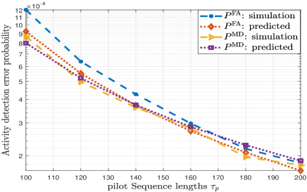
(a)

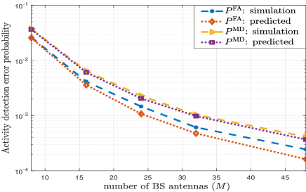
(b)

Figure 1: Probabilities of miss detection and false alarm obtained by the AMP algorithm (simulation) and the derived theoretical results (predicted) versus: a) pilot length $\tau_{\mathrm{p}}$, b) number of BS antennas $M$.

Fig. 2 illustrates the channel estimation performance in terms of normalized average square error (NASE), defined as $\textstyle\frac{\mathbb{E}\left[\|{\bf{X}}_{\mathcal{S}}-\hat{{\bf{X}}}_{\mathcal{S}}\|_{\mathrm{F}}^{2}\right]}{\mathbb{E}\left[\|{\bf{X}}_{\mathcal{S}}\|_{\mathrm{F}}^{2}\right]}$, where the expectation is computed via Monte-Carlo averaging over all sources of randomness and $\mathcal{S}$ denotes the set of true active UEs. Fig. 2 compares AMP with two algorithms: 1) the oracle MMSE estimator, which is provided “oracle” knowledge on $\mathcal{S}$, and 2) IRW-ADMM proposed in [8], where the JUICE is formulated as an iterative reweighted $\ell_{2,1}$-norm minimization and solved via the alternating direction method of multipliers. Fig. 2 shows that AMP outperforms significantly IRW-ADMM and it provides near-optimal NASE performance as it approaches the lower bound obtained by the oracle MMSE estimator. This result highlights the gain obtained by using rich side information at the BS: while IRW-ADMM operates only on the mere fact that the effective channel is sparse, AMP utilizes both channel and noise statistics, leading to better channel estimation performance.

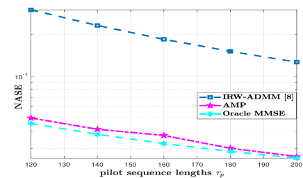
Figure 2: Channel estimation performance in terms of NASE versus pilot length $\tau_{\mathrm{p}}$ for $M=32$, and ${\text{SNR}=10}$ dB.

VI Conclusion

This paper presented an AMP-based solution for the JUICE problem in mMTC under spatially correlated fading channels. By utilizing the properties of the state evolution of the AMP algorithm, the paper derived closed-form expression for both the miss detection and false alarm probabilities. The simulation experiments showed that the theoretical analysis provided in this paper matched the numerical results.

References

- [1] A. C. Cirik, N. M. Balasubramanya, L. Lampe, G. Vos, and S. Bennett, “Toward the standardization of grant-free operation and the associated NOMA strategies in 3GPP,” IEEE Commun. Stand. Mag., vol. 3, no. 4, pp. 60–66, 2019.
- [2] Z. Chen, F. Sohrabi, and W. Yu, “Sparse activity detection for massive connectivity,” IEEE Trans. Signal Processing, vol. 66, no. 7, pp. 1890–1904, 2018.
- [3] L. Liu and W. Yu, “Massive connectivity with massive MIMO—part I: Device activity detection and channel estimation,” IEEE Trans. Signal Processing, vol. 66, no. 11, pp. 2933–2946, 2018.
- [4] ——, “Massive connectivity with massive MIMO—part II: Achievable rate characterization,” IEEE Trans. Signal Processing, vol. 66, no. 11, pp. 2947–2959, 2018.
- [5] K. Senel and E. G. Larsson, “Grant-free massive MTC-enabled massive MIMO: A compressive sensing approach,” IEEE Trans. Commun., vol. 66, no. 12, pp. 6164–6175, 2018.
- [6] M. Ke, Z. Gao, Y. Wu, X. Gao, and R. Schober, “Compressive sensing-based adaptive active user detection and channel estimation: Massive access meets massive MIMO,” IEEE Trans. Signal Processing, vol. 68, pp. 764–779, 2020.
- [7] X. Zhang, Y.-C. Liang, and J. Fang, “Novel Bayesian inference algorithms for multiuser detection in M2M communications,” IEEE Trans. Veh. Technol., vol. 66, no. 9, pp. 7833–7848, 2017.
- [8] H. Djelouat, M. Leinonen, and M. Juntti, “Iterative reweighted algorithms for joint user identification and channel estimation in spatially correlated massive MTC,” in Proc. IEEE Int. Conf. Acoust., Speech, Signal Processing, 2021, pp. 4805–4809.
- [9] H. Djelouat, M. Leinonen, L. Ribeiro, and M. Juntti, “Joint user identification and channel estimation via exploiting spatial channel covariance in mMTC,” IEEE Wireless Commun. Lett, vol. 10, no. 4, pp. 887–891, 2021.
- [10] H. Djelouat, M. Leinonen, and M. Juntti, “Spatial correlation aware compressed sensing for user activity detection and channel estimation in massive MTC,” arXiv preprint arXiv:2104.08508, 2021.
- [11] Y. Cui, S. Li, and W. Zhang, “Jointly sparse signal recovery and support recovery via deep learning with applications in MIMO-based grant-free random access,” IEEE J. Select. Areas Commun., vol. 39, no. 3, pp. 788–803, 2021.
- [12] E. Björnson, L. Sanguinetti, and M. Debbah, “Massive MIMO with imperfect channel covariance information,” in Proc. Annual Asilomar Conf. Signals, Syst., Comp., 2016, pp. 974–978.
- [13] Y. Cheng, L. Liu, and L. Ping, “Orthogonal AMP for massive access in channels with spatial and temporal correlations,” IEEE J. Select. Areas Commun., vol. 39, no. 3, pp. 726–740, 2021.
- [14] A. Laya, L. Alonso, and J. Alonso-Zarate, “Is the random access channel of LTE and LTE-A suitable for M2M communications? a survey of alternatives,” IEEE Commun. Surveys & Tutorials, vol. 16, no. 1, pp. 4–16, 2013.
- [15] P. Schniter, “A simple derivation of AMP and its state evolution via first-order cancellation,” IEEE J. Select. Topics Signal Processing, vol. 68, pp. 4283–4292, 2020.
- [16] D. L. Donoho, A. Maleki, and A. Montanari, “Message-passing algorithms for compressed sensing,” Proceedings of the National Academy of Sciences, vol. 106, no. 45, pp. 18 914–18 919, 2009.
- [17] J. Ziniel and P. Schniter, “Efficient high-dimensional inference in the multiple measurement vector problem,” IEEE Trans. Signal Processing, vol. 61, no. 2, pp. 340–354, 2012.
- [18] J. Kim, W. Chang, B. Jung, D. Baron, and J. C. Ye, “Belief propagation for joint sparse recovery,” arXiv preprint arXiv:1102.3289, 2011.
- [19] A. M. Mathai and S. B. Provost, Quadratic forms in random variables: theory and applications. Dekker, 1992.
- [20] E. Björnson, J. Hoydis, and L. Sanguinetti, “Massive MIMO networks: Spectral, energy, and hardware efficiency,” Foundations and Trends® in Signal Processing, vol. 11, no. 3-4, pp. 154–655, 2017. [Online]. Available: http://dx.doi.org/10.1561/2000000093