Bayesian Modeling of Effective and Functional Brain Connectivity using Hierarchical Vector Autoregressions

Abstract

Analysis of brain connectivity is important for understanding how information is processed by the brain. We propose a novel Bayesian vector autoregression (VAR) hierarchical model for analyzing brain connectivity in a resting-state fMRI data set with autism spectrum disorder (ASD) patients and healthy controls. Our approach models functional and effective connectivity simultaneously, which is new in the VAR literature for brain connectivity, and allows for both group- and single-subject inference as well as group comparisons. We combine analytical marginalization with Hamiltonian Monte Carlo (HMC) to obtain highly efficient posterior sampling. The results from more simplified covariance settings are, in general, overly optimistic about functional connectivity between regions compared to our results. In addition, our modeling of heterogeneous subject-specific covariance matrices is shown to give smaller differences in effective connectivity compared to models with a common covariance matrix to all subjects.

, and

1 Introduction

The use of functional magnetic resonance imaging (fMRI) to investigate brain connectivity dates back to seminal papers from the mid-1990:s (Friston 1994, Biswal et al. 1995), and during the last decade the interest has increased dramatically (Solo et al. 2018). Brain connectivity is an important tool in understanding how information is processed by the brain, with applications in both non-clinical and clinical settings. On the clinical side, connectivity is frequently investigated in association with different kinds of neuropsychological conditions, e.g. schizophrenia (Lynall et al. 2010), ADHD (Konrad and Eickhoff 2010), epilepsy (Morgan, Abou-Khalil and Rogers 2015) and autism spectrum disorder (ASD) (Easson, Fatima and McIntosh 2019). The most common approach for studying brain connectivity using fMRI is so-called resting state fMRI (rs-fMRI), and the analyses are mainly divided into functional and effective connectivity. Functional connectivity pertains to the investigation of undirected associations between brain regions, whereas effective connectivity refers to directed associations (Friston 1994, 2011). Our work targets both functional and effective connectivity, which is new in the literature, and the possibility to perform both group-level inference, which is most common and important in practice, as well as subject-specific inference.

In an rs-fMRI scan, the subject is typically scanned for around ten minutes or less, without specific instructions or tasks to complete. The brain is divided into three-dimensional pixels, called voxels, with a side of about 3-4 mm. Within each voxel, the blood oxygenation level depend (BOLD) signal is measured, which is a proxy measure for neural activity. The BOLD signal in every voxel is usually sampled at about 0.5-2 seconds intervals; for a rigorous and detailed introduction to fMRI, see Buxton (2009). The data obtained are therefore voxelwise time series, where the time series length is usually 200-1000 observations. The number of voxels tend to be in the hundreds of thousands, and some kind of dimension reduction is therefore typically used to divide the brain into at most a few hundred functional regions using a brain atlas, see e.g. Power et al. (2011) or Glasser et al. (2016). A single time series for each region is then constructed by e.g. averaging the time series for all voxels within the region. Our work assumes the rs-fMRI data has been preprocessed to yield such regionwise time series.

The overarching statistical problem in functional and effective connectivity analysis is to estimate suitable measures of association between brain regions. The perhaps simplest solution, which is still widely used in practice, is to calculate the pairwise Pearson correlation, or partial correlation, between every pair of regions. These approaches have the obvious drawback of completely disregarding autoregressive dependencies, both within and between regions. Afyouni, Smith and Nichols (2019) point out that the standard error of the sample correlation coefficient becomes biased from autocorrelation, which implies that the commonly used Fisher transformation can not stabilise the variance.

Attention has therefore turned to time series modeling, e.g. wavelet expansions (Zhang et al. 2014) and vector autoregressive (VAR) models either in the time domain (Chiang et al. 2017, Goebel et al. 2003), or in the frequency domain (Cassidy, Rae and Solo 2015; Cassidy et al. 2018). Dynamic Causal Models (DCM, Friston, Harrison and Penny 2003), a state-space model with ambitious neurophysiological modeling have been extended from task fMRI data to analyze connectivity from resting-state data (Friston et al. 2014).

We propose a Bayesian hierarchical VAR model for both effective and functional connectivity that accounts for autoregressive dependencies within and between brain regions. The hierarchical setting allows for comparison of group-level inference in a straightforward manner. Our results differ substantially from other comparable VAR models in the brain connectivity literature. In general, the results from more simplified covariance settings overestimate functional connectivity between regions compared to our results. We also observe smaller differences in EC, which we suspect are mainly due to heterogeneous subject-specific covariance matrices, which other approaches with a common covariance matrix for all subjects can not account for. We fit these more complex and computationally very demanding models by integrating out the subject-specific parameters to obtain posterior inference on the group-level parameters using highly efficient Hamiltonian Monte Carlo (HMC) sampling. The article is organized as follows. In Section 2, we define our proposed model with subject-specific covariance matrices, and models with more simplified covariance settings (Chiang et al. (2017) and Gorrostieta et al. (2012, 2013)). Our Bayesian setting is described and posterior inference is derived in Section 3. Group-level inference on a real rs-fMRI data set with controls and individuals diagnosed with ASD is presented in Section 4. Concluding remarks are given in Section 5.

2 A Bayesian VAR hierarchical modeling for Brain Connectivity

This section describes a Bayesian vector autoregressive (VAR) hierarchical model for brain connectivity applied to a group of subjects. The model allows for subject-specific VAR parameters centered around a group-level VAR. We also discuss two special cases of our model which have been used for effective connectivity by Chiang et al. (2017) and Gorrostieta et al. (2012, 2013). Section 3 proposes an efficient posterior sampling algorithm for the model that combines analytical marginalization with HMC.

2.1 The hierarchical VAR model

Let $Y_{rst}$ be the fMRI BOLD signal for subject $s$ in region $r$ at time $t$, where $r=1,\dots,R,$ $s=1,\dots,S,$ and $t=1,\dots,T$. The Bayesian VAR (BVAR) model of order $L$ can be defined for

$$Y_{s,t}=\left[\begin{array}[]{c}Y_{1st}\\ \vdots\\ Y_{Rst}\end{array}\right],B_{ls}=\left[\begin{array}[]{ccc}B_{11ls}&\cdots&B_{1Rls}\\ \vdots&\ddots&\vdots\\ B_{R1ls}&\cdots&B_{RRls}\end{array}\right],B_{s}=\left(B_{1s},\dots,B_{Ls}\right)$$

as

$$Y_{s,t}=\sum_{l=1}^{L}B_{ls}Y_{s,t-l}+\epsilon_{st},\;\epsilon_{st}\sim N_{R}\left(0,\Sigma_{s}\right)$$

$$\textrm{vec}\left(B_{s}\right)|\Sigma_{s}\sim N_{LR^{2}}\left(\textrm{vec}\left(B\right),\Sigma_{s}\otimes P_{s}^{-1}\right)$$

$$\Sigma_{s}\sim IW\left(\nu\Sigma,\nu\right),\;f\left(\nu\right)\propto 1,\,\nu>R+1$$

$$\textrm{vec}\left(B\right)|\Sigma\sim N\left(B_{0},\Sigma\otimes P_{0}^{-1}\right)$$ (1)

$$\Sigma\sim IW\left(\nu_{0}\Psi_{0},\nu_{0}\right),$$

where $N_{k}\left(\right)$ and $IW\left(\right)$ denote the $k$-dimensional multivariate normal and inverse Wishart distributions, respectively. Thus, the user needs to specify prior precision matrices $P_{0}$, $\Psi_{0}$, $P_{s}$ for $s=1,\ldots,S$´, and the degrees of freedom $\nu_{0}>R+1$. We elaborate on our chosen prior specification in Section 3.3. We label the general hierarchical VAR in (1) as Model 1.

The global parameters $B$ and $\Sigma$ in (1) are of main interest, in particular comparing the connectivity implied by $B$ and $\Sigma$ between groups of subjects; see the application in Section 4 where a group of subjects diagnosed with autism spectrum disorder (ASD) are compared to healthy controls.

We also consider the following two submodels of Model 1. First, Model $2$ assumes a common covariance matrix for all subjects, i.e. $\Sigma_{s}=\Sigma$ for all $s$. This model is clearly nested in Model $1$, since

$$\left(\Sigma_{s}\right)_{\nu}\overset{d}{\longrightarrow}\Sigma\text{ as }\nu\longrightarrow\infty.$$

Model 3 makes the additional simplification also made by Chiang et al. (2017) and Gorrostieta et al. (2012, 2013); that the common covariance matrix $\Sigma$ is diagonal with prior independent diagonal elements following a conjugate inverse gamma ($IG$) distribution (Press 2005),

$$\Sigma_{rr}\sim IG\left(\frac{\nu_{0}-2R}{2},\frac{\nu_{0}\Psi_{0rr}}{2}\right).$$

Hence, Model 3 does not allow estimation of functional connectivity from non-zero off-diagonal elements of $\Sigma$.

3 Bayesian Inference

The Bayesian approach updates a prior distribution for all model parameters with observed data through the likelihood function to a posterior distribution

$$p\left(B_{1:S},\Sigma_{1:S},B,\Sigma|Y\right)\propto p\left(Y|B_{1:S},\Sigma_{1:S},B,\Sigma\right)p\left(B_{1:S},\Sigma_{1:S},B,\Sigma\right),$$ (2)

where $B_{1:S}=\{B_{1},\ldots,B_{S}\}$, and $\Sigma_{1:S}$ is defined analogously. The object of main interest is the marginal posterior of the group-level parameters

$$p\left(B,\Sigma|Y\right)\propto p\left(Y|B,\Sigma\right)p\left(B,\Sigma\right),$$ (3)

which is obtained by integrating out the subject-specific parameters from (2). The marginal posterior distribution in Model 2, i.e. the model with common $\Sigma$ for all subjects, can be derived in closed form. However, the posterior for the general model where all parameters are subject-specific is not tractable. We propose an efficient HMC algorithm to sample from the marginal posterior in (3). The analytical result for Model 2 is also exploited for determining the prior hyperparameters in Model 1.

3.1 Posterior inference when $\Sigma$ is common to all subjects

Let $X_{s}=\left(Y_{s,t-1},\dots,Y_{s,t-L}\right)$ be the set of covariates in the BVAR model. The likelihood function of $\left(B_{s},\Sigma\right)$ for each subject $s$ is given by (see Appendix A for details)

$$p\left(Y_{s}|B_{s},\Sigma,X_{s}\right)=\left|2\pi\Sigma\right|^{-n/2}\exp\left(-\frac{1}{2}\textrm{tr}\Sigma^{-1}V_{s}\right)$$ (4)

$$\times\exp\left(-\frac{1}{2}\left(B_{s}-\hat{B_{s}}\right)^{T}\left(\Sigma^{-1}\otimes X_{s}^{T}X_{s}\right)\left(B_{s}-\hat{B_{s}}\right)\right),$$

where $n=T-L$, $V_{s}=\left(Y_{s}-X_{s}\hat{B_{s}}\right)^{T}\left(Y_{s}-X_{s}\hat{B_{s}}\right)$ and $\hat{B_{s}}=\left(X_{s}^{T}X_{s}\right)^{-1}X_{s}^{T}Y_{s}.$ The marginal likelihood function of $\left(B,\Sigma\right)$ for all subjects is given by

$$\prod_{s=1}^{S}p\left(Y_{s}|B,\Sigma,X_{s}\right)=\prod_{s=1}^{S}\int p\left(Y_{s}|B_{s},\Sigma,X_{s}\right)p\left(B_{s}|\Sigma\right)dB_{s}.$$

Multiplying this marginal likelihood with the prior distribution of $\left(B,\Sigma\right)$, the posterior distribution of $\left(B,\Sigma\right)$ becomes (see Appendix A for details)

$$p\left(B,\Sigma|Y_{s},X_{s}\right)=c_{0}c_{\kappa}\left|P_{0}\right|^{p/2}\left|\Sigma\right|^{-\left(Sn+\nu_{0}+p+1\right)/2}\exp\left(-\frac{1}{2}\textrm{tr}\Psi_{n}\Sigma^{-1}\right)$$ (5)

$$\times\exp\left(-\frac{1}{2}\textrm{tr}\Sigma^{-1}\left(B-\tilde{B}\right)^{T}\tilde{P}\left(B-\tilde{B}\right)\right),$$

where $c_{0}$ does not depend on $B$ and $\Sigma,$ $c_{\kappa}=\prod_{s=1}^{S}c_{\kappa_{s}}=\prod_{s=1}^{S}\left(\left|P_{s}\right|^{p/2}\left|P_{s}+X_{s}^{T}X_{s}\right|^{-p/2}\right)$, $\Psi_{n}=\nu_{0}\Psi_{0}+\sum_{s=1}^{S}\left(R_{s}+E_{s}^{T}Q_{s}^{-1}E_{s}\right)+B_{0}^{T}P_{0}B_{0}-\tilde{B}^{T}\tilde{P}\tilde{B},$
$\tilde{P}=P_{0}+\sum_{s=1}^{S}Q_{s}^{-1},$ $\tilde{B}=\tilde{P}^{-1}\left(P_{0}B_{0}+\sum_{s=1}^{S}Q_{s}^{-1}E_{s}\right),$
$R_{s}=\left(Y_{s}-X_{s}K_{1s}X_{s}^{T}Y_{s}\right)^{T}\left(Y_{s}-X_{s}K_{1s}X_{s}^{T}Y_{s}\right)+Y_{s}^{T}X_{s}K_{1s}P_{s}K_{1s}X_{s}^{T}Y_{s}-E_{s}^{T}Q_{s}^{-1}E_{s}$,
$K_{1s}=\left(P_{s}+X_{s}^{T}X_{s}\right)^{-1},$ $Q_{s}=\left(P_{s}K_{1s}X_{s}^{T}X_{s}K_{1s}P_{s}+\left(I-K_{1s}P_{s}\right)^{T}P_{s}\left(I-K_{1s}P_{s}\right)\right)^{-1},$
$E_{s}=Q_{s}\left(P_{s}K_{1s}X_{s}^{T}\left(Y_{s}-X_{s}K_{1s}X_{s}^{T}Y_{s}\right)+\left(I-K_{1s}P_{s}\right)^{T}P_{s}K_{1s}X_{s}^{T}Y_{s}\right)$ and $I$ is the identity matrix.

Conditional on $\Sigma$ the posterior distribution of $B$ is given by

$$B|\Sigma,\boldsymbol{Y}\sim N_{p,q}\left(\tilde{B},\tilde{P}^{-1},\Sigma\right),$$

i.e. a matrix-Normal distribution with posterior mean $\tilde{B}$ as a weighted average of the data mean $B_{D}=\left(\sum_{s=1}^{S}Q_{s}^{-1}\right)^{-1}\sum_{s=1}^{S}Q_{s}^{-1}E_{s}$ and prior mean $B_{0}$. Integrating out $B$, the marginal posterior distribution of $\Sigma$ is

$$\Sigma|\boldsymbol{Y}\sim IW\left(\Psi_{n},\,\nu_{n}\right),$$

where $\nu_{n}=\nu_{0}+Sn-q.$ Hence, the marginal posterior distribution of $\Sigma$ is an Inverse-Wishart distribution with $\nu_{n}$ degrees of freedom and scale matrix $\Psi_{n}$ in Model 2. This implies for Model 3 that the marginal posterior distribution of each element $rr$ in the diagonal matrix $\Sigma$ follows an inverse gamma distribution as (Press 2005)

$$\Sigma_{rr}|\boldsymbol{Y}\sim IG\left(\frac{\nu_{n}-2R}{2},\frac{\nu_{n}\Psi_{nrr}}{2}\right).$$

3.2 Posterior inference for the hierarchical VAR with subject-specific $\Sigma_{s}$

Replacing $\Sigma$ with $\Sigma_{s}$ in Equation (4) gives the likelihood function of $\left(B_{s},\Sigma_{s}\right)$ for each subject $s$. Then, the marginal likelihood function of $\left(B,\Sigma,\nu\right)$ becomes (see Appendix B for details)

$$p\left(Y|B,\Sigma,\nu,X\right)=\prod_{s=1}^{S}\int\int p\left(Y_{s}|B_{s},\Sigma_{s},X_{s}\right)p\left(B_{s},\Sigma_{s}|B,\Sigma\right)dB_{s}d\Sigma_{s}$$

$$=c_{1}\left|\nu\Sigma\right|^{\nu/2}\prod_{s=1}^{S}\left|\nu\Sigma+R_{s}+\left(B-E_{s}\right)^{T}Q_{s}^{-1}\left(B-E_{s}\right)\right|^{-\left(n+\nu\right)/2},$$

where $c_{1}$ does not depend on $B$, $\Sigma,$ and $\nu$. The posterior distribution of $\left(B,\Sigma,\nu\right)$ is intractable and high-dimensional, so we use the HMC algorithm with hyperparameters tuned adaptively using the No-U-Turn Sampler (NUTS) (Hoffman and Gelman, 2014) to sample from the posterior. We implement the algorithm in the probabilistic programming language Stan, see Appendix C for the Stan model specification. To monitor convergence to the posterior, we run three parallel MCMC chains until the diagnostic convergence measure $\hat{R}$ in Gelman and Rubin (1992) is close to $1$.

3.3 Prior specification

Let $\textrm{max }s_{r}^{2}$ be the maximum sample variance in region $r$ for all subjects. We choose a non-informative prior for $\Sigma$ by letting $\Psi_{0}$ in (1) be a diagonal matrix with elements $\Psi_{0rr}=\textrm{max }s_{r}^{2},\;r=1,\dots,R,$ and a low degree of freedom $\nu_{0}=R+2$. Following Litterman (1986), it is common practice in the BVAR literature to impose heavier shrinkage on higher lag orders. To implement this effect we let $P_{0}^{-1}=\lambda D$ and $P_{s}^{-1}=\kappa_{s}D$ for each subject $s$, where the diagonal elements of $D$ for lag $l$ are given by $\left(l^{2}\bar{s_{r}^{2}}\right)^{-1},$ where $\bar{s_{r}^{2}}$ is the mean of the subjects’ sample variances in region $r$.

The values of $\lambda$ and $\kappa_{s}$ are obtained from an empirical Bayes approach by maximizing the analytical, tractable, marginal likelihood of $Y$ in Model $2$. This is expected to be a good approximation to the optimal hyperparameters for Model 1 since $\lambda$ and $\kappa_{s}$ are not related to $\Sigma$ or $\Sigma_{s}$, which is the aspect that differs between Models 1 and 2. Integrating out $\left(B,\Sigma\right)$ from the posterior distribution in Equation (5), the marginal likelihood of the data $\boldsymbol{Y}$ can be written as a function of $\lambda$ and $\kappa=\left(\kappa_{1},\dots,\kappa_{S}\right)$ as

$$f\left(\boldsymbol{Y},\kappa,\lambda\right)=c_{2}c_{\kappa}\left|P_{0}\right|^{p/2}\left|\tilde{P}\right|^{-p/2}\left|\Psi_{n}\right|^{-\frac{1}{2}\left(Sn-q+\nu_{0}\right)},$$

where $c_{2}$ does not depend on $\kappa$ and $\lambda$. Optimizing this function with respect to $\lambda$ and $\kappa$, gives the estimated values of the hyperparameters in the prior precision matrices $P_{0}$ and $P_{s}$ of all models, respectively.

4 Brain Connectivity in resting-state fmri data

In Section 4.1, we describe the data used for group comparisons between healthy controls and individuals diagnosed with ASD. Effective and functional connectivity results are presented and compared between the models in Section 4.2. In Section 4.3, we present a brief overview of computational time requirements for analyzing the data with different number of time lags and number of regions considered.

4.1 Description of data and ROI selection

We use data from ABIDE (Di Martino et al., 2014) preprocessed (Craddock et al., 2013) consisting of resting state fMRI data from 539 individuals diagnosed with ASD and 573 healthy controls; we use randomly selected subsets of 20 controls and 20 ASD patients from the data collected at New York University. The fMRI data were collected using a 3 T Siemens Allegra scanner using a TR of 2 seconds. Each fMRI dataset contains 180 time points. No motion scrubbing has been performed, but the first four volumes were dropped in the processing to obtain 176 time points. The ABIDE Preprocessed data have been processed with four different pipelines, and we use the data from the CCS (connectome computation system) pipeline here. We use the data preprocessed without global signal regression and without bandpass filtering, as bandpass filtering will substantially change the autoregressive structure and we prefer to model it. Interested readers are referred to ABIDE preprocessed for preprocessing details. As all the preprocessed data are freely available, other researchers can reproduce our findings.

We select the ROI:s guided by Easson, Fatima and McIntosh (2019), as their rs-fMRI dataset also included ASD patients and healthy controls. We include regions belonging to networks which are active during resting-state scans for both groups, as well as there being some indication of between-group differences in network configuration. The present analyses use ten regions (five in each hemisphere) belonging to the Default-Mode Network (DMN) and ten regions (also here five in each hemisphere) belonging to the Sensory-Motor Network (SMN). More details on the selected regions are given in Appendix D. To make graphs more readable, we refer to the 20 brain regions by numbering them as R1-R20 instead of naming them in the graphs (see Appendix D for a full list of region locations). Regions R1-R10 belong to the DMN and regions R11-R20 to the SMN.

4.2 Results on effective and functional connectivity

We present results on both effective (EC) and functional (FC) connectivity for the three models in Section 2, using the data described in Section 4.1. The EC and FC results are presented for two time lags ($L=2$) for each BVAR model, which is the optimal number of lags for Model 1 by the widely applicable information criterion (WAIC, Vehtari, Gelman and Gabry (2017)), see Table 1. Models with two time lags for rs-fMRI data have also been suggested previously in the literature (Chiang et al. 2017, Gorrostieta et al. 2012, 2013).

			Controls				ASDS
		Model 1	Model 2	Model 3		Model 1	Model 2	Model 3
$L=1$		641306	646658	669358		645569	652108	674576
$L=2$		641158	646460	669078		645288	651764	673966
$L=3$		641179	646469	669109		645360	651769	673830

Table 1: WAIC information criteria for the three models with $p=20$ regions and different lag lengths $L$.

In addition, note that Model 1 is superior to Model 2 and 3 for each lag and group with substantially lower values of WAIC. Hence, the results clearly suggest that the heterogeneous subject-specific covariance matrices in Model 1 are indeed needed for modeling this data. .

Results on EC corresponds to posterior inference on the AR-coefficients in our Bayesian VAR models. For illustration purposes, we apply thresholds on the posterior distribution of the AR-coefficients, where the threshold is applied on both size of the coefficient and whether a 90 or 95 % credible interval includes zero or not. We show results on EC for each of the ASD and control groups separately, as well as the group differences in EC at different time lags. Results for the separate groups are seen in Figures 1 (control group) and 2 (ASD group).

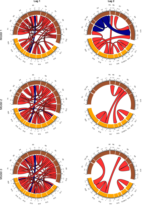
Figure 1: Control group EC: Effective connections, measured by AR coefficients, for the first (left column) and second (right column) time lag for each of our three models (rows one, two and three, respectively). The regions in the DMN are R1-R10 (brown), regions R11-R20 (orange) are the SMN regions. Thresholds for the first time lag were set to the following: connections for which all posterior draws lie above or below zero were kept. For the second time lag we retained connections whose 95% credible intervals do not include zero. The arc length for each region corresponds to the sum of the absolute value of coefficients for the model with the highest sum after thresholding. Direction of connections are indicated with an arrowhead towards the “receiving” region, thickness of the arrow indicate connection strength (coefficient size), and the color of the arrow indicate a positive (red) or negative (blue) coefficient.

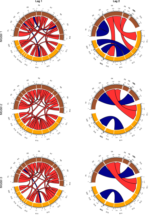
Figure 2: ASD group EC: Effective connections, measured by AR coefficients, the first (left column) and second (right column) time lag for each of our three models (rows one, two and three, respectively). The regions in the DMN are R1-R10 (brown), regions R11-R20 (orange) are the SMN regions. Thresholds for the first time lag were set to the following: connections for which all posterior draws lie above or below zero were kept. For the second time lag we retained connections whose 95% credible intervals do not include zero. The arc length for each region corresponds to the sum of the absolute value of coefficients for the model with the highest sum after thresholding. Direction of connections are indicated with an arrowhead towards the “receiving” region, thickness of the arrow indicate connection strength (coefficient size), and the color of the arrow indicate a positive (red) or negative (blue) coefficient.

Each subgraph gives a visual network description of the thresholded directed connections between regions. The general pattern across groups and models is that there are considerably more connections at one time lag than at two time lags, despite having a stricter threshold at one time lag. There are more connections within a network than between networks, as expected for the definition of the network, and most of the coefficients are positive. For a given time lag, there are some differences between the models. Model 2 and 3 yield more connections than Model 1 for lag 1, while Model 1 yields some additional, mostly negative, connections compared to Model 2 and 3.

Figure 3 illustrates differences in EC between the groups as the difference in corresponding AR-coefficients.

Figure 3: Difference in EC, Control group EC – ASD group EC: Effective connection difference, measured by AR coefficient difference, for one (left column) and two (right column) time lags, for each of our three models (rows one, two and three, respectively). The regions in the DMN are R1-R10 (brown), regions R11-R20 (orange) are the SMN regions. Thresholds for the first time lag was set to the following: connections whose 95% credible intervals do not include zero, were kept. For the second time lag we retained connections whose 95% credible intervals do not include zero. The arc length for each region corresponds to the sum of the absolute value of coefficient difference for the model with the highest sum after thresholding. Direction of connections are indicated with an arrowhead towards the “receiving” region, thickness of the arrow indicate size of coefficient difference, and the color of the arrow indicate a positive (red) or negative (blue) coefficient difference.

Results from Models 2 and 3 indicate substantially more group differences than Model 1 for both time lags, while for a given model the number of differences is greater for lag 1. In the figure, the differences for the two lags look comparable, but note that we use a more leniant threshold for lag 2 for illustrative purposes (otherwise there would have been only one connection for the differences of lag 2). In general, most of the differences are within-network, as for the group-specific connections. There are also some discrepancies in EC between Models 2 and 3, but much less than the corresponding discrepancies between any of these models and Model 1.

Results for FC are shown in Figure 4.

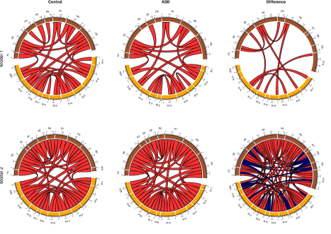
Figure 4: FC for both groups and the group difference in FC, measured by the estimated FC correlation matrix between regions and the FC correlation matrix difference between regions (columns) for Models 1 and 2 (rows). The regions in the DMN are R1-R10 (brown), regions R11-R20 (orange) are the SMN regions. The following thresholding was used in the plot: for the separate groups, the absolute posterior mean correlation was thresholded at 0.35, and all posterior draws lie above or below zero. When considering the group difference, the absolute posterior mean difference had to exceed 0.05 and the 95% credible intervals exclude zero. The arc length for each region corresponds to the sum of the absolute value of the correlations - or the correlation differences - for the model with the highest sum after thresholding. Thickness of the line indicate size of correlation/correlation difference, and the color of the arrow indicate a positive (red) or negative (blue) coefficient/coefficient difference.

We only compare Models 1 and 2, since Model 3 has a diagonal covariance matrix and therefore does not allow estimation of FC. We follow the same procedure as for EC by considering FC for each group separately, as well as the difference in FC between groups. The figures were constructed in a similar manner as for the figures for EC, but FC is undirected such that connection lines between regions are undirected. It is clear that the number of functional connections is considerably different between the models in the figure, where Model 2 yields many more functional connections than Model 1. Hence, it is important to account for heterogeneous subject-specific covariance matrices in Model 1 compared to a common covariance matrix in Model 2 in order to obtain accurate inference on functional connectivity. The overestimation of functional connections in Model 2 also implies an overestimation of group differences, resulting in many spurious functional connections between the groups from Model 2.

We elaborate further on comparing results from the different models by pairwise comparisons of the posterior means of the parameters. In Figure 5, AR-coefficients and the elements of the FC correlation matrix are compared between the models.

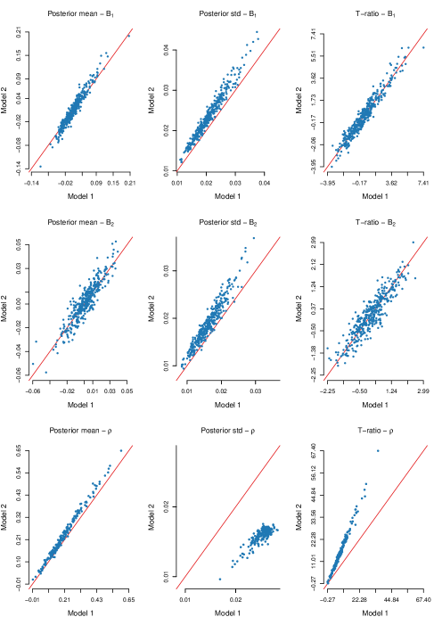
Figure 5: Scatterplots of posterior means, standard deviation and their ratio of AR coefficients and correlations obtained using Models 1 and 2 respectively, as indicated on the axes.

The comparison between Model 1 and 3 was omitted as it is virtually undistinguishable from the Model 1-Model 2 comparison. We only present this comparison for the control group, as the results for the ASD group were very similar. The posterior means of the AR coefficients from Models 1 and 2 are quite close (upper two panels in the left column of Figure 5). The posterior standard deviations of the respective coefficients are slightly higher for Model 2 compared to Model 1 (upper two panels in the middle column), but the t-ratios are quite similar (upper two panels in the right column). Moving on to the bottom row, the posterior means of FC correlations are fairly similar, although Model 1 yields slightly lower posterior mean correlations compared to Model 2. This means that the differences in FC between the Models are mainly due to the standard deviation of the respective posterior distributions being much smaller for Model 2, which is evident in the t-ratios as well.

4.3 Computing times

Table 2 presents computation times for applying the HMC algorithm to the posterior of Model 1 for different numbers of brain regions; the regions are randomly selected for this purpose, since interest here is only on the computing times.

		$p=10$	$p=20$	$p=30$
$L=1$		0.005	0.094	0.479
$L=2$		0.008	0.385	9.242
$L=3$		0.018	1.313	48.805
$L=4$		0.048	5.288	N/A

Table 2: Computation times (hours) for Model $1$ with different lag lengths $L$ and number of regions $p$. The data consists of $S=20$ randomly selected healthy controls and the length of each time series within each region is $T=176$. The computer analyses were run using two parallel MCMC chains with $200$ warm-up and $500$ sampling draws for each chain on two CPUs with a 2.7GHz processor. N/A (not applicable) means that the HMC algorithm took too long time to converge and was therefore interrupted.

Our approach works fine for around 20-30 brain regions compared to previous VAR modeling of 5-6 regions, e.g. Chiang et al. (2017); Gorrostieta et al. (2012, 2013), but becomes very computational demanding for more than $p=30$ regions and at least two time lags.

5 Conclusions

We propose a novel Bayesian VAR hierarchical model for brain connectivity that accounts for autoregressive dependencies within and between brain regions, and apply it to an existing, openly available rs-fMRI data set. Compared to existing Bayesian VAR hierarchical models for this purpose, we incorporate more flexible, subject-specific, covariance modeling that estimates both effective and functional connectivity simultaneously. By using the information criteria WAIC, we show that our proposed model is superior to special cases of our model with a common covariance matrix for all subjects. Similar simplified, diagonal, covariance matrices has been used previously for effective connectivity by Chiang et al. (2017) and Gorrostieta et al. (2012, 2013). We are also able to handle 20-30 brain regions compared to previous VAR modeling in the literature of typically 5-6 regions.

Overall, our flexible model displayed the most conservative results with respect to the number of effective and functional connections deemed to be non-zero from common thresholds. This is especially true for functional connectivity where the special case with a common covariance matrix for all subjects substantially overestimates the number of non-zero connections. We find that the standard deviations of the corresponding posteriors to functional connectivity are much lower for the special model case, which implies that between-subject variation is underestimated in such models.

We suggest some future extensions of our work. Flexible VAR modeling for effective and functional connectivity is not yet ready for large-scale brain connectivity, which typically involves hundreds of brain regions. Our derived, analytical result for the posterior inference of the model with a common covariance matrix for all subjects can be directly applied, but with the obvious drawback of biased inference for effective and, especially, functional connectivity. Another possibility can be to extend our modeling to handle longitudinal data, e.g. repeated rs-fMRI scans over time.

Appendix A Posterior distribution of $\left(B,\Sigma\right)$ for Model 2 with common covariance matrix $\Sigma$

Let $X_{s,t}=\left(Y_{s,t-1},\dots,Y_{s,t-L}\right)$ be the set of covariates in the BVAR model. The likelihood function of $\left(B_{s},\Sigma\right)$ for each subject $s$ is given by

$$p\left(Y_{s}|X_{s},B_{s},\Sigma\right)=\prod_{t=L+1}^{T}\left|2\pi\Sigma\right|^{-1/2}\exp\left(-\frac{1}{2}\left(Y_{s,t}-B_{s}^{T}X_{s,t}\right)^{T}\Sigma^{-1}\left(Y_{s,t}-B_{s}^{T}X_{s,t}\right)\right)$$

$$=\left|2\pi\Sigma\right|^{-n/2}\exp\left(-\frac{1}{2}\textrm{tr}\Sigma^{-1}\left(Y_{s}-X_{s}B_{s}\right)^{T}\left(Y_{s}-X_{s}B_{s}\right)\right).$$

Completing the squares of $B_{s}$, the likelihood function of $\left(B_{s},\Sigma\right)$ can be written as

$$p\left(Y_{s}|X_{s},B_{s},\Sigma\right)=\left|2\pi\Sigma\right|^{-n/2}\exp\left(-\frac{1}{2}\textrm{tr}\Sigma^{-1}V_{s}\right)\exp\left(-\frac{1}{2}\textrm{tr}\left(B_{s}-\hat{B_{s}}\right)^{T}X_{s}^{T}X_{s}\left(B_{s}-\hat{B_{s}}\right)\Sigma^{-1}\right),$$

where $n=T-L$, $V_{s}=\left(Y_{s}-X_{s}\hat{B_{s}}\right)^{T}\left(Y_{s}-X_{s}\hat{B_{s}}\right)$ and $\hat{B_{s}}=\left(X_{s}^{T}X_{s}\right)^{-1}X_{s}^{T}Y_{s}.$ Then, using the identity

$$\textrm{tr}\left(A_{1}^{T}A_{2}A_{3}A_{4}^{T}\right)=\left(\textrm{vec}A_{1}\right)^{T}\left(A_{4}\otimes A_{2}\right)\left(\textrm{vec}A_{3}\right)$$

with $A_{1}=A_{3}=B_{s}-\hat{B_{s}}$, $A_{2}=X_{s}^{T}X_{s}$, $A_{4}=\Sigma^{-1},$ the likelihood function of $\left(B_{s},\Sigma\right)$ becomes

$$p\left(Y_{s}|X_{s},B_{s},\Sigma\right)=\left|2\pi\Sigma\right|^{-n/2}\exp\left(-\frac{1}{2}\textrm{tr}\Sigma^{-1}V_{s}\right)\exp\left(-\frac{1}{2}\left(B_{s}-\hat{B_{s}}\right)^{T}\left(\Sigma^{-1}\otimes X_{s}^{T}X_{s}\right)\left(B_{s}-\hat{B_{s}}\right)\right).$$

The marginal likelihood function of $\left(B,\Sigma\right)$ for all subjects becomes

$$\prod_{s=1}^{S}p\left(Y_{s}|B,\Sigma,X_{s}\right)=\prod_{s=1}^{S}\int p\left(Y_{s}|X_{s},B_{s},\Sigma\right)p\left(B_{s}|\Sigma\right)dB_{s}$$

$$=c_{0}\prod_{s=1}^{S}c_{\kappa}\left|\Sigma\right|^{-n/2}\exp\left(-\frac{1}{2}\textrm{tr}\Sigma^{-1}\left[\tilde{V_{s}}+\left(\tilde{B_{s}}-B\right)^{T}P_{s}\left(\tilde{B_{s}}-B\right)\right]\right),$$

where $c_{\kappa}=\prod_{s=1}^{S}c_{\kappa_{s}}=\prod_{s=1}^{S}\left(\left|P_{s}\right|^{p/2}\left|P_{s}+X_{s}^{T}X_{s}\right|^{-p/2}\right),$ $\tilde{V_{s}}=\left(Y_{s}-X_{s}\tilde{B}_{s}\right)^{T}\left(Y_{s}-X_{s}\tilde{B}_{s}\right),$ $\tilde{B_{s}}=\left(P_{s}+X_{s}^{T}X_{s}\right)^{-1}\left(X_{s}^{T}Y_{s}+P_{s}B\right),$ and $c_{0}$ is a constant that does not depend on $B$ and $\Sigma$. Rewriting this marginal likelihood on a quadratic form of $B$ and then multiplying the marginal likelihood with the prior distribution of $\left(B,\Sigma\right)$, the posterior distribution of $\left(B,\Sigma\right)$ becomes

$$p\left(B,\Sigma|Y_{s},X_{s}\right)=c_{0}c_{\kappa}\left|P_{0}\right|^{p/2}\left|\Sigma\right|^{-\left(Sn+\nu_{0}+p+1\right)/2}\exp\left(-\frac{1}{2}\textrm{tr}\Sigma^{-1}\left(\nu_{0}\Psi_{0}+\left(B-B_{0}\right)^{T}P_{0}\left(B-B_{0}\right)\right)\right)$$

$$\times\prod_{s=1}^{S}\exp\left(-\frac{1}{2}\textrm{tr}\Sigma^{-1}\left[R_{s}+\left(B-E_{s}\right)^{T}Q_{s}^{-1}\left(B-E_{s}\right)\right]\right),$$

where $R_{s}=\left(Y_{s}-X_{s}K_{1s}X_{s}^{T}Y_{s}\right)^{T}\left(Y_{s}-X_{s}K_{1s}X_{s}^{T}Y_{s}\right)+Y_{s}^{T}X_{s}K_{1s}P_{s}K_{1s}X_{s}^{T}Y_{s}-E_{s}^{T}Q_{s}^{-1}E_{s}$,
$K_{1s}=\left(P_{s}+X_{s}^{T}X_{s}\right)^{-1},$ $Q_{s}=\left(P_{s}K_{1s}X_{s}^{T}X_{s}K_{1s}P_{s}+\left(I-K_{1s}P_{s}\right)^{T}P_{s}\left(I-K_{1s}P_{s}\right)\right)^{-1},$
$E_{s}=Q_{s}\left(P_{s}K_{1s}X_{s}^{T}\left(Y_{s}-X_{s}K_{1s}X_{s}^{T}Y_{s}\right)+\left(I-K_{1s}P_{s}\right)^{T}P_{s}K_{1s}X_{s}^{T}Y_{s}\right),$ and $I$ is the identity matrix.
Rewriting on a quadratic form of $B$, the posterior distribution is finally given by

$$p\left(B,\Sigma|Y_{s},X_{s}\right)=c_{0}c_{\kappa}\left|P_{0}\right|^{p/2}\left|\Sigma\right|^{-\left(Sn+\nu_{0}+p+1\right)/2}\exp\left(-\frac{1}{2}\textrm{tr}\Psi_{n}\Sigma^{-1}\right)$$

$$\times\exp\left(-\frac{1}{2}\textrm{tr}\Sigma^{-1}\left(B-\tilde{B}\right)^{T}\tilde{P}\left(B-\tilde{B}\right)\right),$$

where $\Psi_{n}=\nu_{0}\Psi_{0}+\sum_{s=1}^{S}\left(R_{s}+E_{s}^{T}Q_{s}^{-1}E_{s}\right)+B_{0}^{T}P_{0}B_{0}-\tilde{B}^{T}\tilde{P}\tilde{B},$ $\tilde{P}=P_{0}+\sum_{s=1}^{S}Q_{s}^{-1}$ and $\tilde{B}=\tilde{P}^{-1}\left(P_{0}B_{0}+\sum_{s=1}^{S}Q_{s}^{-1}E_{s}\right)$.

Appendix B Marginal likelihood of $\left(B,\Sigma,\nu\right)$ for Model 1 with subject-specific covariance matrix $\Sigma_{s}$

Replacing $\Sigma$ with $\Sigma_{s}$ in Equation (4) gives the likelihood function of $\left(B_{s},\Sigma_{s}\right)$ for each subject $s$ as

$$p\left(Y_{s}|X_{s},B_{s},\Sigma_{s}\right)=\left|2\pi\Sigma_{s}\right|^{-n/2}\exp\left(-\frac{1}{2}\textrm{tr}\Sigma_{s}^{-1}\left(Y_{s}-X_{s}B_{s}\right)^{T}\left(Y_{s}-X_{s}B_{s}\right)\right).$$

The marginal likelihood function of $\left(B,\Sigma\right)$ for all subjects becomes

$$p\left(Y|B,\Sigma\right)=\prod_{s=1}^{S}p\left(Y_{s}|B,\Sigma,X_{s}\right)=\prod_{s=1}^{S}\int\int p\left(Y_{s}|B_{s},\Sigma_{s},X_{s}\right)p\left(B_{s},\Sigma_{s}\right)dB_{s}d\Sigma_{s}$$

$$=c_{1}\left|\nu\Sigma\right|^{\nu/2}\prod_{s=1}^{S}\left|\nu\Sigma+\tilde{V_{s}}+\left(\tilde{B_{s}}-B\right)^{T}P_{s}\left(\tilde{B_{s}}-B\right)\right|^{-\left(n+\nu\right)/2},$$

where $c_{1}$ is a constant that does not depend on $B$ and $\Sigma$. Rewriting on a quadratic form of $B$ in the determinant, the marginal likelihood of $\left(B,\Sigma\right)$ can be expressed as

$$p\left(Y|B,\Sigma\right)=c\left|\nu\Sigma\right|^{\nu/2}\prod_{s=1}^{S}\left|\nu\Sigma+R_{s}+\left(B-E_{s}\right)^{T}Q_{s}^{-1}\left(B-E_{s}\right)\right|.$$

Appendix C Stan modeling code for Model 1

data {

int<lower=0> p; // number of brain regions

int<lower=0> q; // number of covariates L*p

int<lower=0> S; // number of subjects

int<lower=0> qp; // number of VAR coefficients, qp = q*p

int<lower=0> T; // number of time points

matrix [p,p] R_s[S]; // array with matrices R_s for all subjects

matrix [q,p] E_s[S]; // array with matrices E_s for all subjects

matrix [q,q] Q_s_inv[S]; // array with matrices Q_s_inv for all subjects

// Prior settings

vector[qp] B_0_spec; // prior Mean

cov_matrix[q] Chol_Cov_B; // cholesky decomposition of the covariance matrix for B

int nu_0; // degrees of freedom in the prior for Sigma

cov_matrix[p] Psi_0; // scale matrix in the prior for Sigma

cov_matrix[qp] I_Mat; // identity matrix

}

parameters {

cov_matrix[p] Sigma; // covariance matrix

matrix[q,p] B_spec; // matrix of VAR coefficients

real<lower=p+2> nu; // degrees of freedom in the prior for Sigma_s

}

transformed parameters {

matrix[q,p] B; // matrix of VAR coefficients

B = Chol_Cov_B * B_spec * cholesky_decompose(Sigma);

}

model {

real Sum_logdet;

matrix[p,p] Part_s;

// priors

Sigma ~ inv_wishart(nu_0,Psi_0); // prior for the covariance matrix Sigma

to_vector(B_spec) ~ multi_normal(B_0_spec,I_Mat); // special prior for parameterization

Sum_logdet = 0;

// log-likelihood

for (s in 1:S){

Part_s = nu*Sigma + R_s[s] + quad_form(Q_s_inv[s] , B-E_s[s]);

Sum_logdet = Sum_logdet + log_determinant(Part_s);

}

target += S*( lmgamma(p,0.5*(T+nu)) - lmgamma(p,0.5*nu) );

target += 0.5*S*nu*log_determinant(nu*Sigma) - 0.5*(nu+T)*Sum_logdet;

}

Appendix D ROI information

Information on our selected ROI:s in the Default-Mode Network (DMN) and Sensory-Motor Network (SMN) is given below in the following order: abbreviation in the manuscript, type of network the ROI is classified to, volume of the ROI, $(x,y,z)-$coordinates for the ROI center of mass, and AAL atlas annotation (Tzourio-Mazoyer et al. 2002).

Abbreviation	Network	volume mm^3	center of mass (x,y,z)	AAL annotation
R1	DMN	222	(-6.8;45.7;7.8)	Cingulum_Ant_L
R2	DMN	267	(9.1;-35.9;47.1)	Cingulum_Mid_R
R3	DMN	213	(6.7;42.6;6.1)	Cingulum_Ant_R
R4	DMN	247	(0.3;16.3;32.3)	Cingulum_Mid_L
R5	DMN	249	(-7.9;-33.1;45.5)	Cingulum_Mid_L
R6	DMN	248	(0.0;-0.3;42.2)	Cingulum_Mid_L
R7	DMN	247	(-14.0;-66.3;55.9)	Precuneus_L
R8	DMN	214	(-49.2;22.9;9.3)	Frontal_Inf_Tri_L
R9	DMN	174	(52.1;28.0;4.9)	Frontal_Inf_Tri_R
R10	DMN	266	(10.3;-63.5;56.2)	Precuneus_R
R11	SMN	247	(55.2;-47.5;41.9)	Parietal_Inf_R
R12	SMN	287	(-58.9;-30.2;-2.4)	Temporal_Mid_L
R13	SMN	222	(61.9;-21.1;-15.6)	Temporal_Mid_R
R14	SMN	204	(-47.8;7.9;-9.3)	Insula_R
R15	SMN	210	(-39.7;-12.9;13.3)	Insula_L
R16	SMN	292	(0.4;-15.1;51.8)	Supp_Motor_Area_L
R17	SMN	206	(29.9;-67.5;47.3)	Parietal_Sup_R
R18	SMN	237	(40.7;-11.3;-3.9)	Insula_R
R19	SMN	234	(-33.9;-53.8;49.5)	Parietal_Inf_L
R20	SMN	215	(10.6;1.3;65.9)	Supp_Motor_Area_R

[Acknowledgments]

Anders Eklund is also affiliated with the Center for medical image science and visualization (CMIV).

Anders Lundquist was supported by Riksbankens Jubileumsfond, Grant number P16-028:1. Anders Eklund was supported in part by the Center for Industrial Information Technology (CENIIT) at Linköping University.

References

- Afyouni, Smith and Nichols (2019) {barticle}[author] \bauthor\bsnmAfyouni, \bfnmSoroosh\binitsS., \bauthor\bsnmSmith, \bfnmStephen M\binitsS. M. and \bauthor\bsnmNichols, \bfnmThomas E\binitsT. E. (\byear2019). \btitleEffective degrees of freedom of the Pearson’s correlation coefficient under autocorrelation. \bjournalNeuroImage \bvolume199 \bpages609–625. \endbibitem
- Biswal et al. (1995) {barticle}[author] \bauthor\bsnmBiswal, \bfnmBharat\binitsB., \bauthor\bsnmZerrin Yetkin, \bfnmF.\binitsF., \bauthor\bsnmHaughton, \bfnmVictor M.\binitsV. M. and \bauthor\bsnmHyde, \bfnmJames S.\binitsJ. S. (\byear1995). \btitleFunctional connectivity in the motor cortex of resting human brain using echo-planar mri. \bjournalMagnetic Resonance in Medicine \bvolume34 \bpages537–541. \bdoi10.1002/mrm.1910340409 \endbibitem
- Buxton (2009) {bbook}[author] \bauthor\bsnmBuxton, \bfnmRichard B\binitsR. B. (\byear2009). \btitleIntroduction to functional magnetic resonance imaging: principles and techniques. \bpublisherCambridge university press. \endbibitem
- Cassidy, Rae and Solo (2015) {barticle}[author] \bauthor\bsnmCassidy, \bfnmBen\binitsB., \bauthor\bsnmRae, \bfnmCaroline\binitsC. and \bauthor\bsnmSolo, \bfnmVictor\binitsV. (\byear2015). \btitleBrain Activity: Connectivity, Sparsity, and Mutual Information. \bjournalIEEE Transactions on Medical Imaging \bvolume34 \bpages846–860. \bdoi10.1109/TMI.2014.2358681 \endbibitem
- Cassidy et al. (2018) {barticle}[author] \bauthor\bsnmCassidy, \bfnmBen\binitsB., \bauthor\bsnmBowman, \bfnmF. Dubois\binitsF. D., \bauthor\bsnmRae, \bfnmCaroline\binitsC. and \bauthor\bsnmSolo, \bfnmVictor\binitsV. (\byear2018). \btitleOn the Reliability of Individual Brain Activity Networks. \bjournalIEEE Transactions on Medical Imaging \bvolume37 \bpages649–662. \bdoi10.1109/TMI.2017.2774364 \endbibitem
- Chiang et al. (2017) {barticle}[author] \bauthor\bsnmChiang, \bfnmSharon\binitsS., \bauthor\bsnmGuindani, \bfnmMichele\binitsM., \bauthor\bsnmYeh, \bfnmHsiang J.\binitsH. J., \bauthor\bsnmHaneef, \bfnmZulfi\binitsZ., \bauthor\bsnmStern, \bfnmJohn M.\binitsJ. M. and \bauthor\bsnmVannucci, \bfnmMarina\binitsM. (\byear2017). \btitleBayesian vector autoregressive model for multi-subject effective connectivity inference using multi-modal neuroimaging data. \bjournalHuman Brain Mapping \bvolume38 \bpages1311–1332. \bdoi10.1002/hbm.23456 \endbibitem
- Craddock et al. (2013) {barticle}[author] \bauthor\bsnmCraddock, \bfnmCameron\binitsC., \bauthor\bsnmBenhajali, \bfnmYassine\binitsY., \bauthor\bsnmChu, \bfnmCarlton\binitsC., \bauthor\bsnmChouinard, \bfnmFrancois\binitsF., \bauthor\bsnmEvans, \bfnmAlan\binitsA., \bauthor\bsnmJakab, \bfnmAndrás\binitsA., \bauthor\bsnmKhundrakpam, \bfnmBudhachandra Singh\binitsB. S., \bauthor\bsnmLewis, \bfnmJohn David\binitsJ. D., \bauthor\bsnmLi, \bfnmQingyang\binitsQ., \bauthor\bsnmMilham, \bfnmMichael\binitsM. \betalet al. (\byear2013). \btitleThe neuro bureau preprocessing initiative: open sharing of preprocessed neuroimaging data and derivatives. \bjournalFrontiers in Neuroinformatics \bvolume7. \endbibitem
- Di Martino et al. (2014) {barticle}[author] \bauthor\bsnmDi Martino, \bfnmAdriana\binitsA., \bauthor\bsnmYan, \bfnmChao-Gan\binitsC.-G., \bauthor\bsnmLi, \bfnmQingyang\binitsQ., \bauthor\bsnmDenio, \bfnmErin\binitsE., \bauthor\bsnmCastellanos, \bfnmFrancisco X\binitsF. X., \bauthor\bsnmAlaerts, \bfnmKaat\binitsK., \bauthor\bsnmAnderson, \bfnmJeffrey S\binitsJ. S., \bauthor\bsnmAssaf, \bfnmMichal\binitsM., \bauthor\bsnmBookheimer, \bfnmSusan Y\binitsS. Y., \bauthor\bsnmDapretto, \bfnmMirella\binitsM. \betalet al. (\byear2014). \btitleThe autism brain imaging data exchange: towards a large-scale evaluation of the intrinsic brain architecture in autism. \bjournalMolecular psychiatry \bvolume19 \bpages659–667. \endbibitem
- Easson, Fatima and McIntosh (2019) {barticle}[author] \bauthor\bsnmEasson, \bfnmAmanda K.\binitsA. K., \bauthor\bsnmFatima, \bfnmZainab\binitsZ. and \bauthor\bsnmMcIntosh, \bfnmAnthony R.\binitsA. R. (\byear2019). \btitleFunctional connectivity-based subtypes of individuals with and without autism spectrum disorder. \bjournalNetwork Neuroscience \bvolume3 \bpages344–362. \bdoi10.1162/netn_a_00067 \endbibitem
- Friston (1994) {barticle}[author] \bauthor\bsnmFriston, \bfnmKarl J.\binitsK. J. (\byear1994). \btitleFunctional and effective connectivity in neuroimaging: A synthesis. \bjournalHuman Brain Mapping \bvolume2 \bpages56–78. \bdoi10.1002/hbm.460020107 \endbibitem
- Friston (2011) {barticle}[author] \bauthor\bsnmFriston, \bfnmKarl J\binitsK. J. (\byear2011). \btitleFunctional and effective connectivity: a review. \bjournalBrain Connectivity \bvolume1 \bpages13–36. \bdoi10.1089/brain.2011.0008 \endbibitem
- Friston, Harrison and Penny (2003) {barticle}[author] \bauthor\bsnmFriston, \bfnmK. J.\binitsK. J., \bauthor\bsnmHarrison, \bfnmL.\binitsL. and \bauthor\bsnmPenny, \bfnmW.\binitsW. (\byear2003). \btitleDynamic causal modelling. \bjournalNeuroImage \bvolume19 \bpages1273–1302. \bdoi10.1016/S1053-8119(03)00202-7 \endbibitem
- Friston et al. (2014) {barticle}[author] \bauthor\bsnmFriston, \bfnmKarl J.\binitsK. J., \bauthor\bsnmKahan, \bfnmJoshua\binitsJ., \bauthor\bsnmBiswal, \bfnmBharat\binitsB. and \bauthor\bsnmRazi, \bfnmAdeel\binitsA. (\byear2014). \btitleA DCM for resting state fMRI. \bjournalNeuroImage \bvolume94 \bpages396–407. \bdoi10.1016/j.neuroimage.2013.12.009 \endbibitem
- Gelman and Rubin (1992) {barticle}[author] \bauthor\bsnmGelman, \bfnmAndrew\binitsA. and \bauthor\bsnmRubin, \bfnmDonald B.\binitsD. B. (\byear1992). \btitleInference from Iterative Simulation Using Multiple Sequences. \bjournalStatistical Science \bvolume7 \bpages457–472. \bdoi10.1214/ss/1177011136 \endbibitem
- Glasser et al. (2016) {barticle}[author] \bauthor\bsnmGlasser, \bfnmMatthew F.\binitsM. F., \bauthor\bsnmCoalson, \bfnmTimothy S.\binitsT. S., \bauthor\bsnmRobinson, \bfnmEmma C.\binitsE. C., \bauthor\bsnmHacker, \bfnmCarl D.\binitsC. D., \bauthor\bsnmHarwell, \bfnmJohn\binitsJ., \bauthor\bsnmYacoub, \bfnmEssa\binitsE., \bauthor\bsnmUgurbil, \bfnmKamil\binitsK., \bauthor\bsnmAndersson, \bfnmJesper\binitsJ., \bauthor\bsnmBeckmann, \bfnmChristian F.\binitsC. F., \bauthor\bsnmJenkinson, \bfnmMark\binitsM., \bauthor\bsnmSmith, \bfnmStephen M.\binitsS. M. and \bauthor\bsnmVan Essen, \bfnmDavid C.\binitsD. C. (\byear2016). \btitleA multi-modal parcellation of human cerebral cortex. \bjournalNature \bvolume536 \bpages171–178. \bdoi10.1038/nature18933 \endbibitem
- Goebel et al. (2003) {barticle}[author] \bauthor\bsnmGoebel, \bfnmRainer\binitsR., \bauthor\bsnmRoebroeck, \bfnmAlard\binitsA., \bauthor\bsnmKim, \bfnmDae Shik\binitsD. S. and \bauthor\bsnmFormisano, \bfnmElia\binitsE. (\byear2003). \btitleInvestigating directed cortical interactions in time-resolved fMRI data using vector autoregressive modeling and Granger causality mapping. \bjournalMagnetic Resonance Imaging \bvolume21 \bpages1251–1261. \bdoi10.1016/j.mri.2003.08.026 \endbibitem
- Gorrostieta et al. (2012) {barticle}[author] \bauthor\bsnmGorrostieta, \bfnmCristina\binitsC., \bauthor\bsnmOmbao, \bfnmHernando\binitsH., \bauthor\bsnmBédard, \bfnmPatrick\binitsP. and \bauthor\bsnmSanes, \bfnmJerome N.\binitsJ. N. (\byear2012). \btitleInvestigating brain connectivity using mixed effects vector autoregressive models. \bjournalNeuroImage \bvolume59 \bpages3347–3355. \bdoi10.1016/j.neuroimage.2011.08.115 \endbibitem
- Gorrostieta et al. (2013) {barticle}[author] \bauthor\bsnmGorrostieta, \bfnmCristina\binitsC., \bauthor\bsnmFiecas, \bfnmMark\binitsM., \bauthor\bsnmOmbao, \bfnmHernando\binitsH., \bauthor\bsnmBurke, \bfnmErin\binitsE. and \bauthor\bsnmCramer, \bfnmSteven\binitsS. (\byear2013). \btitleHierarchical vector auto-regressive models and their applications to multi-subject effective connectivity. \bjournalFrontiers in Computational Neuroscience \bvolume7 \bpages1–11. \bdoi10.3389/fncom.2013.00159 \endbibitem
- Hoffman and Gelman (2014) {barticle}[author] \bauthor\bsnmHoffman, \bfnmMatthew D\binitsM. D. and \bauthor\bsnmGelman, \bfnmAndrew\binitsA. (\byear2014). \btitleThe No-U-Turn sampler: adaptively setting path lengths in Hamiltonian Monte Carlo. \bjournalJ. Mach. Learn. Res. \bvolume15 \bpages1593–1623. \endbibitem
- Konrad and Eickhoff (2010) {barticle}[author] \bauthor\bsnmKonrad, \bfnmKerstin\binitsK. and \bauthor\bsnmEickhoff, \bfnmSimon B.\binitsS. B. (\byear2010). \btitleIs the ADHD brain wired differently? A review on structural and functional connectivity in attention deficit hyperactivity disorder. \bjournalHuman Brain Mapping \bvolume31 \bpages904–916. \bdoi10.1002/hbm.21058 \endbibitem
- Litterman (1986) {barticle}[author] \bauthor\bsnmLitterman, \bfnmRobert B.\binitsR. B. (\byear1986). \btitleForecasting With Bayesian Vector Autoregressions - Five Years of Experience. \bjournalJournal of Business & Economic Statistics \bvolume4 \bpages25–38. \bdoi10.1080/07350015.1986.10509491 \endbibitem
- Lynall et al. (2010) {barticle}[author] \bauthor\bsnmLynall, \bfnmM. E.\binitsM. E., \bauthor\bsnmBassett, \bfnmD. S.\binitsD. S., \bauthor\bsnmKerwin, \bfnmR.\binitsR., \bauthor\bsnmMcKenna, \bfnmP. J.\binitsP. J., \bauthor\bsnmKitzbichler, \bfnmM.\binitsM., \bauthor\bsnmMuller, \bfnmU.\binitsU. and \bauthor\bsnmBullmore, \bfnmE.\binitsE. (\byear2010). \btitleFunctional Connectivity and Brain Networks in Schizophrenia. \bjournalJournal of Neuroscience \bvolume30 \bpages9477–9487. \bdoi10.1523/JNEUROSCI.0333-10.2010 \endbibitem
- Morgan, Abou-Khalil and Rogers (2015) {barticle}[author] \bauthor\bsnmMorgan, \bfnmVictoria L.\binitsV. L., \bauthor\bsnmAbou-Khalil, \bfnmBassel\binitsB. and \bauthor\bsnmRogers, \bfnmBaxter P.\binitsB. P. (\byear2015). \btitleEvolution of Functional Connectivity of Brain Networks and Their Dynamic Interaction in Temporal Lobe Epilepsy. \bjournalBrain Connectivity \bvolume5 \bpages35–44. \bdoi10.1089/brain.2014.0251 \endbibitem
- Power et al. (2011) {barticle}[author] \bauthor\bsnmPower, \bfnmJonathan D.\binitsJ. D., \bauthor\bsnmCohen, \bfnmAlexander L.\binitsA. L., \bauthor\bsnmNelson, \bfnmSteven M.\binitsS. M., \bauthor\bsnmWig, \bfnmGagan S.\binitsG. S., \bauthor\bsnmBarnes, \bfnmKelly Anne\binitsK. A., \bauthor\bsnmChurch, \bfnmJessica A.\binitsJ. A., \bauthor\bsnmVogel, \bfnmAlecia C.\binitsA. C., \bauthor\bsnmLaumann, \bfnmTimothy O.\binitsT. O., \bauthor\bsnmMiezin, \bfnmFran M.\binitsF. M., \bauthor\bsnmSchlaggar, \bfnmBradley L.\binitsB. L. and \bauthor\bsnmPetersen, \bfnmSteven E.\binitsS. E. (\byear2011). \btitleFunctional Network Organization of the Human Brain. \bjournalNeuron \bvolume72 \bpages665–678. \bdoi10.1016/j.neuron.2011.09.006 \endbibitem
- Press (2005) {bbook}[author] \bauthor\bsnmPress, \bfnmS. James.\binitsS. J. (\byear2005). \btitleApplied Multivariate Analysis: Using Bayesian and Frequentist Methods of Inference., \bedition2nd ed. \bpublisherDover Publications. \endbibitem
- Solo et al. (2018) {barticle}[author] \bauthor\bsnmSolo, \bfnmVictor\binitsV., \bauthor\bsnmPoline, \bfnmJean Baptiste\binitsJ. B., \bauthor\bsnmLindquist, \bfnmMartin A.\binitsM. A., \bauthor\bsnmSimpson, \bfnmSean L.\binitsS. L., \bauthor\bsnmBowman, \bfnmF. Dubois\binitsF. D., \bauthor\bsnmChung, \bfnmMoo K.\binitsM. K. and \bauthor\bsnmCassidy, \bfnmBen\binitsB. (\byear2018). \btitleConnectivity in fMRI: Blind Spots and Breakthroughs. \bjournalIEEE Transactions on Medical Imaging \bvolume37 \bpages1537–1550. \bdoi10.1109/TMI.2018.2831261 \endbibitem
- Tzourio-Mazoyer et al. (2002) {barticle}[author] \bauthor\bsnmTzourio-Mazoyer, \bfnmN.\binitsN., \bauthor\bsnmLandeau, \bfnmB.\binitsB., \bauthor\bsnmPapathanassiou, \bfnmD.\binitsD., \bauthor\bsnmCrivello, \bfnmF.\binitsF., \bauthor\bsnmEtard, \bfnmO.\binitsO., \bauthor\bsnmDelcroix, \bfnmN.\binitsN., \bauthor\bsnmMazoyer, \bfnmB.\binitsB. and \bauthor\bsnmJoliot, \bfnmM.\binitsM. (\byear2002). \btitleAutomated Anatomical Labeling of Activations in SPM Using a Macroscopic Anatomical Parcellation of the MNI MRI Single-Subject Brain. \bjournalNeuroImage \bvolume15 \bpages273-289. \bdoihttps://doi.org/10.1006/nimg.2001.0978 \endbibitem
- Vehtari, Gelman and Gabry (2017) {barticle}[author] \bauthor\bsnmVehtari, \bfnmAki\binitsA., \bauthor\bsnmGelman, \bfnmAndrew\binitsA. and \bauthor\bsnmGabry, \bfnmJonah\binitsJ. (\byear2017). \btitlePractical Bayesian model evaluation using leave-one-out cross-validation and WAIC. \bjournalStatistics and Computing \bvolume27 \bpages1413–1432. \bdoi10.1007/s11222-016-9696-4 \endbibitem
- Zhang et al. (2014) {barticle}[author] \bauthor\bsnmZhang, \bfnmLinlin\binitsL., \bauthor\bsnmGuindani, \bfnmMichele\binitsM., \bauthor\bsnmVersace, \bfnmFrancesco\binitsF. and \bauthor\bsnmVannucci, \bfnmMarina\binitsM. (\byear2014). \btitleA spatio-temporal nonparametric Bayesian variable selection model of fMRI data for clustering correlated time courses. \bjournalNeuroImage \bvolume95 \bpages162–175. \bdoi10.1016/j.neuroimage.2014.03.024 \endbibitem